kurzweil-stieljes integral - avcr.czusers.math.cas.cz/tvrdy/ks-dekk.pdf · are then usually added....
TRANSCRIPT

KURZWEIL-STIELJESINTEGRAL
AND ITS APPLICATIONS
Giselle Antunes Monteiro,Antonın Slavık
andMilan Tvrd y

,,Il semble donc que les sommesde Riemann-Stieltjes aient encoreun bel avenir devant elles en cal-cul integral, et qu’elles pourrontreserver encore, dans les mainsd’habiles analystes, d’interessantessurprises.“
Jean Mawhin
Giselle Antunes Monteiro(email: [email protected])Mathematical Institute, Slovak Academy of Sciences, Bratislava, Slovak Republic.
Supported by the SASPRO Programme, Marie Curie Actions (European Union’s 7thFramework Programme under REA grant agreement No. 609427), the Slovak Academyof Sciences and by the Academic Human Resource Program of the Czech Academy ofSciences.
Antonın Slavık (email: [email protected])Charles University in Prague, Faculty of Mathematics and Physics, Czech Republic.
Milan Tvrd y (email: [email protected])Institute of Mathematics, Czech Academy of Sciences, Praha, Czech Republic.
Supported by by the grant No. 14-06958S of the Grant Agency of the Czech Republicand by RVO: 67985840.
This is a preliminary version of the monograph in preparation for World Scientific Pub-lishing Co.
All rights reserved. This text or parts thereof may not be reproduced in any form or byany means, without written permission from the authors.
25.1. 2017

Preface
This text is a very preliminary version of the monograph we would like to com-plete in a near future. Actually, it is a continuation ofStefan Schwabik’s mono-graph [125] written in Czech and dedicated to the theory of integral over one-dimensional intervals. In this textbook the author succeeded to explain not onlythe classic concepts of the Newton and Riemann integrals but also the McShaneintegral and above all, the Kurzweil integral, a non-absolutely convergent inte-gral defined in a constructive way. This definition belongs to Jaroslav Kurzweil
Thomas Joannes Stieltjes Jaroslav Kurzweil Stefan Schwabik
and was introduced first in the seminal paper published in 1957 in CzechoslovakMathematical Journal (see [78]). The new integral, which is today called Kurzweilintegral in the world’s mathematical literature, or rather Kurzweil-Henstock inte-gral (Ralph Henstock, a specialist in the theory of the integral from the UnitedKingdom, published the definition of an analogous integral in 1960 independentlyof J. Kurzweil), has since then turned out to be very inspiring not only for the the-ory of integral (since it includes classic and well-known concepts of Riemannand Newton integrals including their improper modifications and, even, harder tomanage integrals of Lebesgue and Perron) but also for the theory of differentialand integral equations. From the methodical point of view the emphasis put onthe Kurzweil integral made it possible toS. Schwabik to focus on non-absolutelyconvergent integrals which were considered to be more difficult to explain in oldermethodology of integral theory. Kurzweil’s concept of integral is in finite dimen-sional setting equivalent to Perron integral which is non-absolutely convergent.His definition seemingly and almost mechanically ,,copies“ Riemann’s definitionwhich is with its illustrative nature and strong geometric interpretation the mostreasonable one for a student. Nonetheless, just the comparison with Riemann’sdefinition shows how ingenious is its unobtrusive but at the same time very ef-fective Kurzweil modification. A great advantage of Kurzweil’s integral is alsothe fact that it does not need generalization for improper integrals – that the Hake
v

vi
theorem holds true here (i.e. the theorem concerning the limiting process withrespect to the upper and/or lower bounds of the integration domain).
In the integrals of Riemann, Newton, Lebesgue, Perron, Kurzweil a givenfunction is integrated with respect to the identity function. Some physical prob-lems have exacted the extension of concept of integral to integrals in which thegiven function is integrated with respect to a function which does not have tobe the identity in general. The first time when such integral appeared was ina famous Stieltjes’ treatise [136] from, dedicated to the connection between theconvergence of chain fractions and the problem how to describe the distributionof matter on a solid line segment when all moments of this line segment of naturalorders are known.
The integrals of this kind have been since then calledStieltjes integralsandintegrals of a functionf (integrand) with respect to functiong (integrator) overinterval [a, b] are since then denoted by
∫ b
af dg. To various modifications of the
definition, which with time arose, the names of the authors of these modificationsare then usually added. Soon there were integrals of: Riemann-Stieltjes, Perron-Stieltjes or Lebesgue-Stieltjes. Another significant impulse which turned attentionto the Stieltjes integral was the fundamental Riesz’s result from 1909 (see [112])stating that every continuous linear functional in the space of continuous func-tions can be expressed using the Stieltjes integral. Soon, in 1910, H. Lebesgue(see [86]) proved that for a continuous functionf and a functiong of boundedvariation Stieltjes integral can be, using suitable substitution, expressed as theLebesgue integral in the form of
∫ v(b)
a
f(w(t)) h(t) d t,
where v(x) is the variation of the functiong over the interval[a, x], w is thegeneralized inverse function ofv, w(t) = inf{s∈ [a, b] : v(s) = t} for t∈ [a, b],and
h(t) =dg(w(t))
d tfor a.e. t∈ [a, v(b)].
In this way, H. Lebesgue arrived at the concept of Lebesgue-Stieltjes integral ofa function f with respect tog. Few years after Riesz’s result, in 1912, Stielt-jes integral appeared also in the monograph [109] by O. Perron. During the nextroughly two decades the Stieltjes integral and its modifications were the subject ofinvestigation of many outstanding persons of the theory of functions: W. H. Young([157]), C. J. de la Vallee Poussin ([149]), E. B. Van Vleck ([150]), T. H. Hilde-brandt ([52]), L. C. Young ([155] and [156]), A. J. Ward ([151]) and others. In1933 S. Saks dedicated a whole chapter in his famous monograph [116] to theLebesgue-Stieltjes integral and to functions of bounded variation. Up to now the

KURZWEIL-STIELTJES INTEGRAL vii
integrals of Stieltjes kind have found wide use in many fields: e.g. in the theoryof curve integrals, the theory of probability, the theory of hysteresis, the theory offunctional-differential, generalized differential equations etc. A range of mono-graphs are dedicated to the history of the theory of integral. However, we are notaware if any one of them is dedicated to the history of the Stieltjes integral morethoroughly. There exists a superb piece of work in Czech ,,Maly pruvodce historiıintegralu“ (in English: Little Guide Through the History of Integral) written byS. Schwabik and P.Sarmanova. Unfortunately, there was not space enough in it toinclude also the Stieltjes integral. For the French speakers let us mention at leasta brief historical essay by [94] J. Mawhin.
Given the limited assigned extent of his monograph,Stefan Schwabik couldnot include the natural generalization of Kurzweil’s concept of integral to Stieltjesintegrals there although at that time we already had ,,Kurzweil’s theory“ of Stielt-jes integral in our joint works (cf. e.g. [131]) dedicated to generalized differentialequations processed and prepared to a considerable extent. It is our ambition tocontinue in his work and to complete his monograph with the theory of Stieltjesintegral with emphasis on Kurzweil’s definition and some of its applications.
Our book is divided into 8 chapters. In the introductory chapter there arebriefly described two of many motivations to study the Stieltjes integral: the prob-lems of moments and curve integrals. The next three chapters are preparatory andprovide an overview of properties of the categories of functions with which thisbook works most often: functions of bounded variation, absolutely continuousfunctions and regulated functions. Chapter 5 provides a survey of the basic prop-erties of the classical notions of the Riemann-Stieltjes integral. The core of thewhole book is then Chapter 6 dedicated to the definition of the Stieltjes integral inKurzweil’s sense. There, the advantages of this definition are demonstrated: thewidth of the class of functions integrable in this sense, the broad range of prop-erties of this integral, in particular, the validity of very general convergence the-orems including Hake’s theorem. The final two chapters describe some selectedapplications in functional analysis and in the theory of generalized differentialequations.
From the bibliography dealing with related topics, we can recommend themonograph [55] by T. H. Hildebrandt and also the unobtrusive but modernly ap-proached monograph [95] by R. M. McLeod from 1981 including even the Kurz-weil-Stieltjes integral. Other stimuli can be found in monographs [29], [70],[117], [115] or lecture notes [92]. Two demanding monographs [83] and [84] byJ. Kurzweil from 2000 and 2002 dedicated to topological problems related to inte-grating do not directly concern the Stieltjes integration. Integrals and generalizeddifferential equations studied in Kurzweil’s latest monograph [85] cover both theKurzweil-Stieltjes integral and the linear generalized equations which we discussin Chapters 6 and 8 of this book. An outstanding supplement of this publication

viii
will be, besides already mentioned Schwabik’s monograph [125], also his othermonograph [122] dedicated especially to generalized differential equations.

Contents
Preface v
1 Introduction 151.1 Areas of planar regions and moments. . . . . . . . . . . . . . . 151.2 Line integrals . . . . . . . . . . . . . . . . . . . . . . . . . . . . 17
2 Functions of bounded variation 192.1 Definitions and basic properties. . . . . . . . . . . . . . . . . . . 192.2 Space of functions of bounded variation. . . . . . . . . . . . . . 302.3 Bounded variation and continuity. . . . . . . . . . . . . . . . . . 322.4 Derivatives of bounded variation functions. . . . . . . . . . . . . 372.5 Step functions. . . . . . . . . . . . . . . . . . . . . . . . . . . . 382.6 Jordan decomposition of a function of bounded variation. . . . . 472.7 Pointwise convergence. . . . . . . . . . . . . . . . . . . . . . . 502.8 Variation on elementary sets. . . . . . . . . . . . . . . . . . . . 54
3 Absolutely continuous functions 613.1 Definition and basic properties. . . . . . . . . . . . . . . . . . . 613.2 Absolutely continuous functions and Lebesgue integral. . . . . . 663.3 Lebesgue decomposition of functions of bounded variation. . . . 71
4 Regulated functions 774.1 Introduction. . . . . . . . . . . . . . . . . . . . . . . . . . . . . 774.2 The space of regulated functions and its subspaces. . . . . . . . . 834.3 Relatively compact subsets ofG([a, b]) . . . . . . . . . . . . . . 88
5 Riemann-Stieltjes integral 955.1 Definition and basic properties. . . . . . . . . . . . . . . . . . . 955.2 Pseudo-additivity. . . . . . . . . . . . . . . . . . . . . . . . . .1055.3 Absolute integrability. . . . . . . . . . . . . . . . . . . . . . . .1115.4 Substitution. . . . . . . . . . . . . . . . . . . . . . . . . . . . .1175.5 Integration by parts. . . . . . . . . . . . . . . . . . . . . . . . .1215.6 Uniform convergence and existence of the integral. . . . . . . . . 1225.7 Pointwise convergence. . . . . . . . . . . . . . . . . . . . . . .1265.8 Consequences of RS-integrability. . . . . . . . . . . . . . . . .1325.9 Mean value theorems. . . . . . . . . . . . . . . . . . . . . . . .136
ix

x CONTENTS
5.10 Other integrals of Stieltjes type. . . . . . . . . . . . . . . . . . .1375.11 Exercises . . . . . . . . . . . . . . . . . . . . . . . . . . . . . .138
6 Kurzweil-Stieltjes integral 1396.1 Definition and basic properties. . . . . . . . . . . . . . . . . . .1396.2 Relationship to Riemann-Stieltjes and Perron-Stieltjes integrals. . 1476.3 Existence of integral . . . . . . . . . . . . . . . . . . . . . . . .1566.4 Integration by parts. . . . . . . . . . . . . . . . . . . . . . . . .1776.5 The indefinite integral. . . . . . . . . . . . . . . . . . . . . . . .1806.6 Substitution. . . . . . . . . . . . . . . . . . . . . . . . . . . . .1866.7 Absolute integrability. . . . . . . . . . . . . . . . . . . . . . . .1896.8 Convergence theorems. . . . . . . . . . . . . . . . . . . . . . .1936.9 Integration over elementary sets. . . . . . . . . . . . . . . . . .2076.10 Integrals of vector, matrix and complex functions. . . . . . . . . 2156.11 Relation between Lebesgue-Stieltjes and Kurzweil-Stieltjes inte-
grals . . . . . . . . . . . . . . . . . . . . . . . . . . . . . . . . .2186.12 Relation of the Kurzweil-Stieltjes integral
to other Stieltjes-type integrals. . . . . . . . . . . . . . . . . . .229
7 Generalized linear differential equations 2377.1 Introduction. . . . . . . . . . . . . . . . . . . . . . . . . . . . .2377.2 Differential equations with impulses. . . . . . . . . . . . . . . .2387.3 Linear operators. . . . . . . . . . . . . . . . . . . . . . . . . . .2417.4 Existence of solutions. . . . . . . . . . . . . . . . . . . . . . . .2437.5 A priori estimates of solutions. . . . . . . . . . . . . . . . . . .2507.6 Continuous dependence of solutions on parameters. . . . . . . . 2567.7 Fundamental matrices. . . . . . . . . . . . . . . . . . . . . . . .2627.8 Variation of constants formula. . . . . . . . . . . . . . . . . . .2697.9 Generalized elementary functions. . . . . . . . . . . . . . . . .277
8 Miscellaneous additional topics 2958.1 Continuous linear functionals on the space of continuous functions2958.2 Continuous linear functionals on spaces of regulated functions. . 3028.3 Adjoint classes of KS-integrable functions. . . . . . . . . . . . .3098.4 Distributions . . . . . . . . . . . . . . . . . . . . . . . . . . . .3178.5 Integration on time scales. . . . . . . . . . . . . . . . . . . . . .3218.6 Dynamic equations on time scales. . . . . . . . . . . . . . . . .330
References 337

Conventions and notation
(i) N is the set of natural numbers (excluding zero),Q is the set of rationalnumbers, andR is the set of real numbers.Rm is the m-dimensionalEuclidean space consisting of realm-vectors (m-tuples of real numbers). Ifx∈Rm, then itsi-th component is denoted byxi. We write x=
(xi
)m
i=1or,
unless a misunderstanding may occur,x =(xi
). For a Banach spaceX , the
norm of its elementx is denoted by‖x‖X . If X =Rm for somem∈N andx=
(xi
)∈Rm, we write |x| instead of‖x‖Rm and define|x|= ∑mi=1 |xi|.
(ii) {x∈A : B(x)} stands for the set of all elementsx of the setA whichsatisfy the conditionB(x).
For given setsP, Q, the symbolP \Q represents the set
P \Q = {x∈P : x /∈Q}.As usual,P ⊂Q means thatP is a subset ofQ (every element of setPis also an element of setQ). Unless it may cause a misunderstanding, wewrite {xn} instead of {xn ∈R : n∈N} or {xn ∈R : n = 1, . . . , m}. A se-quence{xn} is callednon-repeatingif xk 6= xn wheneverk 6= n.
(iii) For a givena∈R, we seta+ = max{a, 0} anda− = max{−a, 0}. (Let usrecall thata+ + a− = |a| anda+− a− = a for everya∈R.) Furthermore,
sgn(a) =
1 if a> 0,
−1 if a< 0,
0 if a = 0.
(iv) If −∞<a < b<∞, then [a, b] is theclosedinterval {t∈R : a≤ t≤ b} and(a, b) is theopeninterval {t∈R : a< t< b}. The correspondinghalf-clo-sed, or half-openintervals are denoted by[a, b) and (a, b]. In all cases, thepointsa, b are called the endpoints of the interval. Ifa = b∈R, we say thatthe interval[a, b] degeneratesto a one-point set, and we write[a, b] = [a].If I is an interval (closed or open or half-open) with endpointsa, b, then|I|= |b− a| stands for its length. Of course,|[a]|= 0.
(v) A finite set of pointsα = {α0, α1, . . . , αm} of the interval [a, b] is calledadivision of the interval, [a, b] if a = α0 <α1 < · · ·<αm = b. The set of alldivisions of the interval[a, b] is denoted byD [a, b].
If α∈D [a, b], then, unless otherwise stated, its elements will be denotedby αj, |α| is the length of the largest subinterval[αj−1, αj], and ν(α) is
xi

xii CONVENTIONS AND NOTATION
the number of subintervals, i.e.,
αν(α) = b and |α|= maxj=1,...,ν(α)
(αj −αj−1) for α∈D [a, b].
We will write alsoα = {αj}. If α′⊃α, then we say thatα′ is arefinementof α.
(vi) For a given setM ⊂R the symbolχM denotes the characteristic functionof M, i.e.,
χM(t) =
{1 if t∈M,
0 if t /∈M.
(vii) The supremum (or the infimum) of a setM ⊂R is denoted bysup M (orinf M). If m = sup M is an element ofM (or m = inf M is an element ofM ), i.e., if m is a maximum (or a minimum) ofM, we write m = max M(or m = min M). If M is the set of all valuesF (x) of a functionF overthe domainB (i.e., if M = {F (x) : x∈B}), we write supx∈B F (x), andsimilarly for the infimum, maximum or minimum, respectively.
(viii) Let X be a Banach space. The notationf : [a, b]→ X means thatf isa function from the interval[a, b] into X . In such a case we say thatfis a vector-valued function. If X =R, then f is said to be a real-valuedfunction. For functionsf : [a, b]→ X andg : [a, b]→ X and a real numberλ, we define the functionsf + g andλ f by
(f + g)(x) = f(x) + g(x) for x∈ [a, b]
and
(λ f)(x) = λ f(x) for x∈ [a, b].
For a given functionf : [a, b]→ X , we set‖f‖∞ = supt∈[a,b] |f(t)|. (Ofcourse, iff is unbounded on[a, b], then‖f‖∞ =∞.)
(ix) If {xn} is an infinite sequence of real numbers which has a limit
limn→∞
xn = x∈R∪{−∞}∪{∞},
we will write also shortlyxn→ x. Given a sequence of functions{fn} de-fined on [a, b], the symbolfn→ f stands for the pointwise convergence,i.e., it means thatfn(x)→ f(x) for eachx∈ [a, b]. If {fn} converges uni-formly to f on [a, b], i.e. limn→∞ ‖fn− f‖∞ = 0, we write alsofn ⇒ fon [a, b].

KURZWEIL-STIELTJES INTEGRAL xiii
(x) If f : [a, b]→R, t∈ [a, b), s∈ (a, b] and the one-sided limits
limτ→t+
f(τ) and limτ→s−
f(τ)
exist and are finite, we denote
f(t+) = limτ→t+
f(τ), f(s−) = limτ→s−
f(τ),
∆+f(t) = f(t+)− f(t), ∆−f(s) = f(s)− f(s−),
∆ f(t) = f(t+)− f(t−) for t∈ (a, b).
Customarily, for function defined on the interval[a, b], the following con-vention is used:
f(a−) = f(a), f(b+) = f(b), ∆−f(a) = ∆+f(b) = 0.
(xi) C([a, b]) is the space of all continuous real functions on the interval[a, b],with a norm defined by
‖f‖= maxx∈[a,b]
|f(x)| for f ∈C([a, b]).
L1([a, b]) is the space of all real functions that are Lebesgue integrable onthe interval[a, b], with the convention
f = g ∈L1([a, b]) ⇐⇒ f(x) = g(x) for almost allx∈ [a, b],
and with the norm defined by
‖f‖1 =
∫ b
a
|f(x)| dx for f ∈L1[a, b].
The space of all continuous vector-valued functions from[a, b] to a Ba-nach spaceX is denoted byC([a, b], X ). Symbols such asL1([a, b], X )corresponding to other function spaces have a similar meaning.
(xii) If M is a subset of a Banach spaceX , then cl(M) stands for the closureof M in X and Lin(M) denotes the linear span ofM, i.e., the set of allelementsx∈M of the form
x =m∑
j=1
cj xj,
wherem∈N, c1, c2, . . . , cm ∈R andx1, x2, . . . , xm ∈M.

xiv CONVENTIONS AND NOTATION
(xiii) The set of all continuous linear mappings from a Banach spaceX to a Ba-nach spaceY is denoted byL (X , Y ). It is known thatL (X, Y ) is a Ba-nach space when equipped with the operator norm
‖A‖L (X,Y ) = supx∈X|x‖X≤1
‖Ax‖Y for A∈L (X,Y ).
If Y = X or Y =R, we write simplyL (X) = L (X, X) or X∗= L (X,R),respectively. In particular,L (Rm,Rn) is the space ofm×n real matricesandL (Rm,R) is the space of columnm-vectors, which coincides with thespaceRm. indexsymbSPACES! L (X , Y ), L (Rm,Rn)
(xiv) Given a matrixA∈L (Rm,Rn), the element in thei-th line andj -th col-umn is denoted byai,j. We write
A =(ai,j
)i=1,...,mj=1,...,n
.
For everyn∈N, the symbolI stands for the unitn×n-matrix, i.e.,
I =(ei,j
)i=1,...,nj=1,...,n
, whereei,j =
{1 if i = j,
0 if i 6= j.
The norm inL (Rm,Rn) is defined by
|A|= maxj=1,...,m
n∑i=1
|ai,j| for A =(ai,j
)i=1,...,mj=1,...,n
∈L (Rm,Rn).
In particular, forx∈Rm = L (Rm,R), we have|x|= ∑mi=1 |xi|, which ag-
rees with the definition in (i). Furthermore, forA∈L (Rm,Rn), we have
|A|= sup{|Ax| : |x| ≤ 1
},
i.e., the norm of a matrix coincides with the operator norm onL (Rm,Rn)(provided that the norm introduced in (i) is used onRn ).
(xv) To a certain extent, standard logic symbols are used. For example,
∀ ε> 0 ∃ δ > 0 : (A(δ)∧B(δ)) =⇒ C(ε)
means
“for every ε> 0 there exists aδ > 0 such that if bothA(δ) and B(δ) aretrue, thenC(ε) holds, as well.”

Chapter 1
Introduction
1.1 Areas of planar regions and moments
It is well known that the value of the Riemann integral∫ b
a
f(x) dx
of a nonnegative continuous functionf : [a, b]→R equals the area of the planeregion M bounded by the graph off and by the linesy = 0, x = a, and x = b.This conclusion is justified by the following consideration:
Let α0, α1, . . . , αm be points of the interval[a, b] such that
a = α0 <α1 < · · ·<αm = b,
i.e., the setα = {α0, α1, . . . , αm} is a division of the interval[a, b]. Moreover,for everyj ∈{1, . . . , m} let us choose a pointξj ∈ [αj−1, αj], the so called tag ofthe interval[αj−1, αj], and denote byξ = {ξ1, . . . , ξm} the corresponding set oftags. The area of the regionM can be approximated by the sum of the areas ofthe rectangles created above the line segments[αj−1, αj] with the heightf(ξj),i.e., by
S(α, ξ) =m∑
j=1
f(ξj) (αj −αj−1). (1.1.1)
As the following pictures indicate, finer divisions of the interval[a, b] lead to
a=Σ0 Σ1 Σ2 Σ3 Σ4 Σ5=bΞ1 Ξ2 Ξ3 Ξ4 Ξ5 Ξ1 Ξ2 Ξ3 Ξ4 Ξ5 Ξ6 Ξ7 Ξ8 Ξ9 Ξ10a=Σ0 Σ1 Σ2 Σ3 Σ4 Σ5 Σ6 Σ7 Σ8 Σ9 Σ10=b
Riemann integral sums
higher accuracy of the approximation that we get. It can be expected that with
15

16
a suitably defined limiting process based on refining the divisions of the interval[a, b], the sumsS(α, ξ) approach (independently of the choice of the tagsξ )a certain real numberS(M), which is equal to the area of the regionM. Fora moment, let us settle with the intuitive idea about such a limiting process. Wewill describe it more accurately later. The result is the concept of the Riemannintegral of a functionf over an interval[a, b] (that is, “from a to b”), which isdenoted by
∫ b
af(x) dx and satisfies
S(M) =
∫ b
a
f(x) dx.
A similar problem is to determine themoment(also known as the static mo-ment) of a planar or spatial region. Let us restrict ourselves to a bounded linesegment[a, b] lying on the real axisR. The moment of a point massx∈ [a, b] ofmassµ with respect to the origin is given by|x|µ. If the mass of the line seg-ment is concentrated at a finite number of pointsxi ∈ [a, b], i = 1, . . . , n, whilethe mass of the pointxi is equal toµi, then the moment of the line segment[a, b]with respect to the origin is equal to the sum
∑mi=1 |xi|µi. In the general case
when the mass of the line segment is not concentrated at a finite number of points,we can proceed as follows:Let a division α = {α0, α1, . . . , αm} of the interval [a, b] be given and, forj ∈{1, . . . , m}, let ξj be the tag of the intervalIj = [αj−1, αj]. Further, foreachx∈ [a, b], let µ(x) be the mass of the line segment[a, x]. Then, for everyj, the mass of the subintervalIj is given byµ(αj)−µ(αj−1). Assuming that themass of each subintervalIj is concentrated at the tagξj, the moment of the linesegmentIj with respect to the origin is approximately equal to
|ξj| (µ(αj)−µ(αj−1)),
and the moment of the whole line segment[a, b] can be approximated by the sum
S(α, ξ) =m∑
j=1
|ξj| (µ(αj)−µ(αj−1)). (1.1.2)
Again, we can expect thatS(α, ξ) will approach the actual value of the momentif the division α becomes finer, i.e., if it contains more elements. Indeed, witha suitable definition of the limiting process, the sums (1.1.2) approach a certainnumberS, which equals the static moment of the line segment[a, b] relative to theorigin. We denote
S =
∫ b
a
|x| dµ(x).

KURZWEIL-STIELTJES INTEGRAL 17
The expression on the right-hand side is called theStieltjes integralof the functionx 7→ |x|, x∈ [a, b], with respect toµ over the interval[a, b]. Of course, this veryspecial function can be replaced by any “reasonable” functionf defined on theinterval [a, b]. In such a way, we can determine the moment of inertia of the linesegment[a, b] as
∫ b
ax2 dµ(x), and, in general, the moment of thek -th order as∫ b
a|x|k dµ(x).
1.2 Line integrals
L INE INTEGRAL OF THE FIRST KIND
A continuous mappingϕ : [a, b]→R3 is called apathin R3. Thelength of thepath ϕ will be denoted by the symbolΛ(ϕ, [a, b]).
Let ϕ be a path inR3 having a finite length. Moreover, assume that themappingϕ is injective. Let us imagine thatϕ describes the shape of a wire andf(x)∈R is its density at the pointx. The mass of the part of the wire correspond-ing to an interval[c, d]⊂ [a, b] is approximately given byf(ϕ(ξ)) Λ(ϕ, [c, d]),whereξ is a point in the interval[c, d].
Let α = {α0, α1, . . . , αm} be a division of[a, b] andξ = {ξ1, . . . , ξm} be theset of its tags, i.e.ξj ∈ [αj−1, αj] for j ∈{1, . . . , m}.
Setv(t) = Λ(ϕ, [a, t]) for t∈ [a, b]. Then the sum
m∑j=1
f(ϕ(ξj)) (v(αj)− v(αj−1))
approximates the mass of the whole wire. Again, it is natural to expect that thisapproximation will be more precise when the division becomes finer. If sucha limiting process leads to a uniquely determined valueM, this value will beequal to the mass of the whole wire and we write
M =
∫
ϕ
f ds or also M =
∫ b
a
f ◦ϕ dv.
The former expression is called theline integral of the first kindof the functionfalong the pathϕ, while the latter expression represents the equivalent concept oftheStieltjes integralof a scalar functionf ◦ϕ with respect to the scalar functionv.
L INE INTEGRAL OF THE SECOND KIND
Consider a point mass travelling along a pathϕ : [a, b]→R3 under the influ-ence of a force fieldf :R3→R3. Then f(ϕ(t))∈R3 is the the force acting onthe mass at timet.

18
Now, let α = {α0, α1, . . . , αm} be a division of the interval[a, b] and letξ = {ξ1, . . . , ξm} be a corresponding set of tags. The scalar product
f(ϕ(ξj)) ·(ϕ(αj)−ϕ(αj−1)
)=
3∑
k=1
fk(ϕ(ξj))(ϕk(αj)−ϕk(αj−1)
)
approximates the work done by the forcef as the mass moves from the pointϕ(αj−1) to the pointϕ(αj). Hence, the sum
m∑j=1
f(ϕ(ξj)) ·(ϕ(αj)−ϕ(αj−1)
)=
3∑
k=1
m∑j=1
fk(ϕ(ξj))(ϕk(αj)−ϕk(αj−1)
)
approximates the total work done by the force fieldf during the whole motion ofthe given mass. If the values of these sums approach a uniquely determined valuewith respect to the refinements of the divisions of the interval[a, b], this valuewill be equal to the total work done by the force fieldf during the motion of thegiven point mass along the pathϕ. It is usually denoted by
∫
ϕ
f or also∫ b
a
f ◦ϕ dϕ =3∑
k=1
∫ b
a
fk(ϕ) dϕk.
The former expression is called theline integral of the second kindof the vectorfunction f along the pathϕ, while the latter expression represents the equivalentconcept of theStieltjes integralof the (composite) vector functionf◦ϕ: [a, b]→R3
with respect to the vector functionϕ : [a, b]→R3.

Chapter 2
Functions of bounded variation
In this chapter, we define the variation of a real function defined on a compactinterval and derive some basic properties of functions having bounded variation.Such functions are useful in a whole range of physical and technical problems,in probability theory, in the theory of Fourier series, in differential equations andother areas of mathematics.
2.1 Definitions and basic properties
Let −∞<a < b<∞. Recall that by a division of the interval[a, b], we meana finite setα = {α0, α1, . . . , αm} of points of the interval[a, b] such that
a = α0 <α1 < · · ·<αm = b,
while D [a, b] stands for the set of all divisions of the interval[a, b]. Furthermore,the elements of the divisionα of [a, b] are usually denoted byαj and
ν(α) = m, αν(α) = b and |α|= maxj∈{1,...,ν(α)}
(αj −αj−1) for α∈D [a, b].
If β⊃α, we say thatβ is arefinementof α.
2.1.1 Definition. For a given functionf : [a, b]→R and a divisionα of the in-terval [a, b], we define
V (f, α) =
ν(α)∑j=1
|f(αj)− f(αj−1)| and varbaf = supα∈D [a,b]
V (f, α).
For a = b, we define varbaf = varaa f = 0. The quantity varbaf is called thevaria-tion of the functionf on the interval[a, b]. If var b
af <∞, we say that the functionf hasbounded variationon [a, b] (or is of bounded variation on[a, b]). The setof functions of bounded variation on[a, b] is denoted byBV([a, b]).
The concept of variation is closely related to the problem of rectifiabilityof curves. Let us recall the definition of the length of a parametric curvec : [a, b]→Rn (where c is a continuous mapping). For each divisionα of theinterval [a, b], the sum
λ(c, α) =
ν(α)∑j=1
|c(αj)− c(αj−1)|
19

20
equals the length of the polygonal path connecting the verticesc(α0), . . ., c(αν(α)).The lengthΛ(c, [a, b]) of the curvec is then defined as
Λ(c, [a, b]) = supα∈D [a,b]
λ(c,α).
The next theorem provides a necessary and sufficient condition for the lengthof a curve to be finite. To distinguish it from the Jordan decomposition theorem,we call it JORDAN’ S SECOND THEOREM.
2.1.2 Theorem(JORDAN’ S SECOND THEOREM). Consider a parametric curvec : [a, b]→Rn, wherec(t) = (c1(t), . . . , cn(t)) for eacht∈ [a, b]. Then the lengthof c is finite if and only if each of the functionsc1, . . . , cn has bounded variationon the interval[a, b].
Proof. If x1, . . . , xn are arbitrary real numbers, then
x2i ≤x2
1 + · · ·+ x2n≤ (|x1|+ · · ·+ |xn|)2, i∈{1, . . . , n},
and therefore
|xi| ≤√
x21 + · · ·+ x2
n≤ |x1|+ · · ·+ |xn|, i∈{1, . . . , n}. (2.1.1)
Thus, for an arbitrary divisionα of [a, b] and eachi∈{1, . . . , n}, we obtain
ν(α)∑j=1
|ci(αj)− ci(αj−1)| ≤ν(α)∑j=1
√√√√n∑
k=1
(ck(αj)− ck(αj−1))2
≤ν(α)∑j=1
n∑
k=1
|ck(αj)− ck(αj−1)|
=n∑
k=1
ν(α)∑j=1
|ck(αj)− ck(αj−1)|.
This means that
V (ci, α)≤λ(c, α)≤n∑
k=1
V (ck, α).
Passing to the supremum, we get
varbaci≤Λ(c, [a, b])≤n∑
k=1
varback,

KURZWEIL-STIELTJES INTEGRAL 21
wherefrom the statement of our theorem follows immediately. 2
In practice, one often deals with planar curves defined by an equationy = f(x), wheref : [a, b]→R is a continuous function. The corresponding para-metric curvec : [a, b]→R2 is given by c(t) = (t, f(t)), t∈ [a, b], and Theorem2.1.2implies the following statement.
2.1.3 Corollary. The graph of a functionf : [a, b]→R has finite length if andonly if f has bounded variation on the interval[a, b].
2.1.4 Example.Let f : [a, b]→R be continuous and such that|f ′(x)| ≤M for allx∈ (a, b), whereM ∈R is independent ofx. Then, by the mean value theorem,the inequality
|f(y)− f(x)| ≤M |y− x|
holds for all x, y ∈ [a, b]. Hence, for each divisionα of the interval [a, b], wehave
V (f, α)≤M
ν(α)∑j=1
(αj −αj−1) = M (b− a).
We can see thatevery continuous and real valued function on[a, b] which hasbounded derivative in its interior(a, b) is of bounded variation.
If |f ′| is in addition Riemann integrable on[a, b] (e.g., if f ′ is continuous on(a, b)), then the variation off on [a, b] can be calculated as follows.
2.1.5 Theorem.If f : [a, b]→R is such that|f ′| is Riemann integrable, then
varbaf =
∫ b
a
|f ′(x)| dx. (2.1.2)
Proof. Let ε> 0 be given. The existence of the Riemann integral∫ b
a|f ′(x)| dx
means that there exists aδ > 0 such that the inequality
∣∣∣ν(α)∑j=1
|f ′(ξj)| (αj −αj−1)−∫ b
a
|f ′(x)| dx∣∣∣ <
ε
2(2.1.3)
holds for each divisionα of [a, b] such that|α|<δ and for every choice of pointsξj such that
ξj ∈ [αj−1, αj] for j = 1, . . . , ν(α). (2.1.4)

22
On the other hand, by the definition of variation, there existsα∈D [a, b] such that|α|<δ and
varba f ≥V (f, α) > varba f − ε
2. (2.1.5)
By the mean value theorem, there are pointsξj, j = 1, . . . , ν(α), satisfying (2.1.4)and such that
V (f, α) =
ν(α)∑j=1
|f ′(ξj)| (αj −αj−1).
This, together with (2.1.3) and (2.1.5), implies that
∣∣∣varbaf −∫ b
a
|f ′(x)| dx∣∣∣
≤ |varbaf −V (f, α)|+∣∣∣
ν(α)∑j=1
|f ′(ξj)| (αj−αj−1)−∫ b
a
|f ′(x)| dx∣∣∣
<ε
2+
ε
2= ε.
Sinceε> 0 was arbitrary, it follows that (2.1.2) is true. 2
2.1.6 Exercises.Determine varbaf and estimate the length of the graph of the fol-lowing functionsf :
a) f(x) = sin2 x, a = 0, b = π,
b) f(x) = x3− 3 x + 4, a = 0, b = 2,
c) f(x) = cos x + x sin x, a = 0, b = 2π.
2.1.7 Remark. By Definition 2.1.1, it is obvious that varbaf is nonnegative forevery functionf : [a, b]→R. Furthermore,
varbaf = supα⊃β
V (f, α) (2.1.6)
holds for any divisionβ ∈D [a, b]. This follows from several elementary observa-tions: First, because
{V (f, α) : α∈D [a, b] and α⊃β}⊂{V (f, α) : α∈D [a, b]},
it follows that
supα⊃β
V (f, α)≤ varba f.

KURZWEIL-STIELTJES INTEGRAL 23
Moreover, by the triangle inequality, for arbitrary two divisionsα, α′ of [a, b]such thatα′⊃α and for any functionf : [a, b]→R we have
V (f, α)≤V (f, α′).
Finally, if α∈D [a, b] is given andα′ = α∪β, thenα′⊃β and thus
V (f, α)≤V (f, α′).
This means that for everyd∈{V (f, α) : α∈D [a, b]} there exists
d ′ ∈{V (f, α) : α∈D [a, b] and α⊃β}such thatd≤ d′. Thus
varba f ≤ supα⊃β
V (f, α),
which implies (2.1.6).
2.1.8 Exercises.Prove the following properties of the variation and of functionsof bounded variation:(i) If [c, d]⊂ [a, b], then
|f(d)− f(c)| ≤ vardc f ≤ varbaf
holds for every functionf : [a, b]→R.
(ii) If f ∈BV([a, b]), then
|f(x)| ≤ |f(a)|+ varba f <∞ for everyx∈ [a, b]. (2.1.7)
(iii) var baf = d∈R if and only if for eachε > 0 there isαε ∈D [a, b] such that
d− ε≤V (f, α)≤ d
holds for all refinementsα of αε.
(iv) varbaf=∞ if and only if for eachK > 0 there is a divisionαK∈D [a, b]
such thatV (f, αK)≥K.
(v) varbaf=∞ if and only if there exists a sequence{αn} of divisions of [a, b]such that
limn→∞
V (f, αn) =∞.
(vi) If, for a given functionf : [a, b]→R, there is anL∈R such that
|f(x)− f(y)| ≤L |x− y| for all x, y ∈ [a, b],
then varbaf ≤L (b− a). (In such a case, we say thatf satisfies theLipschitzconditionon [a, b], or thatf is Lipschitz continuouson [a, b].)

24
2.1.9 Remark. The inequality (2.1.7) implies that every function with boundedvariation on[a, b] is necessarily bounded on[a, b]..
2.1.10 Example.Let
f(x) =
{0 if x = 0,
x sin(π
x
)if x∈ (0, 2].
Notice thatf(x) = 0 if and only if x = 0 or x =1
kfor somek ∈N. Furthermore,
for x∈ (0, 2] we have
f(x) =
x if and only if x = yk =2
4k + 1, k ∈N∪{0},
−x if and only if x = zk =2
4k− 1, k ∈N.
Thus, for a givenn∈N and forαn = {0, yn, zn, . . . , y1, z1, 2}, we have
V (f, αn) = |f(0)− f(yn)|+n∑
k=1
|f(yk−1)− f(zk)|+n∑
k=1
|f(yk)− f(zk)|
= yn +n∑
k=1
(yk−1 + zk
)+
n∑
k=1
(yk + zk
)
= y0 + 2n∑
k=1
(yk + zk
)= 2 + 4
n∑
k=1
8 k
16k2− 1≥ 2
(1 +
n∑
k=1
1
k
).
It is known that∑∞
k=11k
=∞. Hence,limn→∞ V (f, αn) =∞ and, consequently,var20 f =∞.
We can easily determine the variation of a monotone function.
2.1.11 Theorem.If f is monotone on[a, b], then
varba f = |f(b)− f(a)|.Proof. If f is nonincreasing on[a, b] andα∈D [a, b], then
V (f, α) =m∑
j=1
[f(αj−1)− f(αj)
]
=[f(a)− f(α1)
]+
[f(α1)− f(α2)
]+ · · ·
+ [f(αm−2)− f(αm−1)]+ [f(αm−2)− f(b)
]
= f(a)− f(b),

KURZWEIL-STIELTJES INTEGRAL 25
i.e., varba f = f(a)− f(b) =∣∣f(b)− f(a)
∣∣.In a similar way, one can show that iff is nondecreasing on[a, b], then
varba f = f(b)− f(a) =∣∣f(b)− f(a)
∣∣.2
2.1.12 Exercises.(i) Prove that the functionf : [a, b]→R has a bounded varia-tion if and only if there exists a nondecreasing functionh : [a, b]→R such that
|f(y)− f(x)| ≤h(y)−h(x) for x, y ∈ [a, b], x≤ y.
(ii) Prove that the inequality
ν(α)∑j=1
(|∆+f(αj−1)|+ |f(αj−)− f(αj−1+)|+ |∆−f(αj)|
)≤ varba f
holds for each functionf : [a, b]→R and each divisionα = {α0, α1, . . . , αν(α)}of [a, b].
Hint: Consider expressions
ν(α)∑j=1
(|f(αj−1+δ)−f(αj−1)|+ |f(αj−δ)−f(αj−1+δ)|+ |f(αj)−f(αj−δ)|
)
and letδ→ 0.
2.1.13 Examples. (i) A simple example of a bounded variation function whichdoes not have bounded derivative (and hence the statement from Example2.1.4(i)is not applicable) isf(x) =
√x, x∈ [0, 1]. Indeed, sincef is increasing on[0, 1],
by Theorem2.1.11we have var10 f = 1.
(ii) An example of a discontinuous function with a bounded variation is
f(x) =
0 if x = 0,
1
kif x∈ (0, 1] and x∈ ( 1
k+1, 1
k] for somek ∈N.
This function is nondecreasing on the interval[0, 1], and therefore var10f = 1 byTheorem2.1.11.
2.1.14 Theorem.For everyc∈ [a, b] and every functionf : [a, b]→R, we have
varbaf = varcaf + varbcf.

26
Proof. Let f : [a, b]→R and c∈ [a, b] be given. If c = a or c = b, the statementof the theorem is trivial. Thus, assume thatc∈ (a, b).
Let α = {a, c, b} and letα∈D [a, b] be an arbitrary refinement ofα. Thennecessarilyc∈α and we can split the divisionα in two parts: the divisionα′
of the interval[a, c] and the divisionα′′ of the interval[c, b], i.e., α = α′ ∪α′′,whereα′ ∈D [a, c] andα′′ ∈D [c, b]. Obviously, we have
V (f, α) = V (f, α′) + V (f, α′′), (2.1.8)
wherefrom, by Remark2.1.7, we deduce
varba f = supα⊃eα
V (f, α)≤ varca f + varbc f. (2.1.9)
On the other hand, for every two divisionsα′ ∈D [a, c] and α′′ ∈D [c, b], theirunion α = α′ ∪α′′ is a division of the interval[a, b] and (2.1.8) holds again. Thisimplies
varcaf + varbcf = supα′∈D [a,c]
V (f, α′) + supα′′∈D [c,b ]
V (f, α′′)≤ varbaf,
which completes the proof of (2.1.9). 2
2.1.15 Example.Let n∈N. Consider the functionfn : [0, 2]→R given by
fn(x) =
{0 if 0≤ x≤ 1
n,
x sin(π
x
)if 1
n<x≤ 2.
Its derivative
f ′n(x) =
{0 if 0≤ x< 1
n,
sin(π
x
)− π
xcos
(π
x
)if 1
n<x≤ 2
is bounded on(0, 1n) and on( 1
n, 2). Evidently, var1/n
0 fn=0. By Example2.1.4(i),var21/n fn <∞. Thus, Theorem2.1.14yields var10fn <∞ for everyn∈N.
The following evident statement implies that the setBV([a, b]) is closed underpointwise addition of functions and multiplication by scalars (see Conventions andNotation, item (viii)).
2.1.16 Lemma.For given functionsf, g : [a, b]→R and a real numberc, therelations
varba(f + g)≤ varbaf + varbaf (2.1.10)
and
varba(c f) = |c| varbaf (2.1.11)
are true. Furthermore,varbaf = 0 if and only if f is constant on[a, b].

KURZWEIL-STIELTJES INTEGRAL 27
Proof. It suffices to notice that
V (f + g, α)≤V (f, α) + V (g, α) and V (c f, α) = |c|V (f, α)
holds for every divisionα of [a, b], and that varbaf = 0 implies |f(x)−f(a)|= 0for eachx∈ [a, b].
2.1.17 Example.Show that the inequality
varba (f + g)≥ |varba f − varba g| (2.1.12)
holds for any couple of functionsf, g ∈BV([a, b]).
Hint: Notice thatf = (f + g)− g andg = (f + g)− f and make use of (2.1.10).
2.1.18 Remark.A trivial example
f(x) = cos x, g(x) =− cos x, with varπ/20 f = varπ/2
0 g = 1 and f + g≡ 0,
shows that in general, the inequality in (2.1.10) cannot be replaced by equality.On the other hand, it is possible to formulate conditions sufficient to ensure that(2.1.10) holds with equality. This is done by the following lemma.
2.1.19 Lemma.Let f ∈BV([a, b]) andg ∈BV([a, b]) be such that for eachε> 0there aren∈N and aj, bj ∈ [a, b], j ∈{1, . . . , n}, such that
a≤ a1≤ b1≤ · · ·≤ an≤ bn≤ b, (2.1.13)n∑
j=1
varbjaj
f > varba f − ε, (2.1.14)
n∑j=1
varbjaj
g < ε. (2.1.15)
Then
varba (f + g) = varba f + varba g. (2.1.16)
Proof. Let ε> 0 be given and let{aj, bj}⊂ [a, b] with j ∈{1, . . . , n} be suchthat relations (2.1.13)-(2.1.15) are true.
Put b0 = a andan+1 = b. Then
varba f =n∑
j=1
varbjaj
f +n∑
j=0
varaj+1
bjf
This together with (2.1.14) means that
n∑j=0
varaj+1
bjf < ε. (2.1.17)

28
Similarly, by (2.1.15),
n∑j=0
varaj+1
bjg > varba g− ε. (2.1.18)
Now, using (2.1.13), (2.1.14), (2.1.17), (2.1.18) and Example2.1.17, we deducethat
varba (f + g) =n∑
j=1
varbjaj
(f + g) +n∑
j=0
varaj+1
bj(f + g)
≥n∑
j=1
(varbjaj
f − varbjaj
g) +n∑
j=0
(varaj+1
bjg− varaj+1
bjf)
> varba f − 2 ε + varba g− 2 ε = varba f + varba g− 4 ε,
i.e.
varba (f + g) > varba f + varba g− 4 ε
holds for everyε> 0. Consequently,
varba (f + g)≥ varba f + varba g
wherefrom, by (2.1.10) the desired equality (2.1.16) follows. 2
2.1.20 Remark. Some important examples of functionsf, g satisfying the as-sumptions of Lemma2.1.19will be provided later, cf. Propositions2.5.7 and3.3.5.
2.1.21 Theorem.A functionf : [a, b]→R has bounded variation on[a, b] if andonly if there exist nondecreasing functionsf1, f2 : [a, b]→R such thatf = f1−f2.
Proof. If f1 and f2 are nondecreasing on[a, b] and f = f1− f2, then, by Theo-rem2.1.11, both f1 andf2 have bounded variation on[a, b]. Hence, by (2.1.10),we have varba f <∞.
Conversely, assume thatf ∈BV([a, b]), and define
f1(x) = varxa f and f2(x) = f1(x)− f(x) for x∈ [a, b].
Let x, y ∈ [a, b] andy≥ x. Then, by Theorem2.1.14, f1(y) = f1(x) + varyxf, andsince the variation is always nonnegative, it follows thatf1 is nondecreasing on[a, b]. Furthermore, by Theorem2.1.14we have
f2(y) = f1(x) + varyx f − f(y)
and

KURZWEIL-STIELTJES INTEGRAL 29
f2(y)− f2(x) = varyx f − (f(y)− f(x))≥ 0
(see Exercise2.1.8(i)). This means that the functionf2 is also nondecreasing andthe proof is complete. 2
2.1.22 Exercise.Let f ∈BV([a, b]). Prove that the functions
p (x) =
0 if x = a,
supα∈D [a,x]
ν(α)∑j=1
(f(αj)− f(αj−1)
)+if x∈ (a, b]
and
n(x) =
0 if x = a,
supα∈D [a,x]
ν(α)∑j=1
(f(αj)− f(αj−1)
)−if x∈ (a, b]
are nondecreasing and nonnegative on[a, b], and that the relations
f(x) = f(a) + p (x)− n(x) and varxaf = p (x) + n(x)
hold for all x∈ [a, b].
2.1.23 Corollary. For any functionf ∈BV([a, b]) and all t∈ [a, b) and s∈ (a, b]there exist finite limits
f(t+) = limτ→t+
f(τ) and f(s−) = limτ→s−
f(τ).
Proof. By Theorem2.1.21, we can assume thatf is nondecreasing on[a, b]. Thenf(a)≤ f(x)≤ f(b) for everyx∈ [a, b]. Consequently,
f(a)≤ supx∈[a,s)
f(x)≤ f(b) for s∈ (a, b]
andf(a)≤ inf
x∈(t,b]f(x)≤ f(b) for t∈ [a, b).
Next, we will show that
f(t+) = infx∈(t,b]
f(x) if t∈ [a, b). (2.1.19)
Let d = infx∈(t,b] f(x) and choose an arbitraryε > 0. Then, by the definition ofthe infimum, there is at′ ∈ (t, b] such thatd≤ f(t′) <d + ε. By the monotonicityof the functionf, it follows thatd≤ f(x) <d + ε for everyx∈ (t, t′], wherefromthe relation (2.1.19) follows immediately.
In a similar way, one can show that
f(s−) = supx∈[a,s)
f(x) if s∈ (a, b]. (2.1.20)2

30
2.2 Space of functions of bounded variation
By Lemma2.1.16, every linear combination of functions of bounded variation hasa bounded variation, too. It follows that the setBV([a, b]) is a linear space whosezero element is given by the identically zero function. We will show that, withsuitably chosen norm,BV([a, b]) becomes a normed linear space.
2.2.1 Theorem. BV([a, b]) is a normed linear space with respect to the normdefined by
‖f‖BV = |f(a)|+ varbaf for f ∈BV([a, b]). (2.2.1)
Proof. BV([a, b]) is a linear space by Lemma2.1.16. By the same lemma, therelations
‖f + g‖BV≤‖f‖BV + ‖g‖BV and ‖c f‖BV = |c| ‖f‖BV (2.2.2)
hold for all f, g ∈BV([a, b]) and everyc∈R. Finally, if ‖f‖BV = 0, thenf(a) =0 and varbaf = 0. Hence, by Lemma2.1.16, f(x)− f(a) = 0 on [a, b], i.e., f isthe zero element ofBV([a, b]). Consequently, the relation (2.2.1) defines a normon BV([a, b]). 2
Next, we prove thatBV([a, b]) is a Banach space with respect to the normgiven by (2.2.1). This fact will enable us to use the results of functional analysisin the study of the bounded variation functions.
2.2.2 Theorem.BV([a, b]) is a Banach space.
Proof. It is sufficient to prove thatBV([a, b]) is complete, i.e., that every Cauchysequence inBV([a, b]) has a limit inBV([a, b]). To this aim, let{fn}⊂ BV ([a, b])be a Cauchy sequence, i.e.,
for eachε> 0 there isnε ∈N such that
|fn(x)− fm(x)| ≤ ‖fn− fm‖BV <ε for x∈ [a, b] andn,m ≥nε.
}(2.2.3)
a) By (2.2.3), the sequence{fn(x)} is a Cauchy sequence of real numbers foreveryx∈ [a, b]. Hence, for anyx∈ [a, b] it has a finite limit
limn→∞
fn(x) = f(x).
b) Let an arbitraryε > 0 be given and letnε ∈N be determined by (2.2.3). Thenfor everyx∈ [a, b] we have
|f(x)− fnε(x)|= limn→∞
|fn(x)− fnε(x)| ≤ ε,

KURZWEIL-STIELTJES INTEGRAL 31
and hence the inequalities
|f(x)− fn(x)| ≤ |f(x)− fnε(x)|+ |fnε(x)− fn(x)|< 2 ε
hold for everyn≥nε and everyx∈ [a, b]. This means that
limn→∞
‖f − fn‖∞ = 0.
In other words, the sequence{fn} tends tof uniformly on [a, b].
c) By (2.2.2) and (2.2.3), there isn1 ∈N such that
varba fn≤‖fn‖BV≤‖fn1‖BV + 1 for n≥n1.
Consequently, the sequence{varbafn} of real numbers is bounded by a certaind∈ [0,∞). As a result, we have
V (f, α) = limn→∞
V (fn, α)≤ d for all α∈D [a, b],
which implies
varbaf = supα∈D [a,b]
V (f, α)≤ d.
In particular,f ∈BV([a, b]).
d) It remains to show that
limn→∞
‖f − fn‖BV = 0. (2.2.4)
Let an arbitraryε > 0 be given. By (2.2.3), there exists annε ∈N such that
V (fn− fm,α)≤ varba (fn− fm) <ε for all n,m≥nε and α∈D [a, b],
wherefrom, by lettingm→∞, we deduce that
V (fn− f, α) = limm→∞
V (fn− fm,α)≤ ε for all n≥nε andα∈D [a, b],
and consequently
limn→∞
varba (fn− f) = 0.
This fact together with part a) of the proof implies that (2.2.4) is true. 2

32
2.3 Bounded variation and continuity
2.3.1 Definition. Let a functionf : [a, b]→R be given. We say thatx∈ (a, b) isits point of discontinuity of the first kindif both the one-sided limits
f(x−) = limt→x−
f(t) and f(x+) = limt→x+
f(t)
exist and are finite, while eitherf(x−) 6=f(x) and/or f(x+) 6= f(x). Analo-gously,a is the point of discontinuity of the first kind off if the limit
f(a+) = limt→a+
f(t)
is finite andf(a+) 6= f(a), and b is the point of discontinuity of the first kind off if the limit
f(b−) = limt→b−
f(t)
is finite andf(b−) 6= f(b).
By Corollary2.1.23, functions of bounded variation can only have discontinu-ities of the first kind. Now, let us have a closer look on the properties of boundedvariation functions related to continuity.
2.3.2 Theorem.Every functionf ∈BV([a, b]) has at most countably many dis-continuities in the interval[a, b].
Proof. By virtue of Theorem2.1.21, it is enough to prove the statement for thecase whenf is a nondecreasing function. LetD be the set of all discontinuitypoints of f. For eachx∈D, choose an arbitrary rationalq(x) in the interval(f(x−), f(x+)). Sincef is nondecreasing, it follows thatq(x) 6= q(y) wheneverx, y ∈D andx 6= y. Hence, the mappingq provides a one-to-one correspondencebetweenD and a subset of rational numbers. This proves thatD is at mostcountable. 2
Let f ∈BV([a, b]) and
v(x) = varxaf for x∈ [a, b]. (2.3.1)
From the proof of Theorem2.1.21, we know that the functionsv and v− f arenondecreasing on[a, b]. We now will show that the functionv inherits the conti-nuity properties of the functionf.

KURZWEIL-STIELTJES INTEGRAL 33
2.3.3 Lemma. Let f ∈BV([a, b]) and let v : [a, b]→R be defined by(2.3.1).Then
∆−v(x) = |∆−f(x)| for x∈ (a, b] (2.3.2)
and
∆+v(x) = |∆+f(x)| for x∈ [a, b). (2.3.3)
Proof. a) If x∈ (a, b], then
v(x)− v(s) = varxsf ≥ |f(x)− f(s)| holds for everys∈ [a, x].
For s→x−, we get the inequality
∆−v(x)≥ |∆−f(x)| for x∈ (a, b]. (2.3.4)
Let ε> 0 be given. Choose aδ > 0 such that
|f(x−)− f(s)|< ε
2for s∈ (x− δ, x). (2.3.5)
Furthermore, choose a divisionα = {α0, α1, . . . , αm} of [a, x] such that
αm−1≥ x− δ2
and v(x)−V (f, α) <ε
2. (2.3.6)
Then, by (2.3.6) and (2.3.5), we have
v(x)−m−1∑j=1
|f(αj)− f(αj−1)|<V (f, α) +ε
2−
m−1∑j=1
|f(αj)− f(αj−1)|
= |f(x)− f(αm−1)|+ ε
2≤ |∆−f(x)|+ |f(x−)− f(αm−1)|+ ε
2≤ |∆−f(x)|+ ε.
Moreover, since
m−1∑j=1
|f(αj)− f(αj−1)| ≤ v(αm−1)
andv(t)≥ v(αm−1) for every t∈ (αm−1, x), it follows that
v(x)− v(t)≤ v(x)− v(αm−1)≤ v(x)−m−1∑j=1
|f(αj)− f(αj−1)|
≤ |∆−f(x)|+ ε

34
holds for everyt∈ (αm−1, x) and everyε> 0. Letting t→ x− and recalling thatε> 0 can be arbitrary, we get the inequality∆−v(x)≤ |∆−f(x)|, which togetherwith (2.3.4) proves the equality (2.3.2).
b) The second relation (2.3.3) can be proved by a symmetry argument based onreflecting the graph off about the vertical axis: Letf : [−b,−a]→R be givenby f(x) = f(−x), x∈ [−b,−a]. Observe that vardcf = var−c
−df whenever[c, d]⊂[a, b], and∆+f(x) =−∆−f(−x) for eachx∈ [a, b). Therefore,
∆+v(x) = limδ→0+
(varx+δ
a f − varxaf)= lim
δ→0+varx+δ
x f
= limδ→0+
var−x−x−δf = lim
δ→0+
(var−x
−b f − var−x−δ−b f
)
= |∆−f(−x)|= |∆+f(x)|,
where the first equality on the last line follows from part (a) applied to the functionf at the point−x. 2
The following statement is an immediate consequence of Lemma2.3.3.
2.3.4 Corollary. Let f ∈BV([a, b]) and let the functionv : [a, b]→R be definedby the relation(2.3.1). Thenf is right-continuous at a pointx∈ [a, b) if and onlyif the functionv is right-continuous at this point. Similarly,f is left-continuousat the pointx∈ (a, b] if and only if the functionv is left-continuous at this point.
From the next theorem it will follow that the sum of absolute values of thejumps of a bounded variation function is always finite. For its proof, we need thefollowing statement.
2.3.5 Lemma. If f : [a, b]→R has bounded variation and the functionsp and n
are defined as in Exercise2.1.22, then
∆−p(x) = (∆−f(x))+, ∆−n(x) = (∆−f(x))− for x∈ (a, b], (2.3.7)
and
∆+p(x) = (∆+f(x))+, ∆+n(x) = (∆+f(x))− for x∈ [a, b). (2.3.8)
The proof can be carried out analogously as the proof of Lemma2.3.3; itsuffices to work with
(f(αj)− f(αj−1))+ or (f(αj)− f(αj−1))
−
instead of |f(αj)− f(αj−1)|. The detailed proof is left as an exercise for thereader.

KURZWEIL-STIELTJES INTEGRAL 35
2.3.6 Theorem.Let f ∈BV([a, b]) and letD = {sk} be a non-repeating sequen-ce (i.e.,sk 6= s` wheneverk 6= `) of points from the open interval(a, b). Then
|∆+f(a)|+∞∑
k=1
(|∆+f(sk)|+ |∆−f(sk)|
)+ |∆−f(b)| ≤ varba f. (2.3.9)
Proof. a) First, assume thatf is nondecreasing. Then
|∆+f(a)|+∞∑
k=1
(|∆+f(sk)|+ |∆−f(sk)|
)+ |∆−f(b)|
= ∆+f(a) +∞∑
k=1
∆ f(sk) + ∆−f(b).
Choose an arbitraryn∈N. Denote α0 = a, αk = sk for k ∈{1, . . . , n}, andαn+1 = b. Then
∆+f(a) +n∑
k=1
∆ f(sk) + ∆−f(b)
=∆+f(α0) +n∑
k=1
(f(αk+)− f(αk−)
)+ ∆−f(αn+1)
=− f(α0) +n∑
k=0
(f(αk+)− f(αk+1−)
)+ f(αn+1)
≤− f(α0) + f(αn+1) = f(b)− f(a) = varbaf,
where the last inequality follows from the fact thatf is nondecreasing. Passingto the limit n→∞, we obtain (2.3.9).
b) Now, let f be an arbitrary function of bounded variation on[a, b] and let thefunctionsp andn be defined as in Exercise2.1.22. We know thatf = f(a)+p−n
on [a, b]. Obviously,
∆+f(t) = ∆+p(t)−∆+n(t) and ∆−f(s) = ∆−p(s)−∆−n(s)
for t∈ [a, b) ands∈ (a, b]. Finally, using Lemma2.3.5, we can easily deduce thatthe relations
|∆+f(t)|= ∆+p(t) + ∆+n(t) and |∆−f(s)|= ∆−p(s) + ∆−n(s) (2.3.10)
hold for t∈ [a, b), s∈ (a, b].
By the first part of the proof we have
∆+p(a) +∞∑
k=1
(∆+p(sk) + ∆−p(sk)
)+ ∆−p(b)≤ p(b)
and
36
∆+n(a) +∞∑
k=1
(∆+n(sk) + ∆−n(sk)
)+ ∆−n(b)≤ n(b).
By adding these two inequalities, we obtain
|∆+f(a)|+n∑
k=0
(|∆+f(sk)|+|∆−f(sk)|
)+ |∆−f(b)|
≤ p(b) + n(b) = varbaf.2
2.3.7 Remark. Let f : [a, b]→R have a bounded variation and let the setD ofits discontinuity points in(a, b) be infinite. By Theorem2.3.2, the elements ofDcan be arranged into a sequence{sk}. (Naturally, there is an infinite number ofsuch sequences.) By Theorem2.3.6, the series
∞∑
k=1
(|∆+f(sk)|+ |∆−f(sk)|
)
is absolutely convergent and its sum does not depend on the ordering of points ofD. Since forx∈ (a, b), the expression|∆+f(x)|+ |∆−f(x)| is nonzero if andonly if x∈D, it makes sense to define
∑
a<x<b
(|∆+f(x)|+|∆−f(x)|
)=
∑x∈D
(|∆+f(x)|+|∆−f(x)|
)
=∞∑
k=1
(|∆+f(sk)|+|∆−f(sk)|
),
where{sk} is an arbitrary non-repeating sequence of points from(a, b) such thatD = {sk}. The symbols
∑
a≤x<b
,∑
a<x≤b
,∑
a≤x≤b
, or∑
x∈[a,b)
,∑
x∈(a,b ]
,∑
x∈[a,b]
etc.
should be understood in an analogous way.
Theorem2.3.6implies the following result.
2.3.8 Corollary. Each functionf ∈BV([a, b]) satisfies the inequality
∑
x∈[a,b)
|∆+f(x)|+∑
x∈(a,b]
|∆−f(x)| ≤ varba f. (2.3.11)

KURZWEIL-STIELTJES INTEGRAL 37
2.4 Derivatives of bounded variation functions
In this section we will consider the properties of functions of bounded variationrelated to differentiation. To this aim, let us first recall the concept of the Lebesgueouter measure.
For an arbitrary setM ⊂R, we define itsLebesgue outer measure
µ∗(M) := inf∑
k
(bk− ak),
where the infimum is taken over all at most countable collections{(ak, bk)} ofopen intervals inR such that
M ⊂⋃
k
(ak, bk).
The Lebesgue outer measure is either a nonnegative real number, or∞ . Further-more,µ∗(M1)≤µ∗(M2) wheneverM1⊂M2.
Obviously, for any finite collection{Ik} of disjoint open intervals inR, theequality
µ∗(⋃
k
Ik
)=
∑
k
|Ik|
holds.
We say that a certain property holdsalmost everywhere(a.e.) on the interval[a, b] if there exists a setN ⊂ [a, b] whose Lebesgue outer measure is zero andsuch that the property holds for allx∈ [a, b] \N. Equivalently, we say that theproperty holds for almost allx∈ [a, b].
If not stated otherwise, in what follows byouter measurewe always under-stand the Lebesgue outer measure.
2.4.1 Exercises.Prove the following assertions:
(i) Every countable setS⊂R has outer measure equal to zero.
(ii) If I is an interval, thenµ∗(I) equals its length|I|.(iii) If {Mk} is a countable collection of subsets ofR, then
µ∗(⋃
k
Mk
)≤
∑
k
µ∗(Mk).

38
(iv) The union of countably many sets whose outer measure is zero has outermeasure equal to zero.
2.4.2 Theorem(LEBESGUEDIFFERENTIATION THEOREM). Every monotonefunctionf : [a, b]→R has a finite derivativef ′(x) for almost allx∈ [a, b].
The proof of Theorem2.4.2can be found in many real analysis textbooks (seee.g. Appendix E in [11], Theorem 7.9 in [16], Theorem 4.9 in [43] or Theorem6.2.1 in [111].
2.4.3 Remark. In particular, by Theorem2.1.21, each functionf ∈BV([a, b])has a bounded derivative almost everywhere on the interval[a, b]. It is even known(see Theorem3.2.1) that the derivatives of functions of bounded variation areLebesgue integrable. However, the seemingly natural equation
f(x)− f(a) =
∫ x
a
f ′(t) dt for x∈ [a, b]
is not true for every functionf ∈BV([a, b]). For example, there exist functionsf ∈BV([a, b]) which are non-constant on[a, b] and such thatf ′ = 0 a.e. on[a, b].
2.4.4 Definition. A function f ∈BV([a, b]) is calledsingular if f ′(x) = 0 foralmost allx∈ [a, b].
2.5 Step functions
The simplest example of non-constant singular functions are functions of the formf = χ[a,c], wherec∈ (a, b). Their natural generalizations are thefinite step func-tions, sometimes called alsosimple functions.
2.5.1 Definition. A function f : [a, b]→R isa finite step function on[a, b] if thereexists a divisionα = {α0, α1, . . . , αm} of [a, b] such thatf is constant on eachof the open intervals(αj−1, αj), j = 1, . . . ,m. The set of finite step functions onthe interval[a, b] is denoted byS([a, b]).
By definition, the functionf : [a, b]→R is a finite step function if and onlyif there exists anm∈N, sets{cj: j = 0, 1, . . . , m}⊂R, {dj : j = 1, . . . , m}⊂Rand a division{a = s0 <s1 < · · ·<sm = b} of [a, b] such that
f(sj) = cj for j = 0, 1, . . . ,m,and
f(x) = dj for x∈ (sj−1, sj) and j = 1, . . . , m,i.e.,

KURZWEIL-STIELTJES INTEGRAL 39
f(x) =m∑
j=0
cj χ[sj ](x) +m∑
j=1
dj χ(sj−1,sj)(x)
= c0 (χ[a,b](x)−χ(a,b](x)) +m−1∑j=1
cj (χ[sj ,b]−χ(sj ,b](x))
+ cm χ[b](x) +m−1∑j=1
dj (χ(sj−1,b](x)−χ[sj ,b](x))
+ dm (χ(sm−1,b](x)−χ[b](x))
= c0 +m−1∑j=0
(dj+1−cj) χ(sj ,b](x)
+m−1∑j=1
(cj−dj) χ[sj ,b](x) + (cm−dm) χ[b](x).
Equivalently,
f(x) = c +m−1∑j=0
cj χ(sj ,b](x) +m−1∑j=1
dj χ[sj ,b](x) + dχ[b](x)
for x∈ [a, b],
(2.5.1)
where
c = c0, cj = dj+1− cj for j = 0, 1, . . . , m− 1,
and
dj = cj − dj for j = 1, . . . ,m− 1, d = cm− dm.
Obviously,f(a) = c,
f(x−) = f(x) for x∈ (a, b ] \{sk}, f(x) = f(x+) for x∈ [a, b) \{sk}and
∆+f(sj) = dj+1− cj = cj for j = 0, 1, . . . ,m− 1,
∆−f(sj) = cj − dj = dj for j = 1, . . . , m.
A generalization of a finite step function is provided bystep functions, some-times called alsojump functions.
2.5.2 Definition. A function f : [a, b]→R is a step function on[a, b] if eitherf is a finite step function or there existc, c0, d∈R, a non-repeating sequence

40
{sk}⊂ (a, b), and sequences{ck}⊂R and{dk}⊂R such that
∞∑
k=1
(|ck|+ |dk|) <∞ (2.5.2)
and
f(x) = c + c0 χ(a,b](x) +∞∑
k=1
(ck χ(sk,b](x) + dk χ[sk,b](x)
)
+ dχ[b ](x) for x∈ [a, b].
(2.5.3)
The set of all step functions on the interval[a, b] is denoted byB([a, b]).
If f ∈B([a, b]) is not a finite step function, then the sequence{sk} from De-finition 2.5.2 is infinite and, in general, it is not possible to reorder it into anincreasing sequence. However, thanks to condition (2.5.2) we have
∞∑
k=1
∣∣ck χ(sk,b](x) + dk χ[sk,b](x)∣∣≤
∞∑
k=1
(|ck|+ |dk|)<∞. (2.5.4)
This means that the series on the right-hand side of (2.5.3) is absolutely convergentfor eachx∈ [a, b]. Hence, the valuesf(x) do not depend on the particular order-ing of the sequence{sk}. Consequently, for eachx∈ [a, b] the relation (2.5.3)can be equivalently rewritten as
f(x) =
c if x = a,
c + c0 +∑
a<sk< x
ck +∑
a<sk≤x
dk if x∈ (a, b),
c + c0 +∑
a<sk< b
ck +∑
a<sk<b
dk + d if x = b,
(2.5.5)
where the sum∑
a<sk< x ck runs over all indicesk∈N such thatsk ∈ (a, x), thesum
∑a<sk≤x ck runs over all indicesk ∈N such thatsk ∈ (a, x], and analo-
gously in the case of∑
a<sk< b dk.
From (2.5.5) we see that the functionf ∈B([a, b]) defined by (2.5.3) satisfiesf(a) = c. From (2.5.5) we see that if there is aδ > 0 such that(a, a+δ)∩{sk}= ∅,then
f(a+) = c + c0. (2.5.6)
In the general case, one has to take into account that since
limt→a+
( ∑a<sk< t
ck +∑
a<sk≤t
dk
)

KURZWEIL-STIELTJES INTEGRAL 41
is in fact the limit of the remainder of an absolutely convergent series, it must bezero. Hence (2.5.6) holds also in the case whena is a limit point of the set{sk}.Similar argument can be used to prove the following formulas:
f(x−) = c + c0 +∑
a<sk<x
ck +∑
a<sk<x
dk if x∈ (a, b],
and
f(x+) = c + c0 +∑
a<sk≤x
ck +∑
a<sk≤x
dk if x∈ [a, b).
(2.5.7)
Subtracting (2.5.5) from (2.5.7) leads to
f(x−) = f(x) = f(x+) for x∈ (a, b) \{sk} (2.5.8)
and∆+f(sk) = ck for k ∈N, ∆+f(a) = c0,
∆−f(sk) = dk for k ∈N, ∆−f(b) = d.
}(2.5.9)
Thus, the relation (2.5.3) from Definition2.5.2can be reformulated in further twoequivalent ways:
f(x) =
c if x = a,
c + ∆+f(a) +∑
a<sk< x
∆+f(sk) +∑
a<sk≤x
∆−f(sk)
if x∈ (a, b),
c + ∆+f(a) +∑
a<sk< b
∆+f(sk) +∑
a<sk<b
∆−f(sk) + ∆−f(b)
if x = b,
(2.5.10)
or
f(x) = f(a) +∑
d∈D
[∆+f(d) χ(d,b](x) + ∆−f(d) χ[d,b](x)
]
+ ∆+f(a) χ(a,b](x) + ∆−f(b) χ[b](x) for x∈ [a, b],
(2.5.11)
whereD = {sk}. Recall that we assume thatD⊂ (a, b). Hence, with respect to(2.5.9) we can see thatD is the set of points of discontinuity off in the openinterval (a, b), while the set of points of discontinuity off on the closed interval[a, b] is contained in the setD∪{a}∪ {b}. (The pointsa, b do not necessarilyhave to be discontinuity points off.)

42
2.5.3 Theorem.S([a, b])⊂B([a, b])⊂BV([a, b]) and the inequality
varbaf = |∆+f(a)|+∑
x∈(a,b)
(|∆+f(x)|+ |∆−f(x)|
)+ |∆−f(b)|<∞ (2.5.12)
holds for each step functionf ∈B([a, b]).
Proof. By Definition2.5.1, we have
S([a, b])⊂B([a, b]) and S([a, b])⊂BV([a, b]).
Obviously, (2.5.12) holds for all finite step functionsf ∈ S([a, b]). Thus, we canrestrict ourselves to the case thatf ∈B([a, b]) \ S([a, b]), i.e., we may assume thatf is given by (2.5.5), and (2.5.2) is true. Using (2.5.9) we have
|∆+f(a)|+∑
a<x<b
(|∆+f(x)|+ |∆−f(x)|
)+ |∆−f(b)|
= |c0|+∞∑
k=1
(|ck|+ |dk|
)+ |d|<∞.
(2.5.13)
Notice that
|f(y)− f(x)| ≤∑
x≤sk<y
|ck|+∑
x<sk≤y
|dk|
holds for arbitraryx, y ∈ (a, b) such thatx< y. Furthermore,
|f(y)− f(a)| ≤ |c0|+∑
a<sk<y
|ck|+∑
a<sk≤y
|dk| if a< y < b,
and
|f(b)− f(x)| ≤∑
x≤sk<b
|ck|+∑
x<sk<b
|dk|+ |d| if a< x< b.
Hence, for any divisionα of [a, b] with ν(α)≥ 3 we can deduce
V (f, α) =
ν(α)∑j=1
|f(αj)− f(αj−1)| ≤ |c0|+( ∑
a<sk<α1
|ck|+∑
a<sk≤α1
|dk|)
+
ν(α)−1∑j=2
∑
αj−1≤sk<αj
|ck|+∑
αj−1<sk≤αj
|dk|
+
∑
αν(α)−1≤sk<b
|ck|+∑
αν(α)−1<sk<b
|dk| + |d|
≤ |c0|+∞∑
k=1
(|ck|+ |dk|) + |d|.

KURZWEIL-STIELTJES INTEGRAL 43
Consequently, by (2.5.2) we have
varba f ≤ |c0|+∞∑
k=1
(|ck|+ |dk|) + |d|<∞, (2.5.14)
i.e., f ∈BV([a, b]) and B([a, b])⊂BV([a, b]). Finally, using Theorem2.3.6weget
|∆+f(a)|+∑
x∈(a,b)
(|∆+f(x)|+ |∆−f(x)|
)+ |∆−f(b)| ≤ varba f. (2.5.15)
Now, using (2.5.13), (2.5.14) and (2.5.15), we obtain the relation (2.5.12). 2
Obviously, if f is a finite step function on[a, b], then f ′ = 0 on [a, b] \MwhereM ⊂ [a, b] is a finite (possibly empty) set. Finite step functions on[a, b]are thus singular on[a, b]. We will show that every step function on[a, b] is alsosingular on[a, b]. For this purpose, we need the following statement known as thelittle Fubini theorem.
2.5.4 Theorem(”L ITTLE” FUBINI ). Let {fk} be a sequence of nondecreasingfunctions on[a, b] such that the seriesf(x) =
∑∞k=1 fk(x) converges for every
x∈ [a, b]. Thenf ′(x) =∑∞
k=1 f ′k(x)∈R for almost allx∈ [a, b].
Proof. a) Denote
g(x) = f(x)− f(a), gk(x) = fk(x)− fk(a) for k ∈N, x∈ [a, b],
and
sn(x) =n∑
k=1
gk(x) for n∈N, x∈ [a, b].
Then the functionsg, gk, k ∈N, are nonnegative and nondecreasing on[a, b],while
g(x) =∞∑
k=1
gk(x) = limn→∞
sn(x) for x∈ [a, b].
By Theorem2.4.2, for everyk ∈N there exists a setDk ⊂ ab of zero outer mea-sure such that the functiongk has a finite derivativeg′k(x) for everyx∈ [a, b] \Dk.Similarly, there exists a finite derivativeg′(x) for every x∈ [a, b] \D whereD⊂ [a, b] has zero outer measure. Thus, if we letD = D∪ ⋃∞
k=1 Dk, we cansummarize that there exist finite derivativesg′(x), g′k(x) for each eachk ∈N andeachx∈ [a, b] \ D. By Exercise2.4.1(iv) the setD also has zero outer measure.

44
For anyx∈ [a, b] \ D and ξ ∈ [a, b] such thatξ 6= x, we have
∞∑
k=1
gk(ξ)− gk(x)
ξ− x=
g(ξ)− g(x)
ξ− x.
Since every term in the sum on the left-hand side is nonnegative (becausegk isnondecreasing), it follows that
sn(ξ)− sn(x)
ξ− x=
n∑
k=1
gk(ξ)− gk(x)
ξ− x≤ g(ξ)− g(x)
ξ− x
holds for anyx∈ [a, b], ξ ∈ [a, b] \ {x} andn∈N. Letting ξ→x we get
s′n(x) =n∑
k=1
g′k(x)≤ g′(x) for x∈ [a, b] \ D and n∈N.
Sinceg′k(x)≥ 0 for x∈ [a, b] \ D and k ∈N, the sequence{s′n(x)} is boundedand nondecreasing for eachx∈ [a, b] \ D. Thus, for everyx∈ [a, b] \ D there ex-ists a finite limit
limn→∞
s′n(x) =∞∑
k=1
g′k(x)≤ g′(x), (2.5.16)
i.e., the series∑∞
k=1 g′k(x) converges for almost allx∈ [a, b].
b) On the other hand, for every∈N there existsn` such that
0≤ g(b)− sn`(b) <
1
2`.
Since bothg and sn`are nondecreasing on[a, b], it follows that
0≤ g(x)− sn`(x) =
∞∑
k=n`+1
gk(x)≤∞∑
k=n`+1
gk(b) = g(b)− sn`(b) <
1
2`
and hence also
0≤∞∑
`=1
(g(x)− sn`
(x))≤
∞∑
`=1
1
2`= 1 for x∈ [a, b].
Repeating the considerations from part a) with{gk} replaced by{g(x)− sn`
(x)}
we deduce that the series∑∞
`=1
(g′(x)−s′n`
(x))
is convergent for almost allx∈ [a, b]. In particular,
lim`→∞
(g′(x)− s′n`
(x)))= 0 for almost all x∈ [a, b].

KURZWEIL-STIELTJES INTEGRAL 45
Naturally, this could not be true if the inequality in (2.5.16) was strict. Conse-quently,
f ′(x) = (f(x)− f(a))′ = g′(x) =∞∑
k=1
g′k(x)
=∞∑
k=1
(fk(x)− f(a)
)′=
∞∑
k=1
f ′k(x) for almost all x∈ [a, b].
This completes the proof. 2
2.5.5 Theorem.Every step function on[a, b] is singular on[a, b].
Proof. Let f be a step function on[a, b]. If f ∈ S([a, b]), the statement of thetheorem is obvious. Otherwise,f has the form (2.5.3) and (2.5.2) holds. Define
va(x) =
0 if x = a,
|c0| if x> a,vb(x) =
0 if x< b,
|d| if x = b,
and
vk(x) =
0 if x< sk,
|dk| if x = sk,
|ck|+ |dk| if x> sk
and k ∈N.
All these functions are nondecreasing on[a, b],
v′a(x) = 0 for x 6= a, v′b(x) = 0 for x 6= b,
v′k(x) = 0 for k ∈N and x 6= sk.
Moreover, by (2.5.2) we have
∞∑
k=1
|vk(x)| ≤∞∑
k=1
(|ck|+ |dk|)<∞ for x∈ [a, b].
Thus, the series∑∞
k=1 vk(x) is absolutely convergent for eachx∈ [a, b] and thefunction
v(x) = va(x) +∞∑
k=1
vk(x) + vb(x)
is well defined for eachx∈ [a, b]. In view of Theorem2.5.4, we have
v′(x) = v′a(x) +∞∑
k=1
v′k(x) + v′b(x) = 0 for almost allx∈ [a, b].

46
Now, since∣∣∣f(x)− f(y)
x− y
∣∣∣≤∣∣∣v(x)− v(y)
x− y
∣∣∣
holds for all x, y ∈ [a, b] such thatx 6= y, it follows easily thatf ′(x) = 0 for al-most allx∈ [a, b]. 2
2.5.6 Remark. A well-known example of a continuous, nondecreasing and sin-gular function is the so-called Cantor function; see e.g. [43], pages 14–15.
Next two assertions are interesting in the context of Remark2.1.18and Lem-ma2.1.19.
2.5.7 Proposition. Let f be a step function on[a, b] and let g ∈BV([a, b]) becontinuous on[a, b]. Thenvarba(f + g) = varba f + varba g.
Proof. We will verify that the assumptions of Lemma2.1.19are satisfied.Let f be given as in Definition2.5.2, whereK =N and D = {sk} is the set
of discontinuity points off in (a, b). By Theorem2.5.3, we have
|∆+f(a)|+∞∑
k=1
(|∆−f(sk)|+ |∆+f(sk)|)+ |∆−f(b)|= varba f <∞.
Let ε> 0 be given and letn∈N be such that
|∆+f(a)|+n∑
k=1
(|∆−f(sk)|+ |∆+f(sk)|)+ |∆−f(b)|> varba f − ε
2.
Let x0, x1, . . . , xn, xn+1 be such that
{sk}nk=1 = {xk}n
k=1 and a = x0 <x1 < · · ·< xn <xn+1 = b.
Further, choose pointsak, bk, k ∈{0, 1, . . . , n, n + 1}, in such a way that
a = x0 = a0 <b0 <a1 <x1 <b1 < · · ·<an <xn < bn <an+1 <xn+1 = bn+1 = b,
|f(bk)− f(xk)|> |∆+f(xk)| − ε
4(n + 2)for k ∈{0, 1, . . . , n}
and
|f(xk)− f(ak)|> |∆−f(xk)| − ε
4(n + 2)for k ∈{1, . . . , n, n + 1}.
Furthermore, asvg(x) = varxa g is continuous on[a, b] by Corollary2.3.4, we canalso assume that
vg(bk)− vg(ak) <ε
n + 2for all k ∈{0, . . . , n + 1}.

KURZWEIL-STIELTJES INTEGRAL 47
To summarize, we have
n+1∑
k=0
varbkak
g < ε
andn+1∑
k=0
varbkak
f ≥n+1∑
k=0
(|f(bk)− f(xk)|+ |f(xk)− f(ak)|)
>
n+1∑
k=0
(|∆+f(xk)|+ |∆−f(xk)| − ε
2(n + 2)
)> varba f − ε.
Thus, the assumptions of Lemma2.1.19and the proof is complete. 2
2.6 Jordan decomposition of a function of boundedvariation
2.6.1 Theorem. For each f ∈BV([a, b]) there are f1 ∈BV([a, b])∩C([a, b])and f2 ∈B([a, b]) such thatf = f1 + f2 on [a, b].
If f = f1 + f2 is another decomposition withf1 ∈C([a, b])∩BV([a, b]) andf2 ∈B([a, b]), then the functionsf1− f1 and f2− f2 are constant on[a, b].
Proof. a) Let D be the set of all discontinuity points off in the open interval(a, b). The setD contains at most countably many points, i.e.,
D = {sk ∈ (a, b): k ∈K}, whereK = {1, . . . , m} for somem∈N or K =N.
Define
f2(x) = f(a) + ∆+f(a) χ(a,b](x)
+∑
k∈K
(∆+f(sk) χ(sk,b](x) + ∆−f(sk) χ[sk,b](x)
)
+∆−f(b) χ[b](x) for x∈ [a, b].
(2.6.1)
By Corollary2.3.8we have
|∆+f(a)|+∑
k∈K
(|∆+f(sk)|+ |∆−f(sk)|)+ |∆−f(b)| ≤ varba f <∞
and thusf2 ∈B([a, b]). Further, using (2.5.9) we get
∆+f2(t) = ∆+f(t) and ∆−f2(s) = ∆−f(s)
for t∈ [a, b) and s∈ (a, b].
}(2.6.2)

48
Hence(f(t+)−f2(t+)
)− (f(t)−f2(t)
)= ∆+f(t)−∆+f2(t) = 0 for t∈ [a, b)
and (f(s)−f2(s)
)− (f(s−)−f2(s−)
)= ∆−f(s)−∆−f2(s) = 0 for s∈ (a, b ].
Thus, the functionf1 = f − f2 is continuous on[a, b] andf = f1 + f2 on [a, b].
b) Let f = f1 + f2 where f1 ∈C([a, b])∩BV([a, b]) and f2 ∈B([a, b]). Thenthe relations
0 = ∆+f1(t) =(f(t+)−f2(t+)
)− (f(t)−f2(t)
)= ∆+f(t)−∆+f2(t)
and
0 = ∆−f1(s) =(f(s)−f2(s)
)− (f(s−)−f2(s−)
)= ∆−f(s)−∆−f2(s)
hold for all t∈ [a, b) ands∈ (a, b]. Using (2.6.2), we see that
∆+f2(t) = ∆+f2(t) = ∆+f(t) for t∈ [a, b)
and
∆−f2(s) = ∆−f2(s) = ∆−f(s) for s∈ (a, b].
(2.6.3)
Since f2 is a step function whose discontinuities are contained inD, thereexist real numbersc, c0, d and sequences{ck}, {dk} such that
f2(x) = c + c0 χ(a,b](x) +∑
k∈K
(ck χ(sk,b](x) + dk χ[sk,b](x)
)+ d χ[b](x)
for all x∈ [a, b], where
∑
k∈K
(|ck|+ |dk|) <∞,
∆+f2(sk) = ck for k ∈N, ∆+f2(a) = c0,
∆−f2(sk) = dk for k ∈N, ∆−f2(b) = d.
Using (2.6.3), we have
f2(x) = c + ∆+f(a) χ(a,b](x) + ∆−f(b) χ[b](x)
+∑
k∈K
(∆+f(sk) χ(sk,b](x) + ∆−f(sk) χ[sk,b](x)
)
= (c− f(a)) + f2(x) for x∈ [a, b].

KURZWEIL-STIELTJES INTEGRAL 49
It follows that on the whole interval[a, b], f2− f2 is equal to the constantκ := c− f(a). Hence also
f1(x)− f1(x) = (f(x)− f2(x))− (f(x)− f2(x))
= f2(x)− f2(x) =κ for x∈ [a, b].2
2.6.2 Remark. By Theorem2.6.1 every function of bounded variation can bedecomposed into the sum of a continuous function and a step function. Sucha decomposition is called theJordan decompositionof a function of boundedvariation.
2.6.3 Definition. Every functionf2 assigned tof by Theorem2.6.1is called thejump partof the functionf. The differencef − f2 is called thecontinuous partof the functionf. The jump part and the continuous part of the functionf areusually denoted byf B andf C, respectively.
2.6.4 Exercises.Let {fn} be a sequence of functions with bounded variations on[a, b] and let{f C
n } and {f Bn } be the sequences of continuous and jump parts of
{fn}, respectively.
(i) Show that varbafn = varbafCn + varbaf
Bn for eachn∈N .
(ii) Prove that limn→∞
varba fn = 0 if and only if
limn→∞
(varba f Cn ) = lim
n→∞(varba f B
n ) = 0.
For dealing with step functions, it is useful to know that every step functionmay be approximated in the norm of the spaceBV([a, b]) by finite step functions.This is the content of the following lemma, which will be particularly useful inChapter 6.
2.6.5 Lemma. For each step functionf ∈B([a, b]) there is a sequence{fn}⊂ S([a, b]) of finite step functions such that
limn→∞
‖f − fn‖BV = 0. (2.6.4)
Proof. Let f ∈B([a, b]). If the setD of its discontinuity points in(a, b) is finite,then f ∈ S([a, b]) and the assertion of the lemma is obvious. Therefore assumethat D = {sk} is a non-repeating infinite sequence. By Theorem2.3.6an Corol-lary 2.3.8, the series
∞∑
k=1
(∆+f(sk) χ(sk,b](x) + ∆−f(sk) χ[sk,b](x)
)(2.6.5)

50
is absolutely convergent forx∈ [a, b]. Therefore (cf. (2.5.3) and (2.5.9))
f(x) = f(a) + ∆+f(a) χ(a,b](x)
+∞∑
k=1
(∆+f(sk) χ(sk,b](x) + ∆−f(sk) χ[sk,b](x)
)
+ ∆−f(b) χ[b](x) for x∈ [a, b].
(2.6.6)
Define
fn(x) = f(a) + ∆+f(a) χ(a,b](x)
+n∑
k=1
(∆+f(sk) χ(sk,b](x) + ∆−f(sk) χ[sk,b](x)
)
+ ∆−f(b) χ[b](x) for x∈ [a, b] and n∈N.
(2.6.7)
Thenfn ∈ S([a, b]) for eachn∈N. Moreover, for eachn∈N we have
f(a) = fn(a), (2.6.8)
and
f(x)−fn(x) =∞∑
k=n+1
(∆+f(sk) χ(sk,b](x) + ∆−f(sk) χ[sk,b](x)
)for x∈ [a, b].
Now, by Theorem2.5.3we have
varba(f − fn) =∞∑
k=n+1
(|∆−f(sk)|+ |∆+f(sk)|). (2.6.9)
Since the right hand side of (2.6.9) is the remainder of an absolutely convergentseries, it converges to0 as n→∞. This means thatlimn→∞ varba(f − fn) = 0and hence (2.6.4) holds due to (2.6.8). This completes the proof. 2
2.7 Pointwise convergence
2.7.1 Example.Consider again the functions
fn(x) =
0 if 0≤ x≤ 1n,
x sin(π
x
)if 1
n≤ x≤ 2
for n∈N
and
f(x) =
{0 if x = 0,
x sin(π
x
)if x> 0.

KURZWEIL-STIELTJES INTEGRAL 51
From Example2.1.15we know that var20 fn <∞ for eachn∈N. It can be easilyverified that{fn} converges tof uniformly on [0, 2], while by Example2.1.10,f has unbounded variation on[0, 2].
The previous example shows that the limit of bounded variation functions neednot have bounded variation even if the convergence is uniform. On the other hand,the following theorem shows that uniform boundedness of variations offn to-gether with the pointwise convergencefn→ f already guarantee that the limitfunction f has bounded variation. (Notice that, using the argument from Exam-ple 2.1.10, it is possible to show that the sequence{fn} from Examples2.1.15and2.7.1satisfieslimn→∞ var20 fn =∞, and thereforesupn∈N var20 fn =∞.)
2.7.2 Theorem.Let f : [a, b]→R be given and let{fn} be a sequence of func-tions such that
varbafn≤κ<∞ for n∈N, and limn→∞
fn(x) = f(x) for x∈ [a, b].
Thenvarba f ≤κ.
Proof. Given an arbitraryα∈D [a, b], we have
V (f, α) = limn→∞
V (fn,α)≤κ.
Consequently, varbaf ≤κ. 2
2.7.3 Exercise.Let
f(x) =
2−k if x = 1k+1
for somek ∈N,
0 otherwise.
Prove thatf ∈BV([0, 1]).
We now formulate and prove Helly’s Choice Theorem, which will be use-ful e.g. in the proof of compactness of certain operators defined on the spaceBV([a, b]). The theorem states that every sequence of functions with uniformlybounded variations has a subsequence which is pointwise convergent to a functionof bounded variation.
2.7.4 Theorem(HELLY ’ S CHOICE THEOREM). Let {fn}⊂BV([a, b]), κ ∈R,|fn(a)| ≤κ and varbafn≤κ for all n∈N.
Then there exist a functionf ∈BV([a, b]) and a subsequence{nk} of N suchthat
|f(a)| ≤κ, varbaf ≤κ and limk→∞
fnk(x) = f(x) for x∈ [a, b].

52
To prove Theorem2.7.4we need the following two assertions.
Assertion 1. Let |fn(x)| ≤M <∞ for all x∈ [a, b] and all n∈N. Then forany countable subsetP of [a, b], there is a subsequence{nk} of N such thatlimk→∞
fnk(p) exists and is finite for allp∈P.
Proof. Let P = {pk}. We have|fn(pk)| ≤M <∞ for all n, k ∈N. Hence, by theBolzano-Weierstrass theorem, there is a sequence{nk,1 : k ∈N} and a numberq1 ∈R such that
limk→∞
fnk,1(p1) = q1.
Similarly, there are{fnk,2: k ∈N}⊂{fnk,1
: k ∈N} andq2 ∈R such that
limk→∞
fnk,2(p2) = q2 ∈R, and lim
k→∞fnk,2
(p1) = q1 ∈R.
In this way, for eachj ∈{2, 3, . . . } we can find a sequence
{fnk,j: k ∈N}⊂{fnk,j−1
: k ∈N}and a numberqj ∈R such that
limk→∞
fnk,`(p `) = q ` ∈R for all `∈{1, . . . , j}.
Put fnk= fnk,k
for k ∈N. Then
limk→∞
fnk(pj) = qj ∈R for j ∈N. 2
Assertion 2. Let functions fn, n∈N, be nondecreasing on[a, b] and letM ∈ [0,∞) be such that||fn||∞≤M for all n∈N. Then there is a subsequence{nk} of N and a nondecreasing functionf : [a, b]→R such that
limk→∞
fnk(x) = f(x) for x∈ [a, b].
Proof. Let P =(Q∩ (a, b)
)∪{a}∪ {b} be the set of all rational numbers fromthe open interval(a, b) together with the pointsa, b. Then P is countable and[a, b] \P ⊂ (a, b). By Assertion 1 there is a subsequence{nk}⊂N and a functionϕ : P →R such that
limk→∞
fnk(p) = ϕ(p) for p∈P.
Obviously,ϕ(p′)≤ϕ(p′′) if p′, p′′ ∈P andp′≤ p′′. Furthermore, define
ϕ(x) = supp∈P ∩ [a,x)
ϕ(p) for x∈ (a, b) \P.

KURZWEIL-STIELTJES INTEGRAL 53
The functionϕ is nondecreasing on[a, b] and
ϕ(x) = limp→x−p∈P
ϕ(p) for x∈ (a, b) \P.
We will show that
limk→∞
fnk(x0) = ϕ(x0) (2.7.1)
wheneverx0 ∈ (a, b) andϕ is continuous atx0. Indeed, assume thatx0 ∈ (a, b) isa continuity point ofϕ and let an arbitraryε> 0 be given. Then there is aδε > 0such that
ϕ(x0)− ε< ϕ(x) <ϕ(x0) + ε for all x∈ (x0− δε, x0 + δε).
Further, let us chooser′ ∈P ∩ (x0− δε, x0) andr′′ ∈P ∩ (x0, x0 + δε) arbitrarily.Then
ϕ(x0)− ε< ϕ(r′)≤ϕ(x0)≤ϕ(r′′) <ϕ(x0) + ε.
Moreover, there is akε such that
ϕ(r′)− ε< fnk(r′) <ϕ(r′) + ε
andϕ(r′′)− ε< fnk
(r′′) <ϕ(r′′) + ε
for all k≥ kε. Hence, for eachk≥ kε we have
ϕ(x0)− 2 ε< ϕ(r′)− ε< fnk(r′)≤ fnk
(x0)
≤ fnk(r′′) <ϕ(r′′) + ε< ϕ(x0) + 2 ε.
Thus, (2.7.1) is true.To summarize, we have proved that ifD is the set of all discontinuity points
of the functionϕ in (a, b), then
limk→∞
fnk(x) = ϕ(x) for x∈ [a, b] \D.
By Theorem2.3.2, the setD is countable. Thus, we can use once more Asser-tion 1 to prove that there is a subsequence
{fnk`: `∈N}⊂{fnk
: k ∈N}of {fnk
} which has a limitψ(x)∈R for eachx∈D. Now, define
f(x) =
{ϕ(x), if x∈ [a, b] \D,
ψ(x), if x∈D.

54
Then
lim`→∞
fnk`(x) = f(x) for x∈ [a, b],
andf is nondecreasing on[a, b] because it is the pointwise limit of a sequence ofnondecreasing functions. The proof of Assertion 2 is complete. 2
P r o o f of Theorem2.7.4For givenn∈N andx∈ [a, b], let
gn(x) = varxa fn and hn(x) = gn(x)− fn(x).
For eachn∈N we havefn = gn−hn and the functionsgn, hn with n∈N arenondecreasing on[a, b] (see Exercise2.1.22). Furthermore,
‖gn‖∞≤ varba fn≤κ and ‖hn‖∞≤‖fn‖∞ + ‖gn‖∞≤ 3κ for n∈N.
By Assertion 2, there exist functionsg, h∈BV([a, b]) and a sequence{nk}⊂Nsuch that
‖g‖∞≤κ, ‖h‖∞≤ 2κ, varbag≤κ, varbah≤ 2κ,
limk→∞
gnk(x) = g(x) and lim
k→∞hnk
(x) = h(x) for all x∈ [a, b].
Denotef = g−h. Then
limk→∞
fnk(x) = lim
k→∞
(gnk
(x)−hnk(x)
)= g(x)−h(x) = f(x)
for all x∈ [a, b]. Obviously, |f(a)| ≤κ. Finally, Theorem2.7.2 implies thatvarba f ≤κ. This completes the proof. 2
2.8 Variation on elementary sets
First, motivated by Definition 6.1 from [44], we introduce the definition of the va-riation over arbitrary intervals.
2.8.1 Definition. Let J be a bounded interval inR. We say that a finite set
α = {α0, α1, . . . , αν(α)}⊂ J
is ageneralized division ofJ if α0 <α1 < · · ·<αν(α).
The set of all generalized divisions of the intervalJ is denoted byD ∗(J).

KURZWEIL-STIELTJES INTEGRAL 55
Let f : [a, b]→R and letJ be an arbitrary subinterval of[a, b]. Then we de-fine the variation off on J by
var(f, J) = sup
ν(α)∑j=1
|f(αj)− f(αj−1)| : α∈D ∗(J)
.
We say thatf is of bounded variation onJ if var (f, J) <∞. In such a case, wewrite f ∈BV(J). We also set var(f, ∅) = 0 and var(f, [c]) = 0 for c∈ [a, b].
2.8.2 Remark. It is easy to see that Definition2.8.1coincides with the definitionof the variation in the sense of Definition2.1.1 if J is a compact interval; thatis, for f : [a, b]→R and J = [c, d]⊂ [a, b], we have var(f, J) = var d
c f. For thisreason, in the case of a compact intervalJ, we may always restrict ourselves todivisions containing the endpoints ofJ.
Moreover, it is easy to see that ifJ is a bounded interval andf ∈BV(J), thenf is bounded onJ.
The next proposition follows immediately from Definition2.8.1.
2.8.3 Proposition.Let f : [a, b]→R and let J1 and J2 be subintervals of[a, b]such thatJ2⊂ J1. Then var(f, J2)≤ var(f, J1).
In particular, if J is a subinterval of[a, b] and f ∈BV(J), then f ∈BV(I)for every intervalI ⊂ J.
The next theorem presents formulas for the variation over half-open and openintervals.
2.8.4 Theorem.Let f : [a, b]→R and c, d∈ [a, b], with c< d.
(i) If f ∈BV([c, d)), then
var(f, [c, d)) = limδ→0+
vard−δc f = sup
t∈[c,d)
vartcf.
(ii) If f ∈BV((c, d]), then
var(f, (c, d]) = limδ→0+
var dc+δf = sup
t∈(c,d]
var dt f.
(iii) If f ∈BV((c, d)), then
var(f, (c, d)) = limδ→0+
vard−δc+δf.

56
Proof. We prove only the assertion (i); the other ones follow in a similar way.For a fixedδ > 0, consider a divisionα = {α0, α1, . . . , αν(α)} of [c, d− δ].
Of course,α is also a generalized division of[c, d) and hence
ν(α)∑j=1
|f(αj)− f(αj−1)| ≤ var(f, [c, d)).
Thus, taking the supremum over all divisions of[c, d− δ], we get
var d−δc f ≤ var(f, [c, d)).
Since this inequality holds for everyδ > 0, it follows that
M := supt∈[c,d)
vartcf = limδ→0+
vard−δc f ≤ var(f, [c, d)).
Now, assume thatM < var(f, [c, d)). Then, forε = var(f, [c, d))−M, there ex-ists a generalized divisionα = {α0, α1, . . . , αν(α)} of [c, d) such that
M = var(f, [c, d))− ε<
ν(α)∑j=1
|f(αj)− f(αj−1)| ≤ varαν(α)c f ≤M,
a contradiction. This completes the proof of (i). 2
Dealing with functions taking values in a metric space, Chistyakov presents in[21] an extensive study of the properties of the variation over subsets of the realline. Here, we call the reader’s attention to a particular result (see [21], Corollary4.7) connecting the variation over arbitrary intervals and the usual variation overa compact interval. This will be the content of Theorem2.8.6, whose proof isincluded for the sake of completeness. To this aim, the next lemma will be useful.
2.8.5 Lemma. Let f : [a, b]→R, a≤ c< d≤ b and f ∈BV((c, d)). Then boththe limitsf(c+) and f(d−) exist.
Proof. Let ε> 0 and an increasing sequence{tn}⊂ (c, d) tending tod be given.By Theorem2.8.4(iii) there is δ > 0 such that
0 < var(f, (c, d))− vard−δc+δf < ε.
Choosen0 ∈N in such a way thattn >d− δ for every n≥n0. Therefore, forn> m≥n0, we have
|f(tn)− f(tm)| ≤ vartntmf = vartnc+δf − vartmc+δf
≤ var(f, (c, d))− vard−δc+δf < ε,
wherefrom the existence of the limitf(d−) follows immediately.The existence of the limitf(c+) can be proved analogously. 2

KURZWEIL-STIELTJES INTEGRAL 57
2.8.6 Theorem.Let f : [a, b]→R and a≤ c< d≤ b.
(i) If f ∈BV([c, d)), thenf(d−) exists and
var dc f = var(f, [c, d)) + |∆−f(d)|.
(ii) If f ∈BV((c, d]), thenf(c+) exists and
var dc f = var(f, (c, d]) + |∆+f(c)|.
(iii) If f ∈BV((c, d)), then both the limitsf(c+) and f(d−) exist and
var dc f = var(f, (c, d)) + |∆+f(c)|+ |∆−f(d)|.
Proof. The existence of all the limits follows from Lemma2.8.5.Assume thatf ∈BV([c, d)). Let ε> 0 and
α = {α0, α1, . . . , αm+1}∈D[c, d]
be given. We can chooseξ ∈ [c, d] in such a way that
αm <ξ <d and |f(d−)− f(ξ)|<ε.
Consequently,
m+1∑j=1
|f(αj)− f(αj−1)|
≤m∑
j=1
|f(αj)− f(αj−1)|+ |f(ξ)− f(αm)|
+ |f(d−)− f(ξ)|+ |∆−f(d)|< var ξ
c f + ε + |∆−f(d)| ≤ var(f, [c, d)) + ε + |∆−f(d)|.As α∈D[c, d] andε > 0 were chosen arbitrarily, we conclude that
var dc f ≤ var(f, [c, d)) + |∆−f(d)|. (2.8.1)
On the other hand, for anyδ > 0 we have
|f(d)− f(d− δ)| ≤ var dd−δf = var d
c f − vard−δc f.
Hence, lettingδ→ 0+ we get
|∆−f(d)| ≤ var dc f − lim
δ→0+vard−δ
c f = var dc f − var(f, [c, d)),

58
wherefrom we conclude that
var dc f ≥ var(f, [c, d)) + |∆−f(d)|.
This completes the proof of (i).Similarly, we can prove the assertions (ii) and (iii). 2
2.8.7 Corollary. Let f : [a, b]→R and c, d∈ [a, b], with c< d. Then the follow-ing assertions are equivalent:
(i) f ∈BV([c, d]),
(ii) f ∈BV((c, d]),
(iii) f ∈BV([c, d)),
(iv) f ∈BV((c, d)).
2.8.8 Remark. In view of Theorem2.8.6, we can also observe that for everyf : [a, b]→R andc∈ [a, b] we have
limδ→0+
var c+δc−δf = |∆−f(c)|+ |∆+f(c)|
provided the one-sided limits exist at the pointc (see Proposition I.2.8 in [59]).Furthermore, by Theorem2.8.6, if f ∈BV([a, b])∩C([a, b]), then
var(f, [c, d)) = var(f, (c, d)) = var(f, (c, d]) = var dc f
for c, d∈ [a, b] such thatc< d.
We now extend the notion of the variation on intervals to elementary sets.
2.8.9 Definition. Let E⊂R be bounded. We say thatE is anelementary setifit is a finite union of intervals.
A collection of intervals{Jk: k = 1, . . . , N} is called aminimal decomposi-tion of E if E =
⋃Nk=1 Jk and the unionJk ∪ J` is not an interval wheneverk 6= `.
If S⊂R, thenE(S) stands for the set of all elementary subsets ofS.
Note that the minimal decomposition of an elementary set is uniquely de-termined. Moreover, the intervals of such decomposition are pairwise disjoint.Having this in mind, we define the variation over elementary sets as follows.
2.8.10 Definition.Given a functionf : [a, b]→R and an elementary subsetE of[a, b], the variation off over E is
var(f, E) =N∑
k=1
var(f, Jk),
where{Jk: k = 1, . . . , N} is the minimal decomposition ofE.

KURZWEIL-STIELTJES INTEGRAL 59
It is worth highlighting that iff ∈BV([a, b])∩C([a, b]), then var(f, · ) de-fines a finitely additive measure onE([a, b]). More precisely, we have
var(f, E)≤ varbaf for any E ∈E([a, b])
and
var(f, E1 ∪E2) = var(f, E1) + var(f, E2)
wheneverE1, E2 ∈E([a, b]) andE1 ∩E2 = ∅.2.8.11 Remark. Let us note that e.g. in [43] Definition 2.8.1is applied also toarbitrary subsetsE of [a, b]. Unfortunately, such a definition is not convenient forour purposes, as the variation would lose the additivity property even for contin-uous functions. Indeed, leta< c< d < b andE = [a, c]∪ [d, b ]. Then, accordingto such a definition we would have
var(f, E)≥ varcaf + varbdf + |f(d)− f(c)|> var(f, [a, c]) + var(f, [d, b ])
wheneverf(d) 6= f(c). This is why for elementary subsets of[a, b] we define thevariation in a way different from Gordon’s in [43].

60

Chapter 3
Absolutely continuous functions
A special case of functions of bounded variation are absolutely continuous func-tions, which are closely related to the Lebesgue integration theory and which arewell-known from Caratheodory’s theory of ordinary differential equations. Theintegrals contained in this chapter are the Lebesgue ones.
3.1 Definition and basic properties
3.1.1 Definition. A function f : [a, b]→R is absolutely continuouson the inter-val [a, b] if for every ε> 0 there existsδ > 0 such that
m∑j=1
|f(βj)− f(αj)|<ε (3.1.1)
holds for every finite set of intervals{[αj, βj] : j = 1, 2, , . . . ,m} satisfying
a≤α1 <β1≤α2 <β2≤ · · ·<βm−1≤αm <βm≤ b
andm∑
j=1
(βj −αj) <δ.
(3.1.2)
The set of functions which are absolutely continuous on[a, b] is denoted byAC([a, b]).
3.1.2 Exercise.Prove the statement:Every Lipschitz function on the interval[a, b] (see Exercise2.1.8 (iv)) is ab-solutely continuous on this interval. In particular, if the derivativef ′ of thefunctionf is continuous on[a, b] 1, thenf is absolutely continuous on[a, b].
3.1.3 Theorem.If f is absolutely continuous on[a, b] and [c, d]⊂ [a, b], thenfis absolutely continuous on[c, d], too.
If a< c < b and f is absolutely continuous on[a, c] and [c, b ], then f isabsolutely continuous on[a, b].
1 More precisely,f ′ is continuous on(a, b) and there are finite limitsf ′(a+)= limt→a+
f ′(t),
f ′(b−)= limt→b−
f ′(t) and f ′(a)=f ′(a+), f ′(b)=f ′(b−).
61

62
Proof. The first statement is evident.
So, assumec∈ (a, b), f ∈AC[a, c] and f ∈AC[c, b ] and letε> 0 be given.We can chooseδ > 0 such that
m∑j=1
|f(βj)− f(αj)|< ε
2
holds for every system of intervals{[αj, βj] : j = 1, 2, , . . . ,m} such that
a≤α1 <β1≤α2 <β2. . . < βm−1≤αm <βm≤ c
andm∑
j=1
(βj −αj) <δ.
(3.1.3)
Simultaneouslyp∑
j=1
|f(δj)− f(γj)|< ε
2
holds for every system of intervals{[γj, δj] : j = 1, . . . , p} such that
c≤ γ1 < δ1≤ γ2 <δ2. . . < δp−1≤ γp <δp≤ b andp∑
j=1
(δj − γj) <δ. (3.1.4)
Now, consider a system of intervals{[aj, dj] : j = 1, 2, , . . . , n} such that
a≤ a1 < d1≤ a2 <d2. . . < dn−1≤ an <dn≤ b andn∑
j=1
(dj − aj) <δ. (3.1.5)
We may assume thatc does not belong to any of the intervals(aj, dj), j=1, . . . , n.(If we had c∈ (ak, dk) for somek ∈{1, . . . , n}, we would divide the interval[ak, dk] into the union [ak, c]∪ [c, dk] and the new system would again satisfy(3.1.5).) Therefore we can divide the given system{[aj, dj] : j = 1, 2, , . . . , n}into the systems
{[αj, βj] : j = 1, 2, , . . . , m} and {[γj, δj] : j = 1, 2, , . . . , p}satisfying (3.1.3) and (3.1.4). Thus, the sum
∑nj=1 |f(dj)− f(aj)| can be divided
into two sums which are both less thanε2. As a result,
n∑j=1
|f(dj)− f(aj)|<ε.
This completes the proof. 2

KURZWEIL-STIELTJES INTEGRAL 63
3.1.4 Example.By Exercise3.1.2every function which has a continuous deriv-ative on(a, b) is absolutely continuous on[a, b]. A simple example of absolutelycontinuous function on[a, b] which does not have a continuous derivative on(a, b) is the function
f(x) =
x− a for x∈ [a,a + b
2],
b− x for x∈ [a + b
2, b ],
which is obviously absolutely continuous on the intervals[a, a+b2
] and [a+b2
, b ].By Theorem3.1.3this means thatf is absolutely continuous also on[a, b].
3.1.5 Remark. If f : [a, b]→R, K⊂N and if for everyε > 0 there existsδ > 0such that
∑
j∈K|f(βj)− f(αj)|<ε (3.1.6)
holds for every (not necessarily finite) system of intervals
{[αj, βj]⊂ [a, b]: j ∈K}satisfying
(αj, βj)∩ (αk, βk) = ∅ for j 6= k and∑
j∈K(βj −αj) <δ, (3.1.7)
then the functionf : [a, b]→R is, of course, absolutely continuous on[a, b].
The following lemma shows that also the converse implication holds.
3.1.6 Lemma.If f ∈AC([a, b]), then for everyε> 0 there existsδ > 0 such thatthe inequality(3.1.6) holds for any (possibly infinite) system
{[αj, βj]⊂ [a, b] : j ∈K}of subintervals of the interval[a, b] satisfying(3.1.7).
Proof. Assumef ∈AC([a, b]). Obviously, it is sufficient to prove the statementof the lemma for the case whenK=N. Let ε> 0 be given and letδ > 0 be deter-mined by Definition3.1.1for ε/2 instead ofε. Let {[αj, βj] : j ∈N} be a systemof subintervals in[a, b] satisfying (3.1.7). Then for everym∈N we have
m∑j=1
(βj −αj) <δ, and thusm∑
j=1
|f(βj)− f(αj)|< ε
2.

64
Hence
∞∑j=1
|f(βj)− f(αj)|= limm→∞
m∑j=1
|f(βj)− f(αj)| ≤ ε
2<ε.
This completes the proof. 2
3.1.7 Theorem.Every function which is absolutely continuous on an interval[a, b] has bounded variation on this interval.
Proof. Let f ∈AC([a, b]). Chooseδ > 0 such that
m∑j=1
|f(dj)− f(aj)|< 1
holds for every finite system of intervals{[aj, dj] : j = 1, 2, , . . . ,m} satisfying(3.1.2). Next, choose a division{x0, x1, . . . , xk} of [a, b] such that
0 <xi− xi−1 <δ for everyi = 1, . . . , k.
Then for everyi = 1, . . . , k and every divisionαi = {αi0, α
i1, . . . , α
imi} of the in-
terval [xi−1, xi], we have
mi∑j=1
(αij −αi
j−1) = xi− xi−1 <δ,
and consequently (by Theorem2.1.14)
varba f =k∑
i=1
var xixi−1
f =k∑
i=1
supαi∈D [xi−1,xi]
V (f, αi)≤ k <∞.2
3.1.8 Theorem.If f, g ∈AC([a, b]), then
|f |, f + g, f g, max{f, g}, min{f, g}∈AC([a, b]).
If, in addition, |f(x)|> 0 on [a, b], then1
f∈AC([a, b]).
Proof. Let f, g ∈AC([a, b]).
a) |f(x)| ≤ |f(x)− f(y)|+ |f(y)| holds for anyx, y ∈ [a, b]. Hence
|f(x)− f(y)| ≥∣∣|f(x)| − |f(y)|
∣∣ for all x, y ∈ [a, b]
and consequently

KURZWEIL-STIELTJES INTEGRAL 65
m∑j=1
∣∣|f(βj)| − |f(αj)|∣∣≤
m∑j=1
|f(βj)− f(αj)|.
This shows that|f | ∈AC([a, b]).
b) The statementsf + g ∈AC([a, b]) and f g ∈AC([a, b]) follow from the in-equalities
|(f(x) + g(x))− (f(y) + g(y))| ≤ |f(x)− f(y)|+ |g(x)− g(y)|and
|f(x) g(x)− f(y) g(y)| ≤ ‖f‖ |g(x)− g(y)|+ ‖g‖ |f(x)− f(y)|.c) For anyx∈ [a, b] we have
max{f(x), g(x)}=1
2
(f(x) + g(x) + |f(x)− g(x)|
)
and
min{f(x), g(x)}=1
2
(f(x) + g(x)− |f(x)− g(x)|
).
Therefore
max{f, g}∈AC([a, b]) and min{f, g}∈AC([a, b])
holds as a consequence of a) and b).
d) Finally, if, in addition, |f |> 0 on [a, b], then there existsµ> 0 such that|f(x)| ≥µ holds forx∈ [a, b]. Hence
∣∣∣ 1
f(x)− 1
f(y)
∣∣∣≤ |f(x)− f(y)|µ2
is true for allx, y ∈ [a, b]. Now, it is easy to show that1
f∈AC([a, b]). 2
We will close this section by stating and proving two further interesting prop-erties of absolutely continuous functions.
3.1.9 Lemma. Let f ∈AC([a, b]) and v(x) = varxa f for x∈ [a, b]. Then v isalso absolutely continuous on[a, b].
Proof. Assume thatε> 0 is given and letδ > 0 be such that
m∑j=1
|f(dj)− f(aj)|< ε
2
is true for every system of intervals{[aj, dj] : j = 1, 2, , . . . , m} satisfying (3.1.2).

66
Let [αj, βj], j=1, . . . , n, be an arbitrary system of intervals satisfying (3.1.3)in which m = n. For anyj ∈{1, . . . , m}, let αj = {αj
0, αj1, . . ., α
jnj} be an arbi-
trary division of the interval[αj, βj]. Then
n∑j=1
nj∑i=1
(αj
i −αji−1
)=
n∑j=1
[βj −αj
]<δ,
and hence
n∑j=1
V (f, αj) =n∑
j=1
nj∑i=1
∣∣f(σji )− f(σj
i−1)∣∣<
ε
2.
This implies that
n∑j=1
(v(βj)− v(αj)
)=
n∑j=1
varβjαj
f =n∑
j=1
(sup
αj∈D [αj ,βj ]
V (f, αj))≤ ε
2<ε.
This completes the proof of the lemma. 2
3.1.10 Corollary. A functionf : [a, b]→R is absolutely continuous on the inter-val [a, b] if and only if there exist functionsf1 and f2 which are nondecreas-ing and absolutely continuous on[a, b] and such thatf = f1− f2 on the interval[a, b].
Proof. a) Let f = f1− f2 on [a, b], wheref1, f2 are absolutely continuous andnondecreasing on[a, b]. Then by Theorem3.1.8 f is absolutely continuous on[a, b], too.
b) Let f ∈AC([a, b]). By Theorems3.1.7and2.1.21there exist such func-tions f1, f2 nondecreasing on[a, b] that f = f1− fA. By the proof of Theo-rem2.1.21we can set
f1(x) = varxa f and f2(x) = f1(x)− f(x) for x∈ [a, b].
By Theorem3.1.8, it is sufficient to prove thatf1 is absolutely continuous on[a, b]. But that follows from Lemma3.1.9. 2
3.2 Absolutely continuous functions and Lebesgueintegral
Let us recall that by Theorem2.4.2every function of bounded variation on aninterval [a, b] has a bounded derivativef ′(x) for a.e.x∈ [a, b]. By Theorem3.1.7

KURZWEIL-STIELTJES INTEGRAL 67
every function which is absolutely continuous on[a, b] thus has the same property.In the remaining part of this chapter, we will recall some other basic propertiesof the derivatives of absolutely continuous functions and the connection betweenabsolute continuity and indefinite Lebesgue integral. In the cases when the proofsor their parts are based on the theory of measure in the extent beyond this text, theproofs (or their parts) are not included and we only refer to accessible literature.The integral in this section is supposed to be the Lebesgue one.
By the next theorem the derivatives of the functions of bounded variation (andthus all the more so of absolutely continuous functions) are Lebesgue integrable.Its proof substantially uses a range of knowledge from the theory of measure andLebesgue integration which will not fit in this text. The full proof can be found inrelevant literature (see e.g. Theorem 4.10 in [43] or Theorem 6.2.9 in [111]).
3.2.1 Theorem. If a function f : [a, b]→R has a bounded variation on[a, b],then its derivativef ′ is Lebesgue integrable on[a, b].
If f is also nondecreasing on[a, b], then
0≤∫ b
a
f ′(x) dx≤ f(b)− f(a). (3.2.1)
The next statement concerns the differentiation of indefinite integrals of inte-grable functions. For the proof see, e.g. Theorem 4.12 in [43] or Theorem 6.3.1in [111]. Let us recall (cf. Conventions and Notation (xi)) thatL1([a, b]) standsfor the space of all real functions that are Lebesgue integrable on[a, b].
3.2.2 Theorem.If g ∈L1([a, b]) and
f(x) =
∫ x
a
g(t) dt for x∈ [a, b],
thenf is absolutely continuous on[a, b] and f ′(x) = g(x) for a.e. x∈ [a, b].
Let a functiong ∈L1([a, b]) be given. By Theorem3.2.2its indefinite Lebes-gue integralf is absolutely continuous on[a, b] andf ′= g a.e. on[a, b]. We wantto show thatf is absolutely continuous on[a, b] if and only if f is the indefiniteintegral of some Lebesgue integrable function. The following lemma known asRiesz’s lemma is essential for the proof of such a statement. For the proof see e.g.Lemma 7.5 in [16].
3.2.3 Lemma(RIESZ RISING SUN LEMMA ). Let f ∈C[a, b] and
E = {x∈ (a, b) : there is ξ ∈ (x, b ] such thatf(ξ) >f(x)}.Then the setE is open and it is a union of at most countable system of disjointopen intervals(ak, dk) while f(ak)≤ f(dk) holds for any of them.

68
3.2.4 Lemma.If f ∈AC([a, b]) is nondecreasing on[a, b] and f ′(x) = 0 for a.e.x∈ [a, b], thenf is constant on[a, b].
Proof. Due to its monotonicity, the functionf maps the interval[a, b] on theinterval [f(a), f(b)]. We will prove thatf(a) = f(b).
Let ε> 0 be given and letδ > 0 be as in Lemma3.1.6. Let Z be the setof all x∈ [a, b] for which f ′(x) = 0 holds. Its complement[a, b] \Z has zeromeasure (µ([a, b] \Z) = 0) by assumption. This means that there exists a finite orcountable system{(αj, βj) : j ∈K} satisfying (3.1.7) and
[a, b] \Z ⊂⋃
j∈K(αj, βj).
The imagef([a, b] \Z) of the set[a, b] \Z is thus contained in the union of openintervals {(f(αj), f(βj)) : j ∈K}. Since (3.1.6) holds by Lemma3.1.6, the setf([a, b] \Z) has zero measure, i.e.
µ(f([a, b] \Z)) = 0. (3.2.2)
Now, let x∈Z. Thenf ′(x) = 0 and thus there is∆ > 0 such that
f(t)− f(x)
t− x< ε for every t such that0 < |t− x|< ∆.
This implies
ε x− f(x) <ε t− f(t) for every t∈ (x, x + ∆).
By Riesz’s lemma3.2.3, which we apply to the functionε x− f(x) instead off(x), the setZ is thus contained in the union of a finite or countable system ofdisjoint intervals{(ak, dk)⊂[a, b] : k ∈K}, while
ε ak− f(ak)≤ ε dk− f(dk), i.e.f(dk)− f(ak)≤ ε (dk− ak)
holds for everyk ∈K. Hence∑
k∈K
[f(dk)− f(ak)
]≤ ε∑
k∈K
[dk− ak
]≤ ε (b− a).
Now we can already deduce that the setf(Z) has also zero measure, i.e.
µ(f(Z)) = 0. (3.2.3)
By (3.2.2) and (3.2.3) the interval [f(a), f(b)] = f(Z)∪ (f([a, b] \Z)) has zerolength, i.e., thanks to the monotonicity off, f(a) = f(x) = f(b) for everyx∈ (a, b). 2

KURZWEIL-STIELTJES INTEGRAL 69
3.2.5 Theorem.A functionf : [a, b]→R is absolutely continuous on[a, b] if andonly if
f(x)− f(a) =
∫ x
a
g(t) dt for x∈ [a, b] (3.2.4)
for some functiong ∈L1([a, b]). Thenf ′ = g a.e. on[a, b].
Proof. a) Let g ∈L1([a, b]) and
f(x) = f(a) +
∫ x
a
g(t) dt for x∈ [a, b].
Then f is absolutely continuous on[a, b] and by Theorem3.2.2, f ′ = g a.e. on[a, b].
b) First, assume the functionf ∈AC([a, b]) is nondecreasing on[a, b]. By The-orems3.1.7and3.2.1, f ′ ∈L1([a, b]). Set
h(x) =
∫ x
a
f ′(t) dt and g(x) = f(x)−h(x) for x∈ [a, b].
We will show that the functiong is nondecreasing on[a, b], too. By Theo-rem3.2.1we have
g(y)− g(x) =(f(y)−h(y)
)− (f(x)−h(x)
)
=(f(y)− f(x)
)−∫ y
x
f ′(t) dt≥ 0
for all pointsx, y ∈ [a, b] such thatx≤ y.
Moreover, by Theorem3.2.2the functionh is absolutely continuous on[a, b]andh′ = f ′ a.e. on[a, b]. Hence,g′ = (f −h)′ = 0 a.e. on[a, b]. By Lemma3.2.4the functiong is therefore constant on[a, b]. Thus we get
g(x) = f(x)−h(x) = f(a)−h(a) = f(a) for x∈ [a, b],
i.e.
f(x) = f(a) + h(x) = f(a) +
∫ x
a
f ′(t) dt for x∈ [a, b].
This means that (3.2.4) holds for every functionf ∈AC([a, b]) nondecreasing on[a, b].

70
In the general case off ∈AC([a, b]), by Corollary3.1.10, there exist func-tions f1, f2 absolutely continuous on[a, b], nondecreasing on[a, b] and such thatf = f1− f2 on [a, b]. We thus have
f(x) = f1(x)− f2(x) =(f1(a) +
∫ x
a
f ′1(t) dt)−
(f2(a) +
∫ x
a
f ′2(t) dt)
= f(a) +
∫ x
a
f ′(t) dt for x∈ [a, b].
The proof has been completed. 2
Next result is an extension of Theorem2.1.5
3.2.6 Theorem.If f ∈AC([a, b]), then varba f =∫ b
a|f ′(t)| dt.
Proof. Put v(a) = 0 and v(x) = varxa f for x∈ [a, b]. Then, using Lemma3.1.9and Theorem3.2.5, we get
v ∈AC([a, b]) and v(x) =
∫ x
a
v′(t) dt for x∈ [a, b].
In particular,
varba f = v(b) =
∫ b
a
v′(t) dt.
Furthermore, by the proof of Theorem2.1.21, we know thatv− f is nondecreas-ing on [a, b]. Similarly, we can verify thatv + f is nondecreasing on[a, b], aswell. Since v′− f ′≥ 0 and v′ + f ′≥ 0 almost everywhere in[a, b], it followsthat |f ′(t)| ≤ v′(t) for almost allt∈ [a, b] and thus
varba f ≥∫ b
a
|f ′(t)| dt. (3.2.5)
On the other hand, for an arbitrary divisionα of [a, b] we have
V (f, α) =
ν(α)∑j=1
∣∣∫ αj
αj−1
f ′(t) dt∣∣≤
ν(α)∑j=1
∫ αj
αj−1
|f ′(t)| dt =
∫ b
a
|f ′(t)| dt,
i.e.,
varba f ≤∫ b
a
|f ′(t)| dt,
which together with (3.2.5) completes the proof. 2
3.2.7 Exercise.Prove the following assertion:Let f ∈AC([a, b]) and let v be given as in the proof of Theorem3.2.6. Thenv′(t) = |f ′(t)| for almost all t∈ [a, b].

KURZWEIL-STIELTJES INTEGRAL 71
3.3 Lebesgue decomposition of functions of boun-ded variation
We know (see Theorem2.6.1 and Remark2.6.2) that every function of boun-ded variation on[a, b] can be decomposed into a sum of a continuous functionand a step function or into a difference of two functions nondecreasing on[a, b](see Theorem2.1.21). Another option of decomposition of functions of boundedvariation is offered by the following theorem.
3.3.1 Theorem(LEBESGUEDECOMPOSITIONTHEOREM). For every functionf ∈BV([a, b]), there exist an absolutely continuous functionf AC, a singular con-tinuous functionf SC and a step functionf B such that
f = f AC + f SC+ f B on [a, b].
If f = f1 + f2 + f3, where the functionf1 is absolutely continuous on[a, b], thefunctionf2 is singular and continuous on[a, b] and the functionf3 is a step func-tion on [a, b], then the functionsf AC− f1, f SC− f2 and f B− f3 are constanton [a, b].
Proof. a) By Theorem2.6.1there exists a step functionf B such that the functionf C = f − f B is continuous on[a, b]. Furthermore,f ′ ∈L1([a, b]) due to Theo-rem3.2.1. Set
f AC(x) =
∫ x
a
f ′(t) dt and f SC(x) = f C(x)− f AC(x) for x∈ [a, b].
By Theorems2.5.5and3.2.2we have(f B)′ = 0 a.e. on[a, b] and (f AC)′ = f ′
a.e. on[a, b], respectively. This means that
(f SC)′ = f ′− (f AC)′− (f B)′ = 0 a.e. on [a, b].
b) Let f = f1 + f2 + f3, where f1 ∈AC([a, b]), f2 is singular and continuous on[a, b] andf3 ∈B[a, b]. By Theorem2.6.1the differences
(f AC + f SC
)− (f1 + f2
)and f B− f3
are constant on[a, b]. Since
f AC + f SC+ f B = f1 + f2 + f3,
it means that there exists suchc∈R that(f AC + f SC
)− (f1 + f2
)= f3− f B = c.

72
Hence(f AC− f1
)= c− (
f SC− f2
)and
(f AC− f1
)′= 0 a.e. on [a, b].
As both the functionsf AC and f1 are absolutely continuous on the interval[a, b],it follows by Theorem3.2.5that the differencef AC− f1 is constant on[a, b]. Thiscompletes the proof. 2
3.3.2 Definition. If f ∈BV([a, b]), then the functionf AC, or f SC, or f B fromTheorem3.3.1is called theabsolutely continuous part, or thecontinuous singularpart, or thejump partof the functionf, respectively. In addition, the sumf SC+f B is called thesingular partof f and denoted byf SING.
3.3.3 Exercise.Prove the following statement:
f AC(x)− f AC(a) =
∫ x
a
f ′(t) dt
holds for every functionf ∈BV([a, b]) and everyx∈ [a, b].
Next assertion is a useful addition to Theorem3.3.1.
3.3.4 Theorem.If f ∈BV([a, b]) is nondecreasing on[a, b], then the functionsf AC, f SC, and f B from Theorem3.3.1 are nondecreasing on[a, b], too.
Proof. Let f ∈BV([a, b]) be nondecreasing on[a, b] and let the functionsf AC,f SC, f B be assigned to the functionf by Theorem3.3.1. Furthermore, let{sk}be the set of the points of discontinuity of the functionf andx, y be any pair ofpoints from[a, b] such thatx≤ y.
Sincef is nondecreasing on[a, b], we have
∆+f(t)≥ 0 and ∆−f(s)≥ 0 for t∈ [a, b), s∈ (a, b ],
and therefore
f B(y)− f B(x) =∑
x<sk≤y
∆−f(sk) +∑
x≤sk<y
∆+f(sk)≥ 0.
The jump partf B of the functionf is thus nondecreasing on[a, b].
Let g be the continuous part off, i.e. g = f − f B. By Corollary 2.3.8wehave
f B(y)− f B(x)≤ varyxf = f(y)− f(x),
and hence
g(y)− g(x) =(f(y)− f(x)
)− (f B(y)− f B(x)
)≥ 0.

KURZWEIL-STIELTJES INTEGRAL 73
The continuous part of the functionf is thus nondecreasing on[a, b].
For a.e.t∈ [a, b] we have
f ′(t) = lims→t
f(s)− f(t)
s− t∈R.
Sincef is nondecreasing on[a, b], the inequality f ′(t)≥ 0 holds for a.e.t∈[a, b]. By the proof of Theorem3.3.1we thus get
f AC(y)− f AC(x) =
∫ y
x
f ′(t) dt≥ 0 wheneverx, y ∈ [a, b] and x≤ y.
This means thatf AC is nondecreasing on[a, b].
By Theorem2.5.5, (f B)′ = 0 a.e. on[a, b], and hence
g′ = f ′− (f B)′ = f ′ a.e. on[a, b].
Using (3.2.1) and the proof of Theorem3.3.1we can deduce that
g(y)− g(x)≥∫ y
x
g′(t) dt =
∫ y
x
f ′(t) dt = f AC(y)− f AC(x)
is true, i.e.
f SC(y)− f SC(x) =(g(y)− f AC(y)
)− (g(x)− f AC(x)
)
=(g(y)− g(x)
)− (f AC(y)− f AC(x)
)≥ 0.
The continuous singular partf SC of the function f is thus nondecreasing on[a, b], too. This completes the proof. 2
We can now state the following assertion, which is in some sense complemen-tary to Proposition2.5.7.
3.3.5 Proposition.Let f be singular on[a, b] and letg be absolutely continuouson [a, b]. Thenvarba (f + g) = varba f + varba g.
For the proof we will need the Vitali Covering Theorem, which is based onthe notion of aVitali cover.
3.3.6 Definition. Let E be a subset ofR and letV be a collection of nondegen-erate2 closed subintervals of[a, b]. We say thatV is a Vitali cover ofE, if foreachε > 0 and anyx∈E, there is an interval[α, β]∈V containingx and suchthat β−α <ε.
2 It means that no singletons (i.e. one-point sets) are allowed.

74
3.3.7 Theorem(Vitali Covering Theorem). Let E be a subset of[a, b] and letV be a Vitali cover ofE. Then, for everyε> 0, there is a finite collection{I1, . . . , IN} of disjoint intervals fromV such that
µ∗(E \N⋃
j=1
Ij) <ε,
whereµ∗ stands for the outer Lebesgue measure (see section2.4).
Proof of Proposition 3.3.5.We will verify that the assumptions of Lemma2.1.19are satisfied.Let ε> 0 be given. By Lemma3.1.9the functionvg(x) = varxa g is absolutely
continuous. Hence, we can chooseδ > 0 in such a way that
m∑j=1
var βjαj
g =m∑
j=1
|vg(βj)− vg(αj)|< ε wheneverm∑
j=1
(βj −αj) <δ. (3.3.1)
Further, choose a divisionσ of [a, b] in such a way that
V (f, σ) > varbaf −ε
2. (3.3.2)
As f is singular, there is a setN ⊂ [a, b] such that
f ′(x) = 0 for all x∈ [a, b] \N and µ(N) = 0.
Let V be the set of all nondegenerate intervals[ξ, η]⊂ [a, b] \σ such that theinequality
|f(η)− f(ξ)| ≤ ε
2
η− ξ
b− a(3.3.3)
holds. Obviously,V is a Vitali cover of the setE := [a, b] \ (N ∪σ). Hence,by Theorem3.3.7, there is a finite system
{[ξj, ηj] : j ∈{1, . . . , r}} of disjoint
intervals such that
a< ξ1 <η1 < · · ·<ξr <ηr <b and µ∗(E \r⋃
j=1
[ξj, ηj]) <δ.
Now, let α be the division of[a, b] consisting of all elements of the set{ξj, ηj :
j ∈{1, . . . , r}}∪ σ. Let K be the set of all indicesk ∈{1, . . . , ν(α)} for whichthe intersection(αk−1, αk)∩ [ξj, ηj] is empty for eachj ∈{1, . . . , r}. Then
⋃
k∈K
(αk−1, αk)⊂E \r⋃
j=1
[ξj, ηj].

KURZWEIL-STIELTJES INTEGRAL 75
Hence
∑
k∈K
(αk−αk−1) = µ∗(⋃
k∈K
(αk−1, αk))≤µ∗(E \r⋃
j=1
[ξj, ηj]) <δ.
Consequently, we can apply (3.3.1) to get∑
k∈K
varαkαk−1
g < ε. (3.3.4)
On the other hand, by (3.3.2) and sinceα is a refinement ofσ, we have
varba f−ε
2<V (f, α) =
∑
k∈K
|f(αk)−f(αk−1)|+∑
k∈K ′|f(αk)−f(αk−1)|, (3.3.5)
whereK ′ = {1, . . . , ν(α)} \K . Of course,
∑
k∈K ′|f(αk)− f(αk−1)|=
r∑j=1
|f(ηj)− f(ξj)|
and, due to (3.3.3),∑
k∈K ′|f(αk)− f(αk−1)|< ε
2 (b− a)
r∑j=1
(ηj − ξj) <ε
2.
Moreover,∑
k∈K
|f(αk)−f(αk−1)| ≤∑
k∈K
varαkαk−1
f.
To summarize, by (3.3.5) we have∑
k∈K
varαkαk−1
f ≥∑
k∈K
|f(αk)− f(αk−1)|
= V (f, α)−∑
k∈K ′|f(αk)− f(αk−1)|
>V (f, α)− ε
2> varba f − ε,
i.e.∑
k∈K
varαkαk−1
f > varba f − ε. (3.3.6)
Now, if we relabel the pointsαk in such a way that it will be{[αk−1, αk] : k ∈K
}=
{[aj, bj] : j ∈{1, . . . , n}
},
we can check that, thanks to (3.3.4) and (3.3.6), the conditions (2.1.13)-(2.1.15)of Lemma2.1.19are satisfied. This completes the proof. 2

76
3.3.8 Exercises.Use Proposition 3.3.5 to prove the following statements:
• Let {fn} be a sequence of functions with bounded variations on[a, b] andlet {f AC
n } and {f SINGn } be the sequences of absolutely continuous and sin-
gular parts of{fn}, respectively. Then
limn→∞
(varba fn) = 0 if and only if limn→∞
(varba f ACn ) = lim
n→∞(varba f SING
n ) = 0.
• If ∈BV([a, b]), then varba f ≥ ∫ b
a|f ′(t)| dt.
By Theorem3.1.8, AC([a, b]) is a linear subspace ofBV([a, b]). We will closethis chapter by a further corollary of Proposition3.3.5which shows that, whenequipped with the norm ofBV([a, b]), the spaceAC([a, b]) becomes a Banachspace.
3.3.9 Proposition. AC([a, b]) is a Banach space when equipped with the norm
‖f‖AC := ‖f‖BV = |f(a)|+ varba f for f ∈AC([a, b]).
Proof. We will show thatAC([a, b]) is a closed subspace ofBV([a, b]). To thisaim assume that{fn} is a sequence of absolutely continuous functions which isconvergent in the BV norm to a functionf : [a, b]→R , i.e.,
limn→∞
‖fn− f‖BV = 0. (3.3.7)
Clearly, f ∈BV([a, b]) and f = f AC + f SING on [a, b], where f AC is the ab-solutely continuous part off andf SING is the singular part off. Without any lossof generality we may assume thatfn(a) = f(a) = 0 for all n∈N. Then, thanks toProposition3.3.5, relation (3.3.7) can be rewritten as
0 = limn→∞
‖f − fn‖BV = limn→∞
varba (f − fn)
= limn→∞
varba (f AC + f SING− fn) = limn→∞
varba (f AC− fn) + varba f SING,
which is possible only if varba f SING = 0, i.e., if f SING≡ 0 on [a, b]. In otherwords,f = f AC ∈AC([a, b]), wherefrom the proof immediately follows. 2
More details about absolutely continuous functions can be found e.g. in monographs [5],[43], [70], or in the lecture notes [92].

Chapter 4
Regulated functions
The analysis of functions of bounded variation is one of the crucial keys for thedevelopment of Stieltjes integration theory. Of similar importance is the classof regulated functions, which represent a very natural generalization of both thecontinuous functions and the functions of bounded variation. This chapter is fullydevoted to the study of regulated functions.
Throughout the chapter, we assume that−∞< a< b <∞. For a given func-tion f : [a, b]→R, we set
‖f‖∞ = supt∈[a,b]
|f(t)|.
4.1 Introduction
4.1.1 Definition. A function f : [a, b]→R is said to be regulated on[a, b] if theleft limit f(t+) exists and is finite for everyt∈ [a, b), and the right limitf(t−)exists and is finite for everyt∈ (a, b]. The set of all regulated functions on[a, b]will be denoted byG([a, b]). Recall that
∆+f(t) = f(t+)− f(t) and ∆−f(s) = f(s)− f(s−) for t∈ [a, b), s∈ (a, b].
4.1.2 Remark. Evidently, the following relations hold:
BV([a, b])∪C([a, b])⊂G([a, b]),
G([a, b]) \C([a, b]) 6= ∅ and G([a, b]) \BV([a, b]) 6= ∅
For an example of a regulated function which does not have bounded variation,see Example2.1.10.
4.1.3 Theorem.If a sequence{fn} of regulated functions converges uniformlyon the interval[a, b] to a functionf : [a, b]→R, then this function is also regu-lated on[a, b].
Proof. Let t∈ [a, b) and let{tk}⊂ (t, b] be an arbitrary decreasing sequence suchthat tk→ t for k→∞. Given an arbitraryε> 0, choosen0 ∈N andk0 ∈N suchthat
‖f − fn0‖∞ <ε
3and |fn0(tk)− fn0(t`)|<
ε
3for all k, `≥ k0.
77

78
Then
|f(tk)− f(t`)| ≤ |f(tk)− fn0(tk)|+ |fn0(tk)− fn0(t`)|+ |f(t`)− fn0(t`)|
≤ 2 ‖f − fn0‖∞ + |fn0(tk)− fn0(t`)|<ε for k, `≥ k0.
Consequently, there exists a limit
f(t+) = limk→∞
f(tk)∈R.
Similarly, we would show that for everyt∈ (a, b] there exists a limitf(t−)∈R.2
4.1.4 Exercises.(i) In the context of Theorem4.1.3, prove that
f(t+) = limn→∞
fn(t+) for everyt∈ [a, b)
and
f(t−) = limn→∞
fn(t−) for everyt∈ (a, b].
This statement represents a special case of the Moore-Osgood theorem; an evenstronger result will be obtained in Lemma4.2.3.
(ii) Let f(x) = x if x = 1/k for a certaink ∈N, andf(x) = 0 otherwise. Showthat f is regulated on[0, 1].
(iii) Let fD(x) = 1 if x is a rational number, andfD(x) = 0 otherwise (fD istheDirichlet function). Show thatfD is not regulated on[0, 1].
Let us now formulate the crucial result of this chapter.
4.1.5 Theorem(HONIG). The following three statements are equivalent:
(i) f ∈G([a, b]).
(ii) There exists a sequence{fn}⊂ S([a, b]) which converges uniformly tofon [a, b].
(iii) For everyε> 0 there exists a divisionα of [a, b] such that
|f(t)− f(s)|<ε
holds for everyj ∈{1, . . . , ν(α)} and each pairt, s∈ (αj−1, αj).
KURZWEIL-STIELTJES INTEGRAL 79
Proof. a) The implication (ii)=⇒ (i) is proved by Theorem4.1.3.b) Assume (i) holds and let an arbitraryε> 0 be given. Denote byB the set ofall pointsτ ∈ (a, b] with the following property:
There is a divisionα of [a, τ ] such that|f(t)− f(s)|<ε
for each pairt, s∈ (αj−1, αj), wherej ∈{1, . . . , ν(α)}.}
(4.1.1)
Our goal is to prove thatb∈B. First, we show thatB is nonempty. By Definition4.1.1, there is aδa ∈ (0, b− a) such that
|f(t)− f(a+)|< ε
2holds for all t∈ (a, a + δa).
Thus, for arbitraryt, s∈ (a, a + δa), we get
|f(t)− f(s)| ≤ |f(t)− f(a+)|+ |f(s)− f(a+)|<ε.
Denote τ = a + δa. Then {a, τ} is a division of [a, τ ] satisfying (4.1.1). Thismeans that the setB is nonempty andτ ∗ := sup B ∈ (a, b].
Next, we will show thatτ ∗ ∈B. Indeed, by Definition4.1.1we can choosea δ1 ∈ (0, τ ∗− a) in such a way that
|f(t)− f(τ ∗−)|< ε
2holds for all t∈ (τ ∗− δ1, τ
∗).
Hence, for arbitraryt, s∈ (τ ∗− δ1, τ∗), we have
|f(t)− f(s)| ≤ |f(t)− f(τ ∗−)|+ |f(s)− f(τ ∗−)|<ε. (4.1.2)
Furthermore, by the definition of the supremum, there is aτ ∈B ∩ (τ ∗− δ1, τ∗).
Let α be a division of[a, τ ] such that (4.1.1) is true and letα = α∪{τ ∗}. Thenα = {α0, α1, . . . , τ, τ
∗} is a division of [a, τ ∗] with ν(α) = ν(α) + 1, whose di-vision points are
αj =
{αj if j ∈{1, . . . , ν(α)},τ ∗ if j = ν(α).
Using (4.1.1) and (4.1.2), we get|f(t)− f(s)|<ε for all t, s∈ (αj−1, αj), wherej ∈{1, . . . , ν(α)}. This means thatτ ∗ ∈B.
Finally, we prove thatτ ∗ = b. Assume, on the contrary, thatτ ∗ < b. By Defi-nition 4.1.1, we can choose aδ2 ∈ (0, b− τ ∗) in such a way that
|f(t)− f(τ ∗+)|< ε
2holds for all t∈ (τ ∗, τ ∗ + δ2).

80
Similarly as before in this proof, we can deduce that the inequality
|f(t)− f(s)| ≤ |f(t)− f(τ ∗+)|+ |f(s)− f(τ ∗+)|<ε (4.1.3)
holds for arbitraryt, s∈ (τ ∗, τ ∗ + δ2). Let α be a division of the interval[a, τ ∗]such that (4.1.1) holds. Setτ = τ ∗+ δ2 and α = α∪{τ}. Then
α = {α0, α1, . . . , τ∗, τ}
is a division of[a, τ ] with ν(α) = ν(α) + 1, whose division points are
αj =
{αj if j ∈{1, . . . , ν(α)},τ if j = ν(α).
Using (4.1.1) and (4.1.3), we have
|f(t)− f(s)|<ε for all t, s∈ (αj−1, αj) and j ∈{1, . . . , ν(α}.It follows that τ ∈B. However, since we haveτ > τ ∗, this contradicts the defin-ition of τ ∗ = sup B. Hence,τ ∗ = b, and the proof of the implication (i)=⇒ (iii)is complete.
c) Assume that (iii) holds. Letn∈N be given and letα be a division of[a, b]such that|f(t)− f(s)|< 1
nfor all t, s∈ (αj−1, αj) and j ∈{1, . . . , ν(α)}.
For everyj ∈{1, . . . , ν(α)} choose an arbitraryτj ∈ (αj−1, αj) and put
fn(t) =
{f(t) if t∈α,
f(τj) if t∈ (αj−1, αj).
Obviously, fn ∈ S([a, b]) and ‖f − fn‖∞ < 1n
for every n∈N, i.e. fn ⇒ f on[a, b] whenn→∞. This proves the implication (iii)=⇒ (ii). 2
4.1.6 Corollary. Every regulated functionf : [a, b]→R is bounded.
Proof. By statement (iii) of Honig’s Theorem4.1.5, there is a divisionα of theinterval [a, b] such that
|f(t)− f(s)| ≤ 1 whenevert, s∈ (αj−1, αj) and j ∈{1, . . . , ν(α)}.For everyj ∈{1, . . . , ν(α)}, choose an arbitraryτj ∈ (αj−1, αj). Then
|f(t)| ≤ |f(τj)|+ 1 for t∈ (αj−1, αj) and j ∈{1, . . . , ν(α)}.Hence|f(t)| ≤M for all t∈ [a, b], where
M = max{|f(α0)|, . . . , |f(αν(α))|, |f(τ1)|+ 1, . . . , |f(τν(α))|+ 1}<∞. 2

KURZWEIL-STIELTJES INTEGRAL 81
4.1.7 Corollary. For every regulated functionf : [a, b]→R and everyε > 0, the-re are at most finitely many pointst∈ [a, b] such that
t∈ [a, b) and |∆+f(t)|>ε or t∈ (a, b] and |∆−f(x)|>ε.
Proof. Let ε> 0 be given. By the statement (iii) from Honig’s Theorem4.1.5,we can find a divisionα of [a, b] such that
|f(t)− f(s)|<ε for t, s∈ (αj−1, αj) and j ∈{1, . . . , ν(α)}.
This implies that
|∆+f(t)| ≤ ε and |∆−f(t)| ≤ ε for t∈ [a, b] \α,
wherefrom the statement of the corollary follows immediately. 2
4.1.8 Theorem.Every regulated functionf : [a, b]→R has at most countablymany discontinuities.
Proof. For eachk ∈N, denote
D+k = {t∈ [a, b) : |∆+f(t)|> 1
k} and D−
k = {t∈ (a, b] : |∆−f(t)|> 1k}.
Then
D+ =⋃
k∈ND+
k = {t∈ [a, b) : |∆+f(t)|> 0}
is the set of all points wheref is discontinuous from the right, and
D− =⋃
k∈ND−
k = {t∈ (a, b] : |∆−f(t)|> 0}
is the set of all points where the functionf is discontinuous from the left. Obvi-ously, D = D+ ∪D− is the set of all discontinuity points off on [a, b].
By Corollary4.1.7every setD+k , D−
k , k ∈N, is finite. As a result,D is atmost countable. 2
4.1.9 Corollary. Let f ∈G([a, b]) and
f(t) =
{f(t+) if t∈ [a, b),
f(b) if t = b,(4.1.4)
f(t) =
{f(a) if x = a,
f(t−) if t∈ (a, b].(4.1.5)

82
Then bothf and f are regulated on[a, b] and
f(t+) = f(t+) if t∈ [a, b), f(t−) = f(t−) if t∈ (a, b], (4.1.6)
and
f(t+) = f(t+) if t∈ [a, b), f(t−) = f(t−) if t∈ (a, b]. (4.1.7)
Proof. a) Let ε> 0 be given. By Honig’s Theorem4.1.5(iii), there exists a divi-sion α of the interval[a, b] such that the inequality
|f(t)− f(s)|< ε
2
holds whenevert, s∈ (αj−1, αj) for somej ∈{1, . . . , ν(α)}. In particular,
|f(t + δ)− f(s + δ)|< ε
2
holds for every pairt, s∈ [αj−1, αj) with j ∈{1, . . . , ν(α)} and everyδ > 0 suchthat t + δ, s + δ ∈ (αj−1, αj). Therefore
|f(t+)− f(s+)|= limδ→0+
|f(t + δ)− f(s + δ)| ≤ ε
2<ε
holds for eachj ∈{1, . . . , ν(α)} and each pairt, s∈ [αj−1, αj), as well. In otherwords,
|f(t)− f(s)|<ε for everyj ∈{1, . . . , ν(α)} and t, s∈ [αj−1, αj). (4.1.8)
Similarly, it can be shown that
|f(t)− f(s)|<ε for everyj ∈{1, . . . , ν(α)} and t, s∈ (αj−1, αj]. (4.1.9)
By Honig’s Theorem4.1.5, it follows that bothf and f are regulated on[a, b].
b) Let x∈ [a, b) andε> 0 be given, and letα be a division of[a, b] such that|f(t)− f(s)|< ε
2for every pair t, s∈ (αj−1, αj) and everyj ∈{1, . . . , ν(α)}.
There is a unique indexi∈{1, . . . , ν(α)} such thatx∈ [αi−1, αi). By (4.1.8),we have
|f(t)− f(x+)|= |f(t)− f(x)|<ε for t∈ (x, αi).
In other words,f(x+) = f(x+). This proves the first statement from (4.1.6).
c) Analogously, letx∈ (a, b], ε> 0, and letα be a division of[a, b] such that|f(t)− f(s)|< ε
2holds for every pairt, s∈ (αj−1, αj) and everyj ∈{1, . . . , ν(α)}.
There is a uniquei∈{1, . . . , ν(α)} such thatx∈ (αi−1, αi]. If t∈ (αi−1, x) and0 <δ < min{x− t, x−αi−1}, then
αi−1 <x− δ <αi and αi−1 <t + δ < x.

KURZWEIL-STIELTJES INTEGRAL 83
Therefore, by the definition of the divisionα, we have
|f(x−)− f(t)|= limδ→0+
|f(x− δ)− f(t + δ)| ≤ ε
2<ε for t∈ (αi−1, x).
In other wordsf(x−) = f(x−) and this completes the proof of the second state-ment from (4.1.6).
d) The relations (4.1.7) can be proved similarly to (4.1.6). 2
4.2 The space of regulated functions and its sub-spaces
The setG([a, b]) is a linear space equipped with the natural operations of point-wise addition and multiplication by scalars, i.e.,
(f + g)(t) = f(t) + g(t) for f, g ∈G([a, b]), t∈ [a, b],
(c f)(t) = c f(t) for c∈R, f ∈G([a, b]), t∈ [a, b].
}(4.2.1)
It is also easy to verify that
‖f‖G := ‖f‖∞ = supx∈[a,b]
|f(x)| (4.2.2)
defines a norm onG([a, b]).
4.2.1 Theorem.G([a, b]) is a Banach space with respect to the operations(4.2.1)and the norm(4.2.2).
Proof. It suffices to show that the spaceG([a, b]) is complete with respect to thenorm given by (4.2.2). Thus, assume that{fn} is a Cauchy sequence inG([a, b]).
Using the completeness of the spaceR, analogously to the parts a) and b) ofthe proof of Theorem2.2.2, we can prove that there is a functionf : [a, b]→R suchthat fn ⇒ f. By Theorem4.1.3it follows that f ∈G([a, b]) and this completesthe proof. 2
4.2.2 Remark. (i) By Definition 2.5.1, f ∈ S([a, b]) if and only if there existsa division α of the interval [a, b] such thatf is constant on every subinterval(αj−1, αj). Every function fromS([a, b]) is a finite linear combination of func-tions of the formχ(α,β) andχ[τ ], where(α, β) is an arbitrary subinterval in[a, b]andτ is any point in[a, b]. Note that
χ(α,β) = χ(α,b]−χ[β,b] for all α, β ∈ [a, b], α < β
and

84
χ[τ ] = χ[τ,b]−χ(τ,b] for all τ ∈ [a, b).
Hencef ∈ S([a, b]) if and only if f is a finite linear combination of functions ofthe formsχ[b], χ[τ,b], χ(τ,b], whereτ can be an arbitrary point in[a, b), i.e.,
S([a, b]) = Lin({χ[τ,b], χ(τ,b], χ[b] : τ ∈ [a, b)}
), (4.2.3)
where Lin(M) denotes the linear span of the setM.
(ii) Similarly, we can show that also
S([a, b]) = Lin({χ[a,τ ], χ[a,τ), χ[a] : τ ∈ (a, b]}
). (4.2.4)
(iii) By H onig’s Theorem4.1.5, the set S([a, b]) is dense inG([a, b]), i.e.,cl(S([a, b])) = G([a, b]), where cl(M) stands for the closure of a setM.
4.2.3 Lemma.Let {fn}⊂G([a, b]) and fn ⇒ f on [a, b]. For n∈N, set
fn(t) =
{fn(t+), if t∈ [a, b),
fn(b), if t = b,fn(t)=
{fn(a), if t = a,
fn(t−), if t∈ (a, b],
and
f(t) =
{f(t+), if t∈ [a, b),
f(b), if t = b,f(t) =
{f(a), if t = a,
f(t−), if t∈ (a, b].
Thenfn ⇒ f and fn ⇒ f on [a, b].
Proof. By Corollary 4.1.9, the functionsf , fn, f , fn, n∈N, are regulated on[a, b]. Let ε> 0 be given. Choosenε ∈N such that|fn(s)− f(s)|< ε
2for every
n≥nε and everys∈ [a, b]. Letting s→ t from the right we get that
|fn(t)− f(t)|= lims→t+
|fn(s)− f(s)| ≤ ε2<ε
holds for everyt∈ [a, b) and everyn≥nε. Consequently,
limn→∞
‖fn− f‖∞ = 0, i.e., fn ⇒ f on [a, b].
Similarly, we would show thatfn ⇒ f on [a, b]. 2
In the remaining part of this chapter, we present several statements which willbe useful later (in particular, in Chapters 6 and 7). Note that if the assumptions ofLemma4.2.3are satisfied, then it follows that
f(t+) = limn→∞
fn(t+) for eacht∈ [a, b),
and

KURZWEIL-STIELTJES INTEGRAL 85
f(t−) = limn→∞
fn(t−) for eacht∈ (a, b] ;
this observation leads to the following corollary.
4.2.4 Corollary. The sets
GL([a, b]) = {f ∈G([a, b]) : f(t−) = f(t) for t∈ (a, b]},
GL([a, b]) = {f ∈G([a, b]) : f(t−) = f(t) for t∈ (a, b)},GR([a, b]) = {f ∈G([a, b]) : f(t+) = f(t) for t∈ [a, b)},
GR([a, b]) = {f ∈G([a, b]) : f(t+) = f(t) for t∈ (a, b)},Greg([a, b]) = {f ∈G([a, b]) : f(t−) + f(t+) = 2 f(t) for t∈ (a, b),
f(a+) = f(a), f(b−) = f(b)},
Greg([a, b]) = {f ∈G([a, b]) : f(t−) + f(t+) = 2 f(t) for t∈ (a, b)}
are closed inG([a, b]).
4.2.5 Remark. If a regulated functionf satisfiesf(t−)+f(t+) = 2f(t) fort∈ (a, b), we say thatf is regularon (a, b). Functions from the spaceGreg([a, b])are said to be regular on the closed interval[a, b].
4.2.6 Lemma.The following relations hold:
cl(GL([a, b])∩ S([a, b])) = GL([a, b]),
cl(GL([a, b])∩ S([a, b])) = GL([a, b]),
cl(GR([a, b])∩ S([a, b])) = GR([a, b]),
cl(GR([a, b])∩ S([a, b])) = GR([a, b]),
cl(Greg([a, b])∩ S([a, b])) = Greg([a, b]),
cl(Greg([a, b])∩ S([a, b])) = Greg([a, b]).
Proof. We will prove only the next to last assertion, the other ones can be provedsimilarly.
Let arbitraryf ∈Greg([a, b]) and ε> 0 be given. By Honig’s Theorem (The-orem4.1.5), there is aϕ∈ S([a, b]) such that
‖f −ϕ‖∞ <ε. (4.2.5)

86
It follows that
|f(t−)−ϕ(t−)|= lims→t− |f(s)−ϕ(s)| ≤ ε for t∈ (a, b],
and|f(t+)−ϕ(t+)|= lims→t+ |f(s)−ϕ(s)| ≤ ε for t∈ [a, b).
(4.2.6)
Define
ϕ(t) =
ϕ(a+) if t = a,
12
(ϕ(t+) + ϕ(t−)
)if t∈ (a, b),
ϕ(b−) if t = b.
(4.2.7)
Then ϕ∈ S([a, b])∩Greg([a, b]). Furthermore, by (4.2.5) and (4.2.7), we have
|f(a)− ϕ(a)|= |f(a+)−ϕ(a+)| ≤ ε, |f(b)− ϕ(b)|= |f(b−)−ϕ(b−)| ≤ ε
and, by (4.2.6) and (4.2.7),
|f(t)− ϕ(t)|=∣∣12(f(t+) + f(t−))− 1
2(ϕ(t+) + ϕ(t−))
∣∣
≤ 12
(∣∣f(t+)−ϕ(t+)∣∣ +
∣∣f(t−)−ϕ(t−)∣∣)≤ ε
for t∈ (a, b). In other words, we have‖f − ϕ‖∞≤ ε, wherefrom the desiredequality cl(Greg([a, b])∩ S([a, b])) = Greg([a, b]) follows. 2
4.2.7 Exercise.Prove the remaining assertions of Lemma4.2.6.
4.2.8 Lemma.The following relations hold:
GL([a, b])∩ S([a, b]) = Lin({χ[a,τ ] : τ ∈ [a, b]}
),
GL[a, b]∩ S([a, b]) = Lin({χ[a,τ ], χ[b] : τ ∈ [a, b]}
),
GR([a, b])∩ S([a, b]) = Lin({χ[τ,b] : τ ∈ [a, b]}
),
GR[a, b]∩ S([a, b]) = Lin({χ[a], χ[τ,b] : τ ∈ [a, b]}
),
Greg([a, b])∩ S([a, b]) = Lin({χ[a,b],
1
2χ[τ ] + χ(τ,b] : τ ∈ (a, b)}
),
Greg[a, b]∩ S([a, b]) = Lin({χ[a,b], χ(a,b ],
1
2χ[τ ] + χ(τ,b], χ[b] : τ ∈ (a, b)}
).
Proof. Notice that the first statement follows from Remark4.2.2 (ii); from theset (4.2.4) of functions generating the whole setS([a, b]), we have selected thosewhich are left-continuous on(a, b].

KURZWEIL-STIELTJES INTEGRAL 87
Next, we will show the proof of the fifth relation. To this aim, letf ∈S([a, b])∩Greg([a, b]) be given. Then there arem∈N, x0, x1, . . ., xm+1 ∈R and a divisionα =
{α0, α1, . . . , αm
}of [a, b] such that
f(t) =
x1, if t∈ [a, α1),
xj, if t∈ (αj−1, αj) for a certainj ∈{2, . . . , m},xj+xj+1
2, if t = αj for a certainj ∈{1, . . . , m−1},
xm, if t∈ (αm−1, b].
Therefore,
f(t) = χ[a,α1)(t) x1 +m−1∑j=2
χ(αj−1,αj)(t) xj + χ(αm−1,b](t) xm
+1
2
( m−1∑j=1
χ[αj ](t)(xj + xj+1
))for t∈ [a, b].
(4.2.8)
This relation can be rearranged as follows:
f(t) = χ[a,b](t) x1−χ[α1](t) x1−χ(α1,b](t) x1
+m∑
j=2
χ(αj−1,b](t) xj −m−1∑j=2
χ[αj ](t) xj −m−1∑j=2
χ(αj ,b](t) xj
+1
2
( m−1∑j=1
χ[αj ](t)(xj + xj+1
))
= χ[a,b](t) x1 +m−1∑j=1
χ(αj ,b](t) xj+1−m−1∑j=1
χ(αj ,b](t) xj
−m−1∑j=1
χ[αj ](t) xj +1
2
( m−1∑j=1
χ[αj ](t)(xj + xj+1
))
= χ[a,b](t) x1 +m−1∑j=1
[χ(αj ,b](t) + 12χ[αj ](t)] (xj+1− xj)
= χ[a,b](t) x1 +m∑
j=2
[χ(αj−1,b](t) + 12χ[αj−1](t)] xj,
where
x1 = x1, and xj = xj −xj−1 for j ∈{2, . . . , m}. (4.2.9)

88
This means that
f ∈Lin({χ[a,b],
1
2χ[τ ]+χ(τ,b] : τ ∈ (a, b)}
),
wherefrom the fifth statement of the lemma follows.
The other statements of the lemma may be proved in a similar way. 2
4.3 Relatively compact subsets ofG([a, b])
Recall that a subsetM of a Banach spaceX is relatively compactif any sequenceof its elements contains a convergent subsequence. It is known (see e.g. [30],Theorem I.6.15 or [154], Theorem, p.13) thatM is relatively compact if and onlyif it is totally bounded, i.e., if for eachε> 0 there is a finite setDε⊂X such thatfor everyx∈M there exists ad∈Dε satisfying‖x− d‖X <ε. Such a setDε iscalled anε-netfor M in X.
The following assertion is not surprising.
4.3.1 Lemma.Each totally bounded set is bounded.
Proof. Let M ⊂X be totally bounded and let
D = {d1, d2, . . . , dm}⊂X
be such that for eachx∈M, there isdx ∈D satisfying ‖x− dx‖X < 1. Thus, foran arbitraryx∈M we have
‖x‖X ≤‖x− dx‖X + ‖dx‖X ≤K,
whereK = 1 + max{‖d1‖X , . . . , ‖dn‖X} does not depend onx∈M. 2
In the spaceC([a, b]) of continuous functions we have the following criterionfor relative compactness known as the Arzela-Ascoli theorem. Its proof can befound in many functional analysis textbooks, see e.g. Theorem 8.2.12 in [143].
4.3.2 Theorem(ARZELA-ASCOLI). A subsetM of the spaceC([a, b]) is rela-tively compact if and only if the following conditions are satisfied:
(i) There is ac∗ ∈ [0,∞) such that‖f‖∞≤ c∗ for eachf ∈M.
(ii) For each ε> 0 there is aδ > 0 such that |f(t)− f(s)|< ε holds foreachf ∈M and eacht, s∈ [a, b] satisfying|t− s|<δ.

KURZWEIL-STIELTJES INTEGRAL 89
If the condition (i) from the Arzela-Ascoli theorem is satisfied, we say that thesetM is uniformly bounded, while if the condition (ii) is satisfied, we say that thesetM is equicontinuous. Thus, Theorem4.3.2can be reformulated as follows:
A subset ofC([a, b]) is relatively compact if and only if it is uniformly boundedand equicontinuous.
We will derive an analogous criterion for subsets of the spaceG([a, b]) withthe notion of equicontinuity replaced by the related notion ofequiregulatedness.The definition of this notion resembles the definition of equicontinuity with ordi-nary limits replaced by the one-sided ones.
4.3.3 Definition. A subsetM of G([a, b]) is calledequiregulatedif the followingconditions hold:
• For eachε> 0 andτ ∈ (a, b] there is aδ1(τ)∈ (0, τ − a) such that
|f(τ−)− f(t)|< ε for all t∈ (τ − δ1(τ), τ) and f ∈M.
• For eachε> 0 andτ ∈ [a, b) there is aδ2(τ)∈ (0, b− τ) such that
|f(τ+)− f(t)|<ε for all t∈ (τ, τ + δ2(τ)) and f ∈M.
The next characterization of equiregulated sets of functions will be helpfullater.
4.3.4 Lemma.The following statements are equivalent:
(i) M ⊂ G([a, b]) is equiregulated.
(ii) For everyε> 0 there exists a divisionα of [a, b] such that for everyf ∈M,j ∈{1, . . . , ν(α)} and s, t∈ (αj−1, αj), we have|f(s)− f(t)|<ε.
Proof. a) The proof of the implication (i)=⇒ (ii) is almost identical with theproof of the implication (i)=⇒ (iii) in Theorem4.1.5; we leave it as an exercisefor the reader.
b) Let an arbitraryε> 0 be given, and letα be the corresponding division fromcondition (ii).
Choose an arbitraryτ ∈ (a, b]. There is a uniquej ∈{1, . . . , ν(α)} such thatτ ∈ (αj−1, αj]. For all t, s∈ (αj−1, τ) andf ∈M we have|f(s)− f(t)|<ε. Let-ting s→ τ− we get
|f(τ−)− f(t)| ≤ ε for all t∈ (τ − δ1, τ) and f ∈M,
whereδ1 = τ −αj−1.

90
Analogously, if τ ∈ [a, b), there exists a uniquej ∈{1, . . . , ν(α)} such thatτ ∈ [αj−1, αj). Hence, |f(s)− f(t)|<ε holds for all t, s∈ (τ, αj) and f ∈M.Letting s→ τ+ yields
|f(τ+)− f(t)| ≤ ε for all t∈ (τ, τ + δ2), f ∈M,
whereδ2 = αj − τ.
This shows thatM ⊂ G([a, b]) is equiregulated. 2
4.3.5 Exercise.Prove the implication (i)=⇒ (ii) from Lemma4.3.4.
We now proceed to the analogue of the Arzela-Ascoli theorem in the world ofregulated functions, which reads as follows.
4.3.6 Theorem(FRANKOVA). A subsetM of G([a, b]) is relatively compact ifand only if it is uniformly bounded and equiregulated.
Proof. a) Let M ⊂G([a, b]) be relatively compact. We will show thatM isuniformly bounded and equiregulated. The uniform boundedness of functionsfrom M follows from Lemma4.3.1. It remains to show thatM is equiregulated.
Let ε> 0 and τ ∈ [a, b] be given and let F = {f1, f2, . . . , fm} bean ε/3– net for the setM in G([a, b]). This means that
for any f ∈M there is anf ∈F such that‖f − f‖∞ <ε
3. (4.3.1)
Consequently, the inequalities
|f(t−)− f(t−)| ≤ ε3
for t∈ (a, b],
|f(t+)− f(t+)| ≤ ε3
for t∈ [a, b)
(4.3.2)
hold for anyf ∈M and anyf satisfying (4.3.1). All the functionsfk ∈F areregulated on[a, b]. Hence, for a givenτ ∈ (a, b ] and everyk ∈{1, 2, . . . , m},there is aδ1
k ∈ (0, τ − a) such that
|fk(t)− fk(τ−)|<ε for t∈ (τ − δ1k, τ). (4.3.3)
Similarly, for a given τ ∈ [a, b) and every k ∈{1, 2, . . . , m}, there isa δ2
k ∈ (0, b− τ) such that
|fk(t)− fk(τ+)|<ε for t∈ (τ, τ + δ2k). (4.3.4)
Set
δ =
min{δik : i = 1, 2; k = 1, . . . , m} if τ ∈ (a, b),
min{δ1k : k = 1, . . . , m} if τ = b,
min{δ2k : k = 1, . . . , m} if τ = a.
KURZWEIL-STIELTJES INTEGRAL 91
If a≤ τ−δ < t < τ ≤ b, then by (4.3.1)–(4.3.4) the inequalities
|f(t)− f(τ−)| ≤ |f(t)− f(t)|+ |f(t)− f(τ−)|+ |f(τ−)− f(τ−)|<ε
hold for any f ∈M and anyf corresponding tof by (4.3.1). Similarly, we canprove that
|f(t)− f(τ+)|<ε for all f ∈M
whenevera≤ τ−δ < t < τ ≤ b. Consequently, the setM is equiregulated.
b) Now, assume thatM is uniformly bounded and equiregulated. We will showthat M is relatively compact inG([a, b]). It suffices to show thatM is totallybounded, i.e., that for everyε> 0 the setM has a finiteε– net inG([a, b]).
Let an arbitraryε> 0 be given, and letα be the corresponding division of[a, b] from part (ii) of Lemma4.3.4.
SinceM is uniformly bounded, there is ac∗ > 0 such that‖f‖∞≤ c∗ for allf ∈M. Let z = {z0, z1, . . . , zn} be a division of[−c∗, c∗] such that
|z|= max1≤j≤n
(zj − zj−1) <ε
2.
Let F be the set of all functionsf : [a, b]→R which are constant on each ofthe intervals(αj−1, αj), j = 1, . . . , ν(α), and whose values belong to the setz.The number of elements ofF is obviously finite.
We will show thatF is an ε– net for M in G([a, b]). To this aim, consideran arbitrary functionf ∈M. By the definition ofz, we know that
• for eachj ∈{0, 1, . . . , ν(α)} there is akj ∈{0, 1, . . . , n} such that∣∣f(αj)− zkj
∣∣ <ε
2,
• for eachj ∈{1, . . . , ν(α)} there is an j ∈{0, 1, . . . , n} such that
∣∣f(
αj−1 + αj
2
)− z`j
∣∣ <ε
2.
Furthermore, by the definition ofα, we have
|f(t)− z`j| ≤
∣∣f(t)− f
(αj−1 + αj
2
) ∣∣ +∣∣f
(αj−1 + αj
2
)− z`j
∣∣<ε
for all j ∈{1, . . . , ν(α)} and t∈ (αj−1, αj), as well. Let us define
f(t) =
{zkj
if t = αj for some j ∈{0, 1, . . . , m},z`j
if t∈ (αj−1, αj) for some j ∈{1, . . . , m}.

92
Obviously, f ∈F and ‖f − f‖∞ <ε. Thus F is an ε– net for M in G([a, b]),and the proof is complete. 2
The next assertion shows that the condition of uniform boundedness can beweakened.
4.3.7 Corollary. A subsetM of the spaceG([a, b]) is relatively compact if andonly if it is equiregulated and
the set{f(t) : f ∈M} is bounded for eacht∈ [a, b]. (4.3.5)
Proof. If M ⊂G([a, b]) is uniformly bounded, then it obviously satisfies condi-tion (4.3.5). Hence, by Frankova’s Theorem4.3.6, any relatively compact sub-set M of G([a, b]) is equiregulated and satisfies (4.3.5). It remains to prove thereverse implication. To this aim, assume thatM is equiregulated and satisfiescondition (4.3.5). We will show thatM is uniformly bounded. By Lemma4.3.4,we can choose a divisionα of [a, b] such that
|f(t)− f(s)|< 1
for all t, s∈ (αj−1, αj), j ∈{1, . . . ,m} and f ∈M,
}(4.3.6)
wherem = ν(α). By our assumption (4.3.5), there exist constants
γj, j = 0, 1, . . . , m, and γj, j = 1, . . . , m,
such that the estimates
|f(αj)| ≤ γj for j = 0, 1, . . . ,m,
∣∣f(12(αj−1 + αj))
∣∣≤ γj for j = 1, . . . , m
(4.3.7)
hold for all f ∈M. This, together with (4.3.6), implies that the estimate
|f(t)|<∣∣f(1
2(αj−1 + αj))
∣∣ + 1≤ γj + 1
if t∈ (αj−1, αj) and j ∈{1, . . . , m}
}(4.3.8)
holds for eachf ∈M. According to (4.3.7) and (4.3.8) we have‖f‖∞ <c∗ forany f ∈M, where
γ∗ = max{γj : j = 0, 1, . . . , m}, γ∗ = max{γj : j = 1, . . . , m},c∗ = max{γ∗, γ∗}+ 1.
Hence, the setM is uniformly bounded and the proof is complete. 2
We conclude this section by another useful criterion for the relative compact-ness inG([a, b]).

KURZWEIL-STIELTJES INTEGRAL 93
4.3.8 Corollary. Let M ⊂G([a, b]). Assume that the set{f(a) : f ∈M} is boun-ded and there exists a nondecreasing functionh : [a, b]→R such that
|f(t)− f(s)| ≤ |h(t)−h(s)| for all t, s∈ [a, b] andf ∈M. (4.3.9)
ThenM is relatively compact inG([a, b]).
Proof. By assumption, there isK ∈ [0,∞) such that |f(a)| ≤K for any f ∈M.Consequently,
|f(x)| ≤ |f(a)|+ |f(x)− f(a)| ≤K + h(b)−h(a)
for all x∈ [a, b] andf ∈M. Thus, the setM is uniformly bounded.Now, let an arbitraryε> 0 be given. Obviously,h∈G([a, b]). Hence, by
Honig’s Theorem4.1.5, there is a divisionα of [a, b] such that
|h(t)−h(s)|<ε for all t, s∈ (αj−1, αj) and j ∈{1, . . . , ν(α)}.
It follows that
|f(t)− f(s)| ≤ |h(t)−h(s)|<ε
for arbitrary t, s∈ (αj−1, αj), j ∈{1, . . . , ν(α)}, and f ∈M. By Lemma4.3.4,the setM is equiregulated. Finally, by Frankova’s Theorem4.3.6, M is relativelycompact inG([a, b]). 2
4.3.9 Remark. Corollary 4.3.8 provides a sufficient condition for the relativecompactness of sets inG([a, b]). Note that this condition is not necessary: If(4.3.9) holds, it is easy to verify that varb
af ≤h(b)−h(a) for eachf∈M. How-ever, in general, regulated functions need not have bounded variation.
The next assertion shows that ifM ⊂G([a, b]) is a pointwise convergent se-quence of functions which satisfy (4.3.9), then necessarily this sequence con-verges uniformly.
4.3.10 Corollary. Assume that{fn}⊂G([a, b]) is a sequence which is point-wise convergent tof : [a, b]→R. Moreover, suppose there exists a nondecreasingfunctionh : [a, b]→R such that
|fn(t)− fn(s)| ≤ |h(t)−h(s)| for all t, s∈ [a, b] andn∈N.
Then{fn} converges uniformly tof on [a, b].
Proof. Corollary4.3.8implies that each subsequence of{fn} has a subsequencewhich is uniformly convergent. Obviously, the uniform limit of this subsequenceis necessarilyf.

94
Now, suppose that{fn} is not uniformly convergent tof. Then there existsan ε > 0 such that for eachk ∈N, there is an indexnk ∈N with the property that‖fnk
− f‖∞≥ ε. It follows that {fnk}k has no subsequence which is uniformly
convergent tof, and this is a contradiction. 2
More information about regulated functions can be found in Honig’s monograph [60] (seeSection I.3 there). Other useful results (e.g., characterization of compact sets inG([a, b])or a generalization of Helly’s Choice Theorem) are included in D. Frankova’s paper [39].

Chapter 5
Riemann-Stieltjes integral
The answer to some problems mentioned in the introductory chapter is providedby the Riemann-Stieltjes integral, which is a natural generalization of the well-known Riemann integral.
5.1 Definition and basic properties
Recall that a setα = {α0, α1, . . . , αm} of points from an interval[a, b] is calledadivision of the interval[a, b] if
a = α0 <α1 < · · ·<αm = b.
The set of all divisions of the interval[a, b] is denoted byD [a, b]. The elementsof a division α of [a, b] are usually denoted byαj, ν(α) is the index of themaximum element (i.e.,αν(α) = b) and
|α|= maxj=1,...,m
(αj −αj−1).
We say that a divisionα′ of [a, b] is arefinementof α if α′⊃α.
5.1.1 Definition. A pair P = (α, ξ) of finite subsets of[a, b] is called apartition(or also atagged division) of the interval[a, b] if α is a division of [a, b], ξ ={ξ1, . . . , ξν(α)}, and
αj−1≤ ξj ≤αj for all j = 1, . . . , ν(α).
We say thatξj is thetag of the subinterval[αj−1, αj ] and ξ is theset of tagsofthe divisionα.
Sequences of divisions or partitions will be denoted by{αn} or {(βn,ηn)}, re-spectively; we use upper indices to avoid confusion with the elements of the setsα, β, η, etc.
5.1.2 Definition. Given a pair of functionsf, g : [a, b]→R and a partitionP =(α, ξ) of the interval[a, b], we define
S(f, dg, P ; [a, b]) :=
ν(α)∑j=1
f(ξj) [g(αj)− g(αj−1)].
If [a, b] andf, g are fixed and no misunderstanding can happen, we writeS(f, dg, P ),S(α, ξ), or evenS(P ) instead ofS(f, dg, P ; [a, b]).
95

96 RIEMANN -STIELTJES INTEGRAL
5.1.3 Definition. Let f, g : [a, b]→R.
(i) We say that theRiemann-Stieltjes(δ)-integral (shortly (δ)RS-integral) offwith respect tog
(δ)
∫ b
a
f(x) dg(x)(we also write(δ)
∫ b
a
f dg)
exists and has a valueI ∈R if
for everyε> 0 there is aδε > 0 such that
|S(P )− I|<ε
for all partitions P = (α, ξ) of [a, b] such that|α|<δε.
(5.1.1)
(ii) We say that theRiemann-Stieltjes(σ)-integral (shortly (σ)RS-integral) offwith respect tog
(σ)
∫ b
a
f(x) dg(x)(we also write(σ)
∫ b
a
f dg)
exists and has a valueI ∈R if
for everyε> 0 there is a divisionαε of [a, b] such that
|S(P )− I|<ε
for all partitions P = (α, ξ) of [a, b] such thatα⊃αε.
(5.1.2)
(iii) For any c∈ [a, b] we set
(δ)
∫ c
c
f dg = (σ)
∫ c
c
f dg = 0.
If the integral(δ)∫ b
af dg or (σ)
∫ b
af dg exists, we define
(δ)
∫ a
b
f dg =−(δ)
∫ b
a
f dg or (σ)
∫ a
b
f dg =−(σ)
∫ b
a
f dg,
respectively.
5.1.4 Remark. Our (δ)RS-integral corresponds to the original Stieltjes’ defini-tion, while the(σ)RS-integral is also known as theMoore-Pollardintegral.
The classical Riemann integral is a special case of the(δ)RS-integral forg(x)≡ x on [a, b].
If we speak about the RS-integral without distinguishing between the(δ) or(σ) variant, we mean that the given statement holds for both integrals. In such andother cases when no misunderstanding can occur we do not include the symbol(δ) or (σ) before the integral sign.
The functionf in the integral∫ b
af dg is called theintegrand, while the func-
tion g is called theintegrator.

KURZWEIL-STIELTJES INTEGRAL 97
5.1.5 Exercise.Prove that Definition5.1.3is correct in the sense that the value ofthe integral is determined uniquely, i.e., ifI1 ∈R andI2 ∈R satisfy (5.1.1) (withI replaced byI1 or I2 ), thenI1 = I2 (and similarly for (5.1.2)).
5.1.6 Exercises.Prove the following assertions for both kinds of the RS-integral:
(i) If the function g is constant, then∫ b
af dg = 0 for any function
f : [a, b]→R.
(ii) If the function f is constant, then∫ b
af dg = f(a) (g(b)− g(a)) for any
function g : [a, b]→R.
From Definition5.1.3we can easily conclude that the(δ)RS-integral is a spe-cial case of the(σ)RS-integral in the following sense.
5.1.7 Theorem.If (δ)∫ b
af dg exists, then(σ)
∫ b
af dg exits as well and has the
same value.
Proof. The statement follows immediately from the fact that the inequality|α′′| ≤ |α′| holds for all divisionsα′,α′′ of [a, b] such thatα′′⊃α′. 2
5.1.8 Remark. Let an arbitraryδ0 > 0 be given. Then, in Definition5.1.1(i), thecondition (5.1.1) can be replaced by the following weaker condition:
For everyε> 0 there is aδε ∈ (0, δ0) such that
|S(P )− I|<ε
for all partitions P = (α, ξ) of [a, b] such that|α|<δε.
(5.1.1’)
Similarly, if a division α0 of [a, b] is given, then, in Definition5.1.3 (ii), thecondition (5.1.2) can be replaced by the following weaker condition:
For everyε> 0 there is anαε ∈D [a, b] such thatαε⊃α0 and
|S(P )− I|<ε
for all partitions P = (α, ξ) of [a, b] such thatα⊃αε.
(5.1.2’)
5.1.9 Exercise.Verify the statements mentioned in Remark5.1.8.
5.1.10 Example.Let a =−1, b = 1 and
f(x) =
{0 if x≤ 0,
1 if x> 0,and g(x) =
{1 if x< 0,
0 if x≥ 0.
Setα0 = {−1, 0, 1}. Then, for every divisionα of [−1, 1] which is a refinementof α0 and for every partitionP = (α, ξ) of [a, b], there is ak ∈N such that

98 RIEMANN -STIELTJES INTEGRAL
αk = 0. Then
S(P ) = f(ξk) (g(0)− g(αk−1)) + f(ξk+1) (g(αk+1)− g(0)) = 0,
because
f(ξk) = 0 and g(αk+1)− g(0) = 0.
By the second part of Remark5.1.8, we see that(σ)∫ 1
−1f dg = 0.
On the other hand, for every partitionP = (α, ξ) of the interval[−1, 1] suchthat 0 /∈α there is ak ∈N such thatαk−1 < 0 <αk, and consequently
S(P ) = f(ξk) (g(αk)− g(αk−1)) =−f(ξk) =−
0 if ξk≤ 0,
1 if ξk > 0.
Now it is clear that the integral(δ)∫ 1
−1f dg does not exist.
The following two lemmas hold for both kinds of the RS-integral and are directcorollaries of Definition5.1.3.
5.1.11 Lemma.(i) If the integral∫ b
af dg exists, then
∣∣∣∣∫ b
a
f dg
∣∣∣∣≤‖f‖∞varbag.
(ii) If, in addition, g ∈BV([a, b]) and the integral∫ b
af(x) d(varxa g) exists, then
∣∣∣∣∫ b
a
f dg
∣∣∣∣≤∫ b
a
|f(x)| d(varxa g)≤‖f‖∞ varbag.
5.1.12 Remark. We will show later (cf. Corollary5.3.10) that if f is boundedon [a, b] then for both kinds of the RS-integral, the existence of the integral∫ b
af(x) d(varxa g) already follows from the existence of the integral
∫ b
af dg.
5.1.13 Lemma.Let f, f1, f2, g, g1, g2 : [a, b]→R and let all the integrals
∫ b
a
f1 dg,
∫ b
a
f2 dg,
∫ b
a
f dg1 and∫ b
a
f dg2
exist. Then for anyc1, c2 ∈R, the following relations hold:
∫ b
a
(c1f1 + c2f2) dg = c1
∫ b
a
f1 dg + c2
∫ b
a
f2 dg,
∫ b
a
f d(c1g1 + c2g2) = c1
∫ b
a
f dg1 + c2
∫ b
a
f dg2.

KURZWEIL-STIELTJES INTEGRAL 99
5.1.14 Exercises.(i) Prove Lemmas5.1.11and5.1.13.(ii) Prove the following statement for both kinds of the RS-integral:
If f, g : [a, b]→R are such thatg is nondecreasing and the integral∫ b
af dg ex-
ists, then
(inf
x∈[a,b]f(x)
)(g(b)− g(a))≤
∫ b
a
f dg≤(
supx∈[a,b]
f(x))
(g(b)− g(a)).
Both kinds of the RS-integral are, in a sense, generalized limits of integral sumswith respect to partitions. It is thus not surprising that the following statement,which is an analogue of the classical Bolzano-Cauchy condition, holds.
5.1.15 Theorem(BOLZANO-CAUCHY CONDITION).Given a pair of functionsf, g : [a, b]→R, the integral (δ)
∫ b
af dg exists if and
only if
for everyε> 0 there is aδε > 0 such that
|S(P )−S(Q|<ε
for all partitions P = (α, ξ), Q = (β,η) of [a, b]
such that|α|<δε and |β|<δε.
(5.1.3)
Similarly, the integral(σ)∫ b
af dg exists if and only if
for everyε> 0 there is a divisionαε of [a, b] such that
|S(P )−S(Q|< ε
for all partitionsP = (α, ξ), Q = (β,η) of [a, b]
with α⊃αε andβ⊃αε.
(5.1.4)
Proof. The necessity of the conditions (5.1.3) and (5.1.4) for the existence of thecorresponding integrals is obvious from Definition5.1.3.
We will prove that condition (5.1.4) guarantees the existence of the integral(σ)
∫ b
af dg. If (5.1.4) is satisfied, there is a sequence{Pk}= {(αk, ξk)} of par-
titions of [a, b] such that
|S(P )−S(Pk)|< 1k
for all partitions P = (α, ξ) of [a, b] such thatα⊃αk,
andαk⊂α` for `∈N and `≥ k.
(5.1.5)
In particular,
|S(Pk)−S(P`)|< 1k
wheneverk, `∈N and `≥ k. (5.1.6)

100 RIEMANN -STIELTJES INTEGRAL
The sequence{S(Pk)} is a Cauchy sequence of real numbers. Hence there existsan I ∈R such that lim
k→∞S(Pk) = I. Now, let ε> 0 be given. Choosekε in such
a way that
1
kε
<ε
2and |S(Pkε)− I|< ε
2. (5.1.7)
Then, combining (5.1.5) and (5.1.7), we deduce that
|S(P )− I| ≤ |S(P )−S(Pkε)|+ |S(Pkε)− I|<ε
for every partition P = (α, ξ) of [a, b] such that α⊃αkε . ThereforeI = (σ)
∫ b
af dg.
In a similar way we can prove that condition (5.1.3) implies the existence ofthe integral(δ)
∫ b
af dg. 2
5.1.16 Exercises.(i) Prove the assertion of Theorem5.1.15for (δ)RS-integrals.
(ii) Prove that conditions (5.1.3) or (5.1.4) are respectively equivalent to the fol-lowing ones:
For everyε > 0 there is aδε > 0 such that
|S(P )−S(Q)|<ε
for all partitions P = (α, ξ), Q = (β,η) of [a, b]such that|α|<δε, β⊃α.
(5.1.3’)
For everyε > 0 there is a divisionαε of [a, b] such that
|S(P )−S(Q)|<ε
for all partitions P = (α, ξ), Q = (β,η) of [a, b]such thatβ⊃α⊃αε.
(5.1.4’)
Hint: Let α, β be divisions of[a, b] andα ′=α∪β. Thenα ′ is also a divisionof [a, b], α ′⊃α, α ′⊃β and
∣∣S(α, ξ)−S(β,η)∣∣≤
∣∣S(α, ξ)−S(α ′, ξ ′)∣∣ +
∣∣S(α ′, ξ ′)−S(β, η)∣∣
for all partitions(α, ξ), (β,η) and (α ′, ξ ′) of [a, b].
The following theorem is a direct corollary of Theorem5.1.15. It is valid forboth kinds of the RS-integral.
5.1.17 Theorem.If the integral∫ b
af dg exists and[c, d]⊂ [a, b], then the integral∫ d
cf dg exists, as well.

KURZWEIL-STIELTJES INTEGRAL 101
Proof. Assume that the integral(σ)∫ b
af dg exists and letε> 0 be given. By
Theorem5.1.15there is a divisionαε of [a, b] such that
|S(P )−S(P ′)|<ε (5.1.8)
holds for all partitionsP = (α, ξ), P ′ = (α′, ξ′) of [a, b] such thatα⊃αε andα′⊃αε. By Remark5.1.8, we can assume that{c, d}⊂αε and we can thusdecomposeαε in such a way that
αε = β−∪βε ∪β+,
whereβ− is a division of[a, c], βε is a division of[c, d], andβ+ is a division of[d, b]. Now, let (β,η) and (β ′,η′) be partitions of[c, d] such thatβ⊃βε andβ ′⊃βε. Define
α = β−∪β ∪β+, η = (η−, η,η+) and α′ = β−∪β ′ ∪β+, (η−, η′, η+),
where(β−,η−) is a partition of[a, c] and(β+,η+) is a partition of[d, b]. Obvi-ously, (α, ξ) and (α′, ξ ′) are partitions of[a, b], α⊃αε, α′⊃αε,
S(α, ξ) = S(β−, η−) + S(β,η) + S(β+,η+)
and
S(α′, ξ ′) = S(β−, η−) + S(β ′,η ′) + S(β+,η+).
Thus, by (5.1.8) we have
|S(β,η)−S(β ′,η ′)|= |S(α, ξ)−S(α′, ξ ′)|<ε
and, by Theorem5.1.15, this yields the existence of the integral∫ d
cf dg. 2
The statement of the theorem for the(δ)RS-integral can be proved analo-gously; we leave it as an exercise to the reader. 2
5.1.18 Exercise.Prove Theorem5.1.17for the (δ)RS-integral.
The following statement holds for both kinds of the RS-integral.
5.1.19 Theorem.If the integral∫ b
af dg exists andc∈ [a, b], then also both the
integrals∫ c
af dg and
∫ b
cf dg exist and satisfy
∫ b
a
f dg =
∫ c
a
f dg +
∫ b
c
f dg.
Proof. If c = a or c = b, the statement of the theorem is trivial. Thus, letc∈ (a, b)
and let the integral∫ b
af dg exist. Then the existence of the integrals
∫ c
af dg and∫ b
cf dg is guaranteed by Theorem5.1.17.

102 RIEMANN -STIELTJES INTEGRAL
Let ε> 0. Choose partitionsP ′ = (α′, ξ ′) of [a, c] andP ′′ = (α′′, ξ′′) of [c, b]in such a way that
∣∣∣∣S(P ′)−∫ c
a
f dg
∣∣∣∣ +
∣∣∣∣S(P ′′)−∫ b
c
f dg
∣∣∣∣ +
∣∣∣∣S(P )−∫ b
a
f dg
∣∣∣∣< ε,
whereα = α′ ∪α′′, ξ = ξ′ ∪ ξ′′ and P = (α, ξ).
(5.1.9)
Obviously,S(P ) = S(P ′) + S(P ′′). Hence,∣∣∣∣∫ b
a
f dg−∫ c
a
f dg−∫ b
c
f dg
∣∣∣∣
≤∣∣∣∣∫ b
a
f dg−S(P )
∣∣∣∣ + |S(P )−S(P ′)−S(P ′′)|
+
∣∣∣∣S(P ′)−∫ c
a
f dg
∣∣∣∣ +
∣∣∣∣S(P ′′)−∫ b
c
f dg
∣∣∣∣< ε.
As ε> 0 was arbitrary, this completes the proof. 2
5.1.20 Exercise.Why does the existence of the integrals∫ b
a
f dg,
∫ c
a
f dg,
∫ b
c
f dg
imply the existence of partitionsP ′ of [a, c] and P ′′ of [c, b ] such that (5.1.9)holds?
The converse of Theorem5.1.19is easily shown to be valid for the(σ) RS-integral.
5.1.21 Theorem.If c∈ [a, b] and if the integrals
I1 = (σ)
∫ c
a
f dg and I2 = (σ)
∫ b
c
f dg
exist, then also the integral(σ)∫ b
af dg exists and equalsI1 + I2.
Proof. Let ε > 0 be given. Choose divisionsα′ε of [a, c] and α′′
ε of [c, b] suchthat
∣∣S(P ′)− I1
∣∣ <ε for all partitionsP ′ = (α′, ξ ′) of [a, c] such thatα′⊃α′ε,∣∣S(P ′′)− I2
∣∣ <ε for all partitionsP ′′ = (α′′, ξ ′′) of [c, b] such thatα′′⊃α′′ε .
Now, let αε = α′ε ∪α′′
ε . Since c∈αε, every partitionP = (α, ξ) of [a, b] sat-isfying α⊃αε can be decomposed to partitionsP ′ = (α′, ξ ′) of [a, c] andP ′′ = (α′′, ξ ′′) of [c, b ] in such a way that
α = α′ ∪α′′ and ξ = ξ ′ ∪ ξ′′, where α′⊃α′ε and α′′⊃α′′
ε .

KURZWEIL-STIELTJES INTEGRAL 103
Moreover,S(P ) = S(P ′) + S(P ′′), and the definitions ofα′ε andα′′
ε imply∣∣S(P )− (I1 + I2)
∣∣≤∣∣S(P ′)− I1
∣∣ +∣∣S(P ′′)− I2
∣∣ < 2 ε
for every partitionP = (α, ξ) of [a, b] such thatα⊃αε. This completes theproof of the theorem. 2
5.1.22 Remark. To get an analogous statement also for the(δ)RS-integral, wehave to assume the pseudo-additivity of the functionsf, g at the pointc; seeDefinition5.2.1and Exercise5.2.10.
For the existence of the(δ)RS-integral, we have the following necessary andsufficient condition.
5.1.23 Theorem.For each pairf, g : [a, b]→R, the integral(δ)∫ b
af dg exists if
and only if
limn→∞
S(Pn)∈R for each sequence{Pn}= {(αn, ξn)}of partitions of[a, b] such that lim
n→∞|αn|= 0.
(5.1.10)
Proof. The necessity of the condition (5.1.10) for the existence of the integral(δ)
∫ b
af dg is obvious; it remains to prove its sufficiency.
Thus, assume that (5.1.10) holds and let the sequences{Pn}= {(αn, ξn)} and{Pm}= {(αn, ξ
n)} of partitions of[a, b] be such that
limn→∞
|αn|= limn→∞
|αn|= 0
and
limn→∞
S(αn, ξn) = I ∈R and limn→∞
S(αn, ξn) = I ∈R.
Now, consider the sequence{Qn} of partitions of[a, b] given by
Q2k−1 = Pk, Q2k = Pk for k ∈N.
By our assumption, the sequence{S(Qn)
}has a finite limitJ ∈R, and since it
contains both the sequences{S(Pn)} and {S(Pn)}, we necessarily haveI = I = J. This means that the value of the limit
I = limn→∞
S(Pn)
does not depend on the choice of the sequence{Pn} of partitions of [a, b] forwhich limn→∞ |αn|= 0.
Now, assume that(δ)∫ b
af dg 6= I. Then there exists anε> 0 such that for
everyk ∈N there is a partitionPk = (αk, ξk) of [a, b] such that
|αk|< 1/k and |S(Pk)− I|> ε.

104 RIEMANN -STIELTJES INTEGRAL
In other words, we have a sequence{Pk}= {(αk, ξk)} of partitions of[a, b] suchthat
limk→∞
|αk|= 0 and limk→∞
S(Pk) 6= I,
which is a contradiction. Therefore(δ)∫ b
af dg = I. 2
5.1.24 Remark.Let x0 ∈ (a, b), c, d∈R and
g(x) =
c′ if x∈ [a, x0),
c∈ [c′, c′′] if x = x0,
c′′ if x∈ (x0, d],
and let an arbitraryf ∈G([a, b]) be given.(i) Consider a sequence of divisions{αn} of [a, b] such that|αn|→ 0, while foreveryn∈N there is akn such thatαn
kn−1<x0 <αnkn
. Further, let ξn,ηn, ζn bethe sequences of sets of tags corresponding toαn, n∈N, and such that
ξnkn
= x0, αnkn−1≤ ηn
kn<x0 and x0 <ζn
kn≤αn
k for everyn∈N.
Then
S(αn, ξn) = f(x0) (c′′− c′) = f(x0) ∆g(x0),
S(αn, ηn) = f(ηnkn
) (c′′− c′) = f(ηnkn
) ∆g(x0),
and
S(αn, ζn) = f(ζnkn
) (c′′− c′) = f(ζnkn
) ∆g(x0)
for everyn∈N. Thus, if there is anI ∈R such that
limn→∞
S(αn, ξn) = I
for each sequence(αn, ξn) of partitions of[a, b] fulfilling limn→∞ |αn|= 0, theneither
g(x0−) = c′ = g(x0) = c = g(x0+) = c′′ or f(x0−) = f(x0) = f(x0+)
must hold. In view of Theorem5.1.23, we can expect that if the integral(δ)∫ b
af dg
exists, then the functionsf andg have no common point of discontinuity.
(ii) Now, let α0 be an arbitrary division of[a, b] containingx0. For each itsrefinementα, there is an indexk = k(α) such thatx0 = αk. Hence for each
KURZWEIL-STIELTJES INTEGRAL 105
partition (α, ξ) such thatα⊃α0 we have
S(α, ξ) =
f(ξk−1) ∆−g(x0) + f(ξk) ∆+g(x0) if ξk−1 <x0 <ξk,
f(x0) ∆−g(x0) + f(ξk)) ∆+g(x0) if ξk−1 = x0 <ξk,
f(ξk−1) ∆−g(x0) + f(x0)) ∆+g(x0) if ξk−1 <x0 = ξk,
f(x0) ∆−g(x0) + f(x0) ∆+g(x0) if ξk−1 = x0 = ξk.
and
f(x0−) ∆−g(x0) + f(ξk) ∆+g(x0), f(x0) ∆−g(x0) + f(x0+) ∆+g(x0),
f(x0−) ∆−g(x0) + f(x0)) ∆+g(x0), f(x0) ∆−g(x0) + f(x0) ∆+g(x0)
are the accumulation points of the set
Σ ={
S(α, ξ) : (α, ξ) is a partition of[a, b] andα⊃α0
}
Of course, the integral(σ)∫ b
af dg can exist only if the setΣ will have exactly
one accumulation point. It is easy to see that this can happen only if
∆+f(x0) ∆+g(x0) = ∆−f(x0) ∆−g(x0) = 0
5.2 Pseudo-additivity
The notion ofpseudo-additivityenables us to better clarify the mutual relationshipbetween the(δ) and (σ) integrals.
5.2.1 Definition. We say that functionsf, g : [a, b]→R satisfy the condition ofpseudo-additivity at a pointx∈ (a, b), if
for everyε> 0 there is aδε > 0 such that∣∣f(ξ) (g(x + δ′′)− g(x− δ′))− f(ξ′) (g(x)− g(x− δ′))
−f(ξ′′) (g(x + δ′′)− g(x))∣∣ <ε
holds wheneverδ′, δ′′ ∈ (0, δε) and
ξ ∈ [x− δ′, x + δ′′], ξ′ ∈ [x− δ′, x], ξ′′ ∈ [x, x + δ′′].
(PA)

106 RIEMANN -STIELTJES INTEGRAL
5.2.2 Remark. It is sometimes more convenient to reformulate the condition (PA)as follows:
For everyε> 0 there is aδε > 0 such that∣∣f(ξ) (g(x′′)− g(x′))− f(ξ′) (g(x)− g(x′))
−f(ξ′′) (g(x′′)− g(x))∣∣<ε
holds wheneverx′ ∈ (x− δε, x), x′′ ∈ (x, x + δε) and
ξ ∈ [x′, x′′], ξ ′ ∈ [x′, x], ξ ′′ ∈ [x, x′′].
(PA’)
5.2.3 Example.Let
f(x) =
{0 if x≤ 0,
1 if x> 0,g(x) =
{1 if x≤ 0,
0 if x> 0.
If x′ < 0 <x′′, ξ ∈ [x′, x′′], ξ′ ∈ [x′, 0], ξ′′ ∈ [0, x′′], then∣∣f(ξ) (g(x′′)− g(x′))− f(ξ′) (g(0)− g(x′))− f(ξ′′) (g(x′′)− g(0))
∣∣=
∣∣− f(ξ) + f(ξ′′)∣∣ = 1
wheneverξ≤ 0 and ξ′′ > 0. Thus, the functionsf, g do not satisfy the condition(PA) at the point0.
5.2.4 Lemma. If f, g : [a, b]→R satisfy the condition of pseudo-additivity atx∈ (a, b), then at least one of the functionsf, g is continuous atx.
On the other hand, if one of the functionsf, g is continuous atx∈ (a, b) andthe other one is bounded on a neigborhood ofx, then the functionsf, g satisfythe condition of pseudo-additivity at the pointx.
Proof. a) Let x∈ (a, b) andf, g satisfy the condition (PA’) of pseudo-additivityat x. If we substituteξ = ξ′ into (PA’), we get that for eachε> 0 there is aδε > 0such that
∣∣f(ξ)− f(ξ′′)∣∣ ∣∣g(x′′)−g(x)
∣∣ =∣∣f(ξ′)− f(ξ′′)
∣∣ ∣∣g(x′′)−g(x)∣∣ <ε
holds whenever
x′ ∈ (x− δε, x), x′′ ∈ (x, x + δε) and ξ′ = ξ ∈ [x′, x], ξ′′ ∈ [x, x′′]. (5.2.1)
In particular, it has to be
|∆+f(x)| |∆+g(x)|= |∆f(x)| |∆+g(x)|= 0.
Therefore,f has to be continuous atx wheneverg is not continuous from theright at x. Similarly, by settingξ = ξ′′ in (PA’), we can deduce that ifg is notcontinuous from the left atx, thenf has to be continuous atx.

KURZWEIL-STIELTJES INTEGRAL 107
b) Let x∈ (a, b), x′ ∈ [a, x), x′′ ∈ (x, b], ξ ∈ [x′, x′′], ξ′ ∈ [x′, x], ξ′′ ∈ [x, x′′].Then
∣∣f(ξ) (g(x′′)− g(x′))− f(ξ′) (g(x)− g(x′))− f(ξ′′) (g(x′′)− g(x))∣∣
=∣∣(f(ξ)− f(ξ′)
) (g(x)− g(x′)
)− (f(ξ′′)− f(ξ)
) (g(x′′)− g(x)
)∣∣≤
∣∣f(ξ)− f(ξ′)∣∣ ∣∣g(x)− g(x′)
∣∣ +∣∣f(ξ′′)− f(ξ)
∣∣ ∣∣g(x′′)− g(x)∣∣
≤ (|f(ξ)− f(x)|+ |f(x)− f(ξ′)|)∣∣g(x)− g(x′)
∣∣+
(|f(ξ′′)− f(x)|+ |f(x)− f(ξ)|)∣∣g(x′′)− g(x)
∣∣,wherefrom the second statement of the lemma easily follows. 2
5.2.5 Lemma. If f, g : [a, b]→R are such that the integral(δ)∫ b
af dg exists,
then they satisfy the condition of pseudo-additivity at every pointx∈ (a, b).
Proof. Assume that the integral(δ)∫ b
af dg exists and at the same time, (PA’)
does not hold at some pointx∈ (a, b). Then there exists anε> 0 such that foreveryδ > 0 it is possible to find pointsx′, x′′, η′, η′′, η such that
x′ ∈ (x− δ, x), x′′ ∈ (x, x + δ),
η ∈ [x′, x′′], η ′ ∈ [x′, x] and η ′′ ∈ [x, x′′]
and ∣∣f(η) (g(x′′)− g(x′))− f(η ′) (g(x)− g(x′))
−f(η ′′) (g(x′′)− g(x))∣∣≥ ε.
(5.2.2)
Now, let δ > 0 and x′, x′′, η′, η′′, η be given such that (5.2.2) hold and letP = (α, ξ) with be a partition of[a, b] such that
|α|<δ, αk−1 = x′ <x <x′′ = αk and ξk = η for somek ∈{1, . . . , ν(α)}.Put α = α∪{x}, ξ = (ξ1, . . . , ξk−1, η
′, η ′′, ξk+1, . . . , ξν(α)) andP = (α, ξ). Notethat |α|<δ. We have
|S(P )−S(P )|=∣∣f(ξk) [g(αk)− g(αk−1)]− f(η ′) [g(x)− g(αk−1)]
− f(η ′′) [g(αk)− g(x)]∣∣
=∣∣f(η) [g(x′′)− g(x′)]− f(η ′) [g(x)− g(x′)]
− f(η ′′) [g(x′′)− g(x)]∣∣
≥ ε.
This means that the condition (5.1.3) is not satisfied and hence, in view of Theo-rem5.1.15, the integral(δ)
∫ b
af dg does not exist. 2
The following statement is a corollary of Lemmas5.2.4and5.2.5.

108 RIEMANN -STIELTJES INTEGRAL
5.2.6 Theorem.Let f, g : [a, b]→R be such that the integral(δ)∫ b
af dg exists.
Then for eachx∈ (a, b) at least one of the functionsf, g is continuous atx.
We know that the(δ)RS-integral is a special case of the(σ)RS-integral (seeTheorem5.1.7). The following theorem shows that the concept of pseudo-additi-vity enables us to clarify the relationship between these integrals in the oppositedirection, too.
5.2.7 Theorem.Let f, g : [a, b]→R. Then the integral(δ)∫ b
af dg exists if and
only if the integral(σ)∫ b
af dg exists and the pairf, g satisfies the condition of
pseudo-additivity at every pointx∈ (a, b).
Proof. First, assume that(δ)∫ b
af dg exists. Then, by Theorem5.1.7, (σ)
∫ b
af dg
exists as well and has the same value. Furthermore, by Lemma5.2.5, the functionsf, g satisfy the condition of pseudo-additivity at every pointx∈ (a, b).
Conversely, assume that the integral(σ)∫ b
af dg = I exists and the functions
f, g satisfy the condition of pseudo-additivity at every pointx∈ (a, b). Let ε> 0be given and let the divisionαε = {s0, s1, . . . , sr} of [a, b] be such thatr≥ 2 and
|S(Q)− I|<ε for all partitionsQ = (β,η) of [a, b] such thatβ⊃αε. (5.2.3)
Set
δ∗ := min{si− si−1 : i∈{1, . . . , r}}. (5.2.4)
Since the functionsf, g satisfy the condition of pseudo-additivity on(a, b), thereexists aδε ∈ (0, δ∗) such that for everyi∈{1, . . . , r−1}, the inequality
∣∣f(ξ) (g(s′′i )− g(s′i))
−f(ξ′) (g(si)− g(s′i))− f(ξ′′) (g(s′′i )− g(si))∣∣ <
ε
r− 1holds whenever
s′i ∈ (si− δε, si), s′′i ∈ (si, si + δε),
ξ ∈ [s′i, s′′i ], ξ′ ∈ [s′i, si], ξ′′ ∈ [si, s
′′i ].
(5.2.5)
Let P = (α, ξ) be a partition of[a, b] and let|α|<δε.
By (5.2.4), for anyj ∈{1, . . . , m} the set(αj−1, αj)∩αε is either a singletonor empty. Let
U1 ={j ∈{1, . . . , ν(α)} : (αj−1, αj)∩αε = ∅},
U2 = {1, . . . , ν(α)} \U1.
Then, for every j ∈U2 there is a uniquei(j)∈{1, . . . , r−1} such thatsi(j) ∈ (αj−1, αj). Thus, the cardinality ofU2 does not exceedr− 1.

KURZWEIL-STIELTJES INTEGRAL 109
Now, setβ = α∪αε. Then
|β|<δε <δ∗ (5.2.6)
and for everyj ∈U1, there exists a uniquek(j)∈{1, . . . , ν(β)} such that
[βk(j)−1, βk(j)] = [αj−1, αj]. (5.2.7)
If j ∈U2, then there exists exactly one(j)∈{1, . . . , ν(β)− 1} such that
β`(j)−1 = αj−1, β`(j) = si(j), β`(j)+1 = αj. (5.2.8)
Choose a partitionQ = (β, η) of [a, b] such that
ηk(j) = ξj, if j ∈U1. (5.2.9)
Now, we compare the integral sumsS(P ) andS(Q). We have
S(P ) =∑j∈U1
f(ξj) (g(αj)− g(αj−1)) +∑j∈U2
f(ξj) (g(αj)− g(αj−1)).
Let V1 = {k(j) : j ∈U1}, V2 = {1, . . . , ν(Q)} \V1. Then by (5.2.7)–(5.2.9),
S(Q) =∑
k∈V1
f(ηk) (g(βk)− g(βk−1)) +∑
k∈V2
f(ηk) (g(βk)− g(βk−1))
=∑j∈U1
f(ηk(j)) (g(βk(j))− g(βk(j)−1)) +∑
k∈V2
f(ηk) (g(βk)− g(βk−1))
=∑j∈U1
f(ξj) (g(αj)− g(αj−1))
+∑j∈U2
(f(η`(j)) (g(β`(j))−g(β`(j)−1)) + f(η`(j)+1) (g(β`(j)+1)− g(β`(j)))
)
=∑j∈U1
f(ξj) (g(αj)− g(αj−1))
+∑j∈U2
(f(η`(j)) (g(si(j))− g(αj−1)) + f(η`(j)+1) (g(αj)− g(si(j)))
).
Hence
S(P )−S(Q) =∑j∈U2
f(ξj) (g(αj)− g(αj−1))
−∑j∈U2
(f(η`(j)) (g(si(j))−g(αj−1)) + f(η`(j)+1) (g(αj)−g(si(j)))
),

110 RIEMANN -STIELTJES INTEGRAL
i.e., |S(P )−S(Q)| ≤∑j∈U2
∣∣Wj
∣∣, where
Wj = f(ξj) (g(αj)− g(αj−1))
− f(η`(j)) (g(si(j))− g(αj−1))− f(η`(j)+1) (g(αj)− g(si(j))).
Let us recall that by (5.2.6) and (5.2.8) we have
[αj−1, αj]⊂ (si(j)− δε, si(j) + δε), ξj ∈ [αj−1, αj],
η`(j) ∈ [αj−1, si(j)], η`(j)+1 ∈ [si(j), αj] for j ∈U2.
By (5.2.5), |Wj|< ε
r− 1for every j ∈U2, and therefore (using the fact that the
cardinality ofU2 does not exceedr− 1) we have
∣∣S(P )−S(Q)∣∣≤
∑j∈U2
∣∣Wj
∣∣ <ε.
Finally, by (5.2.3) and in view of the definition ofβ, we get
|S(P )− I| ≤ |S(P )−S(Q)|+ |S(Q)− I|< 2 ε.
This means that(δ)∫ b
af dg = I. 2
5.2.8 Corollary. Assume that(σ)∫ b
af dg exists and for eachx∈ (a, b), at least
one of the functionsf, g : [a, b]→R is continuous atx, while the other one isbounded on a neighborhood ofx. Then(δ)
∫ b
af dg exists and equals(σ)
∫ b
af dg.
Proof. By Lemma5.2.4, the pairf, g satisfies the condition of pseudo-additivityat every pointx∈ (a, b). By Theorem5.2.7, the integral(δ)
∫ b
af dg exists as well.
The equality(δ)∫ b
af dg = (σ)
∫ b
af dg follows from Theorem5.1.7. 2
5.2.9 Remark. In particular, if g(x)≡x and f is bounded on[a, b], then thedefinitions of the integrals(δ)
∫ b
af(x) dx and (σ)
∫ b
af(x) dx coincide.
5.2.10 Exercise.Prove the following statement:
If c∈ [a, b], the integrals(δ)∫ c
af dg and (δ)
∫ b
cf dg exist, andf, g satisfy the
condition of pseudo-additivity atc, then the integral(δ)∫ b
af dg exists and
(δ)
∫ b
a
f dg = (δ)
∫ c
a
f dg + (δ)
∫ b
c
f dg.
Hint: Make use of Theorems5.1.21and5.2.7.

KURZWEIL-STIELTJES INTEGRAL 111
5.3 Absolute integrability
We now introduce the following notation.
5.3.1 Definition. Let−∞<c <d <∞ andf, g : [c, d]→R. Then we define
Sf∆ g[c, d ]
={|S(f, dg, P )−S(f, dg, P ′)| : P, P ′ are partitions of[c, d]
}}
(5.3.1)
and
ω(Sf∆ g; [c, d ]) = sup Sf∆ g[c, d]. (5.3.2)
The following modifications of the Bolzano-Cauchy condition will be useful.
5.3.2 Theorem.Let f, g : [a, b]→R. Then the following assertions hold:
(i) The integral(δ)∫ b
a
f dg exists if and only if
for everyε> 0 there is aδε > 0 such that
ν(α)∑j=1
ω(Sf∆ g; [αj−1, αj]) <ε
holds for all divisionsα of [a, b] such that |α|<δε.
(5.3.3)
(ii) The integral(σ)
∫ b
a
f dg exists if and only if
for every ε> 0 there is a divisionαε of [a, b] such that
ν(α)∑j=1
ω(Sf∆ g; [αj−1, αj]) <ε
holds for all divisionsα of [a, b] such thatα⊃αε.
(5.3.4)
Proof. We will show that the condition (5.3.3) is necessary and sufficient for theexistence of the(δ)RS-integral.a) Assume that (5.1.3) holds. Letε > 0, ε = ε/2, and letδε be defined by the con-dition (5.1.3). Let a divisionα of [a, b] be such that|α|<δε. Denotem = ν(α)
and, for everyj ∈{1, . . . , m}, choose partitionsPj = (αj, ξj), Pj = (αj, ξ j ) of[αj−1, αj] such that
ω(Sf∆ g, [αj−1, αj ]) <S(Pj)−S(Pj) +ε
m. (5.3.5)

112 RIEMANN -STIELTJES INTEGRAL
Further, define
β =m⋃
j=1
αj, η =m⋃
j=1
ξj, β =m⋃
j=1
αj, η =m⋃
j=1
ξj.
ThenQ = (β, η) and Q = (β, η) are partitions of[a, b], and
|β|<δε and |β|<δε.
Hence, using (5.1.3) and (5.3.5) we get
m∑j=1
ω (Sf∆ g; [αj−1, αj ]) <
m∑j=1
(S(Pj)−S(Pj) +
ε
m
)
= S(Q)−S(Q) + ε< 2 ε = ε.
Sinceε > 0 was arbitrary, it follows that condition (5.3.3) is satisfied.b) For the proof of the reverse implication, assume that (5.3.3) holds. We willprove that condition (5.1.3’) is satisfied.
Choose an arbitraryε> 0. Let δε be defined by (5.3.3) and letP = (α, ξ) andP = (α, ξ) be partitions of[a, b] such that|α|<δε and α⊃α. Set m = ν(P ).Then for eachj ∈{1, . . . , m} there is a partitionPj = (αj, ξj) of [αj−1, αj] suchthat
α =m⋃
j=1
αj and ξ =m⋃
j=1
ξj.
In view of the assumption (5.3.3), we get
|S(P )−S(P )| ≤m∑
j=1
∣∣f(ξj) (g(αj)− g(αj−1))−S(Pj)∣∣
≤m∑
j=1
ω(Sf∆ g; [αj−1, αj]) <ε.
Therefore, (5.1.3’) holds.
The equivalence of the condition (5.3.4) with the Bolzano-Cauchy condition forthe existence of the(σ)RS-integral can be proved analogously; the detailed proofis left as an exercise for the reader. 2
5.3.3 Exercise.Prove the statement of Theorem5.3.2for (σ)RS-integrals.

KURZWEIL-STIELTJES INTEGRAL 113
5.3.4 Lemma.Let f, g : [a, b]→R and [c, d]⊂ [a, b]. Then
ω[c,d](f) |g(d)− g(c)| ≤ω(Sf∆ g; [c, d])≤ω[c,d](f) vardc g, (5.3.6)
where
ωI(f) = sups,t∈I
|f(t)− f(s)|
denotes the modulus of oscillation off over intervalI.
Proof. a) Let α = β = {c, d}, ξ, η ∈ [c, d] and ξ = {ξ}, η = {η}. Then (α, ξ)and (β,η) are partitions of[c, d], and thus
|f(ξ)− f(η)| |g(d)− g(c)| ∈S(f, dg, [c, d])
and
ω[c,d](f) |g(d)− g(c)| ≤ sup Sf∆ g[c, d] = ω (Sf∆ g; [c, d]).
b) On the other hand, ifQ = (β, η) and Q = (β, η) are partitions of[c, d] andα = β ∪ β, thenα is a division of[c, d] and
∣∣S(Q)−S(Q)∣∣ =
∣∣∣ν(α)∑j=1
(f(η ′j)− f(η′j)
)(g(αj)− g(αj−1))
∣∣∣,
where η ′j = ηk if [αj−1, αj]⊂ [βk−1, βk] and η′j = ηk if [αj−1, αj]⊂ [βk−1, βk].Consequently,
∣∣S(Q)−S(Q)∣∣≤
ν(α)∑j=1
∣∣f(η ′j)− f(η′j)∣∣ ∣∣g(αj)− g(αj−1)
∣∣
≤ω[c,d](f) V (g, α)≤ω[c,d](f) vardc g,
and finally
ω(Sf∆ g; [c, d]) = sup Sf∆ g[c, d]≤ω[c,d](f) vardc g.
This proves that the inequalities (5.3.6) hold. 2
5.3.5 Remark. If var dc g =∞, then the second inequality from (5.3.6) is trivial.
The following result indicates the role of bounded functions in the Riemann-Stieltjes integration theory. It implies that if
∫ b
af dg exists, thenf is bounded on
the complement of a finite collection of intervals whereg is constant.

114 RIEMANN -STIELTJES INTEGRAL
5.3.6 Theorem.Let f, g : [a, b]→R be such that∫ b
af dg exists. Then there exists
a division α of [a, b] such that for eachj ∈{1, . . . , ν(α)}, f is bounded on[αj−1, αj], or g is constant on[αj−1, αj].
Proof. Without loss of generality, assume that the integral(σ)∫ b
af dg exists.
Choose an arbitraryε> 0. By Theorem5.3.2, there is a divisionα of [a, b] suchthat
ν(β)∑j=1
ω(Sf∆ g; [βj−1, βj]) <ε
holds for all divisionsβ of [a, b] satisfyingβ⊃α. In particular, we have
ω(Sf∆ g; [c, d]) <ε for each[c, d]⊂ [αj−1, αj] with j ∈{1, . . . , ν(α)}.
For each[c, d]⊂ [αj−1, αj], we also have (cf. the proof of Lemma5.3.4)
|f(ξ)− f(η)| |g(d)− g(c)| ≤ω(Sf∆ g; [c, d]) <ε wheneverξ, η ∈ [c, d].
Observe that if ω[c,d](f) =∞, then the previous inequality necessarily impliesthat |g(d)− g(c)|= 0, i.e., g(c) = g(d).
Let us prove that for eachj ∈{1, . . . , ν(α)}, f is bounded on[αj−1, αj], org is constant on[αj−1, αj].
If f is unbounded on[αj−1, αj] for a certainj ∈{1, . . . , ν(α)}, then
ω[αj−1,αj ](f) =∞.
Our previous reasoning leads to the conclusion that
g(αj) = g(αj−1) = γ for a certainγ ∈R.
It remains to show thatg(t) = γ for eacht∈ (αj−1, αj). Note that we necessarilyhave
ω[αj−1,t](f) =∞ or ω[t,αj ](f) =∞.
The former possibility implies thatg(t) = g(αj−1) = γ, while the latter one im-pliesg(t) = g(αj) = γ. This completes the proof. 2
5.3.7 Remark. Assume that∫ b
af dg exists. Since the value of the integral does
not change if we change arbitrarily the values off on the intervals whereg isconstant, we see from Theorem5.3.6that it is always possible to find a boundedfunction f : [a, b]→R such that
∫ d
cf dg =
∫ d
cf dg whenever[c, d]⊂ [a, b].

KURZWEIL-STIELTJES INTEGRAL 115
The next statement provides other necessary and sufficient conditions for theexistence of both kinds of RS-integrals.
5.3.8 Theorem.Let f :[a, b]→R, g ∈BV([a, b]) and v(x) = varxa g for x∈ [a, b].Then:(i) The integral(σ)
∫ b
af dg exists if and only if the integral(σ)
∫ b
af dv exists.
(ii) If f is bounded on[a, b], then the integral(δ)∫ b
af dg exists if and only if the
integral (δ)∫ b
af dv exists.
Proof. a) For every interval[c, d]⊂ [a, b] we have vardc v = v(d)− v(c). Hence,by Lemma5.3.4(with g replaced byv ),
ν(α)∑j=1
ω[αj−1,αj ](f)(v(αj)− v(αj−1)
)=
ν(α)∑j=1
ω(Sf ∆ v; [αj−1, αj])
holds for any divisionα of [a, b]. Consequently, using Lemma5.3.4for an arbi-trary divisionα of [a, b] we deduce
ν(α)∑j=1
ω(Sf ∆ g; [αj−1, αj])≤ν(α)∑j=1
ω[αj−1,αj ](f) varαjαj−1
g
=
ν(α)∑j=1
ω[αj−1,αj ](f)(v(αj)− v(αj−1)
)=
ν(α)∑j=1
ω(Sf ∆ v; [αj−1, αj]).
Using Theorem5.3.2, we can now easily prove that for both kinds of the RS-integral, the existence of
∫ b
af dv implies the existence of
∫ b
af dg.
b) Assume that the integral(σ)∫ b
af dg exists. We will prove that then the integral
(σ)∫ b
af dv exists as well.
Let ε> 0 be given. By Theorem5.3.2, there exists a divisionβ of [a, b] suchthat
ν(α)∑j=1
ω (Sf∆ g; [αj−1, αj]) <ε (5.3.7)
holds for each its refinementα⊃β. We can also assume that
0≤ varba g−V (g, α) <ε (5.3.8)
holds for every divisionα of [a, b] such thatα⊃β. Finally, according to The-orem 5.3.6, we can suppose that for eachα⊃β and j ∈{1, . . . , ν(α)}, f isbounded on[αj−1, αj], or g is constant on[αj−1, αj]. For each such division, de-note byJα the set of allj ∈{1, . . . , ν(α)} such thatf is bounded on[αj−1, αj].

116 RIEMANN -STIELTJES INTEGRAL
Let α be a division of[a, b] such thatα⊃β. Using Lemma5.3.4we obtain
ν(α)∑j=1
ω(Sf ∆ v; [αj−1, αj]) =∑j∈Jα
ω(Sf ∆ v; [αj−1, αj])
≤∑j∈Jα
ω[αj−1,αj ](f) varαjαj−1
g
≤∑j∈Jα
ω[αj−1,αj ](f) |g(αj)− g(αj−1)|
+∑j∈Jα
ω[αj−1,αj ](f)(varαj
αj−1g− |g(αj)− g(αj−1)|
)
≤∑j∈Jα
ω(Sf ∆ g; [αj−1, αj])
+
(maxj∈Jα
ω[αj−1,αj ](f)
) ∑j∈Jα
(varαj
αj−1g− |g(αj)− g(αj−1)|
)
<ε +
(maxj∈Jα
ω[αj−1,αj ](f)
) (varba g−V (g, α)
)
<ε +
(maxj∈Jβ
ω[βj−1,βj ](f)
)ε.
By Theorem5.3.2we conclude that the integral(σ)∫ b
af dv exists.
c) It remains to prove that if the functionf is bounded on[a, b], then the existenceof the integral(δ)
∫ b
af dg implies the existence of the integral(δ)
∫ b
af dv. In this
situation, Theorems5.1.7and5.2.6imply that the integral(σ)∫ b
af dg exists and
the functionsf, g have no common point of discontinuity in(a, b). Moreover,by Lemma2.3.3, the functionsf, v have no common point of discontinuity in(a, b), either. Finally, since the integral(σ)
∫ b
af dv exists by part b) of this proof,
the existence of the integral(δ)∫ b
af dv follows from Corollary5.2.8. (As g has
a bounded variation on[a, b], the functionsg and v are bounded on[a, b].) 2
5.3.9 Theorem. Assume thatf : [a, b]→R, g ∈BV([a, b]), and the integral∫ b
af dg exists. Then the integral
∫ b
a|f | dg exists as well.
Proof. By Theorem2.1.21and Lemma5.1.13we can restrict ourselves to thecase wheng is nondecreasing on[a, b]. Then vardc g = g(d)− g(c) for each[c, d]⊂ [a, b]. Thus, due to Lemma5.3.4, the relations
ν(α)∑j=1
ω(Sf∆ g; [αj−1, αj]) =
ν(α)∑j=1
ω[αj−1,αj ](f)(g(αj)− g(αj−1)
)
and

KURZWEIL-STIELTJES INTEGRAL 117
ν(α)∑j=1
ω(S|f |∆ g; [αj−1, αj]) =
ν(α)∑j=1
ω[αj−1,αj ](|f |)(g(αj)− g(αj−1)
)
hold for all divisionsα of [a, b]. On the other hand,∣∣|f(x)| − |f(y)|
∣∣≤ |f(x)− f(y)| for all x, y ∈ [a, b].
Thus we haveω[c,d ](|f |)≤ω[c,d ](f) for any [c, d ]⊂ [a, b] and, therefore,
ν(α)∑j=1
ω(S|f |∆ g; [αj−1, αj]) =
ν(α)∑j=1
ω[αj−1,αj ](|f |)(g(αj)− g(αj−1)
)
≤ν(α)∑j=1
ω[αj−1,αj ](f)(g(αj)− g(αj−1)
)=
ν(α)∑j=1
ω (Sf∆ g; [αj−1, αj]).
The statement of the theorem now follows from Theorem5.3.2. 2
The next assertion is a direct corollary of Lemma5.1.11and Theorems5.3.8and5.3.9.
5.3.10 Corollary. Let f : [a, b]→R, g ∈BV([a, b]), and v(x) = varxa g forx∈ [a, b]. Then:
(i) If the integral (σ)∫ b
af dg exists, then the integral(σ)
∫ b
a|f | dv exists as well
and∣∣∣(σ)
∫ b
a
f dg∣∣∣≤ (σ)
∫ b
a
|f | dv≤‖f‖∞ varbag.
(ii) If the integral(δ)∫ b
af dg exists and the functionf is bounded on[a, b], then
the integral(δ)∫ b
a|f | dv exists as well and
∣∣∣(δ)∫ b
a
f dg∣∣∣≤ (δ)
∫ b
a
|f | dv≤‖f‖∞ varbag.
5.4 Substitution
All statements in this section hold in the same form for both kinds of the RS-integral. The next result is a fairly straightforward consequence of Definition5.3.1.
5.4.1 Lemma. If the integral∫ b
af dg exists, then the inequality
∣∣∣∣∫ b
a
f dg−S(P )
∣∣∣∣≤ν(P )∑j=1
ω(Sf∆ g; [αj−1, αj]) (5.4.1)
holds for any partitionP = (α, ξ) of [a, b].

118 RIEMANN -STIELTJES INTEGRAL
Proof. Let ε> 0 and a partitionP = (α, ξ) of [a, b] be given. For both kinds ofthe RS-integral, we can choose a partitionP = (α, ξ) of [a, b] such thatα⊃αand
∣∣∣∫ b
a
f dg−S(P )∣∣∣<ε.
Sinceα is a refinement ofα, we can split it so that
α =m⋃
j=1
αj, where αj is a division of[αj−1, αj] for j ∈{1, . . . ,m}.
Similarly, ξ = {ξ 1 , ξ 2 , . . . , ξm}, whereξ j are sets such that
Pj = (αj, ξj) are partitions of[αj−1, αj] for j ∈{1, . . . , m}.We thus have
∣∣∣∣∫ b
a
f dg−S(P )
∣∣∣∣≤∣∣∣∣∫ b
a
f dg−S(P )
∣∣∣∣ +∣∣∣S(P )−S(P )
∣∣∣
<ε +m∑
j=1
∣∣∣f(ξj) (g(αj)− g(αj−1))−S(Pj)∣∣∣
≤ ε +m∑
j=1
ω(Sf∆ g; [αj−1, αj]).
Sinceε> 0 is arbitrary, it follows that (5.4.1) holds. 2
5.4.2 Corollary. If the integral∫ b
af dg exists and[c, d]⊂ [a, b], then
∣∣∣∣∫ d
c
f dg− f(ξ) (g(d)− g(c))
∣∣∣∣≤ω(Sf∆ g; [c, d])
holds for everyξ ∈ [c, d].
The following substitution theorem is another corollary of Lemma5.4.1.
5.4.3 Theorem(SUBSTITUTION THEOREM). Let f, g, h : [a, b]→R be suchthat f is bounded and
∫ b
ag dh exists. Then one of the integrals
∫ b
a
f(x) d
(∫ x
a
g dh
)and
∫ b
a
fg dh
exists if and only if the other exists. In this case we have∫ b
a
f(x) d
(∫ x
a
g dh
)=
∫ b
a
fg dh. (5.4.2)

KURZWEIL-STIELTJES INTEGRAL 119
Proof. Consider the functionw : [a, b]→R given by
w(x) =
∫ x
a
g dh, x∈ [a, b].
For any partitionP = (α, ξ) of [a, b], we have
|S(fg, dh, P )−S(f, dw,P )|
=
∣∣∣∣∣∣
ν(P )∑j=1
f(ξj) g(ξj) (h(αj)−h(αj−1))−ν(P )∑j=1
f(ξj) (w(αj)−w(αj−1))
∣∣∣∣∣∣
≤ν(P )∑j=1
|f(ξj)|∣∣∣∣∣g(ξj) (h(αj)−h(αj−1))−
∫ αj
αj−1
g dh
∣∣∣∣∣
≤‖f‖∞
ν(P )∑j=1
∣∣∣∣∣g(ξj) (h(αj)−h(αj−1))−∫ αj
αj−1
g dh
∣∣∣∣∣
.
Now, Corollary5.4.2yields
∣∣S(fg, dh, P )−S(f, dw, P )∣∣≤‖f‖∞
ν(P )∑j=1
ω(Sg∆ h; [αj−1, αj]),
and the proof of (5.4.2) is completed by using Theorem5.3.2. 2
Settingh(t)≡ t in Theorem5.4.3, we get the following statement.
5.4.4 Corollary. If f : [a, b]→R is bounded,g : [a, b]→R is Riemann integrab-le, andp(x) =
∫ x
ag(t) dt, then one of the integrals
∫ b
a
f dp and∫ b
a
f(x) g(x) dx
exists if and only if the other exists. In this case, we have
∫ b
a
f dp =
∫ b
a
f(x) g(x) dx.
5.4.5 Theorem(SECOND SUBSTITUTION THEOREM).Assume thatφ : [c, d]→R is continuous, strictly monotone and maps the inter-
val [c, d] onto [a, b]. Then for arbitrary functionsf, g : [a, b]→R, the followingstatement holds:
If∫ b
a
f(x) dg(x) exists, then∫ d
c
f(φ(x)) dg(φ(x)) exists as well,
120 RIEMANN -STIELTJES INTEGRAL
and the relation
±∫ d
c
f(φ(x)) dg(φ(x)) =
∫ b
a
f(x) dg(x) (5.4.3)
holds with the plus sign ifφ is increasing, and with the minus sign ifφ is decreas-ing.
Proof. Assume, for example, thatφ is decreasing. Thenb = φ(c) and a = φ(d).For a given partitionP = (α, ξ) of the interval[c, d], set
β ν(P )−j = φ(αj) and η ν(P )−j = φ(ξj) for j ∈{1, . . . , ν(P )}.
Then Q = (β,η), where β = {β0, β1, . . . , βν(P )}, η = {η1, η2, . . . , ην(P )}, isa partition of [a, b]. We write β = φ(α), η = φ(ξ), and Q = φ(P ). Obviously,if α⊃α′, then alsoφ(α)⊃φ(α′). Since φ is uniformly continuous on[c, d],we have
lim|α|→0
|φ(α)|= 0.
Moreover,
ν(P )∑j=1
f(φ(ξj))(g(φ(αj))− g(φ(αj−1)
)=−
ν(Q)∑i=1
f(ηj)(g(βj)− g(βj−1)
)
holds for every partitionP = (α, ξ) of [c, d]. This fact easily implies the state-ment of the theorem; we leave the details to the reader. The case whenφ isincreasing can be handled in a similar way. 2
The following theorem is yet another variant of the substitution theorem. Itsproof is left as an exercise for the reader.
5.4.6 Theorem.Let φ : [a, b]→ [φ(a), φ(b)] be increasing and continuous, and letψ : [φ(a), φ(b)]→ [a, b] be the inverse ofφ. Moreover, let an arbitrary functionf : [a, b]→R be given. Then, if one of the integrals
∫ b
a
f(x) dx,
∫ φ(b)
φ(a)
f(ψ(x)) dψ(x)
exists, the other exists as well, and
∫ b
a
f(x) dx =
∫ φ(b)
φ(a)
f(ψ(x)) dψ(x).
5.4.7 Exercise.Prove Theorem5.4.6for both kinds of the RS-integral.
KURZWEIL-STIELTJES INTEGRAL 121
5.5 Integration by parts
The following statement is a generalization of the classical integration by partsformula for the Riemann integral (see Exercise5.5.3).
5.5.1 Theorem(INTEGRATION BY PARTS). If one of the integrals∫ b
af dg and∫ b
ag df exists, then the other exists as well, and we have
∫ b
a
f dg +
∫ b
a
g df = f(b)g(b)− f(a)g(a). (5.5.1)
Proof. a) Let an arbitrary partitionP = (α, ξ) of [a, b] be given. Setm = ν(P ).Rearranging the terms in the sumS(f, dg, P ), we get
S(f, dg, P ) = f(ξ1) (g(α1)− g(a)) + f(ξ2) (g(α2)− g(α1))
+ · · ·+ f(ξm) (g(b)− g(αm−1))
=−f(a) g(a)− (f(ξ1)− f(a)) g(a)− (f(ξ2)− f(α1)) g(α1)
− (f(α1)− f(ξ1)) g(α1)− · · ·− (f(ξm)− f(αm−1)) g(αm−1)
− (f(αm−1)− f(ξm−1)) g(αm−1)− (f(b)− f(ξm)) g(b) + f(b)g(b)
= f(b) g(b)− f(a) g(a)−S(g, df,Q),
where the partitionQ = (β,η) of [a, b] is such that
β = {a, ξ1, α1, ξ2, α2, . . . , αm−1, ξm, b},η = {a, α1, α1, α2, α2, . . . , αm−1, αm−1, b}.
Clearly,β is a refinement ofα. 1
b) Assume that the integral(σ)∫ b
ag df exists and letε> 0 be given. Choose
a divisionβε of [a, b] such that∣∣∣∣S(g, df,Q)− (σ)
∫ b
a
g df
∣∣∣∣<ε
holds for all partitionsQ = (β,η) of [a, b] such thatβ⊃βε.
Let P = (α, ξ) be an arbitrary partition of[a, b] such thatα⊃βε. By the firstpart of the proof there is a partitionQ = (β,η) of [a, b] such that
S(f, dg, P )− f(b) g(b) + f(a) g(a) + (σ)
∫ b
a
g df
= (σ)
∫ b
a
g df −S(g, df, Q),
1Of course, if ξj = αj−1 or ξj = αj for some j, we have to leave outξj from β and thecorresponding tag fromη.

122 RIEMANN -STIELTJES INTEGRAL
while β⊃α and hence alsoβ⊃ βε. Consequently,∣∣∣∣S(f, dg, P )− f(b)g(b) + f(a)g(a) + (σ)
∫ b
a
g df
∣∣∣∣
=
∣∣∣∣(σ)
∫ b
a
g df −S(g, df,Q)
∣∣∣∣<ε.
This means that the integral(σ)∫ b
af dg exists and (5.5.1) holds.
By interchanging the roles off andg, we immediately see that if(σ)∫ b
af dg
exists, then(σ)∫ b
ag df exists as well and (5.5.1) holds.
c) Also the statement of the theorem for(δ)RS-integrals follows easily from therelation (5.5.1); the details are left to the reader. 2
5.5.2 Exercise.Prove Theorem5.5.1for the (δ)RS-integral.
5.5.3 Exercise.The classical integration by parts theorem for the Riemann inte-gral reads as follows:Assume thatf, g : [a, b]→R are Riemann integrable andlet F, G : [a, b]→R be given by
F (x) =
∫ x
a
f, G(x) =
∫ x
a
g for x∈ [a, b].
If one of the integrals∫ b
af G and
∫ b
aF g exists, then the other exists as well, and
we have∫ b
a
f G +
∫ b
a
F g = F (b) G(b)−F (a) G(a).
Show that this result is a consequence of Theorem5.5.1.Hint: Use Corollary5.4.4.
5.6 Uniform convergence and existence of the inte-gral
All statements in this section except Theorem5.6.4and Exercise5.6.5hold in thesame form for both kinds of the RS-integral.
5.6.1 Theorem. Assume thatg ∈BV([a, b]), f : [a, b]→R is bounded,fn : [a, b]→R, n∈N, are such that the integral
∫ b
afn dg exists for everyn∈N,
and
limn→∞
‖fn− f‖∞ = 0. (5.6.1)

KURZWEIL-STIELTJES INTEGRAL 123
Then the integral∫ b
af dg exists as well and
limn→∞
∫ b
a
fn dg =
∫ b
a
f dg. (5.6.2)
Proof. If var bag = 0, then, by Lemma2.1.16, g is constant on[a, b] and the state-
ment of the theorem is obvious. Therefore, assume that varbag > 0.
Let ε> 0 be given. According to (5.6.1), we can choosenε ∈N such that
‖fn− f‖∞ <ε
varbagand ‖fn‖∞ < ‖f‖∞ + 1 for all n≥nε. (5.6.3)
Furthermore, Lemma5.1.11(i) implies that
∣∣∣∣∫ b
a
fn dg
∣∣∣∣≤‖fn‖∞varbag≤ (‖f‖∞ + 1) varbag for all n≥nε.
Hence, there are an increasing subsequence{nk} of N andI ∈R such that
limk→∞
∫ b
a
fnkdg = I.
In particular, there exists akε ∈N such that
nkε ≥nε and
∣∣∣∣∫ b
a
fnkεdg− I
∣∣∣∣ <ε. (5.6.4)
Now, let αε be a division of[a, b] such that
∣∣∣S(fnkε, dg, P )−
∫ b
a
fnkεdg
∣∣∣ <ε
wheneverP = (α, ξ) ia a partition of [a, b] such thatα⊃αε.
(5.6.5)
Sincenkε ≥nε, it follows from (5.6.3) that
∣∣S(f, dg, P )−S(fnkε, dg, P )
∣∣≤‖f − fnkε‖∞ varbag < ε
for every partitionP = (α, ξ) of [a, b]. Further, using (5.6.4)–(5.6.5), we deducethat
∣∣S(f, dg, P )− I∣∣≤
∣∣S(f, dg, P )−S(fnkε, dg, P ))
∣∣
+
∣∣∣∣S(fnkε, dg, P )−
∫ b
a
fnkεdg
∣∣∣∣ +
∣∣∣∣∫ b
a
fnkεdg− I
∣∣∣∣< 3 ε

124 RIEMANN -STIELTJES INTEGRAL
for each partitionP = (α, ξ) of [a, b] such thatα⊃αε. Thus,
∫ b
a
f dg = I.
Finally, since by Lemmas5.1.11and5.1.13we have∣∣∣∣∫ b
a
fn dg−∫ b
a
f dg
∣∣∣∣≤‖fn− f‖∞ varbag,
equality (5.6.2) follows from our assumption (5.6.1). This proves the statementfor the (σ)RS-integral. The proof for the(δ)RS-integral is analogous and is leftto the reader. 2
5.6.2 Exercise.Prove the statement of Theorem5.6.1for (δ)RS-integrals.
5.6.3 Theorem.Let f ∈C([a, b]) and g ∈BV([a, b]). Then both the integrals∫ b
af dg and
∫ b
ag df exist.
Proof. By Theorems2.1.21, 5.1.7, 5.5.1 and Lemma5.1.13, it is sufficient toprove the existence of the integral(δ)
∫ b
af dg in the case wheng is nondecreasing
on [a, b].
Let ε> 0 be given. If g(b) = g(a), then g is constant on[a, b] and hence(δ)
∫ b
af dg = 0. Thus, we can assume thatg(b)− g(a) > 0. Next, since every
function continuous on a compact interval is also uniformly continuous on thisinterval, we can find aδε > 0 such that
|f(x)− f(y)|< ε
g(b)− g(a)for all x, y ∈ [a, b] such that|x− y|< δε. (5.6.6)
Now, consider two partitionsP = (α, ξ), Q = (β, η) of [a, b] such that|α|< δε
andβ⊃α. We will show that|S(P )−S(Q)|<ε. By Theorem5.1.15and Exer-cise5.1.16(ii), this will guarantee the existence of the integral(δ)
∫ b
af dg.
Denotem = ν(α). Sinceβ⊃α, the elements ofβ can be forj ∈{1, . . . , m}and i∈{1, . . . nj} denoted byβj
i , where αj−1 = βj0 < · · ·<βj
nj= αj. The tag
corresponding to[βji−1, β
ji ] will be denoted byηj
i . Then
S(P ) =m∑
j=1
f(ξj) (g(αj)− g(αj−1)) =m∑
j=1
f(ξj)
nj∑i=1
(g(βji )− g(βj
i−1))
and
|S(P )−S(Q)| ≤m∑
j=1
nj∑i=1
|f(ξj)− f(ηji )| (g(βj
i )− g(βji−1)).

KURZWEIL-STIELTJES INTEGRAL 125
Since |ξj − ηji |< |α|<δε for all j ∈{1, . . . , m} and i∈{1, . . . , nj}, it follows
from (5.6.6) that
|S(P )−S(Q)|< ε
g(b)− g(a)
m∑j=1
nj∑i=1
(g(βji )− g(βj
i−1))
=ε
g(b)− g(a)(g(b)− g(a)) = ε.
This completes the proof. 2
5.6.4 Theorem.(i) If f ∈BV([a, b]) is left-continuous on(a, b], then the inte-grals
(σ)
∫ b
a
f dg and (σ)
∫ b
a
g df
exist for everyg ∈G([a, b]) which is right-continuous on[a, b).
(ii) If f ∈BV([a, b]) is right-continuous on[a, b), then the integrals
(σ)
∫ b
a
f dg and (σ)
∫ b
a
g df.
exist for everyg ∈G([a, b]) which is left-continuous on(a, b].
Proof. In both cases, it suffices (thanks to Theorem5.5.1) to prove the existenceof the integral(σ)
∫ b
ag df.
Let g ∈G([a, b]) be right-continuous on[a, b), i.e., g ∈GR([a, b]). By Lem-mas4.2.6and4.2.8we have
GR([a, b]) = cl(GR([a, b])∩ S([a, b])) = cl(Lin({χ[τ,b] : τ ∈ [a, b]
})).
Thus, by Lemma5.1.13and Theorem5.6.1, it is sufficient to prove that the inte-gral (σ)
∫ b
ag df exists if g = χ[τ,b] for someτ ∈ [a, b].
If g = χ[a,b], i.e., τ = a and g = 1 on [a, b], then (σ)∫ b
ag df = f(b)−f(a)
(see Exercise5.1.6(ii)). Therefore, we may assume thatτ ∈ (a, b] and g = χ[τ,b].We will show that
(σ)
∫ b
a
g df = f(b)− f(τ). (5.6.7)
By Remark5.1.8we can restrict ourselves to partitionsP = (α, ξ) of [a, b] suchthat τ ∈α. For every such partitionP, let k(P ) denote the unique indexk ∈{1, . . . , ν(P )} such thatτ = αk. Thenαk(P )−1≤ ξk(P )≤αk(P ) = τ, and
S(P ) =
{f(b)− f(τ) if ξk(P ) <τ,
f(b)− f(αk(P )−1) if ξk(P ) = τ.

126 RIEMANN -STIELTJES INTEGRAL
Consequently,
∣∣S(P )− (f(b)− f(τ)
)∣∣ =
{0 if ξk(P ) <τ,
|f(τ)− f(αk(P )−1)| if ξk(P ) = τ.(5.6.8)
Thanks to the continuity of the functionf at τ from the left, we can choosea divisionαε of [a, b] containing the pointτ and such that
|f(τ)− f(αk(P )−1)|<ε
holds for anyα⊃αε. By (5.6.8), we have∣∣S(P )− (
f(b)− f(τ))∣∣ <ε
for all partitionsP = (α, ξ) of [a, b] such thatα⊃αε, which implies (5.6.7) andthe proof of the statement (i) is complete.
The second statement can be proved similarly. 2
5.6.5 Exercises.(i) For both kinds of the RS-integral, prove the following as-sertion: If f∈BV([a, b]) is continuous, then the integral
∫ b
af dg exists for every
g ∈G([a, b]).
(ii) Give a detailed proof of the statement (ii) in Theorem5.6.4.
5.6.6 Remark. Let us mention (without proof) another interesting existence re-sult. It was proved in 1936 by L. C. Young, one of the pioneers of integrationtheory (see [156]): Assume thatf : [a, b]→R and g : [a, b]→R satisfy
|f(x)− f(y)| ≤K |x− y|α and |g(x)− g(y)| ≤L |x− y|β for x, y ∈ [a, b],
whereK, L∈ [0,∞), α, β ∈ (0,∞), α + β > 1. Then(δ)∫ b
af dg exists.
5.7 Pointwise convergence
In order to derive a convergence theorem for integrals∫ b
afn dg when the sequence
{fn} is not uniformly convergent, we introduce the following concepts of theDarboux upper and lower integrals.
5.7.1 Definition. Let g : [a, b]→R be nondecreasing. For a functionf :[a, b]→Rand a divisionα of the interval[a, b], put
S(f, dg, α) =
ν(α)∑j=1
(sup
x∈[αj−1,αj ]
f(x)
)(g(αj)− g(αj−1)),
S(f, dg, α) =
ν(α)∑j=1
(inf
x∈[αj−1,αj ]f(x)
)(g(αj)− g(αj−1)).

KURZWEIL-STIELTJES INTEGRAL 127
Furthermore, we define theupper integralof f with respect tog as
∫ b
a
f dg = inf{
S(f, dg, α) : α is a division of [a, b]}
,
and thelower integralof f with respect tog as∫ b
a
f dg = sup{
S(f, dg, α) : α is a division of [a, b]}
.
If the functionsf, g are fixed, we write simplyS(α) instead ofS(f, dg, α)andS(α) instead ofS(f, dg, α).
5.7.2 Lemma.Let f : [a, b]→R and letg : [a, b]→R be nondecreasing. Then
∫ b
a
f dg =
∫ b
a
f dg = I ∈R (5.7.1)
if and only if (σ)∫ b
af dg = I.
Proof. a) Assume that (5.7.1) holds. Sinceg is nondecreasing, it follows directlyfrom Definition5.7.1that
S(α)≤S(α, ξ)≤S(α) for all partitions (α, ξ) of [a, b],
and
S(α)≥S(α) and S(α)≤S(α) if α⊃α.
Using the first fact, it is not difficult to verify that for eachk ∈N there is a divisionαk of [a, b] such that the inequalities
I − 1
k< S(αk)≤S(αk, ξk)≤S(αk) <I +
1
k
hold for whenever(αk, ξk) is a partition of [a, b]. For a givenε> 0, choosekε > 1
εand setαε = αkε . Then
I − ε <S(αkε)≤S(α)≤S(α, ξ)≤S(α)≤S(αkε) <I + ε
wheneverα⊃αε and(α, ξ) is a partition of[a, b]. It follows that (σ)∫ b
af dg =I.
b) Assume that(σ)∫ b
af dg exists. Letε> 0 be given. By Theorem5.1.15there
exists a divisionα such that the inequality∣∣S(α, ξ)−S(α,η)
∣∣< ε2, or
∣∣∣∣∣∣
ν(α)∑j=1
(f(ξj)− f(ηj)
)(g(αj)− g(αj−1))
∣∣∣∣∣∣<
ε
2,

128 RIEMANN -STIELTJES INTEGRAL
holds for all sets of tagsξ,η of the division α. Passing to the supremum andinfimum on every interval[αj−1, αj], we get
0≤S(α)−S(α)
=
ν(α)∑j=1
(sup
x∈[αj−1,αj ]
f(x)− infx∈[αj−1,αj ]
f(x)
)(g(αj)− g(αj−1))≤ ε
2<ε.
Consequently,
∫ b
a
f dg≤S(α) < S(α) + ε≤∫ b
a
f dg + ε
and finally also
0≤∫ b
a
f dg−∫ b
a
f dg < ε.
Sinceε> 0 was arbitrary, we conclude that
∫ b
a
f dg =
∫ b
a
f dg.
By the first part of the proof, both the integrals are equal to(σ)∫ b
af dg. 2
5.7.3 Remark. If
∫ b
a
f dg =
∫ b
a
f dg ∈R,
then the common value of both the integrals is called theDarboux-Stieltjes inte-gral. Lemma5.7.2implies that this integral is in fact equivalent to the(σ)RS-integral.
Our next goal is to prove two main results of this section, Osgood’s boundedconvergence theorem and Helly’s convergence theorem. To this aim, we need thefollowing statement known as Arzela’s lemma. Its proof is pretty long and can befound e.g. in [55], Lemma II.15.8.
5.7.4 Lemma(ARZELA ’ S LEMMA ). For everyk ∈N, let {Jk,j : j ∈Uk} be a fi-nite collection of intervals in[a, b]. Assume there exists aC > 0 such that forevery k ∈N, the length of the union
⋃j∈Uk
Jk,j is greater thanC. Then thereexist infinite sequences{k`} and {j`} such thatj` ∈Uk`
for every `∈N and⋂`∈N Jk`,j`
6= ∅.

KURZWEIL-STIELTJES INTEGRAL 129
5.7.5 Theorem(OSGOOD’ S CONVERGENCETHEOREM). Assume that the fun-ction f : [a, b]→R and the sequence{fn} of functions defined on[a, b] satisfy
limn→∞
fn(x) = f(x) for x∈ [a, b]
and
|fn(x)| ≤M <∞ for x∈ [a, b] and n∈N.
(5.7.2)
Further, let g ∈BV([a, b]) be such that the integrals∫ b
af dg and
∫ b
afn dg exist
for everyn∈N. Then
limn→∞
∫ b
a
fn dg =
∫ b
a
f dg. (5.7.3)
Proof. By Corollary 5.3.10, the integral∫ b
a|fn(x)− f(x)| d(varxa g) exists for
everyn∈N and the inequality∣∣∣∣∫ b
a
fn(x) dg(x)−∫ b
a
f(x) dg(x)
∣∣∣∣≤∫ b
a
|fn(x)− f(x)| d(varxa g) (5.7.4)
holds. Therefore, it is sufficient to prove that the theorem holds if the functionsfn are non-negative,f = 0 andg is nondecreasing. Under these assumptions, weneed to prove that
limn→∞
∫ b
a
fn dg = 0. (5.7.5)
Without loss of generality, assume thatg is nonconstant (otherwise the statementis obvious).
Suppose that (5.7.5) does not hold. Then, due to Lemma5.7.2, there is anε> 0 and a subsequence{fnk
} such that
∫ b
a
fnkdg =
∫ b
a
fnkdg > ε for all k ∈N.
By Definition5.7.1, this means that for everyk ∈N there is a divisionαk of [a, b]such that
Sk(αk) >ε, where Sk(α
k) = S(fnk, dg, αk).
Further, putmk = ν(αk) and
φk,j = infx∈[αk
j−1,αkj ]
fnk(x) for k ∈N and j ∈{1, . . . , mk}.

130 RIEMANN -STIELTJES INTEGRAL
For a givenη > 0, let Uk stand for the set of indicesj such thatφk,j >η, whileVk = {1, . . . , mk} \Uk. Obviously,
M∑j∈Uk
(g(αkj )− g(αk
j−1)) + η∑j∈Vk
(g(αkj )− g(αk
j−1)) >ε
or
M∑j∈Uk
(g(αkj )− g(αk
j−1)) >ε− η(g(b)− g(a)).
For η =ε
2(g(b)− g(a))we get
∑j∈Uk
(g(αkj )− g(αk
j−1)) >ε
2 M> 0.
Note that the intervalsJk,j = [g(αkj−1), g(αk
j )], j ∈Uk, are nonoverlapping, andthus the length of their union is
∑j∈Uk
∣∣Jk,j
∣∣>ε
2 M> 0.
Hence, by Arzela’s lemma, there exist a pointy0 and sequences{k`} and {j`}such thatj` ∈Uk`
for every `∈N andy0 ∈⋂
`∈N Jk`,j`. This gives
y0 ∈ [g(αk`j`−1), g(αk`
j `)] for every `∈N.
Sinceg is nondecreasing on[a, b], there exists a pointx0 ∈ [a, b] such that
y0 ∈ [g(x0−), g(x0+)], x0 ∈ [αk`j`−1, α
k`j`
] and j` ∈Uk`for every`∈N.
By the definition of the setsUk it follows that fnk`(x0) >η for every`∈N. How-
ever, this contradicts our assumption thatlimn→∞ fn(x) = 0. Thus, (5.7.5) is true.2
The next assertion is complementary to Osgood’s theorem.
5.7.6 Theorem(HELLY ’ S CONVERGENCETHEOREM). Let f :[a, b]→R be con-tinuous and letg : [a, b]→R, {gn}⊂BV([a, b]) and γ ∈ [0,∞) are such that
varba gn≤ γ <∞ for all n∈N and limn→∞
gn(x) = g(x) for all x∈ [a, b].
Thenvarbag≤ γ and
limn→∞
∫ b
a
f dgn =
∫ b
a
f dg.

KURZWEIL-STIELTJES INTEGRAL 131
Proof. By Theorem2.7.2we have varba g≤ γ; by Theorem5.6.3, all the integrals∫ b
af dgn, n∈N, and
∫ b
af dg exist. Let ε> 0 be given. The continuity off
implies that there is a divisionα of [a, b] such that
|f(x)− f(y)|< ε
3 γ
for all x, y ∈ [αj−1, αj] and j ∈{1, . . . , ν(α)}.
(5.7.6)
Let ξ = (α1, α2, . . . , αm). Then for eachn∈N we have∫ b
a
f dgn−S(f, dgn, (α, ξ))
=
ν(α)∑j=1
(∫ αj
αj−1
f(x) dgn(x)− f(αj)
∫ αj
αj−1
dgn(x)
)
=
ν(α)∑j=1
∫ αj
αj−1
(f(x)− f(αj)
)dgn(x).
Using (5.7.6) and Lemma5.1.11, we get∣∣∣∣∫ b
a
f(x) dgn(x)−S(f, dgn, (α, ξ))
∣∣∣∣≤ε
3 γ
ν(α)∑j=1
varαjαj−1
gn≤ ε
3 γγ =
ε
3.
Similarly, we can derive the following inequality with the functiongn replacedby g :
∣∣∣∣∫ b
a
f(x) dg(x)−S(f, dg, (α, ξ))
∣∣∣∣ <ε
3.
Sincegn(x)→ g(x) for everyx∈ [a, b], it is clear that
limn→∞
∣∣S(f, dgn, (α, ξ))−S(f, dg, (α, ξ))∣∣ = 0.
Thus, there exists ann0 ∈N such that∣∣S(f, dgn, (α, ξ))−S(f, dg, (α, ξ))
∣∣<ε
3for n≥n0.
Using the last three inequalities we finally get∣∣∣∣∫ b
a
f dgn−∫ b
a
f dg
∣∣∣∣≤∣∣∣∣∫ b
a
f dgn−S(f, dgn, (α, ξ))
∣∣∣∣+
∣∣S(f, dgn, (α, ξ))−S(f, dg, (α, ξ))∣∣
+
∣∣∣∣S(f, dg, (α, ξ))−∫ b
a
f dg
∣∣∣∣< ε
for all n≥n0, which implies the desired equality
limn→∞
∫ b
a
f dgn =
∫ b
a
f dg. 2

132 RIEMANN -STIELTJES INTEGRAL
5.8 Consequences of RS-integrability
In this section we investigate some consequences of the existence of the integral∫ b
af dg. To prove the first result, we need the following two auxiliary lemmas.
5.8.1 Lemma. If an≥ 0 for all n∈N and∑∞
n=1 an =∞, then there exists a se-quence{cn} such that
cn > 0 for all n∈N, limn→∞
cn = 0 and∞∑
n=1
cn an =∞. (5.8.1)
Proof. The sequence{sn}={ ∑n
k=1 ak
}is nondecreasing and
limn→∞
sn =∞. (5.8.2)
In particular, for sufficiently largen (n≥n0), all sn are positive. Therefore, wecan define
cn =
{1 if n< n0,1sn
if n≥n0.
Obviously, cn > 0 for every n∈N and limn→∞ cn = 0. On the other hand, wehave
m∑
k=n
ck ak =m∑
k=n
ak
sk
≥ 1
sm
m∑
k=n
ak =1
sm
(m∑
k=1
ak−n−1∑
k=1
ak
)= 1− sn−1
sm
for all m,n∈N such thatm> n≥n0. In view of (5.8.2), for eachn∈N there isan mn >n such thatsn−1
smn< 1
2. Consequently,
mn∑
k=n
ck ak >1
2.
This means that (5.8.1) is true. 2
5.8.2 Lemma.Let g : [a, b]→R be given.
(i) If
x0 ∈ (a, b] and varx0x g =∞ for every x∈ [a, x0), (5.8.3)
then there exists an increasing sequence{xk} of points in[a, x0) such that
limk→∞
xk = x0 and∞∑
k=1
|g(xk+1)− g(xk)|=∞. (5.8.4)

KURZWEIL-STIELTJES INTEGRAL 133
(ii) If
x0 ∈ [a, b) and varxx0g =∞ for every x∈ (x0, b], (5.8.5)
then there exists a decreasing sequence{xk} of points in(x0, b] such that(5.8.4) is true.
Proof. i) Assume (5.8.3). First, we will prove that
sup{varxyg : x∈ (y, x0)}=∞ for eachy ∈ [a, x0). (5.8.6)
Assume the opposite. In particular, let there beM ∈ [0,∞) and y ∈ [a, x0) suchthat
sup{varxyg : x∈ (y, x0)}≤M. (5.8.7)
Set M∗ = M + |g(x0)− g(y)|. Then, due to (5.8.3), we can choose a division{y0, y1, . . . , ym} of the interval[y, x0] such that
m∑j=1
|g(yj)− g(yj−1)|> 3 M∗.
Since
|g(ym)− g(ym−1)|= |g(x0)− g(ym−1)|≤ |g(x0)− g(y)|+ |g(y)− g(ym−1)| ≤M∗,
we have
m−1∑j=1
|g(yj)− g(yj−1)|> 2 M∗,
and thus varym−1y g > 2 M∗, which contradicts (5.8.7). Hence, (5.8.6) is true.
Now, let us construct the desired sequence. Setu1 = a and chooseu2 ∈ (a, x0)such thatu2 >x0− 1 and varu2
u1g > 1. If u1, u2, . . . , u` ∈ [a, x0) are already de-
fined and satisfy
u` ∈ (u`−1, x0)∩ (x0− 1
`− 1, x0) and varu`
u`−1g > 1,
find u`+1 such that
u`+1 ∈ (u`, x0)∩ (x0− 1
`, x0) and varu`+1
u`g > 1.

134 RIEMANN -STIELTJES INTEGRAL
The sequence{u`} is increasing and
lim`→∞
u` = x0. (5.8.8)
By the definition of variation, for every∈N there is a division
α` = {α`0, α
`1, . . . , α
`m`}
of the interval[u`, u`+1] such thatm∑j=1
|g(α`j)− g(α`
j−1)|> 1
holds. Then∞∑
`=1
(m∑j=1
|g(α`j)− g(α`
j−1)|)≥
∞∑
`=1
1 =∞. (5.8.9)
Let us reorder the elements of the setsα`, `∈N, to the sequence{xk} in sucha way that
x1 = a = α10,
xk+1 = α`j+1 if xk = α`
j and j < m`− 1,
and
xk+1 = α`+10 if xk = α`
m`−1.
By (5.8.8) and (5.8.9), the sequence{xk} has the required properties. This com-pletes the proof of the assertion (i).ii) The proof of the second assertion is quite analogous and we can leave thedetails to readers. 2
5.8.3 Theorem. If the integral∫ b
af dg exists for every continuous function
f : [a, b]→R, theng : [a, b]→R has bounded variation.
Proof. By Theorem5.1.7, we can restrict ourselves to the(σ)RS-integral.Notice that by Heine-Borel Theorem and thanks to the additivity of variation
as a function of intervals (cf. Theorem2.1.14), it follows that a given functionϕ : [a, b]→R has bounded variation if and only if the following conditions aresatisfied:
• For eachx∈ (a, b], there is aδ1 ∈ (0, x− a) such that
varxx−δ1ϕ<∞.
• For eachx∈ [a, b), there is aδ2 ∈ (0, b− x) such that
varx+δ2x ϕ<∞.
(5.8.10)

KURZWEIL-STIELTJES INTEGRAL 135
Consequently, it can happen that varba g =∞ only if there exists anx0 ∈ [a, b]
such that at lest one of the conditions (5.8.10) is not satisfied forx = x0. First,assume thatx0 ∈ (a, b] is such that varx0
x g =∞ for eachx∈ [a, x0). Then, by thefirst part of Lemma5.8.2there is an increasing sequence{xk} of points in(a, x0)such that
limk→∞
xk = x0 and∞∑
k=1
|g(xk+1)− g(xk)|=∞.
By Lemma5.8.1, there is a sequence{ck} of positive numbers such that
limk→∞
ck = 0 and∞∑
k=1
ck |g(xk+1)− g(xk)|=∞.
Now, let ξk = xk+1+xk
2for eachk ∈N, define
f(x) =
{0 if x <x1, or x≥ x0, or x∈{xk},
ck sgn(g(xk+1)−g(xk)) if x = ξk,
and extend the functionf linearly to [a, b]. This implies thatf will be continuouson [a, b]. We have
∞∑
k=1
f(ξk) (g(xk+1)− g(xk)) =∞.
In particular, for eachM > 0 there is anNM ∈N such that
NM∑
k=1
f(ξk) (g(xk+1)− g(xk)) >M.
For a givenM > 0, set
αM = {a, x1, x2, . . ., xNM, xNM+1, b}, ξM = (a, ξ1, ξ2, . . ., ξNM
, b).
ThenPM = (αM , ξM) is a partition of[a, b] and
S(PM) =
NM∑
k=1
f(ξk) (g(xk+1)− g(xk)) >M.
(Recall thatf(a) = f(b) = 0.) But this means that the integral(σ)∫ b
af dg cannot
have a finite value.If the latter condition from (5.8.10) is not satisfied, i.e., there is anx0 ∈ [a, b)
such that varxx0g =∞ for every x∈ (x0, b], then the proof is similar, just the
second part of Lemma5.8.2should be used instead of the first one. 2

136 RIEMANN -STIELTJES INTEGRAL
5.8.4 Exercise.Formulate and prove an analogue of Lemma5.8.2which is nec-essary to complete the proof of Theorem5.8.3if there is anx0 ∈ [a, b) such thatvarxx0
g =∞ for everyx∈ (x0, b].
5.8.5 Theorem.Let f : [a, b]→R be such that the integral∫ b
af dg exists for
every step functiong. Thenf is continuous.
Proof. Clearly, we can restrict ourselves to the(σ)RS-integral. Letx0 ∈ (a, b),c, c′c′′ ∈R, (c′− c) (c′′− c) (c′′− c′) 6= 0 and let the functiong : [a, b]→R be de-fined as in Remark5.1.24, i.e.
g(x) = c′ χ[a,x0)(x) + c χ[x0](x) + c′′ χ(x0,b](x) for x∈ [a, b].
Arguing like in Remark5.1.24, we can see that the integral(σ)∫ b
af dg can exist
only if
f(x0−) = f(x0) = f(x0+).
Right-continuity off at a and left-continuity atb can be proved similarly.2
5.9 Mean value theorems
The results presented in this section apply to both kinds of the RS-integral.
5.9.1 Theorem(MEAN VALUE THEOREM). If f is continuous on[a, b] and g isnondecreasing on[a, b], then there exists anx0 ∈ [a, b] such that
∫ b
a
f dg = f(x0) (g(b)− g(a)). (5.9.1)
Proof. Theorem5.6.3guarantees the existence of the integral∫ b
af dg. Sinceg is
nondecreasing on[a, b], we have
m (g(b)− g(a))≤S(P )≤M (g(b)− g(a))
for every partitionP = (α, ξ) of [a, b], where
m = min{f(x) : x∈ [a, b]} and M = max{f(x) : x∈ [a, b]}.It follows that
m(g(b)− g(a))≤∫ b
a
f dg≤M(g(b)− g(a)).
Sincef is continuous, it takes on all values from the interval[m,M ]. In particu-lar, there is anx0 ∈ [a, b] such that (5.9.1) holds. 2

KURZWEIL-STIELTJES INTEGRAL 137
5.9.2 Theorem(SECOND MEAN VALUE THEOREM). If f is continuous on[a, b]and g is nondecreasing on[a, b], then there is anx0 ∈ [a, b] such that
∫ b
a
f(x) g(x) dx = g(a)
∫ x0
a
f(x) dx + g(b)
∫ b
x0
f(x) dx. (5.9.2)
Proof. The functionf is Riemann integrable on[a, b]. Set
h(x) =
∫ x
a
f(t) dt for x∈ [a, b].
By virtue of Corollary5.4.4(substitution theorem), Theorem5.5.1(integration byparts) and Theorem5.9.1, there is anx0 ∈ [a, b] such that
∫ b
a
f(x) g(x) dx =
∫ b
a
g dh = h(b) g(b)−∫ b
a
h dg
=( ∫ b
a
f dx)
g(b)−( ∫ x0
a
f dx)
(g(b)− g(a))
= g(a)
∫ x0
a
f(x) dx + g(b)
∫ b
x0
f(x) dx.2
5.10 Other integrals of Stieltjes type
Let functionsf, g : [a, b]→R and a divisionα of [a, b] be given. Set
SM(α) =
ν(α)∑j=1
f(αj) + f(αj−1)
2(g(αj)− g(αj−1)),
SCL(α) =
ν(α)∑j=1
f(αj−1) (g(αj)− g(αj−1)),
SCR(α) =
ν(α)∑j=1
f(αj) (g(αj)− g(αj−1)).
If S(α, ξ) in Definition 5.1.3is replaced bySM(α), SCL(α), or SCR(α), weget the definitions of themain integral, left Cauchy integral, and right Cauchyintegral, respectively. Again, we distinguish between their(δ) and (σ) variantsaccording to the choice of the limiting process. For each of these integrals, theclass of integrable functions includes all RS-integrable functions. However, not allproperties of RS-integrals are maintained. For example, an analogue of Theorem5.4.3(substitution theorem) does not hold for the central integral. More detailscan be found in Section II.19 of T. H. Hildebrandt’s monograph [55].

138 RIEMANN -STIELTJES INTEGRAL
5.11 Exercises
(i) In the following examples, investigate the existence and value of the Stieltjesintegral
∫ b
af dg of each kind introduced in this chapter:
(a) [a, b] = [0, π], f(x) = x andg(x) = sin x for x∈ [a, b],
(b) [a, b] = [−1, 1], f(x) = x andg(x) = exp(|x|) for x∈ [a, b],
(c) [a, b] = [0, 1], f : [a, b]→R andg(x) =
0 if x∈ [0, 12),
c if x = 12,
d if x∈ (12, 1].
(ii) Let
f(x) =
{0 if x< 0,
1 if x≥ 0,g(x) =
{0 if x≤ 0,
1 if x> 0.
Investigate the existence and the value of the following integrals (consider both(δ) and (σ)RS-integrals):
∫ 1
−1
g df,
∫ 0
−1
g df,
∫ 1
0
g df,
∫ 1
−1
g dg,
∫ 0
−1
g dg,
∫ 1
0
g dg.
(iii) Determine the value of the integral(δ)∫ 1
0x2 dg(x), where
g(x) =
x if x∈ [0, 12],
1x
if x∈ (12, 1].
(iv) Provide an exact definition of the line integral of the first kind mentioned inSection1.2, and formulate some of its basic properties that follow from the resultsobtained in the present chapter.

Chapter 6
Kurzweil-Stieltjes integral
Riemann-Stieltjes integral is widely used everywhere where it is possible to limitourselves to the cases when the integrand and the integrator have no commonpoints of discontinuity (or, in the case of(σ) RS-integral, there are no points atwhich both functions have discontinuity on the same side). For some applications(e.g. in the theory of hysteresis and related variational inequalities, see [17], [76]and [77]), the Stieltjes integral which has no requirements on the continuity of theintegrated and integrating functions is needed. It appears that the most suitableintegral from this point of view is the integral which we will call the Kurzweil-Stieltjes integral. However, its generality is not its only asset. In particular, letus mention also the simplicity of its definition and a relatively easy way of theproofs. Unfortunately, monographic literature has not devoted sufficient attentionto this concept. As far as we know, a brief treatise of this integral can be foundin chapter 24 of Schechter’s monograph [117] from 1997 (however, it is calledthe Henstock-Stieltjes integral there). Furthermore, McLeod’s monograph [95]from 1980, where it is calledgauge integral, and several extensive sections (2.6and 2.7 and partially also 2.8) of the monograph [29] by Dudley and Norvaisa dealwith this integral (called there the Henstock-Kurzweil integral) in more detail. Letus notice that this integral is a special case of the generalized nonlinear integralwhich has been introduced in Kurzweil’s seminal work [78] from 1957 as a toolfor explaining some of the convergence effects occurring in the theory of non-linear differential equations. A year later, in [79], Kurzweil explicitly used thisspecial Stieltjes form of its integral to consider generalized differential equationscovering e.g. the equations whose right hand sides contain terms with Dirac dis-tributions. During the 70’s of the last century, the term Kurzweil-Stieltjes integral(or Perron-Stieltjes integral by Kurzweil’s definition) was already commonly usedin the works dealing with the generalized nonlinear differential equations (see e.g.[119] or [131] and the papers cited there).
The aim of this chapter is to present the theory of the Kurzweil-Stieltjes inte-gral as comprehensively as possible.
6.1 Definition and basic properties
Let us recall that the finite ordered subset{α0, α1, . . . , αm} of an interval[a, b]is called adivisionof the interval[a, b] if
a = α0 <α1 < · · ·<αm = b.
139
140
The set of all divisions of the interval[a, b] is denoted byD [a, b]. The numberof subintervals forming a division is usually denoted byν(α), i.e. αν(α) = b.Finally, we also set
|α|= maxj∈{1,...,ν(α)}
(αj −αj−1) for α∈D [a, b].
We say thatα′ ∈D [a, b] is arefinement ofα∈D [a, b], if α′⊃α.
The pairP = (α, ξ) of finite ordered sets
α = {α0, α1, . . . , αν(α)} and ξ = {ξ1, . . . , ξν(α)}
is called apartition of the interval[a, b] if α is a division of the interval[a, b] and
αj−1≤ ξj ≤αj for j ∈{1, . . . , ν(α)}.
We say thatξj is thetagof the subinterval[αj−1, αj ] and ξ is theset of the tags.For partitionsP = (α, ξ) we will also writeν(P ) instead ofν(α). (We can alsosay thatν(P ) is the number of tags contained in partitionP.)
6.1.1 Definition. Every positive functionδ : [a, b]→ (0,∞) is called agaugeonthe interval[a, b]. A set of gauges on[a, b] is denoted byG [a, b].
If δ is a gauge on[a, b], we say that the partitionP = (α, ξ) of the interval[a, b] is δ -fine if
[αj−1, αj ]⊂ (ξj − δ(ξj), ξj + δ(ξj)) for all j = 1, . . . , ν(α). (6.1.1)
Consider functionsf, g : [a, b]→R and a partitionP = (α, ξ) of [a, b]. Anal-ogously to RS-integrals, we define
S(f, dg, P ; [a, b])(
= S(f, dg, (α, ξ); [a, b]))
=
ν(P )∑j=1
f(ξj)[g(αj)− g(αj−1)
]
(=
ν(α)∑j=1
f(ξj)[g(αj)− g(αj−1)
]).
According to the concrete situation, we will usually write simply e.g.S(P )or S(α, ξ) or S(f, dg, P ) or S(f, dg, (α, ξ)) instead ofS(f, dg, P ; [a, b]) orS(f, dg, (α, ξ); [a, b]).
6.1.2 Definition. Let f, g : [a, b]→R andI ∈R. We say that theKurzweil-Stielt-jes integral(KS-integral)
∫ b
a
f(x) d[g(x)]

KURZWEIL-STIELTJES INTEGRAL 141
exists and has the value ofI ∈R if
for every ε> 0 there exists a gaugeδε on [a, b] such that
|I −S(P )|<ε
holds for all δε− fine partitions of [a, b].
(6.1.2)
As for RS-integrals, we will also use the shortened notation∫ b
a
f dg =
∫ b
a
f(x) d[g(x)].
and define∫ a
b
f dg =−∫ b
a
f dg and∫ a
a
f dg = 0.
If g(x)≡ x, then we speak about KH-integral (Kurzweil-Henstock integral) in-stead of KS-integral and we denote it
∫ b
af(x) dx, or in a shorter way
∫ b
af dx.
This definition is correct due to the following two lemmas.
6.1.3 Lemma(COUSIN). The set of allδ -fine partitions of the interval[a, b] isnonempty for every gaugeδ on [a, b].
Proof. Consider a gaugeδ on [a, b]. For a givenc∈ (a, b], let us denote byA (δ; [a, c]) the set of allδ -fine partitions of the interval[a, c] and letM be theset of allc∈ (a, b ] for which A (δ; [a, c]) is nonempty.
Letc = min{a + δ(a), b}, α = {a, c} and ξ = {a}.
Sinceδ(a) > 0, we havec∈ (a, b ] and (α, ξ)∈A (δ; [a, c]), i.e. c∈M. The setM is thus nonempty and therefored = sup M >−∞.
Next, we will show thatd does belong to the setM. As δ(d) > 0, and by thedefinition ofd, there is ac∈ (d− δ(d), d ]∩M. Hence, there exists also aδ -finepartition (α′, ξ ′) of [a, c]. Let c< d. (In the opposite case, triviallyd = c∈M.)Set α = α′ ∪{d} and ξ = ξ ′ ∪{d}. Then (α, ξ) is a partition of the interval[a, d], and as [c, d ]⊂ (d− δ(d), d + δ(d)), it is δ -fine. Therefored∈M.
If d = b, the proof is finished. Thus, assumed< b and choose an arbitrarytagged division(α′′, ξ′′) of [a, d] and γ ∈ (d, d + δ(d))∩ (d, b). (Such aγ existsbecauseδ(d) > 0.) Thus, we have
[d, γ]⊂ (d− δ(d), d + δ(d)).
Therefore(α′′ ∪{γ}, ξ′′ ∪{d}) is a δ -fine partition of the interval[a, γ], i.e.
γ ∈M. Since γ > d, we get a contradiction with the definitiond = sup M. Wethus haved = sup M = b and the proof is completed. 2

142
6.1.4 Lemma.The value of the integral∫ b
af dg is defined uniquely by condi-
tion (6.1.2).
Proof. Assume there existI1, I2 ∈R, I1 6= I2, such that (6.1.2) holds and if wesubstitute I = Ii, i = 1, 2. Set ε = 1
2|I1− I2|. Then there exist gaugesδ1 and
δ2 such that
|S(P )− I1|< ε for everyδ1− fine partitionP of [a, b],
and
|S(P )− I2|< ε for everyδ2− fine partitionP of [a, b],
Define a gaugeδ by
δ(x) = min{δ1(x), δ2(x)} for x∈ [a, b].
Then everyδ -fine partition of [a, b] is simultaneously bothδ1 -fine andδ2 -fine.Consequently, for everyδ -fine partitionP of [a, b] we have
2 ε = |I1− I2|= |I1−S(P ) + S(P )− I2|≤ |I1−S(P )|+ |S(P )− I2|< 2 ε.
This being impossible, it has to beI1 = I2. 2
If not stated otherwise, in the following text the symbol of the integral willalways stand for the KS-integral.
6.1.5 Remark. If gaugesδ, δ0 are such thatδ0≤ δ on [a, b], then everyδ0 -finepartition of [a, b] is also δ -fine. Therefore, if some condition is satisfied for allδ0 -fine partitions of[a, b], a fortiori it is satisfied also for allδ -fine partitions.Hence, if the gaugeδ0 is given, we can limit ourselves in Definition6.1.2to thegaugesδε, for which δε≤ δ0 on [a, b].
Moreover, Definition6.1.2will not change if (6.1.1) is replaced by the condi-tion
[αj−1, αj ]⊂ [ξj − δ(ξj), ξj + δ(ξj)] for j = 1, . . . , ν(α).
The next result provides a Bolzano-Cauchy condition for the existence of theKS-integral.
6.1.6 Theorem(BOLZANO–CAUCHY CONDITION). Let f, g : [a, b]→R. Thenthe integral
∫ b
af dg exists if and only if
for eachε> 0 there is a gaugeδε on [a, b] such that∣∣S(P )−S(Q)∣∣ <ε holds for allδε-fine partitionsP, Q.
}(6.1.3)

KURZWEIL-STIELTJES INTEGRAL 143
Proof. a) If the integral∫ b
af dg = I ∈R exists, then by Definition6.1.2 for
everyε> 0 there is a gaugeδε on [a, b] such that
|S(P )− I|< ε
2for all δε− fine partitionsof [a, b].
Hence, for every pairP,Q of δε -fine partitions we have
|S(P )−S(Q)| ≤ |S(P )− I|+ |S(Q)− I|<ε,
which means that (8.3.6) is true.
b) Now, assume that the Bolzano–Cauchy condition (8.3.6) holds and for a givenε> 0, let δε stand for the gauge given by (8.3.6). Set
I(ε) = {S(P ) : P is aδε-fine partition of[a, b]}.By Cousin’s Lemma6.1.3, the I(ε) is nonempty for everyε> 0 and by (8.3.6)we have
diamI(ε) = sup{|S(P )−S(Q)|:P, Q areδε-fine partitions of[a, b]}<ε. (6.1.4)
Furthermore,
I(ε1)⊂ I(ε2) wheneverε1 <ε2.
Thus, by Cantor’s intersection theorem for complete metric spaces (see e.g. The-orem 6.52 in [51] or Theorem 5.1.17 in [143]), the intersection
⋂ε>0 clI(ε) is a
one point set{I} with I ∈R. As a result of (6.1.4), it follows that
|S(f, dg, P )− I| ≤ ε
holds for everyδ -fine partitionP of [a, b]. In other words,∫ b
af dg = I and this
completes the proof. 2
6.1.7 Remark. As in the case of RS-integrals (see Exercise5.1.16), if a divisionα of [a, b] is given, we can weaken the condition (8.3.6) in the following way:
for all ε> 0 there is a gaugeδε on [a, b] such that∣∣∣S(P )−S(Q)
∣∣∣ <ε
for all δε-fine partitionsP = (α, ξ), Q = (β,η) of [a, b]
such thatβ⊃α.
(6.1.5)
The KS-integral has the usual linear properties.

144
6.1.8 Theorem.Let f, f1, f2, g, g1, g2 : [a, b]→R and let the integrals∫ b
a
f1 dg,
∫ b
a
f2 dg,
∫ b
a
f dg1 and∫ b
a
f dg2
exist. Then for anyc1, c2 ∈R,
∫ b
a
(c1 f1 + c2 f2) dg = c1
∫ b
a
f1 dg + c2
∫ b
a
f2 dg
and ∫ b
a
f d[ c1 g1 + c2 g2] = c1
∫ b
a
f dg1 + c2
∫ b
a
f dg2
hold.
Proof. Let us show for example the proof of the first statement.
Let ε> 0 be given. By our assumption there are gaugesδ1 and δ2 on [a, b]such that
∣∣∣S(f1, dg, P )−∫ b
a
f1 dg∣∣∣ <ε for all δ1-fine partitionsP on [a, b]
and ∣∣∣S(f2, dg, P )−∫ b
a
f2 dg∣∣∣ <ε for all δ2-fine partitionsP on [a, b]
Set δε(x) = min{δ1(x), δ2(x)} for x∈ [a, b] and h = c1 f1 + c2 f2. Since for agiven partitionP = (α, ξ) on ab we have
S(h, dg, P ) =
ν(P )∑j=1
(c1 f1(ξj) + c2 f2(ξj)) [g(αj)− g(αj−1)]
= c1 S(f1, dg, P ) + c2 S(f2, dg, P ),
we get
∣∣∣S(h, dg, P )− c1
∫ b
a
f1 dg− c2
∫ b
a
f2 dg∣∣∣
≤ |c1|∣∣∣S(f1, dg, P )−
∫ b
a
f1 dg∣∣∣ + |c2|
∣∣∣S(f2, dg, P )−∫ b
a
f2 dg∣∣∣
< (|c1|+ |c2|) ε,
wherefrom our statement immediately follows.
The second statement of the theorem would be proved similarly and can beleft as an exercise for the reader. 2

KURZWEIL-STIELTJES INTEGRAL 145
6.1.9 Exercise.Prove the second statement of Theorem6.1.8.
6.1.10 Theorem.If the integral∫ b
af dg exists and if [c, d]⊂ [a, b], then the
integral∫ d
cf dg exists, too.
Proof. Assume that the integral∫ b
af dg exists anda< c <d < b. By Theo-
rem6.1.6there exists a gaugeδε on [a, b] such that
|S(P )−S(P ′)|<ε for all δε-fine partitionsP, P ′ of [a, b]. (6.1.6)
Let Q = (β,η) andQ′ = (β′, η′) be arbitraryδε -fine partitions of[c, d]. Further,let us fix arbitrarily aδε -fine partitionQ− = (β−,η−) of [a, c] and aδε -fine parti-tionQ+ = (β+,η+) of [c, d] and setP = (α, ξ) andP ′ = (α′, ξ′), where
α = β− ∪β ∪β+, ξ = η− ∪η ∪η+
and
α′ = β− ∪β ′ ∪β+, ξ′ = η− ∪η′ ∪η+.
ThenP andP ′ areδε -fine partitions of[a, b] and
S(P ) = S(Q−) + S(Q) + S(Q+) and S(P ′) = S(Q−) + S(Q′) + S(Q+).
Thus, in view of (6.1.6) we have
|S(Q)−S(Q′)|= |S(P )−S(P ′)|<ε,
wherefrom by Theorem6.1.6the existence of the integral∫ d
cf dg follows. 2
6.1.11 Theorem.Let f, g : [a, b]→R and c∈ [a, b]. Then the integral∫ b
af dg
exists if and only if both the integrals∫ c
af dg and
∫ b
cf dg exist. In such case,
the equality
∫ b
a
f dg =
∫ c
a
f dg +
∫ b
c
f dg
holds.
Proof. If c = a or c = b, the statement of the theorem is trivial. Thus, letc∈ (a, b).
a) If the integral∫ b
af dg exists, then by Theorem6.1.10both the integrals∫ c
af dg and
∫ b
cf dg exist, too.

146
b) Let
∫ c
a
f dg = I1 and∫ b
c
f dg = I2.
Let ε> 0 be given. Choose gaugesδ ′ε on [a, c] andδ ′′ε on [c, b ] such that
|S(P ′)− I1|< ε
2for all δ′ε-fine partitionsP ′ on [a,c]
and
|S(P ′′)− I2|< ε
2for all δ′′ε -fine partitionsP ′′ on [c,b].
(6.1.7)
Now, we define the gaugeδε on [a, b] by
δε(x) =
min{δ ′ε(x), 1
4(c−x)
}if x∈ [a, c),
min {δ ′ε(c), δ′′ε (c)} if x = c,
min{δ′′ε (x), 1
4(x− c)
}if x∈ (c, b ].
Then
x + δε(x)≤ x +1
4(c− x) < c if x< c,
and
x− δε(x)≥ x− 1
4(x− c) >c if x> c.
Therefore c∈ [x− δε(x), x + δε(x)] for no x 6= c. Hence, for everyδε -fine par-tition P = (α, ξ) of [a, b], there exists ak ∈{1, . . . , ν(α)} such that ξk = c.Thus, we can assume that
αk−1 < αk = ξk = c = ξk+1 < αk+1.
If
αk−1 < c = ξk <αk,
we would adjust the corresponding term in the sumS(P ) as follows:
f(c) [g(αk)− g(αk−1)] = f(c) [g(αk)− g(c)] + f(c) [g(c)− g(αk−1)].
Thus, there areδε -fine partitionsP ′ = (α′, ξ ′) of [a, c] and P ′ = (α′′, ξ′′) of[c, b ] such that
α = α′ ∪α ′′, ξ = ξ ′ ∪ ξ ′′ and S(P ) = S(P ′) + S(P ′′).

KURZWEIL-STIELTJES INTEGRAL 147
If we take into consideration the relation (6.1.7), we can see that
|S(P )− (I1 + I2)|= |S(P ′) + S(P ′′)− (I1 + I2)|≤ |S(P ′)− I1|+ |S(P ′′)− I2|< ε
holds for everyδε -fine partitionP of [a, b], i.e.∫ b
af dg = I1 + I2. 2
The next lemma provides a crucial characterization of the KS-integration. Itsproof is based on a slight modification of the choice of a suitable gauge used inthe proof of the previous statement.
6.1.12 Lemma.For any finite setD of points of the interval[a, b], there exists agaugeδ on [a, b] such thatD⊂ ξ for everyδ -fine partition(α, ξ) of the interval[a, b].
Proof. Let D = {s1, . . . , sk} and a≤ s1 < . . . < sk≤ b. Set
δ(x) =
{14
min{|x− sj| : j ∈{1, . . . , k}} if x /∈D,
1, if x∈D.
For givenj ∈{1, . . . , k} we have
ξ + δ(ξ) <ξ +1
4(sj − ξ) <sj if ξ ∈ (sj−1, sj)
and
ξ− δ(ξ) >ξ− 1
4(sj − ξ) >sj if ξ ∈ (sj, sj+1).
That is,
sj ∈ [ξ− δ(ξ), ξ + δ(ξ)] if and only if ξ = sj.
Hence,sj ∈ ξ for eachj ∈{1, . . . , k} and eachδ -fine partition(α, ξ) of [a, b].In other words,D⊂ ξ for eachδε -fine partition(α, ξ) of [a, b]. 2
6.2 Relationship to Riemann-Stieltjes and Perron-Stieltjes integrals
If the integral (δ)∫ b
af dg exists, then the KS-integral
∫ b
af dg exists, too, and
has the same value. Indeed, if
(δ)
∫ b
a
f dg = I ∈R,

148
then for everyε > 0 there is ∆ε > 0 such that
|S(α, ξ)− I|<ε for all partitions(α, ξ) of [a, b] such that|α|< ∆ε.
Thenδε(x)≡∆ε/2 is a gauge with the properties guaranteeing the relation∫ b
a
f dg = I = (δ)
∫ b
a
f dg.
On the other hand, if∫ b
af dg = I ∈R and if for everyε> 0 we can find a
gaugeδε on [a, b] such that
inf{δε(x) : x∈ [a, b]}> 0 and |S(α, ξ)− I|<ε for eachδ-fine partition(α, ξ),
then
(δ)
∫ b
a
f dg = I
will be true, as well. Indeed, setting∆ε = inf{δε(x) : x∈ [a, b]}, we get that
|S(α, ξ)− I|<ε for every partition(α, ξ) of [a, b] such that|α|< ∆ε
holds.
The relationship between the(σ) RS-integral and the KS-integral is not thatevident.
6.2.1 Theorem.If the integral (σ)
∫ b
a
f dg exists, then theKS-integral∫ b
af dg
exists as well and∫ b
a
f dg = (σ)
∫ b
a
f dg.
Proof. Assume that(σ)
∫ b
a
f dg = I ∈R. Let ε> 0 be given and letαε be a
division of the interval[a, b] such that∣∣S(α, ξ)− I|<ε for every partition(α, ξ) of [a, b] such thatα⊃αε.
By Lemma6.1.12there exists a gaugeδε such that
αε⊂ ξ for each δε− fine partition(α, ξ) of [a, b]. (6.2.1)
Now, let (α, ξ) be an arbitraryδε -fine partition of[a, b]. Then
S(α, ξ) =
ν(α)∑j=1
[f(ξj) [g(αj)− g(ξj)] + f(ξj) [g(ξj)− g(αj−1)]
]
= S(α, ξ),
(6.2.2)

KURZWEIL-STIELTJES INTEGRAL 149
where
α = {α0, ξ1, α1, ξ2, . . . , ξν(α), αν(α)} and ξ = {ξ1, ξ1, ξ2, ξ2, . . . , ξν(α), ξν(α)}.
(Of course, ifαk−1 = ξk or ξk = αk for somek, then we would remove the inter-vals [αk−1, ξk] and [ξk, αk] and the corresponding tags from(α, ξ).) By (6.2.1)we have αε⊂ ξ⊂ α. Finally, in view of (6.2.2) and due to the definition ofαε,we get
|S(α, ξ)− I|= |S(α, ξ)− I|< ε,
which means that∫ b
af dg = I. This completes the proof. 2
Notice that the proof of the previous theorem also contains the proof of thefollowing statement.
6.2.2 Lemma.Let f, g : [a, b]→R. Then for every partitionP = (α, ξ) of [a, b],
there exists a partitionP = (α, ξ) of [a, b] such that
ξ⊂ α∩ ξ and S(P ) = S(P ).
6.2.3 Examples.Let us consider for a while the special case when the integratoris the identity function, i.e. when the KS-integral reduces to the KH-integral.
(i) The KH-integral is obviously a generalization of the classical Riemann inte-gral.
(ii) Let f(x) = 0 for x∈ [a, b]\D whereD is a subset of[a, b] of zero measure.Let an arbitraryε> 0 be given and letM be the set of thoset∈ [a, b] for whichf(x) 6= 0. By assumption,µ(M) = 0 holds for the Lebesgue measureµ(M) ofM. Set
Mn = {x∈ [a, b] : n− 1≤ f(x) <n} for n∈N.
Obviously,
M =⋃
n∈Nand µ(Mn) = 0 for every n∈N.
In particular, for eachn∈N there is an open subsetGn of [a, b] such that
Mn⊂Gn and µ(Gn) <ε
n 2n.
Now, define a gaugeδε in such a way that
δε(x) = 1 if x /∈D and (x− δε(x), x + δε(x))⊂Gn if x∈Mn for somen∈N.

150
Let P = (α, ξ) be aδε -fine partition of[a, b] and letm = ν(P ). Then
|S(P )|=∣∣∣∣∣
m∑j=1
f(ξj) [αj −αj−1]
∣∣∣∣∣ =
∣∣∣∣∣∣∣∣
∞∑n=1
m∑j=1
ξj∈Mn
f(ξj) [αj −αj−1]
∣∣∣∣∣∣∣∣
≤∞∑
n=1
∣∣∣∣∣∣∣∣
m∑j=1
ξj∈Mn
f(ξj) [αj −αj−1]
∣∣∣∣∣∣∣∣≤
∞∑n=1
n
m∑j=1
ξj∈Mn
(αj −αj−1)
<ε
( ∞∑n=1
1
2n
)= ε.
According to Definition6.1.2it follows that∫ b
af(x) dx = 0.
(iii) Let the Newton integral (N)∫ b
af(x) dx = F (b)−F (a) exist where the func-
tion F is continuous on[a, b] and
F ′(x) = f(x) for eachx∈ (a, b), F ′(a+) = f(a), F ′(b−) = f(b). (6.2.3)
We will show that then the KH-integral∫ b
af(x) dx also exists and its value
equalsF (b)−F (a).
Let ε> 0 be given. Due to (6.2.3), for eachξ ∈ [a, b] there exists aδε(ξ) > 0such that
|F (x)−F (ξ)− f(ξ) (x− ξ)|< ε
b− a|x− ξ|
is true for all x∈ [a, b]∩ (ξ− δε(ξ), ξ + δε(ξ)). Now, let P = (α, ξ) be an arbi-traryδε -fine partition of[a, b] and putm = ν(P ). Then
∣∣F (αj)−F (αj−1)− f(ξj) [αj −αj−1]∣∣
≤∣∣F (αj)−F (ξj)− f(ξj) [αj − ξj]
∣∣
+∣∣F (ξj)−F (αj−1)− f(ξj) [ξj −αj−1]
∣∣
<ε
b− a
(|αj − ξj|+ |ξj −αj−1|)=
ε
b− a[αj −αj−1]
for every j ∈{1, . . . , m} and hence
∣∣[F (b)−F (a)]−S(P )∣∣ =
∣∣∣m∑
j=1
(F (αj)−F (αj−1)− f(ξj) [αj −αj−1]
)∣∣∣

KURZWEIL-STIELTJES INTEGRAL 151
≤m∑
j=1
∣∣F (αj)−F (αj−1)− f(ξj) [αj −αj−1]∣∣
<ε
b− a
m∑j=1
[αj −αj−1] = ε,
i.e.∫ b
af(x) dx = F (b)−F (a).
6.2.4 Remark. Consider the Dirichlet function
fD(x) =
{1 if x is rational,
0 if x is irrational
(cf. Exercise4.1.4 (iii)) and an arbitrary bounded interval[a, b]. By Example6.2.3(ii), we have
∫ b
a
fD(x) dx = 0.
On the other hand, the Riemann integral (R)∫ b
afD dx does not exist when-
ever the interval[a, b] is nondegenerate. Indeed, letα = {α0, α1, . . . , αm} bean arbitrary division of[a, b]. Choosing all the tagsξj ∈ [αj−1, αj] rational, weget S(α, ξ) = b− a 6= 0, while, if all the tags are irrational, we haveS(α, ξ) = 0,wherefrom the assertion immediately follows.
The Kurzweil-Stieltjes integral is closely connected with the integral known asthe Perron-Stieltjes integral even though its definition actually belongsto A. J. Ward [151]. Ward’s definition is also described in Section VI.8 of themonograph by S. Saks [116] and is based on the termsmajorantandminorant.
6.2.5 Definition. Let f, g : [a, b]→R. We say thatM : [a, b]→R is amajorantfor f with respect tog if there exists a gaugeδ on [a, b] such that
(t− τ)[M(t)−M(τ)
]≥ (t− τ) f(τ)[g(t)− g(τ)
]
holds for every τ ∈ [a, b] and everyt∈ [a, b]∩ (τ − δ(τ), τ + δ(τ)).
Similarly, m : [a, b]→R is theminorantfor f with respect tog if there exista gaugeδ on [a, b] such that
(t− τ)[m(t)−m(τ)
]≤ (t− τ) f(τ)[g(t)− g(τ)
]
holds for every τ ∈ [a, b] and everyt∈ [a, b]∩ (τ − δ(τ), τ + δ(τ)).
The set of all majorants forf with respect tog is denoted byM(f∆ g)whereasm(f∆ g) stands for the set of all minorants forf with respect tog.

152
6.2.6 Definition. Let f, g : [a, b]→R and
M(f∆ g) 6= ∅ 6= m(f∆ g). (6.2.4)
Then we define
(PS)
∫ b
a
f dg = inf{M(b)−M(a) : M ∈M[a, b]
}
and
(PS)
∫ b
a
f dg = sup{m(b)−m(a) : m∈m[a, b]
}.
The quantity (PS)∫ b
af dg is called theupper Perron-Stieltjes integralof the
functionf with respect tog (from a to b) while (PS)∫ b
af dg is thelower Perron-
Stieltjes integralof the functionf with respect tog (from a to b).
In the cases when (6.2.4) does not hold, we set
(PS)
∫ b
a
f dg =∞ if M(f∆ g) = ∅,and
(PS)
∫ b
a
f dg =−∞ if m(f∆ g) = ∅.
It is not surprising that the following statement holds.
6.2.7 Lemma.For any functionsf, g : [a, b]→R the inequality
(PS)
∫ b
a
f dg≤ (PS)
∫ b
a
f dg (6.2.5)
holds.
Proof. If at least one of the setsM(f∆ g) or m(f∆ g) is empty, then the in-equality (6.2.5) is trivially satisfied. Therefore, assume that (6.2.4) holds.
Choose arbitrary majorantM ∈M(f∆ g) and minorantm∈m(f∆ g). Bythe definition there are gaugesδ1 andδ2 on [a, b] such that
(t− τ)[M(t)−M(τ)
]≥ (t− τ) f(τ)[g(t)− g(τ)
]
for τ ∈ [a, b] and t∈ [a, b]∩ (τ − δ1(τ), τ + δ1(τ)),
and

KURZWEIL-STIELTJES INTEGRAL 153
(t− τ)[m(t)−m(τ)
]≤ (t− τ) f(τ)[g(t)− g(τ)
]
for τ ∈ [a, b] and t∈ [a, b]∩ (τ − δ2(τ), τ + δ2(τ))
hold. Set δ(x) = min{δ1(x), δ2(x)} for x∈ [a, b]. Then
m(t)−m(τ)≤ f(τ)[g(t)− g(τ)
]≤M(t)−M(τ)
for τ ∈ [a, b] and t∈ [a, b]∩ [τ, τ + δ(τ)),
and
m(τ)−m(t)≤ f(τ)[g(τ)− g(t)
]≤M(τ)−M(t)
for τ ∈ [a, b] and t∈ [a, b]∩ [τ − δ(τ), τ ].
Thus, for any δ -fine partitionP = (α, ξ) of [a, b] and everyj ∈{1, . . . , ν(P )}we have
m(αj)−m(ξj)≤ f(ξj)[g(αj)− g(ξj)
]≤M(αj)−M(ξj)
and
m(ξj)−m(αj−1)≤ f(ξj)[g(ξj)− g(αj−1)
]≤M(ξj)−M(αj−1).
Summing these inequalities forj = 1, . . . , ν(P ), we get
m(b)−m(a)≤S(P )≤M(b)−M(a). (6.2.6)
This implies that the inequality
m(b)−m(a)≤M(b)−M(a)
holds for everyM ∈M(f∆ g) and everym∈m(f∆ g). Hence,
(PS)
∫ b
a
f dg = sup{m(b)−m(a) : m∈m[a, b]
}
≤ inf{M(b)−M(a) : M ∈m[a, b]
}= (PS)
∫ b
a
f dg.
This completes the proof of (6.2.5). 2
6.2.8 Remark. Notice that the proof of the previous lemma contains also theproof of the following assertion:For given functionsf, g : [a, b]→R, M ∈M(f∆ g) andm∈m(f∆ g), there is agaugeδ on [a, b] such that the inequalities (6.2.6) hold for eachδ -fine partitionP of [a, b].

154
6.2.9 Definition. If
(PS)
∫ b
a
f dg = (PS)
∫ b
a
f dg ∈R,
we say that thePerron-Stieltjes integral(in short, PS-integral)
(PS)
∫ b
a
f dg
of the functionf with respect tog from a to b exists. Its value is determined bythe common value of the upper and lower integral, i.e.
(PS)
∫ b
a
f dg = (PS)
∫ b
a
f dg = (PS)
∫ b
a
f dg.
The relationship between the PS-integral and the KS-integral is described bythe following theorem.
6.2.10 Theorem.The integral(PS)
∫ b
a
f dg exists if and only if theKS-integral∫ b
af dg exists and in that case, both integrals have the same value
∫ b
a
f dg = (PS)
∫ b
a
f dg. (6.2.7)
Proof. a) Assume that(PS)
∫ b
a
f dg = I ∈R and let an arbitraryε> 0 be given.
By definition, there are a majorantM ∈M(f∆ g) and a minorantm∈m(f∆ g)such that
M(b)−M(a)− ε
2<I < m(b)−m(a) +
ε
2,
or equivalently
I − ε
2≤m(b)−m(a)≤M(b)−M(a) <I +
ε
2. (6.2.8)
According to Remark6.2.8there is a gaugeδ on [a, b] such that (6.2.6) holds foreachδ -fine partitionP of [a, b]. Combining the inequalities (6.2.6) and (6.2.8),we show that the inequalities
I − ε
2≤m(b)−m(a)≤S(P )≤M(B)−M(a) <I +
ε
2

KURZWEIL-STIELTJES INTEGRAL 155
hold for everyδ -fine partitionP of the interval[a, b]. This means that the KS–integral
∫ b
af dg exists and relation (6.2.7) is true.
b) Assume that∫ b
af dg = I ∈R and an arbitraryε> 0 is given. By Defini-
tion 6.1.2there is a gaugeδε such that
I − ε
2<S(P ) <I +
ε
2for all δε-fine partitionsP of [a, b]. (6.2.9)
DefineM(a) = m(a) = 0,
M(x) = sup{S(Q) : Qis aδε-fine partition of [a, x]} for x∈ (a, b ]
and
m(x) = inf{S(Q) : Qis aδε-fine partition of [a, x]} for x∈ (a, b ].
By (6.2.9) we have
I − ε < I − ε
2≤m(b)−m(a)≤M(b)−M(a)≤ I +
ε
2<I + ε. (6.2.10)
Let x∈ [a, b) and t∈ [x, x + δε)∩ [a, b]. Further, letQ = (β,η) be an arbitraryδε -fine partition of [a, x] and Q = (β, η), whereβ = β ∪ {t} and η = η ∪ {x}.Then Q is a δε fine partition of[a, t] and
S(Q) + f(x) [g(t)− g(x)] = S(Q). (6.2.11)
Passing to the supremum on both sides of equality (6.2.11) we obtain the inequal-ity
M(t)≥M(x) + f(x) [g(t)− g(x)] for x∈ [a, b) andt∈ [x, x + δε)∩ [a, b].
Analogously,
M(x)≥M(t) + f(x) [g(x)− g(t)] for x∈ (a, b] andt∈ (x− δε, x]∩ [a, b].
Similarly, we can also prove the following inequalities
m(t)≤m(x) + f(x) [g(t)− g(x)] for x∈ [a, b] and t∈ [x, x + δε)∩ [a, b]
and
m(x)≤m(t) + f(x) [g(x)− g(t)] for x∈ [a, b] and t∈ (x− δε, x]∩ [a, b].
It follows that M andm are, respectively, the majorant and minorant forf withrespect tog. Consequently, having in mind Definition6.2.6, Lemma6.2.7and(6.2.10), we can see that the inequalities
I − ε< m(b)−m(a)≤ (PS)
∫ b
a
f dg≤ (PS)
∫ b
a
f dg≤M(b)−M(a) <I + ε

156
are true. Asε> 0 was arbitrary, this yields
(PS)
∫ b
a
f dg = (PS)
∫ b
a
f dg = (PS)
∫ b
a
f dg = I,
which completes the proof. 2
6.2.11 Remark. Notice that if M ∈M(f∆ g) and the integral∫ b
af dg exists,
then by Theorem6.2.10and Definitions6.2.6and6.2.9the estimate
∫ b
a
f dg≤M(b)−M(a)
is true. Analogously, iff : [a, b]→R and g : [a, b]→R are such that the integral∫ b
af dg exists, and if there are a gaugeδ on [a, b] and a functionu : [a, b]→R
nondecreasing on[a, b] such that
|t− τ | |f(τ)| |g(t)− g(τ)| ≤ (t− τ)(u(t)−u(τ)
)
holds wheneverτ ∈ [a, b] and t∈ (τ − δ(τ), τ + δ(τ))∩ [a, b],
}(6.2.12)
then
∣∣S(P )∣∣≤
ν(P )∑j=1
|f(ξj)|(|g(αj)− g(ξj)|+ |g(ξj)− g(αj−1)|
)
≤ν(P )∑j=1
(u(αj)−u(αj−1)
)= u(b)−u(a)
for everyδ -fine partitionP = (α, ξ) of [a, b], wherefrom the estimate
∣∣∣∫ b
a
f dg∣∣∣≤u(b)−u(a) (6.2.13)
instantaneously follows.
6.3 Existence of integral
In Examples6.2.3, we determined the values of some simple KH-integrals directlyfrom the definition. Now, we want to show that in some simple examples it is alsopossible to determine directly the values of KS-integrals.

KURZWEIL-STIELTJES INTEGRAL 157
6.3.1 Examples.(i) If f = f(a) on [a, b], then clearly∫ b
a
f dg = f(a) [g(b)− g(a)] and∫ b
a
g df = 0
for every functiong : [a, b]→R.
(ii) For any functionf : [a, b]→R, the following relations are true:∫ b
a
f dχ(τ,b ] = f(τ) if τ ∈ [a, b), (6.3.1)
∫ b
a
f dχ[τ,b ] = f(τ) if τ ∈ (a, b], (6.3.2)
∫ b
a
f dχ[a,τ ] =−f(τ) if τ ∈ [a, b), (6.3.3)
∫ b
a
f dχ[a,τ) =−f(τ) if τ ∈ (a, b] (6.3.4)
and
∫ b
a
f dχ[τ ] =
−f(a) if τ = a,
0 if τ ∈ (a, b),
f(b) if τ = b.
(6.3.5)
Let us show the proofs of (6.3.1) and (6.3.2). The other ones then follow byTheorem6.1.11.
a) Let τ ∈ [a, b) and g(x) = χ(τ,b ](x) on [a, b]. Then g≡ 0 on [a, τ ] and by theexample (i) we have
∫ τ
a
f dg = 0.
By Lemma6.1.12, there is a gaugeδ on [τ, b ] such thatτ = α0 = ξ1 holds foreachδ -fine partitionP = (α, ξ) of [τ, b ]. Moreover, we have
g(αj)− g(αj−1) = 0 for j ∈{2, 3, . . . , ν(P )}.Thus,
S(P ) = f(τ) [g(α1)− g(τ)] = f(τ) for eachδ-fine partitionP = (α, ξ) of [τ, b ],
which implies that∫ b
τ
f dg = f(τ).

158
Relation (6.3.1) now follows by Theorem6.1.11.
b) Relationship (6.3.2) will be proved analogously. We have
τ ∈ (a, b ], g(x) = χ[τ,b ](x) and∫ b
τ
f dg = 0.
By Lemma6.1.12, there is a gaugeδ on [a, τ ] such thatαν(P ) = ξν(P ) = τ foreachδ -fine partitionP = (α, ξ) of [a, τ ]. Thus
S(P ) = f(τ) [g(τ)− g(αν(P )−1)] = f(τ)
for everyδ -fine partitionP = (α, ξ) of [a, τ ]. Therefore,∫ τ
a
f dg = f(τ).
Relation (6.3.2) follows again by using Theorem6.1.11.
(iii) For any functiong regulated on[a, b], the following relations are true:
∫ b
a
χ(τ,b ] dg = g(b)− g(τ+) if τ ∈ [a, b), (6.3.6)
∫ b
a
χ[τ,b ] dg = g(b)− g(τ−) if τ ∈ (a, b], (6.3.7)
∫ b
a
χ[a,τ ] dg = g(τ+)− g(a) if τ ∈ [a, b), (6.3.8)
∫ b
a
χ[a,τ) dg = g(τ−)− g(a) if τ ∈ (a, b] (6.3.9)
and
∫ b
a
χ[τ ] dg =
∆+g(a) if τ = a,
∆ g(τ) if τ ∈ (a, b),
∆−g(b) if τ = b.
(6.3.10)
Again, we limit ourselves to the proof of the first two relations.
a) First, letτ ∈ [a, b) andf(x) = χ(τ,b ](x). We have
∫ τ
a
f dg = 0.
KURZWEIL-STIELTJES INTEGRAL 159
Let ε> 0 be given and letηε > 0 be such that
|g(τ+)− g(x)|< ε for x∈ (τ, τ + ηε).
By Lemma6.1.12we can choose a gaugeδ on [τ, b ] such thatτ = α0 = ξ1 foreachδ -fine partitionP = (α, ξ) of [τ, b ]. Set
δε(x) =
min{ηε, δ(τ)} if x = τ,
δ(x), if x∈ (τ, b ].
Let an arbitraryδε -fine partitionP = (α, ξ) of [τ, b ] be given. Then
τ = α0 = ξ1 and α1 ∈ (τ, τ + ηε)
and consequently∣∣∣S(P )− [g(b)− g(τ+)]
∣∣∣
=∣∣∣[g(b)− g(αν(P )−1)] + [g(αν(P )−1)− g(αν(P )−2]
+ · · ·+ [g(α2)− g(α1)]− [g(b)− g(τ+)]∣∣∣
= |g(τ+)− g(α1)|<ε.
Thus,∫ b
τ
f dg = g(b)− g(τ+),
and, due to Theorem6.1.11,∫ b
a
f dg =
∫ τ
a
f dg +
∫ b
τ
f dg = g(b)− g(τ+),
i.e. (6.3.6) is true.
b) Let τ ∈ (a, b ] and f(x) = χ[τ,b ](x) for x∈ [a, b]. Then
∫ b
τ
f dg = g(b)− g(τ).
Let an arbitraryε> 0 be given. Chooseηε > 0 such that |g(τ−)− g(x)|<ε foreveryx∈ (τ − ηε, τ). Further, using Lemma6.1.12we can choose a gaugeδ on[a, τ ] such that
τ = αν(P ) = ξν(P ) for eachδ-fine partitionP = (α, ξ) of [a, τ ].

160
Now, set
δε(x) =
{δ(x), if x∈ [a, τ),
min{ηε, δ(τ)} if x = τ.
Let an arbitraryδ -fine partitionP = (α, ξ) of [a, τ ] be given. Then
τ = αν(P ) = ξν(P ), αν(P )−1 ∈ (τ − ηε, τ) and S(P ) = g(τ)− g(αν(P )−1)
and consequently∣∣∣S(P )− [g(τ)− g(τ−)]
∣∣∣ =∣∣∣[g(τ)− g(αν(P )−1)]− [g(τ)− g(τ−)]
∣∣∣
=∣∣∣g(τ−)− g(αν(P )−1)
∣∣∣<ε,
wherefrom∫ τ
a
f dg = g(τ)− g(τ−).
Finally, using Theorem6.1.11, we get∫ b
a
f dg =
∫ τ
a
f dg +
∫ b
τ
f dg = g(b)− g(τ−).
As far as the existence of the integral is concerned, since every finite stepfunction is a finite linear combination of functions of the formχ(τ,b ], χ[τ,b ], χ[b]
whereτ can be an arbitrary point from[a, b) (see (2.5.1)), we can summarize theabove examples into the following statement.
6.3.2 Corollary. If g ∈G([a, b]) and f ∈ S[a, b], then both integrals∫ b
a
f dg and∫ b
a
g df
exist.
6.3.3 Exercise.Prove the following statement:Let h : [a, b]→R, c∈R, D = {d1, . . . , dn}⊂[a, b] and h(x) = c for x∈ [a, b] \D.Then
∫ b
a
f dh = f(b) h(b)− f(a) h(a)− (f(b)− f(a)
)c
holds for everyf : [a, b]→R.
Hint: Write the functionh in the form h(x) = c +∑n
k=1
[h(dk)− c] χ[dk](x) and
use the results of Examples6.3.1.

KURZWEIL-STIELTJES INTEGRAL 161
The next three theorems give us the basic estimates for KS-integrals under theassumption that these integrals exist. The first two require no other assumptionsabout the functionsf andg. Nevertheless, it is obvious that these theorems havea practical meaning only under the assumption thatf is bounded on[a, b] and ghas a bounded variation on[a, b].
6.3.4 Theorem.Let f, g : [a, b]→R. Then
|S(P )| ≤ ‖f‖ varbag holds for each partitionP of [a, b]. (6.3.11)
If the integral∫ b
af dg exists, then
∣∣∣∫ b
a
f dg∣∣∣≤‖f‖ varbag. (6.3.12)
If, in addition, the integral∫ b
a|f(x)| d[varxag] exists, then we have also
∣∣∣∫ b
a
f dg∣∣∣≤
∫ b
a
|f(x)| d[varxag]≤‖f‖ varbag. (6.3.13)
Proof. For every partitionP = (α, ξ) of [a, b] we have
|S(P )| ≤ν(P )∑j=1
|f(ξj)| |g(αj)− g(αj−1)|
≤ν(P )∑j=1
|f(ξj)|(varαj
αj−1g)≤‖f‖ varbag,
wherefrom the assertion of the theorem immediately follows. 2
6.3.5 Theorem.Let f, g : [a, b]→R. Then
|S(P )| ≤ (|f(a)|+ |f(b)|+ varbaf) ‖g‖for each partitionP = (α, ξ) of [a, b].
}(6.3.14)
Furthermore,
∣∣∣∫ b
a
f dg∣∣∣≤
(|f(a)|+ |f(b)|+ varbaf) ‖g‖ (6.3.15)
holds whenever the integral∫ b
af dg exists.
162
Proof. For an arbitrary partitionP = (α, ξ) of [a, b] we have
S(P ) = f(ξ1) [g(α1)− g(a)] + f(ξ2) [g(α2)− g(α1)]
+ · · ·+ f(ξm) [g(b)− g(αm−1)]
= f(b) g(b)− f(a) g(a)
− [f(ξ1)− f(a)] g(a)− [f(ξ2)− f(ξ1)] g(α1)
− · · ·− [f(b)− f(ξm)] g(b)
= f(b) g(b)− f(a) g(a)−ν(P )∑j=0
[f(ξj+1)− f(ξj)] g(αj),
where ξ0 = a and ξm+1 = b. Inequalities (6.3.14) and (6.3.15) now immediatelyfollow. 2
6.3.6 Remark. Usually, instead of (6.3.14) or (6.3.15), slightly less sharp esti-mates
|S(P )| ≤ 2 ‖f‖BV ‖g‖ for every partitionP = (α, ξ) of [a, b] (6.3.16)
and ∣∣∣∫ b
a
f dg∣∣∣≤ 2 ‖f‖BV ‖g‖ (6.3.17)
will be sufficient for our aims.
Theorem6.3.4enables us to prove the simplest convergence theorem.
6.3.7 Theorem.Let f : [a, b]→R, g ∈BV([a, b]) and let the sequence{fn} offunctions defined on the interval[a, b] be such that
limn→∞
‖fn− f‖= 0, (6.3.18)
and all the integrals∫ b
afn dg, n∈N, exist. Then the integral
∫ b
af dg exists, too,
and
limn→∞
∫ b
a
fn dg =
∫ b
a
f dg. (6.3.19)
Proof. By assumption (6.3.18), for a givenε> 0 there isn1 ∈N such that
‖fn− fm‖<ε
1 + varba gfor all m,n≥n1.

KURZWEIL-STIELTJES INTEGRAL 163
Thus, by Theorems6.1.8and6.3.4, we have
∣∣∣∫ b
a
fn dg−∫ b
a
fm dg∣∣∣≤‖fn− fm‖ varba g < ε for all n≥n1.
Hence, the sequence{ ∫ b
afn dg
}⊂R is a Cauchy one and consequently there
exists a numberI ∈R such that
limn→∞
∫ b
a
fn dg = I. (6.3.20)
To show that∫ b
af dg = I, let ε> 0 be given. Then we can choosen0 ∈N
such that∣∣∣∫ b
a
fn0 dg− I∣∣∣ <ε and ‖fn0 − f‖<ε. (6.3.21)
Moreover, letδ0 be a gauge on[a, b] such that
∣∣∣Sn0(P )−∫ b
a
fn0 dg∣∣∣ <ε (6.3.22)
holds for all δ0 -fine partitionsP of [a, b], whereSn0(P ) = S(fn0 , dg, P ). Now,let a δ0 -fine partitionP = (α, ξ) of [a, b] be given. Then by (6.3.21) we have
∣∣S(P )−Sn0(P )∣∣ =
∣∣∣ν(P )∑j=1
(f(ξj)− fn0(ξj)
) [g(αj)− g(αj−1)
]∣∣∣
≤‖fn0 − f‖ varba g < ε varba g,
and, furthermore, using (6.3.21) and (6.3.22) we get
|S(P )− I| ≤ |S(P )−Sn0(P )|+∣∣∣Sn0(P )−
∫ b
a
fn0 dg∣∣∣
+∣∣∣∫ b
a
fn0 dg− I∣∣∣
<ε (varbag + 2).
Therefore∫ b
a
f dg = I = limn→∞
∫ b
a
fn dg. 2
Now, we can formulate the first existence result.

164
6.3.8 Theorem.Let f ∈G([a, b]) and g ∈BV([a, b]). Then both the integrals
∫ b
a
f dg and∫ b
a
|f(x)| d[varxa g
]
exist and estimates(6.3.12) and (6.3.13) hold.
Proof. By Theorem4.1.5, there exists a sequence{fn} of finite step functionswhich converges uniformly on[a, b] to the functionf. Further, by Corollary6.3.2all the integrals
∫ b
a
fn dg, n∈N,
exist. By Theorem6.3.7, this means that the integral∫ b
af dg exists as well and
(6.3.19) holds.
Obviously, |f | ∈G([a, b]) and by the previous part of the proof, also the inte-gral
∫ b
a
|f(x)| d[varxa g
]
exists. Thus, according to Theorem6.3.4, both the relations (6.3.12) and (6.3.13)are true. 2
The following convergent result is kind of symmetric to Theorem6.3.7.
6.3.9 Theorem.Let f : [a, b]→R be bounded on[a, b], g ∈BV([a, b]) and letthe sequence{gn} of functions defined on the interval[a, b] be such that
limn→∞
varba(gn− g) = 0,
and all the integrals∫ b
af dgn, n∈N, exist. Then the integral
∫ b
af dg exists as
well and
limn→∞
∫ b
a
f dgn =
∫ b
a
f dg (6.3.23)
holds.
Proof. The proof is onward formally similar to the proof of Theorem6.3.7. For agiven ε> 0 there isn1 ∈N such that
varba (g− gn) = var(gn− g) <ε
2for all n∈N,

KURZWEIL-STIELTJES INTEGRAL 165
and consequently
varba (gn− gm) < varba (gn− g) + var(g− gm) <ε for all m,n∈N.
By Theorems6.1.8 and 6.3.5(see also Remark6.3.6)
∣∣∣∫ b
a
f dgn−∫ b
a
f dgm
∣∣∣≤‖f‖ varba(gn− gm) for all m,n∈N.
Hence, the sequence{ ∫ b
a
f dgn
}is a Cauchy one and there existsI ∈R such
that
limn→∞
∫ b
a
fn dg = I.
Given ε> 0, choosen0 ∈N and a gaugeδ0 on [a, b] such that
∣∣∣∫ b
a
f dgn0 − I∣∣∣ <ε, varba(gn0 − g) <ε
and ∣∣∣Sn0(P )−∫ b
a
f dgn0|<ε for all δ0-fine partitionsP of [a, b],
where Sn0(P ) = S(f, dgn0 , P ). Then for everyδ0 -fine partition P = (α, ξ) of[a, b] we have
∣∣S(P )−Sn0(P )∣∣ =
∣∣∣ν(P )∑j=1
f(ξj)[g(αj)− g(αj−1)− gn0(αj) + gn0(αj−1)
]∣∣∣
≤‖f‖ V (gn0 − g, α)≤‖f‖ varba (gn0 − g)≤ ε ‖f‖,
and therefore
|S(P )− I| ≤∣∣S(P )−Sn0(P )
∣∣ +∣∣∣Sn0(P )−
∫ b
a
f dgn0
∣∣∣ +∣∣∣∫ b
a
f dgn0 − I∣∣∣
<ε (‖f‖+ 2).
This gives the equality
∫ b
a
f dg = I = limn→∞
∫ b
a
f dgn,
which concludes the proof. 2

166
We know that if the functionf is regulated on[a, b] andg has a bounded vari-ation on [a, b], then by Theorem6.3.8the integral
∫ b
af dg exists. However, in
applications, we often need to work with the KS-integral also in the reverse situa-tion when f ∈BV([a, b]) andg ∈G([a, b]). The following convergence theoremwill serve us well when proving the existence of an integral in such a situation.
6.3.10 Theorem.Let f ∈BV([a, b]), g : [a, b]→R, and let the sequence{gn} offunctions defined on the interval[a, b] be such that
limn→∞
‖gn− g‖= 0, (6.3.24)
and the integrals∫ b
af dgn exist for n∈N.
Then the integral∫ b
af dg exists and
limn→∞
∫ b
a
f dgn =
∫ b
a
f dg. (6.3.25)
Proof. a) By assumption (6.3.24), for a givenε> 0 there is ann1 ∈N such that
‖gn− gm‖<ε
2 ‖f‖BV
for all m, n≥n1. (6.3.26)
Our assumptions ensure that all the integrals
In :=
∫ b
a
f dgn, n∈N,
are defined. Further, by (6.3.26) and Theorem6.3.5(see also Remark6.3.6) therelations
∣∣∣∫ b
a
f d[gn− gm]∣∣∣≤ 2 ‖f‖BV ‖gn− gm‖<ε for all m, n≥n1
hold. The sequence{ ∫ b
af dgn
}⊂R is a Cauchy one and thus has a finite limit,
i.e. there exists a numberI ∈R such that
limn→∞
In = limn→∞
∫ b
a
f dgn = I. (6.3.27)
b) We will prove that∫ b
af dg = I. To this aim, letε> 0 be arbitrary and choose
an n0 ∈N such that simultaneously
|In0 − I|<ε and ‖gn0 − g‖<ε
2 ‖f‖BV
. (6.3.28)

KURZWEIL-STIELTJES INTEGRAL 167
Further, for an arbitrary partitionP of [a, b] put
Sn0(P ) := S(f, dgn0 , P ) =
ν(P )∑j=1
f(ξj) [gn0(αj)− gn0(αj−1)]
and choose a gaugeδ0 on [a, b] such that
|Sn0(P )− In0|<ε for eachδ0-fine partitionP of [a, b]. (6.3.29)
By Remark6.3.6and due to inequalities (6.3.28), (6.3.29) we deduce that
|S(P )− I| ≤ |S(P )−Sn0(P )|+ |Sn0(P )− In0|+ |In0 − I|= |S(f, d[g− gn0 ], P )|+ |Sn0(P )− In0|+ |In0 − I|≤ 2 ‖f‖BV ‖g− gn0‖+ |Sn0(P )− In0|+ |In0 − I|< 3 ε
is true for eachδ0 -fine partitionP of [a, b], that is
|S(P )− I|< 3 ε for all δ0-fine partitionsP of [a, b].
But this means that∫ b
af dg = I. The proof has been completed. 2
Finally, we are able to prove the following important existence result which issomehow reverse to Theorem6.3.8.
6.3.11 Theorem.If f ∈BV([a, b]) and g ∈G([a, b]), then the integral∫ b
af dg
exists and the estimate(6.3.15) holds.
Proof. Choose a sequence{gn} of finite step functions which converges uni-formly on [a, b] to g (see Theorem4.1.5). By Corollary 6.3.2 the integrals∫ b
af dgn exist for all n∈N.. This means that, by Theorem6.3.5, the integral∫ b
af dg exists as well and the estimate (6.3.15) is true. 2
We know that the uniform limit of regulated functions is a regulated function(see Theorem4.1.3). The following convergent statement is thus a direct corollaryof Theorems6.3.10and 6.3.11.
6.3.12 Corollary. If g, gn ∈G([a, b]) for n∈N and (6.3.24) holds, then
limn→∞
∫ b
a
f dgn =
∫ b
a
f dg (6.3.30)
for everyf ∈BV([a, b]).

168
Another variation of the convergent statement not covered by the aforemen-tioned theorems will follow. However, its proof is based on the same principle asthe proof of Theorem6.3.10.
6.3.13 Theorem.Let the functiong be bounded on[a, b] and let the sequence{fn}⊂BV([a, b]) be such that
∫ b
a
fn dg exists for everyn∈N and limn→∞
‖fn− f‖BV = 0.
Thenf ∈BV([a, b]), the integral∫ b
af dg exists and
limn→∞
∫ b
a
fn dg =
∫ b
a
f dg.
Proof. By Theorems6.1.8 and 6.3.5(see also Remark6.3.6)
∣∣∣∫ b
a
fn dg−∫ b
a
fm dg∣∣∣≤ 2 ‖g‖ ‖fn− fm‖BV for all m, n∈N.
Hence, the sequence{ ∫ b
a
fn dg}
is a Cauchy one and consequently there is
I ∈R such that
limn→∞
∫ b
a
fn dg = I.
We will show that∫ b
af dg = I. To this aim, letε> 0 be given and letn0 ∈N be
such that
∣∣∣∫ b
a
fn0 dg− I∣∣∣ <ε and ‖fn0 − f‖BV <ε.
Furthermore, choose a gaugeδε on [a, b] in such a way that
∣∣∣Sn0(P )−∫ b
a
fn0 dg∣∣∣ <ε
holds for allδε -fine partitionsP, whereSn0(P ) = S(fn0 , dg, P ). By (6.3.14), forany partitionP of [a, b] we have
∣∣S(P )−Sn0(P )∣∣≤
(|f(a)− fn0(a)|+ |f(b)− fn0(b)|+ varba (f − fn0)
)‖g‖
≤ 2 ‖f − fn0‖BV ‖g‖.

KURZWEIL-STIELTJES INTEGRAL 169
Altogether, for everyδε -fine partition of[a, b] we obtain
|S(P )− I| ≤∣∣S(P )−Sn0(P )
∣∣ +∣∣∣Sn0(P )−
∫ b
a
fn0 dg∣∣∣
+∣∣∣∫ b
a
fn0 dg− I∣∣∣
< 2 ‖f − fn0‖BV ‖g‖+ 2 ε< ε 2 (‖g‖+ 1)
and thus∫ b
a
f dg = I = limn→∞
∫ b
a
fn dg. 2
To complete this section, we will show how to determine the value of theintegral
∫ b
af dg when the value of
∫ b
af C dg is known for the continuous part
f C of f. The sum symbol∑
d∈D
[∆−f(d) (g(b)− g(d−)) + ∆+f(d) (g(b)− g(d+))
](6.3.31)
will appear in next corollary whereD is the set of the points of discontinuityof the functionf ∈BV([a, b]) in the open interval(a, b). The setD has at mostcountably many elements. If it is finite, then the meaning of the symbol (6.3.31) isevident. If D is infinite, then there exists a one-to-one mappingk ∈N→ dk ∈Dsuch thatD = {dk}. In general, this mapping is not uniquely determined. How-ever, as the series
∞∑
k=1
[∆−f(dk) (g(b)− g(dk−)) + ∆+f(dk) (g(b)− g(dk+))
]
is absolutely convergent, the concrete ordering of the setD does not matter.Therefore, we can use the notation (6.3.31) or
∑
a<x<b
[∆−f(x) (g(b)− g(x−)) + ∆+f(x) (g(b)− g(x+))
](6.3.32)
as in Remark2.3.7.
6.3.14 Corollary. If f ∈BV([a, b]), g ∈G([a, b]), D is the set of the points ofdiscontinuity of the functionf in (a, b) and f C is the continuous part off,f C(a) = f(a), then∫ b
a
f dg =
∫ b
a
f C dg + ∆+f(a) (g(b)− g(a+)) + ∆−f(b) ∆−g(b)
+∑
d∈D
[∆−f(d) (g(b)− g(d−)) + ∆+f(d) (g(b)− g(d+))
].
(6.3.33)

170
Proof. If the setD is finite, the validity of the relationship (6.3.33) is obvious.AssumeD is infinite, i.e. D = {dk}. By Theorem2.3.6
∞∑
k=1
∣∣∆−f(dk) χ[dk,b ](x) + ∆+f(dk) χ(dk,b ](x)∣∣
≤∞∑
k=1
[|∆−f(dk)|+ |∆+f(dk)|]<∞
(6.3.34)
holds for everyx∈ [a, b]. The series on the left hand side of the inequality (6.3.34)is thus absolutely convergent for everyx∈ [a, b] and hence we may define
f B(x) = ∆+f(a) χ(a,b](x) + ∆−f(b) χ[b](x)
+∞∑
k=1
[∆−f(dk) χ[dk,b ](x) + ∆+f(dk) χ(dk,b ](x)
]for x∈ [a, b]
and
f Bn (x) = ∆+f(a) χ(a,b](x) + ∆−f(b) χ[b](x)
+n∑
k=1
[∆−f(dk) χ[dk,b ](x) + ∆+f(dk) χ(dk,b ](x)
]
for x∈ [a, b] and n∈N. By Theorem2.6.1, f B is the jump part of the functionf, while f C = f − f B is its continuous part. Moreover,f B(a) = 0, f C(a) = f(a)and
f B(x)− f Bn (x) =
∞∑
k=n+1
[∆−f(dk) χ[dk,b ](x) + ∆+f(dk) χ(dk,b ](x)
]
for x∈ [a, b] and n∈N. By Definition 2.5.2, f B− f Bn is a step function and by
Theorem2.5.3
varba(fB− f B
n )≤∞∑
k=n+1
[|∆−f(dk)|+ |∆+f(dk)|]. (6.3.35)
As the right hand side of (6.3.35) is the remainder of an absolutely convergentseries, we have
limn→∞
varba(fB− f B
n )≤ limn→∞
∞∑
k=n+1
[|∆−f(dk)|+ |∆+f(dk)|]= 0. (6.3.36)
By Theorem6.3.13, this implies that∫ b
a
f B dg = limn→∞
∫ b
a
f Bn dg ∈R. (6.3.37)

KURZWEIL-STIELTJES INTEGRAL 171
On the other hand, by (6.3.6), (6.3.7) and Theorem6.1.8we have
∫ b
a
f Bn dg = ∆+f(a) (g(b)− g(a+)) + ∆−f(b) ∆−g(b)
+n∑
k=1
(∆−f(dk) [g(b)− g(dk−)] + ∆+f(dk) [g(b)− g(dk+)]
)
(6.3.38)
for all n∈N. Thus, due to (6.3.37) and (6.3.38), we get
∫ b
a
f B dg = ∆+f(a) (g(b)− g(a+)) + ∆−f(b) ∆−g(b)
+∞∑
k=1
(∆−f(dk) (g(b)− g(dk−)) + ∆+f(dk) (g(b)− g(dk+))
).
(6.3.39)
Finally, since
∞∑
k=1
∣∣∆−f(dk) (g(b)− g(dk−)) + ∆+f(dk) (g(b)− g(dk+))∣∣
≤ 2 ‖g‖∞∑
k=1
(|∆−f(dk)|+ |∆+f(dk)|
)≤ 2 ‖g‖ (varbaf) <∞
due to Corollary2.3.8, we can see that the series on the right hand side of (6.3.39)converges absolutely. Thus, we can rewrite it in the form
∞∑
k=1
(∆−f(dk) (g(b)− g(dk−)) + ∆+f(dk) (g(b)− g(dk+))
)
=∑
d∈D
(∆−f(d) (g(b)− g(d)) + ∆+f(d) (g(b)− g(d))
)
or, equivalently,
∞∑
k=1
(∆−f(dk) (g(b)− g(dk−)) + ∆+f(dk) (g(b)− g(dk+))
)
=∑
a<x<b
(∆−f(x) (g(b)− g(x)) + ∆+f(x) (g(b)− g(x))
).
If f = f C + f B is another decomposition of the functionf into continuousand jump part, then by Theorem2.6.1there is a constantc∈R such that
f(x)− f C(x) = f B(x)− f B(x) = c for all x∈ [a, b].

172
Then naturally
∫ b
a
f C dg +
∫ b
a
f B dg
=
∫ b
a
f C dg + c [g(b)− g(a)] +
∫ b
a
f B dg− c [g(b)− g(a)]
=
∫ b
a
f C dg +
∫ b
a
f B dg.
Hence (6.3.33) holds, while the value of the integral does not depend on the choiceof the decomposition of the functionf into its continuous and jump parts. 2
In the situation symmetrical to Corollary6.3.14, we have
6.3.15 Lemma.Let f : [a, b]→R be bounded, letg ∈BV([a, b]) be a step func-tion and letD be the set of the points of discontinuity ofg in (a, b). Then
∫ b
a
f dg = f(a) ∆+g(a) +∑
d∈D
f(d) ∆g(d) + f(b) ∆−g(b). (6.3.40)
Proof. Let D = {sk}, where{sk} is an infinite non-repeating sequence of pointsof (a, b). Then as in the proof of Lemma2.6.5, we can write
g(x) = g(a) + ∆+g(a) χ(a,b](x) + ∆−g(b) χ[b](x)
+∞∑
k=1
(∆+g(sk) χ(sk,b ](x) + ∆−g(sk) χ[sk,b ](x)
)for x∈ [a, b],
where the series on the right hand side is absolutely and uniformly convergent on[a, b]. For x∈ [a, b] andn∈N define
gn(x) = g(a) + ∆+g(a) χ(a,b](x) + ∆−g(b) χ[b](x)
+n∑
k=1
(∆+g(sk) χ(sk,b ](x) + ∆−g(sk) χ[sk,b ](x)
).
By Lemma2.6.5, we have
limn→∞
‖gn− g‖BV = 0.
By Theorem6.3.9, this implies that the integral∫ b
af dg exists and
limn→∞
∫ b
a
f dgn =
∫ b
a
f dg. (6.3.41)

KURZWEIL-STIELTJES INTEGRAL 173
On the other hand, using (6.3.1), (6.3.2) and Theorem6.1.8, we can determine theintegrals on the left-hand side of (6.3.41). In particular, for eachn∈N we have
∫ b
a
f dgn = f(a) ∆+g(a) +n∑
k=1
f(sk) ∆g(sk) + f(b) ∆−g(b). (6.3.42)
Furthermore, asf is bounded, it is easy to see that the series
∞∑
k=1
f(sk) ∆g(sk)
is absolutely convergent. Consequently,
limn→∞
(f(a) ∆+g(a) +
n∑
k=1
f(sk) ∆g(sk) + f(b) ∆−g(b))
=(f(a) ∆+g(a) +
∞∑
k=1
f(sk) ∆g(sk) + f(b) ∆−g(b)).
Summarizing, we conclude∫ b
a
f dg = limn→∞
∫ b
a
f dgn
=(f(a) ∆+g(a) +
∞∑
k=1
f(sk) ∆g(sk) + f(b) ∆−g(b))
=(f(a) ∆+g(a) +
∑
d∈D
f(d) ∆g(d) + f(b) ∆−g(b)).
This completes the proof. 2
6.3.16 Corollary. If f ∈G([a, b]), g ∈BV([a, b]), D is the set of the disconti-nuity points ofg in (a, b) and g C is the continuous part ofg, then∫ b
a
f dg =
∫ b
a
f dg C + f(a) ∆+g(a) +∑
d∈D
f(d) ∆g(d) + f(b) ∆−g(b). (6.3.43)
P r o o f follows immediately from the Jordan decomposition ofg (cf. Theo-rem2.6.1) and Lemma6.3.15. 2
6.3.17 Lemma.Let h∈G([a, b]), c∈R and
h(x) = c for x∈ [a, b] \D, (6.3.44)
where the setD⊂ (a, b) is at most countable. Then
h(x−) = h(x+) = h(a+) = h(b−) = c for all x∈(a, b). (6.3.45)
174
Proof. The equalitiesh(t−) = c and h(s+) = c evidently hold for all t∈ (a, b]ands∈ [a, b) which are not points of density ofD. On the other hand, ifx∈ (a, b]is density point ofD, we can choose an increasing sequence{xk}⊂ [a, x) \Dwhich tends tox. Clearly, lim
k→∞h(xk) = c. Since h∈G([a, b]), this, due to the
uniqueness of limits, means thath(x−) = c, as well. Similarly, the equalityh(x+) = c can be proved also for every density pointx∈ [a, b) of D. 2
We remark that a functionh defined by the equality in (6.3.44) need not beregulated. A simple example of this fact is given by the function
h(t) =
{1, if t = a + 1
k, k ∈N,
0, otherwise.
More generally, it suffices to haveD = {dk} with
limk→∞
dk = p 6∈D and limk→∞
f(dk) 6= c.
6.3.18 Lemma.Let h∈BV([a, b]), c∈R and letD⊂ (a, b) be an at most count-able set such that(6.3.44) holds. Then
∫ b
a
h dg = c [g(b)− g(a) ] + (h(a)− c) ∆+g(a)
+∑
d∈D
(h(d)− c) ∆g(d) + (h(b)− c ) ∆−g(b)
(6.3.46)
holds for each functiong ∈G([a, b]).
Proof. Sinceh∈G([a, b]), by Lemma6.3.17we have (6.3.45). Hence, the func-tion hC(x)≡h(a) is the continuous part ofh, hB = h−hC,
∆+h(a) = c−h(a), ∆−h(b) = h(b)− c
and
∆−h(x) = h(x)− c =−∆+h(x) for all x∈ (a, b).
Now, for an arbitraryg ∈G([a, b]), using Corollary6.3.14where we replacef byh, we get
∫ b
a
h dg = h(a) [g(b)− g(a) ] + (c−h(a)) [g(b)− g(a+) ]
+∑
d∈D
(h(d)− c) [g(b)− g(d−)− g(b) + g(d+) ]
+ (h(b)− c ) ∆−g(b)

KURZWEIL-STIELTJES INTEGRAL 175
= h(a) [g(b)− g(a) ] + (h(a)− c) [g(b)− g(a) ]
− (h(a)− c) [g(a+)− g(a) ]
+∑
d∈D
(h(d)− c) ∆g(d) + (h(b)− c ) ∆−g(b)
= c [g(b)− g(a) ] + (h(a)− c) ∆+g(a)
+∑
d∈D
(h(d)− c) ∆g(d) + (h(b)− c ) ∆−g(b),
i.e. (6.3.46) holds. 2
6.3.19 Lemma.Let h∈G([a, b]), c∈R and an at most countable setD⊂ (a, b)be such that(6.3.44) holds. Then(6.3.46) and
∫ b
a
g dh = g(b) h(b)− g(a) h(a)− c(g(b)− g(a)
)(6.3.47)
hold for eachg ∈BV([a, b]).
Proof. Assume the setD is infinite, i.e. D = {dk}.a) By Lemma6.3.17we have
h(x−) = h(x+) = h(a+) = h(b−) = c for eachx∈ (a, b)
and
∆−h(x) = h(x)− c =−∆+h(x) for eachx∈ (a, b).
The functionh : [a, b]→R satisfies (6.3.44) if and only if
h(x) = c +
h(x)− c if x∈D′,
0, if x /∈D′,
whereD′ = D∪{a}∪ {b}. For n∈N, setD′n = {dk}n
k=1 ∪{a}∪ {b} and
hn(x) = c +
h(x)− c if x∈D′n,
0, if x /∈D′n.
Then for everyn∈N we gethn(a) = h(a), hn(b) = h(b),
hn(x) = c + (h(a)− c) χ[a](x) +n∑
k=1
(h(dk)− c) χ[dk](x)
+(h(b)− c) χ[b](x) for x∈ [a, b]
(6.3.48)
and

176
|h(x)−hn(x)|=|h(x)− c|, if x∈D \D′
n,
0, if x /∈D \D′n.
Let ε> 0 be given. Then by Corollary4.1.7the set of thosek ∈N for which
|∆−h(x)|= |∆+h(x)|= |h(dk)− c| ≥ ε
can have only an at most finite number of elements. Hence, there is annε∈N suchthat Dε⊂D′
n for n≥nε. Hence,
|h(x)−hn(x)|= 0 for x∈ Dε.
Obviously, we have also
|h(x)−hn(x)|<ε if x∈ [a, b] \ Dε.
Thus, ‖h−hn‖<ε whenevern≥nε. In other words,
limn→∞
‖h−hn‖= 0. (6.3.49)
b) Now, by (6.3.48), (6.3.5) and Theorem6.1.8(see also Exercise6.3.3) we checkthat the equalities
∫ b
a
g dhn =n∑
k=1
(h(dk)− c)( ∫ b
a
g dχ[dk]
)
= g(b) [h(b)− c ]− g(a) [h(a)− c ]
= g(b) h(b)− g(a) h(a)− c [g(b)− g(a) ]
hold for everyn∈N. Thus, by (6.3.49) and by Corollary6.3.12we have∫ b
a
g dh = limn→∞
∫ b
a
g dhn = g(b) h(b)− g(a) h(a)− c [g(b)− g(a) ],
i.e. (6.3.47) holds.
c) Similarly, by (6.3.48), (6.3.7)–(6.3.9) and Theorem6.1.8we get∫ b
a
hn dg = c (g(b)− g(a)) + (h(a)− c)
∫ b
a
χ[a] dg
+n∑
k=1
(h(dk)− c)
∫ b
a
χ[dk] dg + (h(b)− c)
∫ b
a
χ[b] dg
= c (g(b)− g(a)) + (h(a)− c) ∆+g(a)
+n∑
k=1
(h(dk)− c) ∆ g(dk) + (h(b)− c) ∆−g(b)

KURZWEIL-STIELTJES INTEGRAL 177
for everyn∈N. However, by Corollary4.1.7, by (6.3.49) and Theorem6.3.7, wehave also
∫ b
a
h dg = limn→∞
∫ b
a
hn dg
= c (g(b)− g(a)) + (h(a)− c) ∆+g(a)
+ limn→∞
n∑
k=1
(h(dk)− c) ∆ g(dk) + (h(b)− c) ∆−g(b)
= c (g(b)− g(a)) + (h(a)− c) ∆+g(a)
+∞∑
k=1
(h(dk)− c) ∆ g(dk) + (h(b)− c) ∆−g(b),
i.e. (6.3.46) holds.
The proof in the case whenD is finite is obvious. 2
6.3.20 Exercise.Show that the following assertion is true.Let h∈BV([a, b]), c∈R and an at most countable setD⊂ (a, b) be such that(6.3.44) holds. Then(6.3.47) holds for everyg ∈G([a, b]).
Hint: Use Lemma6.3.19and Theorem6.3.7.
6.4 Integration by parts
The aim of this section is to prove the integration by parts theorem for KS-integrals. Before that, let us recall the convention (x) from Conventions and No-tation according to which we assume
f(a−) = f(a) and f(b+) = f(b),
i.e.
∆−f(a) = ∆+f(b) = 0, ∆f(a) = ∆+f(a), ∆f(b) = ∆−f(b) (6.4.1)
for any f ∈G([a, b]).
First step of the proof will be the following lemma dealing with the case whenone of the considered functions is a finite step function.
6.4.1 Lemma. Let f : [a, b]→R be a finite step function and letg ∈G([a, b]).Then both the integrals
∫ b
a
f dg and∫ b
a
g df

178
exist and∫ b
a
f dg +
∫ b
a
g df = f(b) g(b)− f(a) g(a)
+∑
a≤x≤b
(∆−f(x) ∆−g(x)−∆+f(x) ∆+g(x)
)
(6.4.2)
Proof. Sinceg is a finite step function, there are a divisionα = {α0, α1, . . . , αm}of [a, b] and real numbersc1, . . . , cm ∈R such thatg(t) = cj for t∈ (αj−1, αj).Using the results of Examples6.3.1we obtain
∫ b
a
f dg =f(a) ∆+g(a) + f(b) ∆−g(b)
+m∑
j=1
cj [g(αj−)− g(αj−1+)] +m−1∑j=1
f(αj) [g(αj+)− g(αj−)],
and also∫ b
a
g df =m∑
j=1
[cj (g(αj−1)− g(αj)) + f(αj) g(αj)− f(αj−1) g(αj−1)
].
Therefore∫ b
a
f dg +
∫ b
a
g df =f(b) g(b)− f(a) g(a)−m∑
j=1
cj [∆+g(αj−1) + ∆−g(αj)]
+m∑
j=1
[f(αj−1) ∆+g(αj−1) + f(αj) ∆−g(αj)].
Noting that
∆+f(αj−1) = cj − f(αj−1) and ∆−f(αj) = f(αj)− cj for j ∈{1, . . . , m},
the equality (6.4.2) follows. 2
6.4.2 Theorem(INTEGRATION BY PARTS). Let f ∈G([a, b]) andg ∈BV([a, b]).Then both the integrals
∫ b
a
f dg and∫ b
a
g df
exist and(6.4.2) holds.

KURZWEIL-STIELTJES INTEGRAL 179
Proof. Let {fn} be a sequence of finite step functions which tends uniformly tof on [a, b]. Then by Lemma6.4.1we have
∫ b
a
fn dg +
∫ b
a
g dfn− fn(b) g(b) + fn(a) g(a)
=∑
a≤x≤b
(∆−fn(x) ∆−g(x)−∆+fn(x) ∆+g(x)
)
(6.4.3)
for any n∈N. By Theorems6.3.7and6.3.10, the relation
limn→∞
(∫ b
a
fn dg +
∫ b
a
g dfn− fn(b) g(b) + fn(a) g(a)
)
=
∫ b
a
f dg +
∫ b
a
g df − f(b) g(b) + f(a) g(a)
holds. Furthermore, taking into account that
|∆+f(t)| ≤ 2 ‖f‖, |∆−f(t)| ≤ 2 ‖f‖and
|∆+(fn− f)(t)| ≤ 2 ‖fn− f‖ and |∆−(fn− f)(t)| ≤ 2 ‖fn− f‖for t∈ [a, b], we obtain the following estimates
∑
a≤t≤b
∣∣∆+f(t) ∆+g(t)−∆−f(t) ∆−g(t)∣∣
≤ 2 ‖f‖∑
a≤t≤b
(|∆+g(t)|+ |∆−g(t)|
)≤ 2 ‖f‖ varbag
and ∑
a≤t≤b
∣∣∆+(fn− f)(t) ∆+g(t)−∆−(fn− f)(t) ∆−g(t)∣∣
≤ 2 ‖fn− f‖∑
a≤t≤b
(|∆+g(t)|+ |∆−g(t)|
)≤ 2 ‖fn− f‖ varbag.
Consequently, the sum∑
a≤t≤b
(∆+f(t) ∆+g(t)−∆−f(t) ∆−g(t)
)
is absolutely convergent and
limn→∞
∑
a≤x≤b
(∆−fn(x) ∆−g(x)−∆+fn(x) ∆+g(x)
)
=∑
a≤x≤b
(∆−f(x) ∆−g(x)−∆+f(x) ∆+g(x)
).
Summarizing, lettingn→∞ in (6.4.3) we obtain (6.4.2). 2

180
6.4.3 Remark. We could see that the integration by parts theorem does not holdfor the KS-integral in the form we know for RS-integrals. The reason is that thedomain of functions which are KS-integrable is significantly wider than that ofRS-integrable functions.
6.5 The indefinite integral
The Saks-Henstock lemma is an indispensable tool in the study of deeper proper-ties of the Kurzweil-Stieltjes integral.
6.5.1 Lemma(SAKS-HENSTOCK). Let f, g : [a, b]→R be such that the integral∫ b
af dg exists. Letε> 0 be given and letδ be a gauge on[a, b] such that
∣∣∣∣S(P )−∫ b
a
f dg
∣∣∣∣<ε for all δ-fine partitionsP of [a, b].
If {([sj, tj], θj) : j = 1, 2, . . ., n} is an arbitrary system satisfying
a≤ s1≤ θ1≤ t1≤ s2≤ · · ·≤ sn≤ θn≤ tn≤ b,
[sj, tj]⊂ (θj − δ(θj), θj + δ(θj)) for j = 1, . . . , n,
}(6.5.1)
then∣∣∣∣∣
n∑j=1
(f(θj) (g(tj)− g(sj))−
∫ tj
sj
f dg
)∣∣∣∣∣≤ ε. (6.5.2)
Proof. Assume that the system{
([sj, tj], θj) : j ∈{1, 2, . . ., n}}
satisfies condi-
tions (6.5.1). Sett0 = a andsn+1 = b.
Now, let η > 0 and j ∈{0, 1, . . . , n} be given. Assume thattj <sj+1. Thenby Remark6.1.5, there are a gaugeδj on [tj, sj+1] and aδj -fine partitionPj =(αj, ξj) of [tj, sj+1] such thatδj(x)≤ δ(x) for x∈ [tj, sj+1] and
∣∣∣∣∣S(Pj)−∫ sj+1
tj
f dg
∣∣∣∣∣<η
n + 1. (6.5.3)
Now, form aδ -fine partitionQ = (β,η) of the interval[a, b] such that
S(Q) =n∑
j=1
f(θj) (g(tj)− g(sj)) +n∑
j=0
S(Pj).
KURZWEIL-STIELTJES INTEGRAL 181
(If tj = sj+1, we setS(Pj) = 0.) Hence,∣∣∣∣∣
n∑j=1
(f(θj) (g(tj)− g(sj))−
∫ tj
sj
f dg
)+
n∑j=0
(S(Pj)−
∫ sj+1
tj
f dg)∣∣∣∣∣
=
∣∣∣∣S(Q)−∫ b
a
f dg
∣∣∣∣ <ε.
This together with (6.5.3) yields∣∣∣∣∣
n∑j=1
f(θj) (g(tj)− g(sj))−∫ tj
sj
f dg
∣∣∣∣∣
≤∣∣∣∣S(Q)−
∫ b
a
f dg
∣∣∣∣ +
∣∣∣∣∣n∑
j=0
(S(Pj)−
∫ sj+1
tj
f dg
)∣∣∣∣∣ <ε + η.
Sinceη > 0 was arbitrary, (6.5.2) follows. 2
Sometimes it is useful to have an estimate similar to (6.5.2), but with the ab-solute value inside the sum. Such estimate is easily obtained directly from theSaks-Henstock lemma.
6.5.2 Corollary. Let f, g : [a, b]→R be such that the integral∫ b
af dg exists. Let
ε> 0 be given and letδ be a gauge on[a, b] such that∣∣∣∣S(P )−
∫ b
a
f dg
∣∣∣∣<ε for all δ-fine partitions of [a, b].
If {([sj, tj], θj) : j = 1, 2, . . ., n} is an arbitrary system satisfying
a≤ s1≤ θ1≤ t1≤ s2≤ · · ·≤ sn≤ θn≤ tn≤ b,
[sj, tj]⊂ (θj − δ(θj), θj + δ(θj)) for j ∈{1, . . . , n},then
n∑j=1
∣∣∣∣∣f(θj) (g(tj)− g(sj))−∫ tj
sj
f dg
∣∣∣∣∣≤ 2 ε. (6.5.4)
Proof. Consider the sets
J+ = {j ∈{1, . . . , n} : f(θj) (g(tj)− g(sj))−∫ tj
sj
f dg > 0},
J− = {j ∈{1, . . . , n} : f(θj) (g(tj)− g(sj))−∫ tj
sj
f dg < 0}.
182
According to Lemma6.5.1, we have
0≤∑
j∈J+
(f(θj) (g(tj)− g(sj))−
∫ tj
sj
f dg
)≤ ε,
0≤∑
j∈J−
(∫ tj
sj
f dg− f(θj) (g(tj)− g(sj))
)≤ ε.
Adding these inequalities gives (6.5.4). 2
6.5.3 Theorem.Let∫ b
af dg exist and letc∈ [a, b]. Then
limx→c
x∈[a,b]
(∫ x
a
f dg + f(c) (g(c)− g(x))
)=
∫ c
a
f dg. (6.5.5)
Proof. Let ε > 0 be given and letδε be a gauge on[a, b] such that∣∣∣∣S(P )−
∫ b
a
f dg
∣∣∣∣<ε for all δε− fine partitionsof [a, b].
For eachx∈ (c, c + δε(c))∩ [a, b], the system
{([s1, t1], θ1)}, where t1 = x and s1 = θ1 = c,
satisfies conditions (6.5.1). Therefore, by Lemma6.5.1, we get∣∣∣∣f(c) (g(x)− g(c))−
∫ x
c
f dg
∣∣∣∣≤ ε. (6.5.6)
Similarly, if x∈ (c− δε(c), c)∩ [a, b], then, applying Lemma6.5.1to the system{[x, c], c}, we get
∣∣∣∣f(c) (g(c)− g(x))−∫ c
x
f dg
∣∣∣∣≤ ε.
So, inequality (6.5.6) holds for eachx∈ (c− δε(c), c + δε(c))∩ [a, b]. Hence∣∣∣∫ c
a
f dg−∫ x
a
f dg− f(c) [g(c)− g(x)]∣∣∣ =
∣∣∣∫ x
c
f dg− f(c) [g(x)− g(c)]∣∣∣≤ ε,
i.e., (6.5.5) holds. 2
6.5.4 Corollary. Suppose that∫ b
af dg exists,g is regulated on[a, b], and let
h(x) =
∫ x
a
f dg for x∈ [a, b].
Then the following statements hold:

KURZWEIL-STIELTJES INTEGRAL 183
(i) h is regulated and satisfies
h(t+) = h(t) + f(t) ∆+g(t) for t∈ [a, b),
h(t−) = h(t)− f(t) ∆−g(t) for t∈ (a, b].
(ii) If f is bounded andg has bounded variation, thenh has bounded varia-tion, too.
Proof. The first assertion follows immediately from Theorem6.5.3. To prove thesecond assertion, let us consider an arbitrary divisionα = {α0, α1, . . . , αm} ofthe interval[a, b]. By Theorems6.3.4and2.1.14we have
V (h, α) =m∑
j=1
|h(αj)−h(αj−1)|=m∑
j=1
∣∣∣∣∣∫ αj
αj−1
f dg
∣∣∣∣∣
≤ ‖f‖m∑
j=1
varαjαj−1
g = ‖f‖ varbag <∞,
and therefore varba h<∞. 2
6.5.5 Theorem(HAKE). (i) Assume that∫ x
af dg exist for eachx∈ [a, b) and
limx→b−
( ∫ x
a
f dg + f(b) [g(b)− g(x)])
= I ∈R.
Then∫ b
af dg = I.
(ii) Assume that∫ b
xf dg exist for eachx∈ (a, b ] and
limx→a+
( ∫ b
x
f dg + f(a) [g(x)− g(a)])
= I ∈R.
Then∫ b
af dg = I.
Proof. (i) a) Let ε > 0 be given. Choose a∆ > 0 in such a way that∣∣∣∫ x
a
f dg + f(b) [g(b)− g(x)]− I∣∣∣<ε for eachx∈ [b−∆, b). (6.5.7)
Setxk = b− b− a
k + 1for k ∈N∪{0}. Then the sequence{xk} is increasing,
limk→∞ xk = b and
for a givenk ∈N, there is a gaugeδk on [a, xk] such that
∣∣∣S(P )−∫ xk
a
f dg∣∣∣<
ε
2k
for all δk-fine partitionsP of [a, xk].
(6.5.8)

184
b) Let δ0 be a gauge on[a, b) such that
δ0(s)≤ δk(s) and [s− δ0(s), s + δ0(s)]⊂ [a, xk]
for every k ∈N and s∈ [xk−1, xk). Furthermore, for a givens∈ [a, b), let κ(s)stand for the uniquely determined natural numberk such thats∈ [xk−1, xk).
c) We will prove that
∣∣∣S(T )−∫ x
a
f dg∣∣∣ <ε
for all x∈ [a, b) and allδ0-fine partitionsT of [a, x].
(6.5.9)
To this aim, assume thatx∈ [a, b) is given andp = κ(x) (i.e. x∈ [xp−1, xp)).Moreover, letT = (τ ,θ) be an arbitraryδ0 -fine partition of[a, x]. Setν(T ) = r.For everyk ∈N∩ [1, p ] and everyj ∈N∩ [1, r] such thatκ(θj) = k, we have
θj − δk(θj)≤ θj − δ0(θj)≤ τj−1 <τj ≤ θj + δ0(θj)≤ θj + δk(θj).
Thanks to (6.5.8), we see that for everyk ∈{1, . . . , p}, the assumptions (6.5.1) ofLemma6.5.1are satisfied if the system{([sj, tj], θj) : j = 1, . . . , n} is replaced by{([τj−1, τj], θj) : j = 1, . . . , r, κ(θj) = k} . Therefore,
∣∣∣∑
κ(θj)=k
f(θj) [g(τj)− g(τj−1)]−∫ τj
τj−1
f dg∣∣∣≤ ε
2kfor eachk ∈{1, . . . , p}.
Finally,
∣∣∣S(T )−∫ x
a
f dg∣∣∣
=∣∣∣
p∑
k=1
∑
κ(θj)=k
(f(θj) [g(τj)− g(τj−1)]−
∫ τj
τj−1
f dg)∣∣∣
≤p∑
k=1
∣∣∣∑
κ(θj)=k
(f(θj) [g(τj)− g(τj−1)]−
∫ τj
τj−1
f dg)∣∣∣<
∞∑
k=1
ε
2k= ε,
i.e. (6.5.9) is true.
d) Setδ∗(x) = min{b− x, δ0(x)}
for x∈ [a, b), δ∗(x) = ∆ for x = b and letP =(α, ξ) be an arbitraryδ∗ -fine partition of[a, b]. Put m = ν(P ). Thenξm = αm =b,

KURZWEIL-STIELTJES INTEGRAL 185
αm−1 ∈ (b−∆, b) and
∣∣∣S(P )− I∣∣∣ =
∣∣∣m−1∑j=1
f(ξj) [g(αj)− g(αj−1)] + f(b) [g(b)− g(αm−1)]− I∣∣∣
≤∣∣∣
m−1∑j=1
f(ξj) [g(αj)− g(αj−1)]−∫ αm−1
a
f dg∣∣∣
+∣∣∣∫ αm−1
a
f dg + f(b) [g(b)− g(αm−1)]− I∣∣∣.
Finally, using (6.5.9) and (6.5.7) (where we setx = αm−1 ), we obtain∣∣∣S(P )− I
∣∣∣ < 2 ε, i.e.∫ b
a
f dg = I.
The proof of the second statement can be done analogously and is left as an exer-cise for the reader. 2
6.5.6 Exercise.Prove the statement (ii) of Theorem6.5.5and its variant:Assume the integral
∫ b
af dg exists. Letx∈ [a, b) be given and let
limt→x+
( ∫ t
a
f dg− f(x) [g(t)− g(x)])
= I ∈R.
Then∫ x
af dg = I.
6.5.7 Examples.Using Hake’s theorem, we can easily and in an universal wayderive the formulas obtained in Examples6.3.1 directly from the definition byusing suitable choices of the gauge. E.g. the formula
∫ b
a
f dχ[τ,b ] = f(τ),
whereτ ∈ (a, b] andf is arbitrary, can be derived in the following way:∫ b
a
f dχ[τ,b ] =
∫ τ
a
f dχ[τ,b ]
= limt→τ−
( ∫ t
a
f dχ[τ,b ] + f(τ) [χ[τ,b ](τ)−χ[τ,b ](t)])
= f(τ).
Similarly, for τ ∈ [a, b) andg ∈G([a, b]), using Hake’s theorem we get∫ b
a
χ[a,τ ] dg =
∫ τ
a
1 dg +
∫ b
τ
χ[a,τ ] dg
= g(τ)− g(a) + limt→τ+
( ∫ b
t
χ[a,τ ] dg + 1 [g(t)− g(τ)])
= g(τ+)− g(a),

186
i.e. (6.3.8) holds.
6.5.8 Exercise.Using Hake’s theorem, prove all the other formulas from Exam-ples6.3.1.
6.6 Substitution
The next theorem on substitution in KS-integrals will be substantially helpful inthe next chapter.
6.6.1 Theorem(SUBSTITUTION THEOREM). Let the functiong : [a, b]→R begiven and assume that the functionh : [a, b]→R is bounded and such that theintegral
∫ b
af dg exists. Then whenever one of the integrals
∫ b
a
h(x) d[ ∫ x
a
f dg],
∫ b
a
h(x) f(x) d[ g(x)],
exists, the other one exists as well, in which case the equality
∫ b
a
h(x) d[ ∫ x
a
f dg]=
∫ b
a
h(x) f(x) d[ g(x)]
holds.
Proof. First, notice that by Theorem6.1.10the function w(x) =∫ x
af dg is de-
fined for everyx∈ [a, b].
a) Assume the integral∫ b
ahf dg exists. Letε> 0 be given and letδε be a gauge
on [a, b] such that the inequalities
ν(P )∑j=1
∣∣∣h(ξj) f(ξj) [g(αj)− g(αj−1)]−∫ αj
αj−1
hf dg∣∣∣<ε
andν(P )∑j=1
∣∣∣f(ξj) [g(αj)− g(αj−1)]−∫ αj
αj−1
f dg∣∣∣<ε
hold for all δε -fine partitionsP = (α, ξ) of [a, b]. (Such a gauge exists by Corol-lary 6.5.2.)

KURZWEIL-STIELTJES INTEGRAL 187
Let a δε -fine partitionP = (α, ξ) be given andm = ν(P ). Then
∣∣∣m∑
j=1
h(ξj) [w(αj)−w(αj−1)]−∫ b
a
hf dg∣∣∣
≤m∑
j=1
∣∣∣h(ξj)
∫ αj
αj−1
f dg−h(ξj) f(ξj) [g(αj)− g(αj−1)]∣∣∣
+m∑
j=1
∣∣∣h(ξj) f(ξj) [g(αj)− g(αj−1)]−∫ αj
αj−1
hf dg∣∣∣
≤‖h‖m∑
j=1
∣∣∣∫ αj
αj−1
f dg− f(ξj) [g(αj)− g(αj−1)]∣∣∣
+m∑
j=1
∣∣∣h(ξj) f(ξj) [g(αj)− g(αj−1)]−∫ αj
αj−1
hf dg∣∣∣
≤ (‖h‖+ 1) ε,
i.e. the integral∫ b
ah dw exists and
∫ b
ah dw =
∫ b
ahf dg holds.
b) The converse implication would be proved similarly, again with a substantialuse of Corollary6.5.2. 2
Of course, statements analogous to substitution theorems presented for theRS-integrals in Section5.4, hold for the KS-integral, as well. We will mention atleast one of them.
6.6.2 Theorem.Assume that the functionφ : [c, d]→R is increasing and mapsthe interval[c, d] onto the interval[a, b]. Furthermore, letf : [a, b]→R. Then, ifany one of the integrals
∫ b
a
f(x) d[ g(x)],
∫ d
c
f(φ(x)) d[ g(φ(x))]
exists, the other one exists as well and the equality
∫ d
c
f(φ(x)) d[ g(φ(x))] =
∫ b
a
f(x) d[ g(x)] (6.6.1)
holds.
Proof. Notice that asφ is increasing and maps the interval[c, d] onto the interval[a, b], both φ and its inversionφ−1 have to be continuous.
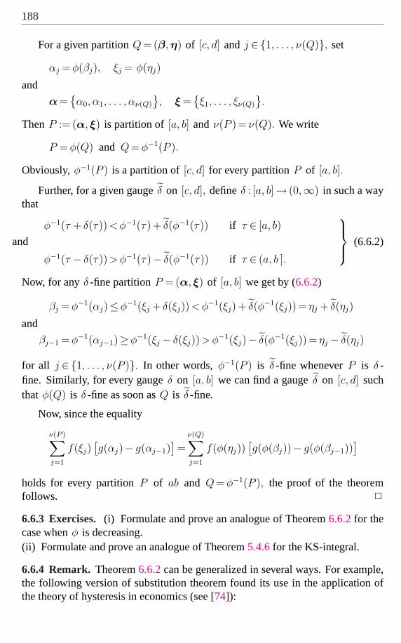
188
For a given partitionQ = (β,η) of [c, d] and j ∈{1, . . . , ν(Q)}, set
αj = φ(βj), ξj = φ(ηj)
and
α ={α0, α1, . . . , αν(Q)
}, ξ =
{ξ1, . . . , ξν(Q)
}.
ThenP := (α, ξ) is partition of [a, b] andν(P ) = ν(Q). We write
P = φ(Q) and Q = φ−1(P ).
Obviously,φ−1(P ) is a partition of[c, d] for every partitionP of [a, b].
Further, for a given gaugeδ on [c, d], defineδ : [a, b]→ (0,∞) in such a waythat
φ−1(τ + δ(τ)) <φ−1(τ) + δ(φ−1(τ)) if τ ∈ [a, b)
and
φ−1(τ − δ(τ)) >φ−1(τ)− δ(φ−1(τ)) if τ ∈ (a, b ].
(6.6.2)
Now, for anyδ -fine partitionP = (α, ξ) of [a, b] we get by (6.6.2)
βj = φ−1(αj)≤φ−1(ξj + δ(ξj)) <φ−1(ξj) + δ(φ−1(ξj)) = ηj + δ(ηj)
and
βj−1 = φ−1(αj−1)≥φ−1(ξj − δ(ξj)) >φ−1(ξj)− δ(φ−1(ξj)) = ηj − δ(ηj)
for all j ∈{1, . . . , ν(P )}. In other words,φ−1(P ) is δ -fine wheneverP is δ -fine. Similarly, for every gaugeδ on [a, b] we can find a gaugeδ on [c, d] suchthat φ(Q) is δ -fine as soon asQ is δ -fine.
Now, since the equality
ν(P )∑j=1
f(ξj)[g(αj)− g(αj−1)
]=
ν(Q)∑j=1
f(φ(ηj))[g(φ(βj))− g(φ(βj−1))
]
holds for every partitionP of ab and Q = φ−1(P ), the proof of the theoremfollows. 2
6.6.3 Exercises. (i) Formulate and prove an analogue of Theorem6.6.2for thecase whenφ is decreasing.(ii) Formulate and prove an analogue of Theorem5.4.6for the KS-integral.
6.6.4 Remark. Theorem6.6.2can be generalized in several ways. For example,the following version of substitution theorem found its use in the application ofthe theory of hysteresis in economics (see [74]):

KURZWEIL-STIELTJES INTEGRAL 189
Assume that the functionf : [a, b]→R is bounded on[a, b] and regulated on[α, b] for everyα∈ (a, b). Moreover, let the functionφ : [a, b]→R be nondecreas-ing on [a, b] and letφ(a) = c, φ(b) = d. Finally, let the functiong ∈BV([c, d]) becontinuous from the right on[c, d). Set
ψ(s) = inf{t∈ [a, b] : s≤φ(t)} fors∈ [c, d ].
Then the relation
∫ b
α
f(t) d[ g(φ(t))] =
∫ φ(b)
φ(α)
f(ψ(s)) d[ g(s)]
holds for everyα∈ [a, b].
6.7 Absolute integrability
The Kurzweil-Stieltjes integral is a nonabsolutely convergent integral – the ex-istence of
∫ b
af dg does not necessarily imply the existence of
∫ b
a|f | dg. In this
section, we collect some sufficient and necessary conditions for the existence ofthe latter integral.
We restrict our attention to the case wheng is nondecreasing. In this situation,if both
∫ b
af dg and
∫ b
a|f | dg exist, we have the inequality
∣∣∣∣∫ b
a
f dg
∣∣∣∣≤∫ b
a
|f | dg.
This fact follows immediately from the definition of the integral, since
|S(f, dg, P )| ≤S(|f |, dg, P ) for each partitionP of [a, b].
6.7.1 Theorem.Assume thatg : [a, b]→R is nondecreasing and∫ b
af dg exists.
Let
F (x) =
∫ x
a
f dg for x∈ [a, b].
Then∫ b
a|f | dg exists if and only ifF has bounded variation on[a, b]. In this
case, we have
∫ b
a
|f | dg = varbaF.

190
Proof. Suppose that∫ b
a|f | dg exists. If α is an arbitrary division of[a, b], then
V (F, α) =
ν(α)∑j=1
|F (αj)−F (αj−1)|=ν(α)∑j=1
∣∣∣∣∣∫ αj
αj−1
f dg
∣∣∣∣∣
≤ν(α)∑j=1
∫ αj
αj−1
|f | dg =
∫ b
a
|f | dg,
and therefore varbaF is finite.Conversely, suppose thatF has bounded variation on[a, b]. Consider an ar-
bitrary ε> 0 and letα be a division of[a, b] satisfying
varbaF − ε≤V (F, α)≤ varbaF.
Observe that ifβ is a refinement ofα, then
varbaF − ε≤V (F, α)≤V (F, β)≤ varbaF. (6.7.1)
Let δ be a gauge on[a, b] with the following properties:
• If P is a δ -fine partition of[a, b], then∣∣∣∫ b
af dg−S(f, dg, P )
∣∣∣ <ε.
• If i∈{1, . . . , ν(α)} and t∈ (αi−1, αi), then
(t− δ(t), t + δ(t))⊂ (αi−1, αi).
• If i∈{0, . . . , ν(α)}, then
(αi− δ(αi), αi + δ(αi))⊂ (αi−1, αi+1)
with the convention thatα−1 =−∞ andαν(α)+1 =∞.
Let P = (β, ξ) be an arbitraryδ -fine partition of [a, b]. The last two propertiesof δ ensure that each interval[βi−1, βi] is either contained in a single interval[αj−1, αj], or [βi−1, βi]⊂ [αj−1, αj+1] andξi = αj. By splitting all intervals of thesecond type in two subintervals[βi−1, ξi] and [ξi, βi] that share the same tagξi,we can obtain a new partitionP ′ such thatS(|f |, dg, P ) = S(|f |, dg, P ′). Thus,without loss of generality, we can assume thatβ is a refinement ofα.
We now use the fact thatg is nondecreasing, the reverse triangle inequality||x| − |y|| ≤ |x− y|, and finally Corollary6.5.2to obtain
∣∣∣S(|f |, dg, P )−V (F, β)∣∣∣ =
∣∣∣ν(β)∑i=1
(|f(ξi) (g(βi)− g(βi−1))| −∣∣∫ βi
βi−1
f dg∣∣)
∣∣∣
≤ν(β)∑i=1
∣∣∣f(ξi) (g(βi)− g(βi−1))−∫ βi
βi−1
f dg∣∣∣≤ 2ε.

KURZWEIL-STIELTJES INTEGRAL 191
By combining this estimate with (6.7.1), we conclude that∣∣S(|f |, dg, P )− varbaF
∣∣≤ |S(|f |, dg, P )−V (F, β)|+∣∣V (F, β)− varbaF
∣∣≤ 3ε,
which means that∫ b
a|f | dg exists and equals varb
aF. 2
6.7.2 Example.Let {tn} be an increasing sequence of points from the openinterval (0, 1) tending toτ ∈ (0, 1]. Consider the functiong : [0, 1]→R given by
g(t) =∞∑
n=1
χ[tn,1](t)1
n2. (6.7.2)
It is not hard to see thatg is nondecreasing and right-continuous on[0, 1). Letf : [0, 1]→R be defined as
f(t) =
(−1)n+1 n if t = tn for some n∈N,
0 otherwise.
Claim 1. The integral∫ 1
0f dg exists.
Note that, for eacht∈ [0, τ), the integral∫ t
0f dg exists (due to Corollary6.3.2
and using the fact that the restriction ofg to the interval[0, t] defines a finite stepfunction). Moreover, by Example6.3.1, we have
∫ t1
0
f dg = f(t1) g(t1) = 1,
and∫ tn+1
tn
f dg =
∫ tn+1
tn
f d[g(tn)χ[tn,tn+1) + g(tn+1)χ[tn+1]]
= f(tn+1) [g(tn+1)− g(tn)] =(−1)n+2
n + 1,
for eachn∈N. Since
limt→τ−
∫ t
0
f dg + f(τ)∆+g(τ) = limn→∞
∫ tn
0
f dg =∞∑
n=1
(−1)n+1
n= ln 2,
applying Hake’s Theorem (Theorem6.5.5), we conclude that the integral∫ τ
0f dg
exists and equalsln 2. If τ = 1, the claim is proved. Ifτ < 1, then∫ 1
τf dg = 0
(becauseg is constant on[τ, 1]), wherefrom the proof of the claim follows.
Claim 2. |f | is not integrable with respect tog on [0, 1].

192
Let F (t) =∫ t
0f dg for t∈ [0, 1]. We will show that var10F =∞. For every
n∈N consider the divisionDn = {0, t1, t2, . . . , tn, 1} of [0, 1]. We have
V (F, Dn) =n−1∑
k=1
∣∣∣∫ tk+1
tk
f dg∣∣∣ +
∣∣∣∫ t1
0
f dg∣∣∣ +
∣∣∣∫ 1
tn
f dg∣∣∣
=n∑
k=1
1
k+
∣∣∣∫ 1
tn
f dg∣∣∣.
SinceV (F,Dn)≤ var10F for everyn∈N, var10F cannot be finite. Thus the claimis a consequence of Theorem6.7.1.
6.7.3 Exercises.Let {tn} be an increasing sequence of points from the open in-terval (a, b) tending toτ ∈ (a, b]. Let {cn} be a sequence of nonnegative numberssuch that the series
∑cn converges. Define a functiong : [a, b]→R by
g(t) =∑
n:tn≤t
cn.
For a givenf : [a, b]→R prove that:
(i) The integral∫ b
af dg exists if and only if the series
∑cn f(tn) converges
and in such a case it is given by
∫ b
a
f dg =∞∑
n=1
cn f(tn).
(ii) The integral∫ b
a|f | dg exists if and only if the series
∑cn f(tn) is ab-
solutely convergent.
6.7.4 Theorem.Assume thatg : [a, b]→R is nondecreasing,f, h : [a, b]→R aresuch that
∫ b
af dg and
∫ b
ah dg exist and|f(t)| ≤h(t) for each t∈ [a, b]. Then∫ b
a|f | dg exists.
Proof. If [c, d]⊂ [a, b] andP is a partition of[c, d], then
|S(f, dg, P )| ≤S(h, dg, P ).
Thus, it follows from the definition of the integral that
∣∣∣∣∫ d
c
f dg
∣∣∣∣≤∫ d
c
h dg for each[c, d]⊂ [a, b].

KURZWEIL-STIELTJES INTEGRAL 193
Let
F (x) =
∫ x
a
f dg for x∈ [a, b].
If α is an arbitrary division of[a, b], we obtain the estimate
V (F, α) =
ν(α)∑i=1
|F (αi)−F (αi−1)|=ν(α)∑i=1
∣∣∣∣∫ αi
αi−1
f dg
∣∣∣∣≤ν(α)∑i=1
∫ αi
αi−1
h dg =
∫ b
a
h dg,
which shows thatF has bounded variation on[a, b]. Thus, the existence of theintegral
∫ b
a|f | dg follows from Theorem6.7.1. 2
6.7.5 Theorem.If g : [a, b]→R is nondecreasing andf1, f2 : [a, b]→R are suchthat the integrals
∫ b
af1 dg,
∫ b
af2 dg,
∫ b
a|f1| dg and
∫ b
a|f2| dg exist, then∫ b
amax(f1, f2) dg and
∫ b
amin(f1, f2) dg exist as well.
Proof. By Theorem6.7.4, the integral∫ b
a|f1− f2| dg exists, because
|f1− f2|≤|f1|+ |f2|
and the integrals∫ b
a(f1− f2) dg,
∫ b
a|f1| dg and
∫ b
a|f2| dg exist. Since
max(f1, f2) =f1 + f2 + |f1− f2|
2and min(f1, f2) =
f1 + f2− |f1− f2|2
,
the existence of∫ b
amax(f1, f2) dg and
∫ b
amin(f1, f2) dg follows from the linear-
ity of the integral (i.e., from Theorem6.1.8). 2
6.8 Convergence theorems
In this section, we present several convergence theorems for the Kurzweil-Stieltjesintegral that do not require uniform convergence.
We start by introducing the concept of uniform integrability (also known asequiintegrability).
6.8.1 Definition. Consider a sequence of functionsfn : [a, b]→R, n∈N, and afunction g : [a, b]→R. Then {fn} is called uniformly integrable with respect tog, if the following two conditions are satisfied:
• The integral∫ b
a
fn dg exists for eachn∈N.

194
• For everyε> 0, there exists a gaugeδ on [a, b] such that the inequality∣∣∣∣∫ b
a
fn dg−S(fn, dg, P )
∣∣∣∣<ε
holds for eachδ -fine partitionP of [a, b] and for everyn∈N.
The next result is a basic convergence theorem for the Kurzweil-Stieltjes inte-gral. Although the assumption of uniform integrability might be difficult to verify,the result will play a key role in deriving the other convergence theorems givenlater in this section.
6.8.2 Theorem.If {fn} is uniformly integrable with respect tog and
limn→∞
fn(t) = f(t) for all t∈ [a, b],
then both the integral∫ b
af dg and the limitlimn→∞
∫ b
afn dg exist, and the equal-
ity∫ b
a
f dg = limn→∞
∫ b
a
fn dg
is true.
Moreover,
limn→∞
(sup
t∈[a,b]
∣∣∣∣∫ t
a
fn dg−∫ t
a
f dg
∣∣∣∣)
= 0 (6.8.1)
holds wheneverg is bounded on[a, b].
Proof. a) Consider an arbitraryε> 0 and letδ be the corresponding gauge fromDefinition6.8.1. Choose an arbitraryδ -fine partitionP of [a, b]. Since
limn→∞
S(fn, dg, P ) = S(f, dg, P ),
there exists ann0 ∈N such that
|S(fm, dg, P )−S(fn, dg, P )|<ε
holds for all m,n≥n0. Using this fact together with the definition of uniformintegrability, we get
∣∣∣∣∫ b
a
fm dg−∫ b
a
fn dg
∣∣∣∣
≤∣∣∣∣∫ b
a
fm dg−S(fm, dg, P )
∣∣∣∣ + |S(fm, dg, P )−S(fn, dg, P )|
+
∣∣∣∣S(fn, dg, P )−∫ b
a
fn dg
∣∣∣∣< 3 ε

KURZWEIL-STIELTJES INTEGRAL 195
for all m,n≥n0. In particular,{∫ b
afn dg} is a Cauchy sequence and thus it has
a finite limit:
limn→∞
∫ b
a
fn dg = L∈R.
Now, let P be an arbitraryδ -fine partition of[a, b]. Choose ann1 ∈N such that
|S(fn1 , dg, P )−S(f, dg, P )|<ε and
∣∣∣∣∫ b
a
fn1 dg−L
∣∣∣∣ <ε.
Then
|S(f, dg, P )−L| ≤ |S(f, dg, P )−S(fn1 , dg, P )|
+
∣∣∣∣S(fn1 , dg, P )−∫ b
a
fn1 dg
∣∣∣∣ +
∣∣∣∣∫ b
a
fn1 dg−L
∣∣∣∣ < 3ε.
It follows that∫ b
af dg exists and equalsL.
b) To prove (6.8.1), let hn(t) = fn(t)− f(t) for n∈N and t∈ [a, b], and assumethat g is bounded on[a, b]. Note that the sequence{hn} tends pointwise on[a, b]to 0 and it is uniformly integrable with respect tog. Choose an arbitraryε> 0and find a gaugeδ on [a, b] such that
∣∣∣∣∫ b
a
hn dg−S(hn, dg, P )
∣∣∣∣<ε (6.8.2)
for eachδ -fine partitionP of [a, b]. Let P = (α, ξ) be such a partition. Sincehn(t)→ 0 for t∈ [a, b] andg is bounded, there exists ann0 ∈N such that
|hn(ξi)| ‖g‖<ε
2 ν(α)for all n≥n0 andi∈{1, . . . , ν(α)}. (6.8.3)
Let arbitraryt∈ [a, b] andn∈N∩ [n0,∞) be given and letj ∈{1, . . . , ν(α)} besuch thatt∈ [αj−1, αj]. Then,
∣∣∣∣∫ t
a
hn dg
∣∣∣∣ =
∣∣∣∣∣j−1∑i=1
∫ αi
αi−1
hn dg +
∫ t
αj−1
hn dg
∣∣∣∣∣
≤∣∣∣
j−1∑i=1
(∫ αi
αi−1
hn dg−hn(ξi) (g(αi)− g(αi−1))
)
+
∫ t
αj−1
hn dg−hn(ξj) (g(t)− g(αj−1))∣∣∣
+
j−1∑i=1
|hn(ξi)| |g(αi)− g(αi−1)|+ |hn(ξj)| |g(t)− g(αj−1)|.

196
Due to (6.8.3) we have
j−1∑i=1
|hn(ξi)| |g(αi)− g(αi−1)|+ |hn(ξj)| |g(t)− g(αj−1)|
≤j∑
i=1
2 |hn(ξi)| ‖g‖<ε.
Furthermore, ift≥ ξj, then, having in mind (6.8.2), we may apply the Saks-Henstock lemma to the system
{([αi−1, αi], ξi) : i = 1, . . . , j− 1}∪ {([αj−1, t], ξj)}
and deduce that∣∣∣∣∣
j−1∑i=1
(∫ αi
αi−1
hn dg−hn(ξi) (g(αi)− g(αi−1))
)
+
∫ t
αj−1
hn dg−hn(ξj) (g(t)− g(αj−1))
∣∣∣∣∣≤ ε.
On the other hand, ift< ξj, then applying the Saks-Henstock lemma to the sys-tems
{([αi−1, αi], ξi) : i = 1, . . . , j}} and
{([t, αj], ξj)
},
we get
∣∣∣∣∣j−1∑i=1
(∫ αi
αi−1
hn dg−hn(ξi) (g(αi)− g(αi−1))
)
+
∫ t
αj−1
hn dg−hn(ξj) (g(t)− g(αj−1))
∣∣∣∣∣
=
∣∣∣∣∣j∑
i=1
(∫ αi
αi−1
hn dg−hn(ξi) (g(αi)− g(αi−1))
)
−(∫ αj
t
hn dg−hn(ξj) (g(αj)− g(t))
) ∣∣∣∣∣≤ 2 ε.
To summarize, we have shown that∣∣∣∣∫ t
a
hn dg
∣∣∣∣≤ 3 ε for all n≥n0 and t∈ [a, b],

KURZWEIL-STIELTJES INTEGRAL 197
which completes the proof of (6.8.1). 2
The next example shows that the boundedness of the integratorg is essentialto ensure the uniform convergence of the indefinite integrals in (6.8.1).
6.8.3 Example.Let fn(t) = 1/n for t∈ [a, b] and letg : [a, b]→R be arbitrarywith g(a) = 0. Then {fn} tends pointwise on[a, b] to the zero function. Fur-thermore, asS(fn, dg, P ) = (1/n) g(b) for eachn∈N and each partitionP of[a, b], we see that
∫ b
afn dg = (1/n) g(b) for eachn∈N and the sequence{fn}
is uniformly integrable with respect tog. However, we claim that the indefiniteintegralsFn(t) =
∫ t
afn dg tend uniformly to the zero function if and only ifg
is bounded. Indeed, we haveFn(t) = (1/n) g(t) for t∈ [a, b]. Clearly, if g isbounded on[a, b], then {Fn} tends uniformly on[a, b] to the zero function. Onthe other hand, ifg is unbounded and an arbitraryε> 0 is given, then for eachn∈N, there is at∈ [a, b] such that
|Fn(t)|= |(1/n) g(t)|>ε,
i.e., Fn does not converge uniformly to the zero function.
The remaining convergence theorems in this section provide more transparentconditions that imply uniform integrability. To proceed, we need the followingauxiliary lemma.
6.8.4 Lemma.For each`∈N, let S` be the set of all couples(σ, s), whereσ isa division of[a, b] and s = {s1, . . . , sν(σ)} is a finite sequence of integers greaterthan or equal to .
Let g : [a, b]→R and let fn : [a, b]→R, n∈N, be a sequence of functionssuch that the integral
∫ b
afn dg exists for eachn∈N. Moreover, assume that there
are B, C ∈R such that ifσ is a division of[a, b] and s1, . . . , sν(σ) ∈N, then
B≤ν(σ)∑j=1
∫ σj
σj−1
fsjdg≤C. (6.8.4)
Then for eachε> 0 and `∈N there exist(π`, p`), (ρ`, r`)∈S` such that thefollowing statements are true:
(i) The inequalities
ν(π`)∑j=1
∫ π`j
π`j−1
fp`j
dg− ε
2`<
ν(σ)∑j=1
∫ σj
σj−1
fsjdg <
ν(ρ`)∑j=1
∫ ρ`j
ρ`j−1
fr`j
dg +ε
2`(6.8.5)
hold for each(σ, s)∈S`.

198
(ii) Assume thatI =⋃
i∈I [ci, di] is a finite union of nonoverlapping intervalsin [a, b] such that for eachi∈ I there is aj(i)∈{1, . . . , ν(π`)} satisfying[ci, di]⊂ [π`
j(i)−1, π`j(i)]. Then the inequality
∑i∈I
∫ di
ci
fp`j(i)
dg− ε
2`<
∑i∈I
∫ di
ci
fn dg (6.8.6)
holds for eachn≥ `.
(iii) Assume thatI =⋃
i∈I [ci, di] is a finite union of nonoverlapping intervalsin [a, b] such that for eachi∈ I there exists aj(i)∈{1, . . . , ν(ρ`)} satis-fying [ci, di]⊂ [ρ`
j(i)−1, ρ`j(i)]. Then the inequality
∑i∈I
∫ di
ci
fn dg <∑i∈I
∫ di
ci
fr`j(i)
dg +ε
2`(6.8.7)
holds for eachn≥ `.
Proof. According to (6.8.4), the values of all sums
ν(σ)∑j=1
∫ σj
σj−1
fsjdg, where (σ, s)∈S`,
are contained in a bounded subset ofR. Thus, the existence of the couples(π`,p`)and (ρ`, r`)∈S` having the properties from statement (i) follows from the defin-itions of infimum and supremum.
To prove statement (ii), consider the divisionσ = π` ∪{ci, di : i∈ I} of [a, b].For each j ∈{1, . . . , ν(σ)}, there exists ak(j)∈{1, . . . , ν(π`)} such that[σj−1, σj]⊂ [π`
k(j)−1, π`k(j)]. Defines as follows: If j ∈{1, . . . , ν(σ)} is such that
[σj−1, σj]⊂I, let sj = n. Otherwise, letsj = p`k(j). Then (σ, s)∈S`, and rela-
tion (6.8.5) holds. Obviously,
ν(σ)∑j=1
∫ σj
σj−1
fsjdg =
∑
j∈{1,...,ν(σ)}[σj−1,σj ]⊂I
∫ σj
σj−1
fn dg +∑
j∈{1,...,ν(σ)}[σj−1,σj ]6⊂I
∫ σj
σj−1
fp`k(j)
dg
=∑i∈I
∫ di
ci
fn dg +∑
j∈{1,...,ν(σ)}[σj−1,σj ]6⊂I
∫ σj
σj−1
fp`k(j)
dg
Furthermore, for eachm∈{1, . . . , ν(π`)}, we have
[π`m−1, π
`m] =
⋃
j∈{1,...,ν(σ)}k(j)=m
[σj−1, σj],

KURZWEIL-STIELTJES INTEGRAL 199
and therefore
ν(π`)∑j=1
∫ π`j
π`j−1
fp`j
dg =
ν(π`)∑m=1
∑
j∈{1,...,ν(σ)}k(j)=m
∫ σj
σj−1
fp`m
dg =
ν(σ)∑j=1
∫ σj
σj−1
fp`k(j)
dg
=∑
j∈{1,...,ν(σ)}[σj−1,σj ]⊂I
∫ σj
σj−1
fp`k(j)
dg +∑
j∈{1,...,ν(σ)}[σj−1,σj ]6⊂I
∫ σj
σj−1
fp`k(j)
dg
=∑i∈I
∫ di
ci
fp`j(i)
dg +∑
j∈{1,...,ν(σ)}[σj−1,σj ]6⊂I
∫ σj
σj−1
fp`k(j)
dg.
Now, by subtracting
∑
j∈{1,...,ν(σ)}[σj−1,σj ]6⊂I
∫ σj
σj−1
fp`k(j)
dg
from the first inequality in (6.8.5), we get (6.8.6).
Statement (iii) can be proved in a similar way. 2
The following convergence theorem is due to D. Preiss andS. Schwabik. It isa special case of Theorem 5.5 from J. Kurzweil’s book [81], which is concernedwith a more general type of integral; see also Theorem 1.28 and Remark 1.30 in[122].
6.8.5 Theorem.Let g ∈BV([a, b]) and let {fn} be a sequence of real valuedfunctions defined on[a, b] and satisfying the following conditions:
(i) The integral∫ b
afn dg exists for eachn∈N.
(ii) limn→∞
fn(t) = f(t) for t∈ [a, b].
(iii) There areB, C ∈R such that the inequalities
B≤ν(σ)∑j=1
∫ σj
σj−1
fsjdg≤C
hold for all divisionsσ of [a, b] and all s1, . . . , sν(σ) ∈N.
Then{fn} is uniformly integrable with respect tog, the integral∫ b
af dg exists,
and∫ b
a
f dg = limn→∞
∫ b
a
fn dg.
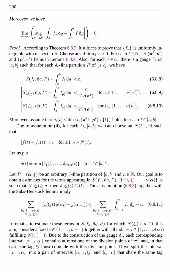
200
Moreover, we have
limn→∞
(sup
t∈[a,b]
∣∣∣∣∫ t
a
fn dg−∫ t
a
f dg
∣∣∣∣)
= 0.
Proof. According to Theorem6.8.2, it suffices to prove that{fn} is uniformly in-tegrable with respect tog. Choose an arbitraryε> 0. For each ∈N, let (π`,p`)and (ρ`, r`) be as in Lemma6.8.4. Also, for each`∈N, there is a gaugeδ` on[a, b] such that for eachδ` -fine partitionP of [a, b], we have
∣∣∣∣S(f`, dg, P )−∫ b
a
f` dg
∣∣∣∣ <ε, (6.8.8)∣∣∣∣S(fp`
i, dg, P )−
∫ b
a
fp`i
dg
∣∣∣∣ <ε
2`ν(π`)for i∈{1, . . . , ν(π`)}, (6.8.9)
∣∣∣∣S(fr`i, dg, P )−
∫ b
a
fr`i
dg
∣∣∣∣ <ε
2`ν(ρ`)for i∈{1, . . . , ν(ρ`)}. (6.8.10)
Moreover, assume thatδ`(t) < dist(t, (π` ∪ρ`) \ {t}) holds for eacht∈ [a, b].
Due to assumption (ii), for eacht∈ [a, b] we can choose anN(t)∈N suchthat
|f(t)− fn(t)|<ε for all n≥N(t).
Let us put
δ(t) = min{δ1(t), . . . , δN(t)(t)} for t∈ [a, b].
Let P = (α, ξ) be an arbitraryδ -fine partition of[a, b] andn∈N. Our goal is toobtain estimates for the terms appearing inS(fn, dg, P ). If i∈{1, . . . , ν(α)} issuch thatN(ξi)≥n, then δ(ξi)≤ δn(ξi). Thus, assumption (6.8.8) together withthe Saks-Henstock lemma imply
∑
i∈{1,...,ν(α)}N(ξi)≥n
fn(ξi) (g(αi)− g(αi−1))≤∑
i∈{1,...,ν(α)}N(ξi)≥n
∫ αi
αi−1
fn dg + ε. (6.8.11)
It remains to estimate those terms inS(fn, dg, P ) for which N(ξi) <n. To thisaim, consider a fixed∈{1, . . . , n− 1} together with all indicesi∈{1, . . . , ν(α)}fulfilling N(ξi) = `. Due to the construction of the gaugeδ`, each correspondinginterval [αi−1, αi] contains at most one of the division points ofπ` and, in thatcase, the tagξi must coincide with this division point. If we split the interval[αi−1, αi] into a pair of intervals[αi−1, ξi] and [ξi, αi] that share the same tag
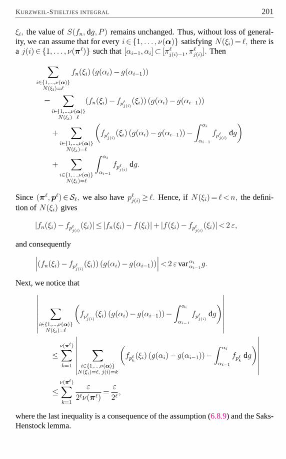
KURZWEIL-STIELTJES INTEGRAL 201
ξi, the value ofS(fn, dg, P ) remains unchanged. Thus, without loss of general-ity, we can assume that for everyi∈{1, . . . , ν(α)} satisfyingN(ξi) = `, there isa j(i)∈{1, . . . , ν(π`)} such that[αi−1, αi]⊂ [π`
j(i)−1, π`j(i)]. Then
∑
i∈{1,...,ν(α)}N(ξi)=`
fn(ξi) (g(αi)− g(αi−1))
=∑
i∈{1,...,ν(α)}N(ξi)=`
(fn(ξi)− fp`j(i)
(ξi)) (g(αi)− g(αi−1))
+∑
i∈{1,...,ν(α)}N(ξi)=`
(fp`
j(i)(ξi) (g(αi)− g(αi−1))−
∫ αi
αi−1
fp`j(i)
dg
)
+∑
i∈{1,...,ν(α)}N(ξi)=`
∫ αi
αi−1
fp`j(i)
dg.
Since (π`,p`)∈S`, we also havep`j(i)≥ `. Hence, if N(ξi) = `< n, the defini-
tion of N(ξi) gives
|fn(ξi)− fp`j(i)
(ξi)| ≤ |fn(ξi)− f(ξi)|+ |f(ξi)− fp`j(i)
(ξi)|< 2 ε,
and consequently∣∣∣(fn(ξi)− fp`
j(i)(ξi)) (g(αi)− g(αi−1))
∣∣∣< 2 ε varαiαi−1
g.
Next, we notice that∣∣∣∣∣∣∣∣
∑
i∈{1,...,ν(α)}N(ξi)=`
(fp`
j(i)(ξi) (g(αi)− g(αi−1))−
∫ αi
αi−1
fp`j(i)
dg
)∣∣∣∣∣∣∣∣
≤ν(π`)∑
k=1
∣∣∣∣∣∣∣∣
∑
i∈{1,...,ν(α)}N(ξi)=`, j(i)=k
(fp`
k(ξi) (g(αi)− g(αi−1))−
∫ αi
αi−1
fp`k
dg
)∣∣∣∣∣∣∣∣
≤ν(π`)∑
k=1
ε
2`ν(π`)=
ε
2`,
where the last inequality is a consequence of the assumption (6.8.9) and the Saks-Henstock lemma.

202
To summarize, for each∈{1, . . . , n− 1} the previous estimates imply∑
i∈{1,...,ν(α)}N(ξi)=`
fn(ξi) (g(αi)− g(αi−1))
<∑
i∈{1,...,ν(α)}N(ξi)=`
(∫ αi
αi−1
fp`j(i)
dg + 2 ε varαiαi−1
g
)+
ε
2`
<∑
i∈{1,...,ν(α)}N(ξi)=`
(∫ αi
αi−1
fn dg + 2 ε varαiαi−1
g
)+ 2
ε
2`,
where the last inequality follows from (6.8.6). Summation over ∈{1, . . . , n− 1}yields
∑
i∈{1,...,ν(α)}N(ξi)<n
fn(ξi) (g(αi)− g(αi−1)) <∑
i∈{1,...,ν(α)}N(ξi)<n
∫ αi
αi−1
fn dg + 2 ε varbag + 2 ε.
Adding the last inequality and (6.8.11), we conclude that the estimate
S(fn, dg, P ) =
ν(α)∑i=1
fn(ξi) (g(αi)− g(αi−1)) <
∫ b
a
fn dg + 2 ε varbag + 3 ε
holds for all n∈N. Proceeding in a similar way (using (6.8.7) and (6.8.10)), wecan show that also
S(fn, dg, P ) >
∫ b
a
fn dg− 2 ε varbag− 3 ε
holds for alln∈N. As a consequence,∣∣∣∣S(fn, dg, P )−
∫ b
a
fn dg
∣∣∣∣< 2 ε varbag + 3 ε
for eachδ -fine partitionP of [a, b] and eachn∈N, i.e., {fn} is uniformly inte-grable with respect tog. 2
A straightforward consequence of Theorem6.8.5 is the dominated conver-gence theorem.
6.8.6 Theorem(DOMINATED CONVERGENCE THEOREM).Let g : [a, b]→R be nondecreasing and let{fn} be a sequence of real valuedfunctions defined on[a, b] and satisfying the following conditions:

KURZWEIL-STIELTJES INTEGRAL 203
• The integral∫ b
afn dg exists for eachn∈N.
• limn→∞
fn(t) = f(t) for t∈ [a, b].
• There exist functionsh1, h2 : [a, b]→R such that the integrals∫ b
ah1 dg,∫ b
ah2 dg exist andh1≤ fn≤h2 on [a, b] for eachn∈N.
Then{fn} is uniformly integrable with respect tog, the integral∫ b
af dg exists
and
∫ b
a
f dg = limn→∞
∫ b
a
fn dg.
Moreover, we have
limn→∞
(sup
t∈[a,b]
∣∣∣∣∫ t
a
fn dg−∫ t
a
f dg
∣∣∣∣)
= 0.
Proof. The statement is a consequence of Theorem6.8.5. To see this, let
B =
∫ b
a
h1 dg, C =
∫ b
a
h2 dg.
If σ is a division of[a, b] ands1, . . . , sν(σ) ∈N, then
B =
ν(σ)∑j=1
∫ σj
σj−1
h1 dg≤ν(σ)∑j=1
∫ σj
σj−1
fsjdg≤
ν(σ)∑j=1
∫ σj
σj−1
h2 dg = C.
This shows that the assumptions of Theorem6.8.5are satisfied, and the proof iscomplete. 2
6.8.7 Remark. In the previous theorem, the conditionh1≤ fn≤h2 on [a, b] canbe weakened. It is enough to assume that for each interval[c, d]⊂ [a, b] and eachn∈N, we have
∫ d
c
h1 dg≤∫ d
c
fn dg≤∫ d
c
h2 dg.
In a similar way, we can derive the bounded convergence theorem. In com-parison with the dominated convergence theorem, the dominating hypothesis on{fn} is stronger. On the other hand,g is no longer assumed to be nondecreasing,but merely of bounded variation.

204
6.8.8 Theorem(BOUNDED CONVERGENCE THEOREM).Let g ∈BV([a, b]) and let{fn} be a sequence of real valued functions defined on[a, b] and satisfying the following conditions:
• The integral∫ b
afn dg exists for eachn∈N.
• limn→∞
fn = f on [a, b].
• There exists a constantM ≥ 0 such that |fn(t)| ≤M for all n∈N andt∈ [a, b].
Then{fn} is uniformly integrable with respect tog, the integral∫ b
af dg exists
and
limn→∞
(sup
t∈[a,b]
∣∣∣∣∫ t
a
fn dg−∫ t
a
f dg
∣∣∣∣)
= 0.
Proof. If σ is a division of[a, b] ands1, . . . , sν(σ) ∈N, then
∣∣∣∣∣∣
ν(σ)∑j=1
∫ σj
σj−1
fsjdg
∣∣∣∣∣∣≤
ν(σ)∑j=1
∣∣∣∣∣∫ σj
σj−1
fsjdg
∣∣∣∣∣≤ν(σ)∑j=1
M varσjσj−1
g = M varbag.
Hence, the assumptions of Theorem6.8.5are satisfied with
B =−M varbag, C = M varbag,
and the proof is complete. 2
Another important consequence of Theorem6.8.5 is the monotone conver-gence theorem.
6.8.9 Theorem(MONOTONE CONVERGENCE THEOREM).Let g : [a, b]→R be nondecreasing and{fn} be a sequence of functions such thatthe integral
∫ b
afn dg exists for eachn∈N, and lim
n→∞fn = f on [a, b]. Suppose,
in addition, that one of the following conditions holds:
• {fn} is a nondecreasing sequence andlimn→∞
∫ b
a
fn dg <∞.
• {fn} is a nonincreasing sequence andlimn→∞
∫ b
a
fn dg >−∞.

KURZWEIL-STIELTJES INTEGRAL 205
Then{fn} is uniformly integrable with respect tog, the integral∫ b
af dg exists
and∫ b
a
f dg = limn→∞
∫ b
a
fn dg. (6.8.12)
Moreover, we have
limn→∞
(sup
t∈[a,b]
∣∣∣∣∫ t
a
fn dg−∫ t
a
f dg
∣∣∣∣)
= 0. (6.8.13)
Proof. Suppose that the first condition holds. Let
B =
∫ b
a
f1 dg, C = limn→∞
∫ b
a
fn dg.
If σ is a division of[a, b] ands1, . . . , sν(σ) ∈N, then
B =
ν(σ)∑j=1
∫ σj
σj−1
f1 dg≤ν(σ)∑j=1
∫ σj
σj−1
fsjdg≤
ν(σ)∑j=1
∫ σj
σj−1
(fmax(s1,...,sν(σ))) dg≤C.
Thus, the assumptions of Theorem6.8.5are satisfied, and (6.8.12), (6.8.13) hold.If the second condition holds, it is enough to consider the sequence{−fn}, whichobviously satisfies the first condition. 2
The monotone convergence theorem has a number of useful corollaries, whichwill be needed later. The first result is an analogue of Levi’s theorem for term-by-term integration of infinite series.
6.8.10 Theorem.Suppose thatg : [a, b]→R is nondecreasing,fk : [a, b]→R isa nonnegative function for eachk ∈N, and f =
∑∞k=1 fk on [a, b]. If the integral∫ b
afk dg exists for eachk ∈N and if the sum
∑∞k=1
∫ b
afk dg is finite, then the se-
quence{sn} given bysn =∑n
k=1 fk on [a, b] is uniformly integrable with respectto g and
∫ b
a
f dg =∞∑
k=1
∫ b
a
fk dg.
Moreover, we have
limn→∞
(sup
t∈[a,b]
∣∣∣∣∫ t
a
sn dg−∫ t
a
f dg
∣∣∣∣)
= 0.
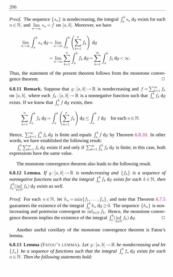
206
Proof. The sequence{sn} is nondecreasing, the integral∫ b
asn dg exists for each
n∈N, and limn→∞
sn = f on [a, b]. Moreover, we have
limn→∞
∫ b
a
sn dg = limn→∞
∫ b
a
(n∑
k=1
fk
)dg
= limn→∞
n∑
k=1
∫ b
a
fk dg =∞∑
k=1
∫ b
a
fk dg <∞.
Thus, the statement of the present theorem follows from the monotone conver-gence theorem. 2
6.8.11 Remark. Suppose thatg : [a, b]→R is nondecreasing andf =∑∞
k=1 fk
on [a, b], where eachfk : [a, b]→R is a nonnegative function such that∫ b
afk dg
exists. If we know that∫ b
af dg exists, then
n∑
k=1
∫ b
a
fk dg =
∫ b
a
(n∑
k=1
fk
)dg≤
∫ b
a
f dg for eachn∈N.
Hence,∑∞
k=1
∫ b
afk dg is finite and equals
∫ b
af dg by Theorem6.8.10. In other
words, we have established the following result:∫ b
a
∑∞k=1 fk dg exists if and only if
∑∞k=1
∫ b
afk dg is finite; in this case, both
expressions have the same value.
The monotone convergence theorem also leads to the following result.
6.8.12 Lemma. If g : [a, b]→R is nondecreasing and{fk} is a sequence ofnonnegative functions such that the integral
∫ b
afk dg exists for eachk ∈N, then∫ b
a(infk∈N
fk) dg exists as well.
Proof. For eachn∈N, let hn = min{f1, . . . , fn}, and note that Theorem6.7.5guarantees the existence of the integral
∫ b
ahn dg≥ 0. The sequence{hn} is non-
increasing and pointwise convergent toinfk∈N fk. Hence, the monotone conver-gence theorem implies the existence of the integral
∫ b
a(infk∈N
fk) dg. 2
Another useful corollary of the monotone convergence theorem is Fatou’slemma.
6.8.13 Lemma(FATOU’ S LEMMA). Let g : [a, b]→R be nondecreasing and let{fn} be a sequence of functions such that the integral
∫ b
afn dg exists for each
n∈N. Then the following statements hold:

KURZWEIL-STIELTJES INTEGRAL 207
(i) Assume there is a functionϕ : [a, b]→R such that∫ b
aϕ dg exists and
fn≥ϕ on [a, b] for eachn∈N. If lim infn→∞
fn(x) <∞ for eachx∈ [a, b]
and lim infn→∞
∫ b
afn dg <∞, then
∫ b
a(lim inf
n→∞fn) dg exists, and we have
∫ b
a
(lim infn→∞
fn) dg≤ lim infn→∞
∫ b
a
fn dg.
(ii) Assume there is a functionψ : [a, b]→R such that∫ b
aψ dg exists and
fn≤ψ for each n∈N. If lim supn→∞
fn(x) >−∞ for each x∈ [a, b] and
lim supn→∞
∫ b
afn dg >−∞, then
∫ b
a(lim sup
n→∞fn) dg exists, and we have
∫ b
a
(lim supn→∞
fn) dg≥ lim supn→∞
∫ b
a
fn dg.
Proof. Let us prove the first statement. Without loss of generality, we can assumethat ϕ = 0 (otherwise, it is enough to consider the sequence{fn−ϕ}). For eachn∈N, let hn = inf
k≥nfk. The sequence{hn} consists of nonnegative functions, it
is nondecreasing, and pointwise convergent tolim infn→∞
fn. By Lemma6.8.12, the
integral∫ b
ahn dg exists for eachn∈N. Obviously, we have
∫ b
a
hn dg≤∫ b
a
fn dg,
and therefore
limn→∞
∫ b
a
hn dg = lim infn→∞
∫ b
a
hn dg≤ lim infn→∞
∫ b
a
fn dg <∞.
The monotone convergence theorem implies the existence of the integral∫ b
a( limn→∞
hn) dg, and we get
∫ b
a
(lim infn→∞
fn) dg =
∫ b
a
( limn→∞
hn) dg = limn→∞
∫ b
a
hn dg≤ lim infn→∞
∫ b
a
fn dg.
To prove that the second statement holds, it is enough to consider the sequence{−fn} and apply the first statement. 2
6.9 Integration over elementary sets
Up to now we have been discussing the integration over a fixed given interval,more precisely, integration from some lower bound to some upper bound. In the

208
theory of the Lebesgue integral one can meet also the possibility of integrationover more general sets. The generality of the Kurzweil-Stieltjes integral (in thesense of a large domain of integrable functions) seems to be the source of troubleswith defining the Kurzweil-Stieltjes integral over general sets, in particular in thecases when we do not want to restrict ourselves to continuous integrators. Areasonable compromise seems to be to restrict the considerations to elementarysets (cf. Definition2.8.10). In this case the following definition turned out to beuseful for our purposes.
6.9.1 Definition. Let f : [a, b]→R, g : [a, b]→R and an elementary subsetE of[a, b] be given. The Kurzweil-Stieltjes integral off with respect tog over E isgiven by
∫
E
f dg =
∫ b
a
(f χE) dg
provided the integral on the right-hand side exists.
According to Definition6.9.1, the existence of the integral∫
Ef dg means
that there is anI ∈R such that for everyε> 0 there is a gaugeδ on [a, b] suchthat
∣∣S(fχE, dg, P )− I∣∣<ε for all δ-fine partitionsP on [a, b].
As we will see later, the value of the integral∫
Ef dg can depend on the choice
of the interval[a, b] which containsE . Hence, throughout this section the interval[a, b] is assumed to be fixed. Further, we use extensively the following conventionmentioned in the point (x) of Conventions and notation: Functionsg defined onthe interval[a, b] are supposed to be extended to some open interval containing[a, b] in such a way that
g(a−) = g(a), g(b+) = g(b), i.e. ∆−g(a) = ∆+g(b) = 0.
The basic properties of the Kurzweil-Stieltjes integral over elementary setsgiven below are immediate consequences of the corresponding properties of theKurzweil-Stieltjes integral presented in the previous sections.
6.9.2 Theorem.Let E be an elementary subset of[a, b]. Assume that the func-tions f, f1, f2, g, g1, g2 : [a, b]→R are such that the integrals
∫
E
f1 dg,
∫
E
f2 dg,
∫
E
f dg1 and∫
E
f dg2
exist. Then for anyc1, c2 ∈R,∫
E
(c1f1 + c2f2) dg = c1
∫
E
f1 dg + c2
∫
E
f2 dg
and

KURZWEIL-STIELTJES INTEGRAL 209
∫
E
f d[c1 g1 + c2 g2] = c1
∫
E
f d[g1] + c2
∫
E
f d[g2]
hold.
Using Theorem6.9.2the following additivity result of the integral with respectto elementary sets can be justified.
6.9.3 Theorem.Let E1 and E2 be disjoint elementary subsets of[a, b] . Assumethat f, g : [a, b]→R are such that both the integrals
∫
E1
f dg and∫
E2
f dg
exist. Then the integral∫
E1∪E2f dg exists as well and
∫
E1∪E2
f dg =
∫
E1
f dg +
∫
E2
f dg.
6.9.4 Remark. Note that if E is an elementary subset of[a, b] and h = 0 onE, then obviously
∫E
h dg = 0 for eachg : [a, b]→R. Therefore, if the integral∫E
f1 dg exists, then the equality∫
E
f1 dg =
∫
E
f2 dg
holds for each functionf2 such thatf2 = f1 on E.
Later in this section we will provide conditions ensuring the existence of theintegral over elementary sets (see Corollary6.9.10). For now, let us simply high-light the following result which is a consequence of Theorem6.3.8.
6.9.5 Theorem.Let f ∈G([a, b]) and g ∈BV([a, b]). If E is an elementary sub-set of[a, b], then the integral
∫E
f dg exists.
Proof. It is enough to observe thatf χE : [a, b]→R is a regulated function when-everf ∈G([a, b]) andE is an elementary subset of[a, b]. 2
Now we are going to consider the properties of integrals over arbitrary boun-ded intervals. For degenerate intervals, i.e., singleton sets, we have the followingresult.
6.9.6 Theorem.Let τ ∈ [a, b] and let g : [a, b]→R have finite one-sided limitsg(τ−) and g(τ+) . Then the integral
∫[τ ]
f dg exists and
∫
[τ ]
f dg = f(τ) ∆g(τ). (6.9.1)

210
Proof. Note that(fχ[τ ]
)(t) = f(τ)χ[τ ](t) for all t∈ [a, b] . Hence,
∫
[τ ]
f dg =
∫ b
a
fχ[τ ] dg = f(τ)
∫ b
a
χ[τ ] dg
and the result follows from Example6.3.1(iii). 2
Integration over subintervals of[a, b] is described by the following assertion.
6.9.7 Theorem.Let f : [a, b]→R, g ∈G([a, b]) and a≤ c< d≤ b. Then if oneof the integrals
∫
[c,d]
f dg,
∫
(c,d)
f dg,
∫
[c,d)
f dg,
∫
(c,d]
f dg,
∫ d
c
f dg (6.9.2)
exists, all the others exist as well. In this case, we have the following equalities:
∫
[c,d]
f dg = f(c) ∆−g(c) +
∫ d
c
f dg + f(d) ∆+g(d), (6.9.3)
∫
(c,d)
f dg =−f(c) ∆+g(c) +
∫ d
c
f dg− f(d) ∆−g(d), (6.9.4)
∫
[c,d)
f dg = f(c) ∆−g(c) +
∫ d
c
f dg− f(d) ∆−g(d), (6.9.5)
∫
(c,d]
f dg =−f(c) ∆+g(c) +
∫ d
c
f dg + f(d) ∆+g(d). (6.9.6)
Proof. Note that
∫
[c,d]
f dg =
∫ c
a
(fχ[c,d]) dg +
∫ d
c
f dg +
∫ b
d
(fχ[c,d]) dg.
Clearly, the first and third integral on the right-hand side exist by Examples 6.3.1(iii). Thus, the integral over[c, d] exists if and only if the integral
∫ d
cf dg exists.
In this case,
∫
[c,d]
f dg = f(c)
∫ c
a
χ[c] dg +
∫ d
c
f dg + f(d)
∫ b
d
χ[d] dg
= f(c) ∆−g(c) +
∫ d
c
f dg + f(d) ∆+g(d).
Since by Theorem6.9.6, both integrals∫
[c]f dg and
∫[d]
f dg exist, the equiva-lence between the existence of the integral over[c, d] and the existence of integral

KURZWEIL-STIELTJES INTEGRAL 211
over the open or half-open corresponding intervals can be easily derived from therelations
χ[c,d] = χ[c] + χ(c,d) + χ[d] = χ[c] + χ(c,d] = χ[c,d) + χ[d].
The equalities (6.9.4), (6.9.5) and (6.9.6) follow from (6.9.3) using Theorem6.9.6.The detailed proof is left as an exercise for the reader. 2
6.9.8 Remark. According to Theorem6.9.7, given f : [a, b]→R, g ∈C([a, b])and a≤ c≤ d≤ b , such that one of the integrals in (6.9.2) exists, then
∫
[c,d)
f dg =
∫
(c,d]
f dg =
∫
(c,d)
f dg =
∫ d
c
f dg =
∫
[c,d]
f dg.
We are now ready to evaluate integrals over elementary sets. To this end, wewill make use of the notion of minimal decomposition of an elementary set (seeDefinition2.8.9).
6.9.9 Theorem.Let f : [a, b]→R, g ∈G([a, b]) and letE be an elementary sub-set of [a, b] with the minimal decomposition{Jk : k = 1, . . . , N}. If the integral∫
Ef dg exists, then also the integrals
∫Jk
f dg exist for all k ∈{1, . . . , N} and
∫
E
f dg =N∑
k=1
∫
Jk
f dg. (6.9.7)
Proof. For k = 1, . . . , N, let ck = inf Jk anddk = sup Jk . By the hypothesis, theintegral
∫
E
f dg =
∫ b
a
(fχE) dg
exists, and hence, by Theorem6.1.10, so do all the integrals
∫ dk
ck
(fχE) dg for k ∈{1, . . . , N}.
Note that∫ dk
ck
f(χE −χJk) dg = 0, for k ∈{1, . . . , N}
(due to the fact thatf(χE −χJk) vanishes on[ck, dk]) and, similarly, the integrals
∫ ck
a
(fχJk) dg and
∫ b
dk
(fχJk) dg

212
are either zero or integrals over singleton sets (depending on whetherck and/ordk belong toJk ). Since all of these integrals exist, we conclude that
∫
Jk
f dg =
∫ b
a
(f χJk) dg
exist for all k ∈{1, . . . , N}. Having in mind that the intervals of the minimaldecomposition are pairwise disjoint, (6.9.7) follows from Theorem6.9.3. 2
Theorem6.9.9means that once the integral over an elementary set exists, sodo the integrals over subintervals of the minimal decomposition. This impliesimmediately the following assertions.
6.9.10 Corollary. Let E be an elementary subset of[a, b] and let f : [a, b]→Rand g ∈G([a, b]) be such that the integral
∫E
f dg exists. Then the integral∫T
f dg exists for every elementary subsetT of E.
In particular, if the integral∫ b
af dg exists, then
∫T
f dg exists for every ele-mentary subsetT of [a, b] .
Proof. Let T be an elementary subset ofE and let{I`: ` = 1, . . . , p} be its min-imal decomposition. Assume that{Jk: k = 1, . . . , N} is the minimal decompo-sition of E . Fixed an arbitrary ∈{1, . . . , p} , there existsk` ∈{1, . . . , N} suchthat I`⊂ Jk`
. By Theorem6.9.9, we know that the integral∫ b
a(f χJk`
) dg ex-
ists; therefore∫ b`
a`(f χJk`
) dg also exists, wherea` = inf I` and b` = sup I` . Ap-plying Theorem6.9.7we conclude that the integral
∫I`(f χJk`
) dg exists, whileχJk`
χI`= χI`
implies that∫
I`
f dg =
∫
I`
(f χJk`) dg
Since`∈{1, . . . , p} is arbitrary and the intervals of the minimal decompositionare pairwise disjoint, using Theorem6.9.3the existence of the integral overT hasbeen proved. 2
6.9.11 Corollary. Let E1 and E2 be elementary subsets of[a, b] and let f :[a, b]→R and g ∈G([a, b]) be such that both the integrals
∫
E1
f dg and∫
E2
f dg
exist.Then the integral
∫E1∪E2
f dg exists as well and∫
E1∪E2
f dg =
∫
E1
f dg +
∫
E2
f dg−∫
E1∩E2
f dg. (6.9.8)

KURZWEIL-STIELTJES INTEGRAL 213
Similarly, if the integral∫
E1∪E2f dg exists, then both the integrals
∫
E1
f dg and∫
E2
f dg
exist and the equality(6.9.8) holds.
The following estimates are, in a sense, the analogues of the estimates fromSection6.3.
6.9.12 Theorem.Let J be a subinterval of[a, b] and letc = inf J and d = sup Jbe such thatc< d. Assume thatf : [a, b]→R and g ∈BV([a, b]) are such thatthe integral
∫Jf dg exists. Then the following assertions are true:
(i) If J = [c, d] , then
∣∣∣∫
J
f dg∣∣∣≤
(supt∈J
|f(t)|)
var(g, J) + |f(c)||∆−g(c)|+ |f(d)||∆+g(d)|.
(ii) If J = [c, d) , then
∣∣∣∫
J
f dg∣∣∣≤
(supt∈J
|f(t)|)
var(g, J) + |f(c)| |∆−g(c)|.
(iii) If J = (c, d] , then
∣∣∣∫
J
f dg∣∣∣≤
(supt∈J
|f(t)|)
var(g, J) + |f(d)| |∆+g(d)|.
(iv) If J = (c, d), then
∣∣∣∫
J
f dg∣∣∣≤
(supt∈J
|f(t)|)
var(g, J).
Proof. (i) In the caseJ = [c, d] , the inequality is an obvious consequence of(6.9.3) and Theorem6.3.4.
(ii) By (6.9.5) and Theorem6.5.3we get
∫
[c,d)
f dg = f(c) ∆−g(c) +
∫ d
c
f dg− f(d) ∆−g(d)
= f(c) ∆−g(c) + lims→d−
∫ s
c
f dg.

214
This together with Theorem2.8.4implies
∣∣∣∫
[c,d)
f dg∣∣∣≤ |f(c)| |∆−g(c)|+ lim
s→d−
(sup
t∈[c,s]
|f(t)| varscg)
= |f(c)| |∆−g(c)|+(
supt∈[c,d)
|f(t)|)
var(g, [c, d)).
(iii) To obtain the corresponding estimate in the case whenJ = (c, d] , we use(6.9.6) and follow the same arguments used in the proof of (ii).
(iv) For an arbitrary but fixedτ ∈ (c, d) , by (6.9.4) we have
∫
(c,d)
f dg =
∫ d
c
f dg− f(c) ∆+g(c)− f(d) ∆−g(d)
=
∫ τ
c
f dg− f(c) ∆+g(c) +
∫ d
τ
f dg− f(d) ∆−g(d).
Thus, applying Theorem6.5.3we obtain
∫
(c,d)
f dg = lims→c+
∫ τ
s
f dg + lims→d−
∫ s
τ
f dg,
and consequently
∣∣∣∫
(c,d)
f dg∣∣∣≤ lim
s→c+
(sup
t∈[s,τ ]
|f(t)| varτsg)+ lim
s→d−
(sup
t∈[τ,s]
|f(t)| varsτg)
= ( supt∈(c,d)
|f(t)|)(
lims→c+
varτsg + lims→d−
varsτg).
The estimate in (iv) then follows from Theorem2.8.4. 2
As a consequence of Definition2.8.10, Theorem6.9.12and Theorem6.9.9wehave the following result.
6.9.13 Corollary. Let E be an elementary subset of[a, b] and let f : [a, b]→Rand g ∈BV([a, b])∩C([a, b]) be such that the integral
∫E
f dg exists. Then
∣∣∣∫
E
f dg∣∣∣≤
(supt∈E
|f(t)|)
var(g, E).

KURZWEIL-STIELTJES INTEGRAL 215
6.10 Integrals of vector, matrix and complex func-tions
Let us recall that, by part (xiii) of Conventions and Notation, the norm of a matrixA∈L (Rm,Rn) is denoted by the symbol|A| and defined by
|A|= maxj=1,...,m
n∑i=1
|ai,j|.
Vectors fromRn are identified withn× 1 matrices (i.e., they are treated as col-umn vectors). In other words, we identify the spacesRn and L (Rn,R). Conse-quently, the norm of a vectorx∈Rn is
|x|=n∑
i=1
|xi|.
Clearly, we have|Ax| ≤ |A| |x| for all A∈L (Rm,Rn), x∈Rn. It is also knownthat
|A|= sup{|Ax| : x∈Rn, |x| ≤ 1
}.
Let F : [a, b]→L (Rm,Rp) andG : [a, b]→L (Rp,Rn) be matrix-valued fun-ctions with components
fi,k, i∈{1, . . . , m}, k ∈{1, . . . , p},and
gk,j, k ∈{1, . . . , p}, j ∈{1, . . . , n},respectively. Then, if all the integrals
∫ b
a
fi,k dgk,j i∈{1, . . . , m}, k ∈{1, . . . , p}, j ∈{1, . . . , n}
exist, the symbols∫ b
a
F (t) dG(t) or∫ b
a
F dG
stand for them×n matrix M ∈L (Rm,Rn) with elements
mi,j =
p∑
k=1
∫ b
a
fi,k dgk,j, i = 1, . . . , m, j = 1, . . . , n.

216
6.10.1 Exercise.Verify that if∫ b
aF (t) dG(t) exists and equalsM ∈L (Rm,Rn),
then for eachε> 0, there is a gaugeδ on [a, b] such that the inequality
∣∣∣ν(P )∑
`=1
F (ξ`) (G(α`)−G(α`−1))−M∣∣∣ <ε
holds for eachδ -fine partitionP = (α, ξ) of [a, b].
Analogously, we can define the integrals∫ b
adF G, or
∫ b
aF dGH, where the
values ofF, G andH are matrices of appropriate dimensions.
The variation of a matrix-valued functionF : [a, b]→L (Rm,Rn) is definedby the same formula as in the scalar case, i.e.,
varba F = supα∈D [a,b]
ν(α)∑j=1
|F (αj)−F (αj−1)|.
One can easily verify the inequalities
maxi=1,...,mj=1,...,n
(varba fi,j
)≤ varba F ≤m∑
i=1
n∑j=1
varba fi,j.
This means that a matrix-valued functionF : [a, b]→L (Rm,Rn) has boundedvariation if and only if all its components have bounded variation. Similarly,F iscontinuous or regulated if and only if all its components have the same property.
The results obtained in this and in the preceding chapter are easily general-ized for matrix or vector functions. One only needs to keep in mind that matrixmultiplication is in general not commutative, i.e., it is not allowed to change theorder of matrix-valued functions involved in various products. For example, theintegration by parts formula (Theorem6.4.2) has to be formulated as follows:
If F : [a, b]→L (Rm,Rp) is regulated andG : [a, b]→L (Rp,Rn) has boundedvariation, then both the integrals
∫ b
a
F dG and∫ b
a
dF G
exist, and we have∫ b
a
F dG +
∫ b
a
dF G = F (b) G(b)−F (a) G(a)
+∑
x∈[a,b]
(∆−F (x) ∆−G(x)−∆+F (x) ∆+G(x)
).

KURZWEIL-STIELTJES INTEGRAL 217
Similarly, the substitution theorem (Theorem6.6.1) for matrix functions reads asfollows:
Let H : [a, b]→L (Rm,Rp) be bounded and letF : [a, b]→L (Rp,Rq) andG : [a, b]→L (Rq,Rn) be such that the integral
∫ b
aF dG exists. If one of the
integrals∫ b
a
H(x) d[ ∫ x
a
F dG],
∫ b
a
(H F ) dG,
exists, then the other exists as well, and we have∫ b
a
H(x) d[ ∫ x
a
F dG]=
∫ b
a
(H F ) dG.
Finally, let us consider Kurzweil-Stieltjes integrals of complex-valued func-tions. Given a pair of functionsf, g : [a, b]→C with real partsf1, g1 and imagi-nary partsf2, g2, we define
∫ b
a
f dg =
∫ b
a
(f1 + if2) d(g1 + ig2)
=
∫ b
a
f1 dg1−∫ b
a
f2 dg2 + i
(∫ b
a
f1 dg2 +
∫ b
a
f2 dg1
)
whenever all four integrals on the right-hand side exist.Again, most results obtained in this chapter, such as the integration by parts
formula or substitution theorem, are still valid for complex-valued functions. Weleave the verification of this fact up to the reader; the proofs are straightforwardand based on the decomposition of complex functions into the real and imaginaryparts.
6.10.2 Exercise.Given a pair of functionsf, g : [a, b]→C, verify that if∫ b
af dg
exists and equalsI ∈C, then for eachε> 0, there is a gaugeδ on [a, b] such thatthe inequality∣∣∣∣∣∣
ν(P )∑j=1
f(ξj) (g(αj)− g(αj−1))− I
∣∣∣∣∣∣<ε
holds for eachδ -fine partitionP = (α, ξ) of [a, b]. In this context, the symbol|z|denotes the absolute value of a complex numberz.
6.10.3 Exercise.Let f, g : [a, b]→C be such that the integral∫ b
af dg exists.
Show that∫ b
a
f dg =
∫ b
a
f dg,
where the symbolz denotes the complex conjugate of a complex numberz.

218
6.11 Relation between Lebesgue-Stieltjes and Kurz-weil-Stieltjes integrals
The goal of this section is to clarify the relationship between Kurzweil-Stieltjesintegrals and Lebesgue-Stieltjes integrals. We assume some basic familiarity withmeasure theory and Lebesgue integration. Since the rest of the book makes nouse of the results from this section, readers who are not interested in Lebesgue-Stieltjes integrals can skip this part.
First, let us recall some facts about Lebesgue-Stieltjes measures. More detailscan be found e.g. in Section 22 of [153].
Throughout this section, we always assume thatg :R→R is nondecreasing.Then the outer Lebesgue-Stieltjes measure of an arbitrary setE⊂R is given by
µ∗g(E) := inf
{ ∞∑n=1
(g(bn+)− g(an+)) : E⊂∞⋃
n=1
(an, bn]
}.
The outer measure is either a nonnegative real number, or∞. The functionµ∗g isdefined on the collection of all subsets ofR, but it need not beσ -additive. Byrestrictingµ∗g to a certainσ -algebra of sets that are calledµg -measurable, we getthe Lebesgue-Stieltjes measureµg, which is σ -additive. This measure has thefollowing properties:
• Each Borel set (in particular, each open or closed set) isµg -measurable.
• The measures of various types of intervals are calculated as follows:
µg([a, b]) = g(b+)− g(a−),
µg((a, b]) = g(b+)− g(a+),
µg([a, b)) = g(b−)− g(a−),
µg((a, b)) = g(b−)− g(a+).
In particular, the measure of a singleton{a} is µg({a}) = g(a+)− g(a−).
• If E⊂R is µg -measurable andε> 0, there exists an open setG such thatE⊂G andµg(G \E) <ε.
• If E⊂R satisfiesµ∗g(E) = 0, thenE is µg -measurable andµg(E) = 0.
In Lebesgue’s integration theory, it is common to deal with functions whosevalues can be not only real numbers, but also±∞. For this reason, we setR∗ =R∪{±∞}.

KURZWEIL-STIELTJES INTEGRAL 219
A function f :R→R∗ is calledµg -measurable if the set{x∈R : f(x) >r}is µg -measurable for eachr∈R. A function s :R→R is called simple if it canbe expressed in the form
s =n∑
j=1
cjχAj,
where c1, . . . , cn are distinct real numbers, andA1, . . . , An are disjoint subsetsof R. Obviously, s is µg -measurable if and only if the setsA1, . . . , An areµg -measurable. Ifs is µg -measurable and nonnegative (i.e., ifc1, . . . , cn≥ 0),we define its Lebesgue-Stieltjes integral by the formula
∫
Rs dµg =
n∑j=1
cjµg(Aj).
If cj = 0 andµg(Aj) =∞ for a certainj ∈{1, . . . , n}, we use the convention that0 ·∞= 0. The value of the integral is either a nonnegative real number, or∞.
For each nonnegativeµg -measurable functionf :R→R∗, there exists a non-decreasing sequence of simple nonnegative functions which is convergent tof.We define∫
Rf dµg= sup
{∫
Rs dµg: s is a simpleµg-measurable function with0≤ s≤ f
}.
Finally, for an arbitraryµg -measurable functionf :R→R∗, we define∫
Rf dµg =
∫
Rf+ dµg −
∫
Rf− dµg
whenever the difference on the right-hand side makes sense (i.e., it is not of theform ∞−∞).
If E⊂R is a µg -measurable set, we let∫
E
f dµg =
∫
RfχE dµg
whenever the last integral exists. Since the values off outsideE are unimportant,we can assume thatf is defined only onE (and extend it toR in an arbitraryway).
If g(x) = x for all x∈R, then µg is simply the Lebesgue measure, and theLebesgue-Stieltjes integral reduces to the ordinary Lebesgue integral.
Note that if∫R f dµg exists and is finite, then
∫R |f | dµg also exists and is
finite, because|f | is µg -measurable,|f |= f+ + f−, and the integrals off+ and

220
f− are finite. For this reason, we say that the Lebesgue-Stieltjes integral isab-solutely convergent.
Our goal is to prove that Lebesgue-Stieltjes integrability implies Kurzweil-Stieltjes integrability. This fact will be a fairly straightforward consequence of thenext lemma.
6.11.1 Lemma.If E⊂ [a, b] is a µg -measurable set, then the Kurzweil-Stieltjesintegral
∫ b
aχE dg exists, and we have
∫ b
a
χE dg =
∫
(a,b)
χE dµg + χE(a) ∆+g(a) + χE(b) ∆−g(b).
Proof. Let E = E ∩ (a, b) and observe that
∫
(a,b)
χE dµg =
∫
Rχ eE dµg = µg(E).
SinceE ∩{a} andE ∩{b} are either empty or singleton sets, we have
∫ b
a
χE∩{a} dg = χE(a) ∆+g(a),
∫ b
a
χE∩{b} dg = χE(b) ∆+g(b).
Thus, it suffices to show that
∫ b
a
χ eE dg = µg(E). (6.11.1)
Let H = (a, b) \ E. Consider an arbitraryε > 0. It is well known (cf. e.g. Lemma22.10 in [153]) that there exist open setsG1, G2⊂R such that
E⊂G1, µg(G1) <µg(E) + ε, H ⊂G2, µg(G2) <µg(H) +ε
2.
Let δ be a gauge on[a, b] with the following properties:
• δ(x) < dist(x,R \G1) for every x∈ E, and δ(x) < dist(x,R \G2) foreveryx∈H.
• δ(x) <x− a for eachx∈ (a, b], andδ(x) <b− x for eachx∈ [a, b).
• If x∈ (a, a + δ(a)), then g(x)− g(a+) <ε/4; if x∈ (b− δ(b), b), theng(b−)− g(x) <ε/4.

KURZWEIL-STIELTJES INTEGRAL 221
Let P = (α, ξ) be aδ -fine partition of[a, b]. The first property from the definitionof δ ensures that ifξi ∈ E, then [αi−1, αi]⊂G1, and if ξi ∈H, then [αi−1, αi]⊂G2. The second property guarantees thatξ1 = a andξν(P ) = b. We can write
⋃
ξi∈ eE[αj−1, αj] =
⋃j∈J
[βj−1, βj],
where the right-hand side is a finite union of disjoint intervals contained inG1
(note that the intervals on the left-hand side are nonoverlapping, but in generalnot disjoint). Consequently, we get
S(χ eE, P ) =∑
ξi∈ eE(g(αi)− g(αi−1)) =
∑j∈J
(g(βj)− g(βj−1))
≤∑j∈J
(g(βj+)− g(βj−1−)) =∑j∈J
µg([βj−1, βj])
≤µg(G1) <µg(E) + ε.
To obtain a lower bound forS(χ eE, P ), we write⋃
ξi∈H
[αi−1, αi] =⋃
k∈K
[γk−1, γk],
where the right-hand side is a finite union of disjoint intervals contained inG2.Recalling thatξ1 = a /∈ E andξν(P ) = bE, we get
S(χ eE, P ) = g(b)− g(a)−∑
ξi∈[a,b]\ eE(g(αi)− g(αi−1))
= g(b)− g(a)
−(
g(α1)− g(α0) +∑
ξi∈H
(g(αi)− g(αi−1)
)+ g(αν(P ))− g(αν(P )−1)
)
= g(αν(P )−1)− g(α1)−∑
ξi∈H
(g(αi)− g(αi−1))
= g(αν(P )−1)− g(α1)−∑
k∈K
(g(γk)− g(γk−1))
>g(b−)− ε
4− g(a+)− ε
4−
∑
k∈K
(g(γk+)− g(γk−1−))
≥ g(b−)− g(a+)− ε
2−
∑
k∈K
µg([γk−1, γk])
≥µg((a, b))− ε
2−µg(G2)≥µg((a, b))−µg(H)− ε = µg(E)− ε.

222
We have proved that
|S(χ eE, P )−µg(E)|<ε
for eachδ -fine partitionP = (α, ξ), which implies that the identity (6.11.1) holdsand the proof is complete. 2
Using the definition of a simple function and its Lebesgue-Stieltjes integral,we get the next result.
6.11.2 Corollary. If s : [a, b]→R is a µg -measurable simple function, then theKurzweil-Stieltjes integral
∫ b
asdg exists, and we have
∫ b
a
s dg =
∫
(a,b)
s dµg + s(a) ∆+g(a) + s(b) ∆−g(b). (6.11.2)
6.11.3 Theorem.If f : [a, b]→R and the Lebesgue-Stieltjes integral∫(a,b)
f dµg
has a finite value, then the Kurzweil-Stieltjes integral∫ b
af dg exists, as well, and
∫ b
a
f dg =
∫
(a,b)
f dµg + f(a) ∆+g(a) + f(b) ∆−g(b). (6.11.3)
If g(a+) = g(a) and g(b+) = g(b), then∫ b
a
f dg =
∫
(a,b]
f dµg. (6.11.4)
If g(a−) = g(a) and g(b−) = g(b), then∫ b
a
f dg =
∫
[a,b)
f dµg. (6.11.5)
Proof. If the Lebesgue-Stieltjes integral exists, thenf (which is considered to bezero outside[a, b]) is necessarilyµg -measurable. Each of the functionsf+, f−
is nonnegative andµg -measurable, and therefore it is the limit of a nondecreasingsequence of nonnegativeµg -measurable simple functions. The Kurzweil-Stieltjesand Lebesgue-Stieltjes integrals of these simple functions exist and satisfy therelation (6.11.2). Using the monotone convergence theorems for the Kurzweil-Stieltjes and Lebesgue-Stieltjes integrals, we get
∫ b
a
f+ dg =
∫
(a,b)
f+ dµg + f+(a) ∆+g(a) + f+(b) ∆−g(b),
∫ b
a
f− dg =
∫
(a,b)
f− dµg + f−(a) ∆+g(a) + f−(b) ∆−g(b),

KURZWEIL-STIELTJES INTEGRAL 223
which immediately implies (6.11.3).If g(a+) = g(a) andg(b+) = g(b), observe that∆+g(a) = 0 and
f(b) ∆−g(b) = f(b) (g(b+)− g(b−)) = f(b) µg({b}) =
∫
{b}f dµg.
Similarly, if g(a−) = g(a) andg(b−) = g(b), then∆−g(b) = 0 and
f(a) ∆+g(a) = f(a) (g(a+)− g(a−)) = f(a) µg({a}) =
∫
{a}f dµg.
These facts together with (6.11.3) imply (6.11.4) and (6.11.5), respectively. 2
6.11.4 Exercise.In Section6.9 we have introduced Kurzweil-Stieltjes integralsof the form
∫E
f dg, where f, g : [a, b]→R and E is an elementary subset of[a, b]. Suppose that we extendg to R in such a way thatg(a−) = g(a) andg(b+) = g(b). Show that if I ⊂ [a, b] is an interval of an arbitrary type and theLebesgue-Stieltjes integral
∫If dµg exists, then the Kurzweil-Stieltjes integral∫
If dg exists as well and has the same value. Conclude that the same statement
holds if I is replaced by an elementary setE⊂ [a, b]. Let f : [a, b]→R, g :R→Rand a subintervalI of [a, b] be given and letg(a−) = g(a) and g(b+) = g(b).Assume that the Lebesgue-Stieltjes integral
∫If dg exists. Then the Kurzweil-
Stieltjes integral∫
If dg exists as well, and both integrals have the same value.
Our next goal is to prove a partial converse to Theorem6.11.3and show thatfor nonnegative functionsf, Kurzweil-Stieltjes integrability implies Lebesgue-Stieltjes integrability. We begin by establishing two auxiliary results.
6.11.5 Lemma.Let f : [a, b]→R be a nonnegative function such that the Kurz-weil-Stieltjes integral
∫ b
af dg exists, andE = {x∈ [a, b] : f(x)≥ 1}. Then for
eachε> 0, there exists aµg -measurable setG⊂ [a, b] containingE and suchthat
∫ b
aχG dg≤ ε +
∫ b
af dg.
Proof. We havef = fχ{a} + fχ(a,b] andE = E1 ∪E2, whereE1 = E ∩{a} and
E2 = E ∩ (a, b]. Note that both∫ b
afχ{a} dg and
∫ b
afχ(a,b] dg exist. We will con-
struct measurable setsG1, G2⊂ [a, b] such thatE1⊂G1, E2⊂G2,∫ b
a
χG1 dg≤ ε
2+
∫ b
a
fχ{a} dg,
∫ b
a
χG2 dg≤ ε
2+
∫ b
a
fχ(a,b] dg.
ThenG = G1 ∪G2 containsE, and∫ b
a
χG dg≤∫ b
a
(χG1 + χG2) dg≤ ε +
∫ b
a
f dg.

224
If f(a) < 1, it suffices to takeG1 = ∅. Otherwise, iff(a)≥ 1, find a c∈ (a, b]such thatg(c)− g(a+)≤ ε/2, and letG1 = [a, c). ThenE1⊂{a}⊂G1 and
∫ b
a
χG1 dg = g(c−)− g(a) = g(c−)− g(a+) + g(a+)− g(a)
≤ g(c)− g(a+) +f(a) ∆+g(a)
f(a)
= g(c)− g(a+) +1
f(a)
∫ b
a
fχ{a} dg
≤ ε
2+
∫ b
a
fχ{a} dg.
Note thatg is right-continuous in[a, b) with at most countably many excep-tions. Hence, there exists a sequence of divisions{αn} of [a, b] such that for eachn∈N, αn+1 is a refinement ofαn, |αn| ≤ (b− a)/2n, andg is right-continuousat the division pointsαn
1 , . . . , αnν(α)−1.
Let δ be a gauge on[a, b] such that
|S(fχ(a,b], dg, P )−∫ b
a
fχ(a,b] dg|<ε/2
for eachδ -fine partitionP of [a, b]. We now construct a collectionI of interval-point pairs of the form((u, v], τ). In the beginning, letI = ∅. For eachn∈N,perform the following step: Find all intervals[αn
j−1, αnj ] which are not contained
in any interval inI and such that there exists a pointτ ∈ [αnj−1, α
nj ]∩E2 sat-
isfying [αnj−1, α
nj ]⊂ (τ − δ(τ), τ + δ(τ)) ; then add((αn
j−1, αnj ], τ) to I. If there
are several possible choices ofτ for a given [αnj−1, α
nj ], take only one of these
interval-point pairs.This procedure leads to a collectionI= {((uk, vk], τk): k ∈K}, whereK ⊂
N is either finite or countable. All intervals inI are pairwise disjoint, and allpointsτk satisfyf(τk)≥ 1 (becauseτk ∈E2 ). Moreover, we have
E2⊂⋃
k∈K
(uk, vk].
Indeed, if x∈E2, take n∈N such that(b− a)/2n <δ(x). Since x belongs to(αn
j−1, αnj ] for a certainj ∈{1, . . . , ν(αn)}, and (recall that|αn| ≤ (b− a)/2n )
x− b− a
2n≤αn
j −b− a
2n≤αn
j−1≤αnj ≤αn
j−1 +b− a
2n≤ x +
b− a
2n,
we see that that[αnj−1, α
nj ]⊂ (x− δ(x), x + δ(x)). Thus, either(αn
j−1, αnj ] was
added toI in the n-th stage of its construction, or it is contained in an intervaladded earlier. In any case,x∈⋃
k∈K(uk, vk].

KURZWEIL-STIELTJES INTEGRAL 225
If L is an arbitrary finite subset ofK, then the collection{([uk, vk], τk) : k∈L}can be extended to aδ -fine tagged partitionP of [a, b], and therefore
∑
k∈L
(g(vk)− g(uk))≤∑
k∈L
f(τk) (g(vk)− g(uk))
≤S(fχ(a,b], dg, P ) <ε
2+
∫ b
a
fχ(a,b] dg.
It follows that
∑
k∈K
(g(vk)− g(uk))≤ ε
2+
∫ b
a
fχ(a,b] dg.
Let G2 =⋃
k∈K(uk, vk]. Since G2 is µg -measurable, the integral∫ b
aχG2 dg
exists by Lemma6.11.1, and we have
∫ b
a
χG2 dg≤∑
k∈K
∫ b
a
χ(uk,vk] dg.
If vk = b, then∫ b
aχ(uk,vk] dg = g(vk)− g(uk+). If vk <b, then g is right-conti-
nuous atvk, and
∫ b
a
χ(uk,vk] dg = g(vk+)− g(uk+) = g(vk)− g(uk+).
Thus, we get
∫ b
a
χG2 dg≤∑
k∈K
(g(vk)− g(uk+)
)≤∑
k∈K
(g(vk)− g(uk)
)≤ ε
2+
∫ b
a
fχ(a,b] dg,
which completes the proof. 2
6.11.6 Lemma.Let f : [a, b]→R be a nonnegative function such that the Kurz-weil-Stieltjes integral
∫ b
af dg exists. Then for eachε> 0, there exists a non-
negativeµg -measurable functionϕ : [a, b]→R satisfyingf(x)≤ϕ(x) + ε for allx∈ [a, b], and
∫ b
aϕ dg≤ ε +
∫ b
af dg.
Proof. Let ε> 0 be given. Suppose first thatf(a) = f(b) = 0. For eachn∈N∪{0}, let
fn(x) =
0 if f(x)≤n ε,
f(x)−n ε if f(x)∈ [n ε, (n + 1) ε],
ε if f(x)≥ (n + 1) ε,

226
and observe that
f(x) =∞∑
n=0
fn(x) for x∈ [a, b]. (6.11.6)
We claim that∫ b
afn dg exists for eachn∈N∪{0}. To see this, note that
fn(x) = min{max{f(x)−n ε, 0}, ε} for x∈ [a, b].
Since|f(x)−n ε| ≤ f(x) + n ε and both∫ b
a(f −n ε) dg and
∫ b
a(f + n ε) dg ex-
ist, Theorem6.7.4implies that∫ b
a|f −n ε| dg exists as well. According to Theo-
rem6.7.5, this means that∫ b
amax{f −n ε, 0} dg exists and consequently
∫ b
a
min{max{f −n ε, 0}, ε} dg
exists, too; this proves the claim.Using (6.11.6) and Levi’s theorem (Theorem6.8.10and Remark6.8.11), we
get∫ b
a
f dg =∞∑
n=0
∫ b
a
fn dg. (6.11.7)
For eachn∈N∪{0}, Lemma6.11.5implies the existence of aµg -measurablesetGn⊂ [a, b] such that
{x∈ [a, b] : fn(x) = ε}= {x∈ [a, b] :1
εfn(x)≥ 1}⊂Gn,
and∫ b
a
χGn dg≤ 1
2n+1+
1
ε
∫ b
a
fn dg. (6.11.8)
Sincef(a) = f(b) = 0, we can assume that all the setsGn are contained in theopen interval(a, b). Denote
ψ(x) = ε
∞∑n=0
χGn(x) for x∈ [a, b].
Since the last sum need not be convergent, the functionψ takes values in[0,∞].Using Levi’s theorem for the Lebesgue-Stieltjes integral, Theorem6.11.3and(6.11.8), we get
∫
[a,b]
ψ dµg = ε
∞∑n=0
∫
[a,b]
χGn dµg = ε
∞∑n=0
∫ b
a
χGn dg≤ ε +
∫ b
a
f dg.

KURZWEIL-STIELTJES INTEGRAL 227
The finiteness of the integral implies thatψ must be finiteµg -almost everywherein [a, b], i.e., if N = {x∈ [a, b] : ψ(x) =∞}, then µg(N) = 0. It follows that thefunction χN f is µg -measurable. Consequently, the functionϕ : [a, b]→R givenby
ϕ = χ[a,b]\N ψ + χN f = ε
∞∑n=0
χGn\N + χN f
is µg -measurable, nonnegative, and everywhere finite. Let
Hn ={x∈ [a, b]: nε<f(x) < (n+1)ε}= {x∈ [a, b]: 0 <fn(x) <ε} for n∈N∪{0}.Note that all the setsHn are pairwise disjoint, and
fn(x)≤ ε (χGn(x) + χHn(x)) for x∈ [a, b].
Thus, if x∈ [a, b] \N, we obtain
f(x) =∞∑
n=0
fn(x)≤ ε
∞∑n=0
χGn(x) + ε
∞∑n=0
χHn(x)≤ϕ(x) + ε.
On the other hand, ifx∈N, thenf(x) = ϕ(x).
Sinceµg(N) = 0, we have∫(a,b)
χNf dµg = 0, and thus (by Theorem6.11.3)
∫ b
a
χNf dg = 0.
Levi’s theorem for the Kurzweil-Stieltjes integral and (6.11.8) imply
∫ b
a
ϕ dg = ε
∞∑n=0
∫ b
a
χGn\N dg +
∫ b
a
χN f dg≤ ε
∞∑n=0
∫ b
a
χGn dg≤ ε +
∫ b
a
f dg.
Therefore, we have shown thatϕ has all the required properties.In a general case whenf(a) and f(b) are arbitrary, consider the function
fχ(a,b). By the previous part of the proof, there is aµg -measurable functionϕsuch that
fχ(a,b)≤ ϕ + ε and∫ b
a
ϕ dg≤ ε +
∫ b
a
fχ(a,b) dg.
Taking ϕ = ϕ + fχ{a,b}, we see that
f = fχ(a,b) + fχ{a,b}≤ ϕ + ε + fχ{a,b} = ϕ + ε,
and∫ b
aϕ dg≤ ε +
∫ b
af dg. 2

228
6.11.7 Theorem.Let g : [a, b]→R be given and letf : [a, b]→R be a nonneg-ative function such that the Kurzweil-Stieltjes integral
∫ b
af dg exists. Then the
Lebesgue-Stieltjes integral∫(a,b)
f dµg also exists and is finite.
Proof. First, assume that∫ b
af dg = 0. Define
Ek={x∈ (a, b) : f(x)≥ 1/k} for k ∈N.
For eachε> 0, Lemma6.11.5implies the existence of aµg -measurable subsetG of [a, b] containing the set{x∈ [a, b] : k f(x)≥ 1} and satisfying
∫ b
aχG dg≤ ε.
Observing thatEk⊂G∩ (a, b) and using Lemma6.11.1, we get
µ∗g(Ek)≤µg(G∩ (a, b)) =
∫
(a,b)
χG∩(a,b) dµg
=
∫ b
a
χG∩(a,b) dg≤∫ b
a
χG dg≤ ε.
Sinceε> 0 was arbitrary, we haveµ∗g(Ek) = 0. Hence,Ek is µg -measurable andµg(Ek) = 0. It follows that
0 = µg
( ∞⋃
k=1
Ek
)= µg({x∈ (a, b) : f(x) > 0}).
Consequently,fχ(a,b) is µg -measurable and∫
(a,b)f dµg = 0.
Next, assume that∫ b
af dg > 0. Using Lemma6.11.6with ε = 1/k, k ∈N, we
get a sequence of nonnegativeµg -measurable functions{ϕk} satisfyingf ≤ϕk + 1/k and
∫ b
a
ϕk dg≤ 1
k+
∫ b
a
f dg, k ∈N.
Hence,h = lim infk→∞ ϕk is µg -measurable,f ≤h, and Fatou’s lemma implies
∫ b
a
h dg≤ lim infk→∞
∫ b
a
ϕk dg≤ lim infk→∞
(1
k+
∫ b
a
f dg
)=
∫ b
a
f dg≤∫ b
a
h dg,
i.e.,∫ b
a(h− f) dg = 0.
By the first part of the proof, the Lebesgue-Stieltjes integral∫
(a,b)(h− f) dµg
exists and equals zero. For eachk ∈N, Theorem6.11.3implies
∫
(a,b)
ϕk dµg ≤∫ b
a
ϕk dg.

KURZWEIL-STIELTJES INTEGRAL 229
Using Fatou’s lemma for the Lebesgue-Stieltjes integral, we get∫
(a,b)
h dµg ≤ lim infk→∞
(∫
(a,b)
ϕk dµg
)≤ lim inf
k→∞
(∫ b
a
ϕk dg
)=
∫ b
a
h dg,
which shows that∫(a,b)
h dµg is finite. Consequently,∫
(a,b)
f dµg =
∫
(a,b)
h dµg −∫
(a,b)
(h− f) dµg
exists and is finite. 2
Theorems6.11.3and6.11.7show that for nonnegative functionsf, the Kurz-weil-Stieltjes integral
∫ b
af dg exists if and only if the Lebesgue-Stieltjes integral∫
(a,b)f dµg exists and is finite; the relation between their values is given by for-
mula (6.11.3).
6.12 Relation of the Kurzweil-Stieltjes integralto other Stieltjes-type integrals
In Section6.2 we have already clarified the relationships between the Kurzweil-Stieltjes (KS) integral on one side and the Riemann-Stieltjes (RS) integrals (both(δ) and (σ)), or the Perron-Stieltjes integral on the other side. We have touchedalso the relation with the Newton integral. The relationship with the Lebesgue-Stieltjes integral was discussed in the previous section. Now, in addition, we willbriefly outline the relationship with some of the other known integrals of Stieltjestype.
YOUNG INTEGRAL
Let f : [a, b]→R andg ∈G([a, b]). Define
SY (P )
=
ν(P )∑j=1
(f(αj−1) ∆+ g(αj−1) + f(ξj) [g(αj−)−g(αj−1+)] + f(αj)∆
−g(αj))
for every tagged partitionP = (α, ξ) of [a, b]. We say that the(σ)Young-integral(σY)
∫ b
af dg exists and has a valueI ∈R if
for everyε> 0 there is a divisionαε of [a, b] such that
|SY (P )− I|<ε
holds for all partitionsP = (α, ξ) of [a, b] such thatα⊃αε and
αj−1 <ξj <αj for all j ∈{1, . . . , ν(α)}.

230
Notice that the expressionSY (P ) can be equivalently rewritten as follows:
SY (P ) = f(a) ∆+g(a) +
ν(P )−1∑j=1
f(αj) ∆ g(αj) + f(b)∆−g(b)
+
ν(P )∑j=1
f(ξj) [g(αj−)− g(αj−1+)]
(6.12.1)
Integral sums of the form (6.12.1) were introduced by W. H. Young in [157],where related(δ)-type integrals were discussed, as well. To our knowledge, asystematic study of the(σ)Young integral was initiated by T. H. Hildebrandt in[53]. More details are available in Section II.19 of his monograph [55]. The(σ)Young integral is more general than the corresponding RS-integrals. If thefunction f is regulated on[a, b] and g has a bounded variation on[a, b], then itis known that the integral(σY)
∫ b
af dg exists and coincides with the KS-integral
(KS)∫ b
af dg (cf. Schwabik [120] and [121]). However, proceeding similarly as
in the proofs of Theorems6.3.8and6.3.11, it is possible to extend this assertionas follows.
6.12.1 Proposition.Supposef and g are regulated on[a, b] and at least one ofthem has a bounded variation on[a, b]. Then both integrals
(KS)
∫ b
a
f dg and (σY)
∫ b
a
f dg
exist and have the same value.
The proof essentially follows the ideas of Section6.3 and we leave it to thereader as the following (somewhat more advanced) exercise. 2
6.12.2 Exercise.Prove Proposition6.12.1.Hint:
• Verify that the formulas (6.3.1)–(6.3.10) from Examples6.3.1hold also forthe (σ)Young integral.
• Using Exercise2.1.12(ii) show that the estimate
|SY (P )| ≤ ‖f‖∞ varba g
holds for all partitionsP of [a, b] and allf, g : [a, b]→R.
• For f : [a, b]→R, g ∈G([a, b]) and α, ξ, β ∈ [a, b] such thata≤α≤ ξ≤β≤ b, verify the equality
f(α) [g(α+)−g(α)] + f(ξ) [g(β−)−g(α+)] + f(β) [g(β)−g(β−)]
= [f(α)−f(ξ)] g(α+) + [f(ξ)−f(β)] g(β−) + f(β) g(β)− f(α) g(α).

KURZWEIL-STIELTJES INTEGRAL 231
Having this in mind, it is easy to see that the estimate
|SY (P )| ≤ (|f(a)|+ |f(b)|+ varba f) ‖g‖∞is valid for all partitionsP of [a, b] and allf, g : [a, b]→R.
• Notice that due to the previous two steps, the estimates
∣∣(σY)
∫ b
a
f dg∣∣≤‖f‖∞ varba g
and∣∣(σY)
∫ b
a
f dg∣∣≤ 2 ‖f‖BV ‖g‖∞
hold whenever the corresponding integrals exist.
• Modify the proofs of Theorems6.3.7and6.3.10to show that their ana-logues are true also for the(σ)Young integral.
• Finally, complete the proof of Proposition6.12.1by proceeding as in theproofs of Theorems6.3.8and6.3.11.
6.12.3 Remark. (i) If g is regulated on[a, b] and
g(a) = g(t−) = g(s+) = g(b) for t∈ (a, b], s∈ [a, b), (6.12.2)
then, by (6.12.1), SY (P ) = 0 for every functionf : [a, b]→R and every partitionP of [a, b], i.e., (σY)
∫ b
af dg = 0. In general, this is no longer true for the KS-
integral, as shown by the following example taken from [120] (see Example 2.1there): Let
tk =1
k + 1for k ∈N and g(t) =
{2−k if t = tk for some k ∈N,
0 for t∈ [0, 1] \ {tk : k ∈N},and
f(t) =
{2k if t = tk for somek ∈N,
0 for t∈ [0, 1] \ {tk : k ∈N},
Evidently, g has a bounded variation on[0, 1] and g(a) = g(t−) = g(s+) = g(b)for t∈ (a, b ] and s∈ [a, b). (Notice thatf is not regulated on[0, 1] as f(0+)does not exist.)
Consider an arbitrary gaugeδ and let `∈N be such thatt` ∈ (0, δ(0)). Wecan choose aδ -fine partitionP = (α, ξ) of [0, 1] in such a way that
α0 = ξ1 = 0, α1 = ξ2 = t` and g(αj) = 0 for j ∈{2, . . . , ν(α)}.

232
Then
S(P ) = f(ξ2) [g(α2)− g(α1)] =−f(t`) g(t`) =−1
On the other hand, we can choose aδ -fine partitionP = (α, ξ) in such a way thatα∩{tk}= ∅. As S(P ) = 0 for such partitions, it follows that the KS-integral∫ b
af dg does not exist.
(ii) Of course, if g(x) = x, then the Dirichlet functionfD (cf. Remark6.2.4) isnot (σ)Young integrable with respect tog. Thus, the existence of the KS-integraldoes not in general imply the existence of the(σ)Young integral.
SCHWABIK ’ S MODIFIED KS-INTEGRAL
To avoid the trouble illustrated by the first part of the above remark,S. Schwabikintroduced in [121] the notion of the modified KS-integral in the following way:
We sayI ∈R is the modified KS-integral off with respect tog if for eachε> 0 we can find a gaugeδ such that|S(P )− I|<ε holds for eachδ -fine parti-tion P of [a, b] such that
a≤ ξ1 <α1,
αj−1 <ξj <αj for all j ∈{2, . . . , ν(α)− 1}and
αν(α)−1 < ξν(α)≤ b.
6.12.4 Exercises. (i) Show that in the example described in the first part ofRemark6.12.3, the modified KS-integral off with respect tog equals 0.(ii) Let g(a) = g(t+) = g(s−) = g(b) for all t∈ (a, b] and alls∈ [a, b). Prove thatthe modified KS-integral off with respect tog equals 0 for eachf : [a, b]→R.
So far, there exists no systematic treatment of the modified KS-integral. How-ever, it is evident that the modified KS-integral exists whenever the KS-integralexists and in such a case they have the same value. The applications presented inthis book show that the KS-integral is sufficient for many purposes.
KREJCI ’ S KN- INTEGRAL
Recently (see [71]), P. Krejcı modified the notion of the KS-integral so that his in-tegral, called the KN-integral, fully covers not only the(σ)Young integral but alsoSchwabik’s modified KS-integral. His definition is based on a skillful reductionof the set of permissible partitions. We can formulate it as follows:
Let f, g : [a, b]→R andI ∈R. We write
(KN)
∫ b
a
f dg = I

KURZWEIL-STIELTJES INTEGRAL 233
if for every ε> 0 there are a gaugeδ on [a, b] and a countable setA⊂ [a, b] suchthat the inequality
|S(P )− I|<ε
holds for everyδ -fine partitionP such that none of its tags belongs to the setA.
DUSHNIK (INTERIOR) INTEGRAL
We say that the(σ)Dushnik-integral(σD)∫ b
af dg exists and equalsI ∈R if
for everyε> 0 there is a divisionαε of [a, b] such that
|S(P )− I|<ε
holds for all partitionsP = (α, ξ) of [a, b] such thatα⊃αε and
αj−1 <ξj <αj for all j ∈{1, . . . , ν(α)}.
The Dushnik integral is also known as theinterior integral, cf. Dushnik [31].
6.12.5 Exercise.Assume thatf is the Dirichlet function andg(x) = x on [a, b].
Show that the(σ)Dushnik integral(σD)∫ b
af dg does not exist.
Thus, unlike the modified KS-integral and KN-integral, the(σ)Dushnik inte-gral does not fully cover the KS-integral. Still, this concept of integral is suffi-ciently general for many purposes, because(σD)
∫ b
af dg exists if f, g are regu-
lated and one of them has a bounded variation. However, the value of the integralis in general different from the KS-integral. This is evident from the next exercise,which should be compared with Examples 6.3.1.
6.12.6 Exercises. (i) For any functionf ∈G([a, b]), show that the followingrelations are true:
(σD)
∫ b
a
f dχ(τ,b ] = f(τ+) if τ ∈ [a, b),
(σD)
∫ b
a
f dχ[τ,b ] = f(τ−) if τ ∈ (a, b],
(σD)
∫ b
a
f dχ[a,τ ] =−f(τ+) if τ ∈ [a, b),
(σD)
∫ b
a
f dχ[a,τ) =−f(τ−) if τ ∈ (a, b],
and
(σD)
∫ b
a
f dχ[τ ] =
−f(a+) if τ = a,
−∆f(τ) if τ ∈ (a, b),
f(b−) if τ = b.

234
(ii) For any functiong : [a, b]→R, show that the following relations are true:
(σD)
∫ b
a
χ(τ,b ] dg = g(b)− g(τ) if τ ∈ [a, b),
(σD)
∫ b
a
χ[τ,b ] dg = g(b)− g(τ) if τ ∈ (a, b],
(σD)
∫ b
a
χ[a,τ ] dg = g(τ)− g(a) if τ ∈ [a, b),
(σD)
∫ b
a
χ[a,τ) dg = g(τ)− g(a) if τ ∈ (a, b],
and
(σD)
∫ b
a
χ[τ ] dg = 0 for τ ∈ [a, b].
The next result provides more information on the relation between(σ)Dushnikand KS-integrals.
6.12.7 Proposition.Assume thatf and g are regulated on[a, b] and at least oneof them has a bounded variation on[a, b]. Then both integrals
(σD)
∫ b
a
f dg and (KS)
∫ b
a
g df
exist and the equality
(σD)
∫ b
a
f dg + (KS)
∫ b
a
g df = f(b) g(a)− f(a) g(a) (6.12.3)
holds.
Similarly to Proposition6.12.1, the proof is left as an exercise to the reader.
6.12.8 Exercise.Prove Proposition6.12.7.Hint: Follow the steps of Exercise6.12.2with the (σ)Young integral replacedby the (σ)Dushnik integral. Take into account the results of Exercises6.12.6andobserve that (6.12.3) holds if one of the functionsf, g is regulated and the otheris a finite step function.
Notice that, combining relation (6.12.3) with the integration-by-parts formula(6.4.2), we obtain the equality
(σD)
∫ b
a
f dg = (KS)
∫ b
a
f dg
−∑
a≤x≤b
(∆−f(x) ∆−g(x)−∆+f(x) ∆+g(x)
)

KURZWEIL-STIELTJES INTEGRAL 235
valid wheneverf and g are regulated on[a, b] and at least one of them has abounded variation on[a, b].
We point out that a relation between the(σ)Young and(σ)Dushnik integralsanalogous to Proposition6.12.7has been already known for a long time, cf. The-orem B in MacNerney [96] or Theorem 4.7 in Honig [61].
A noteworthy study of the Dushnik integral is contained in the monograph [60]by Ch.S. Honig, who extended its definition to functions with values in Banachspaces and subsequently used it to develop the theory of abstract Volterra-Stieltjesintegral equations.
INTEGRATION IN ABSTRACT SPACES
The extension of integration to vector and matrix functions was shown in Sec-tion 6.10. One can act analogously even in the case of abstract functions, i.e.functions with values in Banach spaces. IfX is a Banach space andL (X ) isthe corresponding Banach space of continuous linear operators onX and
F : [a, b]→L (X), G : [a, b]→L (X), g : [a, b]→X,
then we can define KS-integrals∫ b
a
dF g,
∫ b
a
F dg,
∫ b
a
dF G,
∫ b
a
F dG.
For example,∫ b
adF g = I ∈ X if for every ε> 0 there is a gaugeδ on [a, b] such
that
∥∥∥ν(P )∑j=1
F (ξj)[g(αj)− g(αj−1)
]− I∥∥∥X
<ε
holds for everyδ -fine partitionP = (α, ξ) of [a, b]. The notion of the variationcan be easily transferred to abstract functions, too. For a functionf : [a, b]→ Xand a divisionα of the interval[a, b], we define
V (f, α) =
ν(α)∑j=1
‖f(αj)− f(αj−1)‖Xand
varba f = sup{V (f, α) : α∈D [a, b]}.It is also obvious how to define the spaceG([a, b], X ) of regulated functions withvalues inX . Then e.g. both integrals
∫ b
a
dF G and∫ b
a
F dG

236
exist if F ∈BV([a, b], L (X )) and G∈G([a, b], L (X )) and most of the state-ments known for the integration of scalar functions (see [124], [128] and [102])hold. There are some exceptions though: e.g. Corollary6.5.2holds only if thespaceX has finite dimension. This means that, inter alia, there are certain prob-lems with the transfer of e.g. the Substitution Theorem to abstract integrals. Inthis brief information, it is worth mentioning that if the spaceX does not have afinite dimension, it makes sense to consider, instead of variation, then in generalweaker notion ofsemivariationwhich is defined as follows:
For a given functionF : [a, b]→L (X ) and a divisionα of [a, b], set first
V ba (F, α) = sup
{∥∥ν(α)∑j=1
[F (αj)−F (αj−1)] xj
∥∥X
}
where the supremum is taken over all choices of elementsxj ∈X, j∈{1, . . ., ν(α)}such that‖xj‖X ≤ 1. Then the number
(B) varba F = sup{V ba (F, α) : α∈D [a, b]}
is called thesemivariationof the functionF on [a, b] (see e.g. [60]). The as-sumptions concerning bounded variation can be usually (not always) weakenedto bounded semivariation. It is known that ifX has finite dimension, then thenotions of variation and semivariation coincide.
Finally, let us note that the integration of functions with values in Hilbert, orreflexive Banach spaces, is useful e.g. in the theory of hysteresis (see e.g. [76] or[77]).

Chapter 7
Generalized linear differentialequations
7.1 Introduction
All integrals in this chapter are KS-integrals whose definition is extended to matrixvalued functions (i.e. the functions mapping the interval[a, b] into the space ofmatrices) in the sense of Section6.10. As we already explained in Section6.10, allproperties of KS-integral as well as of both kinds of RS-integral, which we haveproved so far for scalar functions, hold for the vector and matrix valued functions,too, if the original order of matrices is kept. Therefore, in the proofs, for anyneeded properties of functions and integrals, we will refer to the correspondingstatements proved in the previous chapters for scalar functions.
The following definition introduces the spaces of vector and matrix valuedfunctions that will be used throughout this chapter.
7.1.1 Definition. (i) G([a, b],Rn) is a Banach space of the functionsf : [a, b]→Rn,which are regulated on[a, b]. The norm onG([a, b],Rn) is defined by
‖f‖= supt∈[a,b]
|f(t)| for f ∈G([a, b],Rn)
where|f(t)| is the norm of the vectorf(t) in Rn.
(ii) BV([a, b], L (Rn)) is a Banach space of the functionsF : [a, b]→L (Rn)which have bounded variation on[a, b]. The norm onBV([a, b], L (Rn)) is de-fined by
‖F‖BV = |F (a)|+ varba F for F ∈BV([a, b], L (Rn)),
where varba F is defined as in Section6.10and |F (a)| is the norm of the matrixF (a) in L (Rn).
The spacesBV([a, b],Rn), C([a, b], L (Rn)) and C([a, b],Rn) and their normsare defined similarly. A set of functionsf : [a, b]→Rn with a derivative that iscontinuous on the interval[a, b] is denoted byC1([a, b],Rn). As usual, we define
f ′(a) = f ′(a+) and f ′(b) = f ′(b−) for f ∈C1([a, b],Rn).
The topic of this chapter are the equations of form
x(t)− x(s)−∫ t
s
dAx = f(t)− f(s) (7.1.1)
237

238
wheret, s∈ [a, b], A is ann×n-matrix valued function,f is ann-vector valuedfunction and we look forn-vector valued functionx satisfying the followingdefinition.
7.1.2 Definition. A function x : [a, b]→Rn is a solution of equation (7.1.1) on[a, b] if the integral
∫ b
adA x exists and equation (7.1.1) is satisfied for allt, s∈
[a, b].
The equation (7.1.1) is calledgeneralized linear differential equation.
7.1.3 Remark. Let t0 ∈ [a, b] be given and letx satisfy the equation
x(t)− x(t0)−∫ t
t0
dAx = f(t)− f(t0) (7.1.2)
for t∈ [a, b]. Then for anys∈ [a, b], we have
x(s) = x(t0) +
∫ s
t0
dAx + f(s)− f(t0).
If we subtract this equation from (7.1.2), we will find out that (7.1.1) holds for allt, s∈ [a, b], i.e. x is a solution of equation (7.1.1). Thus, the functionx : [a, b]→Rn is a solution of equation (7.1.1) on [a, b] if and only if for some fixedt0 ∈ [a, b]it satisfies (7.1.2) on [a, b].
7.2 Differential equations with impulses
The motivation for studying generalized differential equations are among oth-ers the problems with impulses. A range of practical problems actually involveperturbations that have negligible persistence time compared to the time of thewhole process which however significantly affect the studied process. The suit-able model for describing such processes is usuallydifferential equations withimpulses, i.e. differential equations whose solutions does not have to be neithersmooth nor continuous.
The source of the models with impulses is mainly physics (e.g. the descrip-tion of clock mechanisms, oscillations of electromechanical systems, radiation ofelectric or magnetic waves in the environment with rapidly changing parameters,stabilization of Kapitza’s pendulum, optimal regulation by bang-bang method)but also medical science (distribution of medicinal substances in a body, strategyof impulse vaccination in epidemiological models, investigation of the effect ofmass measles vaccination), population dynamics (models with rapid changes inthe amount of some populations) or economics (trade models which admit rapidchanges of prices).

KURZWEIL-STIELTJES INTEGRAL 239
The simplest idealization of impulse processes are the processes described bythe linear differential equations on which linear impulses act in finite amount offirmly given points.
Assume
r∈N, a < τ1< · · ·<τr <b,
P ∈C([a, b], L (Rn)), q ∈C([a, b],Rn),
Bk ∈L (Rn), dk ∈Rn for k = 1, . . . , r.
(7.2.1)
(In this chapter, the symbols likeBk, or dk, stand also for matrices, or vectors.)
Denote
D ={τ1, τ2, . . . , τr
}, τ0 = a, τr+1 = b
and, for a given regulated functionx : [a, b]→Rn, define
x[1](t) = x(t) for t∈ [a, τ1]
and
x[ k](t) =
{x(τk−1+) if t = τk−1,
x(t) if t∈ (τk−1, τk]
for k ∈{2, 3, . . . , r+1}.
(7.2.2)
The linear impulse problem then consists of the linear differential equation
x′ = P (t) x + q(t) (7.2.3)
and linear impulse conditions
∆+x(τk) = Bk x(τk) + dk, k = 1, . . . , r (7.2.4)
while the solution is defined by the following definition.
7.2.1 Definition. We say that a functionx : [a, b]→Rn is a solution to the im-pulse problem (7.2.3), (7.2.4) if
x[ k] ∈C1([τk−1, τk]) for all k ∈{1, . . . , r+1}, (7.2.5)
x′(t) = P (t) x(t) + q(t) for all t∈ [a, b] \D (7.2.6)
and x satisfies the impulse conditions (7.2.4).
7.2.2 Remark. Notice that a solution to problem (7.2.3), (7.2.4) always belongsto the spaceG([a, b],Rn).

240
Now we will show that problem (7.2.3), (7.2.4) can be equivalently reformu-lated as a generalized linear differential equation of the form (7.1.2).
First, assume thatr = 1, and letx : [a, b]→Rn be a solution of the impulseproblem (7.2.3), (7.2.4). Integrating equation (7.2.6), we get
x(t) = x(a) +
∫ t
a
P (s) x(s) ds +
∫ t
a
q(s) ds for t∈ [a, τ1]
and
x(t) = x(τ1+) +
∫ t
τ1
P (s) x(s) ds +
∫ t
τ1
q(s) ds for t∈ (τ1, b ].
Substituting (7.2.4) (wherek = r = 1) into the latter relation above, we get
x(t) = x(τ1) + B1 x(τ1) + d1 +
∫ t
τ1
P (s) x(s) ds +
∫ t
τ1
q(s) ds
= x(a) +
∫ t
a
P (s) x(s) ds + B1 x(τ1) +
∫ t
a
q(s) ds + d1,
for t∈ (τ1, b ] and therefore
x(t) = x(a) +
∫ t
a
P (s) x(s) ds + χ(τ1,b ](t) B1 x(τ1)
+
∫ t
a
q(s) ds + χ(τ1,b ](t) d1
for t∈ [a, b]. (7.2.7)
For t∈ [a, b], set
A(t) =
∫ t
a
P (s) ds + χ(τ1,b ](t) B1 and f(t) =
∫ t
a
q(s) ds + χ(τ1,b ](t) d1
ThenA∈BV([a, b], L (Rn)), f ∈BV([a, b],Rn) and
A(t−) = A(t) and f(t−) = f(t) for t∈ (a, b ].
Moreover,
A(t+) =
∫ t
a
P (s) ds + χ[τ1,b ](t) B1 and f(t+) =
∫ t
a
q(s) ds + χ[τ1,b ](t) d1,
that is
∆+A(t) = χ[τ1](t) B1 and ∆+f(t) = χ[τ1](t) d1 for t∈ [a, b).
By the Substitution Theorem6.6.1and formula (6.3.1) from Examples6.3.1(ii)(see also Examples6.5.7), the equalities
∫ t
a
dAx =
∫ t
a
P (s) x(s) ds + χ(τ1,b ](t) B1 x(τ1)
and

KURZWEIL-STIELTJES INTEGRAL 241
f(t)− f(a) =
∫ t
a
q(s) ds + χ(τ1,b ](t) d1
hold for t∈ [a, b] and x∈G([a, b],Rn). Substituting to (7.2.7), we find out thatx satisfies on[a, b] (7.1.2), wheret0 = a.
Reversely, ifx∈G([a, b],Rn) verifies (7.1.2) on [a, b], then (7.2.7) surelyholds. Thus, if we define the functionsx[ k] as in (7.2.2), then (7.2.5) and (7.2.6)will be true. Furthermore, by Hake’s Theorem (see also Exercise6.5.6) x(t−) =x(t) for eacht∈ (a, b ] and
x(t+) = x(a) + lims→t+
∫ s
a
dAx + f(t+)− f(a)
= x(a) +
∫ t
a
dAx + f(t)− f(a) + ∆+A(t) x(t) + ∆+f(t)
= x(t) + χ[τ1](t)(B1 x(t) + d1
)for every t∈ [a, b].
In particular, puttingt = τ1, we find out thatx meets the impulse condition (7.2.4)wherek = r= 1.
Hence, by Remark7.1.3, the problem (7.2.3), (7.2.4) is equivalent to general-ized differential equation (7.1.1) if r = 1.
In the general case ofr∈N, we define
A(t) =
∫ t
a
P (s) ds +r∑
k=1
χ(τk,b ](t) Bk for t∈ [a, b],
f(t) =
∫ t
a
q(s) ds +r∑
k=1
χ(τk,b ](t) dk for t∈ [a, b].
(7.2.8)
By induction, we verify the following statement easily.
7.2.3 Theorem.Assume(7.2.1) and (7.2.8). Then the impulse problem(7.2.3),(7.2.4) is equivalent to the generalized differential equation(7.1.2), i.e. x : [a, b]→Rn is a solution of problem(7.2.3), (7.2.4) on [a, b] if and only if it is a solutionof equation(7.1.1) on [a, b].
2
7.3 Linear operators
Now, let us briefly recall some basic notions and results from functional analysiswhich we will need later. More detailed information can be found in the majorityof the textbooks on functional analysis (see e.g. [70] or [115]). The basic overviewis also included in the introduction part of [131].
242
Let X , Y be Banach spaces. The mappingT : X → Y is acontinuous ope-rator if
limn→∞
‖xn−x‖X = 0 =⇒ limn→∞
‖T (xn)−T (x)‖Y = 0,
where ‖ · ‖X is the norm onX and ‖ · ‖Y is the norm onY . The operatorL : X → Y is calledlinear if
L(c1 x2+c2 x2) = c1 L(x1)+c2 L(x2) holds forx1, x2 ∈X and c1, c2 ∈R.
Moreover, we say that the linear operatorL is boundedif there is a numberK ∈ [0,∞) such that
‖L(x)‖Y≤K ‖x‖X for all x∈X.
If L is a linear operator, then, as usual, we writeLx instead ofL(x). It is knownthat the linear operatorL : X → Y is continuous if and only if it is bounded.
The set of linear bounded mappings of the spaceX into Y is denoted byL (X , Y ). If X = Y , we write L (X ) instead ofL (X , X ). On L (X , Y ),the operations of adding the operators and multiplying the operators by a realnumber are established in an obvious way andL (X , Y ) is then a Banach spacewith respect to the norm
L∈L (X,Y )→‖L‖L (X ,Y )= sup
{‖Lx‖Y : x∈X and ‖x‖X ≤ 1}.
It is known that the spaceL (Rn) is equivalent with the space of matrices of formn×n.
Finally, we say thatL∈L (X , Y ) is compactif it maps every set boundedin X onto a set which is relatively compact inY , i.e. if for every sequence{xn} bounded inX , its value{Lxn}⊂ Y contains a subsequence that is con-vergent in Y . It is known that every compact linear operator is simultaneouslycontinuous.
We will use the following two statements in the proofs of the main results ofthis chapter. The former one is a generalization of one of Fredholm’s theoremsknown from the theory of integral equations. Its proof is included e.g. in themonographs by N. Dunford and J. T. Schwartz [30] or by M. Schechter [118].
7.3.1 Theorem(FREDHOLM ALTERNATIVE THEOREM). Let X be a Banachspace and let the operatorL∈L (X ) be compact. Then the operator equation
x−Lx = g (7.3.1)

KURZWEIL-STIELTJES INTEGRAL 243
has exactly one solutionx∈ X for everyg ∈ X if and only if the correspondinghomogeneous equation
x−Lx = 0 (7.3.2)
has only the trivial solutionx = 0∈ X .
The second statement is known also from the elementary theory of matri-ces. Let us recall its general form borrowed from the monograph [140] (seeLemma 4.1-C).
7.3.2 Lemma.Let X be a Banach space,L∈L (X ) and ‖L‖L (X )< 1. Then
the operator[I −L
]has a bounded inverse
[I −L
]−1and the inequality
∥∥∥[I −L
]−1∥∥∥
L (X)≤ 1
1−‖L‖L (X)
is true.
7.4 Existence of solutions
Let us start our consideration of generalized linear differential equations by a sim-ple observation based on known properties of the KS-integral.
7.4.1 Theorem.Let A∈BV([a, b], L (Rn)) and f ∈G([a, b],Rn). Then everysolution x of equation(7.1.1) on [a, b] is regulated on[a, b] and satisfies therelations
∆−x(t) = ∆−A(t) x(t) + ∆−f(t) for t∈ (a, b ],
∆+x(s) = ∆+A(s) x(s) + ∆+f(s) for s∈ [a, b).
}(7.4.1)
P r o o f follows from Corollary6.5.4of Lemma6.5.1(Saks-Henstock Lemma).2
Thus, by virtue of Theorem7.4.1, it is appropriate to look for solutions ofgeneralized linear differential equations in the classG([a, b],Rn).
The problem
x(t)− x−∫ t
t0
dAx = f(t)− f(t0), (7.4.2)
where the pointt0 ∈ [a, b] and the vectorx∈Rn are given beforehand, is an ana-logue of the initial problems for linear ordinary differential equations.

244
7.4.2 Definition. A function x: [a, b]→Rn is said to be a solution to the initialproblem (7.4.2) on [a, b] if equation (7.4.2) is satisfied for everyt∈ [a, b].
7.4.3 Remark.Due to Remark7.1.3, it is obvious that the functionx is a solutionto the initial problem (7.4.2) on [a, b] if and only if it is a solution to equation(7.1.1) on [a, b] andx(t0) = x.
For a given functionx∈G([a, b],Rn) and a pointt0 ∈ [a, b], let the functionAt0x be given by
(At0x)(t) =
∫ t
t0
dAx for t∈ [a, b]. (7.4.3)
By Corollary6.5.4all the functions At0x are regulated on[a, b]. The mapping
At0 : x∈G([a, b],Rn)→At0x∈G([a, b],Rn)
is obviously linear. Moreover, by Theorem6.3.4we have
‖At0x‖≤(varba A
) ‖x‖ for all x∈G([a, b],Rn).
Thus, for everyt0 ∈ [a, b], At0 is a continuous linear operator on the spaceG([a, b],Rn), i.e.
At0 ∈L (G([a, b],Rn)).
Next, we will prove that (7.4.3) defines simultaneously a linear continuous opera-tor mappingG([a, b],Rn) into BV([a, b],Rn).
7.4.4 Lemma. Let A∈BV([a, b], L (Rn)), t0 ∈ [a, b] and let the functionAt0xbe defined forx∈G([a, b],Rn) by (7.4.3).
ThenAt0x∈BV([a, b],Rn) for everyx∈G([a, b],Rn) and the operator
x∈G([a, b],Rn)→At0x∈BV([a, b],Rn)
is bounded.
Proof. Let α be an arbitrary division of the interval[a, b]. By Theorem6.3.4
ν(α)∑j=1
∣∣(At0x)(αj)− (At0x)(αj−1)∣∣ =
ν(α)∑j=1
∣∣∣∫ αj
αj−1
dA x∣∣∣
≤ν(α)∑j=1
(varαj
αj−1A
) ‖x‖=(varba A
) ‖x‖
and

KURZWEIL-STIELTJES INTEGRAL 245
∣∣(At0x)(a)∣∣ =
∣∣∣∫ a
t0
dAx∣∣∣≤
(varba A
) ‖x‖.
hold for everyx∈G([a, b],Rn). HenceAt0x∈BV([a, b],Rn) and
‖At0x‖BV = |(At0x)(a)|+ varba(At0x)≤ 2(varba A
) ‖x‖
for everyx∈G([a, b],Rn). 2
Using the operatorAt0 from (7.4.3), we can rewrite the initial problem (7.4.2)as the operator equation
x−At0x = g, where g = x + f − f(t0).
Unfortunately, we do not have tools that would enable us to prove the compactnessof the operatorA ∈L (G([a, b],Rn)). Therefore, we cannot apply the FredholmTheorem (Theorem7.3.1) directly and we have to proceed by a kind of indirectroute. In the following theorem, using the Helly Choice Theorem (Theorem2.7.4)and the Bounded Convergence Theorem (Theorem??), we will show that theoperatorAt0 generates compact mapping of the spaceBV([a, b],Rn) into itself.
7.4.5 Theorem.Let t0 ∈ [a, b], A∈BV([a, b], L (Rn)) and Lx = At0x forx∈BV([a, b],Rn). ThenL is a compact linear operator onBV([a, b],Rn).
Proof. Since‖x‖≤‖x‖BV for eachx∈BV([a, b],Rn), it follows by Lemma7.4.4that L∈L (BV([a, b],Rn)).
Next, we will prove that for an arbitrary sequence{xn} bounded inBV([a, b],Rn),the set of its values{Lxn}⊂BV([a, b],Rn) contains a subsequence that is con-vergent inBV([a, b],Rn).
Thus, let the sequence{xn}⊂BV([a, b]) and the numberκ ∈ [0,∞) be suchthat
‖xn‖BV≤κ<∞ for every n∈N.
By the Helly Choice Theorem (Theorem2.7.4) there are a functionx∈BV([a, b],Rn)and an increasing subsequence{nk}⊂N such that
‖x‖BV≤ 2κ and limk→∞
xnk(t) = x(t) for every t∈ [a, b].
Setzk(t) = xnk(t)− x(t) for k ∈N and t∈ [a, b]. Then
|zk(t)| ≤ 4κ and limk→∞
zk(t) = 0 for k ∈N and t∈ [a, b].

246
Since the integrals∫ d
cdAzk and
∫ d
cd[varsa A] |zk(s)| exist for all c, d∈ [a, b] and
k ∈N, Theorem6.3.4guarantees that the inequalities
ν(α)∑j=1
|(Lzk)(αj)− (Lzk)(αj−1)|=ν(α)∑j=1
∣∣∣∫ αj
αj−1
dAzk
∣∣∣
≤ν(α)∑j=1
∫ αj
αj−1
d[varsa A
] |zk(s)| ≤∫ b
a
d[varsa A
] |zk(s)|
hold for every divisionα of [a, b] and everyk ∈N. We thus have
varba (Lzk)≤∫ b
a
d[varsa A
] |zk(s)| for k ∈N.
By the Bounded Convergence Theorem??,
limk→∞
∫ b
a
d[varsa A
] |zk(s)|= 0,
and hence
limk→∞
varba(Lxnk
−Lx)= lim
k→∞varba(L zk) = 0.
Similarly,
limk→∞
|(Lxnk(a)−Lx(a)
)|= limk→∞
|(L zk)(a)|= limk→∞
∣∣∣∫ a
t0
dAzk
∣∣∣
≤ limk→∞
∫ a
t0
[varsa A
] |zk(s)|= 0.
This completes the proof of the theorem. 2
The following statement is a corollary of Theorems7.3.1and7.4.5.
7.4.6 Theorem.Let A∈BV([a, b], L (Rn)) and t0 ∈ [a, b]. Then the initial valueproblem
x(t)−∫ t
t0
dAx = g(t) (7.4.4)
has exactly one solution on[a, b] for everyg ∈BV([a, b],Rn) if and only if thecorresponding homogeneous problem
x(t)−∫ t
t0
dAx = 0 (7.4.5)
has only trivial solutionx≡ 0 on [a, b].

KURZWEIL-STIELTJES INTEGRAL 247
Proof. Equation (7.4.4) is equivalent with the operator equation
x−Lx = g
whereLx = A t0 x for x∈BV([a, b],Rn), i.e.
(L x)(t) =
∫ t
t0
dAx for x∈BV([a, b],Rn) and t∈ [a, b].
By Theorem7.4.5 L is linear compact operator onBV([a, b],Rn). Hence, theproof can be completed by using Theorem7.3.1. 2
Now, assume thatτ ∈ (t0, b ] and that the functionx∈G([a, b],Rn) satisfiesequation (7.4.2) on [t0, τ). Clearly, x(t0) = x and, using Hake’s theorem (The-orem 6.5.5, see also Examples6.5.7 and Exercise6.5.8), we easily verify thefollowing relations
x(τ−) = x + lims→τ−
∫ s
t0
dAx +(f(τ−)− f(t0)
)
= x +
∫ τ
t0
dAx + f(τ)− f(t0)− lims→τ−
∫ τ
s
dAx−∆−f(τ)
= x +
∫ τ
t0
dAx + f(τ)− f(t0)−∆−A(τ) x(τ)−∆−f(τ).
Thus, if the functionx should satisfy (7.4.2) also in τ, the valuex(τ) has to besuch that the equality
[I −∆−A(τ)
]x(τ) = x(τ−) + ∆−f(τ) (7.4.6)
is true, whereI stands for then×n-unit matrix (see Conventions and Nota-tions (xiv)). From this, it is obvious that the solution to the initial problem (7.4.2)on [t0, τ) can be extended to the pointτ in an unique way if and only if
det[I −∆−A(τ)
] 6= 0. (7.4.7)
Similarly, we can conclude that a functionx∈G([a, b],Rn) satisfying (7.4.2) on(τ, t0], whereτ ∈ [a, t0) can be extended to the pointτ if and only if
[I + ∆+A(τ)
]x(τ) = x(τ+)−∆+f(τ), (7.4.8)
which will be true just if
det[I + ∆+A(τ)
] 6= 0. (7.4.9)
Thus, we can expect that the conditions (7.4.7) and (7.4.9) should be essential forthe existence of the solution to the problem (7.4.2).

248
7.4.7 Lemma.Let A∈BV([a, b], L (Rn)) and t0 ∈ [a, b]. Then problem(7.4.4)has exactly one solution for every functiong ∈BV([a, b],Rn) if and only if
det(I −∆−A(t)
) 6= 0 for all t∈ (t0, b] (7.4.10)
and
det(I + ∆+A(s)
) 6= 0 for all s∈ [a, t0). (7.4.11)
(Here (t0, b] = ∅ if t0 = b, and [a, t0) = ∅ if t0 = a.)
Proof. a) Assume thatt0 ∈ [a, b), A satisfies (7.4.10) and (7.4.11) and x satis-fies (7.4.5) on [a, b]. By Remark7.1.3, x is a solution of (7.1.1) on [a, b] whilex(t0) = 0. By Theorem7.4.1, x is regulated on[a, b] and the second equationin (7.4.1) yields
∆+x(t0) = ∆+A(t0) x(t0) = 0,
i.e. x(t0+) = 0.
Setα(t) = vartt0A for t∈ [t0, b ]. Then the functionα is nondecreasing on theinterval [t0, b ]. Thus, there is a finite limitα(t0+) and we can choose aδ ∈ (0, b−t0) such that0≤α(t0 + δ)−α(t0+) < 1/2. From this and using Theorems6.3.4and6.5.5, we derive fort∈ [t0, t0+δ] the inequalities
|x(t)| ≤∫ t
t0
|x| dα = ∆+α(t0) |x(t0)|+ limτ→t0+
∫ t
τ
|x| dα
= limτ→t0+
∫ t
τ
|x| dα≤ [α(t0+δ)−α(t0+)
] (sup
t∈[t0,t0+δ]
|x(t)|)
≤ 1
2
(sup
t∈[t0,t0+δ]
|x(t)|).
Hence(
supt∈[t0,t0+δ]
|x(t)|)≤ 1
2
(sup
t∈[t0,t0+δ]
|x(t)|),
which is possible if and only ifx = 0 on [t0, t0 + δ].
Now, sett∗ = sup{τ ∈ (t0, b ] : x = 0 on [t0, τ ]}. Obviously, x = 0 on [t0, t∗)
and hencex(t∗−) = 0. Moreover, by (7.4.1) we have0 =[I −∆−A(t∗)
]x(t∗).
However, thanks to assumption (7.4.10), that is possible if and only ifx(t∗) = 0.
Finally, assume thatt∗ <b. Using the same arguments as those we used toprove that there is aδ ∈ (0, b− t0] such thatx is zero on[t0, t0 + δ], we wouldnow show that there is anη ∈ (0, b− t∗) such thatx vanishes on[t∗, t∗ + η]. Thisbeing in contradiction with the definition oft∗, it must bet∗ = b. Thus, we provedthat every solution of the problem (7.4.5) vanishes on[t0, b ].

KURZWEIL-STIELTJES INTEGRAL 249
Similarly, using the assumption (7.4.11), we would prove that ift0 ∈ (a, b ],then the solutionx of the problem (7.4.5) vanishes also on[a, t0].
To summarize, we have proved that whenever (7.4.10) and (7.4.11) are sat-isfied, problem (7.4.5) will have only trivial solution on[a, b]. Consequently,by Theorem7.4.6, problem (7.4.4) has exactly one solution on[a, b] for eachg ∈BV([a, b],Rn).
b) Assume that e.g. (7.4.10) does not hold. By Lemma7.3.2
det[I −∆−A(t)
] 6= 0 if |∆−A(t)| ≤ 1/2.
On the other hand, by Corollary4.1.7, the reverse inequality|∆−A(t)|> 1/2holds for at most finite number of pointst∈ (t0, b ]. Thus, the matrixI −∆−A(t)is not regular for at most finite number of pointst∈ (t0, b ] and therefore we canchoose at∗ ∈ (t0, b ] such that
det[I −∆−A(t)
] 6= 0 for t∈ (t0, t∗) and det
[I −∆−A(t∗)
]= 0.
Now, it is well known from linear algebra that in such a case there existsd∈Rn
such that[I −∆−A(t∗)
]c 6= d for every c∈Rn. (7.4.12)
Define
g(t) =
{0 when t 6= t∗,
d when t = t∗.
Theng ∈BV([a, b],Rn) and∆−g(t∗) = d. Assume that equation (7.4.4) has a so-lution x on [a, b]. Then by the first part of the proofx = 0 on [a, t∗), and thusalso x(t∗−) = 0. By Theorem7.4.1
[I −∆−A(t∗)
]x(t∗) = d has to hold. This
is however in contradiction with the statement (7.4.12) and hence problem (7.4.4)cannot have a solution.
If (7.4.11) does not hold, then we will analogously find a pointt∗ ∈ [a, t0) anda functiong such that
[I + ∆+A(t∗)
]c 6= ∆+g(t∗) for every c∈Rn,
which again leads to the contradiction with Theorem7.4.1. 2
7.4.8 Theorem.Let A∈BV([a, b], L (Rn)) and t0 ∈ [a, b]. Then the initial prob-lem (7.4.2) has exactly one solution for every functionf ∈BV([a, b],Rn) andevery vectorx∈Rn if and only if (7.4.10) and (7.4.11) hold.
Proof. The theorem is a corollary of Lemma7.4.7if we set
g(t) = x + f(t)− f(t0) for t∈ [a, b]. 2

250
7.5 A priori estimates of solutions
An important role in the theory of ordinary differential equations (e.g. for theproof the uniqueness of a solution to the initial problem or for the proof of thecontinuous dependence of solutions on some parameters) is played by the asser-tion called Gronwall lemma. Below we recall its statement. Its proof can be foundin the majority of textbooks on ordinary differential equations, see. e.g. AuxiliaryTheorem 4.3.1 in [82].
7.5.1 Lemma(GRONWALL). Let the functionsu and p be continuous and non-negative on[a, b], let K≥ 0 and let
u(t)≤K +
∫ t
a
(p(s) u(s)
)ds for t∈ [a, b].
Then
u(t)≤K exp( ∫ t
a
p(s) ds)
for t∈ [a, b].
For our purposes, the generalization of Gronwall lemma to the Stieltjes settingwill be likewise important. To deduce it, we need the following auxiliary result.
7.5.2 Lemma. If h : [a, b]→ [0,∞) is nondecreasing and left-continuous, then∫ b
a
hk dh≤ hk+1(b)−hk+1(a)
k + 1for everyk ∈N∪{0}.
Proof. The existence of the integral∫ b
ahk dh follows from Theorem6.3.8. Con-
sider an arbitraryε> 0. There exists a gaugeδ : [a, b]→ (0,∞) such that for eachδ -fine partitionP = (α, ξ) of [a, b], we have
∣∣∣∣∫ b
a
hk dh−S(P )
∣∣∣∣ <ε.
Moreover, using the left-continuity ofh, we can assume thatδ is chosen in sucha way that
hi(τ)−hi(t) <ε for i∈{0, . . . , k}, τ ∈ (a, b], t∈ (τ − δ(τ), τ ]. (7.5.1)
Now, let P = (α, ξ) be an arbitraryδ -fine partition of[a, b]. Then∫ b
a
hk dh =
∫ b
a
hk dh−S(P ) + S(P ) <ε + S(P )
= ε +
ν(P )∑j=1
(hk(ξj) (h(αj)−h(ξj)) + hk(ξj) (h(ξj)−h(αj−1))
).
(7.5.2)

KURZWEIL-STIELTJES INTEGRAL 251
Note that for eachj ∈{1, . . . , ν(P )}, we have
hk(ξj)≤ 1
k + 1
k∑i=0
hk−i(αj)hi(ξj)
(sinceh is nondecreasing, the right-hand side corresponds to the average ofk + 1terms, which are all greater than or equal tohk(ξj)). Consequently,
hk(ξj) (h(αj)−h(ξj))≤ 1
k + 1
k∑i=0
hk−i(αj) hi(ξj) (h(αj)−h(ξj))
=1
k + 1(hk+1(αj)−hk+1(ξj)).
For eachj ∈{1, . . . , ν(P )}, the inequality (7.5.1) implies that
hk(ξj)≤ 1
k+1
k∑i=0
hk−i(ξj)(hi(αj−1) + ε
).
Furthermore, sinceh is nondecreasing, we havehk−i(ξj)≤M, where
M = max{hi(b), i = 0, . . . , k}.Consequently,
hk(ξj) (h(ξj)−h(αj−1))
≤ 1
k + 1
k∑i=0
hk−i(ξj)(hi(αj−1) + ε
)(h(ξj)−h(αj−1))
=1
k + 1
k∑i=0
hk−i(ξj) hi(αj−1) (h(ξj)−h(αj−1))
+ε
k + 1
(k∑
i=0
hk−i(ξj)
)(h(ξj)−h(αj−1))
≤ 1
k + 1(hk+1(ξj)−hk+1(αj−1)) + εM (h(ξj)−h(αj−1)).
By substituting the previous inequalities into (7.5.2), we get
∫ b
a
hk dh≤ ε +1
k + 1
ν(P )∑j=1
(hk+1(αj)−hk+1(αj−1) + εM (h(ξj)−h(αj−1))
)
≤ ε +hk+1(b)−hk+1(a)
k + 1+ εM (h(b)−h(a)),
which completes the proof. 2

252
7.5.3 Exercise.Prove the following complementary statement to Lemma7.5.2:If h : [a, b]→ [0,∞) is nonincreasing and right-continuous, then
∫ b
a
hk dh≥ hk+1(b)−hk+1(a)
k + 1for everyk ∈N∪{0}.
7.5.4 Theorem(GENERALIZED GRONWALL LEMMA ). Assume thatu : [a, b]→[0,∞) is bounded,h : [a, b]→ [0,∞) is nondecreasing and left-continuous,K ≥0, L≥ 0, and
u(t)≤K + L
∫ t
a
u dh for t∈ [a, b]. (7.5.3)
Then
u(t)≤K exp(L [h(t)−h(a)]
)for t∈ [a, b]. (7.5.4)
Proof. Let κ≥ 0 andwκ(t) = κ exp(L [h(t)−h(a)]
)for t∈ [a, b]. Then
∫ t
a
wκ dh = κ
∫ t
a
exp(L [h(s)−h(a)]
)dh(s)
= κ
∫ t
a
( ∞∑
k=0
Lk
k!
[h(s)−h(a)]k
)dh(s) for t∈ [a, b].
Since, as is known, the series∑∞
k=0Lk
k!
[h(t)−h(a)]k converges uniformly on
[a, b], we can change the order of the operations of integrating and adding. Ifwe now use Theorem7.5.2, where we replace the functionh by the differenceh−h(a), we get
∫ t
a
wκ dh = κ
∞∑
k=0
(Lk
k!
∫ t
a
[h(s)−h(a)
]k)
d[h(s)]
≤κ
∞∑
k=0
(Lk [h(t)−h(a)]k+1
(k + 1)!
)=
κ
L
(exp(L [h(t)−h(a)])− 1
)
=wκ(t)−κ
L
for t∈ [a, b]. This means that the functionwκ satisfies the inequality
wκ(t)≥κ + L
∫ t
a
wκ dh (7.5.5)
for every κ≥ 0 and t∈ [a, b]. Let ε> 0 be given and letκ = K + ε and vε =u−wκ. By subtracting the inequalities (7.5.3) and (7.5.5), we find out
vε(t)≤−ε + L
∫ t
a
vε dh holds for t∈ [a, b]. (7.5.6)

KURZWEIL-STIELTJES INTEGRAL 253
Specially, vε(a)≤−ε< 0. The remaining part of the proof will resemble themethod used in the proof of Lemma7.4.7. The functionsu and wκ are evi-dently bounded on[a, b] for every κ≥ 0. Hence, the functionvε is bounded on[a, b], too. By Hake’s theorem6.5.5(ii) we have fort∈ (a, b]
∫ t
a
vε dh = vε(a) ∆+h(a) + limδ→0+
∫ t
a+δ
vε dh
≤−ε ∆+h(a) + ‖vε‖ [h(t)−h(a+)]≤‖vε‖ [h(t)−h(a+)],
and therefore
vε(t)≤−ε + L
∫ t
a
vε dh≤−ε + L ‖vε‖ [h(t)−h(a+)] for t∈ (a, b].
Choose anη > 0 in such a way that
L ‖vε‖ [h(t)−h(a+)] <ε/2 holds for t∈ [a, a + η].
Thenvε < 0 on [a, a + η]. Set t∗ = sup{τ ∈ [a, b] : vε < 0 on [a, τ ]}.We see thatt∗ >a and vε < 0 on [a, t∗). By repeated using Hake’s theorem
6.5.5(i), we get
vε(t∗)≤−ε + L
∫ t∗
a
vε dh
=−ε + L(vε(t
∗)∆−h(t∗) + limδ→0+
∫ t∗−δ
a
vε dh)≤−ε< 0,
from (7.5.6) as∆−h(t∗) = 0 and∫ t∗−δ
avε dh≤ 0 for everyδ > 0.
If t∗ <b, we would repeat the previous method and show that there existsθ∈ (0, b− t∗) such thatvε < 0 on the interval[a, t∗ + θ] which is in contradictionwith Definition t∗. Hencet∗ = b, vε < 0 on the whole[a, b] and
u(t) <wκ(t) = K exp(L (h(t)−h(a))
)+ ε exp
(L (h(t)−h(a))
)for t∈ [a, b].
Sinceε> 0 was arbitrary, it means that (7.5.4) holds. 2
7.5.5 Exercise.Prove the following variant of Theorem7.5.4:Let u : [a, b]→ [0,∞) be bounded on[a, b], h : [a, b]→ [0,∞) be nondecreas-
ing and continuous from right on(a, b], K ≥ 0, L≥ 0 and
u(t)≤K + L
∫ b
t
u dh for t∈ [a, b]. (7.5.7)
Then
u(t)≤K exp(L [h(b)−h(t)]
)for t∈ [a, b]. (7.5.8)

254
7.5.6 Remark. More general versions of generalized Gronwall lemma are in-cluded in the monographs byS. Schwabik [122] (see Theorem 1.40) and J. Kurzweil[85] (see chapter 22).
In the following theorem, we will use generalized Gronwall lemma for deriv-ing an important estimate for the solution of the problem (7.4.2).
7.5.7 Theorem.Let t0 ∈ [a, b] and A∈BV([a, b], L (Rn)) meet the conditions(7.4.10) and (7.4.11), f ∈G([a, b],Rn), x∈Rn and let x be a solution of theinitial problem(7.4.2) on [a, b]. Then
varba (x− f)≤ (varba A) ‖x‖<∞, (7.5.9)
c(A,t0):= max{
1, supt∈(t0,b ]
∣∣[I −∆−A(t)]−1∣∣ ,
supt∈[a,t0)
∣∣[I + ∆+A(t)]−1∣∣
}<∞,
(7.5.10)
|x(t)| ≤ c(A,t0)
(|x|+ 2 ‖f‖) exp(2 c(A,t0) vartt0 A
)for t∈ [t0, b ],
|x(t)| ≤ c(A,t0)
(|x|+ 2 ‖f‖) exp(2 c(A,t0) vart0t A
)for t∈ [a, t0].
(7.5.11)
Proof. a) For any divisionα of the interval[a, b], we have
ν(α)∑j=1
∣∣∣x(αj)− f(αj)− x(αj−1) + f(αj−1)∣∣∣
=
ν(α)∑j=1
∣∣∣∫ αj
αj−1
d[ A] x∣∣∣≤
ν(α)∑j=1
[(varαj
αj−1A) ‖x‖] = (varba A) ‖x‖<∞.
This gives immediately (7.5.9).
b) Let t∈ (t0, b ] be such that|∆−A(t)| ≤ 12. Then, using Lemma7.3.2, we get
∣∣[I −∆−A(t)]−1∣∣≤ 1
1− |∆−A(t)| < 2.
Since the set{t∈ [a, b]: |∆−A(t)|> 1
2
}has at most finitely many elements, Corol-
lary 4.1.7implies that
supt∈(t0,b ]
∣∣[I −∆−A(t)]−1∣∣ <∞.
Similarly, we would argue to prove that
supt∈[a,t0)
∣∣[I + ∆+A(t)]−1∣∣ <∞.

KURZWEIL-STIELTJES INTEGRAL 255
To summarize, (7.5.10) is true.
c) Let x satisfy (7.4.2). Set
B(t) =
{A(t) if t∈ [a, t0],
A(t−) if t∈ (t0, b ].
Obviously,A(t)−B(t) = ∆−A(t) and
vartt0(B−A) =∑
s∈(t0,t ]
|∆−A(s)| ≤ vartt0A
for t∈ (t0, b ] (see Corollary2.3.8). Hence
A−B ∈BV([a, b],Rn) and vartt0B≤ 2 vartt0A.
Furthermore,∆+B(t0) = ∆+A(t0) and hence, using Corollary6.3.16, we get∫ t
t0
d[A−B] x = ∆−A(t) x(t) for t∈ (t0, b ].
The equation (7.4.2) is thus reduced to
[I −∆−A(t)] x(t) = x +
∫ t
t0
d[B] x + f(t)− f(t0) for t∈ [t0, b ].
From here and having in mind thatc(A,t0)≥ 1 we easily derive the inequality
|x(t)| ≤K + L
∫ t
t0
|x| dh for t∈ [t0, b ],
where
K = c(A,t0) (|x|+ 2 ‖f‖) , L = c(A,t0) and h(t) = vartt0 B.
The functionh is nondecreasing on[t0, b ]. Moreover, sinceB is continuous fromthe left on(t0, b ], the functionh is by Lemma2.3.3also continuous from the lefton (t0, b ]. Now, applying the Generalized Gronwall Lemma7.5.4we get finallythe former inequality in (7.5.11).
For the proof of the latter inequality in (7.5.11) we can argue in a similar way,while using the variation of the generalized Gronwall inequality from Exercise7.5.5. 2
7.5.8 Exercise.Under the assumptions of Theorem7.5.7, prove the inequalities
0 < supt∈[a,t0)
∣∣[I + ∆+A(t)]−1∣∣<∞
and
|x(t)| ≤ c(A,t0)
(|x|+ 2 ‖f‖) exp(2 c(A,t0) vart0t A
)for t∈ [a, t0]
in details.

256
7.6 Continuous dependence of solutions on parame-ters
Let t0 ∈ [a, b] andA∈BV([a, b], L (Rn)) meet the conditions (7.4.10) and (7.4.11),x∈Rn, f ∈G([a, b],Rn) and letx be a solution of problem (7.4.2) on [a, b]. Also,let y be a solution of
y(t)− y−∫ t
t0
dAy = g(t)− g(t0) (7.6.1)
on [a, b], whereg ∈G([a, b],Rn) and y ∈Rn. Then
(x(t)− y(t)
)=
(x− y
)+
∫ t
t0
dA(x− y
)+
(f(t)− g(t)
)− (f(t0)− g(t0)
)
for t∈ [a, b]. Thus, by Theorem7.5.7we have
‖x− y‖≤ c(A,t0)
(∣∣x− y∣∣ + 2
∥∥f − g‖) exp(2 c(A,t0) varba A
),
wherec(A,t0) ∈ (0,∞) is defined in (7.5.10). We see that the ,,distance“ betweenthe solutions of initial problems (7.4.2) and (7.6.1) is proportional to the ,,dis-tance“ between the input data (i.e. the initial values ofx, y and the right handside f, g ) of these equations. This phenomenon is described in more details bythe following theorem.
7.6.1 Theorem.Let t0 ∈ [a, b] and A∈BV([a, b], L (Rn)) satisfy(7.4.10) and(7.4.11). Further, let f, fk ∈G([a, b],Rn) and x, xk ∈Rn for k ∈N are suchthat
limk→∞
‖fk− f‖= 0 (7.6.2)
and
limk→∞
xk = x. (7.6.3)
Finally, let for eachk∈N the initial problem
xk(t)− xk−∫ t
t0
dAxk = fk(t)− fk(t0) (7.6.4)
have a solutionxk on [a, b]. Then problem(7.4.2) has a solutionx on [a, b] and
limk→∞
∥∥xk− x∥∥ = 0. (7.6.5)

KURZWEIL-STIELTJES INTEGRAL 257
Proof. a) As a consequence of (7.6.2) and (7.6.3), there exists ank0 such that
‖fk‖≤‖f‖+ 1 and |xk| ≤ |x|+ 1 for k≥ k0.
Thus, by Theorem7.5.7, we have
‖xk‖≤κ0 <∞ for k≥ k0, (7.6.6)
where
κ0 = c(A,t0)
(|x|+ 2 ‖f‖+ 3)
exp(2 c(A,t0) varba A
)
does not depend onk. Furthermore, by the same theorem, we also have
varba(xk− fk)≤κ0 varba A<∞ for k≥ k0.
Now, by Helly’s Selection Theorem (Theorem2.7.4) there arey ∈BV([a, b],Rn)and an increasing sequence{k`}⊂N such thatk1≥ k0,
‖y‖BV≤ 2 max{κ0 varba A,κ0 + ‖f‖+ 1}and
lim`→∞
(xk`
(t)− fk`(t)
)= y(t) for t∈ [a, b].
Having in mind (7.6.2), we see that the limit
x(t) := lim`→∞
xk`(t)
exists for everyt∈ [a, b]. By (7.6.6) the sequence{xk`} is uniformly bounded.
Hence, using the Bounded Convergence Theorem (Theorem??), we get
lim`→∞
∫ t
t0
dAxk`=
∫ t
t0
dAx for eacht∈ [a, b].
Moreover, letting`→∞ in (7.6.4) (and therefore using assumptions (7.6.2) and(7.6.3)), we find out thatx is a solution to problem (7.4.2) on [a, b].
b) If for everyk ∈N we repeat the arguments from the introduction to this sectionwith y replaced byxk, g replaced byfk and y replaced byx− k, we will findout that
‖x− xk‖≤K(∣∣x− xk
∣∣ + 2∥∥f − fk‖
)
holds for everyk ∈N, where
K = c(A,t0) exp(2 c(A,t0) varba A
)<∞
does not depend onk. Therefore, (7.6.5) holds, too. 2
Now we are ready to extend Theorem7.4.8to the general case off ∈G([a, b],Rn).The existence results, which we have up to now at our disposal, applies only tothe cases when the right hand sidef has a bounded variation on[a, b].

258
7.6.2 Theorem.Let A∈BV([a, b], L (Rn)), t0 ∈ [a, b] and let(7.4.10) and(7.4.11)hold.
Then the initial problem(7.4.2) has exactly one solution on[a, b] for everyfunctionf ∈G([a, b],Rn) and every vectorx∈Rn.
Proof. a) If we have two solutionsx, y of the problem (7.4.2) on the interval[a, b], their difference on[a, b] will be a solution of homogeneous problem (7.4.5)which however has only trivial solution by Lemma7.4.7. Therefore,x≡ y has tohold on [a, b].
b) Setxk = x for k ∈N. By Theorem4.1.5there exists a sequence{fk} of stepfunctions (therefore of functions fromBV([a, b],Rn)) which converges uniformlyon [a, b] to f. By Theorem7.4.8there exists exactly one solutionxk of the prob-lem (7.6.4) for every k ∈N and by Theorem7.6.1the sequence{xk} convergesuniformly to the solution of problem (7.4.2). 2
In the remaining part of the section, we will investigate the initial problem
x(t)− x−∫ t
t0
dAx = f(t)− f(t0) (7.6.7)
as the limit of the problems
xk(t)− xk−∫ t
t0
dAk xk = fk(t)− fk(t0), (7.6.8)
where the kernelsAk depend on the parameterk ∈N. This case is slightly morecomplicated than the one we dealt with in Theorem7.6.1. First, we will proveconvergence theorem for KS-integrals for the situation which is not covered bythe theorems from the Chapter 6.
7.6.3 Theorem.Let f, fk ∈G([a, b],Rn), A, Ak ∈BV([a, b], L (Rn)) for k ∈N.Assume that conditions(7.6.2),
limk→∞
‖Ak−A‖= 0 (7.6.9)
and
α∗ := supk∈N
varba Ak <∞ (7.6.10)
are satisfied. Then
limk→∞
(sup
t∈[a,b]
∣∣∣∫ t
a
dAk fk−∫ t
a
dAf∣∣∣)
= 0.

KURZWEIL-STIELTJES INTEGRAL 259
Proof. Let ε> 0 be given. By Theorem4.1.5 we can choose a functionϕ :[a, b]→Rn such that its every component is a step function on[a, b] and at thesame time,‖f−ϕ‖<ε. Moreover, by (7.6.2) and (7.6.9) we can choose ak0 ∈Nsuch that
‖fk− f‖<ε and ‖Ak−A‖<ε for k≥ k0.
For givent∈ [a, b] andk≥ k0, using Theorems6.3.4and6.3.5, we get
∣∣∣∫ t
a
dAk fk−∫ t
a
dAf∣∣∣
≤∣∣∣∫ t
a
dAk
(fk −ϕ
)∣∣∣ +∣∣∣∫ t
a
d[Ak−A
]ϕ∣∣∣ +
∣∣∣∫ t
a
dA(ϕ− f
)∣∣∣≤ (varba Ak) ‖fk−ϕ‖+ 2 ‖Ak−A‖ ‖ϕ‖BV + (varba A) ‖ϕ− x‖≤α∗
(‖fk− f‖+ ‖f −ϕ‖) + 2 ‖Ak−A‖ ‖ϕ‖BV + (varba A) ‖ϕ− f‖≤ (
2 α∗ + 2 ‖ϕ‖BV + varba A)ε = K ε,
where
K =(2 α∗ + 2 ‖ϕ‖BV + varba A
)∈ (0,∞)
does not depend neither onk nor on t. This completes the proof. 2
The following auxiliary statement will be useful, too.
7.6.4 Lemma.If A, Ak ∈G([a, b],Rn) for k ∈N are such thatAk ⇒ A on [a, b] ,then the following statements hold:
1. If I −∆−A(t) is invertible for eacht∈ (t0, b] , then there exists ak0 ∈Nsuch thatI −∆−Ak(t) is invertible for all k≥ k0 , t∈ (t0, b] . Moreover,
supt∈(t0,b]
∣∣(I −∆−Ak(t))−1
∣∣ < 2 supt∈(t0,b]
∣∣(I −∆−A(t))−1∣∣ (7.6.11)
for eachk≥ k0 .
2. If I + ∆+A(s) is invertible for eachs∈ [a, t0) , then there exists ak0 ∈Nsuch thatI −∆+Ak(s) is invertible for all k≥ k0 , t∈ [a, t0) . Moreover,
supt∈[a,t0)
∣∣(I + ∆+Ak(s))−1
∣∣ < 2 supt∈[a,t0)
∣∣(I + ∆+A(s))−1∣∣ (7.6.12)
for eachk≥ k0 .

260
Proof. We prove the first statement; the proof of the second one is similar and isleft to the reader.
According to the proof of Theorem7.5.7, the quantity
c = supt∈(t0,b]
∣∣(I −∆−A(t))−1∣∣
is finite. By Lemma4.2.3, we have∆−Ak ⇒ ∆−A on [a, b] . Thus, there existsa k0 ∈N such that
|∆−Ak(t)−∆−A(t)|< 1
4(c + 1)(7.6.13)
for all t∈ [a, b] , k≥ k0 . For t∈ (t0, b] , we can write
I −∆−Ak(t) = (I −∆−A(t))− (∆−Ak(t)−∆−A(t))
=(I −∆−A(t)
)(I −Tk(t)
),
where
Tk(t) =(I −∆−A(t)
)−1(∆−Ak(t)−∆−A(t)
).
To prove thatI −∆−Ak(t) is invertible, it suffices to show thatI −Tk(t) is in-vertible. By (7.6.13) we have
|Tk(t)| ≤∣∣(I −∆−A(t)
)−1∣∣ ·∣∣∆−Ak(t)−∆−A(t)
∣∣ <1
4
for all t∈ (t0, b] , k≥ k0 . Thus, Lemma7.3.2 guarantees thatI −Tk(t) andconsequently alsoI −∆−Ak(t) are invertible; moreover,
∣∣(I −Tk(t))−1∣∣ < 2 .
Hence, it follows that∣∣(I −∆−Ak(t)
)−1∣∣≤∣∣(I −Tk(t)
)−1∣∣ ·∣∣(I −∆−A(t)
)−1∣∣ < 2∣∣(I −∆−A(t))−1
∣∣,which proves the estimate (7.6.11). 2
7.6.5 Exercise.Prove the second part of Lemma7.6.4.
Now we are ready to formulate and prove the main result of this section.
7.6.6 Theorem. Let A,Ak ∈BV([a, b], L (Rn)) , f, fk ∈G([a, b],Rn) , x, xk ∈Rn for all k ∈N , whereAk ⇒ A , fk ⇒ f , xk→ x for k→∞ . Furthermore,assume thatsupk∈N varba Ak <∞ and conditions(7.4.10), (7.4.11) hold.
Then there exists ak0 ∈N such that for everyk≥ k0 , the equation
xk(t) = xk +
∫ t
a
dAk xk + fk(t)− fk(a), t∈ [a, b], (7.6.14)

KURZWEIL-STIELTJES INTEGRAL 261
has a unique solutionxk : [a, b]→Rn . Moreover,xk ⇒ x , wherex : [a, b]→Rn
is the unique solution of the equation
x(t) = x +
∫ t
a
dAx + f(t)− f(a), t∈ [a, b]. (7.6.15)
Proof. By Lemma7.6.4, there is ak0 ∈N such that ifk≥ k0 , I −∆−Ak(t) is in-vertible for all t∈ (t0, b] , andI + ∆+Ak(t) is invertible for all t∈ [a, t0) . Hence,Theorem7.6.2implies that equation (7.6.14) has a unique solutionxk : [a, b]→Rn
for everyk≥ k0 , and equation (7.6.15) has a unique solutionx : [a, b]→Rn . Let
wk = (xk− fk)− (x− f), k ∈N.
Then xk− x = wk +(fk− f
), and the theorem will be proved if we show that
wk ⇒ 0 . Observe that
wk(t) = wk +
∫ t
a
dAk wk + hk(t)−hk(a) for k ∈N and t∈ [a, b],
wherewk = (xk− fk(a))− (x− f(a)) , and
hk(t) =
∫ t
a
d[Ak−A] (x− f) +( ∫ t
a
dAk fk−∫ t
a
dAf). (7.6.16)
If we denoteα∗ = supk∈N varba Ak , then it follows from Theorem7.5.7that
|wk(t)| ≤ ck
(|wk|+ 2 ‖hk‖)exp
(2 ckα
∗), t∈ [a, b], k ∈N
where
ck = max{
1, supt∈(t0,b]
∣∣(I −∆−Ak(t))−1
∣∣ , supt∈[a,t0)
∣∣(I + ∆+Ak(t))−1
∣∣}
.
The sequence{ck} is bounded, because Lemma7.6.4implies
ck≤max{
1, 2 supt∈(t0,b]
∣∣(I −∆−A(t))−1∣∣ , 2 sup
t∈[a,t0)
∣∣(I + ∆+A(t))−1∣∣}
.
Next, notice thatwk = xk− x + f(a)− fk(a)→ 0 . Hence, to show thatwk ⇒ 0 ,it is enough to prove thathk ⇒ 0 .
By Theorem7.6.3, we have
limk→∞
supt∈[a,b]
∣∣∣∫ t
a
dAk fk−∫ t
a
dAf∣∣∣ = 0. (7.6.17)

262
From Theorem6.3.5, we have the estimate
∣∣∣∫ t
a
d[Ak−A] (x− f)∣∣∣≤ 2 ‖Ak−A‖ ‖x− f‖BV for t∈ [a, b].
Since(x− f)∈BV([a, b],Rn) by Theorem7.5.7, it follows that
limk→∞
supt∈[a,b]
∣∣∣∫ t
a
d[ Ak−A] (x− f)∣∣∣ = 0. (7.6.18)
Taking into account (7.6.17)–(7.6.18), we see from (7.6.16) that hk ⇒ 0 , and theproof is complete. 2
7.7 Fundamental matrices
The equation
x(t)− x(s)−∫ t
s
dAx = 0 (7.7.1)
is a generalization of a homogeneous system of linear ordinary differential equa-tions. Assume thatA∈BV([a, b], L (Rn)), t0 ∈ [a, b], and conditions (7.4.10)and (7.4.11) are satisfied. For everyx∈Rn, Theorem7.4.8 (with f = 0 on[a, b]) implies that equation (7.7.1) has a unique solutionx : [a, b]→Rn satis-fying x(t0) = x. By the first part of Corollary6.5.4, the solutionx is a regulatedfunction. Thus, the second part of the same corollary implies thatx has boundedvariation.
Clearly, the relation between solutionsx of (7.7.1) and their values at the pointt0 is a one-to-one correspondence. It is easy to verify that ifx, y are solutions of(7.7.1) on [a, b] and c1, c2 ∈R, then c1 x + c2 y is also a solution of (7.7.1) on[a, b]. These observations are summarized in the following statement.
7.7.1 Theorem.Let A∈BV([a, b], L (Rn)) and let (7.4.10) and (7.4.11) hold.Then the set of all solutions of equation(7.7.1) on [a, b] is a linear subspace ofBV([a, b],Rn) having dimensionn.
We now introduce an analogue of the classical notion of a fundamental matrix.
7.7.2 Definition. A matrix-valued functionX : [a, b]→L (Rn) is called a funda-mental matrix of equation (7.7.1) on the interval[a, b] if
X(t) = X(s) +
∫ t
s
dA X for all t, s∈ [a, b] (7.7.2)
anddet X(t) 6= 0 for at least onet∈ [a, b].

KURZWEIL-STIELTJES INTEGRAL 263
7.7.3 Remark. If a matrix-valued functionX satisfies the relation (7.7.2), thenit is easy to verify that for anyc∈Rn, the functionx(t) = X(t)c is a solutionto (7.7.1).
7.7.4 Lemma. Assume thatA∈BV([a, b], L (Rn)), t0 ∈ [a, b], and conditions(7.4.10) and (7.4.11) are satisfied.
Then for every matrixX ∈L (Rn), there exists a unique matrix-valued func-tion Xt0 ∈BV([a, b], L (Rn)) such that
Xt0(t) = X +
∫ t
t0
dAXt0 for all t∈ [a, b]. (7.7.3)
Proof. For eachk ∈{1, . . . , n}, let xk denote thek -th column of the matrixX. Thus, xk ∈Rn for k = 1, . . . , n, and X =
(x1, x2, . . . , xn
). For eachk ∈
{1, . . . , n}, Theorem7.4.8implies the existence of a unique functionxk : [a, b]→Rn satisfying the equation
xk(t)− xk−∫ t
t0
dAxk = 0 for t∈ [a, b].
By Corollary6.5.4, xk has bounded variation on[a, b]. The function
Xt0(t) =(x1(t), x2(t), . . . , xn(t)
)
(i.e., the matrix-valued function with the columnsxk, k = 1, . . . , n) is thereforea unique solution of (7.7.3) and has bounded variation on[a, b]. 2
7.7.5 Remark. If t0 ∈ [a, b], X ∈L (Rn) and Xt0 is the function defined byLemma7.7.4, then the functionX = Xt0 obviously satisfies (7.7.2). Therefore,X is a fundamental matrix of equation (7.7.1) wheneverdet X 6= 0.
For simplicity, we will now assume that
det(I −∆−A(t)
) 6= 0 for every t∈ (a, b],
det(I + ∆+A(s)
) 6= 0 for every s∈ [a, b).
}(7.7.4)
7.7.6 Lemma.If A∈BV([a, b], L (Rn)), condition(7.7.4) holds, andX is a fun-damental matrix of(7.7.1) on [a, b], then
det X(t) 6= 0 for eacht∈ [a, b]. (7.7.5)
Proof. If X is a fundamental matrix of (7.7.1) and (7.7.5) does not hold, thenthere exist pointsτ0, τ1 ∈ [a, b] such that
det X(τ0) 6= 0 and det X(τ1) = 0.

264
The latter equality implies that the columnsx1(τ1), x2(τ1), . . . , xn(τ1) of the ma-trix X(τ1) are linearly dependent. Hence, there are coefficientsc1, c2, . . . , cn ∈R,not all zero, such that
n∑
k=1
ckxk(τ1) = 0.
Set x(t) =∑n
k=1 ck xk(t) for eacht∈ [a, b]. Then x is a solution to (7.7.1) (seeRemark7.7.3) with x(τ1) = 0, i.e., x is a solution of the initial-value problem
x(t) =
∫ t
τ1
dAx for t∈ [a, b].
However, the same equation also has the trivial solution. Since Theorem7.4.8guarantees uniqueness of solutions (note that (7.7.4) implies that conditions (7.4.10)and (7.4.11) are satisfied fort0 = τ1 ), we necessarily havex = 0 on [a, b]. In par-ticular,
x(τ0) =n∑
k=1
ck xk(τ0) = 0,
which contradicts the assumption thatdet X(τ0) 6= 0. 2
For functions of two variables, we use the following notation.
7.7.7 Notation. Consider a functionU : [a, b]× [a, b]→L (Rn). For each fixedτ ∈ [a, b], the symbolU(τ, ·) stands for the functions 7→U(τ, s) of a single vari-ables∈ [a, b]. Similarly, the symbolU(·, τ) denotes the functiont 7→U(t, τ) of asingle variablet∈ [a, b]. Finally, we let
U(τ, s+) = limδ→0+
U(τ, s + δ), U(τ, s−) = limδ→0+
U(τ, s− δ),
U(t+, τ) = limδ→0+
U(t + δ, τ), U(t−, τ) = limδ→0+
U(t− δ, τ)
whenever the limits exist.
The following assertion follows from Lemmas7.7.4and7.7.6.
7.7.8 Theorem.If A∈BV([a, b], L (Rn)) satisfies(7.7.4), then there exists a uniquematrix-valued functionU : [a, b]× [a, b]→L (Rn) such that
U(t, s) = I +
∫ t
s
d[A(τ)] U(τ, s) for all t, s∈ [a, b]× [a, b]. (7.7.6)
For each t0 ∈ [a, b], the functionU(·, t0) is a fundamental matrix of(7.7.1) on[a, b]. Furthermore,U has the following properties:

KURZWEIL-STIELTJES INTEGRAL 265
(i) U(·, s)∈BV([a, b], L (Rn)) for everys∈ [a, b].
(ii) U(t, t) = I for everyt∈ [a, b].
(iii) det U(t, s) 6= 0 for all t, s∈ [a, b].
Proof. For eacht, s∈ [a, b], let U(t, s) = Xs(t), whereXs ∈BV([a, b], L (Rn))is the unique matrix-valued function satisfying
Xs(t) = I +
∫ t
s
dAXs for t∈ [a, b].
(see Lemma7.7.4). ThenU satisfies equation (7.7.6) andU(t, t) = I for t∈ [a, b].By Remark7.7.5, this means that for everyt0 ∈ [a, b], the functionU(·, t0) isa fundamental matrix of (7.7.1) on [a, b]. Finally, the fact thatdet U(t, s) 6= 0 forall t, s∈ [a, b] follows from Lemma7.7.6. 2
7.7.9 Theorem.Assume thatA∈BV([a, b], L (Rn)), t0 ∈ [a, b], x∈Rn, (7.7.4)holds andU is the matrix-valued function defined by Theorem7.7.8. Thenx :[a, b]→Rn is a solution of the initial-value problem
x(t)− x−∫ t
t0
dAx = 0 (7.7.7)
on [a, b] if and only if
x(t) = U(t, t0) x for t∈ [a, b]. (7.7.8)
Proof. The functionx given by the relation (7.7.8) is a solution of (7.7.7), be-cause (7.7.6) implies
∫ t
t0
dAx =
∫ t
t0
d[A(τ)] U(τ, s) x =(U(t, t0)− I
)x = x(t)− x for t∈ [a, b].
By Theorem7.4.8, this solution of (7.7.7) is necessarily unique. 2
7.7.10 Definition. If A∈BV([a, b], L (Rn)) and conditions (7.7.4) hold, then thematrix-valued functionU defined by Theorem7.7.8is called theCauchy matrixof equation (7.7.1) on [a, b].
7.7.11 Corollary. Let A∈BV([a, b], L (Rn)), t0 ∈ [a, b] and X ∈L (Rn). Fur-ther, assume that conditions(7.7.4) hold andU is the Cauchy matrix of(7.7.1)on [a, b]. Then a matrix-valued functionX : [a, b]→L (Rn) satisfies the equation
X(t) = X +
∫ t
t0
dAX
if and only if X(t) = U(t, t0)X for all t∈ [a, b].

266
Proof. For eachk = 1, . . . , n, if xk is thek -th column of the matrix-valued func-tion X, we know from Theorem7.7.9that
xk(t) = U(t, t0)xk for all t∈ [a, b],
wherexk is thek -th column of the matrixX. This completes the proof. 2
7.7.12 Theorem.If A∈BV([a, b], L (Rn)), the conditions(7.7.4) are satisfiedand U is the Cauchy matrix of(7.7.1) on [a, b], then the relations
U(t, r) U(r, s) = U(t, s), (7.7.9)
(U(t, r))−1 = U(r, t) (7.7.10)
hold for any triplet of pointst, s, r∈ [a, b].
Proof. Let r, s∈ [a, b] be given. Using the definition ofU, we have
U(t, s) = I +
∫ t
s
d[A(τ)] U(τ, s)
= I +
∫ r
s
d[A(τ)] U(τ, s) +
∫ t
r
d[A(τ)] U(τ, s)
= U(r, s) +
∫ t
r
d[A(τ)] U(τ, s)
for all t∈ [a, b]. Hence, the relation (7.7.9) follows by Corollary7.7.11.Insertings = t, we get
U(t, r) U(r, t) = U(t, t) = I,
which implies relation (7.7.10). 2
7.7.13 Remark. If U is the Cauchy matrix for equation (7.7.1) on [a, b], then,by Theorem7.7.12, we have
U(t, s) = U(t, a) U(a, s) = U(t, a)U(s, a)−1 for all t, s∈ [a, b].
Thus, if we setX(t) = U(t, a) for t∈ [a, b], then
U(t, s) = X(t)X(s)−1
for all t, s∈ [a, b]. Obviously,X is a fundamental matrix for (7.7.1) on [a, b].
In the rest of this section, we will describe some additional properties of theCauchy matrix of (7.7.1) on [a, b].

KURZWEIL-STIELTJES INTEGRAL 267
7.7.14 Theorem.Let A∈BV([a, b], L (Rn)), let (7.7.4) hold and letU be theCauchy matrix of(7.7.1) on [a, b]. Then there exists anM ∈ (0,∞) such that
|U(t, s)|+ varba U(·, s) + varba U(t, · )≤M for all t, s∈ [a, b]. (7.7.11)
Proof. a) Fork ∈{1, . . . , n}, let ek stand for thek th column of the unit matrixI. Then |ek|= 1 for everyk∈{1, . . . , n}. By Theorem7.5.7, for t, s∈ [a, b] andk∈{1, . . ., n}, we have
|uk(t, s)| ≤M1: = cA exp(2 cA varba A
)<∞, (7.7.12)
where, thanks to assumption (7.7.4), we can set
cA := max{
1, supt∈(a,b]
∣∣[I −∆−A(t)]−1∣∣ , sup
t∈[a,b)
∣∣[I + ∆+A(t)]−1∣∣}
.
Thus,
|U(t, s)|= maxk=1,...,n
|uk(t, s)| ≤M1 for t, s∈ [a, b]. (7.7.13)
b) Let t1, t2, s∈ [a, b] and t1≤ t2. Then
|uk(t2, s)−uk(t1, s)|=∣∣∣∫ t2
t1
d[A(τ)] uk(τ, s)∣∣∣≤M1 var t2
t1A
for eachk ∈{1, . . . , n}. Hence, for alls∈ [a, b], k ∈{1, . . . , n} and all divisionsα of [a, b], we have
V (uk(·, s), α)≤M1
ν(α)∑j=1
varαjαj−1
A = M1 varba A =: M2 <∞.
Therefore
varba U(·, s)≤ maxk=1,...,n
varba uk(·, s)≤M2 for all s∈ [a, b]. (7.7.14)
c) Let s1, s2 ∈ [a, b] ands1≤ s2. Then, for everyt∈ [a, b] and anyk ∈{1, . . . , n},we have
uk(t, s2)−uk(t, s1)
=
∫ t
s2
d[A(τ)] uk(τ, s2)−∫ t
s2
d[A(τ)] uk(τ, s1)−∫ s2
s1
d[A(τ)] uk(τ, s1)
=−∫ s2
s1
d[A(τ)]uk(τ, s1) +
∫ t
s2
d[A(τ)](uk(τ, s2)−uk(τ, s1)).

268
Hence, the functionx(t) = uk(t, s2)−uk(t, s1) is a solution of the initial problem
x(t) =−∫ s2
s1
d[A(τ)]uk(τ, s1) +
∫ t
s2
dAx
on [a, b]. Consequently, by Theorem7.7.9we have
uk(t, s2)−uk(t, s1) =−U(t, s2)( ∫ s2
s1
d[A(τ)]uk(τ, s1))
for t∈ [a, b] andk ∈{1, . . . , n} and, thus,
|uk(t, s2)−uk(t, s1)| ≤M21 var s2
s1A for k ∈{1, . . . , n} and t∈ [a, b]. (7.7.15)
As a result, for allt∈ [a, b], k = 1, . . . , n and all divisionsα of [a, b], we get
V (uk(t, · ),α)≤M21
ν(α)∑j=1
varαjαj−1
A = M21 varba A<∞.
Consequently
varba U(t, · )≤ maxk=1,...,n
varba uk(t, · )≤M21 varba A<∞ for t∈ [a, b]
and hence
varba U(t, · )≤M21 varba A =: M3 <∞ for t∈ [a, b]. (7.7.16)
d) By virtue of (7.7.11)–(7.7.14), the statement of the theorem holds with
M = M1 + M2 + M3. 2
7.7.15 Remark.Considering an arbitrary subinterval[s1, s2] of [a, b] in place of[a, b], one can see that also the following estimates are true
vars2s1
U(t, ·)≤M21 vars2
s1A
for all s1, s2 ∈ [a, b] such thats1≤ s2 and allt∈ [a, b].
}(7.7.17)
7.7.16 Theorem.Let A∈BV([a, b], L (Rn)), let conditions(7.7.4) be satisfiedand letU be the Cauchy matrix of equation(7.7.1) on [a, b]. Then
U(t+, s) =[I + ∆+A(t)
]U(t, s) for t∈ [a, b), s∈ [a, b],
U(t−, s) =[I −∆−A(t)
]U(t, s) for t∈ (a, b ], s∈ [a, b],
U(t, s+) = U(t, s)[I + ∆+A(s)
]−1for t∈ [a, b], s∈ [a, b),
U(t, s−) = U(t, s)[I −∆+A(s)
]−1for t∈ [a, b], s∈ (a, b ].
(7.7.18)

KURZWEIL-STIELTJES INTEGRAL 269
Proof. First, notice that, by the previous theorem, the functionsU(·, s) andU(t, · ) have bounded variations on[a, b] for all t, s∈ [a, b]. Thus, all one-sidedlimits appearing in the relationships (7.7.18) are well justified.a) The first two relations in (7.7.3) can be derived if we substitute successivelythe columns of the functionU for x into relations (7.4.1) from Lemma7.4.7.
b) Let s∈ [a, b) andδ ∈ (0, b− s) be given. Then from (7.7.6) we deduce that
U(t, s + δ)−U(t, s) =
∫ t
s+δ
d[A(τ)] U(τ, s + δ)−∫ t
s
d[A(τ)] U(τ, s)
=
∫ t
s+δ
d[A(τ)](U(τ, s + δ)−U(τ, s)
)−∫ s+δ
s
d[A(τ)] U(τ, s)
hold for eacht∈ [a, b]. Thus, the functionY (t) = U(t, s + δ)−U(t, s) satisfiesthe equation
Y (t) = Y +
∫ t
s+δ
d[A(τ)] Y (τ) for t∈ [a, b],
where
Y =−∫ s+δ
s
d[A(τ)] U(τ, s).
Then, Corollary7.7.11yields
U(t, s + δ)−U(t, s) = U(t, s + δ) Y
=−U(t, s + δ)
∫ s+δ
s
d[A(τ)] U(τ, s) for t∈ [a, b].
Letting δ→ 0+ and using Hake’s Theorem6.5.5, we get fort∈ [a, b]
U(t, s+)−U(t, s) =−U(t, s+) ∆+A(s) U(s, s) =−U(t, s+) ∆+A(s),
that is
U(t, s) = U(t, s+)[I + ∆+A(s)
].
Therefore the third relationship from (7.7.18) is true, as well. The remaining onewould be proven analogously. 2
7.8 Variation of constants formula
Let us now go back to the nonhomogeneous initial value problem
x(t)− x−∫ t
t0
dAx = f(t)− f(t0) (7.8.1)

270
(cf. (7.4.2)). We will assume thatA∈BV([a, b], L (Rn)) satisfies conditions(7.7.4). By Theorem7.6.2, for any x∈Rn andf ∈G([a, b],Rn), there is exactlyone solutionx of the initial value problem (7.8.1) and this solution is regulatedon [a, b].
The aim of this section is to show that this solution can be expressed in a formresembling thevariation of constantsformula known from the theory of ordinarydifferential equations. To establish this result, we need several auxiliary lemmas.
7.8.1 Lemma.Consider a functionK : [a, b]× [a, b]→L (Rn) such thatK(·, s)is regulated for eachs∈ [a, b]. Moreover, suppose there exists a nondecreasingfunctionh : [a, b]→R such that
|K(t, s2)−K(t, s1)| ≤h(s2)−h(s1) for t∈ [a, b] and [s1, s2]⊂ [a, b].
(7.8.2)
Then, for eachg ∈G([a, b]) the function
ψ(t) =
∫ b
a
ds[K(t, s)] g(s) for t∈ [a, b], (7.8.3)
is regulated, and
ψ(t−) =
∫ b
a
ds[K(t−, s)] g(s) for t∈ (a, b],
ψ(t+) =
∫ b
a
ds[K(t+, s)] g(s) for t∈ [a, b).
Proof. Let g ∈G([a, b],Rn) and letψ be given by (7.8.3). Obviously,ψ is thenwell defined on[a, b], because (7.8.2) implies thatK(t, ·) has a bounded variationfor eacht∈ [a, b].
a) First, let an arbitraryτ ∈ (a, b] be given and let{tk} be an arbitrary sequenceof points from [a, τ) such that lim
k→∞tk = τ. Having in mind (7.8.2), it is easy to
verify (cf. also Exercise2.1.12) that
varba K(tk, ·)≤h(b)−h(a) for every k ∈N, (7.8.4)
limk→∞
K(tk, s) = K(τ−, s) for every s∈ [a, b] (7.8.5)
and, by Theorem2.7.2, also
varba K(τ−, ·)≤h(b)−h(a),
i.e. K(τ−, ·)∈BV([a, b], L (Rn)). Furthermore, thanks to (7.8.2) the conver-gence

KURZWEIL-STIELTJES INTEGRAL 271
in (7.8.5) is by Corollary4.3.10uniform. Therefore, Theorem7.6.3, where weput
Ak = K(tk, ·), A = K(τ−, ·) and fk = g for k ∈N,
ensures that the relations
limk→∞
ψ(tk) = limk→∞
∫ b
a
ds[K(tk, s)] g(s) =
∫ b
a
ds[K(τ−, s)] g(s)
are true. In particular,
ψ(τ−) =
∫ b
a
ds[K(τ−, s)] g(s) for all τ ∈ (a, b].
b) The proof of the relation
ψ(τ+) =
∫ b
a
ds[K(τ+, s)] g(s) for all τ ∈ [a, b)
is analogous and may be left to the reader.
All this together leads us to conclude thatψ is regulated. 2
Next result is a corollary of the previous lemma.
7.8.2 Corollary. Let t0 ∈ [a, b], A∈BV([a, b], L (Rn)) satisfy conditions(7.7.4)and let U be the Cauchy matrix of equation(7.7.1) on [a, b]. Then, for eachg ∈G([a, b],Rn) the function
ψ(t) :=
∫ t
t0
ds[U(t, s)] g(s) for t∈ [a, b]
is regulated on[a, b].
Proof. The functionψ is obviously well defined on[a, b]. Furthermore,
ψ(t) =
∫ t0
a
ds[Ka(t, s)] g(s) if t∈ [a, t0],
∫ b
t0
ds[Kb(t, s)] g(s) if t∈ [t0, b],
where
Ka(t, s) =
{−U(t, t) if a≤ s≤ t≤ t0,
−U(t, s) if a≤ t≤ s≤ t0
and

272
Kb(t, s) =
{U(t, s) if t0≤ s< t≤ b,
U(t, t) if t0≤ t≤ s≤ b.
By (7.7.17), there is a constantM1 ∈ (0,∞) such that for everyt∈ [a, t0] andevery subinterval[s1, s2] of [a, t0] we have
|Ka(t, s2)−Ka(t, s1)| ≤ vars2s1
Ka(t, ·)≤ vars2s1
U(t, ·)≤M21 vars2
s1A,
i.e.,
|Ka(t, s2)−Ka(t, s1)| ≤ha(s2)−ha(s1) for t∈ [a, t0] and [s1, s2]⊂ [a, t0],
whereha(s) = M21 varsa A for s∈ [a, t0]. Similarly,
|Kb(t, s2)−Kb(t, s1)| ≤hb(s2)−hb(s1) for t∈ [t0, b] and [s1, s2]⊂ [t0, b],
wherehb(s) = M21 varst0 A for s∈ [t0, b].
Now, taking either{[a, t0], Ka, ha} or {[t0, b], Kb, hb} in place of{[a, b], K, h},we can apply Lemma7.8.1to justify that ψ is regulated on[a, t0] or [t0, b], re-spectively. 2
Next auxiliary assertion deals with adjusting an iterated integral which will beuseful for the proof of the main result of this section.
7.8.3 Lemma. Let t0 ∈ [a, b], A∈BV([a, b], L (Rn)) satisfy conditions(7.7.4)and let U be the Cauchy matrix of equation(7.7.1) on [a, b]. Then, for everyg ∈G([a, b],Rn) and t∈ [a, b] we have
∫ t
t0
d[A(r)]( ∫ r
t0
ds [U(r, s) ] g(s))
=
∫ t
t0
ds[U(t, s)] g(s) +
∫ t
t0
d[A(s)] g(s).
(7.8.6)
Proof. The fact thatU has bounded variation in both variables together withCorollary7.8.2imply that all integrals in (7.8.6) have a sense.
a) Given an arbitraryt> t0, we will consider the interval[t0, t] fixed alongthe proof (the caset≤ t0 can be treated in similar way). Recalling that regulatedfunctions can be uniformly approximated by finite step functions, let us first prove(7.8.6) for functionsg of the form
g = χ(τ,t ] ξ, g = χ[τ,t ] ξ, g = χ[t ] ξ, where τ ∈ [t0, t) and ξ ∈Rn can be arbitrary.
(7.8.7)
So, let τ ∈ [t0, t) and ξ ∈Rn be given and letg = χ(τ,t ] ξ. First, having in mindExamples6.3.1(cf. (6.3.6)), we can see that the relations
∫ t
t0
d[A(s)] g(s) =
∫ t
τ
d[A(s)] g(s) = [A(t)−A(τ+)] ξ (7.8.8)

KURZWEIL-STIELTJES INTEGRAL 273
hold. Like in Corollary7.8.2put
ψ(r) :=
∫ r
t0
ds[U(r, s)] g(s) for r∈ [t0, t].
Using again Examples6.3.1and having in mind thatU(r, r) = I for all r, it is notdifficult to verify that
ψ(r) = χ(τ,t](r) [I −U(r, τ+)] ξ for r∈ [t0, t]. (7.8.9)
Further, applying Theorem6.5.3, we get
∫ t
t0
d[A(r)] ψ(r) =
∫ t
τ
d[A(r)] ψ(r) = limσ→τ+
∫ t
σ
d[A(r)] ψ(r)
= limσ→τ+
∫ t
σ
d[A(r)] [I −U(r, τ+)] ξ,
i.e.,
∫ t
t0
d[A(r)]ψ(r) = (A(t)−A(τ+)) ξ− limσ→τ+
∫ t
σ
d[A(r)] U(r, τ+) ξ. (7.8.10)
Next, applying Theorem6.5.3again, and then Theorem7.7.16and relation (7.7.6),we deduce
limσ→τ+
∫ t
σ
d[A(r)] U(r, τ+) ξ =( ∫ t
τ
d[A(r)] U(r, τ+)−∆+A(τ) U(τ, τ+))
ξ
=(∫ t
τ
d[A(r)] U(r, τ)[I+∆+A(τ)]−1−∆+A(τ) U(τ, τ) [I+∆+A(τ)]−1)ξ
=((U(t, τ)− I) [I + ∆+A(τ)]−1−∆+A(τ) [I + ∆+A(τ)]−1
)ξ
=(U(t, τ) [I + ∆+A(τ)]−1− [I + ∆+A(τ)] [I + ∆+A(τ)]−1
)ξ
=(U(t, τ+)− I
)ξ =−ψ(t),
wherefrom we conclude using (7.8.8) – (7.8.10) that the relations
∫ t
t0
d[A(r)] ψ(r) = (A(t)−A(τ+)) ξ + ψ(t) = ψ(t) +
∫ t
t0
d[A(s)] g(s)
are true, that is, (7.8.6) holds.
Analogously, we can show that relation (7.8.6) holds also fort≤ t0 and for allother functionsg from the set (7.8.7).

274
b) Assume thatg is an arbitrary regulated function on[a, b] and let{gn} be asequence of finite step functions converging uniformly tog on [t0, t]. By the firstpart of the proof we have
∫ t
t0
d[A(r)]( ∫ r
t0
ds [U(r, s) ] gn(s))
=
∫ t
t0
ds[U(t, s)] gn(s) +
∫ t
t0
d[A(s)] gn(s)
for eachn∈N. Furthermore, by Theorem6.3.7
limn→∞
∫ t
t0
d[A(s)] gn(s) =
∫ t
t0
d[A(s)] g(s)
and
limn→∞
∫ t
t0
ds[U(t, s)] gn(s) =
∫ t
t0
ds[U(t, s)] g(s). (7.8.11)
It remains to show that
limn→∞
∫ t
t0
d[A(s)] ψn(s) =
∫ t
t0
d[A(s)] ψ(s), (7.8.12)
where
ψ(r) =
∫ r
t0
ds [U(r, s) ] g(s) and ψn(r) =
∫ r
t0
ds [U(r, s) ] gn(s),
for n∈N andr∈ [t0, t]. Note that, by Theorem6.3.4
|ψn(r)| ≤ varrt0U(r, ·) ‖gn‖ for n∈N and r∈ [t0, t].
The fact that the sequence{gn} is uniformly bounded, together with Theorem7.7.14implies that the sequence{ψn} is also uniformly bounded. Since (7.8.11)guarantees thatlim
n→∞ψn(r) = ψ(r) for eachr∈ [t0, t], the convergence in (7.8.12)
is a consequence of Theorem??and this completes the proof of the assertion.2
Now we can state and prove the promised analogy of the classicalvariation ofconstants formulafor solutions of nonhomogeneous linear generalized differentialequations.
7.8.4 Theorem.Let t0 ∈ [a, b], A∈BV([a, b], L (Rn)) satisfy conditions(7.7.4)and letU be the Cauchy matrix of equation(7.7.1) on [a, b]. Then problem(7.8.1)has for everyx∈Rn and everyf ∈G([a, b],Rn) exactly one solutionx on [a, b].This solution is given by the formula
x(t) = U(t, t0) x + f(t)− f(t0)−∫ t
t0
ds[U(t, s)](f(s)− f(t0)
)for t∈ [a, b].
(7.8.13)

KURZWEIL-STIELTJES INTEGRAL 275
Proof. Let an arbitraryt∈ [a, b] be given.By Corollary7.8.2, the function
x(s) = U(s, t0) x + f(s)− f(t0)−∫ s
t0
dr[U(s, r) ] (f(r)− f(t0))
is regulated on[a, b]. Inserting it into the integral∫ t
t0d[A(s)] x(s), we get
∫ t
t0
d[A(s)] x(s) =
∫ t
t0
d[A(s) ] U(s, t0) x +
∫ t
t0
d[A(s) ] (f(s)−f(t0))
−∫ t
t0
d[A(s) ]
(∫ s
t0
dr [U(s, r)] (f(r)− f(t0))
),
where both sides have a sense. Further, by Theorem7.7.9we have
∫ t
t0
d[A(s) ] U(s, t0) x = U(t, t0) x− x,
while Lemma7.8.3with g(s) = f(s)− f(t0) yields
∫ t
t0
d[A(r) ]
(∫ r
t0
ds [U(r, s)] (f(s)− f(t0))
)
=
∫ t
t0
ds[U(t, s)] (f(s)− f(t0)) +
∫ t
t0
d[A(s)] (f(s)− f(t0)).
Therefore,∫ t
t0
d[A(s)] x(s) = U(t, t0) x− x−∫ t
t0
ds[U(t, s)] (f(s)− f(t0))
= x(t)− x− (f(t)− f(t0)),
which proves the result. 2
In the case thatA is left-continuous on(a, b ] and t0 = a, formula (7.8.13)can be somewhat simplified, if we defineX(t) = U(t, a) for t∈ [a, b] and
Y (s) =
{U(a, s+), if a≤s< b,
U(a, b), if s = b.(7.8.14)
7.8.5 Corollary. Let t0 = a and letA∈BV([a, b], L (Rn)) be left-continuous on(a, b ]. Furthermore, let
det[I + ∆+A(t)] 6= 0 for t∈ [a, b)

276
and letU be the Cauchy matrix for(7.7.1),
X(t) = U(t, a) pro t∈ [a, b]
and letY be given by(7.8.14).Then equation(7.6.7) have for eachx∈Rn and eachf ∈G([a, b],Rn) left-
continuous on(a, b ] a unique solutionx on [a, b]. This solution is given by
x(t) = X(t) x + X(t)( ∫ t
a
Y df)
for t∈ [a, b]. (7.8.15)
Proof. Let x∈Rn and letf ∈G([a, b],Rn) be continuous from the left on(a, b ].By Theorem7.8.4, equation (7.6.7) has a unique solutionx on [a, b] and for-mula (7.8.13) can be rewritten as
x(t) = X(t) x +(f(t)− f(a)
)−X(t)( ∫ t
a
d[X−1(s)](f(s)− f(a)
)),
whereX−1(s) = U(a, s) for s∈ [a, b]. Due to (7.8.14), we have
X−1(s) = Y (s)−∆+X−1(s) for s∈ [a, b).
By Lemma6.3.19, the relation∫ t
a
d[X−1(s)](f(s)− f(a)
)
=
∫ t
a
d[Y (s)](f(s)− f(a)
)−∆+X−1(t)(f(t)− f(a)
)
holds for everyt∈ [a, b]. Sincef is continuous from the left on(a, b ] andY iscontinuous from the right on[a, b), using Integration by parts Theorem6.4.2, weget
x(t) = X(t) x +(f(t)− f(a)
)−X(t)( ∫ t
a
d[X−1(s) ](f(s)− f(a)
))
= X(t) x− (f(t)− f(a)
)+ X(t)
∫ t
a
Y df
+ X(t) ∆+X−1(t)(f(t)− f(a)
)−X(t) Y (t)(f(t)− f(a)
)
for every t∈ [a, b]. Finally, as
X(t) ∆+X−1(t)(f(t)− f(a)
)−X(t) Y (t)(f(t)− f(a)
)
= X(t)(X−1(t+)−X−1(t) (f(t)−f(a))
)
−X(t) X−1(t+)(f(t)−f(a)
)
=−(f(t)− f(a)
)
for eacht∈ [a, b], we get (7.8.15). 2

KURZWEIL-STIELTJES INTEGRAL 277
7.8.6 Remark. Thanks to Theorem7.8.4, or rather to its Corollary7.8.5, it isalready possible to successfully investigate for example the boundary value prob-lems in which one looks for the function satisfying equation (7.7.7) on the in-terval [a, b] and, simultaneously, some other conditions, for instance two-pointconditions
M x(a) + N x(b) = 0
whereM,N ∈L (Rn).
7.9 Generalized elementary functions
We now show that the theory of generalized linear differential equations can beused to extend the definitions of the exponential, hyperbolic and trigonometricfunctions.
One possible way of introducing the classical exponential function is to defineit as the unique solution of the initial-value problem
z′(t) = z(t), z(0) = 1.
More generally, for every continuous functionp defined on the real line, theinitial-value problemz′(t) = p(t) z(t), z(t0) = 1, which can be written in theequivalent integral form
z(t) = 1 +
∫ t
t0
p(s)z(s) ds, (7.9.1)
has the unique solutionz(t) = eR t
t0p(s) ds
. Using Substitution Theorem6.6.1, wecan rewrite equation (7.9.1) as the generalized linear differential equation
z(t) = 1 +
∫ t
t0
z(s) dP (s) (7.9.2)
with P (s) =∫ s
s0p. In this section, we study equation (7.9.2) for an arbitrary func-
tion P with bounded variation (not necessarily differentiable or continuous). Thesolution of this equation will be called the generalized exponential function anddenoted byedP . If P is a real function, thenedP is simply a special case of theCauchy matrixU introduced in Definition7.7.10with n = 1. In this scalar case,we will be able to obtain a much more detailed information about solutions ofequation (7.9.2) than in then-dimensional case studied in Section7.7. Moreover,we will focus on the more general case whenP is a complex-valued function.To this end, we need an existence and uniqueness theorem for generalized lineardifferential equations with complex coefficients.

278
7.9.1 Theorem.Consider a functionP : [a, b]→C, which has bounded variationon [a, b]. Let t0 ∈ [a, b] and assume that1 + ∆+P (t) 6= 0 for everyt∈ [a, t0), and1−∆−P (t) 6= 0 for everyt∈ (t0, b]. Then, for everyz ∈C, there exists a uniquefunctionz : [a, b]→C such that
z(t) = z +
∫ t
t0
z(s) dP (s), t∈ [a, b]. (7.9.3)
The functionz has bounded variation on[a, b]. If P and z are real, thenz isreal as well.
Proof. We decompose all complex quantities into real and imaginary parts asfollows: P = P1 + iP2, z = z1 + iz2, and z = z1 + i z2. Now, we see that equa-tion (7.9.3) is equivalent to the following system of two equations with real coef-ficients:
z1(t) = z1 +
∫ t
t0
z1(s) dP1(s)−∫ t
t0
z2(s) dP2(s)
z2(t) = z2 +
∫ t
t0
z1(s) dP2(s) +
∫ t
t0
z2(s) dP1(s)
The system can be also written in the vector form
u(t) = u +
∫ t
t0
d[A(s)] u(s), t∈ [a, b] (7.9.4)
with
u =
(z1
z2
), u(t) =
(z1(t)z2(t)
), A(t) =
(P1(t) −P2(t)P2(t) P1(t)
), t∈ [a, b].
SinceP has bounded variation on[a, b], it is clear thatA has the same prop-erty. The condition1 + ∆+P (t) 6= 0 implies
1 + ∆+P1(t) 6= 0 or ∆+P2(t) 6= 0 for t∈ [a, t0),
and similarly1−∆−P (t) 6= 0 implies
1−∆−P1(t) 6= 0 or ∆−P2(t) 6= 0 for t∈ (t0, b].
In view of this, we have
det(I + ∆+A(t)) = (1 + ∆+P1(t))2 + (∆+P2(t))
2 6= 0 for t∈ [a, t0),
det(I −∆−A(t)) = (1−∆−P1(t))2 + (∆−P2(t))
2 6= 0 for t∈ (t0, b].

KURZWEIL-STIELTJES INTEGRAL 279
Hence, existence and uniqueness of solution to equation (7.9.3) follows from The-orem7.4.8. By Corollary6.5.4, the solution has bounded variation on[a, b].
If P and z are real, the equation forz2 simplifies toz2(t) =∫ t
t0z2 dP1, whose
solution is identically zero and thereforez is real. 2
The previous existence and uniqueness theorem guarantees that the definitionof the generalized exponential function is meaningful.
7.9.2 Definition. Consider a functionP : [a, b]→C, which has bounded varia-tion on [a, b]. Let t0 ∈ [a, b] and assume that1 + ∆+P (t) 6= 0 for everyt∈ [a, t0),and 1−∆−P (t) 6= 0 for every t∈ (t0, b]. Then we define the generalized expo-nential functiont 7→ edP (t, t0), t∈ [a, b], as the unique solutionz : [a, b]→C ofthe generalized linear differential equation
z(t) = 1 +
∫ t
t0
z(s) dP (s).
To explore the properties of the generalized exponential function, we need thefollowing auxiliary lemma, which can generalizes the formula
∫ b
a
hk(t)h′(t) dt =hk+1(b)−hk+1(a)
k + 1
to the case whenh is continuous but not necessarily differentiable. (Recall thatLemma7.5.2and Exercise7.5.3deal with the situation whenh is discontinuous.)
7.9.3 Lemma. If h : [a, b]→C is a continuous function with bounded variation,then
∫ b
a
hk dh =hk+1(b)−hk+1(a)
k + 1for everyk ∈N∪{0}.
Proof. Sinceh has bounded variation andhk is continuous for eachk ∈N∪{0} ,the integral
∫ b
ahk dh exists as a Riemann-Stieltjes integral (see Theorem5.6.3).
The statement of the lemma obviously holds fork = 0 . Let us assume that itholds for a certaink ∈N∪{0} , and show its validity fork + 1 . Using first thesubstitution theorem (Theorem5.4.3) and then the integration by parts formula(Theorem5.5.1), we get
∫ b
a
hk+1(t) dh(t) =
∫ b
a
h(t) ·hk(t) dh(t) =
∫ b
a
h(t) d
(∫ t
a
hk dh
)
=
∫ b
a
h(t) d
(hk+1(t)−hk+1(a)
k + 1
)=
1
k + 1
∫ b
a
h(t) dhk+1(t)
=1
k + 1
(hk+2(b)−hk+2(a)−
∫ b
a
hk+1(t) dh(t)
).

280
By equating the first and the last term in the previous chain of equalities andsolving for
∫ b
ahk+1 dh , we obtain
∫ b
a
hk+1 dh =hk+2(b)−hk+2(a)
k + 2,
which completes the proof by induction. 2
The next theorem summarizes the basic properties of the generalized expo-nential functions. Some of them were already established in Section7.7 in thecontext of Cauchy matrices, but we repeat them here for reader’s convenience. Ineach of the eight statements, we assume that the functionP is such that all ex-ponentials appearing in the given identity are defined. For example, in statement(v), it is necessary to assume that
1 + ∆+P (t) 6= 0 for every t∈ [a, max{s, r}),1−∆−P (t) 6= 0 for every t∈ (min{s, r}, b].
7.9.4 Theorem.Let P : [a, b]→C be a function with bounded variation. Thegeneralized exponential function has the following properties:
(i) If P is constant, thenedP (t, t0) = 1 for everyt∈ [a, b].
(ii) edP (t, t) = 1 for everyt∈ [a, b].
(iii) The functiont 7→ edP (t, t0) is regulated on[a, b] and satisfies
∆+edP (t, t0) = ∆+P (t) edP (t, t0) for t∈ [a, b),
∆−edP (t, t0) = ∆−P (t) edP (t, t0) for t∈ (a, b],
edP (t+, t0) = (1 + ∆+P (t)) edP (t, t0) for t∈ [a, b),
edP (t−, t0) = (1−∆−P (t)) edP (t, t0) for t∈ (a, b].
(iv) The functiont 7→ edP (t, t0) has bounded variation on[a, b].
(v) edP (t, s) edP (s, r) = edP (t, r) for everyt, s, r∈ [a, b].
(vi) edP (t, s) = edP (s, t)−1 for everyt, s∈ [a, b].
(vii) edP (t, t0) = edP (t, t0) for everyt∈ [a, b], wherez denotes the complex con-jugate ofz ∈C.
(viii) If P is continuous, thenedP (t, t0) = eP (t)−P (t0) for everyt∈ [a, b].

KURZWEIL-STIELTJES INTEGRAL 281
Proof. The first two statements are obvious. Statement (iii) is a consequenceof Corollary6.5.4(extended to complex-valued case), and statement (iv) followsfrom Theorem7.9.1.
To prove statement (v), note that, given arbitraryr, s∈ [a, b], we have
edP (t, r) = 1 +
∫ t
r
edP (τ, r) dP (τ)
= 1 +
∫ s
r
edP (τ, r) dP (τ) +
∫ t
s
edP (τ, r) dP (τ)
= edP (s, r) +
∫ t
s
edP (τ, r) dP (τ)
for every t∈ [a, b]. Hence, the functiony(t) = edP (t, r) is a solution on[a, b] ofthe generalized linear differential equation
x(t) = x +
∫ t
s
x(s) dP (s), where x = edP (s, r).
On the other hand, it is not hard to see thatz(t) = edP (t, s) x for t∈ [a, b] isalso a solution of the same equation. By the uniqueness of solutions, we havey(t) = z(t) for all t∈ [a, b], which proves statement (v).
Statement (vi) is a direct consequence of statement (v). Indeed, fort, s∈ [a, b],we obtain
edP (t, s) edP (s, t) = edP (t, t) = 1.
By the definition of the exponential function, we have
edP (t, t0) = 1 +
∫ t
t0
edP (s, t0) dP (s).
Taking the complex conjugate of both sides, we get
edP (t, t0) = 1 +
∫ t
t0
edP (s, t0) dP (s),
which proves statement (vii).To prove statement (viii), assume thatP is a continuous function with bounded
variation. Let P (t) = P (t)−P (t0) and z(t) = eP (t) for all t∈ [a, b] . Using theuniform convergence theorem (Theorem5.6.1) and Lemma7.9.3, we get
1 +
∫ t
t0
z(s) dP (s) = 1 +
∫ t
t0
z(s) dP (s) = 1 +
∫ t
t0
( ∞∑
k=0
P (s)k
k!
)dP (s)

282
= 1 +∞∑
k=0
(1
k!
∫ t
t0
P (s)k dP (s)
)= 1 +
∞∑
k=0
1
k!
P (t)k+1− P (t0)k+1
k + 1
= 1 +∞∑
k=0
P (t)k+1
(k + 1)!= z(t)
for all t∈ [a, b] . It follows that edP (t, t0) = z(t) = eP (t)−P (t0) . 2
As an immediate consequence of parts (iii) and (vi) of Theorem7.9.4, wesee that the generalized exponential function is regulated with respect to botharguments; this fact will be used in the proof of the next result.
We now derive an explicit formula for the value ofedP (t, t0) . It is sufficient tofocus on the case whent> t0 ; the formula for the caset < t0 then follows easilyfrom the identityedP (t, t0) = edP (t0, t)
−1 .The next theorem involves infinite products of (possibly complex) numbers.
Recall that if∑∞
k=1 ak is an absolutely convergent series of complex numbers,then the infinite product
∏∞k=1(1 + ak) is also absolutely convergent; in particu-
lar, the product converges to the same value after an arbitrary rearrangement ofthe sequence{ak} . Now, suppose thatP : [a, b]→R is a function of boundedvariation with infinitely many discontinuity points in(a, b) , which are arrangedin a sequence{sk} . By Theorem2.3.6, the sum
∑∞k=1(|∆+P (sk)|+ |∆−P (sk)|)
is finite. Hence, the products∏∞
k=1(1 + ∆+P (sk)) and∏∞
k=1(1−∆−P (sk)) areabsolutely convergent. Since the order of the factors is unimportant, we introducea similar convention as in Remark2.3.7, and write
∏
x∈(a,b)
(1 + ∆+P (x)) =∞∏
k=1
(1 + ∆+P (sk)),
∏
x∈(a,b)
(1−∆−P (x)) =∞∏
k=1
(1−∆−P (sk)).
The symbols
∏
x∈[a,b)
,∏
x∈(a,b]
, and∏
x∈[a,b]
should be understood in an analogous way.
7.9.5 Theorem.If t> t0 , then
edP (t, t0) =eP (t−)−P (t0+)
eP
τ∈(t0,t) ∆P (τ)
∏τ∈[t0,t)(1 + ∆+P (τ))∏τ∈(t0,t](1−∆−P (τ))
. (7.9.5)

KURZWEIL-STIELTJES INTEGRAL 283
Proof. We begin by verifying the formula in the case whenP has only finitelymany discontinuities in[t0, t] . Let α be a division of[t0, t] containing all dis-continuity points ofP . ThenP is continuous on each interval(αk−1, αk) , wherek ∈{1, . . . , ν(α)} . Parts (ii), (iii), (v), (vi), (viii) of Theorem7.9.4imply
edP (t, t0) =
ν(α)∏
k=1
edP (αk, αk−1)
=
ν(α)∏
k=1
edP (αk, αk−)edP (αk−, αk−1+)edP (αk−1+, αk−1)
=
ν(α)∏
k=1
(1−∆−P (αk))−1eP (αk−)−P (αk−1+)(1 + ∆+P (αk−1))
=eP (t−)−P (t0+)
ePν(α)−1
k=1 ∆P (αk)
∏ν(α)k=1 (1 + ∆+P (αk−1))∏ν(α)
k=1 (1−∆−P (αk)),
which agrees with (7.9.5).Now, assume thatP has infinitely many discontinuities in[t0, t] , and letD =
{sk} be a sequence of all discontinuity points contained in(t0, t) . According toTheorem2.6.1and its proof (which remains valid for complex functions), we havethe Jordan decompositionP = P C + P B , where
P B(τ) = P (t0) + ∆+P (t0) χ(t0,t](τ) + ∆−P (t) χ[t](τ)
+∞∑
k=1
(∆+P (sk) χ(sk,t](τ) + ∆−P (sk) χ[sk,t](τ)
), τ ∈ [t0, t],
is the jump part ofP , andP C = P −P B is the continuous part ofP . For eachn∈N , let Pn = P C + P B
n , where
P Bn (τ) = P (t0) + ∆+P (t0) χ(t0,t](τ) + ∆−P (t) χ[t](τ)
+n∑
k=1
(∆+P (sk) χ(sk,t](τ) + ∆−P (sk) χ[sk,t](τ)
), τ ∈ [t0, t].
For eachn∈N , we have∆+Pn(t0) = ∆+P (t0) and ∆−Pn(t) = ∆−P (t) ;moreover,∆+Pn(sk) = ∆+P (sk) and∆−Pn(sk) = ∆−P (sk) for all k≤n . Sincethe discontinuities ofPn are contained in the finite set{t0, s1, . . . , sn, t} , we ob-tain
edPn(t, t0) =ePn(t−)−Pn(t0+)
eP
τ∈(t0,t) ∆Pn(τ)
1 + ∆+Pn(t0)
1−∆−Pn(t)
∏τ∈(t0,t)(1 + ∆+Pn(τ))∏τ∈(t0,t)(1−∆−Pn(τ))
=ePn(t−)−Pn(t0+)
ePn
k=1 ∆P (sk)
1 + ∆+P (t0)
1−∆−P (t)
∏nk=1(1 + ∆+P (sk))∏nk=1(1−∆−P (sk))
.

284
According to the proof of Lemma2.6.5, the sequence{Pn} is convergentto P in the BV norm. It follows that the variations ofPn , n∈N , are uniformlybounded, and{Pn} is uniformly convergent toP . Hence, Theorem7.6.6(con-tinuous dependence of solutions to generalized linear differential equations withrespect to the right-hand side) implies
edP (t, t0) = limn→∞
edPn(t, t0)
=eP (t−)−P (t0+)
eP∞
k=1 ∆P (sk)
1 + ∆+P (t0)
1−∆−P (t)
∏∞k=1(1 + ∆+P (sk))∏∞k=1(1−∆−P (sk))
.
The series∑∞
k=1 ∆P (sk) and the two infinite products on the right-hand side areabsolutely convergent, which proves that formula (7.9.5) holds. 2
To obtain some additional properties of the generalized exponential function,we need the following auxiliary result, which is a fairly straightforward conse-quence of Lemma6.3.18.
7.9.6 Lemma. If f : [a, b]→R has bounded variation andg : [a, b]→R is regu-lated, then
∫ b
a
∆+f dg =∑
x∈(a,b)
∆+f(x) ∆g(x) + ∆+f(a) ∆+g(a), (7.9.6)
∫ b
a
∆−f dg =∑
x∈(a,b)
∆−f(x) ∆g(x) + ∆−f(b) ∆−g(b), (7.9.7)
with the convention that∆−f(a) = 0, ∆+f(b) = 0.
Proof. Since f has bounded variation, it has only finitely or countably manydiscontinuities. Moreover, by Corollary2.3.8, the sums
∑
x∈[a,b]
|∆+f(x)| and∑
x∈[a,b]
|∆−f(x)|
are finite. This means that∆+f and∆−f are step functions with bounded vari-ation. The formulas (7.9.6) and (7.9.7) are now an immediate consequence ofLemma6.3.18with c = 0 andh = ∆+f or h = ∆−f, respectively. 2
In the next theorem, we prove that the product of two exponentialsedP andedQ equals the exponential of a certain function denoted byP ⊕Q. We haveP ⊕Q = P + Q if P, Q are continuous, but the general definition ofP ⊕Q ismore complicated and takes into account the jumps ofP and Q. We make thefollowing agreement: Ifc> d, then a sum of the form
∑s∈[c,d) h(s) should be
interpreted as−∑s∈(d,c] h(s), and the sum
∑s∈(c,d] h(s) should be understood
as∑
s∈[d,c) h(s).

KURZWEIL-STIELTJES INTEGRAL 285
7.9.7 Theorem.Assume thatP, Q : [a, b]→C have bounded variation and
(1 + ∆+P (t)) (1 + ∆+Q(t)) 6= 0 for every t∈ [a, t0)
(1−∆−P (t)) (1−∆−Q(t)) 6= 0 for every t∈ (t0, b].
Then
edP (t, t0) edQ(t, t0) = ed(P⊕Q)(t, t0), t∈ [a, b],
where
(P ⊕Q)(t) = P (t) + Q(t) +
∫ t
t0
∆+Q(s) dP (s)−∫ t
t0
∆−P (s) dQ(s), (7.9.8)
with the convention that∆+Q(t) = 0, ∆−P (t0) = 0. Equivalently, we have
(P ⊕Q)(t) = P (t) + Q(t) +∑
s∈[t0,t)
∆+Q(s)∆+P (s)−∑
s∈(t0,t]
∆−Q(s)∆−P (s).
Proof. By Lemma7.9.6, we have∫ t
t0
∆+Q(s) dP (s)−∫ t
t0
∆−P (s) dQ(s)
=∑
s∈(t0,t)
(∆+Q(s) ∆P (s)−∆−P (s) ∆Q(s)
)
+ ∆+Q(t0) ∆+P (t0)−∆−P (t) ∆−Q(t)
=∑
s∈(t0,t)
(∆+Q(s) (∆+P (s) + ∆−P (s))−∆−P (s) (∆+Q(s) + ∆−Q(s))
)
+ ∆+Q(t0) ∆+P (t0)−∆−P (t) ∆−Q(t)
=∑
s∈[t0,t)
∆+Q(s) ∆+P (s)−∑
s∈(t0,t]
∆−Q(s) ∆−P (s).
Hence, the two formulas forP ⊕Q are equivalent. Fort∈ [a, b], let
R(t) =∑
s∈(t0,t]
∆−Q(s)∆−P (s) and T (t) =∑
s∈[t0,t)
∆+Q(s)∆+P (s).
Using the definition of variation together with Corollary2.3.8, it is not difficultto check thatR, T have bounded variation. Furthermore, the definitions ofR, Timply
∆−R(t) = ∆−Q(t) ∆−P (t), ∆+R(t) = 0,
∆−T (t) = 0, ∆+T (t) = ∆+Q(t) ∆+P (t).

286
In view of this, it is clear thatP ⊕Q has bounded variation on[a, b]. Moreover,
1−∆−(P ⊕Q)(t) = 1−∆−P (t)−∆−Q(t)−∆−T (t) + ∆−R(t)
= 1−∆−P (t)−∆−Q(t) + ∆−Q(t) ∆−P (t)
=(1−∆−P (t)
)(1−∆−Q(t)
) 6= 0 for t∈ (t0, b].
Proceeding in a similar way, one can show that
1 + ∆+(P ⊕Q)(t) =(1 + ∆+P (t)
)(1 + ∆+Q(t)
) 6= 0 for t∈ [a, t0).
Therefore, the exponential functiont 7→ ed(P⊕Q)(t, t0) is defined.For t∈ [a, b], integration by parts gives
edP (t, t0) edQ(t, t0) = edP (t0, t0) edQ(t0, t0)
+
∫ t
t0
edP (s, t0) d[edQ(s, t0)] +
∫ t
t0
edQ(s, t0) d[edP (s, t0)]
+∑
s∈[t0,t)
∆+edP (s, t0) ∆+edQ(s, t0)−∑
s∈(t0,t]
∆−edP (s, t0) ∆−edQ(s, t0).
Let us examine the terms on the right-hand side. Obviously,
edP (t0, t0)edQ(t0, t0) = 1.
Using the substitution theorem, we have∫ t
t0
edP (s, t0) d[edQ(s, t0)] =
∫ t
t0
edP (s, t0) d
[1 +
∫ s
t0
edQ(u, t0) dQ(u)
]
=
∫ t
t0
edP (s, t0)edQ(s, t0) dQ(s),
and ∫ t
t0
edQ(s, t0) d[edP (s, t0)] =
∫ t
t0
edQ(s, t0) d
[1 +
∫ s
t0
edP (u, t0) dP (u)
]
=
∫ t
t0
edQ(s, t0) edP (s, t0) dP (s).
Finally, by performing an algebraic manipulation and using subsequently Lemma7.9.6,part (3) of Theorem7.9.4and the substitution theorem, we get
∑
s∈[t0,t)
∆+edP (s, t0) ∆+edQ(s, t0)−∑
s∈(t0,t]
∆−edP (s, t0) ∆−edQ(s, t0)
= ∆+edP (t0, t0) ∆+edQ(t0, t0) +∑
s∈(t0,t)
[∆+edP (s, t0) + ∆−edP (s, t0)] ∆+edQ(s, t0)
−∑
s∈(t0,t)
∆−edP (s, t0) [∆−edQ(s, t0) + ∆+edQ(s, t0)]−∆−edP (t, t0) ∆−edQ(t, t0))

KURZWEIL-STIELTJES INTEGRAL 287
= ∆+edP (t0, t0) ∆+edQ(t0, t0) +∑
s∈(t0,t)
∆edP (s, t0) ∆+edQ(s, t0)
−∑
s∈(t0,t)
∆−edP (s, t0) ∆edQ(s, t0)−∆−edP (t, t0) ∆−edQ(t, t0))
=
∫ t
t0
∆+edQ(s, t0) d[edP (s, t0)]−∫ t
t0
∆−edP (s, t0) d[edQ(s, t0)]
=
∫ t
t0
∆+Q(s)edQ(s, t0) edP (s, t0) dP (s)−∫ t
t0
∆−P (s)edP (s, t0) edQ(s, t0) dQ(s)
=
∫ t
t0
edQ(s, t0) edP (s, t0) d
[∫ s
t0
∆+Q(u) dP (u)−∫ s
t0
∆−P (u) dQ(u)
].
By combining the previous results, we obtain
edP (t, t0) edQ(t, t0) = 1 +
∫ t
t0
edP (s, t0) edQ(s, t0) d [(P ⊕Q)(s)] ,
with P ⊕Q given by (7.9.8). 2
7.9.8 Exercise.Obviously, the binary operation⊕ introduced in the previoustheorem is commutative. Verify that
((P ⊕Q)⊕R)(t) = (P ⊕ (Q⊕R))(t) = P (t) + Q(t) + R(t)
+∑
s∈[t0,t)
(∆+Q(s)∆+P (s) + ∆+R(s)∆+P (s) + ∆+Q(s)∆+R(s)
)
+∑
s∈[t0,t)
∆+P (s) ∆+Q(s) ∆+R(s)
−∑
s∈(t0,t]
(∆−Q(s) ∆−P (s) + ∆−R(s) ∆−P (s) + ∆−Q(s) ∆−R(s)
)
+∑
s∈(t0,t]
∆−P (s) ∆−Q(s) ∆−R(s),
i.e., the operation⊕ is also associative.
The next result shows that the reciprocal value of an exponential function isagain an exponential function.
7.9.9 Theorem.Assume thatP : [a, b]→C has bounded variation and
1 + ∆+P (t) 6= 0 for every t∈ [a, b),
1−∆−P (t) 6= 0 for every t∈ (a, b].

288
Then
(edP (t, t0))−1 = ed(ªP )(t, t0) for t∈ [a, b], (7.9.9)
where
(ªP )(t) =−P (t) +∑
s∈[t0,t)
(∆+P (s))2
1 + ∆+P (s)−
∑
s∈(t0,t]
(∆−P (s))2
1−∆−P (s).
Proof. For t∈ [a, b], we have(ªP )(t) =−P (t) + R1(t)−R2(t), where
R1(t) =∑
s∈[t0,t)
(∆+P (s))2
1 + ∆+P (s), R2(t) =
∑
s∈(t0,t]
(∆−P (s))2
1−∆−P (s).
These functions have bounded variation on[a, b] and satisfy
∆−R1(t) = 0, ∆+R1(t) =(∆+P (t))2
1 + ∆+P (t),
∆+R2(t) = 0, ∆−R2(t) =(∆−P (t))2
1−∆−P (t).
(7.9.10)
Thus,ªP has bounded variation on[a, b] and
1 + ∆+(ªP )(t) = 1−∆+P (t) +(∆+P (t))2
1 + ∆+P (t)=
1
1 + ∆+P (t)6= 0 for t∈ [a, t0),
1−∆−(ªP )(t) = 1 + ∆−P (t) +(∆−P (t))2
1−∆−P (t)=
1
1−∆−P (t)6= 0 for t∈ (t0, b],
which implies that the exponential functioned(ªP ) is defined.Using the relations (7.9.10) together with the definition of⊕ given in Theo-
rem7.9.7, we obtain
(P ⊕ (ªP ))(t) = P (t)−P (t) + R1(t)−R2(t)
+∑
s∈[t0,t)
∆+(−P + R1−R2)(s) ∆+P (s)
−∑
s∈(t0,t]
∆−(−P + R1−R2)(s) ∆−P (s) = R1(t)−R2(t)
+∑
s∈[t0,t)
(−(∆+P (s))2 +
(∆+P (s))3
1 + ∆+P (s)
)−
∑
s∈(t0,t]
(−(∆−P (s))2− (∆−P (s))3
1−∆−P (s)
)
= R1(t)−R2(t)−∑
s∈[t0,t)
(∆+P (s))2
1 + ∆+P (s)+
∑
s∈(t0,t]
(∆−P (s))2
1−∆−P (s)= 0.

KURZWEIL-STIELTJES INTEGRAL 289
Now, it follows from Theorem7.9.7and part (1) of Theorem7.9.4that
edP (t, t0) ed(ªP )(t, t0) = ed(P⊕(ªP ))(t, t0) = 1,
which proves the relation (7.9.9). 2
Our next goal is to investigate the sign of the generalized exponential functioncorresponding to a real functionP.
7.9.10 Theorem.Consider a functionP : [a, b]→R, which has bounded varia-tion and
1 + ∆+P (t) 6= 0 for every t∈ [a, b),
1−∆−P (t) 6= 0 for every t∈ (a, b].
Then, for everyt0 ∈ [a, b], the following statements hold:
(i) edP (t, t0) 6= 0 for all t∈ [a, b].
(ii) If t∈ [a, b) and 1 + ∆+P (t) < 0, thenedP (t, t0) edP (t+, t0) < 0.
(iii) If t∈ (a, b] and 1−∆−P (t) < 0, thenedP (t, t0) edP (t−, t0) < 0.
(iv) If t∈ (a, b), 1 + ∆+P (t) > 0 and1−∆−P (t) > 0, thent 7→ edP (t, t0) doesnot change sign in the neighborhood oft.
Proof. If edP (t, t0) = 0 for a certaint∈ [a, b], we can use Theorem7.9.4to obtain
1 = edP (t0, t0) = edP (t0, t)edP (t, t0) = 0,
which is a contradiction. This proves statement (i). Statements (ii) and (iii) followimmediately from part (iii) of Theorem7.9.4. Finally, if 1 + ∆+P (t) > 0 and1−∆−P (t) > 0, then edP (t+, t0) and edP (t−, t0) have the same sign asedP (t, t0),which proves (iv). 2
According to the previous theorem, the exponential function changes sign atall points t such that1 + ∆+P (t) < 0 or 1−∆−P (t) < 0. SinceP has boundedvariation, we conclude that the interval[a, b] can contain only finitely many pointswhere the exponential function changes its sign.
The next theorem describes the class of all real functionsP for which thegeneralized exponential function remains positive.
7.9.11 Theorem.Let P+ be the class consisting of all functionsP : [a, b]→Rthat have bounded variation and satisfy1 + ∆+P (t) > 0 for everyt∈ [a, b), and1−∆−P (t) > 0 for everyt∈ (a, b]. Then the following statements hold:

290
(i) P ∈P+ if and only if 1 + ∆+P (t) 6= 0 for everyt∈ [a, b), 1−∆−P (t) 6= 0for every t∈ (a, b], and the inequalityedP (t, t0) > 0 holds for all t, t0 ∈[a, b].
(ii) If P, Q∈P+, thenP ⊕Q∈P+.
(iii) If P ∈P+, thenªP ∈P+.
Proof. The first statement follows from Theorem7.9.10and the fact thatedP (t0, t0)is positive. Statement (ii) is a consequence of the formulas
1−∆−(P ⊕Q)(t) =(1−∆−P (t)
) (1−∆−Q(t)
),
1 + ∆+(P ⊕Q)(t) =(1 + ∆+P (t)
) (1 + ∆+Q(t)
),
which were obtained in the proof of Theorem7.9.7. Similarly, the last statementis a consequence of the formulas
1 + ∆+(ªP )(t) =1
1 + ∆+P (t), 1−∆−(ªP )(t) =
1
1−∆−P (t),
which were obtained in the proof of Theorem7.9.9. 2
Using the exponential function, we can now introduce the generalized hyper-bolic functions.
7.9.12 Definition. Consider a functionP : [a, b]→C, which has bounded varia-tion on [a, b]. Let t0 ∈ [a, b] and assume that
1− (∆+P (t))2 6= 0 for every t∈ [a, t0) and 1− (∆−P (t))2 6= 0 for every t∈ (t0, b].
Then we define the generalized hyperbolic functionscoshdP and sinhdP by theformulas
coshdP (t, t0) =edP (t, t0) + ed(−P )(t, t0)
2for t∈ [a, b],
sinhdP (t, t0) =edP (t, t0)− ed(−P )(t, t0)
2for t∈ [a, b].
Note that the condition1− (∆+P (t))2 6= 0 is equivalent to
(1 + ∆+P (t))(1 + ∆+(−P )(t)) 6= 0,
and1− (∆−P (t))2 6= 0 is equivalent to
(1−∆−P (t))(1−∆−(−P )(t)) 6= 0.
Therefore,edP anded(−P ) are well defined.

KURZWEIL-STIELTJES INTEGRAL 291
Obviously, the two hyperbolic functions are real ifP is real, and forP (s) = s,we obtain the classical hyperbolic functions:
coshdP (t, t0) = cosh(t− t0), sinhdP (t, t0) = sinh(t− t0).
More generally, ifP is continuous, then
coshdP (t, t0) = cosh(P (t)−P (t0)) and sinhdP (t, t0) = sinh(P (t)−P (t0)).
In the next theorem, we obtain the analogues of the well-known formulas
(cosh z)′ = sinh z, (sinh z)′ = cosh z and cosh2 z− sinh2 = 1.
7.9.13 Theorem.Consider a functionP : [a, b]→C, which has bounded varia-tion and
1− (∆+P (t))2 6= 0 for everyt∈ [a, t0),
1− (∆−P (t))2 6= 0 for everyt∈ (t0, b].
The generalized hyperbolic functions have the following properties:
(i) coshdP (t0, t0) = 1, sinhdP (t0, t0) = 0.
(ii) coshdP (t, t0) = 1 +∫ t
t0sinhdP (s, t0) dP (s) for t∈ [a, b].
(iii) sinhdP (t, t0) =∫ t
t0coshdP (s, t0) dP (s) for t∈ [a, b].
(iv) cosh2dP (t, t0)− sinh2
dP (t, t0) = edQ(t, t0) for t∈ [a, b], where
Q(t) = (P ⊕ (−P ))(t) =
∫ t
t0
(∆−P (s)−∆+P (s)) dP (s)
=∑
s∈(t0,t]
(∆−P (s))2−∑
s∈[t0,t)
(∆+P (s))2
with the convention that∆+P (t) = 0, ∆−P (t0) = 0.
Proof. The first statement is obvious. Using the definition of the generalized ex-ponential function, we obtain
coshdP (t, t0) =1
2
(1 +
∫ t
t0
edP (s, t0) dP (s) + 1 +
∫ t
t0
ed(−P )(s, t0) d(−P )(s)
)
= 1 +1
2
∫ t
t0
(edP (s, t0)− ed(−P )(s, t0)) dP (s) = 1 +
∫ t
t0
sinhdP (s, t0) dP (s),

292
which proves statement (ii). Similarly we ca prove statement (iii). To verify thelast one, observe that
cosh2dP (t, t0)− sinh2
dP (t, t0)
=
(edP (t, t0) + ed(−P )(t, t0)
2
)2
−(
edP (t, t0)− ed(−P )(t, t0)
2
)2
= edP (t, t0)ed(−P )(t, t0) = ed(P⊕(−P ))(t, t0).
From Theorem7.9.7, we have
(P ⊕ (−P ))(t) =−∫ t
t0
∆+P (s) dP (s) +
∫ t
t0
∆−P (s) dP (s)
=−∑
s∈[t0,t)
(∆+P (s))2 +∑
s∈(t0,t]
(∆−P (s))2,
which completes the proof. 2
Finally, we introduce the generalized trigonometric functions.
7.9.14 Definition. Consider a functionP : [a, b]→C, which has bounded varia-tion on [a, b]. Let t0 ∈ [a, b] and assume that
1 + (∆+P (t))2 6= 0 for everyt∈ [a, t0) and 1 + (∆−P (t))2 6= 0 for everyt∈ (t0, b].
Then we define the generalized trigonometric functionscosdP and sindP by theformulas
cosdP (t, t0) =ed(iP )(t, t0) + ed(−iP )(t, t0)
2= coshd(iP )(t, t0) for t∈ [a, b],
sindP (t, t0) =ed(iP )(t, t0)− ed(−iP )(t, t0)
2i=−i sinhd(iP )(t, t0) for t∈ [a, b].
Note that the condition1 + (∆+P (t))2 6= 0 is equivalent to
(1 + ∆+(iP )(t))(1 + ∆+(−iP )(t)) 6= 0,
and1 + (∆−P (t))2 6= 0 is equivalent to
(1−∆−(iP )(t))(1−∆−(−iP )(t)) 6= 0.
Therefore,ed(iP ) and ed(−iP ) are well defined. IfP is a real function, both con-ditions are always satisfied.
Again, it is easy to see that forP (s) = s, our definitions coincide with theclassical trigonometric functions:
cosdP (t, t0) = cos(t− t0), sindP (t, t0) = sin(t− t0).

KURZWEIL-STIELTJES INTEGRAL 293
Also, if P is continuous, then
cosdP (t, t0) = cos(P (t)−P (t0)) and sindP (t, t0) = sin(P (t)−P (t0)).
If P is real, the trigonometric functions are real as well: By part (7) of Theo-rem7.9.4,
ed(iP ) + ed(−iP ) = ed(iP ) + ed(iP ),
which is purely real. Similarly,
ed(iP )− ed(−iP ) = ed(iP )− ed(iP ),
which is purely imaginary.We now derive the analogues of the well-known formulas
(cos z)′ =− sin z, (sin z)′ = cos z and cos2 z + sin2 = 1.
7.9.15 Theorem.Consider a functionP : [a, b]→C, which has bounded varia-tion and
1 + (∆+P (t))2 6= 0 for everyt∈ [a, t0),
1 + (∆−P (t))2 6= 0 for everyt∈ (t0, b].
The generalized trigonometric functions have the following properties:
(i) cosdP (t0, t0) = 1, sindP (t0, t0) = 0.
(ii) cosdP (t, t0) = 1− ∫ t
t0sindP (s, t0) dP (s) for t∈ [a, b].
(iii) sindP (t, t0) =∫ t
t0cosdP (s, t0) dP (s) for t∈ [a, b].
(iv) cos2dP (t, t0) + sin2
dP (t, t0) = edQ(t, t0) for t∈ [a, b], where
Q(t) = (iP ⊕ (−iP ))(t) =
∫ t
t0
(∆+P (s)−∆−P (s)) dP (s)
=∑
s∈[t0,t)
(∆+P (s))2−∑
s∈(t0,t]
(∆−P (s))2
with the convention that∆+P (t) = 0, ∆−P (t0) = 0.

294
Proof. The first statement is obvious. Using the definition of the generalized ex-ponential function, we get
cosdP (t, t0) =1
2
(1 +
∫ t
t0
ed(iP )(s, t0) d[iP (s)] + 1 +
∫ t
t0
ed(−iP )(s, t0) d[−iP (s)]
)
= 1 +i
2
∫ t
t0
(ed(iP )(s, t0)− ed(−iP )(s, t0)) dP (s)
= 1 +i
2
∫ t
t0
(2i sindP (s, t0)) dP (s) = 1−∫ t
t0
sindP (s, t0) dP (s),
which proves statement (ii). The proof of statement (iii) is similar. To prove thelast one, we observe that
cos2dP (t, t0) + sin2
dP (t, t0)
=
(ed(iP )(t, t0) + ed(−iP )(t, t0)
2
)2
+
(ed(iP )(t, t0)− ed(−iP )(t, t0)
2i
)2
= ed(iP )(t, t0) ed(−iP )(t, t0) = ed(iP⊕(−iP ))(t, t0).
From Theorem7.9.7, we have
(iP ⊕ (−iP ))(t) =
∫ t
t0
∆+P (s) dP (s)−∫ t
t0
∆−P (s) dP (s)
=∑
s∈[t0,t)
(∆+P (s))2−∑
s∈(t0,t]
(∆−P (s))2,
which completes the proof. 2
As far as an additional literature to this chapter is concerned, we can recom-mend for example the monographs [60], [85], [122], [147] or the articles [1], [46],[103], [126], [127].

Chapter 8
Miscellaneous additional topics
In this chapter we present selected applications of the Kurzweil-Stieltjes integral.
The following two sections are concerned with topics in functional analy-sis, namely, the general form of continuous linear functionals onC([a, b]) andG([a, b]), respectively.
8.1 Continuous linear functionals on the space ofcontinuous functions
One of the most important tasks of functional analysis is to find explicit represen-tations of continuous linear functionals on function spaces.
Recall thatlinear functionalson a spaceX arelinear mappings ofX into R.The set of all linear functionals onX is a linear space when equipped with theusual operations of addition and scalar multiplication (defined pointwise). Fur-ther, if X is a Banach space equipped with a norm‖ · ‖X , then it is well knownthat a linear functionalΦ on X is continuous if and only if it is bounded, i.e., ifthere is a numberK ∈ [0,∞) such that|Φ(x)| ≤K ‖x‖X holds for allx∈ X .The space of continuous linear functionals on the Banach spaceX is denoted byX ∗ and is called thedual (or adjoint) spaceto X . Furthermore,X ∗ is a Banachspace with respect to the norm given by
‖Φ‖X∗ = sup {|Φ(x)| : x∈X, ‖x‖X ≤ 1} for Φ∈X∗.
It is known that continuous linear functionals on the spaceC([a, b]) are welldescribed by means of the Riesz representation formula involving the classicalRiemann-Stieltjes(δ)-integral. In [55], we can find a proof of the Riesz theo-rem based on the Bernstein polynomials approximation of continuous functions.Herein, following the standards of many books in functional analysis, we rely onthe Hahn-Banach Theorem to obtain the general form of continuous linear func-tionals onC([a, b]).
8.1.1 Theorem(HAHN-BANACH). Let X be a Banach space, and letY ⊂ Xbe its subspace. IfΦ∈ Y ∗ is an arbitrary continuous linear functional onY, thenthere exists a continuous linear functionalΦ on X such that
Φ(y) = Φ(y) for y ∈Y and ‖Φ‖X∗ = ‖Φ‖Y ∗ . (8.1.1)
295

296
Note that our formulation of the Hahn-Banach Theorem is not the most gen-eral one (see e.g. [30]). However, it is quite sufficient for our purposes.
Now we present a general form of continuous linear functionals on the spaceof continuous functions.
8.1.2 Theorem(RIESZ). Φ is a continuous linear functional onC([a, b]) if andonly if there is a functionp∈BV([a, b]) such thatp (a) = 0 and
Φ(x) = (δ)
∫ b
a
x dp for any functionx∈C([a, b]). (8.1.2)
In such a case,‖Φ‖(C([a,b]))∗ = varba p.
Proof. a) Let x∈C([a, b]) andp∈BV([a, b]) be given. Then by Theorem5.6.3the integral(δ)
∫ b
ax dp exists and, by Lemma5.1.11, the inequality
∣∣∣(δ)∫ b
a
x dp∣∣∣≤
(varbap
) ‖x‖
is true. Hence, the mappingΦp : C([a, b])→R given by
Φp(x) = (δ)
∫ b
a
x dp
is a continuous linear functional onC([a, b]), and
‖Φp‖(C([a,b]))∗ ≤ varbap. (8.1.3)
b) Let an arbitraryΦ∈ (C([a, b]))∗ be given. Denote byX the set of allbounded functions on[a, b]. Obviously, X is a Banach space with respect tothe supremum norm andC([a, b]) is a closed subspace ofX . For the rest of theproof, put Y = C([a, b]).
By Theorem8.1.1, there is a functionalΦ∈ X ∗ such that‖Φ‖X ∗ = ‖Φ‖Y ∗
and Φ(y) = Φ(y) for all y ∈ Y . Put
p (a) = 0 and p (t) = Φ(χ[a,t]) for t∈ (a, b ]. (8.1.4)
We will prove that p∈BV([a, b]). To this aim, letα be an arbitrary divisionof [a, b]. Denotem = ν(α). Then
V (p,α) =m∑
j=1
|p (αj)− p (αj−1)|=m∑
j=1
cj [p (αj)− p (αj−1)],

KURZWEIL-STIELTJES INTEGRAL 297
wherecj = sgn[p (αj)− p (αj−1)] for j ∈{1, . . . , m}. Hence, with respect to thedefinition (8.1.4), we obtain
V (p,α) = c1 Φ(χ[a,α1]) +m∑
j=2
cj
[Φ(χ[a,αj ])− Φ(χ[a,αj−1])
]
= c1 Φ(χ[a,α1]) +m∑
j=2
cj Φ(χ(αj−1,αj ])
= Φ(c1 χ[a,α1] +
m∑j=2
cj χ(αj−1,αj ]
)= Φ(h),
where
h(t) = c1 χ[a,α1](t) +m∑
j=2
cj χ(αj−1,αj ](t) for t∈ [a, b].
Obviously ‖h‖X = ‖h‖= 1 and henceV (p,α)≤‖Φ‖X ∗ = ‖Φ‖Y ∗ for any di-vision α of [a, b]. This means that
varba p≤‖Φ‖Y ∗ . (8.1.5)
It remains to show that (8.1.2) is true or, in other words,Φ = Φp. Let x∈ Y andε> 0 be given. Since the functionx is uniformly continuous on[a, b], there isa δ > 0 such that
|x(t)− x(s)|<ε whenevert, s∈ [a, b] and |t− s|<δ.
Without loss of generality we can assume thatδ > 0 is such that
∣∣∣S(x, dp, P )− (δ)
∫ b
a
x dp∣∣∣<ε
for all partitionsP = (β, η) of [a, b] with |β|< δ. Let α be an arbitrary divisionof [a, b] such that|α|<δ, and consider the function
xα(t) =
{x(α1) if t∈ [a, α1],
x(αj) if t∈ (αj−1, αj] and j ∈{2, 3, . . . , ν(α)}.
It is easy to see that‖x− xα‖X ≤ ε and
xα(t) = x(α1) χ[a,α1](t) +
ν(α)∑j=2
x(αj) χ(αj−1,αj ](t) for t∈ [a, b].

298
This together with (8.1.4) implies that
Φ(xα) = x(α1) Φ(χ[a,α1]) +
ν(α)∑j=2
x(αj)[Φ(χ[a,αj ])− Φ(χ[a,αj−1])
]
= x(α1)[p (α1)− p (a)
]+
ν(α)∑j=2
x(αj)[p (αj)− p (αj−1)
]
=
ν(α)∑j=1
x(αj)[p (αj)− p (αj−1)
]= S(x, dp, (α, ξ)),
whereξ = {α1, . . . , αν(α)}. Therefore
∣∣∣Φ(x)− (δ)
∫ b
a
x dp∣∣∣ =
∣∣∣Φ(x)− (δ)
∫ b
a
x dp∣∣∣
≤∣∣∣Φ(x)− Φ(xα)
∣∣∣ +∣∣∣Φ(xα)− (δ)
∫ b
a
x dp∣∣∣
< ‖Φ‖X∗‖x− xα‖X +∣∣∣S(x, dp, (α, ξ))− (δ)
∫ b
a
x dp∣∣∣
< ‖Φ‖X∗ε + ε =(‖Φ‖Y ∗ + 1
)ε.
Sinceε> 0 can be arbitrarily small, we conclude that
Φ(x) = Φp(x) = (δ)
∫ b
a
x dp for x∈C([a, b]).
Finally, by (8.1.3) and (8.1.5), we have‖Φ‖(C([a,b]))∗ = ‖Φ‖Y ∗ = varba p. 2
The correspondence
Φ∈ (C([a, b]))∗ 7→ p∈BV([a, b])
is not uniquely determined by the relation (8.1.2). Indeed, ifp1 andp2 are func-tions such thatp1 = p2 except for a countable set and (8.1.2) holds for p1, thenthe relation is also satisfied forp2. This is a consequence of the following lemma.
8.1.3 Lemma.Let g ∈BV([a, b]). Then
(δ)
∫ b
a
f dg = 0 holds for any functionf ∈C([a, b]) (8.1.6)
if and only if there is an at most countable setD⊂ (a, b) such that
g(t) = g(a) for t∈ [a, b] \D. (8.1.7)

KURZWEIL-STIELTJES INTEGRAL 299
Proof. Without any loss of generality we may assume thatg(a) = 0.
a) Assume (8.1.7). Let f be an arbitrary continuous function on[a, b]. We willshow that
(δ)
∫ b
a
f dg = 0. (8.1.8)
Clearly, if D = ∅, the integral is zero. LetD = {d}, where d∈ (a, b), and letε> 0 be given. Chooseδ > 0 in such a way that
|f(t)− f(s)|<ε whenevert, s∈ [a, b] and |t− s|< 2 δ.
Consider an arbitrary partitionP = (α, ξ) of [a, b] such that|α|<δ. Clearly,S(f, dg, P ) = 0 if d /∈α. Otherwise,d = αj for somej ∈{1, . . . , ν(α)− 1} andwe have
|S(f, dg, P )|= ∣∣f(ξj)− f(ξj+1)∣∣ |g(d)|<ε ‖g‖,
which proves that (8.1.8) holds in the case whenD is a singleton set. From thelinearity of the integral with respect to the integrator, it follows that (8.1.8) holdsif the setD is finite.
Now, assume thatD is countable, i.e.,D = {dk}. For eachn∈N, put
gn(t) =
g(t) if t∈{d1, d2, . . . , dn},0 if t∈ [a, b] \ {d1, d2, . . . , dn}
Clearly, the sequence{gn} is pointwise convergent tog and varbagn≤ varbag forall n∈N. Furthermore, by the previous part of the proof we have(δ)
∫ b
af dgn = 0
for everyn∈N. Equality (8.1.8) is then a consequence of the Helly’s convergencetheorem (Theorem5.7.6).
b) Let (8.1.6) hold. Insertingf(t)≡ 1 into (8.1.6) we find thatg(b) = g(a) = 0.Put
f(t) = (δ)
∫ t
a
g(s) ds for t∈ [a, b].
Then f ∈C([a, b]) and, by Integration by parts Theorem (Theorem5.5.1) andSubstitution Theorem (Theorem5.4.3), we obtain
(δ)
∫ b
a
f dg = f(b) g(b)− f(a) g(a)− (δ)
∫ b
a
g df
=−(δ)
∫ b
a
g2(t) dt.

300
Let t0 ∈ (a, b) be such thatg is continuous att0. Then, if it wereg(t0) 6= 0, wecould find anη > 0 such that
g2(t) > 0 for t∈ (t0− η, t0+η).
This leads to
(δ)
∫ b
a
f dg =−(δ)
∫ b
a
g2(t) dt≤−(δ)
∫ t0−η
t0−η
g2(t) dt< 0,
which contradicts the assumption (8.1.6). Therefore,g(t) can be nonzero onlyif t is a discontinuity point ofg. By Theorem2.3.2there are at most countablymany such points. This shows that (8.1.7) is true. 2
8.1.4 Remark. From Theorem8.1.2and Lemma8.1.3we deduce that for anycontinuous linear functionalΦ on the spaceC([a, b]), there exists a unique func-tion p∈BV([a, b]) such that
p (a) = 0, p (t+) = p (t) for t∈ (a, b)
and
Φ(x) = (δ)
∫ b
a
x dp for any x∈C([a, b]).
(8.1.9)
Functionsp∈BV([a, b]) that are continuous from the right on(a, b) andsuch thatp (a) = 0 are callednormalized function of bounded variation. Theset of all such functions will be denoted by the symbolNBV([a, b]). Obviously,NBV([a, b]) is a closed subset ofBV([a, b]). Moreover, by Theorem8.1.2andLemma8.1.3, the spaces(C([a, b]))∗ and NBV([a, b]) are isomorphic, i.e., themapping
Φ∈ (C([a, b]))∗ 7→ p∈NBV([a, b]) (8.1.10)
is one-to-one. Note that the same statement holds ifNBV([a, b]) is replaced bythe space of functions of bounded variation on[a, b] that are left-continuous on(a, b) and vanish in some fixed pointc∈ [a, b].
Let Φ∈ (C([a, b]))∗ be given and letp∈NBV([a, b]) be determined by (8.1.10).The following theorem shows that then the equality‖Φ‖(C([a,b]))∗ = ‖p‖BV is true,i.e., the spaces(C([a, b]))∗ andNBV([a, b]) are isometrically isomorphic.
8.1.5 Theorem.If p∈NBV([a, b]) andΦ(x) = (δ)∫ b
ax dp for x∈C([a, b]), then
‖Φ‖(C([a,b]))∗ = ‖p‖BV = varbap.
More precisely, the mappingΦ∈ (C([a, b]))∗ 7→ p∈NBV([a, b]), wherep is de-termined by relation(8.1.9), is an isometry.

KURZWEIL-STIELTJES INTEGRAL 301
Proof. By Lemma5.1.11we have∣∣∣(δ)
∫ b
a
x dp∣∣∣≤
(varbap
) ‖x‖. This means that
the inequality
‖Φ‖(C([a,b]))∗ ≤‖p‖BV (8.1.11)
is true. We will prove that for everyε> 0 there exists a functionx∈C([a, b])such that
‖x‖= 1 and |Φ(x)|> varbap− ε. (8.1.12)
Let an arbitraryε> 0 be given. Choose a divisionα of [a, b] in such a way thatν(α)≥ 2 and
V (p,β) > varbap−ε
3for any its refinementβ. (8.1.13)
Set m = ν(α). Recall that the right-continuity ofp on (a, b) implies that thefunction v(t) = vartap is right-continuous on(a, b) (Corollary2.3.4). Therefore,for any j ∈{1, . . . , m−1} there is a pointtj ∈ (αj, αj+1) such that
vartjαjp = v (tj)− v (αj) <
ε
3(m−1). (8.1.14)
Put
x(t) =
{sgn
(p(α1)− p(a)
)if t∈ [a, α1]
sgn(p(αj+1)− p(tj)
)if t∈ [tj, αj+1], j ∈{1, . . . , m− 1},
and extend the functionx to a continuous function on[a, b] in such a way thatit will be linear on the intervals[αj, tj], j = 1, . . . , m− 1. Obviously, ‖x‖= 1.Moreover,
(δ)
∫ b
a
x dp =∣∣p(α1)− p(a)
∣∣ +m−1∑j=1
∣∣p (αj+1)− p (tj)∣∣ +
m−1∑j=1
(δ)
∫ tj
αj
x dp.
Since|x(t)| ≤ 1 for t∈ [a, b], it follows by (8.1.14) that
∣∣∣(δ)∫ b
a
x dp∣∣∣
≥∣∣p (α1)− p (a)
∣∣ +m−1∑j=1
∣∣p (αj+1)− p (tj)∣∣−
m−1∑j=1
vartjαjp
≥V (p, α)− 2m−1∑j=1
vartjαjp> V (p, α)− 2 ε
3,

302
whereα = {a, α1, t1, α2 . . . , αm−1, tm−1, b}. By (8.1.13) we get∣∣∣(δ)
∫ b
a
x dp∣∣∣> V (p, α)− 2 ε
3> varba p− ε,
that is, (8.1.12) holds. Hencesup‖x‖≤1
|Φ(x)| ≥ varba p, wherefrom by (8.1.11) the
assertion of the theorem follows. 2
In view of Theorem8.1.5, the spaceNBV([a, b]) can be identified with thespace(C([a, b]))∗.
8.1.6 Exercise.Prove the following assertion :For a given continuous linear functionalΦ on C([a, b]), there exists a uniquefunction p∈BV([a, b]) such that
p (b) = 0, p (t−) = p (t) for t∈ (a, b)
and
Φ(x) = (δ)
∫ b
a
x dp for any x∈C([a, b]).
Furthermore, in Theorem8.1.5, the spaceNBV([a, b]) can be replaced by thespace of functions left-continuous on(a, b) and such thatp (b) = 0.
8.2 Continuous linear functionals on spaces of re-gulated functions
For continuous linear functionals on the space of regulated functions, an analogueof the Riesz representation (Theorem 8.2.1) requires a more general notion thanthe Riemann-Stieltjes integral. Results of this type are available in[60], [67],where the Dushnik integral was used, and in [17], where the Young integral wasused. Herein, we show that continuous linear functionals onG([a, b]) are welldescribed by means of the Kurzweil-Stieltjes integral. To this end, we introducethe following notation:
8.2.1 Definition. We will say thatf : [a, b]→R is a summable function iff van-ishes except for a countable set and
∑
a≤t≤b
|f(t)|<∞. For simplicity, we denote
s[f ] =∑
a≤t≤b
|f(t)|.
It is not difficult to see that a summable functionf : [a, b]→R has boundedvariation. The following lemmas concerning summable functions will be usefullater.

KURZWEIL-STIELTJES INTEGRAL 303
8.2.2 Lemma.If r : [a, b]→R is a summable function andx : [a, b]→R is bounded,then the sum
Ψr(x) =∑
a≤t≤b
r(t) x(t) (8.2.1)
converges and|Ψr(x)| ≤ s[r] ‖x‖.
Proof. By the definition of a summable function, the sum∑
a≤t≤b
|r(t)| is finite.
Therefore
|Ψr(x)| ≤∑
a≤t≤b
|r(t) x(t)| ≤ ‖x‖∑
a≤t≤b
|r(t)|,
is also finite and the result follows. 2
8.2.3 Lemma. If Φ is a continuous linear functional onG([a, b]), then the func-tion r : [a, b]→R, given byr(t) = Φ(χ[t]) for t∈ [a, b], is summable.
Proof. For eachn∈N, let Mn = {t∈ [a, b] : r(t)≥ 1/n}. Assume that there ex-istsN ∈N such thatMN is infinite. LetT ⊂MN be a finite set withm elements.Then‖χT‖= 1 and
Φ(χT ) =∑t∈T
Φ(χ[t]) =∑t∈T
r(t)≥ m
N.
Note thatm∈N can be arbitrarily large (by taking a sufficiently large setT ),which contradicts the fact thatΦ is bounded. Hence, Mn is finite for every
n∈N and, consequently, the set{t∈ [a, b] : r(t) > 0}=∞⋃
n=1
Mn is countable. In
a similar way, we can show that{t∈ [a, b] : r(t) < 0} is also countable.Assume{tk} is anon-repeatingsequence of points in[a, b] such thatr(t) 6= 0
if and only if t = tk for somek ∈N. If {tk} is finite, thenr is clearly summable.Otherwise, for eachn∈N weget
n∑
k=1
|r(tk)|=∣∣∣
n∑
k=1
r(tk) λk
∣∣∣ =∣∣∣Φ
( n∑
k=1
λk χ[tk]
)∣∣∣≤‖Φ‖(G([a,b]))∗ ,
whereλk = sgn(r(tk)) for k ∈{1, . . . , n}. Thus the series∞∑
k=1
|r(tk)| converges,
and we conclude thatr is summable. 2

304
Let p∈BV([a, b]), q ∈R, and letr : [a, b]→R be a summable function. Foreachx∈G([a, b]), define
Φ+p,q,r(x) = q x(a) +
∫ b
a
p dx +∑
a≤t<b
r(t) ∆+x(t),
Φ−p,q,r(x) = q x(a) +
∫ b
a
p dx +∑
a<t≤b
r(t) ∆−x(t).
(8.2.2)
Lemma8.2.2together with the results of Chapter 6 ensures that bothΦ+p,q,r and
Φ−p,q,r are well-defined and linear. Moreover,
|Φ+p,q,r(x)| ≤ (|q|+ |p(a)|+ |p(b)|+ varbap + 2 s[r]
) ‖x‖ for x∈G([a, b]),
and similarly forΦ−p,q,r. In summary, for each triple(p, q, r), the identities (8.2.2)
define continuous linear functionals onG([a, b]).
The following theorem shows that any continuous linear functionals on thespace of regulated functions can be described by an identity of the form (8.2.2).
8.2.4 Theorem. If Φ is a continuous linear functional onG([a, b]), then thereexistp, p∈BV([a, b]), q ∈R and a summable functionr : [a, b]→R such that
Φ(x) = q x(a) +
∫ b
a
p dx−∑
a≤t<b
r(t) ∆+x(t) for x∈G([a, b]) (8.2.3)
and
Φ(x) = q x(a) +
∫ b
a
p dx +∑
a<t≤b
r(t) ∆−x(t) for x∈G([a, b]). (8.2.4)
Proof. Let p, r : [a, b]→R be given by
p(t) = Φ(χ[t,b ]) and r(t) = Φ(χ[t]) for t∈ [a, b].
By Lemma8.2.3, the functionr : [a, b]→R is summable. We will prove thatp∈BV([a, b]). To this end, consider an arbitrary divisionα of [a, b]. Taking
cj = sgn(p (αj−1)− p (αj)) for j ∈{1, . . . , ν(α)},we get
V (p,α) =∣∣∣
ν(α)∑j=1
cj [p (αj−1)− p (αj)]∣∣∣ =
∣∣∣ν(α)∑j=1
cj Φ(χ[αj−1,αj))∣∣∣ = |Φ(hα)|,
wherehα =
ν(α)∑j=1
cj χ[αj−1,αj). Since‖hα‖≤ 1, it follows that varba p≤‖Φ‖(G([a,b]))∗ .

KURZWEIL-STIELTJES INTEGRAL 305
Further, putq = Φ(χ[a,b]) and
Φp,q,r(x) = q x(a) +
∫ b
a
p dx−∑
a≤t<b
r(t) ∆+x(t) for x∈G([a, b]). (8.2.5)
To show thatΦ = Φp,q,r , it is enough to verify that
Φ(x) = Φp,q,r(x) for every x∈ S([a, b]) (8.2.6)
(the result then follows from the continuity of both functionalsΦ and Φp,q,r, to-gether with the fact thatS([a, b]) is dense inG([a, b])). Let x∈ S([a, b]) be givenby
x =m∑
j=0
cj χ[tj ] +m∑
j=1
dj χ(tj−1,tj),
or equivalently,
x =m−1∑j=0
(cj − dj+1) χ[tj ] + cm χ[b] +m∑
j=1
dj χ[tj−1,tj),
where{t0, t1, . . . , tm} is a division of[a, b] andcj, dj ∈R for all j. Then
Φ(x) =m−1∑j=0
(cj − dj+1) r(tj) + cm r(b) +m∑
j=1
dj [p(tj−1)− p(tj)].
On the other hand, by Examples6.3.1we have
∫ b
a
p dx = cm p(b)− c0 p(a) +m∑
j=1
dj [p(tj−1)− p(tj)].
Noting that p(b) = r(b) and ∆+x(tj) = dj+1− cj for j ∈{0, . . . , m− 1}, fromthe expressions above we obtain
Φ(x) = c0 q +
∫ b
a
p dx−m−1∑j=0
∆+x(tj) r(tj),
therefore (8.2.6) holds.In order to prove (8.2.4), put p(t) = p(t)− r(t) for t∈ [a, b]. Noticing that
p∈BV([a, b]) and applying Lemma6.3.18we get
∫ b
a
r dx = r(a) ∆+x(a) +∑
a<t<b
r(t) ∆ x(t) + r(b) ∆−x(b) for x∈G([a, b]).

306
This combined with (8.2.3) yields
Φ(x) = q x(a) +
∫ b
a
p dx +
∫ b
a
r dx−∑
a≤t<b
r(t) ∆+x(t)
= q x(a) +
∫ b
a
p dx +∑
a<t≤b
r(t) ∆−x(t),
that is, (8.2.4) holds. 2
The identities in Theorem8.2.4depend on the value of the regulated functionat the initial pointa. With a dependence on the end pointb, two other represen-tation formulas for continuous linear functionals onG([a, b]) can be derived.
8.2.5 Theorem. If Φ is a continuous linear functional onG([a, b]), then thereexistp, p∈BV([a, b]), q ∈R and a summable functionr : [a, b]→R such that
Φ(x) = q x(b)−∫ b
a
p dx−∑
a≤t<b
r(t) ∆+x(t) for x∈G([a, b]). (8.2.7)
and
Φ(x) = q x(b)−∫ b
a
p dx +∑
a<t≤b
r(t) ∆−x(t) for x∈G([a, b]). (8.2.8)
8.2.6 Exercise.Prove Theorem8.2.5.Hint: Considerp, p : [a, b]→R given respectively by
p(t) =
Φ(χ[a,t)) if t∈ (a, b],
0 if t = a,
and p(t) = p(t) + r(t) for t∈ [a, b].
In the case when the functionx∈G([a, b]) is left-continuous on(a, b], theidentity (8.2.4) reduces to
Φ(x) = q x(a) +
∫ b
a
p dx,
while (8.2.8) yields
Φ(x) = q x(b)−∫ b
a
p dx.
Analogous expressions hold if we consider functionsx∈G([a, b]) right-continuouson [a, b), and use identities (8.2.3) and (8.2.7). Therefore, from Theorems8.2.4and8.2.5we obtain the following representation formulas for continuous linearfunctionals defined on certain subspaces ofG([a, b]).

KURZWEIL-STIELTJES INTEGRAL 307
8.2.7 Theorem.(i) Φ is a continuous linear functional onGR([a, b]) if and onlyif there existp, p∈BV([a, b]) and q ∈R such that
Φ(x) = q x(a) +
∫ b
a
p dx,
Φ(x) = q x(b)−∫ b
a
p dx,
(8.2.9)
for everyx∈GR([a, b]).
(ii) Φ is a continuous linear functional onGL([a, b]) if and only if there existp, p∈BV([a, b]) and q ∈R such that
Φ(x) = q x(a) +
∫ b
a
p dx,
Φ(x) = q x(b)−∫ b
a
p dx,
(8.2.10)
for everyx∈GL([a, b]).
Proof. (i) Given p, p∈BV([a, b]) and q ∈R, it is not difficult to see that eachidentity in (8.2.9) defines a continuous linear functionalΦ on GR([a, b]).
Now, consider an arbitrary functionalΦ∈ (GR([a, b]))∗ and, forx∈G([a, b]),define
x(t) =
{x(t+) if t∈ [a, b),
x(b) if t = b.
and Φ(x) = Φ(x). By Corollary4.1.9, x∈GR([a, b]), and hence the mappingΦ :G([a, b])→R is well defined and linear. Furthermore,
|Φ(x)| ≤ ‖Φ‖(GR([a,b]))∗‖x‖≤‖Φ‖(GR([a,b]))∗‖x‖ for x∈G([a, b]),
that is,Φ is a continuous linear functional onG([a, b]). Applying Theorems8.2.4and8.2.5, the equalities in (8.2.9) follow from the fact thatΦ = Φ on GR([a, b]).
The proof of (ii) is analogous. 2
Next we show that Theorem8.2.7(i) infers an isomorphism betweenBV([a, b])and the dual space ofGR([a, b]).
8.2.8 Theorem.For p∈BV([a, b]), let
Φp(x) = p(a) x(a) +
∫ b
a
p dx for x∈GR([a, b]).

308
Then, the mapping
p∈BV([a, b]) 7→Φp ∈ (GR([a, b]))∗ (8.2.11)
is an isomorphism.
Proof. Clearly, (8.2.11) defines a linear mapping and, by Theorem??, it is alsosurjective. Now, considerp∈BV([a, b]) such thatΦp≡ 0. Since by Examples6.3.1we have
Φp(χ[a,b]) = p(a),
Φp(χ[τ,b ]) = p (τ) if τ ∈ (a, b],
we conclude thatp≡ 0, showing that the mapping is one-to-one.Finally, from Theorem6.3.5it follows that
‖Φp‖(GL([a,b]))∗ ≤ 2 |p (a)|+ |p (b)|+ varbap≤ 3 ‖p‖BV,
which implies that (8.2.11) is continuous. 2
Similarly, one can show thatBV([a, b]) is isomorphic to the dual space ofGL([a, b]).
8.2.9 Theorem.For p∈BV([a, b]), let
Φp(x) = p(b) x(b)−∫ b
a
p dx, x∈ GL([a, b]).
Then, the mapping
p∈BV([a, b]) 7→Φp ∈ (GL([a, b]))∗
is an isomorphism.
8.2.10 Exercise.Prove Theorem8.2.9.
8.2.11 Remark.It is worth highlighting that the representations given by (8.2.10)differ from the one presented in [60] not only in the integral used but also in itsform. According to [60], a functionalΦ∈ (GL([a, b]))∗ can be described by theequality
Φ(x) = (σD)
∫ b
a
x dp for x∈GL([a, b]),
wherep∈BV([a, b]), p(a) = 0, and the integral is understood as the(σ)Dushnikintegral, cf. Section6.12. On the other hand, the representation by means of theKurzweil-Stieltjes integral, besides adding an extra term, has regulated functionsx in the role of integrators.

KURZWEIL-STIELTJES INTEGRAL 309
Regarding continuous linear functionals onGreg([a, b]), Greg([a, b]), GL([a, b])
and GR([a, b]), their general representations can be obtained by following thesame arguments as those used in the proof of Theorem8.2.7. For example, forGreg([a, b]) we have the following statement.
8.2.12 Theorem.Φ is a continuous linear functional onGreg([a, b]) if and onlyif there existp∈BV([a, b]) and q ∈R such thatΦ = Φp,q, where
Φp,q(x) = q x(a) +
∫ b
a
p dx for x∈ Greg([a, b]).
Moreover, the mapping
(p, q)∈BV([a, b])×R 7→Φp,q ∈ (Greg([a, b]))∗
is an isomorphism.
8.2.13 Exercise.Prove Theorem8.2.12.Hint: Consider the functionp : [a, b]→R given by
p (t) =
Φ(χ(a,b ]) if t = a,
Φ(12χ[t] + χ(t,b ]) if t∈ (a, b),
Φ(χ[b ]) if t = b.
8.3 Adjoint classes of KS-integrable functions
In mathematical analysis, to understand classes of functions which are integrable(in some sense) is fairly crucial for applications to differential equations. Whenthe integration process is of the Stieltjes type though, there are two possible waysof addressing the question of integrability. First, for a fixed integratorg, we canask for which functionsf the integral
∫f dg exists. Second, for a fixed integrand
f, we can ask for which class of functionsg the integral∫
f dg exists. To put itanother way, in Stieltjes-type integration a class of functionsB determines a classA so that the integral
∫f dg exists providedf ∈A andg ∈B. Related notion is
that of adjoint classes defined as follows (see also [18]).
8.3.1 Definition. Let A andB be two classes of functions defined on[a, b], andconsider an integration processT. We say thatA is adjoint withB regarding theintegral T if the following three conditions are satisfied:
(i) The integral(T )
∫ b
a
f dg exists for everyf ∈A and everyg ∈B.

310
(ii) If the integral(T )
∫ b
a
f dg exists for everyg ∈B, thenf ∈A.
(iii) If the integral(T )
∫ b
a
f dg exists for everyf ∈A, theng ∈B.
Notice that in Definition8.3.1 the order of setsA and B is important as itrefers to the classes of integrands and integrators, respectively. Further, notice alsothat if A andB are adjoint with respect to a given integralT, then neitherA norB can be enlarged so that the integrability condition (i) is preserved. Moreover,conditions (ii) and (iii) mean that the integrability with respect to a given integralcan be regarded as a tool to characterize some particular properties of functions.
In light of the definition above, we can see that Theorems5.6.3, 5.8.3and5.8.5imply that C([a, b]) andBV([a, b]) are adjoint classes of Riemann-Stieltjes inte-grable functions. From this, we know that the existence of the Riemann-Stieltjesintegral with respect to every function of bounded variation ensures continuity.Obviously, we cannot expect such a property to hold in the theory of Kurzweil-Stieltjes integration. Indeed, the following result, based on a simple applicationof the bounded convergence theorem, indicates a whole class of discontinuousfunctions for which the Kurzweil-Stieltjes integral with respect to functions ofbounded variation always exists.
8.3.2 Proposition.Let D = {dk}⊂ [a, b], c∈R and letf : [a, b]→R be boundedand such that
f(t) = c for t∈ [a, b] \D.
Then the integral∫ b
af dg exists for allg ∈BV([a, b]).
Proof. If D is finite, the assertion of the corollary is obvious. So, letD beinfinite. For eachn∈N, put Dn = {d1, d2, . . . , dn} and define
fn(t) =
c if t∈ [a, b] \Dn,
f(t) if t∈Dn.
Sincefn is a finite step function, the integral∫ b
afn dg exists for everyg ∈BV([a, b])
(cf. Corollary6.3.2). It is easy to see that the sequence{fn} is uniformly boundedby K = max{‖f‖, |c|} andfn(t) tends tof(t) for every t∈ [a, b]. Hence the re-sult follows from Theorem6.8.8(bounded convergence theorem). 2
Adjoint classes of integrable functions have been studied in connection toa variety of integration theories in a handful of papers. Among those dealingwith some generalizations of the Riemann-Stieltjes integral we can mention, for

KURZWEIL-STIELTJES INTEGRAL 311
instance, [19], [20] and [138]. In what follows we will address the question ofadjoint classes regarding the KS-integral. Having in mind Theorems6.3.8and6.3.11, we investigate adjoint classes of KS-integrable functions in two directions.First, we show that the class of regulated functions,G([a, b]), together with func-tions of bounded variation,BV([a, b]), cannot be called adjoint with respect tothe KS-integral. Alternatively, the reverse order, that is,BV([a, b]) andG([a, b]),yields a pair of adjoint classes of KS-integrable functions.
Next example shows that condition (ii) of Definition8.3.1fails to be true whenA= G([a, b]) andB= BV([a, b]).
8.3.3 Example.Let c∈R and consider a functionf : [0, 1]→R given by
f(t) = c for t∈ [a, b] \D,
whereD = {dk}⊂ [a, b] is infinite and such thatlimk→∞ dk = d 6∈D while f(dk)does not converge toc. Thus, f is not regulated, but by Proposition8.3.2 theintegral
∫ b
af dg exists for allg ∈BV([a, b]).
The example above leads us to conclude thatG([a, b]) is not adjoint withBV([a, b]) regarding the KS-integral. Yet, we might wonder whether condition(iii) of Definition 8.3.1holds for these classes of functions. As we will see in thefollowing example, the answer is again negative.
8.3.4 Example.Let g : [0, 1]→R be given by
g(t) =
1k
if t = 1k
for somek ∈N such thatk≥ 2,
0 otherwise.(8.3.1)
Claim 1. varbag =∞.
Note that∆−g( 1k) =−∆+g( 1
k) =
1
kfor k ∈N and hence
∑0≤t<1
|∆+g(t)|+∑
0<t≤1
|∆−g(t)|= 2∞∑
k=1
1
k=∞.
On the other hand, if we hadg ∈BV([0, 1]), then by Corollary2.3.8we wouldhave
∑0≤t<1
|∆+g(t)|+∑
0<t≤1
|∆−g(t)| ≤ var10 g.
Therefore var10g =∞.
Claim 2.∫ 1
0f dg = 0 for every f : [0, 1]→R.

312
Let f : [0, 1]→R and ε> 0 be given. PutD = {0}∪ { 1k
: k∈N, k≥ 2} anddefine
δ(t) =
dist(t,D) if t 6∈D,
dist(t,D \ {t}) if t = 1k
for somek ∈N such thatk≥ 2,
η, if t = 0,
whereη > 0 is such that
|f(0)| |g(s)|<ε for s∈ (0, η) (8.3.2)
(such a number exits asg(0+) = g(0) = 0). Let P = (α, ξ) be aδ -fine partitionof [0, 1]. Due to the definition ofδ we haveξ1 = 0 and for eachj ∈{2, . . . , ν(α)}the subinterval[αj−1, αj] contains at most one point ofD. Moreover, it is notdifficult to see that ifαj = ξj = 1
kfor somej ∈{2, . . . , ν(α)− 1} andk≥ 2, then
ξj+1 = ξj = 1k. Hence, in such case,
f(ξj) (g(αj)− g(αj−1)) + f(ξj+1) (g(αj+1)− g(αj))
= f( 1k) (g(αj+1)− g(αj−1)) = 0,
since none of the pointsαj−1 andαj+1 belong toD \ {0}. Let P be the partitionobtained fromP by combining two adjacent subintervals whenever they havea common tag. All subintervals determined byP , except the first one, contributenothing toS(f, dg, P ). Therefore
∣∣S(f, dg, P )∣∣ =
∣∣S(f, dg, P )∣∣ = |f(0) g(α1)|<ε,
where the last inequality is due to (8.3.2). This proves Claim 2.
Concerning the functiong in (8.3.1), it is worth highlighting that, unlike whatwe observed for the integration in the Kurzweil sense, the RS-integral fails toexist even for all continuous functions. This is a direct consequence of the factthat C([a, b]) and BV([a, b]) are adjoint with respect to the RS-integral. (SeeTheorem5.8.3for details.)
The example above not only invalidates condition (iii) for the classesG([a, b])andBV([a, b]), but also shows that there is no class of functionsA adjoint withBV([a, b]) regarding the KS-integral. Nevertheless, as will see in the follow-ing theorem, integrability with respect to functions of bounded variation ensuresboundedness of the integrator.
8.3.5 Theorem.If f : [a, b]→R is a function such that the integral∫ b
af dg exists
for everyg ∈BV([a, b]), thenf is bounded.
KURZWEIL-STIELTJES INTEGRAL 313
Proof. For contradiction, assume that there exists an unbounded functionf sat-isfying the hypothesis. Without loss of generality, assume thatf is unboundedfrom above (otherwise, consider the function−f ). Thus, there existc∈ [a, b] anda sequence{tn} in [a, b] such that
limn→∞
tn = c and limn→∞
f(tn) = +∞.
Note that the intersection of{tn : n∈N} with at least one of the intervals[a, c),(c, b] is an infinite set. Thus, we can assume that the sequence{tn} is monotoneand{f(tn)} is increasing, withf(tn) > 0 for all n∈N. Denote
y0 = 0, yn =1
f(tn)− 1
f(tn+1), sn =
n∑
k=0
yk, for n∈N.
If {tn} increases toc, defineg : [a, b]→R by
g(t) =
0, if t∈ [a, t1],
sn−1, if t∈ [tn, tn+1), n∈N,
limn→∞ sn, if t∈ [c, b].
Note thatg is continuous atc and has bounded variation, because it is monotone.By hypothesis, the integral
∫ b
af dg exists; thus, using Hake’s Theorem6.5.5we
can write
∫ c
a
f dg = limn→∞
( ∫ tn
a
f dg + f(c)[g(c)− g(tn)]
)= lim
n→∞
∫ tn
a
f dg. (8.3.3)
For eachk ∈N, calculating the integral we obtain
∫ tk+1
tk
f dg =
∫ tk+1
tk
f d(sk−1χ[tk,tk+1) + skχ[tk+1]
)= f(tk+1)(sk− sk−1) = f(tk+1) yk
(see Examples6.3.1), and consequently
∫ tn
a
f dg =
∫ t1
a
f dg +n−1∑
k=1
∫ tk+1
tk
f dg =n−1∑
k=1
f(tk+1) yk. (8.3.4)
We claim that∑∞
n=1 f(tn+1) yn diverges. Indeed, since the sequence{f(tn)}is increasing and unbounded, for eachn∈N we can choosemn ∈N, such that
mn >n andf(tn)
f(tmn+1)<
1
2.

314
Therefore,mn∑
k=n
f(tk+1) yk =mn∑
k=n
f(tk+1)− f(tk)
f(tk)≥ 1
f(tmn+1)
mn∑
k=n
[f(tk+1)− f(tk)] =
= 1− f(tn)
f(tmn+1)>
1
2.
This means that∑∞
n=1 f(tn+1) yn does not satisfy the Cauchy condition of con-vergence, and consequently the series diverges. Having this in mind, the equality(8.3.4) together with (8.3.3) contradicts the existence of the integral
∫ c
af dg.
If, on the other hand,{tn} decreases toc, we redefineg accordingly andusing similar argument we get that
∫ b
cf dg equals a divergent series; again a
contradiction. In summary, we conclude that a function satisfying the hypothesismust be bounded. 2
Now we turn our attention to the following question: IsBV([a, b]) adjointwith G([a, b]) regarding KS-integral? We know from Theorem6.3.11that condi-tion (i) of Definition 8.3.1is satisfied for these classes of functions. The verifica-tion of the remaining ones is contained in Propositions8.3.6and8.3.8.
8.3.6 Proposition. If f :[a, b]→R is a function such that the integral∫ b
af dg
exists for everyg ∈G([a, b]), thenf ∈BV([a, b]).
Proof. For contradiction, assume that there exists a functionf such that varbaf =
∞, while the integral∫ b
af dg exists for eachg ∈G([a, b]). Recall that a function
belongs toBV([a, b]) if and only if each point of[a, b] has a neighborhood onwhich the variation is finite. Hence, asf 6∈BV([a, b]), there must exist a pointc which satisfies eitherc∈ (a, b] and varctf =∞ for every t∈ [a, c), or c∈ [a, b)and vartcf =∞ for every t∈ (c, b]. By Lemma5.8.2(i), in the former case thereis an increasing sequence{tk} in (a, c) such that
limk→∞
tk = c and∞∑
k=1
|f(tk+1)− f(tk)|=∞
and further, due to Lemma5.8.1, we can choose a sequence{yk} of positivenumbers in such a way that
limk→∞
yk = 0 and∞∑
k=1
yk|f(tk+1)− f(tk)|=∞. (8.3.5)
Let λk = sgn(f(tk)− f(tk+1)
)for k ∈N. Define
g(t) =
{yk λk if t∈ (tk, tk+1) and k ∈N,
0 otherwise.

KURZWEIL-STIELTJES INTEGRAL 315
Clearly, g ∈G([a, b]) and g(c−) = g(c) = 0. Since∫ b
af dg exists, the integral
also exists in every subinterval of[a, b]. In particular,∫ t1
af dg = 0 and for each
k ∈N, by Examples6.3.1(ii), we obtain
∫ tk+1
tk
f dg = yk λk
∫ tk+1
tk
f d[χ(tk,tk+1)
]= yk λk
(f(tk)− f(tk+1)
),
that is,
∫ tk+1
tk
f dg = yk |f(tk+1)− f(tk)|.
Due to the convergence of the sequence{tn} and Hake’s Theorem6.5.5, we canwrite
∫ c
a
f dg = limn→∞
( ∫ tn
a
f dg + f(c) [g(c)− g(tn)])
=
∫ t1
a
f dg + limn→∞
n−1∑
k=1
∫ tk+1
tk
f dg = limn→∞
n−1∑
k=1
yk|f(tk+1)− f(tk)|.
Hence, in view of (8.3.5),∫ c
af dg diverges, which is a contradiction. Therefore
we conclude that a function satisfying the hypothesis must have a bounded varia-tion.
In the latter case, i.e., when there isc∈ [a, b) such that vartcf =∞ for everyt∈ (c, b], the proof is similar, but relies on part (ii) of Lemma5.8.2. 2
We remark that, in the proposition above,G([a, b]) cannot be replaced bythe classC([a, b]). In other words, the existence of the Kurzweil–Stieltjes inte-gral with respect to continuous integrators does not ensure bounded variation. Toillustrate this fact we can again make use of the function given in (8.3.1).
8.3.7 Example.Let f : [0, 1]→R be given by
f(t) =
1k
if t = 1k
for somek ∈N such thatk≥ 2,
0 otherwise.
We know thatf 6∈BV([0, 1]) (see Example8.3.1). Let us prove that∫ 1
0f dg = 0
for every g ∈C[0, 1]. Consider an arbitraryε> 0. Sinceg is uniformly continu-ous, for eachk ∈N there existsρk > 0 such that
ωQk(g) <
ε
k, Qk = ( 1
k− ρk,
1k
+ ρk)∩ [0, 1],

316
where ωQk(g) denotes the modulus of oscillation ofg on Qk. Put
D = {0}∪ {1
k: k ∈N, k≥ 2}
and define a gaugeδ on [0, 1] by
δ(t) =
dist(t,D) if t 6∈D,
min{ρk , dist(t,D \ {t})} if t = 1
k, k ∈N, k≥ 2,
1 if t = 0.
Let P = (α, ξ) be aδ -fine partition of [0, 1]. Then, for eachj ∈{2, . . . , ν(α)},the subinterval[αj−1, αj] contains at most one point ofD. Let Λ be the set of allindicesj ∈{1, . . . , ν(α)} such thatξj = 1
kjfor somekj ∈N. Clearly, [αj−1, αj]⊂
Qkjfor every j ∈Λ. Therefore,
|S(f, dg, P )|=∣∣∣∑j∈Λ
f(ξj) (g(αj)− g(αj−1))∣∣∣≤
∑j∈Λ
1
kj
ωQkj(g) <ε
∞∑n=1
1
n2
wherefrom it follows that∫ 1
0f dg = 0.
To conclude thatBV([a, b]) and G([a, b]) are adjoint classes it remains toverify also condition (iii). Such a characterization of a regulated function via theintegrability in the KS-sense has been already investigated in Proposition 2.60 of[29]. Indeed, the result in [29] shows that we need not test the integrability of thewhole spaceBV([a, b]) but simply the finite step functions of the formχJ whereJ is an arbitrary interval. Herein we present a slightly different proof for the resultin [29].
8.3.8 Proposition.Let g : [a, b]→R. If, for every intervalJ, the integral∫ b
aχJ dg
exists, theng ∈G([a, b]).
Proof. Given c∈ [a, b) we will prove thatg(c+) exists. To this aim, letf = χ(c,b]
and letε> 0 be given. Thus, we can choose a gaugeδ on [a, b] such that∣∣∣∣S(f, dg, P )−
∫ b
a
f dg
∣∣∣∣ <ε
2for everyδ-fine partitionP of [a, b]. (8.3.6)
In view of Lemma6.1.12we can assume that the gaugeδ is such that everyδ -finepartition containsc as the tag of some subinterval.
Fix an arbitraryδ -fine partitionP = (α, ξ) of [a, b] and let`∈{1, . . . , ν(α)}be such thatξ` = c. For eacht∈ (c, α`), define the partition
Pt = P−t ∪Pt ∪Qt ∪P+
t ,

KURZWEIL-STIELTJES INTEGRAL 317
whereP−t = ({α0, . . . , α`−1}, {ξ1, . . . , ξ`−1}), Pt = ({α`−1, t}, {c}), Qk is an ar-
bitrary δ -fine partition of [t, α`] and P+t = ({α`, . . . , αν(α)}, {ξ`+1, . . . , ξν(α)}).
Thus, Pt is a δ -fine partition of[a, b] and a simple calculation shows that
S(f, dg, Pt) = S(f, dg, Qt) + S(f, dg, P+t ) = g(b)− g(t).
This together with (8.3.6) implies that for each pairu, v ∈ (c, α`) we get
|g(u)− g(v)|= |S(f, dg, Pu)−S(f, dg, Pv)|<ε,
showing that the Cauchy condition for the existence ofg(c+) is satisfied. Analo-gously, we can show the existence ofg(c−) for everyc∈ (a, b]. 2
Propositions8.3.6and8.3.8lead to the following corollary.
8.3.9 Corollary. BV([a, b]) is adjoint withG([a, b]) regarding the KS-integral.
8.4 Distributions
In this section we outline some applications of the Kurzweil-Stieltjes integral inthe theory of distributions, which are understood in the sense of L. Schwartz [?].Let us recall some of the basic notions and definitions.
8.4.1 Definition. The symbolD[a, b] stands for the set of functionsϕ :R→R,which are infinitely differentiable and such thatϕ(k)(t) = 0 for all t∈R \ (a, b)andk ∈N∪{0}. Functions fromD[a, b] are calledtest functionson [a, b].
The setD[a, b] is a linear space when equipped with the usual operations ofaddition and scalar multiplication. We say that a sequenceϕn converges toϕ inD[a, b] if and only if
limn→∞
‖ϕ(k)n −ϕ(k)‖= 0 for any k ∈N∪{0}.
With the topology induced by the notion of convergence above,D[a, b] is a topo-logical vector space.
Typical examples of test functions on[a, b] are given by:
ϕc,d(t) =
exp(
1c−t
+ 1t−d
)for t∈ (c, d),
0 for t∈R \ (c, d),(8.4.1)
where[c, d] is an arbitrary closed subinterval of[a, b].

318
8.4.2 Definition. Continuous linear functionals on the topological vector spaceD[a, b] are calleddistributionson [a, b], and the set of all distributions on[a, b] isdenoted by the symbolD∗[a, b].
In other words, the setD∗[a, b] is the dual space toD[a, b].
For a given distributionf ∈D∗[a, b] and a test functionϕ∈D[a, b], the valuef(ϕ) is traditionally denoted by〈f, ϕ〉.8.4.3 Remark. Let f ∈L1([a, b]) be given and let
〈f, ϕ〉=∫ b
a
f(t) ϕ(t) dt for ϕ∈D[a, b]
(where the integral is understood as the Lebesgue integral). The mappingϕ 7→〈f, ϕ〉 defines a distribution on[a, b], which will be also denoted by the symbolf. We say that the distributionf is determined by the functionf.
The null element of the spaceD∗[a, b] is the distribution that maps each testfunction to zero. Notice that this distribution is determined by an arbitrary mea-surable functionf which vanishes almost everywhere in[a, b]. In particular,if f ∈G([a, b]), then f = 0∈D∗[a, b] if and only if f(t−) = f(s+) = 0 for t∈(a, b ], s∈ [a, b). Likewise, if f ∈Greg([a, b]), thenf = 0∈D∗[a, b] if and only iff(t) = 0 for all t∈ [a, b]. Consequently, ifg ∈L1([a, b]), then there is at mostone functionf ∈Greg([a, b]) such thatf = g a.e. on [a, b]. Furthermore, forf, g ∈L1([a, b]), the equalityf = g holds in the sense ofD∗[a, b] if and only iff = g a.e. on[a, b].
8.4.4 Definition. For a given distributionf ∈D∗[a, b], its distributional deriva-tive f ′ is defined by〈f ′, ϕ〉=−〈f, ϕ′〉 for ϕ∈D[a, b].
Similarly, for eachk ∈N, we define
〈f (k), ϕ〉= (−1)k〈f, ϕ(k)〉 for ϕ∈D[a, b].
Note that distributional derivatives of absolutely continuous functions are de-termined by their classical derivatives.
8.4.5 Example. Given an arbitraryτ ∈ (a, b), by δτ we denote theDirac δ-distribution(concentrated inτ) defined by
〈δτ , ϕ〉= ϕ(τ) for every ϕ∈D[a, b].
One can show thatδτ corresponds to the distributional derivative of theHeavisidefunctiongiven byhτ (t) = H(t− τ), t∈ [a, b], where
H(t) =
0 for t< 0,12
for t = 0,
1 for t> 0.

KURZWEIL-STIELTJES INTEGRAL 319
Indeed, by Theorems6.4.2and6.6.1, as well as relations (6.3.1) and (6.3.5), weget
〈h′τ , ϕ〉=−〈hτ , ϕ′〉=−
∫ b
a
hτ (t) ϕ′(t) dt
=−∫ b
a
hτ (t) d[ ∫ t
a
ϕ′(s)ds]=−
∫ b
a
hτ dϕ =
∫ b
a
ϕ dhτ = ϕ(τ),
which shows thatδτ = h′τ in the sense of distributions.
8.4.6 Theorem.Let f ∈L1([a, b]). Then its distributional derivativef ′ is thezero distribution if and only if there is a constantc∈R such thatf(t) = c foralmost all t∈ [a, b].
Proof. Let f(t) = c for almost allt∈ [a, b] andϕ∈D[a, b], then
〈f ′, ϕ〉=−〈c, ϕ′〉=−c
∫ b
a
ϕ′(s) ds =−c (ϕ(b)−ϕ(a)) = 0.
Conversely, assume that distributional derivativef ′ is the zero distribution.1
Given an arbitrary test functionϕ∈D[a, b], let
ρ(t) =
∫ t
a
(ϕ(s)− a0 Θ(s)
)ds for t∈ [a, b],
0 for t∈R \ [a, b],
where
a0 =
∫ b
a
ϕ(s) ds, Θ(t) =ϕa,b(t)∫ b
a
ϕa,b(s) ds
,
andϕa,b is the function given by (8.4.1). Then∫ b
a
Θ(s) ds = 1
wherefrom it follows easily thatρ(a) = ρ(b) = 0, i.e., ρ∈D[a, b]. Furthermore,
ρ′(t) = ϕ(t)− a0 Θ(t) for t∈ [a, b].
Hence0 = 〈f, ρ′〉= 〈f, ϕ〉−( ∫ b
aϕ(s) ds
)〈f, Θ〉. Therefore, by lettingc = 〈f, Θ〉,
we get
〈f, ϕ〉=( ∫ b
a
ϕ(s) ds)〈f, Θ〉=
∫ b
a
c ϕ(s) ds
for any ϕ∈D[a, b]. Thus,f = c in the sense of distributions. 2
1Originally we had the following: “On the other hand, assume that〈f, ϕ′〉=0 for any ϕ∈D[a, b]. ”

320
8.4.7 Exercise.For f ∈L1([a, b]) andk ∈N∪{0} show thatf (k) = 0∈D∗[a, b]if and only if there arec0, c1, . . . , ck−1 ∈R such that
f(t) = c0 + c1 t + · · ·+ ck−1 tk−1 for almost all t∈ [a, b].
An important problem of the theory of distributions is a proper definition ofthe product of two distributions. The following classical definitions apply only tovery special kinds of distributions.
8.4.8 Definition. (i) If f, g ∈L1([a, b]) are such thatf g ∈L1([a, b]), then
〈f g, ϕ〉=∫ b
a
f(t) g(t) ϕ(t) dt for ϕ∈D[a, b].
(ii) If f ∈D∗[a, b] and g : [a, b]→R is infinitely differentiable on[a, b], then〈fg, ϕ〉= 〈f, gϕ〉.
To deal with differential equations with distributional coefficients, it is use-ful to have a reasonable definition of the distributionsf g′ and f ′ g, wheref ∈G([a, b]) and g ∈BV([a, b]). Obviously, Definition8.4.8 does not cover suchcases. To formulate proper definitions for such couples, the Kurzweil-Stieltjesintegral turns to be very helpful.
8.4.9 Definition. If f ∈G([a, b]) and g ∈BV([a, b]), then we define
〈f ′ g, ϕ〉=∫ b
a
ϕg df and 〈f g′, ϕ〉=∫ b
a
ϕf dg for ϕ∈D[a, b].
8.4.10 Theorem.Let f ∈G([a, b]) andg ∈BV([a, b]) be such that
∆+f(t) ∆+g(t) = ∆−f(t) ∆−g(t) for every t∈ (a, b). (8.4.2)
Then
(f g)′ = f g′ + f ′ g.
Proof. Using Definition8.4.4together with Integration by parts Theorem (Theo-rem6.4.2) and Substitution Theorem (Theorem6.6.1), for ϕ∈D[a, b] we obtain
〈(f g)′, ϕ〉=−〈f g, ϕ′〉
=−∫ b
a
f(t) g(t) ϕ′(t)dt =−∫ b
a
f(t) g(t) dϕ(t)
=
∫ b
a
ϕ(t) d[f(t) g(t)− f(a) g(a)
]
=
∫ b
a
ϕ(t) d[ ∫ t
a
g df+
∫ t
a
f dg]
=
∫ b
a
ϕg df +
∫ b
a
ϕf dg = 〈f ′ g, ϕ〉+ 〈f g′, ϕ〉. 2

KURZWEIL-STIELTJES INTEGRAL 321
8.4.11 Remark.Let f ∈G([a, b]) andg ∈BV([a, b]). Then the condition (8.4.2)is obviously satisfied e.g. if
• both functions are regular (see Remark4.2.5),
• at least one of them is continuous on(a, b),
• one of them is left-continuous on(a, b) and the other is right-continuous on(a, b).
8.4.12 Exercises.
• Let τ ∈ (a, b), κ ∈R and
g(t) =
0 if t< τ,
κ if t = τ,
1 if t> τ.
Prove that∫ b
aϕg dg = ϕ(τ)κ for any ϕ∈BV([a, b]).
Hint: Using Exercise6.3.3, determine the values of the integrals∫ τ
aϕg dg
and∫ b
τϕg dg.
• If hτ and δτ are the Heaviside and Dirac distributions concentrated ata pointτ ∈ (a, b), show thathτ δτ = δτ/2.
8.5 Integration on time scales
The time scale calculus, which originated in the work of S. Hilger [57], is a pop-ular tool that provides a unification of the continuous and discrete calculus. It isconcerned with functionsf :T→R , whereT is a time scale– an arbitrary non-empty closed setT⊂R . As we will see, the choiceT=R leads to the classicalcontinuous calculus, whileT=Z corresponds to the discrete calculus. Anotherfrequently studied time scale isT= qZ= {qn : n∈Z} , where q > 1 ; this leadsto the quantum calculus. The basic operations of the time scale calculus are the∆-derivative,∇-derivative,∆-integral, and∇-integral. The main goal of thissection is show that both types of integrals on time scales are special cases of theKurzweil-Stieltjes integral.
Let us start by introducing some basic notation. Ift∈T and t < supT , wedenote
σ(t) = inf{s∈T : s> t}, µ(t) = σ(t)− t.

322
Moreover, if t = supT<∞ , we define σ(t) = t , µ(t) = 0 . The functionsσ :T→T and µ :T→ [0,∞) are referred to as theforward jump operatorandforward graininess, respectively. Ift∈T satisfiesσ(t) > t , we say thatt is right-scattered; otherwise, ifσ(t) = t and t< supT , thent is calledright-dense.
Similarly, if t∈T and t> inf T , let
ρ(t) = sup{s∈T : s< t}, ν(t) = t− ρ(t).
Moreover, if t = inf T>−∞ , we define ρ(t) = t , ν(t) = 0 . The functionsρ :T→T and ν :T→ [0,∞) are called thebackward jump operatorandback-ward graininess, respectively. Ift∈T satisfiesρ(t) <t , we say thatt is left-scattered; otherwise, ifρ(t) = t and t> inf T , thent is calledleft-dense.
For an arbitrary pair of real numbersa< b , we use the following notation:
[a, b]T= [a, b]∩T, [a, b)T= [a, b)∩T, (a, b]T= (a, b]∩T, (a, b)T= (a, b)∩T.
These sets are referred to as the time scale intervals, and the subscriptT helps todistinguish them from ordinary intervals.
A function f :T→R is calledrd-continuous, if it is continuous at all right-dense points and regulated onT . Similarly, f is called ld-continuous, if it iscontinuous at all left-dense points and regulated onT .
Given a functionf :T→R , we can introduce the∆-derivative and the∇-derivative off at a pointt∈T . Although our main interest lies in integrationtheory, we include the definitions of both derivatives and some of their properties(for more details, see [14, 15]).
8.5.1 Definition. Consider a functionf :T→R and a pointt∈T .
• Suppose thatt< supT , or t = supT and ρ(t) = t . We say that the∆-derivative f∆(t) exists and equalsD∈R , if for every ε> 0 , there isa δ > 0 such that
|f(σ(t))− f(s)−D(σ(t)− s)|<ε|σ(t)− s|
for all s∈ (t− δ, t + δ)T .
• Suppose thatt> inf T , or t = inf T and σ(t) = t . We say that the∇-derivative f∇(t) exists and equalsD∈R , if for every ε> 0 , there isa δ > 0 such that
|f(ρ(t))− f(s)−D(ρ(t)− s)|<ε|ρ(t)− s|
for all s∈ (t− δ, t + δ)T .

KURZWEIL-STIELTJES INTEGRAL 323
The following remarks should help to clarify the meaning of both derivatives,as well as the difference between them:
• If T=R , then f∆(t) = f∇(t) = f ′(t) , i.e., both derivatives coincide withthe classical derivative.
• If T=Z , then f∆(t) = f(t + 1)− f(t) and f∇(t) = f(t)− f(t− 1) , i.e.,the ∆- and∇-derivative reduce to the forward difference and backwarddifference, respectively.
• More generally, ift∈T satisfiesσ(t) > t , then
f∆(t) =f(σ(t))− f(t)
σ(t)− t=
f(σ(t))− f(t)
µ(t).
Similarly, if t∈T satisfiesρ(t) <t , then
f∇(t) =f(t)− f(ρ(t))
t− ρ(t)=
f(t)− f(ρ(t))
ν(t).
We now proceed to∆- and∇-integrals of a functionf : [a, b]T→R , whichare in a certain sense inverse operations to the∆- and ∇-derivatives. As inthe classical calculus, there exist definitions in the spirit of Newton, Riemann,Lebesgue, and Kurzweil. Moreover, these integrals also have their Stieltjes-typecounterparts. We are primarily interested in Kurzweil integrals, but it is instructiveto begin with Riemann integrals.
In the rest of this section, we always assume thata , b∈T . A partition of[a, b]T is a partitionP = (α, ξ) of [a, b] such that bothα andξ are subsets ofT .We keep the notation used earlier in this book and write
S(P ) =
ν(α)∑j=1
f(ξj)(αj −αj−1).
(Throughout this section, the symbolν has two different meanings:ν(α) denotesthe number of subintervals in a divisionα , while ν(t) is the backward graininessat a pointt∈T . The meaning ofν will be always clear from the context.)
The definition of the classical Riemann integral relies on partitions of[a, b]such that the distance of each two successive division points does not exceed acertain δ > 0 . However, if we replace[a, b] by the time scale interval[a, b]T ,such a partition need not exist. For this reason, the Riemann∆- and∇-integralsinvolve a modified type of partitions that are described in the next definition.
8.5.2 Definition. Given a δ > 0 , the symbolPδ([a, b]T) will denote all parti-tions P = (α, ξ) of [a, b]T such that for eachi∈{1, . . . , ν(α)} we have eitherαi−αi−1≤ δ , or σ(αi−1) = αi .

324
We are now able to define the Riemann∆- and∇-integrals.
8.5.3 Definition. Consider a functionf : [a, b]T→R .
• We say that the Riemann∆-integral∫ b
af(t)∆t exists and equalsI ∈R , if
for every ε> 0 , there is aδ > 0 such that|S(P )− I|<ε for all partitionsP ∈Pδ([a, b]T) satisfyingξi ∈ [αi−1, ρ(αi)]T for eachi∈{1, . . . , ν(α)} .
• We say that the Riemann∇-integral∫ b
af(t)∇t exists and equalsI ∈R , if
for every ε> 0 , there is aδ > 0 such that|S(P )− I|<ε for all partitionsP ∈Pδ([a, b]T) satisfyingξi ∈ [σ(αi−1), αi]T for eachi∈{1, . . . , ν(α)} .
A complete theory of Riemann∆- and∇-integrals can be found in [15]; herewe limit ourselves to several remarks:
• If T=R , then∫ b
af(t)∆t =
∫ b
af(t)∇t =
∫ b
af(t) dt , i.e., both integrals co-
incide with the classical Riemann integral.
• The requirementξi ∈ [αi−1, ρ(αi)]T in the definition of the∆-integral meansthat if αi is left-scattered, then it cannot serve as a tag for[αi−1, αi]T . Thus,if t∈T satisfiesσ(t) >t , then the only possible partitionP = (α, ξ) thatis taken into account in the definition of
∫ σ(t)
tf(t)∆t is t = α0 = ξ1 <α1 =
σ(t) . Therefore,∫ σ(t)
tf(t)∆t = f(t)(σ(t)− t) = f(t)µ(t) .
Similarly, the requirementξi ∈ [σ(αi−1), αi]T in the definition of the∇-integral ensures that ifαi−1 is right-scattered, then it cannot serve as a tagfor [αi−1, αi]T . Hence, ift∈T satisfiesρ(t) <t , the only possible partitionP = (α, ξ) appearing in the definition of
∫ t
ρ(t)f(t)∇t is ρ(t) = α0 <ξ1 =
α1 = t . Therefore,∫ t
ρ(t)f(t)∇t = f(t)(t− ρ(t)) = f(t)ν(t) .
• If T=Z , then∫ b
af(t)∆t =
∑b−1t=a f(t) and
∫ b
af(t)∇t =
∑bt=a+1 f(t) (see
the previous remark; forδ≤ 1 , there is only one possible choice for thepartition of [a, b]T appearing in Definition8.5.3).
• If f : [a, b]T→R is regulated, then it is Riemann∆- and∇-integrable, andthe indefinite integrals
F1(t) =
∫ t
a
f(s)∆s and F2(t) =
∫ t
a
f(s)∇s, t∈ [a, b]T,
are continuous. Moreover, iff is rd-continuous, thenF∆1 (t) = f(t) for all
t∈ [a, b)T ; if f is ld-continuous, thenF∇2 (t) = f(t) for all t∈ (a, b]T .
• If F is continuous, F∆ = f on [a, b)T and f is ∆-integrable, then∫ b
af(t)∆t = F (b)−F (a) . Similarly, if F is continuous,F∇ = f on (a, b]T
andf is ∇-integrable, then∫ b
af(t)∇t = F (b)−F (a) .

KURZWEIL-STIELTJES INTEGRAL 325
We now turn our attention to Kurzweil∆- and∇-integrals. As in the classicalcase, they have several advantages over the Riemann (or Lebesgue) integrals: theclass of integrable functions is larger, and the assumptions of the fundamental the-orem of calculus are less restrictive (each function which is a∆- or ∇-derivativeis Kurzweil ∆- or ∇-integrable). In time scale calculus, the concepts of a gaugeon [a, b]T and aδ -fine partition of[a, b]T take the following form:
8.5.4 Definition. Consider a pair of functionsδL, δR : [a, b]T→ (0,∞) . Thenδ =(δL, δR) is called a∆-gauge on[a, b]T if δR(t)≥µ(t) for all t∈ [a, b)T , and a∇-gauge on[a, b]T if δL(t)≥ ν(t) for all t∈ (a, b]T . If δ = (δL, δR) is either a∆-gauge or a∇-gauge on[a, b]T , a partitionP = (α, ξ) of [a, b]T is calledδ -fineif
[αj−1, αj]⊂ [ξj − δL(ξj), ξj + δR(ξj)] for all j = 1, . . . , ν(α). (8.5.1)
8.5.5 Remark.We emphasize that the interval on the right-hand side of (8.5.1) isclosed and cannot be replaced by an open interval. This is in contrast to Definition6.1.1, where it does not matter whether we choose an open or closed interval (seeRemark6.1.5) – both choices lead to the same definition of the Kurzweil-Stieltjesintegral.
Instead of introducing the Kurzweil∆- and∇-integrals, we choose a moregeneral approach in the spirit of this book, and define the Kurzweil-Stieltjes∆- and ∇-integrals of a functionf : [a, b]T→R with respect to a functiong : [a, b]T→R . As in the rest of the book, ifP = (α, ξ) is a tagged partitionof [a, b]T , we write
S(f, dg, P ) =
ν(α)∑j=1
f(ξj)(g(αj)− g(αj−1)).
8.5.6 Definition. Consider a pair of functionsf, g : [a, b]T→R .
• We say that the Kurzweil-Stieltjes∆-integral∫ b
af(t)∆g(t) exists and equals
I ∈R , if for every ε> 0 , there is a∆-gaugeδ on [a, b]T such that
|S(f, dg, P )− I|<ε
for all δ -fine partitionsP of [a, b]T .
• We say that the Kurzweil-Stieltjes∇-integral∫ b
af(t)∇g(t) exists and equals
I ∈R , if for every ε> 0 , there is a∇-gaugeδ on [a, b]T such that
|S(f, dg, P )− I|<ε
for all δ -fine partitionsP of [a, b]T .

326
If g(t) = t for all t∈ [a, b]T , the two integrals are referred to as the Kurzweil∆-integral and∇-integral, and they are denoted by
∫ b
af(t)∆t and
∫ b
af(t)∇t ,
respectively. Let us show that Riemann integrability implies Kurzweil integrabil-ity.
8.5.7 Theorem.Consider a functionf : [a, b]T→R .
• If the Riemann∆-integral∫ b
af(t)∆t exists, then the Kurzweil∆-integral∫ b
af(t)∆t also exists and has the same value.
• If the Riemann∇-integral∫ b
af(t)∇t exists, then the Kurzweil∇-integral∫ b
af(t)∇t also exists and has the same value.
Proof. We prove the first statement, and leave the second up to the reader. Sup-pose that the Riemann∆-integral I =
∫ b
af(t)∆t exists, and choose an arbitrary
ε> 0 . By definition, there is aδ > 0 such that|S(P )− I|<ε for all partitionsP ∈Pδ([a, b]T) satisfyingξi ∈ [αi−1, ρ(αi)]T for eachi∈{1, . . . , ν(α)} . We de-fine a∆-gaugeδ = (δL, δR) on [a, b]T as follows:
δL(t) =
{ν(t)/2 if t∈ (a, b]T andρ(t) <t,
δ otherwise,
δR(t) =
{µ(t) if t∈ [a, b)T andσ(t) >t,
δ otherwise.
Now, consider an arbitraryδ -fine partition P = (α, ξ) of [a, b]T . By splittingeach interval-point pair([αi−1, αi], ξi) into ([αi−1, ξi], ξi) and ([ξi, αi], ξi) , weget a partitionP ′ = (α′, ξ′) which is still δ -fine and satisfiesS(P ) = S(P ′) . Bythe definition aδ -fine partition, we have
[α′j−1, α′j]⊂ [ξ′j − δL(ξ′j), ξ
′j + δR(ξ′j)] for all j = 1, . . . , ν(α′).
It follows from the construction ofP ′ that for eachj = 1, . . . , ν(α′) , eitherξ′j =
α′j−1 , or ξ′j = α′j . In the latter case, we haveα′j−1 ∈ [ξ′j − δL(ξ′j), ξ′j)T . Observe
that if ρ(ξ′j) <ξ′j , then the interval[ξ′j − δL(ξ′j), ξ′j)T is empty (by the definition
of δL ). This shows that the tagξ′j cannot coincide with the right endpointα′j if itis left-scattered, i.e., we always haveξ′j ∈ [αj−1, ρ(αj)]T .
Finally, observe that the inequalityα′j −α′j−1 >δ can be true only ifξ′j = α′j−1
andα′j = σ(α′j−1) ; this shows thatP ′ ∈Pδ([a, b]T) . Consequently,
|S(P )− I|= |S(P ′)− I|<ε,
i.e., the Kurzweil∆-integral exists and equals the Riemann∆-integral. 2

KURZWEIL-STIELTJES INTEGRAL 327
Instead of developing a theory of Kurzweil-Stieltjes∆- and∇-integrals, weshow that they are in fact special cases of the Kurzweil-Stieltjes integral fromDefinition6.1.2. This means that all basic properties of the Kurzweil-Stieltjes∆-and∇-integrals can be obtained as corollaries of the results from Chapter 6.
First of all, we describe two possible ways of extending a function defined onthe time scale interval[a, b]T to the full interval[a, b] . For eacht∈ [a, b] , let
t∗ = inf{s∈ [a, b]T : s≥ t},t∗ = sup{s∈ [a, b]T : s≤ t}.
Note that if t∈ [a, b]T , then t∗ = t∗ = t ; otherwise, t∗ and t∗ are elements of[a, b]T satisfying t∗ <t < t∗ . Now, for an arbitrary functiong : [a, b]T→R , wedefine the extensiong∗ : [a, b]→R by
g∗(t) = g(t∗) for all t∈ [a, b], (8.5.2)
and the extensiong∗ : [a, b]→R by
g∗(t) = g(t∗) for all t∈ [a, b]. (8.5.3)
These two extensions appear in the statement of the next result.
8.5.8 Theorem.Consider a pair of functionsf, g : [a, b]T→R . Let f : [a, b]→R be an arbitrary function such thatf(t) = f(t) for all t∈ [a, b]T . Then thefollowing statements hold:
1. The integral∫ b
af(t)∆g(t) exists if and only if the integral
∫ b
af(t)dg∗(t)
exists; in this case, both integrals have the same value.
2. The integral∫ b
af(t)∇g(t) exists if and only if the integral
∫ b
af(t)dg∗(t)
exists; in this case, both integrals have the same value.
Proof. We prove only the first statement; the proof of the second one is similar,and is left to the reader. We will repeatedly use the fact that ifP = (α, ξ) isa partition of[a, b]T , thenα, ξ⊂T , and therefore
S(f , dg∗, P ) =
ν(α)∑j=1
f(ξj)(g∗(αj)− g∗(αj−1))
=
ν(α)∑j=1
f(ξj)(g(αj)− g(αj−1)) = S(f, dg, P ).
Suppose first that∫ b
af(t)dg∗(t) exists. Given an arbitraryε> 0 , there is
a gaugeδ : [a, b]→ (0,∞) such that|S(f , dg∗, P )− ∫ b
af(t)dg∗(t)|<ε for each

328
δ -fine partitionP of [a, b] . Now, let δ = (δL, δR) be a∆-gauge on[a, b]T givenby δL(t) = δ(t)/2 and δR(t) = max(δ(t)/2, µ(t)) for all t∈ [a, b]T . Let P =(α, ξ) be an arbitraryδ -fine partition of [a, b]T . Note that P need not beδ -fine: there might existi∈{1, . . . , ν(α)} such thatαi≥ ξi + δ(ξi) . In this case,we necessarily haveδR(ξi) = µ(ξi) > 0 , αi = σ(ξi) , and thereforeg∗(t) = αi forall t∈ (ξi, αi] . After replacing each such interval-point pair([αi−1, αi], ξi) bythe interval-point pair([αi−1, ξi + δ(ξi)/2], ξi) and an arbitraryδ -fine partitionof [ξi + δ(ξi)/2, αi] , we get a partitionP ′ of [a, b] , which is δ -fine and satisfiesS(f , dg∗, P ′) = S(f , dg∗, P ) . Hence, we have
∣∣∣∣S(f, dg, P )−∫ b
a
f(t)dg∗(t)
∣∣∣∣ =
∣∣∣∣S(f , dg∗, P ′)−∫ b
a
f(t)dg∗(t)
∣∣∣∣ <ε,
which proves that∫ b
af(t)∆g(t) exists and equals
∫ b
af(t)dg∗(t) .
Conversely, assume that∫ b
af(t)∆g(t) exists. Given an arbitraryε> 0 , there
is a ∆-gaugeδ = (δL, δR) on [a, b]T such that|S(f, dg, P )− ∫ b
af(t)∆g(t)|<ε
for each δ -fine partition P of [a, b]T . Now, let δ : [a, b]→ (0,∞) be a gaugegiven by
δ(t) =
min(δL(t), sup[t, t + δR(t)]T− t) if t∈ (a, b)T,
sup[a, a + δR(a)]T− a if t = a,
δL(b) if t = b,
dist(t, [a, b]T) if t∈ [a, b]\T.
Let P = (α, ξ) be an arbitraryδ -fine partition of[a, b] . Note thatP need not bea partition of[a, b]T (i.e., the division points and tags need not be elements ofT).However, if we show that there exists aδ -fine partition P ′ of [a, b]T such thatS(f, dg, P ′) = S(f , dg∗, P ) , then
∣∣∣∣S(f , dg∗, P )−∫ b
a
f(t)∆g(t)
∣∣∣∣ =
∣∣∣∣S(f, dg, P )−∫ b
a
f(t)∆g(t)
∣∣∣∣<ε,
and the proof will be complete.Thus, suppose thatP is not a partition of[a, b]T (otherwise takeP ′ = P ).
Sinceα0 = a∈T , there exists the smallesti∈{1, . . . , ν(α)} such thatαi−1 ∈T ,and at least one ofαi , ξi is not an element ofT . However, since the defini-tion of δ guarantees that we have eitherξi ∈T , or ξi /∈T and [αi−1, αi]∩T= ∅ ,we necessarily haveξi ∈ [a, b)T and αi /∈T . We now modify the partitionP asfollows:
• Replace the interval-point pair([αi−1, αi], ξi) by ([αi−1, α∗i ], ξi) .

KURZWEIL-STIELTJES INTEGRAL 329
• Remove all interval-point pairs([αj−1, αj], ξj) such that[αj−1, αj]⊂ [αi, α∗i ] .
• If there is an interval-point pair([αj−1, αj], ξj) such thatαi≤αj−1 <α∗i <αj , replace it by([α∗i , αj], ξj) .
Denote the partition obtained in this way byP . Becauseg∗ is constant on[αi, α
∗i ] , it is clear thatS(f , dg∗, P ′) = S(f , dg∗, P ) . Since
αi <ξi + δ(ξi)≤ sup[ξi, ξi + δR(ξi)]T,
it follows from the definition ofα∗i that α∗i ≤ sup[ξi, ξi + δR(ξi)]T , and conse-quently
[αi−1, α∗i ]⊂ [ξi− δL(ξi), ξi + δR(ξi)].
If necessary, we can repeat the procedure we have just described withP re-placed byP . The procedure does not increase the total number of division points,and decreases the number of division points that are not elements ofT . Thus, af-ter finitely many steps, we obtain the desiredδ -fine partitionP ′ of [a, b]T suchthat S(f, dg, P ′) = S(f , dg∗, P ′) = S(f , dg∗, P ) , and the proof is complete. 2
8.5.9 Corollary. Consider a functionf : [a, b]T→R . Let f : [a, b]→R be anarbitrary function such thatf(t) = f(t) for all t∈ [a, b]T . Also, letg(t) = t∗ andh(t) = t∗ for all t∈ [a, b] . Then the following statements hold:
1. The integral∫ b
af(t)∆t exists if and only if the integral
∫ b
af(t)dg(t) exists;
in this case, both integrals have the same value.
2. The integral∫ b
af(t)∇t exists if and only if the integral
∫ b
af(t)dh(t) exists;
in this case, both integrals have the same value.
Bibliographic remarks. More information about the time scale calculus can befound e.g. in [14, 57]. The basic reference on Riemann∆- and∇-integrals (aswell as Lebesgue integrals on time scales) is [15]. The definition presented there isslighly different from our Definition8.5.3: The conditionsξi ∈ [αi−1, ρ(αi)]T andξi ∈ [σ(αi−1), αi]T are replaced byξi ∈ [αi−1, αi)T and ξi ∈ (αi−1, αi]T , respec-tively. Nevertheless, the two definitions are equivalent; see [15, Remark 5.17].
Kurzweil ∆- and ∇-integrals were introduced in [108], and subsequentlydiscussed in [141]. In [108], the definition of a∆-gauge and a∇-gauge is slightlyless restrictive as it allows the possibility thatδL(a) = 0 andδR(b) = 0 . However,one can easily see that this modification has no influence on the definition of aδ -fine partition of[a, b]T .
Riemann-Stieltjes∆- and ∇-integrals are treated in [105]. As far as weare aware, there is no literature dealing with the Kurzweil-Stieltjes∆- and∇-integrals. Special cases of Corollary8.5.9 with f(t) = f ∗(t) were obtained in[38, 134].

330
8.6 Dynamic equations on time scales
The time scale calculus introduced in the previous section makes it possible tounify the theories of differential and difference equation by considering the so-called dynamic equations, where classical derivatives or differences are replacedby ∆- or ∇-derivatives. The general form of a∆-dynamic equation is
x∆(t) = f(x(t), t), (8.6.1)
while ∇-dynamic equations have the form
x∇(t) = f(x(t), t), (8.6.2)
where in both casesx :T→Rn and f :Rn×T→Rn . Integration leads to theequations
x(t) = x(t0) +
∫ t
t0
f(x(s), s)∆s, (8.6.3)
x(t) = x(t0) +
∫ t
t0
f(x(s), s)∇s, (8.6.4)
wheret0, t∈T , and the integrals on the right-hand sides are the Kurzweil∆- and∇-integrals introduced in the previous section.
Equations (8.6.3) and (8.6.4) are the main subject of this section. Since theindefinite Kurzweil integrals are always continuous, each solutionx of (8.6.3)or (8.6.4) necessarily has the same property. Moreover, ifs 7→ f(x(s), s) is rd-continuous, then the integral on the right-hand side of (8.6.3) exists as a Riemannintegral, it is ∆-differentiable, and the equation reduces back to (8.6.1); simi-larly, if s 7→ f(x(s), s) is ld-continuous, then the integral on the right-hand sideof (8.6.4) is ∇-differentiable, and we get (8.6.2). Nevertheless, we focus on themore general integral equations (8.6.3) and (8.6.4) without imposing any continu-ity conditions onf .
Since we know that Kurzweil∆- and∇-integrals can be rewritten as Kurzweil-Stieltjes integrals, it comes as no surprise that equations (8.6.3) and (8.6.4) areequivalent to certain Kurzweil-Stieltjes integral equations. This relation is de-scribed in the next theorem, where we use the notation (8.5.2) and (8.5.3) fromthe previous section.
8.6.1 Theorem.Suppose thata, b, t0 ∈T , a≤ t0≤ b , and consider a functionf : B× [a, b]T→Rn , where B⊂Rn . Let f : B× [a, b]→Rn be an arbitraryfunction such thatf(x, t) = f(x, t) for all x∈B , t∈ [a, b]T . Also, letg(t) = t∗
and h(t) = t∗ for all t∈ [a, b] . Then the following statements hold:

KURZWEIL-STIELTJES INTEGRAL 331
1. If a functionx : [a, b]T→B satisfies
x(t) = x(t0) +
∫ t
t0
f(x(s), s)∆s, t∈ [a, b]T, (8.6.5)
then the functiony : [a, b]→B given byy = x∗ satisfies
y(t) = y(t0) +
∫ t
t0
f(y(s), s) dg(s), t∈ [a, b]. (8.6.6)
Conversely, each functiony : [a, b]→B satisfying(8.6.6) has the formy =x∗ , wherex : [a, b]T→B satisfies(8.6.5).
2. If a functionx : [a, b]T→B satisfies
x(t) = x(t0) +
∫ t
t0
f(x(s), s)∇s, t∈ [a, b]T, (8.6.7)
then the functiony : [a, b]→B given byy = x∗ satisfies
y(t) = y(t0) +
∫ t
t0
f(y(s), s) dh(s), t∈ [a, b]. (8.6.8)
Conversely, each functiony : [a, b]→B satisfying(8.6.8) has the formy =x∗ , wherex : [a, b]T→B satisfies(8.6.7).
Proof. Suppose thatx : [a, b]T→B satisfies (8.6.5) and y = x∗ . For eacht∈[a, b] , Corollary8.5.9implies
y(t) = x(t∗) = x(t0) +
∫ t∗
t0
f(x(s), s)∆s
= x∗(t0) +
∫ t∗
t0
f(x∗(s), s) dg(s)
= y(t0) +
∫ t∗
t0
f(y(s), s) dg(s).
Since the functiong is constant on[t, t∗] , we have∫ t∗
tf(y(s), s) dg(s) = 0 , and
therefore (8.6.6) holds.Conversely, assume thaty : [a, b]→B satisfies (8.6.6). Since the functiong
is constant on each interval[t, t∗] with t∈ [a, b] , it follows that y has the sameproperty. Hence,y = x∗ , wherex : [a, b]T→B is the restriction ofy to [a, b]T .

332
For eacht∈ [a, b]T , Corollary8.5.9implies
x(t) = y(t) = y(t0) +
∫ t
t0
f(y(s), s) dg(s)
= x∗(t0) +
∫ t
t0
f(x∗(s), s) dg(s)
= x(t0) +
∫ t
t0
f(x(s), s)∆s.
The proof of the second statement is similar and is left to the reader. 2
A consequence of the previous theorem is that all results on generalized dif-ferential equations are directly applicable to dynamic equations on time scales.We illustrate this fact in the context of linear equations, and show how the theorydeveloped in Chapter 7 leads to results on dynamic equations.
Let a : [α, β]T→L (Rn) , b : [α, β]T→Rn be arbitrary functions. If we letf(x, t) = a(t)x + b(t) for all x∈Rn andt∈ [α, β]T , equations (8.6.5) and (8.6.7)become
x(t) = x(t0) +
∫ t
t0
(a(s)x(s) + b(s))∆s, t∈ [α, β]T (8.6.9)
x(t) = x(t0) +
∫ t
t0
(a(s)x(s) + b(s))∇s, t∈ [α, β]T, (8.6.10)
Thus, if a : [α, β]→L (Rn) and b : [α, β]→Rn are arbitrary functions such thata(t) = a(t) and b(t) = b(t) for all t∈ [α, β]T , Theorem8.6.1implies that equa-tions (8.6.9), (8.6.10) are equivalent to the Kurzweil-Stieltjes integral equations
y(t) = y(t0) +
∫ t
t0
(a(s)y(s) + b(s))dg(s), t∈ [α, β], (8.6.11)
y(t) = y(t0) +
∫ t
t0
(a(s)y(s) + b(s))dh(s), t∈ [α, β], (8.6.12)
with g(t) = t∗ andh(t) = t∗ for all t∈ [α, β] . Using Theorem6.6.1(substitutiontheorem), we see that the last two equations can be rewritten as generalized lineardifferential equations
y(t) = y(t0) +
∫ t
t0
d[A1(s)]y(s) + B1(t)−B1(t0), t∈ [α, β], (8.6.13)
y(t) = y(t0) +
∫ t
t0
d[A2(s)]y(s) + B2(t)−B2(t0), t∈ [α, β], (8.6.14)
KURZWEIL-STIELTJES INTEGRAL 333
whereA1, A2 : [α, β]→L (Rn) andB1, B2 : [α, β]→Rn are given by
A1(t) =
∫ t
t0
a(s) dg(s), B1(t) =
∫ t
t0
b(s) dg(s), (8.6.15)
A2(t) =
∫ t
t0
a(s) dh(s), B2(t) =
∫ t
t0
b(s) dh(s) (8.6.16)
for all t∈ [α, β] .These considerations lead to the following existence and uniqueness theorem
for linear dynamic equations.
8.6.2 Theorem.The following statements hold:
1. Suppose thata : [α, β]T→L (Rn) , b : [α, β]T→Rn are Kurzweil ∆-inte-grable, I + a(t)µ(t) is invertible for eacht∈ [α, t0)T , and there exists aKurzweil ∆-integrable functionm : [α, β]T→R such that
∣∣∣∣∫ v
u
a(s)∆s
∣∣∣∣≤∫ v
u
m(s)∆s wheneveru, v ∈ [α, β]T, u≤ v. (8.6.17)
Then equation(8.6.9) has a unique solutionx : [α, β]T→Rn .
2. Suppose thata : [α, β]T→L (Rn) , b : [α, β]T→Rn are Kurzweil∇-inte-grable, I − a(t)ν(t) is invertible for eacht∈ (t0, β]T , and there exists aKurzweil∇-integrable functionm : [α, β]T→R such that
∣∣∣∣∫ v
u
a(s)∇s
∣∣∣∣≤∫ v
u
m(s)∇s wheneveru, v ∈ [α, β]T, u≤ v. (8.6.18)
Then equation(8.6.10) has a unique solutionx : [α, β]T→Rn .
Proof. We prove the first statement; the proof of the second one is similar and isleft to the reader.
Let A1 : [α, β]→L (Rn) , B1 : [α, β]→Rn be given by (8.6.15). Note that thefunction g(t) = t∗ is regulated (because it is nondecreasing) and left-continuous.According to Corollary6.5.4, A1 and B1 are regulated on[α, β] . For all t∈(t0, β] , the matrixI −∆−A1(t) = I − a(t)∆−g(t) = I is invertible. If t∈ [α, t0)T ,then I + ∆+A1(t) = I + a(t)∆+g(t) = I + a(t)µ(t) . On the other hand, ift∈[α, t0) \T , then I + ∆+A1(t) = I + a(t)∆+g(t) = I . Thus, I + ∆+A1(t) is in-vertible for all t∈ [α, t0) .

334
Note thatA1(t∗) = A1(t) for each t∈ [α, β] , since g is constant on[t, t∗] .
Hence, ifα is an arbitrary division of[α, β] , we get
V (A1, α) =
ν(α)∑j=1
|A1(αj)−A1(αj−1)|=ν(α)∑j=1
|A1(α∗j )−A1(α
∗j−1)|
=
ν(α)∑j=1
∣∣∣∣∣∫ α∗j
α∗j−1
a(s) dg(s)
∣∣∣∣∣ =
ν(α)∑j=1
∣∣∣∣∣∫ α∗j
α∗j−1
a(s)∆s
∣∣∣∣∣
≤ν(α)∑j=1
∫ α∗j
α∗j−1
m(s)∆s =
∫ β
α
m(s)∆s,
which shows thatA1 has bounded variation on[α, β] .
Thus, all assumptions of Theorem7.6.2are satisfied, and equation (8.6.13)has a unique solutiony : [α, β]→Rn . By Theorem8.6.1, equation (8.6.9) hasa unique solutionx : [α, β]T→Rn , which is obtained as the restriction ofy to[α, β]T . 2
8.6.3 Remark. In the theory of dynamic equations, the requirement thatI + a(t)µ(t) is invertible for eacht∈ [α, t0)T is known asµ-regressivity (orsimply regressivity), while the condition thatI − a(t)ν(t) is invertible for eacht∈ (t0, β]T is calledν -regressivity. For∆-dynamic equations, it is usually sup-posed (see [14, Chapter 5]) thata and b are rd-continuous functions, while thecommon assumption for∇-equations is ld-continuity ofa and b (see [3]). Un-der these assumptions, both (8.6.17) and (8.6.18) hold, becausea is bounded.Moreover, equations (8.6.9) and (8.6.10) reduce tox∆(t) = a(t)x(t) + b(t) andx∇(t) = a(t)x(t) + b(t) , respectively. Our Theorem8.6.2 is more general – nocontinuity or boundedness ofa or b is assumed.
The next result is a continuous dependence theorem for solutions of linear∆-dynamic equations.
8.6.4 Theorem.Let a : [α, β]T→L (Rn) , b : [α, β]T→Rn , ak : [α, β]T→L (Rn) ,bk : [α, β]T→Rn , k ∈N , be Kurzweil∆-integrable. Suppose thatI + a(t)µ(t) isinvertible for eacht∈ [a, t0)T , and there exists a Kurzweil∆-integrable functionm : [α, β]T→R such that
∣∣∣∣∫ v
u
ak(s)∆s
∣∣∣∣≤∫ v
u
m(s)∆s for u, v ∈ [α, β]T, u≤ v, k ∈N. (8.6.19)

KURZWEIL-STIELTJES INTEGRAL 335
Furthermore, assume that
limk→∞
supt∈[α,β]T
∣∣∣∣∫ t
α
ak(s)∆s−∫ t
α
a(s)∆s
∣∣∣∣ = 0, (8.6.20)
limk→∞
supt∈[α,β]T
∣∣∣∣∫ t
α
bk(s)∆s−∫ t
α
b(s)∆s
∣∣∣∣ = 0. (8.6.21)
Finally, let x0k ∈Rn , k ∈N , be a sequence satisfying
limk→∞
x0k = x0.
Then there exists ak0 ∈N such that the equations
xk(t) = x0k +
∫ t
t0
(ak(s)xk(s) + bk(s))∆s, t∈ [α, β]T, k≥ k0, (8.6.22)
have unique solutionsxk : [α, β]T→Rn . Moreover,xk ⇒ x , wherex : [α, β]T→Rn is the unique solution of the equation
x(t) = x0 +
∫ t
α
(a(s)x(s) + b(s))∆s, t∈ [α, β]T. (8.6.23)
Proof. Consider the functions
A(t) =
∫ t
t0
a(s) dg(s), B(t) =
∫ t
t0
b(s) dg(s),
Ak(t) =
∫ t
t0
ak(s) dg(s), Bk(t) =
∫ t
t0
bk(s) dg(s), k ∈N,
wherea : [α, β]→L (Rn) , b : [α, β]→L (Rn) , ak : [α, β]→L (Rn) , bk : [α, β]→Rn , k ∈N , are arbitrary functions satisfyinga(t) = a(t) , b(t) = b(t) , ak(t) =ak(t) , bk(t) = bk(t) for all t∈ [α, β]T . As in the proof of Theorem8.6.2, one canshow thatA , Ak , B , Bk are regulated, left-continuous,I + ∆+A(t) is invertiblefor eacht∈ [a, t0)T , and
varβαAk≤∫ β
α
m(s)∆s, k ∈N.
Corollary8.5.9and the assumptions (8.6.20) and (8.6.21) imply that Ak ⇒ A andBk ⇒ B on [α, β]T . SinceA , Ak , B , Bk are constant on each interval[t, t∗]with t∈ [α, β] , we conclude thatAk ⇒ A andBk ⇒ B on [α, β] .
Thus, by Theorem7.6.6, there exists ak0 ∈N such that for everyk≥ k0 , theequation
yk(t) = x0k +
∫ t
t0
d[Ak(s)]yk(s) + Bk(t)−Bk(t0), t∈ [α, β], (8.6.24)

336
has a unique solutionyk : [a, b]→Rn . Moreover,yk ⇒ y , wherey : [α, β]→Rn
is the unique solution of the equation
y(t) = x0 +
∫ t
t0
d[A(s)]y(s) + B(t)−B(t0), t∈ [α, β].
By Theorem8.6.1, the restrictions ofy andyk to [α, β]T are the unique solutionsof the equations (8.6.23) and (8.6.22), respectively; this completes the proof.2
8.6.5 Exercise.Formulate and verify the counterpart of Theorem8.6.4for linear∇-dynamic equations.
Bibliographic remarks. A special case of the relation between dynamic equa-tions on time scales and Kurzweil-Stieltjes integral equations was described in[134]. Kurzweil-Stieltjes integral equations having the form
y(t) = y(t0) +
∫ t
t0
f(y(s), s) dg(s),
where g is a nondecreasing functions, are sometimes calledmeasure differen-tial equations. They include not only dynamic equations on time scales, but alsodifferential equations with impulses; see e.g. [38, 101]. Basic results concern-ing the existence, uniqueness and continuous dependence of solutions to nonlin-ear measure differential equations are available in [101, 135]. The applicabilityof the theory of linear generalized differential equations in the context of lineardynamic equations was demonstrated in [103], which contains a special case ofTheorem8.6.4. The concept ofStieltjes differential equationsis closely relatedto measure differential equations, and is based on Stieltjes derivatives instead ofStieltjes integrals; more details can be found in [40].

References
[1] S. AFONSO, E. M. BONOTTO, M. FEDERSON AND S. SCHWABIK . Dis-continuous local semiflows for Kurzweil equations leading to LaSalle’s in-variance principle for non-autonomous systems with impulses.J. Differen-tial Equations250(2011) 2969–3001.
[2] F. ALBIAC AND N. J. KALTON. Topics in Banach space theory. Springer-Verlag, Berlin-Heidelberg-New York, 2006.
[3] D. ANDERSON, J. BULLOCK , L. ERBE, A. PETERSON AND H. TRAN.Nabla Dynamic Equations. In M. Bohner, A. Peterson (eds.),Advances inDynamic Equations on Time Scales, Birkhauser, Boston, 2003, 47–83.
[4] T. M. APOSTOL. Mathematical Analysis(2nd ed.). Addison-Wesley, Read-ing, MA, 1974.
[5] J. APPELL, J. BANAS AND N. MERENTES. Bounded variation andaround. De Gruyter, Berlin, 2014.
[6] M. A SHORDIA. On the correctness of linear boundary value problemsfor systems of generalized ordinary differential equations.Proc. GeorgianAcad. Sci. Math.1 (1993), 385–394.
[7] M. A SHORDIA. Criteria of correctness of linear boundary value problemsfor systems of generalized ordinary differential equations.CzechoslovakMath. J.46 (121)(1996), 385–404.
[8] M. A SHORDIA. On the Opial type criterion for the well-posedness of theCauchy problem for linear systems of generalized ordinary differentialequations.Math. Bohem.141(2016), 183–215.
[9] L. BARBANTI . Simply regulated functions and semivariation in uniformlyconvex spaces.Real Anal. Exchange24 (1) (1998/9), 405–410.
[10] R. G. BARTLE. A convergence theorem for generalized Riemann integrals.Real Anal. Exchange20 (1994-95), 119–124.
[11] R. G. BARTLE. A modern theory of integration. Graduate Studies in Math-ematics 32, AMS, 2001.
[12] R. G. BARTLE AND D. R. SHERBERT. Introduction to Real Analysis.Wi-ley, New York, 2000.
337

338 REFERENCES
[13] O. BLASCO, P. GREGORI AND J. M. CALABUIG . Finite semivariationand regulated functions by means of bilinear maps.Real Anal. Exchange26 (2) (2000/01), 603–608.
[14] M. BOHNER AND A. PETERSON. Dynamic Equations on Time Scales: AnIntroduction with Applications. Birkhauser, Boston, 2001.
[15] M. BOHNER AND G. GUSEINOV. Riemann and Lebesgue Integration. InM. Bohner, A. Peterson (eds.),Advances in Dynamic Equations on TimeScales, Birkhauser, Boston, 2003, 117–163.
[16] D. M. BRESSOUD. A radical approach to Lebesgue’s theory of integration.Cambridge University Press, 2008.
[17] M. BROKATE AND P. KREJCI. Duality in the space of regulated functionsand the play operator.Mathematische Zeitschrift245(2003) 667–688.
[18] H. CHEN. A pair of adjoint classes of Riemann-Stieltjes integrable func-tions.Real Anal. Exchange23 (1) (1998/99), 235–240.
[19] H. CHEN. Adjoint classes of generalized-Stieltjes integrable functions.Real Anal. Exchange24 (1) (1998/99), 139–148.
[20] H. CHEN. Adjoint classes of Lebesgue-Stieltjes integrable functions.RealAnal. Exchange26 (1) (2000/01), 421–428.
[21] V. V. CHISTYAKOV . On mappings of bounded variation.J. Dynam. ControlSystems3 (1997), 261–289.
[22] V. V. CHISTYAKOV . On the theory of set-valued maps of bounded variationof one real variable.Sbornik: Mathematics189(1998), 153–176.
[23] V. V. CHISTYAKOV AND O. E. GALKIN . Mappings of boundedΦ-variation with arbitrary functionΦ. J. Dynam. Control Systems4 (1998),217–247.
[24] C. DEBIEVE. Measures with finite semi-variation.Bull. Belg. Math. Soc.4(1997), 293–298.
[25] J. DIESTEL. Sequences and Series in Banach Spaces. Springer-Verlag,Berlin-Heidelberg-New York, 1984.
[26] J. DIESTEL AND J. J. UHL. Vector Measures. Math. Surveys, Vol. 15,Amer. Math. Soc., Providence, Rhode Island, 1977.
[27] M. DUCHON. A Helly type theorem in the setting of Banach spaces.Int. J.Pure Appl. Math.66 (3) (2011), 263–273.

KURZWEIL-STIELTJES INTEGRAL 339
[28] M. DUCHON AND P. VADOVIC. Functions with values in locally con-vex spaces with weakly compact semivariation.Tatra Mt. Math. Publ.52(2012), 133–139.
[29] R. M. DUDLEY AND R. NORVAISA. Concrete Functional Calculus.Springer-Verlag, Berlin-Heidelberg-New York, 2011.
[30] N. DUNFORD AND J. T. SCHWARTZ. Linear OperatorsI, II. IntersciencePublishers, New York & London, 1958 and 1963.
[31] B. DUSHNIK. On the Stieltjes integral. University of Michigan, disserta-tion, 1931.
[32] A. DVORETZKY AND C. A. ROGERS. Absolute and unconditional con-vergence in normed linear spaces.Proc. Nat. Acad. Sci. U. S. A.36 (1950),192–197.
[33] W. F. EBERLEIN. Notes on integration I: the underlying convergence theo-rem.Comm. Pure Appl. Math.10 (1957) 357–360.
[34] J. R. EDWARDS AND S. G. WAYMENT . An integral representation for lin-ear operators on a space of continuous vector-valued functions.Proc. Amer.Math. Soc.30 (1971) 260–262.
[35] M. FEDERSON. Substitution formulas for the Kurzweil and Henstock vec-tor integrals.Math. Bohem.127(2002), 15–26.
[36] M. FEDERSON AND R. BIANCONI. A Fredholm-type theorem for linearintegral equations of Stieltjes type.Integration: Mathematical Theory andApplications1 (2), (2008), 135–168.
[37] M. FEDERSON, J. G. MESQUITA AND A. SLAV IK . Measure functionaldifferential and functional dynamic equations on time scales.J. Differeren-tial Equations252(2012), 3816–3847.
[38] M. FEDERSON, J. G. MESQUITA AND A. SLAV IK . Basic results for func-tional differential and dynamic equations involving impulses.Math. Nachr.286(2013), 181–204.
[39] D. FRANKOVA. Regulated functions.Mathematica Bohemica116 (1991)20–59.
[40] M. FRIGON AND R. L. POUSO. Theory and applications of first-ordersystems of Stieltjes differential equations.Adv. Nonlinear Anal.6 (2017)13–36.

340 REFERENCES
[41] K.M. GARG. Relativization of some aspects of the theory of functions ofbounded variation. Dissertationes Math. (Rozprawy Mat.)320(1992), 123pp.
[42] C. GOFFMAN, G. MORAN AND D. WATERMAN. The structure of regu-lated functions.Proc. Amer. Math. Soc.57 (1976), 61–65.
[43] R. A. GORDON. The integrals of Lebesgue, Denjoy, Perron, and Henstock.American Mathematical Society, 1994.
[44] M. GOWURIN. Uber die Stieltjes Integration abstrakter Funktionen.Fund.Math.27 (1936), 255–268.
[45] J. GROH. A nonlinear Volterra-Stieltjes integral equation and a Gronwalinequality in one dimension.Illinois J. Math.24 (1980), 244–263.
[46] Z. HALAS , G. A. MONTEIRO AND M. TVRDY. Emphatic convergenceand sequential solutions of generalized linear differential equations.Mem.Differential Equations Math. Phys.54 (2011), 27–49.
[47] I. HALPERIN. Introduction to the Theory of Distributions. University ofToronto Press, Toronto, 1952.
[48] U. M. HANUNG, G. A. MONTEIRO AND M. TVRDY. Bounded conver-gence theorem for abstract Kurzweil–Stieltjes integral.Monatshefte furMathematik180(2016) 409–434.
[49] R. HENSTOCK. Lectures on the Theory of Integration. World Scientific,Singapore, 1988.
[50] R. HENSTOCK. The General Theory of Integration. Clarendon Press, Ox-ford, 1991.
[51] E. HEWITT AND K. STROMBERG. Real and Abstract Analysis: A moderntreatment of the theory of functions of a real variable. Springer-Verlag,Berlin-Heidelberg-New York, 1975 (Third printing).
[52] T. H. HILDEBRANDT. On integrals related to and extensions of theLebesgue integrals.Bull. Amer. Math. Soc.(2) 24 (1917) 113–144; (1918)177–202.
[53] T. H. HILDEBRANDT. Definitions of Stieltjes Integrals of the RiemannType.Amer. Math. Monthly45 (1938) 265–278.
[54] T. H. HILDEBRANDT. On systems of differentio-Stieltjes-integral equa-tions.Illinois J. Math.3 (1959) 352–373.

KURZWEIL-STIELTJES INTEGRAL 341
[55] T. H. HILDEBRANDT. Theory of Integration. Academic Press, New York& London, 1963.
[56] T. H. HILDEBRANDT. Linear Continuous Functionals on the Space (BV)with Weak Topologies.Proc. Amer. Math. Soc.17 (1966) 658–664.
[57] S. HILGER. Analysis on measure chains - a unified approach to continuousand discrete calculus.Results Math.bf 18 (1990), 18–56.
[58] HILLE , E.AND PHILIPS, R. S.. Functional Analysis and Semi-Groups.American Mathematical Society, Providence, Rhode Island, 1974.
[59] CH. S. HONIG. The abstract Riemann-Stieltjes integral and its applicationsto linear differential equations with generalized boundary conditions. No-tas do Instituto de Matematica e Estatistica da Universidade de S. Paulo,Serie de Matematica, no. 1, 1973.
[60] CH. S. HONIG. Volterra Stieltjes-Integral Equations. North Holland &American Elsevier, Mathematics Studies 16, Amsterdam & New York,1975.
[61] CH. S. HONIG. Volterra-Stieltjes integral equations. In:Functional Differ-ential Equations and Bifurcation, Proceedings of the Sao Carlos Confer-ence 1979(Lecture Notes in Mathematics 799, Springer-Verlag, Berlin-Heidelberg-New York, 1980), pp. 173–216.
[62] CH. S. HONIG. There is no natural Banach space norm on the spaceof Kurzweil-Henstock-Denjoy-Perron integrable functions.SeminarioBrasileiro de Analise30 (1989), 387–397.
[63] J. JARNIK . On some assumptions of the theorem on the continuous depen-dence on a parameter.Cas. Pest. Mat.86 (1961), 404–414.
[64] J. JARNIK . On a certain modification of the theorem on the continuousdependence on a parameter.Cas. Pest. Mat.86 (1961), 415–424.
[65] J. JARNIK . Dependence of solutions of a class of differential equations ofthe second order on a parameter.Czechoslovak Math. J.15 (90) (1965),124–160.
[66] M. I. K ADETS AND V. M. K ADETS. Series in Banach Spaces. Condi-tional and Unconditional Convergence. Birkhauser Verlag, Basel, 1997.
[67] H. S. KALTENBORN. Linear functional operations on functions having dis-continuities of the first kind.Bull. Amer. Math. Soc.40 (1934) 702–708.
342 REFERENCES
[68] P. L. KAPITZA. Pendulum with vibrating suspension (in Russian).Uspechifiz. naukXLIV , 1 (1951), 7–20.
[69] P. L. KAPITZA. Dynamic stability of a pendulum with an oscilattingpoint of suspension (in Russian).Zhurnal eksperimental’noi i teoretich-eskoi fiziki.21 5 (1951), 588–597. English transl. in:Collected Papers byP. L. Kapitza, vol. 2, 714–726, Pergamon Press, London, 1965.
[70] A. N. KOLMOGOROV AND S. V. FOMIN. Elements of the Theory of Func-tions and Functional Analysis[Two Volumes in One]. Martino Fine Books,United States, 2012).
[71] P. KREJCI. The Kurzweil integral with exclusion of negligible sets.Math-ematica Bohemica128(2003) 277-292.
[72] P. KREJCI. The Kurzweil integral and hysteresis. In:Proceedings of theInternational Workshop on Multi-Rate Processes and Hysteresis(Cork,3.4.2006–8.4.2006, eds: M. Mortell, R. O’Malley, A. Pokrovskii, V. So-bolev).Journal of Physics: Conference Series55, (2006) 144–154.
[73] P. KREJCI , J KURZWEIL. A nonexistence result for the Kurzweil integral.Mathematica Bohemica127(2002) 571–580.
[74] P. KREJCI , H. LAMBA , S. MELNIK AND D. RACHINSKII . Kurzweil inte-gral representation of interacting Prandtl-Ishlinskii operators.Discrete andContinuous Dynamical Systems B20 (2015), 2949–2965.
[75] P. KREJCI , H. LAMBA , G. A. MONTEIRO AND D. RACHINSKII TheKurzweil integral in financial market modeling.Mathematica Bohemica1412016, 261–286.
[76] P. KREJCI , PH. LAURENCOT. Generalized variational inequalities.Journalof Convex Analysis9 (2002), 159-–183.
[77] P. KREJCI , M. L IERO. Rate independent Kurzweil processes.Applicationsof Mathematics54 (2009) 117–145.
[78] J. KURZWEIL. Generalized ordinary differential equation and continuousdependence on a parameter.Czechoslovak Mathematical Journal7(82)(1957), 418–449.
[79] J. KURZWEIL. Generalized ordinary differential equations.CzechoslovakMathematical Journal8(83)(1958) 360–387.
[80] J. KURZWEIL. On integration by parts.Czechoslovak Math. J., 8 (82)(1958), 356–359.

KURZWEIL-STIELTJES INTEGRAL 343
[81] J. KURZWEIL. Nichtabsolut konvergente Integrale.Teubner-Verlag, Leipzig, 1980.
[82] J. KURZWEIL. Ordinary differential equations. (Introduction to the theoryof ordinary differential equations in the real domain.)Studies in AppliedMechanics, 13. Elsevier Scientific Publishing Co., Amsterdam, 1986.
[83] J. KURZWEIL. Henstock-Kurzweil Integration:Its Relation to TopologicalVector Spaces.World Scientific, Singapore, 2000.
[84] J. KURZWEIL. Integration Between the Lebesgue Integral and theHenstock-Kurzweil Integral: Its Relation to Local Convex Vector Spaces.World Scientific, Singapore, 2002.
[85] J. KURZWEIL. Generalized ordinary differential equations (Not AbsolutelyContinuous Solutions). Series in Real Analysis–Vol. 11, World Scientific,Singapore, 2012.
[86] H. LEBESGUE. Sur l’integrale de Stieltjes et sur les operations function-nelles lineaires.Comptes Rendus150(1910), 86–88.
[87] P. Y LEE. Lanzhou Lectures on Henstock Integration.World Scientific,Singapore, 1989.
[88] P. Y LEE. AND R. VYBORNY. The Integral:An Easy Approach afterKurzweil and Henstock.Cambridge Univ. Press, Cambridge, 2000.
[89] R. LESNIEWICZ AND W. ORLICZ. On generalized variations II.Stu-dia Math.45.1(1973), 71–109[ http://matwbn.icm.edu.pl/ksiazki/sm/sm45/sm4518.pdf ].
[90] J. W. LEWIN. A Truly Elementary Approach to the Bounded ConvergenceTheorem.Amer. Math. Monthly93 (1986), 395–397.
[91] S. ŁOJASIEWICZ. Sur un effet asymptotique dans lesequations differen-tielles dont les seconds membres contiennent des termes periodiques depulsation et d’amplitude tendant a l’infini.Ann. Pol. Math.1 (1955), 388–413.
[92] J. LUKES, J. MAL Y. Measure and Integral. matfyzpress, Praha, 1995[ http://www.mff.cuni.cz/to.en/fakulta/mfp/download/books/lukes-maly-measureand integral.pdf].
[93] W. A. J. LUXEMBURG. Arzela’s dominated convergence theorem for theRiemann integral.Amer. Math. Monthly78 (1971) 970–979.

344 REFERENCES
[94] J. MAWHIN . L’eternal retour des sommes de Riemann-Stieltjes dans l’evo-lution du calcul integral.Bulletin de la Soc. Royale des Sciences de Liege70 (2001) (4-5-6) 345–364.
[95] R. M. MCLEOD. The generalized Riemann integral. Carus Monograph,No.2, Mathematical Association of America, Washington, 1980.
[96] J. S. MACNERNEY. An integration by parts formula.Bull. Amer. Math.Soc.69 (1963) 803–805.
[97] G. A. MONTEIRO. On functions of bounded semivariation.Real Anal. Ex-change40 (2), 2015, 233-276.
[98] G. A. MONTEIRO. Adjoint classes of Kurzweil-Stieltjes in-tegrable functions. Monatshefte fur Mathematik (2017) [https://doi.org/10.1007/s00605-017-1071-9].
[99] G. A. MONTEIRO AND B. SATCO. Distributional, differential and integralproblems: equivalence and existence results. EJQTDE, 2017 (7) 1-–26; [http://www.math.u-szeged.hu/ejqtde/]
[100] G. A. MONTEIRO AND A. SLAV IK . Linear measure functional differentialequations with infinite delay.Math. Nachr.287(2014), 1363–1382.
[101] G. A. MONTEIRO AND A. SLAV IK . Extremal solutions of measure differ-ential equations.J. Math. Anal. Appl.444(2016), 568–597.
[102] G. A. MONTEIRO AND M. TVRDY. On Kurzweil-Stieltjes integral in Ba-nach space,Mathematica Bohemica137(2012), 365–381.
[103] G. A. MONTEIRO AND M. TVRDY. Generalized linear differential equa-tions in a Banach space: Continuous dependence on a parameter.DiscreteContin. Dyn. Syst.33 (2013) 283–303.
[104] G. A. MONTEIRO AND M. TVRDY. Continuous dependence of solutionsof abstract generalized linear differential equations with potential converg-ing uniformly with a weight.Boundary Value Problems2014(71), 2014,1–18.[ http://www.boundaryvalueproblems.com/content/2014/1/71 ].
[105] D. MOZYRSKA, E. PAWLUSZEWICZ, D. F. M. TORRES. The Riemann-Stieltjes integral on time scales.Aust. J. Math. Anal. Appl.7 (2010), 1–14.
[106] J. MUSIELAK AND W. ORLICZ. On generalized variations I.Studia Math.18 (1959), 11-41,[ http://matwbn.icm.edu.pl/ksiazki/sm/sm18/sm1812.pdf ].

KURZWEIL-STIELTJES INTEGRAL 345
[107] S. PERLMAN. Functions of generalized variation. Fundamenta Mathemat-icae105(1980), 199–211,[ http://matwbn.icm.edu.pl/ksiazki/fm/fm105/fm105117.pdf ].
[108] A. PETERSON AND B. THOMPSON. Henstock-Kurzweil delta and nablaintegrals.J. Math. Anal. Appl.323(2006), 162–178.
[109] O. PERRON. Die Lehre von den Kettenbruchen. Teubner, Leipzig, 1913.
[110] W. F. PFEFFER. The Riemann Approach to Integration:Local geometrictheory.Cambridge University Press, 1993.
[111] I. K. RANA , An introduction to measure and integration(second edition).American Mathematical Society, 2002.
[112] F. RIESZ. Sur les operations functionelles lineaires.Comptes Rendus Acad.Sci. Paris149(1909), 974–977.
[113] H. L. ROYDEN. Real Analysis. McMillan, New York - London, 1963.
[114] W. RUDIN. Real and Complex Analysis. McGraw-Hill, New York, 1966.
[115] W. RUDIN. Functional Analysis. McGraw-Hill Series in Higher Mathemat-ics, New York, 1973.
[116] S. SAKS. Theorie de l’Integrale. Monografie Matematyczne, Warszawa,Lwow, 1933.English translation:Theory of the Integral. Monografie Matematyczne,Warszawa, Lwow, 1937.
[117] E. SCHECHTER. Handbook of Analysis and its Foundations. AcademicPress, San Diego, 1997.
[118] M. SCHECHTER. Principles of Functional Analysis. Academic Press, NewYork & London, 1973.
[119] S. SCHWABIK . Verallgemeinerte lineare Differentialgleichungssysteme.Cas. pest. mat.96 (1971) 183–211.
[120] S. SCHWABIK . On the relation between Young’s and Kurzweil’s conceptof Stieltjes integral.Cas. pest. mat.98 (1973) 237–251.
[121] S. SCHWABIK . On a modified sum integral of Stieltjes type.Cas. pest. mat.98 (1973) 274–277.
[122] S. SCHWABIK . Generalized Ordinary Differential Equations. Series inReal Analysis–Vol. 5, World Scientific, Singapore, 1992.

346 REFERENCES
[123] S. SCHWABIK . Linear operator in the space of regulated functions.Mathe-matica Bohemica117(1992), 79–92.
[124] S. SCHWABIK . Abstract Perron-Stieltjes integral.Mathematica Bohemica121(1996), 425–447.
[125] S. SCHWABIK . Integrace v R (Kurzweilova teorie). Karolinum, Uni-verzita Karlova v Praze, 1999.
[126] S. SCHWABIK . Linear Stieltjes integral equations in Banach spaces.Math-ematica Bohemica124(1999), 433–457.
[127] S. SCHWABIK . Linear Stieltjes integral equations in Banach spaces II: op-erator valued solutions.Mathematica Bohemica125(2000), 431–454.
[128] S. SCHWABIK . A note on integration by parts for abstract Perron-Stieltjesintegrals.Mathematica Bohemica126(2001), 613–629.
[129] S. SCHWABIK . Operator-valued functions of bounded semivariation andconvolutions.Mathematica Bohemica126(2001), 745–777.
[130] S. SCHWABIK AND P. SARMANOV A. Maly pruvodce historiı integral.Prometheus, Praha, 1996 [ http://dml.cz/handle/10338.dmlcz/400862].
[131] S. SCHWABIK , M. TVRDY AND O. VEJVODA. Differential and IntegralEquations: Boundary Value Problems and Adjoint.Academia and Reidel.Praha and Dordrecht, 1979 [ http://dml.cz/handle/10338.dmlcz/400391].
[132] S. SCHWABIK AND G. YE. Topics in Banach space Integration.WorldScientific, Singapore, 2005.
[133] W. SIERPINSKI. Sur une popriete des fonctions qui n’ont que des dis-coninuites de premiere espece. Bulletin de la Section Scientifique deL’Academie Roumaine16 (1933), 1–4.
[134] A. SLAV IK . Dynamic equations on time scales and generalized ordinarydifferential equations.J. Math. Anal. Appl.385(2012), 534–550.
[135] A. SLAV IK . Well-posedness results for abstract generalized differentialequations and measure functional differential equations.J. DifferentialEquations259(2015), 666–707.
[136] T. J. STIELTJES. Recherches sur les fractions continues. Ann. Fac. Sci.Toulouse Sci. Math. Sci. Phys.8 (1894), J1–122,9 (1895) A1–47.Reprinted inOeuvres II(P. Noordhoff, Groningen, 1918), 402–566.English translation:Investigations on continued fractions. In: T. J. Stieltjes,

KURZWEIL-STIELTJES INTEGRAL 347
Collected PapersVol. II. (Springer-Verlag, Berlin-Heidelberg-New York,1993), 609–745.
[137] C. SWARTZ. Introduction to Gauge Integrals. World Scientific, Singapore,2001.
[138] P. SWOROWSKI. Adjoint classes of functions in theH1 sense.Czechoslo-vak Math. J.57(132)(2007), 505–522.
[139] T. TAO. An Introduction to Measure Theory.Graduate Studies in Mathe-matics 126, AMS, 2011.
[140] A. E. TAYLOR. Introduction to functional analysis.John Wiley,New York,1967.
[141] B. S. THOMSON. Henstock-Kurzweil integrals on time scales.PanAmer.Math. J.18 (2008), 1–19.
[142] B. L. D. THORP. On the Equivalence of Certain Notions of Bounded Vari-ation.J. London Math. Soc.43 (1968), 247–252.
[143] W. F. TRENCH. Introduction to real analysis.Pearson Education, 2003.
[144] D. H. TUCKER. A representation theorem for a continuous linear trans-formation on a space of continuous functions.Proc. Amer. Math. Soc.16(1965) 946–953.
[145] M. TVRDY. Regulated functions and the Perron–Stieltjes integral.Cas.Pest.Mat.114(1989) 187—209.
[146] M. TVRDY. Generalized differential equations in the space of regulatedfunctions (Boundary value problems and controllability).Math. Bohem.116(3) (1991) 225–244.
[147] M. TVRDY. Differential and Integral Equations in the Space of RegulatedFunctions.Memoirs on Differential Equations and Mathematical Physicsvol.25 (2002), pp. 1–104.
[148] M. TVRDY. Stieltjesuv integral. Kurzweilova teorie.Univerzita Palackehov Olomouci, Olomouc, 2012.
[149] C. J. DE LA VALL EE POUSSIN. Integrales de Lebesgue, Fonctionsd’Ensemble. Classes de Baire.Paris, 1916.
[150] E. B. VAN VLECK. Haskin’s momental theorem and its connection withStieltjes’s problem of moments.Trans. Amer. Math. Soc18 (1917), 326–330.

348 REFERENCES
[151] A. J. WARD. The Perron-Stieltjes integral.Mathematische Zeitschrift41(1936), 578–604.
[152] D. WATERMAN. On convergence of Fourier series of functions of general-ized bounded variation.Studia Math.44 (1972), 107-117,[ http://matwbn.icm.edu.pl/ksiazki/sm/sm44/sm44111.pdf ]
[153] J. YEH. Real Analysis: Theory of Measure and Integration(3rd edition).World Scientific Publishing, 2014.
[154] K. YOSIDA. Functional Analysis.Springer-Verlag, Berlin-Heidelberg-NewYork, 1978 (Fifth Edition).
[155] L. C. YOUNG. The Theory of Integration. Cambridge, 1927.
[156] L. C. YOUNG. An inequality of the Holder type, connected with Stieltjesintegration.Acta Mathematica67 (1936), 251–282.
[157] W. H. YOUNG. Integration with respect to a function of bounded variation.Proc. London Math. Soc.(2) 13 (1914), 109–150.