kypipe appendix

A-1

Install Equation Editor and double-click here to view equation.

APPENDIX I. VALUES OF C IN HAZEN WILLIAMS EQUATION

TYPE OF PIPE

Condition

C

New

All Sizes

130

5 years old

12" and Over

120

8"

119

4"

118

10 years old

24" and Over

113

12"

111

4"

107

20 years old

24" and Over

100

12"

96

4"

89

Cast Iron 30 years old

30" and Over

90

16"

87

4"

75

40 years old

30" and Over

83

16"

80

4"

64

50 years old

40" and Over

77

24"

74

4"

55

Welded Steel Values of C the same as for cast-iron pipes, 5 years older

Riveted Steel

Values of C the same as for cast-iron pipes, 10 years older

Wood Stave

Average value, regardless of age

120

Concrete or concrete lined

Large sizes, good workmanship, steel forms

140

Large sizes, good workmanship, wooden forms

120

Centrifugally spun

135

Vitrified

In good condition

110

Plastic or Drawn Tubing

150


A-2

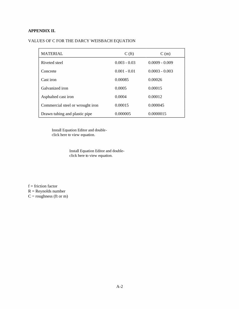
APPENDIX II. VALUES OF C FOR THE DARCY WEISBACH EQUATION

MATERIAL

C (ft)

C (m)

Riveted steel

0.003 - 0.03

0.0009 - 0.009

Concrete

0.001 - 0.01

0.0003 - 0.003

Cast iron

0.00085

0.00026

Galvanized iron

0.0005

0.00015

Asphalted cast iron

0.0004

0.00012

Commercial steel or wrought iron

0.00015

0.000045

Drawn tubing and plastic pipe

0.000005

0.0000015

f = friction factor R = Reynolds number C = roughness (ft or m)



A-3

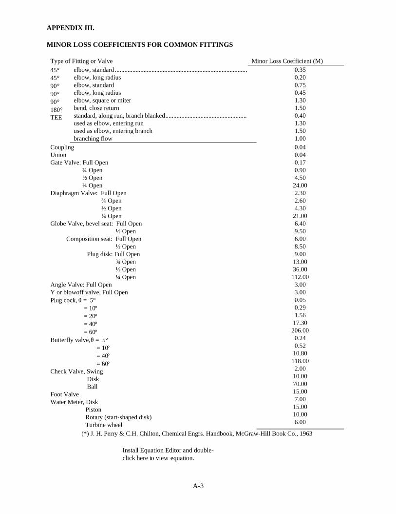
APPENDIX III. MINOR LOSS COEFFICIENTS FOR COMMON FITTINGS

Type of Fitting or Valve Minor Loss Coefficient (M)

45° 45° 90° 90° 90° 180° TEE

elbow, standard ................................................................................... elbow, long radius elbow, standard elbow, long radius elbow, square or miter bend, close return standard, along run, branch blanked ................................................... used as elbow, entering run used as elbow, entering branch branching flow

0.35 0.20 0.75 0.45 1.30 1.50 0.40 1.30 1.50 1.00

Coupling Union Gate Valve: Full Open ¾ Open ½ Open ¼ Open Diaphragm Valve: Full Open ¾ Open ½ Open ¼ Open Globe Valve, bevel seat: Full Open ½ Open Composition seat: Full Open ½ Open Plug disk: Full Open ¾ Open ½ Open ¼ Open Angle Valve: Full Open Y or blowoff valve, Full Open Plug cock, θ = 5° = 10° = 20° = 40° = 60° Butterfly valve, θ = 5° = 10° = 40° = 60° Check Valve, Swing Disk Ball Foot Valve Water Meter, Disk Piston Rotary (start-shaped disk) Turbine wheel

0.04 0.04 0.17 0.90 4.50

24.00 2.30 2.60 4.30

21.00 6.40 9.50 6.00 8.50 9.00

13.00 36.00 112.00

3.00 3.00 0.05 0.29 1.56

17.30 206.00

0.24 0.52

10.80 118.00

2.00 10.00 70.00 15.00 7.00

15.00 10.00 6.00

(*) J. H. Perry & C.H. Chilton, Chemical Engrs. Handbook, McGraw-Hill Book Co., 1963


A-4





Install Equation Editor and double-click here to view equation. Install Equation Editor and double-click here to view equation.


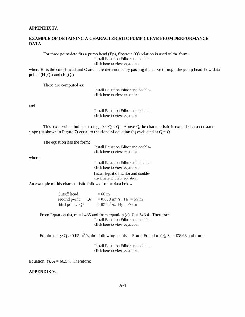
APPENDIX IV. EXAMPLE OF OBTAINING A CHARACTERISTIC PUMP CURVE FROM PERFORMANCE DATA

For three point data fits a pump head (Ep), flowrate (Q) relation is used of the form: where H is the cutoff head and C and n are determined by passing the curve through the pump head-flow data points (H ,Q ) and (H ,Q ).

These are computed as: and

This expression holds in range 0 < Q < Q . Above Q3 the characteristic is extended at a constant slope (as shown in Figure 7) equal to the slope of equation (a) evaluated at Q = Q .

The equation has the form: where

An example of this characteristic follows for the data below:

Cutoff head = 60 m second point: Q2 = 0.058 m3 /s, H2 = 55 m third point: Q3 = 0.ll5 m3 /s, H3 = 46 m

From Equation (b), m = l.485 and from equation (c), C = 343.4. Therefore:

For the range Q > 0.ll5 m3 /s, the following holds. From Equation (e), S = -l78.63 and from

Equation (f), A = 66.54. Therefore: APPENDIX V.


A-5

FORMULATION AND SOLUTION OF SYSTEM EQUATIONS Basic Equations

Pipe network equations for steady state analysis have been commonly expressed in two ways. Equations which express mass continuity and energy conservation in terms of the discharge in each pipe section have been referred to as loop equations and this terminology will be followed here. A second formulation which expresses mass continuity in terms of the HGL at junction nodes produces a set of equations referred to as node equations. It has been shown that the loop equations have superior convergence characteristics and these relationships are utilized in this program (1). Loop Equations

Equation (l) which defines the relationship between the number of pipes, primary loops, junction nodes

and fixed grade nodes offers a basis for formulating a set of hydraulic equations to describe a connected pipe

system. In terms of the unknown discharge in each pipe, a number of mass continuity and energy conservation

equations can be written equaling the number of pipes in the system. For each junction a continuity relationship

equating the flow into the junction (Q ) to the flow (Q ) is written as:

Qin - Qout = Qe (j equations) (Al)

Here Q represents the external inflow or demand at the junction node. For each primary loop the energy

conservation equation can be written for pipe sections in the loop as follows:

ΣhL = ΣEp (l equations) (A2)

hL = energy loss in each pipe (including minor loss)

Ep = energy put into the liquid by a pump.

If there are no pumps in the loop then the energy equation states that the sum of the energy losses around the loop equals zero.

If there are f fixed grade nodes, f - 1 independent energy conservation equations can be written for

paths of pipe sections between any two fixed grade nodes as follows:

∆E = Σh - ΣE (f - l equations) (A3)

where ∆E is the difference in the fluid energy (HGL) between the two fixed grade nodes. Any connected path of pipes within the pipe system can be chosen between these nodes. When identifying these f - l energy equations care must be taken to avoid redundant paths. The best method to avoid this difficulty is to either choose all parallel paths starting at a common node (like A-B, A-C, A-D, etc.) or to use a series arrangement where the previous ending node for a path is the starting node for the next path (like A-B, B-C, C-D, etc.). Either of these methods will result in f - l equations with no redundancy. The program employs the first scheme.

As an additional generalization, Equation (A2) can be considered to be a special case of Equation (A3) where the difference in fluid energy, ∆E, is zero for a path which forms a closed loop. Thus, the energy conservation relationships for pipe networks are expressed by l + f - l path equations of the form given by Equation (A3). The junction and path equations constitute a set of p simultaneous non-linear algebraic

A-6

equations referred to as loop equations. A steady state flow analysis based on the loop equations requires the solution of this set of equations for the flowrate in each line. To do this the path equations must be expressed in terms of the flowrate which is done as follows.

The energy loss in a pipe (h ) is the sum of the line loss (h ) and the minor loss (h ). The line loss expressed in terms of the flowrate is given by:

hLP = Kp Qn (A4) where K is a pipe line constant which is a function of line length (L), diameter (D), and roughness (C), or friction factor (f), and n is an exponent. The values of K and n depend on the energy loss expression used for the analysis.

For the Hazen Williams Equation

Kp = XL/C1.852 D4.87 (A5) and the exponent n = l.852. The constant X depends on the units used and has value X = 4.73 for English units and l0.675 for S.I. units.

For Darcy Weisbach Equation

Kp = 8 fL/gD5 π2 and the exponent n = 2.

The minor loss in a pipe section (hLM) is given as:

hLM = KM Q2 (A6) where K is a function of the sum of the minor loss coefficients for the fittings in the pipe section (ΣM) and the pipe diameter and is given by:

0.02517 ΣM/D4 (English units) and

0.08265 ΣM/D4 (S.I. units) (A7)

For pumps described by the useful power input the pump energy term (Ep ) is given by:

Ep = Z/Q (A8) where Z is a function of the useful power of the pump (Pu) and the relative density of the liquid (S) and is:

Z = 8.8l4 Pu /S (English units) (A9)

Z = 0.l0l97 Pu /S (S.I. units)

If the pump is described by operating data, the in range operation is described by:

A-7

Ep = H1 + C Qm (Al0)

Utilizing Equations (A4) - (Al0), the path (energy) equations expressed in terms of the flowrate are:

∆E = Σ (Kp Qn + Km Q2 ) - ΣZ/Q

or

∆E = Σ (Kp Qn + KM Q2 - Σ(H1 + C Q m) (All)

The continuity equations (Equation Al) and the energy equation (Equation All) form the set of p simultaneous equations in terms of unknown flowrates which are labeled the loop equations. Since these are non-linear algebraic relationships no direct solution is possible. Several algorithms for solving the loop equations have been developed. Of these the simultaneous path method is the most reliable and efficient for micro-computers and is employed in this computer model. Algorithm for the Solution of the Loop Equations - Enhanced Linear

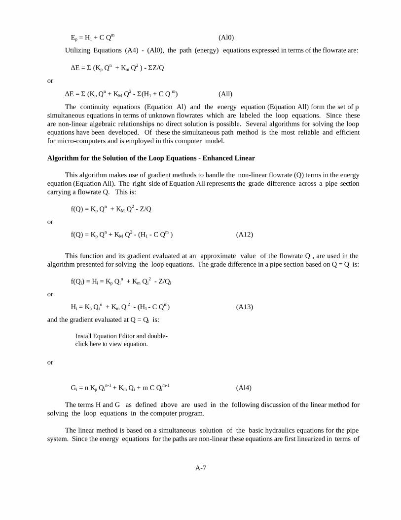
This algorithm makes use of gradient methods to handle the non-linear flowrate (Q) terms in the energy equation (Equation All). The right side of Equation All represents the grade difference across a pipe section carrying a flowrate Q. This is:

f(Q) = Kp Qn + KM Q2 - Z/Q

or

f(Q) = Kp Qn + KM Q2 - (H1 - C Qm ) (A12)

This function and its gradient evaluated at an approximate value of the flowrate Q , are used in the

algorithm presented for solving the loop equations. The grade difference in a pipe section based on Q = Q is:

f(Qi) = Hi = Kp Qin + Km Qi

2 - Z/Qi

or

Hi = Kp Qin + Km Qi

2 - (H1 - C Qm) (A13)

and the gradient evaluated at Q = Q1 is:

or

Gi = n Kp Qin-1 + Km Qi + m C Qi

m-1 (Al4)

The terms H and G as defined above are used in the following discussion of the linear method for solving the loop equations in the computer program.

The linear method is based on a simultaneous solution of the basic hydraulics equations for the pipe system. Since the energy equations for the paths are non-linear these equations are first linearized in terms of


A-8

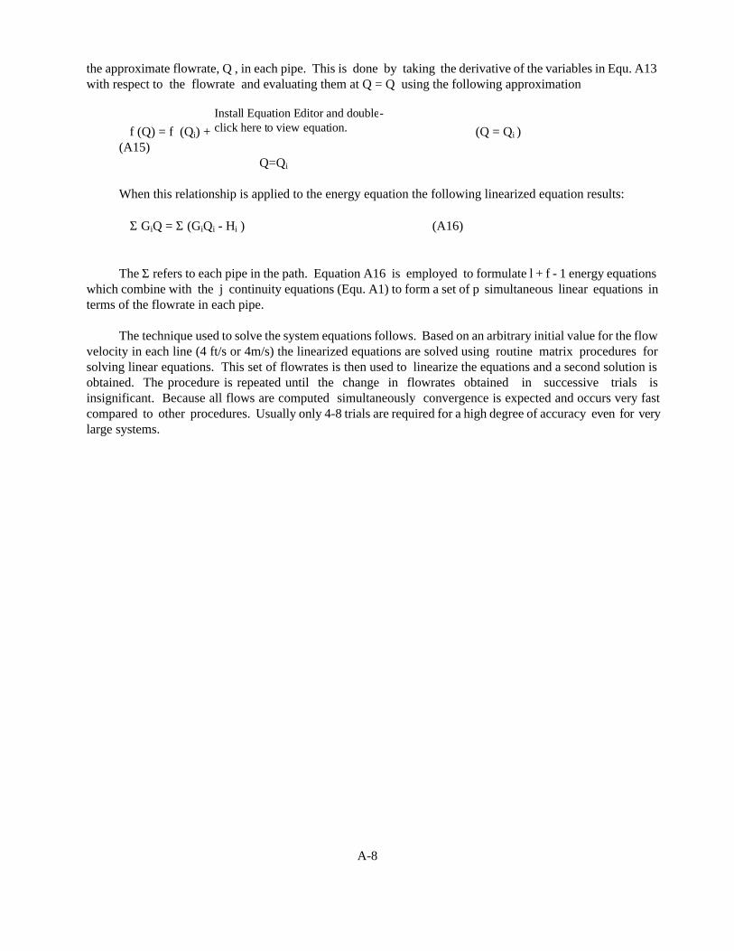
the approximate flowrate, Q , in each pipe. This is done by taking the derivative of the variables in Equ. A13 with respect to the flowrate and evaluating them at Q = Q using the following approximation

f (Q) = f (Qi) + Install Equation Editor and double-click here to view equation. (Q = Qi )

(A15) Q=Qi

When this relationship is applied to the energy equation the following linearized equation results:

Σ GiQ = Σ (GiQi - Hi ) (A16)

The Σ refers to each pipe in the path. Equation A16 is employed to formulate l + f - 1 energy equations which combine with the j continuity equations (Equ. A1) to form a set of p simultaneous linear equations in terms of the flowrate in each pipe.

The technique used to solve the system equations follows. Based on an arbitrary initial value for the flow velocity in each line (4 ft/s or 4m/s) the linearized equations are solved using routine matrix procedures for solving linear equations. This set of flowrates is then used to linearize the equations and a second solution is obtained. The procedure is repeated until the change in flowrates obtained in successive trials is insignificant. Because all flows are computed simultaneously convergence is expected and occurs very fast compared to other procedures. Usually only 4-8 trials are required for a high degree of accuracy even for very large systems.

A-9

APPENDIX VI DATA PREPARATION FORM - KYPIPE2 1a. SYSTEM DATA

Simulation type key (1 for EPS) ................................................................................................. = ______

Number of pressure constraints .................................................................................................. = ______

Flow identification key (0-CFS, 1-GPM, 2-MGD, 3-L/S, 4-CMS) .......................................... = ______

Number of pipes .......................................................................................................................... = ______

Number of junction nodes ........................................................................................................... = ______

Number of regulating valves ....................................................................................................... = ______

*Maximum number of trials (default-40) .................................................................................. = ______

*Relative accuracy (default-.005) .............................................................................................. = ______

*Specific gravity (default-1.0) ................................................................................................... = ______

*Kinematic viscosity (default-HW equ.) ................................................................................... = ______

*Print junction titles ................................................................................................................... = ______

*Non consecutive pipe numbering ............................................................................................ = ______

*Omit this data to use program defaults

* * * * * * 16. PIPE COST DATA

Diameter

Type (0-9)

Unit Cost

A-10

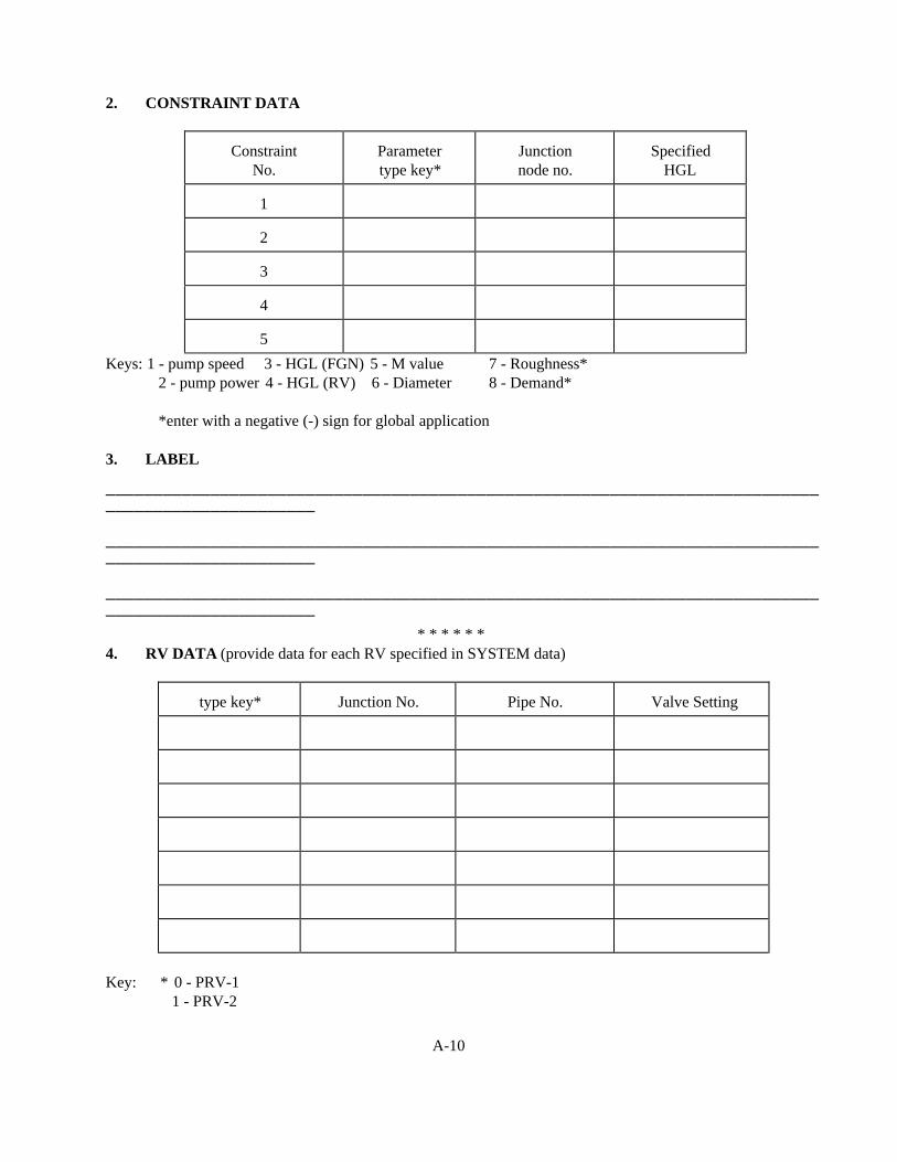
2. CONSTRAINT DATA

Constraint

No.

Parameter type key*

Junction node no.

Specified

HGL

1

2

3

4

5

Keys: 1 - pump speed 3 - HGL (FGN) 5 - M value 7 - Roughness*

2 - pump power 4 - HGL (RV) 6 - Diameter 8 - Demand*

*enter with a negative (-) sign for global application 3. LABEL

───────────────────────────────────────────────────────────────────────────────────────────────── ───────────────────────────────────────────────────────────────────────────────────────────────── ───────────────────────────────────────────────────────────────────────────────────────────────── * * * * * * 4. RV DATA (provide data for each RV specified in SYSTEM data)

type key*

Junction No.

Pipe No.

Valve Setting

Key: * 0 - PRV-1

1 - PRV-2

A-11

2 - PSV 3 - FCV-1 4 - FCV-2

5. PIPE DATA (one line for each pipe)

Status Code

Node No. 1

Node No. 2

Length

Diam

Roughness

Minor Loss

Pump Data

FGN HGL

* T

* * C

Pipe No. 9

A-12

* Pipe Type (0-9) - Enter this data for auxiliary applications (cost, calibration, water quality) ** Constraint Data - Enter constraint number if parameter for this pipe is to be determined 6. PUMP DATA (for pumps described by operating data)

Pipe Numbers

Cutoff head (HC)

efficiency (optional)

Q1 (or 0)

H2

Q2

H3

Q3

Identifier no. (ID)

*No. additional data (AD)

Pump speed (n) (defaults to 1)

* Enter this number of head-flow data points following the above data (in order of ascending flowrate). * Additional Pump Data (maximum of 8 points)

head

flow

A-13

7. JUNCTION DATA (data must be provided if flow demand present - otherwise optional)

Demand **

Elevation

*

CD

Junction

No.

Demand

Type ***

* Constraint Data - Enter Constraint number if demand is to be calculated. ** Use flow units previously specified. *** Defaults to 1 (enter only higher demand types)

A-14

BLANK LINE (end of junction data)

A-15

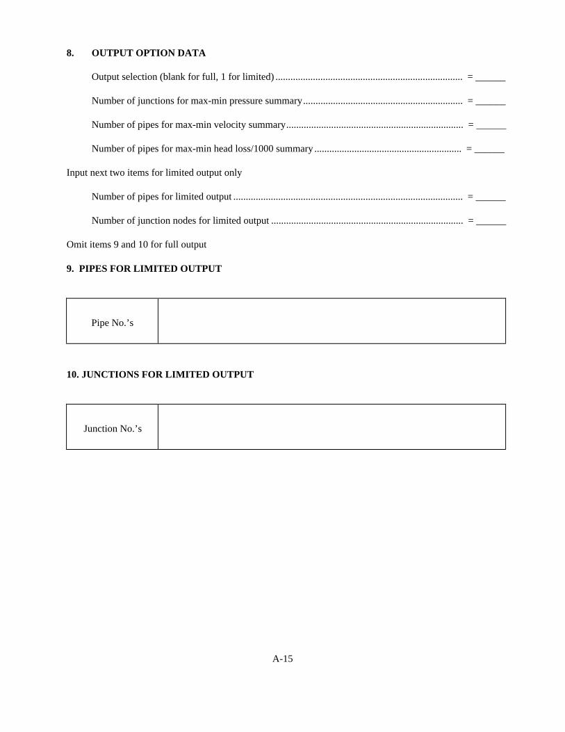
8. OUTPUT OPTION DATA

Output selection (blank for full, 1 for limited) ........................................................................... = ______

Number of junctions for max-min pressure summary ................................................................ = ______

Number of pipes for max-min velocity summary ....................................................................... = ______

Number of pipes for max-min head loss/1000 summary ........................................................... = ______ Input next two items for limited output only

Number of pipes for limited output ............................................................................................ = ______

Number of junction nodes for limited output ............................................................................. = ______ Omit items 9 and 10 for full output 9. PIPES FOR LIMITED OUTPUT

Pipe No.’s

10. JUNCTIONS FOR LIMITED OUTPUT

Junction No.’s

A-16

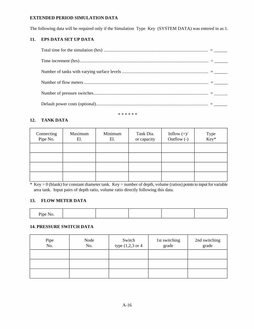
EXTENDED PERIOD SIMULATION DATA The following data will be required only if the Simulation Type Key (SYSTEM DATA) was entered in as 1. 11. EPS DATA SET UP DATA

Total time for the simulation (hrs) ............................................................................................. = ______

Time increment (hrs) ................................................................................................................... = ______

Number of tanks with varying surface levels ............................................................................. = ______

Number of flow meters ............................................................................................................... = ______

Number of pressure switches ...................................................................................................... = ______

Default power costs (optional).................................................................................................... = ______

* * * * * * 12. TANK DATA

Connecting

Pipe No.

Maximum

El.

Minimum

El.

Tank Dia. or capacity

Inflow (+)/ Outflow (-)

Type Key*

* Key = 0 (blank) for constant diameter tank. Key = number of depth, volume (ratios) points to input for variable area tank. Input pairs of depth ratio, volume ratio directly following this data.

13. FLOW METER DATA

Pipe No.

14. PRESSURE SWITCH DATA

Pipe No.

Node No.

Switch

type (1,2,3 or 4

1st switching

grade

2nd switching

grade

A-17

15. CHANGES SPECIFIED

** Time for these changes (only for EPS) ................................................................................ = ______

a) Number of junction nodes - demand changes.......................................................................... = ______

b) Number of open-closed pipe status changes ........................................................................ = ______

Global roughness addition factor (default = 0) .................................................................... = ______

Global roughness multiplication factor (default = 1) .......................................................... = ______

GDF1 (default = 1) .............................................................................................................. = ______

GDF2 (default = 1) .............................................................................................................. = ______

GDF3 (default = 1) .............................................................................................................. = ______

GDF4 (default = 1) .............................................................................................................. = ______

** Time interval for EPS calculations (change only) ............................................................... = ______

c) ** Number of tanks - external inflows changed ...................................................................... = ______

d) Power cost change - effective at this time (optional) ........................................................... = ______

** This data requested (or required) only for EPS

* * * * * *

LABEL (optional) ───────────────────────────────────────────────────────────────────────────────────────────────── ───────────────────────────────────────────────────────────────────────────────────────────────── ─────────────────────────────────────────────────────────────────────────────────────────────────

* * * * * *

Provide the following data for the number of changes specified above: a) JUNCTION DEMAND CHANGES

Junction No.

New Demand

* * * * * *

b) PIPES OPEN CLOSED STATUS CHANGE

Pipe No.

A-18

c) EXTERNAL TANK FLOWS

Tank No.

External Flow + in, - out

PIPE PARAMETER CHANGE DATA I provide the following data for each pipe with data changes

pipe number

length

diameter

roughness

minor loss

pump data

II provide the following for each HGL change for FGN's

pipe no. (must connect FGN)

new HGL

A-19

APPENDIX VI SIZE Program

In Section 8 four alternatives were noted for determining pipe diameters utilizing results which do not represent available diameters. These alternatives are listed below and depicted in a schematic. Not all of these alternatives are feasible for some situations.

1. Select the next largest nominal diameter. 2. Determine the length of sections of a series pipe of

the next smallest and next largest nominal pipe equivalent to the calculated diameter, D.

3. Determine the smallest nominal diameter of a pipe parallel to the original pipe which provides a capacity equal or greater than Dc.

4. Determine lengths of a series pipe installed parallel to the original pipe with a capacity equal to Dc.

A program called SIZE is provided to enable you to evaluate these options for a particular result. This program selects diameters from a table of available diameters for the alternative designs. You can add or delete items from this table. You then provide required basic data and the calculations are carried out. An example run is shown below for the first results obtained with Example 5C.

To access SIZE get the DOS prompt and type SIZE. You then respond to screen prompts as shown.

****** TABLE OF NOMINAL DIAMETERS ****** 1.00

2.00

3.00

4.00

6.00

8.00

10.00

12.00

14.00

15.00 16.00

18.00

21.00

24.00

30.00

36.00

42.00

48.00

60.00

72.00 84.00

96.00

DO YOU WANT TO A) DD OR D) ELETE A DIAMETER OR C) ONTINUE

Enter Data to Carry Out Pipe Diameter Calculations

Original Length

=

?

2100

Original Diameter =

?

10

Original C Value =

?

120

Design C Value =

?

130

Calculated Diameter =

?

11.67

********** PIPE SIZE ANALYSIS *********** design

calc. diameters

series pipe

parallel pipe

(parallel-series)

HW-C

DC

DA

DN

DN-1

LN

LN-1

DC

DN

DN-1

LN

LN-1 130

11.67

11.32

12.00

10.00

1618

482

7.45

8.00

6.00

2100

284

Do you want to do another case (Y or N) ? N

A-20

APPENDIX VIII KYPIPE2 Modeling Notes Leak Pipes

It is sometimes desirable to model potential leakage from a network. This can be done by connecting pipes which usually have a high resistance to a FGN. These pipes are connected to the network at selected nodes. The pipes can be sized to provide a specified leakage for a specified conditions. The modeled leakage rates will then vary as the pressure (or hydraulic grade) in the network varies in much the same manner that actual leakage rates would be expected to vary with pressure. Leak pipes can also be used to avoid problems associated with excessive pump and regulating valve switching which are sometimes encountered. This application is discussed in the next section.

To set up a leak pipe you need only to add a pipe to your data which connects a selected node to a FGN. The rate of leakage will depend on the data you specify for the leak pipe. To specify a particular leakage rate, you should select all the characteristics of the pipe except one (normally diameter) and then calculate the remaining one. For example, to set up a leak pipe which will provide 10 gpm of leakage for a pressure drop of 40 psig (92.3 ft.), you can select a length and roughness and calculate the diameter from

where D is the pipe diameter (inches), L is the length assigned to the leak pipe (feet), Q is the leak rate in CFS and C is the assigned Hazen Williams roughness. If you assign L = 100 feet and C = 100, you should calculate D = .69 inches. You also must set the FGN grade for the leak pipe at about 92.3 feet below the node grade for the selected conditions.

Because of the small diameters which are normally used with leak pipes, it is possible that some inaccurate calculations may result in the grades in the vicinity of the node connecting the leak pipe. Specifying a higher accuracy will usually eliminate these. Also, adding leak pipes at the end of the pipe data is recommended. If the diameters used are too small, it may not be possible to totally eliminate the effect on a few grade calculations. However, all flowrates and other grades will be calculated with a high degree of accuracy. Using Leak Pipes to Avoid Modeling Problems

With the current KYPIPE2 state-of-the-art modeling capabilities a great deal of switching is possible. Regulating valves, pumps, pressure switches and storage tanks can all switch from on to off. If during a simulation a section of pipes with no open connection to a supply becomes isolated, a solution may not be possible and a fix is attempted. This may not be successful or acceptable. Adding a leak pipe to areas which become isolated will avoid these problems and this action is recommended if you encounter such a problem.

We have noted that several users are modeling supplies which include pumps and pressure regulating valves in series and may introduce conditions where this supply is closed causing both the


A-21

regulating valve and the pump to shutdown. This isolates the region between the two and can cause a modeling problem. Since the network hydraulics depends only on the pressure maintained by the regulating valve it is normally not necessary to model the pump. Setting up the situation can be simplified by representing the PRV as a fixed grade node operating at the set pressure as shown below and we normally recommend this approach. However, if the PRV is expected to operated abnormally (wide open or closed) then you may wish to include the pump in your model. If shutdown of this supply is possible then you should introduce a leak pipe between the pump and PRV as illustrated below, the problem noted previously may be avoided. The effect of a properly selected leak pipe is very small.

We have tested a variety of complex models and have found that any modeling problems which were encountered due to switching can be avoided by adding one or more leak pipes.

Our experience is that KYPIPE2 can model any network situation which is physically possible. There are, of course, a few situations which are not feasible and can not be modeled. For example, you can set up a pressure switch which can not possibly work. Suppose you set a booster pump to switch on when a node pressure is below a certain value and off when the pressure exceeds a second value. If the pump off produces a pressure value below the lower switch and the pump on produces a pressure value above the higher switch, then no acceptable solution exists. KYPIPE2 will flag the excessive switching and you will need to modify your data. If you run into a modeling problem, contact us for technical support and we can probably sort out the problem.

A-22

APPENDIX XIII COMPUTER ERROR DETECTION AND WARNINGS

Error Messages

KYPIPE performs a number of checks of geometric conditions and other data input are made and a message is produced if an error is detected. PIPEDATA will also identify a number of errors and the PIPEDATA data check operation should be employed on all KYPIPE data files. The PIPEDATA error messages and warnings are described in Appendix VI (Attachment A). The following is a list of messages which are a result of a condition which makes an analysis impossible and execution termination results. The probable cause of this situation and the action required to correct the error is discussed. Some examples are cited. 1. A PORTION OF THE SYSTEM IS DISCONNECTED BY CLOSED LINES FROM A

FGN. This message means that part of the system has no connection to a FGN which is not acceptable and is probably caused by incorrect input data for connecting nodes or, perhaps, the omission of a pipe. The input data summary should be checked and the data corrected. In most situations a fix will be made so a hydraulic analysis can proceed.

2. THE INPUT FOR PIPES CONNECTING JUNCTION - DO NOT CHECK (*3). This

message is produced if the geometric verification option (*3) is employed and the data input for connecting pipes at the indicated junction node does not check the data generated from connecting node input. It should be a simple matter to locate the data discrepancy indicated by this message. Note that the list of connecting pipes for each node printed by KYPIPE is generated based on the connecting nodes input for pipes and this is compared to your input for each junction node.

3. THE RELATIONSHIP P = J + L + F - 2 IS NOT SATISFIED - CHECK INPUT DATA.

Loop and path data are generated by the computer using the connecting node data input for the pipes. If this basic geometric relationship is not satisfied after generation of the loop and path data this message is generated. It is likely that one of the earlier messages concerning connecting node data will also be generated if this condition occurs. The input data summary must be checked, particularly the connecting pipes of junction nodes, and the data corrected.

4. THE SYSTEM EQUATIONS CANNOT BE SOLVED. This message is produced if the

basic equations cannot be solved in the subroutines. The situation could be caused by some bad data (such as a zero value for a diameter) or by exceeding dimensions. A data change or a dimension change is required to correct this problem. If pressure constraints are defined this problem will normally be a result of a non feasible situation and an additional message will appear. The constraint data should be modified such that a feasible condition is possible.

5. ALL PIPES CONNECTING JUNCTION - ARE CLOSED - INPUT DATA MUST BE

CORRECTED. The data which causes this condition must be corrected before an analysis can be made. KYPIPE will attempt to fix this problem by setting the demand to zero at the junction and opening one of the connecting pipes.

A-23

6. THE NUMBER INPUT FOR THIS PIPE HAS BEEN PREVIOUSLY ASSIGNED. This message indicates that the number read in for a pipe using the non-consecutive numbering option (*9*) has been previously used and this data must be corrected.

7. DATA IS INPUT FOR JUNCTION NODE - WHICH IS NOT USED IN THE PIPE DATA.

This message is generated when the junction node input data is specified for a junction node which was not used in the pipe data. The data must be corrected to eliminate this situation.

8. INAPPROPRIATE INPUT DATA HAS PRODUCED A CONDITION WHICH IS

UNACCEPTABLE. This message may result from a number of data errors including:

a) An assigned pipe or junction node number exceeds the allowable limit. b) In an EPS a normal time period of zero is specified. c) In an EPS the time specified for the next change is inappropriate.

The specified time may be less than the time previously reached or the specified time will not be used in the simulation. (Changes must be specified at times used to carry out the simulation.)

d) In an EPS excessive oscillation in tanks is occurring indicating that the system data is not suitable.

e) For changes, a pipe or junction node is specified, and this number is not used in the original data.

If this message appears it will be possible in most cases to review the Output file and locate approximately where in the data set the problem occurs and correct the data.

9. PUMP DATA FOR LINE - IS NOT SUITABLE. The head-flow data is input in the incorrect

order or the flowrates are not input in descending order. The program will not accept this data and it must be changed.

10. DATA HAS NOT BEEN ENTERED FOR PUMP TYPE ____. This error appears if you use

a pump type ID in the input data without defining the head-flow data points and this data was not entered previously.

11. THIS PIPE IS DESIGNATED AS CONNECTING AN RV AT NODE ____. The pipe data

is inconsistent with the RV data previously input. 12. NO PIPES OR JUNCTIONS ARE DESIGNATED FOR CONSTRAINT NO. ____. This

constraint was defined in the Constraint Data but was not associated with any specific pipes or nodes as required for all constraints.

13. CONSTRAINT NO. ____ IS NOT CORRECTLY ASSOCIATED. This means that the

parameter associated with the constraint is not acceptable. The most common cause of this problem is that the designated pipes are in a branched area where the terminating node is not pressure constrained.

14. THIS IS A NON FEASIBLE SITUATION - MODIFY THE CONSTRAINT DATA. This

message appears if a singular matrix is generated or a convergence failure occurs.

A-24

15. EPS SIMULATION TERMINATED - EXCESSIVE CHANGES DURING TIME PERIOD. TRY USING A SMALLER TIME INCREMENT FOR THIS TIME PERIOD. Due to excessive tank filling or emptying or excessive operation of pressure switches a high number of simulations are required during a single time period. This could indicate an incorrect pressure switch setup. When this reaches a set limit the run is aborted.

16. SIMULATION TERMINATED. AN ERROR WAS DETECTED OR YOU REQUESTED A

DATA CHECK OPTION (*1). This message will be generated if a data check (option *1*) is specified or if certain other errors are detected. In most cases other errors will be identified in a previous message.

Additional Computer Messages and Warnings

A number of other messages may be generated which alert you to various situations. These

messages and their implications are discussed here. 1. A SUCCESSFUL GEOMETRIC VERIFICATION HAS BEEN COMPLETED. This message

appears upon successful completion of the geometric verification option (*3*) and should assure you that your system is geometrically input correctly. This message occurs in the output for Examples 3 and 8.

2. THE PUMP IN LINE ___ IS OPERATING OUT OF RANGE. This message alerts you to

the fact that the pump indicated is operating below the lower limit or above the maximum discharge defined within the normal operating range. Example 3 illustrates this situation. This result may be acceptable or you may wish to carry out another analysis with the pump characteristics redefined. This message will only be produced when the pump is described by operating data.

3. WARNING - THE MAXIMUM NUMBER OF TRIALS WERE EXECUTED - ACCURACY

WAS NOT ATTAINED. This message indicates that a convergence problem has occurred and more trials are required or some input data is incorrect and must be redefined. The results and accuracy reached will be output so you can judge whether additional trials are required. This may be caused by check valves operating very close to zero flow or PRV's adjusting between a wide opened and throttled position. This condition can also be caused by great differences in pipeline parameters (diameters and roughnesses) which could denote incorrect input.

4. WARNING - PIPE DIAMETERS LESS THAN .5 MAY CAUSE CONVERGENCE OR

ACCURACY PROBLEMS. This message indicates that a small diameter (<.5) has been input and this data may cause difficulties.

5. WARNING - A PIPE PARAMETER HAS BEEN ASSIGNED A VALUE OF ZERO -

CORRECT THIS DATA. Diameter, lengths, and roughnesses must have a non-zero value and if the input data does not assign a non-zero value this message is generated.

6. WARNING - EXCESSIVE REGULATING VALVE ADJUSTMENTS -

ADJUSTMENTS TERMINATED. CHECK TABULATED RESULTS FOR REGULATING VALVES. This message indicates that excessive trials are required to determine the operating status of regulating valves and the calculations are proceeding

A-25

without further adjustments. You should review the Regulating Valve Report to determine the status of the regulating valves. The problem may be due to one or more valves operating very close to the limit defining two modes of operation.

7. WARNING - A HEAD INCREASE OF ____ IS REQUIRED FOR PIPE ____. This

message occurs when you have called for a calculation of the minor loss coefficient when actually a head increase is required to meet the constrained pressure.

8. WARNING - FLOW REVERSED IN CONSTRAINED PUMP LINE. This message means

that flow reversal in a line containing a pump is required to meet the constrained pressure. 9. WARNING - SOLUTION FOR CONSTRAINT NO. ____ IS NOT FEASIBLE. A

NEGATIVE FACTOR WAS OBTAINED FOR DIAMETER (OR ROUGHNESS). This means that an energy gain is required to meet the constrained pressure and a calculation of diameter (or roughness) is not feasible.

10. WARNING - THE NUMBER OF JUNCTION NODES = ___ WHICH DOES NOT AGREE

WITH INPUT DATA. The computer cannot verify the number of junction nodes specified on the SYSTEM DATA card. The simulation will continue the simulation using the number of junction nodes determined by the computer.

A-26

APPENDICES APPENDIX I Values of C for Hazen Williams .................................................................................. A-01 APPENDIX II Valves of ε for Darcy Weisbach ......................................................................................... A-02 APPENDIX III Minor Losses Coefficient for Common Fittings................................................................. A-03 APPENDIX IV Example of Obtaining Characteristic Pump Curve ............................................................ A-04 APPENDIX V Formulation and Solution of System Equations ................................................................. A-05 APPENDIX VI DATA PREPARATION FORMS ...................................................................................... A-17 APPENDIX VII SIZE Program ..................................................................................................................... A-37 APPENDIX VIII Leak Pipes .................................................................................................................... A-38 APPENDIX IX Computer Error Detection and Warnings ........................................................................... A-38

kypipe appendix

Documents