l. a. karoly, c. schröder - pe.cemi.rssi.rupe.cemi.rssi.ru/pe_2015_1_125-138.pdf · the paper...

L. A

. Kar

oly

, C. S

chrö

der

125

Applied econometrics ПРИКЛАДНАЯ ЭКОНОМЕТРИКА

Theory and methodology Теория и методология

№ 37 (1) 2015

L. A. Karoly, C. Schröder

Fast methods for jackknifing inequality indices

The jackknife is a resampling method that uses subsets of the original database by leaving out one observation at a time from the sample. The paper develops fast algorithms for jack-knifing inequality indices with only a few passes through the data. The number of passes is independent of the number of observations. Hence, the method provides an efficient way to obtain standard errors of the estimators even if sample size is large. We apply our method using micro data on individual incomes for Germany and the US.Keywords: jackknife; resampling; sampling variability; inequality.

JEL classification: C81; C87; D3.

1. Introduction

W hen examining time-series changes in inequality or cross country differences in inequal-ity, the measured changes are sometimes small. The delta method, bootstrapping and jackknifing are popular methods for performing statistical inference on inequality indi-

ces. The delta method is based on the asymptotic distribution of the index, whereas the jackknife and the bootstrap are distribution free resampling methods. The bootstrap samples with replace-ment from the original sample1. The jackknife uses subsets of the original database by leaving out one observation at a time from the sample2.

The delta method, if applicable to an inequality index, has as advantages that it derives the asymptotic distribution using the central limit theorem, and that the computational burden to estimate the asymptotic variance consistently is low. However, the delta method is not free of limitations. For example, one difficulty arises if cross-sections of a panel survey are used as the empirical database, as it is the case for available micro datasets including the Luxembourg Income Study (LIS)3, probably the most frequently used database for distributional analyses worldwide. Then for testing for inter-temporal changes in inequality indices the inter-temporal covariance structure of incomes must be considered. Further difficulties arise in the following contexts (see (Heshmati, 2004), and references therein for details): correlated data, correlations introduced in error terms4, panel attrition, and inequality decomposition5.

1 For the validity of the bootstrap technique in inequality analyses see (Biewen, 2002).2 For the theoretical justification for the jackknife and other related resampling techniques see (Efron, 1982).3 http://www.lisdatacenter.org/.4 Modarres and Gastwirth (2006) show that regression estimates of the standard error for the Gini index can be

biased «as it does not account for the correlation introduced in the error terms once the data are sorted» (p. 387).5 Decomposition analyses impose restrictions on the functional forms of regression models (see (Fields, Yoo, 2000),

or (Morduch, Sicular, 2002)).

126 Теория и методология Theory and methodology

ПРИКЛАДНАЯ ЭКОНОМЕТРИКА Applied econometrics№ 37 (1) 2015

Aforementioned limitations of the delta method explain the interest in resampling methods6. The central advantage of the jackknife over other resampling methods such as the bootstrap is that it allows the replication of results. A disadvantage of standard jackknife procedures is that for large sample sizes the computational burden is substantial. This is because there are as many subsets as there are observations in the sample, and for each subset the jackknife statistic needs to be computed. This paper offers a solution. We provide fast algorithms, requiring only a few passes through the data, for jackknifing several popular inequality indices: coefficient of varia-tion, variance of the logarithms, mean log deviation, Theil index, and Atkinson index7. Since the number of passes is independent of the number of observations, even for large samples the computational burden remains small.

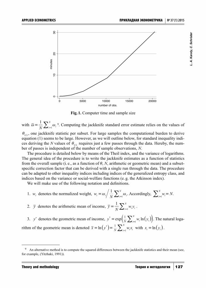
To get an idea of the computational burden see Fig. 1. It charts the computer time in minutes for a standard procedure for jackknifing inequality indices as a function of sample size8. Comput-er time increases exponentially in sample size, and for a sample size of about 80 000 cases it al-ready exceeds four hours. Since many comparative inequality analyses rely on data from several points in time, countries and income concepts, computing the jackknife for all results can easily take days or weeks. This is a serious limitation, especially for researchers who use data stored on external servers (e. g., the Luxembourg Income Study) and face limited processing power.

Section 2 explains our jackknife algorithm. Section 3 provides the results from an empirical application relying on data from the Luxembourg Income Study. Section 4 concludes. Deriva-tions of all the formulas are provided in an Appendix.

2. Efficient jackknife procedures for inequality indices

The jackknife offers a conceptually simple way to estimate the precision of a statis-tic, see the pioneering (Tukey, 1958; Efron, 1982; Efron, Gong, 1983; Wolter, 1985). In the context of inequality measurement, we have a random sample of N observations on income, y= ( , , , )y y yN1 2 and sampling weights, w w w1 2, , , N . Let θ θ= ( )y denote our measure of inequality. Let θ θ( ) , , , , , ,i i i Ny y y y y= ( )− +1 2 1 1 denote the jackknife estimate of the same mea-sure of inequality for the subset where the i-th observation has been deleted.

Following Wolter (1985), the jackknife estimate of the standard error of is

SENN

i

i

N

iθ

ω

ωθ θ=

−−

=( )∑1

1

20 5.

, (1)

6 For example, Biewen (2002) shows the validity of the bootstrap in a number of aforementioned contexts. Modarres and Gastwirth (2006) recommend bootstrap and jackknife as reliable methods for random samples as opposed to other methods that assume independence between errors when they are dependent (as it is the case for the Gini coefficient). Bhattacharya (2007) suggests techniques of asymptotic inference of the Gini coefficient based on process theory and the delta method. The resulting variance formula, however, is rather difficult to implement (Davidson, 2009).

7 Algorithms for the Gini coefficient are provided in (Karagiannis, Kovacevic, 2000) and (Yitzhaki, 1991). Karoly (1989) derives jackknife procedures for calculating the between- and within-group inequality components of the variance of the logarithms, the mean log deviation, and the Theil index. Ogwang (2000) shows that it is also possible to obtain standard errors for the Gini index from OLS regression. Giles (2004) extends the regression-based approach to test hypotheses regarding the sensitivity of the Gini coefficient to changes in the data using seemingly unrelated regressions.

8 We have used the STATA software package inequal7.ado on the following hardware: 64-bit system; 8 GB RAM; Core 2 Duo CPU, 3GHz. STATA code is available in the authors' working paper (Karoly, Schröder, 2014).

L. A

. Kar

oly

, C. S

chrö

der

127



№ 37 (1) 2015

with ω ω==

∑11N ii

N9. Computing the jackknife standard error estimate relies on the values of

θ( )i , one jackknife statistic per subset. For large samples the computational burden to derive equation (1) seems to be large. However, as we will outline below, for standard inequality indi-ces deriving the N values of θ( )i requires just a few passes through the data. Hereby, the num-ber of passes is independent of the number of sample observations, N.

The procedure is detailed below by means of the Theil index, and the variance of logarithms. The general idea of the procedure is to write the jackknife estimates as a function of statistics from the overall sample (i. e., as a function of , N, arithmetic or geometric mean) and a subset-specific correction factor that can be derived with a single run through the data. The procedure can be adapted to other inequality indices including indices of the generalized entropy class, and indices based on the variance or social-welfare functions (e. g. the Atkinson index).

We will make use of the following notation and definitions.

1. wi denotes the normalized weight, w Ni i ii

N=

=∑ω ω

11

. Accordingly, w Nii

N

=∑ =

1.

2. y denotes the arithmetic mean of income, yN

w yi ii

N=

=∑1

1.

3. y denotes the geometric mean of income, y w yN i ii

N* exp ln= ( )( )=

∑11

. The natural loga-

rithm of the geometric mean is denoted x y w xN i ii

N= ( )=

=∑ln * 1

1 with x yi i= ( )ln .

9 An alternative method is to compute the squared differences between the jackknife statistics and their mean (see, for example, (Yitzhaki, 1991)).

010

2030

min

utes

0 5000 10000 15000 20000number of obs.

Fig. 1. Computer time and sample size



2.1. Efficient jackknife procedure for the Theil index

The Theil index from the sample is

θT i i ii

N

N yw y y y= ( )

− ( )

=

∑1

1

ln ln . (2)

The Theil index for the subset where the i-th observation has been deleted is

θT ii i

j j jj i

iN w yw y y y( )

( )( )ln ln ,=

−( )( )

− ( )

≠

∑1 (3)

with y i( ) denoting the arithmetic mean of income from the subset

yN y w yN wi

i i

i( ) .=

−

− (4)

The first step is to write T i( ) in terms of T . Initially, from (3):

θT ii i

i i ii

Ni

i

i

iiN w y

w y yw

N wyy

y( )( )

ln ln=−( )

( )

−

−( )( )−

=

∑1

1

lln .( )y i( ) (5)

Rewriting equation (2) gives

w y y y N yi i ii

N

Tln ln( )= + ( ) =

∑1

θ , (6)

and substituting (6) and (4) into (5) gives

θ θT ii i

Ti i i

i i

i i

i

N yN y w y

yw y yN y w y

N y w yN w( ) ln

lnln=

−+ ( )( )−

( )−

−−

−

. (7)

Equation (7) reveals that T i( ) can be expressed as a function of three statistics from the full sample, N y, , and T , and characteristics of the observation that is left out, wi and yi. Thus, af-ter having calculated N y, , and T for the full sample, to compute all the jackknife statistics θ θT T N( ) ( )1 , , takes a single pass through the data.

2.2. Efficient jackknife procedure for the variance of logarithms

Applying Bessel’s correction10, the variance of the logarithms from the sample is

θVL ii

i

N

i ii

N

Nw

yy N

w x x=−

=

−−( )

= =

∑ ∑11

111

22

1

ln .* (8)

10 Bessel’s correction, the division in the variance formula by N - 1 instead of by N, secures unbiasedness.

L. A

. Kar

oly

, C. S

chrö

der

129



№ 37 (1) 2015

The variance of the logarithms for the subset where the i-th observation has been deleted is

θVL i j i j ij iNw x x( ) ( ) ( ) ,=

−−( )

≠

∑12

2 (9)

with xN w

NX x wii

i i( ) = −−[ ]1

, and with ww

N w Nj ij

i( ) /=

− −( ) ( )1 denoting re-weighted norma-

lized weights. By means of the re-weighting the average of wj i( ) over the subset where the i-th

observation has been deleted equals unity. So, the analogue of the term 1

1N- in (8) in (9) is

12N-. Substituting the definition of wj i( ) in (9) gives

θVL ii

j j ij i

NN N w

w x x( ) ( ) .=−( )

−( ) −( )−( )

≠

∑12

2 (10)

Initially, from (8):

θVL j jj i

i iNw x x

Nw x x=

−−( ) +

−−( )

≠

∑11

11

2 2. (11)

Substituting xN

N w x x wi i i i= −( ) + 1

( ) in (11) gives

θVL j j i i i ij i

i iNw x

NN w x x w

Nw x x=

−− −( ) +

+

−−( )

≠

∑11

1 11

2

( )22=

(12)

=−

− + −

≠

11

2

Nw x

NNx

wNx

wNxj j i

A

ii

ii

Bj i

( ) ( )� ��

∑∑ +−

−( )11

2

Nw x xi i .

Equation (12) can be rewritten as

θVL j j ij i

C

j j ii

Nw x x

Nw x x

wN

=−

−( ) +−( )

−( )≠

∑11

21

2

( ) ( )

� ��

−( )

+

+−

≠

∑ x x

Nw

wNx

i ij i

D

ji

i

( )

( )

� ��

11

−−

+

−−( )

≠

∑ wNx

Nw x xi

ij i

E

i i

221

1� ��

.

(13)

The C-term on the right hand side of (13) can be rewritten as θVL iiN N w

N( )

( )− −( )−( )21 2 .

The D-term is zero since

DN

wN

w x x x xw

N Nx x w x xi

j j i i ij i

ii i j j=

−−( ) −( )=

−( )−( ) −

≠

∑21

21( ) ( ) ( ) (( )i

j i

( )=≠

=

∑0

0� ��

. (14)



The E-term after some algebra becomes

EN

wN w

w x xN

wN w

N w x xi

ij i

j i

i

ii i=

− −( )−( ) =

− −( )−( ) −( ) =

≠

∑11

11

2

22

2

22

==− −

−( )11

22

Nw

N wx xi

ii .

(15)

Substituting (14)–(15) in (13), the variance of the logarithms for the sample becomes

θ θVL VL ii i

ii

ii

N N wN N

wN w

x xwN

x x=−( ) −( )

−( )+

− −−( ) +

−−( )( )

21

11 12

22 22

. (16)

After some algebra, (16) becomes

θ θVL VL ii i

ii

N N wN

NwN N w

x x=−( ) −( )

−( )+

−( ) −( )−( )( ) .

21 12

2 (17)

Solving (17) with respect to VL i( ) gives the desired expression for the jackknife estimator of

the variance of the logarithms:

θ θVL i VLi

i

ii

NN N w

Nw NN w N

x x( ) .=−( )

−( ) −( )−

−( )

−( ) −( )−( )1

21

2

2

22 (18)

Equation (18) is the analogue of the jackknife estimator of the Theil index in equation (7): VL i( ) can be expressed as a function of statistics from the full sample (N x, , and VL) and the characteristics of the observation that is left out, wi and xi . Thus, after having calculated N x, , and VL for the full sample, computing VL VL N( ) ( ), ,1 takes a single pass through the data.

2.3. Efficient jackknife procedure for other inequality indices

Similar derivations as those explained in Sections 2.1 and 2.2 can be made for other inequal-ity indices. Formulas for an efficient computation of the Atkinson index, θ

εΑ (with inequality

aversion parameter ε=1 and ε=2 ), the mean log deviation, MLD, and the coefficient of vari-ation, CV , are as follow:

θA ii

i i

i

i i i

NN w

yy w

N wN y w y N w1

1( )

*exp lnln

( ) ( ),= −

−( )−

( )−

− − (19)

θθA i i

i i

i A

i i i

i i

N wN y w yy N w

N w N y w yy N w2

2

11( ) ( )= − −

−

−( ) −−

−( )−( )

, (20)

L. A

. Kar

oly

, C. S

chrö

der

131



№ 37 (1) 2015

θ θMLD ii

MLDi i

i

i i

i

NN w

yw yN w

N y y wN w( ) ln

lnln=

−− ( ) +

( )−

+−

−

, (21)

θ

θ

CV i

Vi

i

ii

NN N w

Nw NN w N

y y

( )=

−( )−( ) −( )

−−( )

−( ) −( )−( )

12

12

2

22

−( ) −( )

0 5.

.N w Ny y wi i i

(22)

Derivations of the formulas can be found in the Appendix. Again, after having calculated some basic statistics from the full sample, computing all the jackknife indices takes only a sin-gle pass through the data.

3. Empirical application

We have calculated the above inequality indices and their associated jackknife confidence intervals for distributions of disposable household incomes in the US and in Germany from the Luxembourg Income Study (LIS) database. For 40 countries and several years, the LIS provides representative micro-level information on private households’ incomes and their demographics.

Our computations rely on the LIS household-level datasets. Household disposable income is our income concept. Household disposable income covers labor earnings, property income, and government transfers in cash minus income and payroll taxes. The Luxembourg Income Study spends enormous efforts in providing harmonized (standardized) income data, both in terms of conceptual content (variable definitions are comparable across datasets) and in terms of coding structure. Further information on the LIS data is provided online11.

To adjust household incomes for differences in needs, we have deflated household dispos-able income by means of the square root equivalence scale. The square root equivalence scale is the number of household members to the power of 0.5. This gives the needs-adjusted equiva-lent income of the household. Household units are weighted by the frequency weights12 times the number of household members. Our weighting procedure accommodates the principle of normative individualism that considers any person as important as any other. The so derived dis-tribution depicts differences in living standards, captured by differences in equivalent incomes, among individuals (Bönke, Schröder, 2012).

We have removed household observations with missing information or with negative values of disposable income. Moreover, to avoid outlier-driven biases of inequality estimates, we use trimmed data with the one percent observations with the highest and with the lowest incomes being discarded.

It has taken a few seconds to obtain all the results presented in Table 1. The Table is split in two panels. The upper panel provides the results for the US, the lower panel provides the results

11 For details see http://www.lisdatacenter.org/our-data/lis-database/documentation/.12 Household frequency weights are provided from the national data providers. For example, the German frequency

weights come from the German data provider, the Socio-economic Panel. These weights make the sample representative of the total (covered) national population (usually, collective or institutionalized households are left out).



for Germany13. In the US, the results cover the period 1991–2010; in Germany, the results cov-er the period 1994–2010. For every country-period combination, the Table provides the point estimates of the inequality indices along with their upper and lower bounds of 95 percent con-fidence intervals, CI lo and CI hi , derived from the jackknife statistics.

Table 1. Inequality indices

Country Year Atkinson (e = 1) Atkinson (e = 2) Mean log deviation

CIA

lo 1

A1 CIA

hi 1

CIA

lo 2

A2 CIA

hi 2

CIMLD

lo

MLD CIMLD

hi

US 1991 0.162 0.166 0.169 0.329 0.337 0.345 0.177 0.181 0.186

1997 0.177 0.181 0.185 0.348 0.357 0.366 0.195 0.199 0.204

2000 0.173 0.177 0.180 0.340 0.348 0.356 0.190 0.194 0.199

2004 0.179 0.183 0.186 0.361 0.371 0.380 0.197 0.202 0.206

2007 0.185 0.188 0.191 0.363 0.370 0.377 0.204 0.208 0.212

2010 0.193 0.197 0.201 0.402 0.411 0.421 0.215 0.219 0.224

DE 1994 0.088 0.095 0.102 0.175 0.188 0.200 0.093 0.100 0.107

2000 0.088 0.093 0.098 0.174 0.185 0.196 0.092 0.098 0.103

2004 0.098 0.106 0.114 0.184 0.203 0.222 0.103 0.112 0.121

2007 0.102 0.111 0.120 0.193 0.210 0.226 0.107 0.117 0.127

2010 0.103 0.110 0.117 0.198 0.212 0.225 0.109 0.116 0.124

Theil index Variance of logs Coefficient of variation

CIT

lo

T CIT

hi CI

VL

lo

VL CIVL

hi CI

CV

lo

CV CICV

hi

US 1991 0.158 0.161 0.165 0.396 0.408 0.419 0.574 0.581 0.587

1997 0.180 0.184 0.189 0.422 0.435 0.447 0.637 0.646 0.654

2000 0.177 0.181 0.185 0.410 0.421 0.432 0.633 0.643 0.653

2004 0.178 0.182 0.185 0.439 0.452 0.464 0.625 0.633 0.640

2007 0.188 0.192 0.196 0.445 0.456 0.466 0.653 0.661 0.669

2010 0.189 0.192 0.196 0.494 0.508 0.522 0.639 0.646 0.652

DE 1994 0.090 0.097 0.104 0.191 0.207 0.222 0.437 0.456 0.475

2000 0.090 0.095 0.099 0.190 0.203 0.216 0.439 0.451 0.463

2004 0.103 0.111 0.119 0.204 0.226 0.248 0.480 0.500 0.519

2007 0.108 0.118 0.129 0.213 0.234 0.254 0.493 0.522 0.551

2010 0.107 0.114 0.122 0.221 0.238 0.254 0.482 0.504 0.525

Note. Data from Luxembourg Income Study.

We comment on the US first. An examination of the statistics shows a significant rise of in-equality over the observation period: the point estimate of the Theil index increases from 0.161 in 1991 to 0.192 in 2010, and the confidence intervals are clearly distinct: 0 158 0 165. ; .[ ] vs.

13 The LIS data for Germany are based on the German Socio-Economic Panel Study (SOEP).

L. A

. Kar

oly

, C. S

chrö

der

133



№ 37 (1) 2015

0 189 0 196. ; .[ ] . However, some inter-temporal changes in inequality for this sample are not sta-tistically significant (e. g. 1997–2000; 2000–2004; 2004–2007).

For Germany, we also see a significant rise of inequality over the observation period. This is due to a prominent rise of inequality between 2000 and 2004. The inter-temporal comparisons before the rise (1994–2000) and after the rise (2004–2007 and 2007–2010) indicate no signifi-cant changes in inequality.

Comparing inequality levels in the US and Germany there is significantly more inequality in the US. The result holds for all six inequality indices and all the observed points in time14.

Finally, as empirical illustration, we compare the jackknife confidence intervals for the Theil index with the normal 95% confidence intervals from the bootstrap and from asymptotic vari-ances15. The results are summarized in Table 2.

Table 2. Alternative confidence intervals for the Theil index

Country Year Jackknife Bootstrap Asymptotic

CIT

lo CI

T

hi CI

T

lo CI

T

hi CI

T

lo CI

T

hi

US 1991 0.158 0.165 0.159 0.163 0.159 0.163

1997 0.180 0.189 0.182 0.187 0.182 0.187

2000 0.177 0.185 0.178 0.184 0.178 0.184

2004 0.178 0.185 0.179 0.184 0.179 0.184

2007 0.188 0.196 0.189 0.195 0.189 0.195

2010 0.189 0.196 0.190 0.195 0.190 0.195

DE 1994 0.090 0.104 0.093 0.102 0.093 0.101

2000 0.090 0.099 0.091 0.098 0.091 0.098

2004 0.103 0.119 0.107 0.116 0.107 0.115

2007 0.108 0.129 0.113 0.124 0.113 0.124

2010 0.107 0.122 0.110 0.119 0.110 0.119

Note. Data from Luxembourg Income Study.

The general message from Table 2 is that the confidence intervals from the three methods are very close. Indeed, confidence intervals from the bootstrap and from asymptotic vari-ances, for many years, coincide. Inter-temporal and cross-country comparisons are insensi-tive to the chosen methods. The inter-temporal comparisons indicate a significant rise in in-equality for the US between 1991 and 1997 and again between 2004 and 2007 (Germany: between 2000 and 2004). The cross-country comparisons indicate that inequality is signifi-cantly higher in the US.

14 We have executed our empirical analysis using the alternative formulation of the standard error introduced in footnote 4. It did not change our conclusions since confidence intervals changed very tittle.

15 The bootstrap confidence intervals have been obtained with the STATA ado-package ineqerr with 1000 repetitions. The confidence intervals from asymptotic variances have been obtained with the STATA ado-package geivars, with the underlying formulas coming from (Cowell, 1989). Results for other inequality indices can be provided on request.



4. Conclusion

This paper has outlined a procedure to obtain jackknife estimates for several inequality indi-ces with only a few passes through the data. The number of passes is independent of the number of observations: After having computed some statistics from the overall sample, computing all the jackknife indices takes only a single pass through the data. Hence, the method provides an efficient way to get standard errors of the estimators even if sample size is large.

We have applied our method using data from the Luxembourg Income Study to evaluate the statistical significance of inter-temporal inequality in Germany and the US, and also to evaluate cross country differences in inequality levels.

References

Bhattacharya D. (2007). Inference on inequality from household survey data. Journal of Econometrics, 137, 674–707.

Biewen M. (2002). Bootstrap inference for inequality, mobility and poverty measurement. Journal of Econometrics, 108, 317–342.

Bönke T., Schröder C. (2012). Country inequality rankings and conversion schemes. Economics: The Open-Access, Open-Assessment E-Journal, 6, 2012–2028.

Cowell F. A. (1989). Sampling variance and decomposable inequality measures. Journal of Economet-rics, 42, 27–41.

Davidson R. (2009). Reliable inference for the Gini index. Journal of Econometrics, 150, 30–40.Efron B. (1982). The jackknife, the bootstrap and other resampling plans. Society for Industrial and Ap-

plied Mathematics, Philadelphia PA.Efron B., Gong G. (1983). A leisurely look at the bootstrap, the jackknife, and cross-validation. The

American Statistician, 37, 36–48.Fields G. S., Yoo G. (2000). Falling labour income inequality in Korea’s economic growth: Patterns and

underlying causes. Review of Income and Wealth, 46, 139–159.Giles D. (2004). Calculating a standard error for the Gini coefficient: Some further results. Oxford Bul-

letin of Economics and Statistics, 66, 425–433.Heshmati A. (2004). A review of decomposition of income inequality. IZA Discussion Paper, 1221.Karagiannis E., Kovacevic M. (2000). Practitioners corner — a method to calculate the jackknife vari-

ance estimator for the Gini coefficient. Oxford Bulletin of Economics and Statistics, 62, 119–122.Karoly L. A. (1989). Computing standard errors for measures of inequality using the jackknife. Unpub-

lished manuscript.Karoly L. A., Schröder C. (2014). Fast methods for jackknifing inequality indices. SOEPpapers on Mul-

tidisciplinary Panel Data Research No. 643, DIW Berlin.Modarres R., Gastwirth J. L. (2006). A cautionary note on estimating the standard error of the Gini in-

dex of inequality. Oxford Bulletin of Economics and Statistics, 68, 385–390.Morduch J., Sicular T. (2002). Rethinking inequality decomposition, with evidence from rural China.

The Economic Journal, 112, 93–106.Ogwang T. (2000). A convenient method of computing the Gini index and its standard error. Oxford Bul-

letin of Economics and Statistics, 62, 123–129.

L. A

. Kar

oly

, C. S

chrö

der

135



№ 37 (1) 2015

Tukey J. W. (1958). Bias and confidence in not quite large samples. Annals of Mathematical Statistics, 29, 614–623.

Wolter K. (1985). Introduction to variance estimation. Springer, New York.Yitzhaki S. (1991). Calculating jackknife variance estimators for parameters of the Gini method. Jour-

nal of Business and Economic Statistics, 9, 235–239.

Appendix

Derivation of jackknife formulas

Mean log deviation (Entropy 0)

θMLD ii

i

N

i ii

N

Nw

yy N

w y y=

=− ( )+ ( )

= =∑ ∑1 1

1 1ln ln ln . 1MLD( )

θMLD ii

j ij iN ww y y( ) ln ln=−

−( )+ ( )

≠∑1

. 2MLD( )

From 2MLD( ) :

θMLD ii

j jj i i ii i

iN ww y w y

w yN w

y( ) ln lnln

ln=−−

( )+ ( )

+

( )−

+≠

∑1(( )i( ) , 3MLD( )

θMLD ii

i ii

N i i

iiN w

w yw yN w

y( ) ( )lnln

ln=−−

( )

+

( )−

+ ( )=

∑11

. 4MLD( )

Substituting − − ( ) = ( )=

∑N y w yMLD i ii

Nθ ln ln

1 from 1MLD( ) gives

θ θMLD ii

MLDi i

iiN w

N yw yN w

y( ) ( )lnln

ln=−−

− − ( ) +( )

−+ ( )1

. 5MLD( )

Substituting y i( ) by N y y wN w

i i

i

-

- gives

θ θMLD ii

MLDi i

i

i i

i

NN w

yw yN w

N y y wN w( ) ln

lnln=

−− ( ) +

( )−

+−

−

. 6MLD( )

Atkinson IndexThe general form of the Atkinson index is θ

ε

ε ε

A ii

N

iNw y y= − ( )

=

−∑−

11

1

11

1. Below we de-

rive the jackknife formulas for two prominent case of the inequality aversion parameter, e.Inequality aversion parameter e = 1

θAi ii

N

yy

Nw y

y1

=

= − = −( )

∑

1 1

11* exp ln

, 1( )1Α



θA ii

j jj i

i

N ww y

y1

≠

= −−

( )

∑

( )( )

exp ln1

1

. 2Α1( )

Expansion of the term in brackets in the numerator with ln lny wN w

y wN w

i i

i

i i

i

( ) ( )−

−−

, and substitu-

tion of y i( ) by N y y wN w

i i

i

-

- gives

θA ii

i ii

N i i

i

NN w N

w yy w

N wN1

=

= −−

( )

−

( )−

∑

( )

exp lnln

1

11

yy w yN w

i i

i

−−

. 3Α1( )

Substitution of the term 1

1Nwii

Nyi=

∑ ( )ln (log of the geometric mean of income from the full sample) by ln *y( ) gives

θA ii

i i

i

i i

i

NN w

yy w

N wNy w yN w

1= −

−( )−

( )−

−−

( )

*exp lnln

1 . 4Α1( )

Inequality aversion parameter ε=2

θΑ2=

= −∑

1

1

N

w yyi i

i

N, 1( )Α2

θΑ2≠

= −−

∑( )

( )i

i

ji

jj i

N w

wyy

1 . 2 2Α( )

Expansion of the denominator with wyyyy

wyyyyi

i

ii

i

i

( ) ( )- and rewriting the sum gives

θΑ2

≠

= −−

+ −∑

( )( ) ( ) ( )

ii

ij

jj i i

i

ii

i

i

N wyy

wyy

wyyyy

wyyyy

1 , 3 2Α( )

θΑ2

=

= −−

−∑

( )( ) ( )

ii

ii

ii

N

ii

i

N wyy

wyy

wyyyy

1

1

. 4 2Α( )

L. A

. Kar

oly

, C. S

chrö

der

137



№ 37 (1) 2015

From θΑ2= −

∑=

11

Nw y yii

Ni it follows that w y y Ni ii

N

A=∑ = −( )

1 21 θ , and replacement of

the sum in the denominator gives

θ

θ

Α2= −

−

−−

( )( ) ( )

ii

i

A

i i

i

N wyy

N w yy

1

12

. 5 2Α( )

Finally, substitution of y i( ) by N y y wN w

i i

i

-

- gives

θ

θ

Α2= −

−

−

−( ) −−

−( )−( )

( )ii

i i

i A

i i i

i i

N wN y w yy N w

N w N y w yy N w

1

12

. 6 2Α( )

Variance and Coefficient of Variation

θV i ii

N

Nw y y=

−−( )

=

∑11

2

1

, 1V( )

θV ii

j j ij i

NN N w

w y y( ) ( )=−( )

−( ) −( )−( )

≠

∑12

2. 2V( )

Rewriting of V gives

θV j j ij i

i iNw y y

Nw y y=

−−( ) +

−−( )

≠

∑11

11

2 2( ) . 3V( )

Substituting yN

N w y y wi i i i= −( ) + 1

( ) and reorganizing in analogy to the variance of the

logarithms gives

θV i iC D EN

w y y= + + +−

−( )11

2, 4V( )

CN

w y yN N w

Nj j ij i

V ii=

−−( ) = −( ) −( )

−( )≠

∑11

21

2

2( ) ( )θ , 5V( )

DN

wN

w y y y yw

N Ny y w y yi

j j i i ij i

ii i j j=

−−( ) −( )=

−( )−( ) −

≠

∑21

21( ) ( ) ( ) (( )i

j i

( )=≠

=

∑0

0� ��

, 6V( )

EN

wN

w y yij i i

j i

=−

−( )

≠

∑11

22

( ) . 7V( )



Analogously to VL we can rewrite 7V( ) as

EN

wN w

y yi

ii=

− −−( )1

1

22. 8V( )

Substitution 5 6V V( ) ( ), , and 8V( ) in 4V( ) gives

θ θV V ii i

ii

ii

N N wN N

wN w

y ywN

y y=−( ) −( )

−( )+

− −−( ) +

−−( )( )

21

11 12

22 2

. 9V( )

Analogously to VL we can rewrite 9V( ) as

θ θV V ii i

ii

N N wN

NwN N w

y y=−( ) −( )

−( )+

−( ) −( )−( )( )

21 12

2. 10V( )

Solving 10V( ) for V i( ) gives

θ θV i Vi

i

ii

NN N w

Nw NN w N

y y( )=−( )

−( ) −( )−

−( )

−( ) −( )−( )1

21

2

2

22. 11V( )

The coefficient of variation is defined as

θ θCV V y=( )0 5. . 1CV( )Hence:

θ θCV i V i iy( ) ( )

.

( )=( )0 5 . 2CV( )

Substitution of θ θV i Vi

i

i

i

NN N w

Nw N

N w Ny y( ) =

−

− −−

−

− −−

( )( )( )

( )

( ) ( )( )1

21

2

2

2

2

and of yN wi i i

i

N y y w( ) = −( )−( )1

in 2CV( ) gives

θ

θ

CV i

Vi

i

i

i

NN N w

Nw N

N w Ny y

( )=

( )( )( )

( )

( ) ( )( )

−

− −−

−

− −−

12

1

2

2

2

2

( ) −( )−

0 5

1

.

N wiN y y wi i

. 3CV( )

l. a. karoly, c. schröder - pe.cemi.rssi.rupe.cemi.rssi.ru/pe_2015_1_125-138.pdf · the paper...

Documents