L5: Estimating Recombination L5: Estimating Recombination RatesRates

ReviewReview

mmMM:: min. number of recombination events in any min. number of recombination events in any explanation of the haplotypes in Mexplanation of the haplotypes in M

Last time, we covered 3 lower bounds on mLast time, we covered 3 lower bounds on mMM

The only exact algorithm that is known is super The only exact algorithm that is known is super exponential. Not even an exponential time exponential. Not even an exponential time algorithm is known.algorithm is known.

Can we get efficient upper bounds that are tight.Can we get efficient upper bounds that are tight. Idea: An RIdea: An Rs s like methodlike method can be used to get an can be used to get an

upper bound. upper bound.

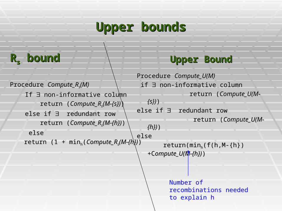
Upper boundsUpper bounds

RRss bound bound

Procedure Procedure Compute_RCompute_Rss(M)(M)

If If non-informative column non-informative column

return (return (Compute_RCompute_Rss(M-{s})(M-{s})))

else if else if redundant row redundant row

return (return (Compute_RCompute_Rss(M-{h})(M-{h})))

else else

return (1 + minreturn (1 + minhh((Compute_RCompute_Rss(M-{h})(M-{h})))

Upper BoundUpper Bound

Procedure Procedure Compute_U(M)Compute_U(M)

if if non-informative column non-informative column

return (return (Compute_U(M-{s})Compute_U(M-{s})))

else if else if redundant row redundant row

return (return (Compute_U(M-{h})Compute_U(M-{h})))

else else

return(minreturn(minhh(f(h,M-{h})(f(h,M-{h})+C+Compute_U(M-{h})ompute_U(M-{h})))

Number of recombinations needed to explain h

Many approaches to estimating Many approaches to estimating

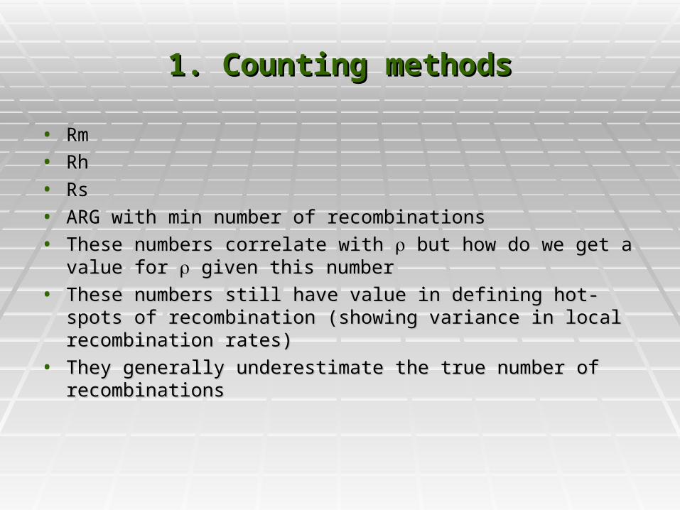
1. Counting methods1. Counting methods

• RmRm• RhRh• RsRs• ARG with min number of recombinationsARG with min number of recombinations• These numbers correlate with These numbers correlate with but how do we get a value but how do we get a value

for for given this number given this number• These numbers still have value in defining hot-spots of These numbers still have value in defining hot-spots of

recombination (showing variance in local recombination recombination (showing variance in local recombination rates)rates)

• They generally underestimate the true number of They generally underestimate the true number of recombinationsrecombinations

2. Model based approaches2. Model based approaches

Full likelihood approachesFull likelihood approaches

Approximate likelihood approachesApproximate likelihood approaches

Fearnhead, Donnelly

Approximate Likelihood Approximate Likelihood approachesapproaches

Two locus samplingTwo locus sampling 4 gamete violation implies recombination.4 gamete violation implies recombination. GeneralizationGeneralization

• Define vector Define vector nn = {n = {n0000, n, n01 01 , n, n1010,, nn1111}} for a pair of locifor a pair of loci

• The distribution of The distribution of n n depends upon depends upon , , • Can we compute Pr(Can we compute Pr(nn| | , , )? Then, we can iterate to get )? Then, we can iterate to get

the Max likelihood estimator for the Max likelihood estimator for ..

Two locus methodTwo locus method

• Generate MANY random ARGs with n= nGenerate MANY random ARGs with n= n0000+ n+ n0101+ + nn1010+ n+ n11 11 leaves.leaves.

• For each ARG, generate the two trees For each ARG, generate the two trees corresponding to the two locicorresponding to the two loci

• Drop 2 mutations at random, to get a value for Drop 2 mutations at random, to get a value for nn• How can you make this more efficient?How can you make this more efficient?• Given an ARG (topology), we know the edge pairs Given an ARG (topology), we know the edge pairs

that would generate desired that would generate desired nn..

•

Two locus estimationTwo locus estimation

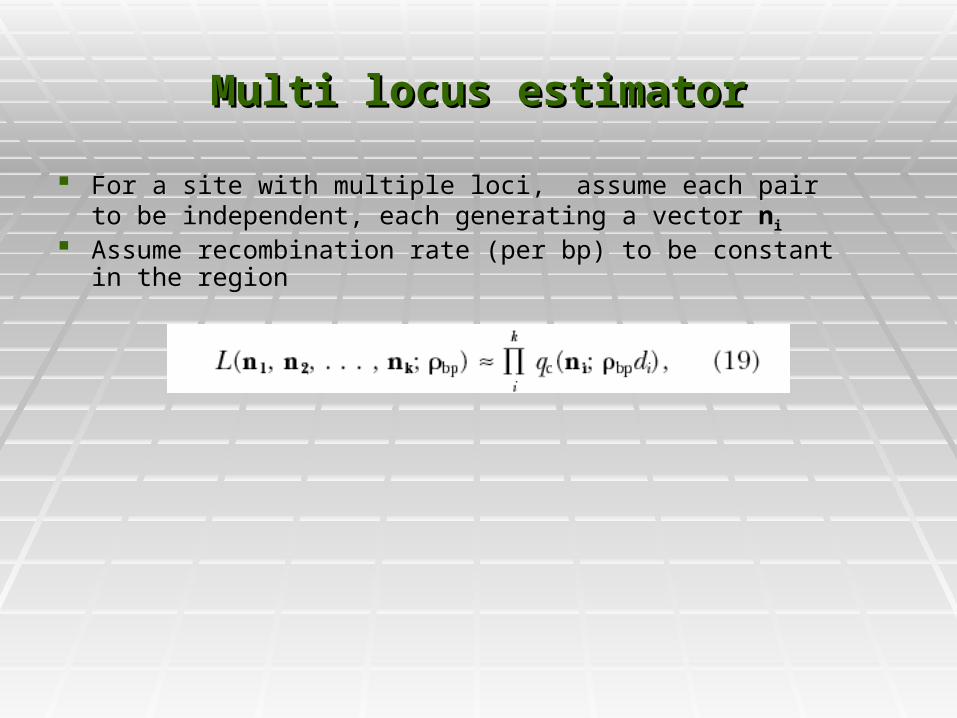
Multi locus estimatorMulti locus estimator

For a site with multiple loci, assume each pair to be For a site with multiple loci, assume each pair to be independent, each generating a vector independent, each generating a vector nnii

Assume recombination rate (per bp) to be constant in Assume recombination rate (per bp) to be constant in the regionthe region

Performance of the 2 locus Performance of the 2 locus estimatorestimator

The composite likelihood estimator performs ‘well’ in The composite likelihood estimator performs ‘well’ in practice.practice.

Note that the values of Note that the values of can be pre-computed making this can be pre-computed making this a fast method. a fast method.

Note that this plot does not describe the varianceNote that this plot does not describe the variance

Performancs: 90/10 percentilePerformancs: 90/10 percentile

Research: 2 locus versus other Research: 2 locus versus other statisticsstatistics

• Q1: Can we use some of the counting based methods as Q1: Can we use some of the counting based methods as summary statistic?summary statistic?

• It is better than composite likelihood in thatIt is better than composite likelihood in that• It does not assume independence between loci.It does not assume independence between loci.• There is a direct linear relationship (expected number of There is a direct linear relationship (expected number of

recombination events is recombination events is log n) log n)• Variation might be better.Variation might be better.

• Can we compute Pr(RCan we compute Pr(Rhh| | , , ) efficiently? In a sense, it does ) efficiently? In a sense, it does not matter, because we can pre-compute the numbers. not matter, because we can pre-compute the numbers.

• Incorporate distance constraints in computing these Incorporate distance constraints in computing these summary statistics. It is reasonable to assume that the rate summary statistics. It is reasonable to assume that the rate is constant per bp within a window.is constant per bp within a window.

Research ProblemResearch Problem

Recombination hot-spots are NOT correlated Recombination hot-spots are NOT correlated between humans and Chimps.between humans and Chimps. 99% sequence identity99% sequence identity Virtually no overlap between hot-spots (generated using Virtually no overlap between hot-spots (generated using

pop. Genetics). pop. Genetics). What can cause this?What can cause this?

MethodMethod Europeans/Africans share hot-spotsEuropeans/Africans share hot-spots Concordance with sperm typingConcordance with sperm typing

Population sub-structure? Not (as shown by structure)Population sub-structure? Not (as shown by structure) Genomic factorsGenomic factors

Genomic factorsGenomic factors

Recombination is elevated in GC rich regionsRecombination is elevated in GC rich regions Epigenetic factors (such as acetylation, Epigenetic factors (such as acetylation,

methylation) that affect chromatin structure methylation) that affect chromatin structure might be key.might be key.

Yeast is a useful model for studying Yeast is a useful model for studying recombinationrecombination

In yeast, recombination hotspots can be In yeast, recombination hotspots can be eliminated by insertion of transposable elements!eliminated by insertion of transposable elements!

Can differential insertion of Alus explain the Can differential insertion of Alus explain the differences between chimps/humans?differences between chimps/humans?

Haplotype PhasingHaplotype Phasing

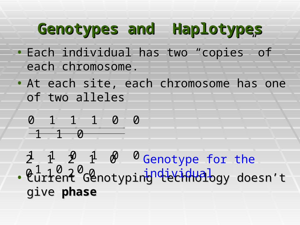
Genotypes and HaplotypesGenotypes and Haplotypes

• Each individual has two “copies” of each Each individual has two “copies” of each chromosome. chromosome.

• At each site, each chromosome has one of At each site, each chromosome has one of two allelestwo alleles

• Current Genotyping technology doesn’t give Current Genotyping technology doesn’t give phasephase

0 1 1 1 0 0 1 1 0

1 1 0 1 0 0 1 0 0

2 1 2 1 0 0 1 2 0 Genotype for the individual

Why is haplotype phasing important ?Why is haplotype phasing important ?

Haplotype PhasingHaplotype Phasing

Haplotype Phasing is the resolution of a Haplotype Phasing is the resolution of a genotype into the two haplotypes.genotype into the two haplotypes.

Haplotypes increase the power of an Haplotypes increase the power of an association between marker loci and association between marker loci and phenotypic traitsphenotypic traits

Current approaches to HaplotypingCurrent approaches to Haplotyping Via technological innovations (expensive)Via technological innovations (expensive) Statistical Methods (ML, Phase,PL)Statistical Methods (ML, Phase,PL)

This lecture, we will consider a combinatorial This lecture, we will consider a combinatorial approach to the phasing problemapproach to the phasing problem Efficient, provable quality of solutionEfficient, provable quality of solution Not completely generalizable (as yet)Not completely generalizable (as yet)

The Perfect Phylogeny ModelThe Perfect Phylogeny Model We assume that the We assume that the

evolution of extant evolution of extant haplotypes can be haplotypes can be displayed on a rooted, displayed on a rooted, directed tree, with the all-0 directed tree, with the all-0 haplotype at the root, haplotype at the root, where each site changes where each site changes from 0 to 1 on exactly one from 0 to 1 on exactly one edge, and each extant edge, and each extant haplotype is created by haplotype is created by accumulating the changes accumulating the changes on a path from the root to a on a path from the root to a leaf, where that haplotype leaf, where that haplotype is displayed. is displayed.

In other words, the extant In other words, the extant haplotypes evolved along a haplotypes evolved along a perfect phylogenyperfect phylogeny with all-0 with all-0 root.root.

00000

1

2

4

3

510100

1000001011

00010

01010

12345

Extant Haplotypes

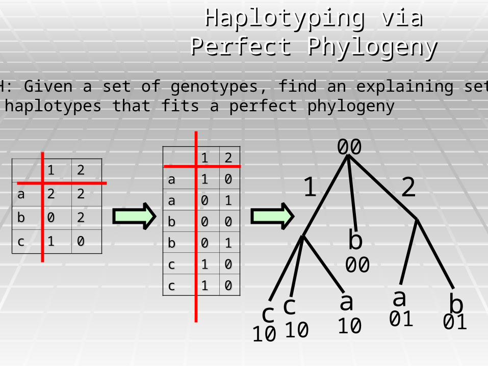
PPH: Given a set of genotypes, find an explaining set of haplotypes that fits a perfect phylogeny

11 22

aa 22 22

bb 00 22

cc 11 00

11 22

aa 11 00

aa 00 11

bb 00 00

bb 00 11

cc 11 00

cc 11 00

1

c c a a

b

b

2

10 10 10 01 01

00

00

Haplotyping via Perfect Haplotyping via Perfect PhylogenyPhylogeny

11 22

aa 22 22

bb 00 22

cc 11 00

11 22

aa 11 11

aa 00 00

bb 00 00

bb 00 11

cc 11 00

cc 11 00

No treepossiblefor thisexplanation

The Alternative ExplanationThe Alternative Explanation

Arrange the haplotypes in a matrix, two Arrange the haplotypes in a matrix, two haplotypes for each individual. haplotypes for each individual.

Then (with Then (with nono duplicate columns), the duplicate columns), the haplotypes fit a haplotypes fit a unique unique perfect phylogeny if perfect phylogeny if and only if no two columns contain all four and only if no two columns contain all four pairs (Buneman): pairs (Buneman):

0,0 and 0,1 and 1,0 and 1,10,0 and 0,1 and 1,0 and 1,1

The 4 Gamete Test for Perfect The 4 Gamete Test for Perfect PhylogenyPhylogeny

00

01 11

10

The Alternative Explanation

11 22

aa 22 22

bb 00 22

cc 11 00

11 22

aa 11 11

aa 00 00

bb 00 00

bb 00 11

cc 11 00

cc 11 00

No treepossiblefor thisexplanation

11 22

aa 22 22

bb 00 22

cc 11 00

11 22

aa 11 00

aa 00 11

bb 00 00

bb 00 11

cc 11 00

cc 11 00

1

c c a a

b

b

2

0 0

0 1 0 1

0 0

The Tree Explanation Again

The Combinatorial ProblemThe Combinatorial Problem

Input: A ternary matrix (0,1,2) M with N rowsInput: A ternary matrix (0,1,2) M with N rows Output: A binary matrix M’ created from M by Output: A binary matrix M’ created from M by

replacing each 2 in M with a 0 and 1, such that M’ replacing each 2 in M with a 0 and 1, such that M’ passes the 4 gamete testpasses the 4 gamete test

Gusfield (Recomb2002) proposed a solution Gusfield (Recomb2002) proposed a solution which used a reduction to Matroids. which used a reduction to Matroids.

We present a (slightly inefficient) solution using We present a (slightly inefficient) solution using elementary techniqueselementary techniques

Independently by (Eskin, Halperin, Karp’02)Independently by (Eskin, Halperin, Karp’02)

Initial Observations Initial Observations

Forced Expansions:Forced Expansions: EX 1: If two columns(sites) of M contain the following EX 1: If two columns(sites) of M contain the following

rowsrows 2 0 2 0 0 20 2

Then M’ will contain a row with 1 0 and a row with 0 1 Then M’ will contain a row with 1 0 and a row with 0 1 in those columns.in those columns.

EX 2: Similarly, if two columns of M contain the rowsEX 2: Similarly, if two columns of M contain the rows 2 1 2 1 2 0 2 0 Then M’ will contain rows with 1 1 and 0 0 in those Then M’ will contain rows with 1 1 and 0 0 in those

columnscolumns

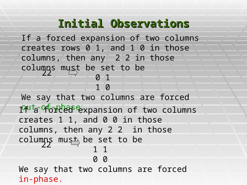
If a forced expansion of two columns creates rows 0 1, and 1 0 in those columns, then any 2 2 in those columns must be set to be

0 11 0

We say that two columns are forced out-of-phase.

If a forced expansion of two columns creates 1 1, and 0 0 in those columns, then any 2 2 in those columns must be set to be

1 10 0

We say that two columns are forced in-phase.

Initial ObservationsInitial Observations

22

22

Immediate FailureImmediate Failure

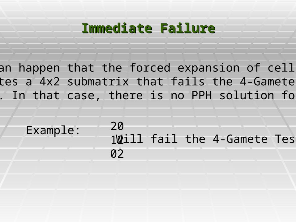
It can happen that the forced expansion of cellscreates a 4x2 submatrix that fails the 4-GameteTest. In that case, there is no PPH solution forM.

Example: 20 1202

Will fail the 4-Gamete Test

An O(ns^2)-time AlgorithmAn O(ns^2)-time Algorithm

Find all the forced phase relationships by Find all the forced phase relationships by considering columns in pairs.considering columns in pairs.

Find all the inferred, invariant, phase Find all the inferred, invariant, phase relationships.relationships.

Find a set of column pairs whose phase Find a set of column pairs whose phase relationship can be arbitrarily set, so that all relationship can be arbitrarily set, so that all the remaining phase relationships can be the remaining phase relationships can be inferred.inferred.

Result: An implicit representation of all Result: An implicit representation of all solutions to the PPH problem.solutions to the PPH problem.

11 22 22 22 00 00 00

22 00 22 00 00 00 22

11 22 22 22 00 22 00

11 22 22 00 22 00 00

22 22 00 00 00 22 00

00 00 00 00 00 00 00

A

B

C

D

E

F

1 2 3 4 5 6 7

A Running ExampleA Running Example

1

• Each node represents a column in M, and each edge indicates that the pair of columns has a row with 2’s in both columns.

•The algorithm builds this graph, and then checks whether any pair of nodes is forced in or out of phase.

4

7

25

3

6

1

Companion Graph G_cCompanion Graph G_c

11 22 22 22 00 00 00

22 00 22 00 00 00 22

11 22 22 22 00 22 00

11 22 22 00 22 00 00

22 22 00 00 00 22 00

00 00 00 00 00 00 00

A

B

C

D

E

F

1 2 3 4 5 6 7

1

7

25

34

6

•Each Red edge indicates that the columns are forced in-phase.

•Each Blue edge indicates that the columns are forced out-of-phase.

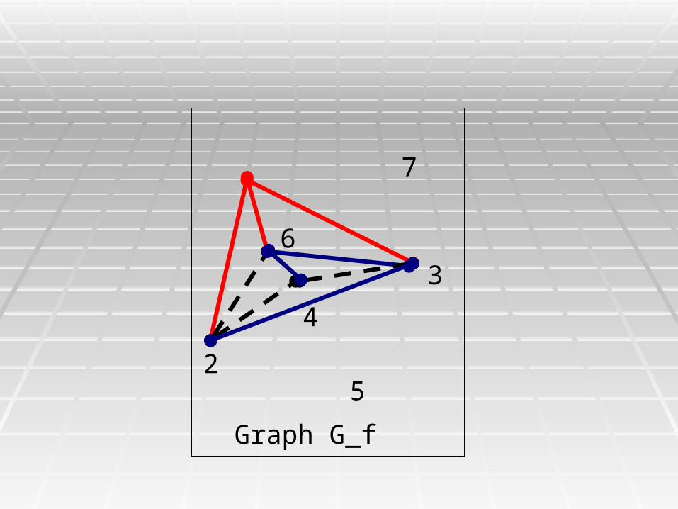
Let G_f be the sub-graph of G_cdefined by the red and blueedges.

Phasing Edges in G_cPhasing Edges in G_c

1

7

2

5

34

6

.

Connected Components in G_fConnected Components in G_f

Graph G_f has three Graph G_f has three connected componentsconnected components

Phase-parity LemmaPhase-parity Lemma

That’s nice, but how do we assign the colors?

Lemma 1: There is a solution to the PPH Lemma 1: There is a solution to the PPH problem for M if and only if there is a coloring problem for M if and only if there is a coloring of the black edges of G_c with the following of the black edges of G_c with the following property:property:

For any triangle in G_c containing at least one For any triangle in G_c containing at least one black edge, the coloring makes either 0 or 2 of black edge, the coloring makes either 0 or 2 of the edgesthe edges

blue (i.e., out of phase)blue (i.e., out of phase)

1 A Weak Triangulation RuleA Weak Triangulation Rule

Theorem 1: If there are any Theorem 1: If there are any black edges whose ends are in black edges whose ends are in the same connected the same connected component of G_f, at least one component of G_f, at least one edge is in a triangle where the edge is in a triangle where the other edges are not blackother edges are not black

In every PPH solution, it must In every PPH solution, it must be colored so that the triangle be colored so that the triangle has an even number of has an even number of Blue Blue (out of Phase) (out of Phase) edges.edges.

This an “inferred” coloringThis an “inferred” coloring..

3

Graph G_f

7

25

4

6

3

Graph G_f

7

25

4

6

3

Graph G_f

7

25

4

6

3

Graph G_f

7

25

4

6

3

Graph G_f

7

25

4

6

CorollaryCorollary

Inside any connected component of G_f, ALL the phase Inside any connected component of G_f, ALL the phase relationships on edges (columns of M) are uniquely relationships on edges (columns of M) are uniquely determined, either as forced relationships based on determined, either as forced relationships based on pair-wise column comparisons, or by triangle-based pair-wise column comparisons, or by triangle-based inferred colorings.inferred colorings.

Hence, the phase relationships of all the columns in a Hence, the phase relationships of all the columns in a connected component of G_f are INVARIANT over all the connected component of G_f are INVARIANT over all the solutions to the PPH problem.solutions to the PPH problem.

The black edges in G_f can be ordered so that the The black edges in G_f can be ordered so that the inferred colorings can be done in linear time. inferred colorings can be done in linear time. Modification of DFSModification of DFS. .

Phase Parity Lemma: ProofPhase Parity Lemma: Proof

22 XX

YY 22

22 22

If X ≠ 2, and Y ≠ 2, Then the two columns are forced

Phase Parity Lemma: proofPhase Parity Lemma: proof

22 22 yy

xx 22 22

22 zz 22

A B C Lemma: If a triangle contains a Lemma: If a triangle contains a black edge, then a PPH solution black edge, then a PPH solution exists only if there are 0 or 2 blue exists only if there are 0 or 2 blue edges in the final coloring.edges in the final coloring.

Proof: Proof: No black edge unless x==2, or No black edge unless x==2, or

y==2 or z==2 (previous lemma)y==2 or z==2 (previous lemma) If there is a row with all 2s, then If there is a row with all 2s, then

there must be an even number of there must be an even number of blue edgesblue edges

AC

B

Proof of Weak Triangulation Proof of Weak Triangulation TheoremTheorem

Arbitrary chordless Arbitrary chordless cycles are possible in the cycles are possible in the graph, with forced edges.graph, with forced edges. See example. The See example. The

pattern 0,2; 2,0; and 2,2 pattern 0,2; 2,0; and 2,2 implies a blue (out of implies a blue (out of phase) edgephase) edge

A single unforced edge A single unforced edge changes the picturechanges the picture

22 22 00 00 00

00 22 22 00 00

00 00 22 22 00

00 00 00 22 22

22 00 00 00 22

A B C D E

E

D

A

B

C

Proof of Weak Triangulation TheoremProof of Weak Triangulation Theorem

Let (J,J’) be a black edge Let (J,J’) be a black edge connecting a ‘long’ path connecting a ‘long’ path J,K,…K’,J’ of forced edgesJ,K,…K’,J’ of forced edges

In the Matrix, x ≠ 2, In the Matrix, x ≠ 2, otherwise there is a otherwise there is a chord. Likewise y≠2chord. Likewise y≠2

By previous lemma, (J,J’) By previous lemma, (J,J’) is forcedis forced

22 22 xx

yy 22 22

22 22

K J J’ K’

J J’

K K’

Finishing the SolutionFinishing the Solution

Problem: A connected component C of G may Problem: A connected component C of G may contain several connected components of G_f, so contain several connected components of G_f, so any edge crossing two components of G_f will still any edge crossing two components of G_f will still be black. How should they be colored?be black. How should they be colored?

1

4

6

7

25

3

How should we How should we color the color the remaining black remaining black edges in a edges in a connected connected component C of component C of G_c?G_c?

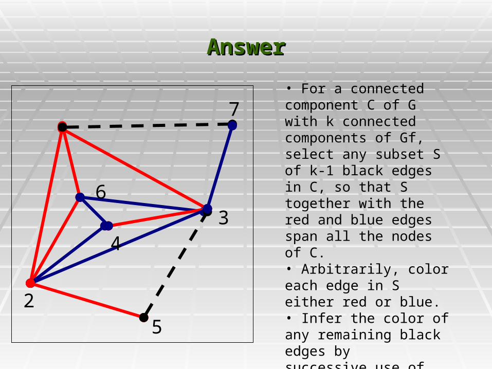
AnswerAnswer

• For a connected component C of G with k connected components of Gf, select any subset S of k-1 black edges in C, so that S together with the red and blue edges span all the nodes of C.• Arbitrarily, color each edge in S either red or blue.• Infer the color of any remaining black edges by successive use of the triangle rule.

7

25

34

6

7

25

34

6

Theorem 2Theorem 2

Any selected S works (allows the triangle rule Any selected S works (allows the triangle rule to work) and any coloring of the edges in S to work) and any coloring of the edges in S determines the colors of any remaining black determines the colors of any remaining black edges.edges.

Different colorings of S determine different Different colorings of S determine different colorings of the remaining black edges.colorings of the remaining black edges.

Each different coloring of S determines a Each different coloring of S determines a different solution to the PPH problem.different solution to the PPH problem.

All PPH solutions can be obtained in this way, All PPH solutions can be obtained in this way, i.e. using just one selected S set, but coloring i.e. using just one selected S set, but coloring it in all 2^(k-1) ways.it in all 2^(k-1) ways.

CorollaryCorollary

In a single connected component C of G with k In a single connected component C of G with k connected components in Gf, there are exactly 2^(k-1) connected components in Gf, there are exactly 2^(k-1) different solutions to the PPH problem in the columns of different solutions to the PPH problem in the columns of M represented by C.M represented by C.

If G_c has r connected components and t connected If G_c has r connected components and t connected components of G_f, then there are exactly 2^(t-r) components of G_f, then there are exactly 2^(t-r) solutions to the PPH problem.solutions to the PPH problem.

There is one unique PPH solution if and only if each There is one unique PPH solution if and only if each connected component in G is a connected component in connected component in G is a connected component in G_f.G_f.

ConclusionConclusion

In the special case of blocks with no recombination, and no In the special case of blocks with no recombination, and no recurrent mutations, the haplotypes satisfy a perfect recurrent mutations, the haplotypes satisfy a perfect phylogenyphylogeny

Given a set of genotypes, there is an efficient (O(ns^2)) Given a set of genotypes, there is an efficient (O(ns^2)) algorithm for representing all possible haplotype solutions that algorithm for representing all possible haplotype solutions that satisfy a prefect phylogenysatisfy a prefect phylogeny

Efficiency:Efficiency: Input is size O(ns), Input is size O(ns), All operations except building the graph are O(ns+s^2)All operations except building the graph are O(ns+s^2) Valid PPH only if s = O(n). Is O(ns) possible?Valid PPH only if s = O(n). Is O(ns) possible? Current best solution is O(ns+n^(1-e) s^2) using Matrix Current best solution is O(ns+n^(1-e) s^2) using Matrix

Multiplication ideaMultiplication idea Future work involves combining this with some heuristics to Future work involves combining this with some heuristics to

deal with general cases (lo recombination/hi recombination)deal with general cases (lo recombination/hi recombination)

Simulated DataSimulated Data

Coalescent model (Hudson)Coalescent model (Hudson) No RecombinationNo Recombination

400 chromosomes, 100 sites400 chromosomes, 100 sites Infinite sitesInfinite sites

RecombinationRecombination 100 chromosomes100 chromosomes Infinite sitesInfinite sites R=4.0 2501 R=4.0 2501

Pr(Recombination) = 4*10^(-9) between adjacent basesPr(Recombination) = 4*10^(-9) between adjacent bases

Error MeasurementError Measurement

Discrepancy = 1 Discrepancy = 1 (Num Haplotypes incorrectly (Num Haplotypes incorrectly predicted)predicted)

Switch Error = 2 Switch Error = 2

0010101010

0000011111

0101000101

0101010101

02222

22222

No RecombinationNo Recombination

Haplotype discrepancy

0

5

10

15

20

25

30

35

40

45

50

0 0.2 0.4 0.6 0.8 1 1.2 1.4

% Error

# results

Series1

No RecombinationNo Recombination

Switch Error

0

5

10

15

20

25

30

35

40

0 0.1 0.15 0.2 0.25 0.3 0.35 0.4

% Error

% Results

Series1

Choosing between solutionsChoosing between solutions

-1600

-1550

-1500

-1450

-1400

-1350

-1300

-12501 9 17 25 33 41 49 57 65 73 81 89 97 105 113 121

log(likelihood)

0

1

2

3

4

5

6

discrepancy

Series2Series1

Choosing between solutionsChoosing between solutions

Entropy vs Discrepancy

2.69

2.7

2.71

2.72

2.73

2.74

2.75

1 8 15 22 29 36 43 50 57 64 71 78 85 92 99 106 113 120 127

Equivalent Solutions

Entropy

0

1

2

3

4

5

6

Discrepancy

Series2Series1

Choosing between solutionsChoosing between solutions

Parsimony vs. Discrepancy

31

31.5

32

32.5

33

33.5

34

34.5

1 8 15 22 29 36 43 50 57 64 71 78 85 92 99 106 113 120 127

Equivalent Solutions

# Haplotypes

0

1

2

3

4

5

6

Discrepancy

Series2Series1

ConclusionConclusion

Extremely low error rates (< 1% discrepancy) Extremely low error rates (< 1% discrepancy) if no recombinationif no recombination

Randomly choosing between equivalent Randomly choosing between equivalent solutions is sufficientsolutions is sufficient

Other measures (Parsimony, Likelihood, Other measures (Parsimony, Likelihood, Entropy) do not improve the quality of solutionEntropy) do not improve the quality of solution

Haplotype Discrepancy (R=4.0)

0

2

4

6

8

10

12

14

1 3 5 7 9 11 13 15 17 19 21 23 25 27 29

% Error

% predictions

Series1

With RecombinationWith Recombination