LA-UR-Approved for public release;distribution is unlimited.

Title:

Author(s):

Details::

Form 836 (8/00)

Los Alamos National Laboratory, an affirmative action/equal opportunity employer, is operated by the University of California for the U.S.Department of Energy under contract W-7405-ENG-36. By acceptance of this article, the publisher recognizes that the U.S. Governmentretains a nonexclusive, royalty-free license to publish or reproduce the published form of this contribution, or to allow others to do so, for U.S.Government purposes. Los Alamos National Laboratory requests that the publisher identify this article as work performed under theauspices of the U.S. Department of Energy. Los Alamos National Laboratory strongly supports academic freedom and a researcher’s right topublish; as an institution, however, the Laboratory does not endorse the viewpoint of a publication or guarantee its technical correctness.

04-2131

CONTOUR-METHOD DETERMINATION OF PARENT-PART RESIDUAL STRESSES USING A PARTIALLY RELAXED FSW TEST SPECIMEN

Michael B. Prime (ESA-WR)Robert J. Sebring (MST-7)John M. Edwards (MST-7)John A. Baumann (Boeing St. Louis)Richard J. Lederich (Boeing St. Louis)

Proceedings of the 2004 SEM X International Congress & Exposition on Experimental and Applied Mechanics,June 7-10, 2004, Costa Mesa, California USApaper number 144 (CD-ROM proceedings)

Contour-Method Determination of Parent-Part Residual Stresses Using a Partially Relaxed FSW Test Specimen

Michael B. Prime, Technical Staff Member (prime@lanl.gov) Robert J. Sebring, Technical Staff Member

John M. Edwards, Technician Los Alamos National Laboratory, Los Alamos, NM 87545

John A. Baumann, Associate Technical Fellow

Richard J. Lederich, Associate Technical Fellow The Boeing Company, St. Louis, MO 63166-0516

ABSTRACT The residual stresses in a dissimilar aluminum-alloy friction stir weld were determined using the contour method on a small test specimen removed from the parent part. A butt joint in 25.4-mm thick plates of 7050-T7451 and 2024-T351 was produced by friction stir welding (FSW). A 54-mm long and 162-mm wide specimen was removed from the parent plate which was 457-mm long in the welding direction and 305-mm wide. A cross-sectional map of residual stresses at the mid-length the test specimen was measured using the contour method: 1) the specimen was carefully cut in two using wire electric discharge machining; 2) the contour of the cut surfaces were measured by laser scanning; and 3) the residual stresses were determined from the measured contours using a 3-D elastic finite element (FE) model. Because of the small size of the removed specimen, the pre-relaxation stresses were assumed to have changed and were estimated using a simple, iterative procedure with the previous FE mesh. This FE analysis simulated the relaxation of stresses from removing the test specimen in order to determine the parent-part stresses that would relax into the stresses measured in the test specimen. Because an iterative procedure was used, no assumptions (such as some functional form) had to be made about the un-relaxed stresses. The iteration converged quickly, and the peak stresses had indeed relaxed by about 25% from 43 MPa to 32 MPa. The procedure developed here could have many applications because of the convenience of measuring small test specimens.

Introduction Friction Stir Welding is a revolutionary joining process which has seen remarkable growth in research, development and application in recent years. Conventional structural components for aircraft - beams for floors, spars, with tailored characteristics to meet durability and damage tolerance requirements, and so on - are normally accomplished through built-up structure using discrete components of different alloys. To reduce the costs associated with conventional alignment and assembly steps of built-up structure, ever more assembled components are being converted to unitized structure via such processes as casting or machining from forged performs or thick plate stock. Friction Stir Welding offers additional avenues to unitization of structural components. Lap and butt joining of thin sheet materials provides an alternative to conventional joining/fastening. Another pathway to structural components is the fabrication of “tailored blanks,” using FSW to join shaped blocks of plate or forgings, from which unitized parts may be machined. Both of these approaches are in various stages of development and production. FSW has sufficiently matured such that direct joining of 1-inch thick plates of 2XXX or 7XXX alloys is currently within the state of the art, creating starting stock with distributed property characteristics [1]. Static strengths in such joints typically exceed 80% of the parent strength of the weaker alloy. Investigations of durability characteristics are underway. A significant potential contributor to the durability behavior of FSW joints and surrounding material, however, will be the magnitude and distribution of residual stress imparted by the FSW process. Measuring the residual stresses and understanding how the precise processing conditions impact the level and distribution of residual stresses are key activities in tailoring the process to achieve acceptably performing joints. Small test specimens are often removed from a parent part to measure residual stresses, even though the parent-part residual stresses are usually what is desired. Experimental considerations often limit the specimen size in which residual stresses can be measured. For example, most x-ray measurement goniometers can only accommodate moderately sized specimens. However, removing a small test specimen will change the stress state in a part because of the elastic relaxation of residual stresses. Because residual stresses satisfy force and moment equilibrium over a cross-section and therefore have equivalent force and moment of zero, St. Venant’s principle dictates that the residual stresses are unchanged if they are measured

sufficiently far away from the cuts used to remove the test specimen. Unfortunately, it is often not possible to use a large enough test specimen so that the stresses are unchanged at the location of measurement. In this paper, we demonstrate that the contour method for measuring residual stress provides enough information to estimate the parent-part residual stresses from measurement of partially relaxed stresses in a removed test specimen. When the test specimen is removed by sectioning the parent part in only one direction, the estimation is straightforward and unique.

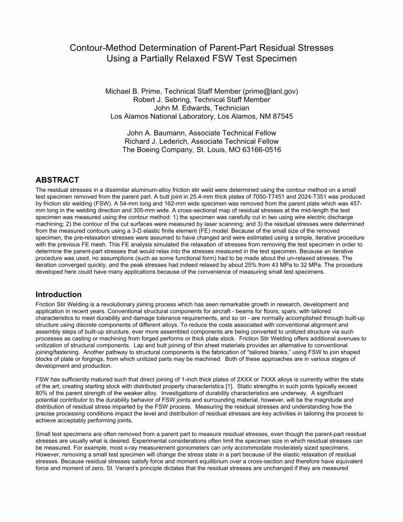
Specimen Plates of 25.4mm thickness of 7050-T7451 and 2024-T351 were procured from a commercial vender. The Edison Welding Institute (EWI) in Columbus, OH performed friction stir butt welding to produce a 305mm x 457mm plate from two 153mm x 457mm plates. A one-pass single sided joint was formed at a rate of 2 ipm. This particular weldment was fabricated by locating the 2024-T351 panel on the advancing side of the weld. X-ray radiography and metallographic cross sections verified that the joint was sound and free of voids and root surface disbands. After welding the panel was aged at 121°C for 24 hours to stabilize the weld nugget. A significant portion of the panel was consumed by microstructure and mechanical property characterization. The 54mm x 162mm sample was extracted initially for residual stress determinations using neutron diffraction.

Figure 1. The parent weld plate showing dimensions and location of test specimen that was removed from the center. The coordinate system origin is the center of the bottom face of the test specimen.

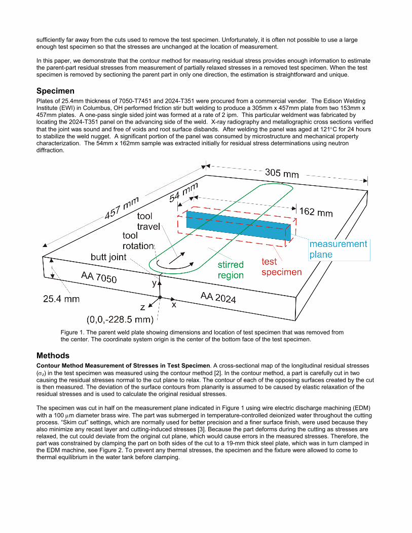
Methods Contour Method Measurement of Stresses in Test Specimen. A cross-sectional map of the longitudinal residual stresses (σz) in the test specimen was measured using the contour method [2]. In the contour method, a part is carefully cut in two causing the residual stresses normal to the cut plane to relax. The contour of each of the opposing surfaces created by the cut is then measured. The deviation of the surface contours from planarity is assumed to be caused by elastic relaxation of the residual stresses and is used to calculate the original residual stresses. The specimen was cut in half on the measurement plane indicated in Figure 1 using wire electric discharge machining (EDM) with a 100 µm diameter brass wire. The part was submerged in temperature-controlled deionized water throughout the cutting process. “Skim cut” settings, which are normally used for better precision and a finer surface finish, were used because they also minimize any recast layer and cutting-induced stresses [3]. Because the part deforms during the cutting as stresses are relaxed, the cut could deviate from the original cut plane, which would cause errors in the measured stresses. Therefore, the part was constrained by clamping the part on both sides of the cut to a 19-mm thick steel plate, which was in turn clamped in the EDM machine, see Figure 2. To prevent any thermal stresses, the specimen and the fixture were allowed to come to thermal equilibrium in the water tank before clamping.

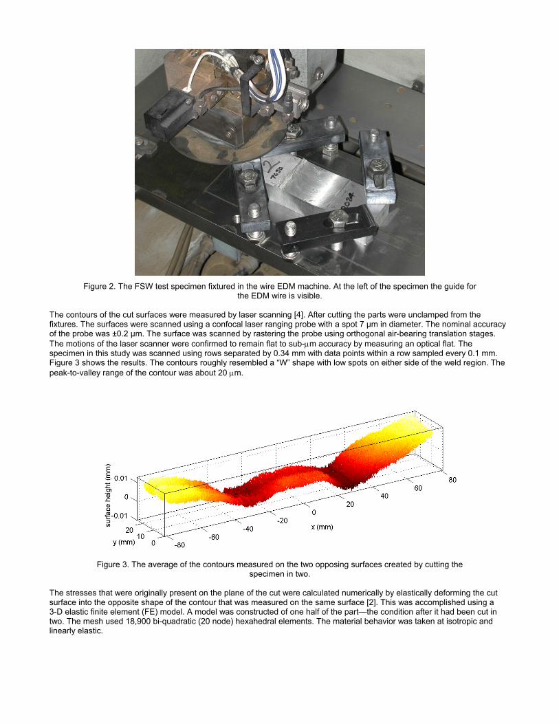
Figure 2. The FSW test specimen fixtured in the wire EDM machine. At the left of the specimen the guide for

the EDM wire is visible. The contours of the cut surfaces were measured by laser scanning [4]. After cutting the parts were unclamped from the fixtures. The surfaces were scanned using a confocal laser ranging probe with a spot 7 µm in diameter. The nominal accuracy of the probe was ±0.2 µm. The surface was scanned by rastering the probe using orthogonal air-bearing translation stages. The motions of the laser scanner were confirmed to remain flat to sub-µm accuracy by measuring an optical flat. The specimen in this study was scanned using rows separated by 0.34 mm with data points within a row sampled every 0.1 mm. Figure 3 shows the results. The contours roughly resembled a “W” shape with low spots on either side of the weld region. The peak-to-valley range of the contour was about 20 µm.

Figure 3. The average of the contours measured on the two opposing surfaces created by cutting the

specimen in two. The stresses that were originally present on the plane of the cut were calculated numerically by elastically deforming the cut surface into the opposite shape of the contour that was measured on the same surface [2]. This was accomplished using a 3-D elastic finite element (FE) model. A model was constructed of one half of the part—the condition after it had been cut in two. The mesh used 18,900 bi-quadratic (20 node) hexahedral elements. The material behavior was taken at isotropic and linearly elastic.

A single value of elastic modulus was used for all regions in the model. Typical values for the elastic modulus of 2024 aluminum are 73.1 GPa in tension and 74.5 GPa in compression, and for 7050 aluminum 70.6 GPa in tension and 72.7 GPa in compression [5]. The average, 72.7 GPa, of these values was used. The range in these values of ±3% from the average is no greater than other error sources in the measurement; therefore, the effort to more precisely account for spatial variations in elastic modulus is not warranted. Poisson’s ratio was taken as 0.33, which is the reported value for both 2024 and 7050. For the stress calculation, the opposite of the measured surface contour was applied as displacement boundary conditions on the surface corresponding to the cut. The steps outlined here to process discrete surface contour data, i.e., the point clouds, into a form suitable for calculating the stresses with the FE model are described in more detail elsewhere [4]. The point clouds from the two opposing surfaces created by a cut were aligned to each other, then interpolated onto a common, regular grid and then averaged point by point. (Averaging the two contours is crucial to minimize several error sources [2]). Next, the data were fit to a smooth surface using smoothing splines. The amount of smoothing was selected by minimizing the estimated uncertainty in the results. Finally, heights of the smoothed surface were evaluated at the coordinates of the nodes in the finite element model, the signs were reversed, and the results were written into the FE input file as displacement boundary conditions. Estimation of Parent-Part Stresses. The stress relaxation from removing the test specimen was assumed elastic. The stress magnitudes will be seen to be small, so stress relaxation away from the cut would not have any plasticity. The cutting process will cause some plastic deformation in local regions very near the cuts. However, the measurement plane is far enough from the cuts that the local plasticity will have no effect on the measurements. Since elasticity is assumed, the problem is path-independent and the actual order that the cuts are examined is irrelevant. Nonetheless, it is conceptually convenient to consider that we examine the cuts in reverse chronological order. Thus the relaxation caused by shortening the specimen from 457 mm long to 54 mm is considered to be the second step in the specimen removal and is examined first and in detail. Next, shortening the width from 305 mm to 162 mm is examined. In that case, a reasonable argument is made that the stress change was negligible.

Shortening length. The residual stresses prior to the two cuts to make the test specimen 54-mm long were estimated using reasonable assumptions and a straightforward calculation. First, it was assumed that before the test specimen was removed, the parent-plate stresses in the region of the test specimen did not vary in the longitudinal (welding) direction. Because of the steady state nature of the welding process, and because the test specimen was not close to the ends of the parent plate, that was a reasonable assumption. It was not necessary to assume that the stresses were uniform elsewhere because stresses outside of the region of the test specimen do not affect the relaxation when the test specimen is removed. Second, shear stresses normal to the longitudinal direction, i.e., τxz and τyz, were assumed to be negligible, which was consistent with the assumption of stress uniformity on the longitudinal direction. The problem was then an inverse problem to determine residual stresses in the parent plate that would relax into the residual stresses measured in the mid-length of the test specimen. An iterative solution to the problem allowed this to be calculated without making any a priori assumptions, such as assuming a functional form, about the stresses. Because the test specimen length was a little over twice the plate thickness, the stresses at the mid-length in the test specimen should not have relaxed grossly. Therefore, the stresses measured at mid-length in the test specimen made a reasonable starting point for an iterative solution. The amount that these stresses would relax when the specimen was removed was calculated. Comparing the relaxed stresses on the midlength to the measured stresses allowed a new estimate of the original stresses. The process was repeated until convergence as follows:

1. Based on initial guess for parent-part stress ( )ioσ for iteration i, calculate the relaxed stresses at the midlength of the test specimen ( )irσ . This calculation is detailed later. For the zeroth iteration, use the measured test-specimen stress as the guess: ( ) s

io σσ ==0 .

2. Use the difference between the actual relaxed stresses (measured in the specimen) and the calculated relaxed stresses to adjust the guess at the original stresses: ( ) ( ) ( )[ ]irs

io

io σσσσ −+=+1

3. When ( ) si

r σσ = within acceptable bounds, then ( )ioσ is the estimated original stress. Where

oσ = the Orignal stresses in the parent plate, uniform in the longtidunal direction sσ = Specimen: the stresses measured at the midlength in the test specimen rσ = Relaxed: the calculated relaxed stresses at the midlength in the test specimen

There are two methods to calculate the stress relaxation when the specimen is removed from the parent plate. Both use the same FE mesh that was previously used with the contour method measurements, which saves additional meshing effort. Using that mesh of half of the test specimen, the surface representing the midlength of the specimen was constrained in the longitudinal direction to enforce the symmetry inherent in the problem. The first method, which was used in this study, to

calculate the relaxation stresses is to apply the assumed original stresses as an initial stress throughout the model. The longitudinal stresses are thus initialized uniformly along the length of the model, and all other stress components are zeroed. The surface opposite the symmetry plane represents the cut that removed the test specimen, and is left unconstrained. Therefore, a static equilibrium FE analysis will enforce the stress-free free-surface condition there, allow the stresses to relax, and give the relaxed stresses throughout the test specimen. The second method is useful for FE codes that do not have an initial stress option. The stress relaxation can be calculated by applying the opposite of the initial stress as a distributed pressure load on the surface opposite the symmetry plane. The resulting stresses on the symmetry plane are then the change in those stresses, and the relaxed stresses are given by adding the change stresses to the initial stress. The initial stress was implemented using the ABAQUS user subroutine sigini.f. The σr or σs stresses at the nodes of the symmetry surface were taken from ABAQUS output of nodal stresses averaged from all elements sharing a node and then saved as text files. When the FE analysis for each iteration first called sigini.f, it read the appropriate files from previous runs and calculated the new σ0 initial stress as described in step 2 of the iteration procedure described above. For each subsequent call in a given analysis, sigini.f only had to return σ0 for the provided coordinates, which were the integration points of all elements on the model. Bilinear interpolation was used to determine the stresses at these points from the values at nodal coordinates. To make an approximately rectangular grid for simpler interpolation, the stresses were only used from the corner nodes on the cut surface, not the mid-side nodes. A test run verified that this interpolation scheme reproduced the desired stresses quite accurately. A sample sigini.f and other files are given in the appendix.

Shortening Width. No correction was made for the first operation in removing the test specimen: shortening the width from 305 mm to 162 mm, which would relax σx. After examining the results of the measurement of residual σz in the test specimen, it was concluded that the operation of shortening the width had negligible impact on the residual stresses measured near the weld, which was the quantity of interest. The residual stresses away from the weld were very low, on the order of ±20 MPa. Such stresses are exactly what is expected in rolled aluminum plate that is stress relieved by stretching [6]. Because residual stresses satisfy equilibrium over the cross section and the magnitudes are so low, St. Venant’s principle tells us that the effect in the nearest region of interest will be small. FE calculations verified that at the heat-affected region, 1.9 plate thicknesses away from these cuts, the effect on σx probably is less than 2% of the relaxed stresses, or less than 1MPa in this case The effect on σz, the quantity of interest, will be even less. A correction for such transverse cuts, if it were significant, would have required an additional contour method measurement to get the transverse (σx) stresses in the test specimen.

Results Figure 4 shows the contour-method measured residual stress measured in the test specimen. The stress magnitudes range from about -30 MPa to +32 MPa. These magnitudes are only about 0.044 % of the elastic modulus, which could make measurement sensitivity an issue for many measurement methods. Nonetheless, the surface contour was significant enough to measure easily, making the results reasonably precise with an estimated uncertainty of about ±5 MPa. The results agree quite well with neutron diffraction measurements on the same part [7], which will be reported in a future publication.

Figure 4. Residual longitudinal stresses measured in test specimen removed from friction stir welded plate. Figure 1 Shows the location of the measurement.

Figure 5 shows the residual stress estimate for pre-relaxation stresses in the parent plate. Comparing with Figure 4, the specimen removal caused the tensile stresses to relax by up to about 10 MPa in the test specimen, or about 25% the peak value of about 43 MPa. These stresses would generally be considered small when compared with the material yield strength of 220 MPa measured for this bi-alloy specimen. However, even these fairly low magnitude stresses can have a large effect on fatigue and fracture behavior [8].

Figure 5. Estimated longitudinal residual stress in parent plate before stresses were partially relaxed from removing test specimen.

Discussion Iterative Solution For Parent Part Stresses. The iterative solution for the residual stresses in the parent plate converges quickly. The convergence is evaluated by examining the difference between the estimated and actual relaxed stresses at the midplane: rs σσ − . This also equals the difference between successive estimates of the parent-plate stresses, which are the results being sought. Figure 6 shows that after only 5 iterations both the maximum and average difference are below 1 MPa.

Figure 6. Difference between the estimated and measured stresses at the midplane, showing convergence of estimate.

Figure 7 shows the estimated initial stresses at the mid-thickness, y = 12.7 mm, of the plate for the first eight iterations. Again, the estimate has converged quite well within about three iterations. The stresses have relaxed by up 10 MPa in the test specimen, or about 25% the peak value of about 40 MPa.

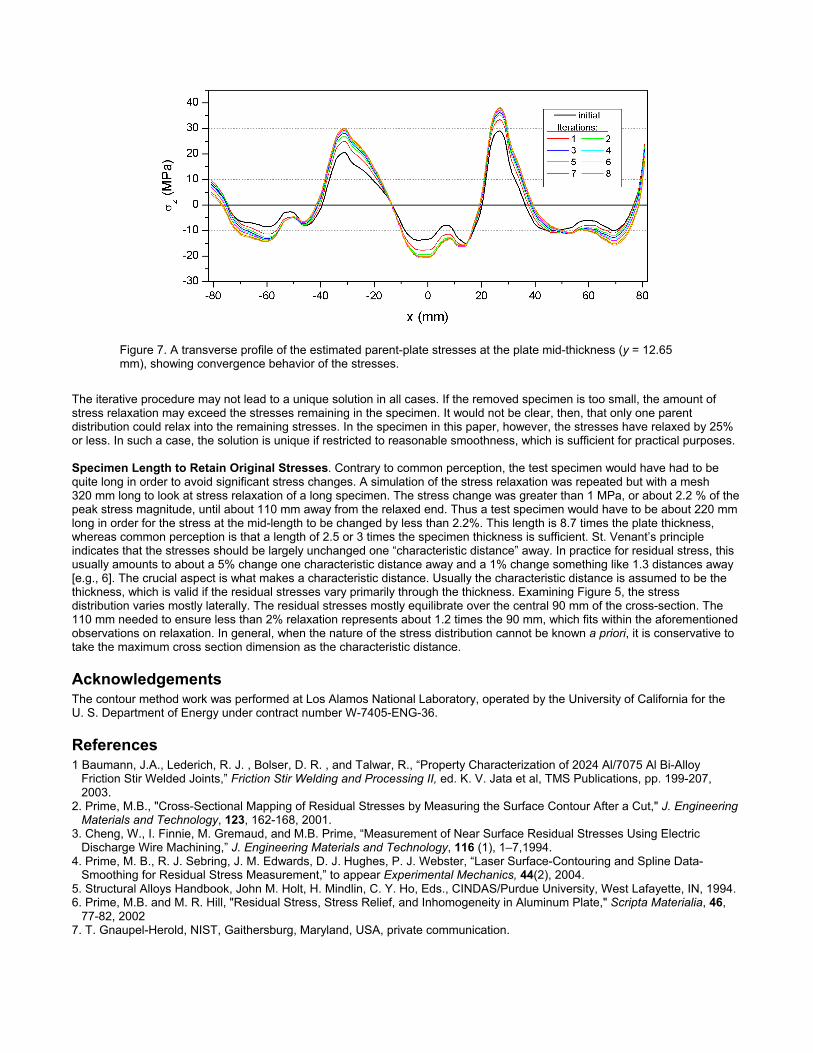
Figure 7. A transverse profile of the estimated parent-plate stresses at the plate mid-thickness (y = 12.65 mm), showing convergence behavior of the stresses.

The iterative procedure may not lead to a unique solution in all cases. If the removed specimen is too small, the amount of stress relaxation may exceed the stresses remaining in the specimen. It would not be clear, then, that only one parent distribution could relax into the remaining stresses. In the specimen in this paper, however, the stresses have relaxed by 25% or less. In such a case, the solution is unique if restricted to reasonable smoothness, which is sufficient for practical purposes. Specimen Length to Retain Original Stresses. Contrary to common perception, the test specimen would have had to be quite long in order to avoid significant stress changes. A simulation of the stress relaxation was repeated but with a mesh 320 mm long to look at stress relaxation of a long specimen. The stress change was greater than 1 MPa, or about 2.2 % of the peak stress magnitude, until about 110 mm away from the relaxed end. Thus a test specimen would have to be about 220 mm long in order for the stress at the mid-length to be changed by less than 2.2%. This length is 8.7 times the plate thickness, whereas common perception is that a length of 2.5 or 3 times the specimen thickness is sufficient. St. Venant’s principle indicates that the stresses should be largely unchanged one “characteristic distance” away. In practice for residual stress, this usually amounts to about a 5% change one characteristic distance away and a 1% change something like 1.3 distances away [e.g., 6]. The crucial aspect is what makes a characteristic distance. Usually the characteristic distance is assumed to be the thickness, which is valid if the residual stresses vary primarily through the thickness. Examining Figure 5, the stress distribution varies mostly laterally. The residual stresses mostly equilibrate over the central 90 mm of the cross-section. The 110 mm needed to ensure less than 2% relaxation represents about 1.2 times the 90 mm, which fits within the aforementioned observations on relaxation. In general, when the nature of the stress distribution cannot be known a priori, it is conservative to take the maximum cross section dimension as the characteristic distance.

Acknowledgements The contour method work was performed at Los Alamos National Laboratory, operated by the University of California for the U. S. Department of Energy under contract number W-7405-ENG-36.

References 1 Baumann, J.A., Lederich, R. J. , Bolser, D. R. , and Talwar, R., “Property Characterization of 2024 Al/7075 Al Bi-Alloy

Friction Stir Welded Joints,” Friction Stir Welding and Processing II, ed. K. V. Jata et al, TMS Publications, pp. 199-207, 2003.

2. Prime, M.B., "Cross-Sectional Mapping of Residual Stresses by Measuring the Surface Contour After a Cut," J. Engineering Materials and Technology, 123, 162-168, 2001.

3. Cheng, W., I. Finnie, M. Gremaud, and M.B. Prime, “Measurement of Near Surface Residual Stresses Using Electric Discharge Wire Machining,” J. Engineering Materials and Technology, 116 (1), 1–7,1994.

4. Prime, M. B., R. J. Sebring, J. M. Edwards, D. J. Hughes, P. J. Webster, “Laser Surface-Contouring and Spline Data-Smoothing for Residual Stress Measurement,” to appear Experimental Mechanics, 44(2), 2004.

5. Structural Alloys Handbook, John M. Holt, H. Mindlin, C. Y. Ho, Eds., CINDAS/Purdue University, West Lafayette, IN, 1994. 6. Prime, M.B. and M. R. Hill, "Residual Stress, Stress Relief, and Inhomogeneity in Aluminum Plate," Scripta Materialia, 46,

77-82, 2002 7. T. Gnaupel-Herold, NIST, Gaithersburg, Maryland, USA, private communication.

8. John, R, K. V. Jata, and K. Sadananda, “Residual Stress Effects on Near-Threshold Fatigue Crack Growth in Friction Stir Welds in Aerospace Alloys,” Int. J. of Fatigue, 25(9-11), 939-948, 2003.

Appendix Sample files for the finite element analysis are presented here to help others that may want to use this procedure. The sample files are presented in sufficient detail to allow understanding of the procedure. To conserve space some of the details are omitted, such as the node and element definitions. A. The ABAQUS input file used for all of the stress relaxation computations.

*HEADING Stress relaxation in friction stir weld test specimen ** ** Relax: apply initial stress and let relax to simulate parting out ** Import mesh: *INCLUDE,INPUT=/raid4/prime/contour/FSW/fswNBmesh.inp ** *SOLID SECTION, ELSET=ALUM, MATERIAL=ALUMAVG 1., ** *MATERIAL, NAME=ALUMAVG ** *ELASTIC, TYPE=ISO 72700., 0.33 ** *INITIAL CONDITIONS, TYPE=STRESS, USER ** *STEP Equilibrium step *STATIC ** *BOUNDARY, OP=NEW 1, 1,2, 0. 181, 2,, 0. CUT, 3,, 0. ** ** ‘CUT’ is a node set of all the nodes on the cut surface ** *OUTPUT,FIELD *ELEMENT OUTPUT S *NODE OUTPUT U ** *NODE PRINT, FREQ=0 *NODE FILE, FREQ=0 ** to get element stresses at nodes: *EL PRINT, POS=AVERAGED AT NODES, ELSET=END, FREQ=1 S11,S22,S33 ** *END STEP **

B. sigini.f: the initial stress user subroutine for one of the iterations:

subroutine sigini(sigma,coords,ntens,ncrds,noel,npt,layer, 1 kspt,lrebar,rebarn) c c !! because of "floor" function, needs f90 compile c see ABAQUS manual include 'ABA_PARAM.INC' c c For iterative solution to find initial FSW stresses in long plate c c 2: 2nd iteration (S-init)2=(S-init)1+(S-actual-relaxed)-(S-relaxed)0 c it02.dat it01.dat initial.dat relax01.dat data iFirst/0/ dimension sigma(ntens),coords(ncrds) c x and y are coordinates of corners of cross section

dimension x(4),y(4) data x,y / -80.75,-81.,80.65,81.,0.,25.3,25.35,-0.16/ character junk*60 common/kstress/stress(3989,3) iFirst=iFirst+1 c NEED TO READ FILE ONLY FIRST TIME ------------------------------------- if (iFirst .le. 1) then c read in header lines, must be 5 open(15,file="/raid4/prime/contour/FSW/iterate/initial.dat") open(16,file="/raid4/prime/contour/FSW/iterate/relax01.dat") open(17,file="/raid4/prime/contour/FSW/iterate/it01.dat") open(18,file="/scratch/prime/FSWrelax/it02.dat") c All of these files have 5 lines of text before data do 10 i=1,5 read(15,101)junk read(16,101)junk read(17,101)junk 10 continue c read in corner node values only. Skip mid-side nodes. do 20 i2=1,15 do 15 j=1,90 read(15,*) it1,(stress(91*(i2-1)+j,ii),ii=1,3) read(15,101)junk read(16,*) it1,t1,t2,t3 read(16,101)junk stress(91*(i2-1)+j,3)=stress(91*(i2-1)+j,3)-t3 15 continue read(15,*) it1,(stress(91*(i2-1)+j,ii),ii=1,3) read(16,*) it1,t1,t2,t3 stress(91*(i2-1)+j,3)=stress(91*(i2-1)+j,3)-t3 do 17 j2=1,91 read(15,101)junk read(16,101)junk 17 continue 20 continue c Now, since it01.dat is already on corner nodes, read it in and add it do 30 i3=1,1365 read(17,*) t1,t2,t3 stress(i3,3)=stress(i3,3)+t3 c write out results to file for use with next iteration: write(18,*)(stress(i3,ii),ii=1,3) 30 continue end if c -END READ FILE FIRST TIME --------------------------------------------- c Set initial stress for given location xx=coords(1) yy=coords(2) c Number of elements in rectangular grid: nx=90 ny=14 c find index of node to lower left of given (x,y) xmx=(yy-y(4))/(y(3)-y(4))*(x(3)-x(4))+x(4) xmn=(yy-y(1))/(y(2)-y(1))*(x(2)-x(1))+x(1) fx=(xx-xmn)/(xmx-xmn) ymx=(xx-x(2))/(x(3)-x(2))*(y(3)-y(2))+y(2) ymn=(xx-x(1))/(x(4)-x(1))*(y(4)-y(1))+y(1) fy=(yy-ymn)/(ymx-ymn) ix=floor(fx*nx)+1 iy=floor(fy*ny)

ii=91*iy+ix c Interpolate from nearest 4 grid points x1=stress(ii,1) y1=stress(ii,2) x4=stress(ii+1,1) y4=stress(ii+1,2) x2=stress(ii+91,1) y2=stress(ii+91,2) x3=stress(ii+92,1) y3=stress(ii+92,2) xmx=(yy-y4)/(y3-y4)*(x3-x4)+x4 xmn=(yy-y1)/(y2-y1)*(x2-x1)+x1 fx=(xx-xmn)/(xmx-xmn) ymx=(xx-x2)/(x3-x2)*(y3-y2)+y2 ymn=(xx-x1)/(x4-x1)*(y4-y1)+y1 fy=(yy-ymn)/(ymx-ymn) c Initalize longitudinal stress with interpolated value c All other stresses are zero c 3D els: S11,S22,S33,S12,S13,S23 sigma(3)=(1-fx)*(1-fy)*stress(ii,3)+fx*(1-fy)*stress(ii+1,3)+ & fx*fy*stress(ii+92,3)+(1-fx)*fy*stress(ii+91,3) sigma(1)=0 sigma(2)=0 sigma(4)=0 sigma(5)=0 sigma(6)=0 101 format(a) return end

C. Description of other files initial.dat ABAQUS .dat file output from calculation of stresses in test specimen relax01.dat ABAQUS .dat file output from calculation of relaxed stresses from input file given above at first iteration it01.dat Written by sigini.f at first iteration for use with second iteration