lab #3 - california state university, northridgeata20315/psy524/docs/psy524 lab 3 (answers... ·...

Psy 524Ainsworth

Lab #3Multiple Regression

Copy and paste any results onto this page to hand in.

1. Finding estimates of B using matrix command in SPSSa. Open SPSS and go to File -> New -> Syntaxb. Type into the window (anything after the # doesn’t need to be typed):

COMMENT Estimating Bs using the Moore-Penrose Pseudo Inverse, assumes IID (does not account for #dependencies in the Xs).

get file='C:\Temp\social2.sav'. Comment set above to whatever folder you have the "social2.sav" saved in.

matrix.get x /variables=ciccomp oocomp.

get y /variables= qdicomp.

compute invx=(inv(t(x)*(x))) * t(x)).

compute b=(invx * y).print b.

end matrix.c. Copy and paste the b values below and tell me what they mean (consider first 2

lines in syntax)..2820362148

.1302770591They are relationships between each x and y. For a 1 unit increase in X1, y increases by .28 and as X2 increases by 1, y increases by .13. They are over estimated because the Moore-Penrose approach is treating them as independent (orthogonal) when there is a slight dependency. When they are ran through SPSS the values are .187 and .077 (a little smaller when controlled for their correlation).

2. Standard regression in ARC (in forclass data n=neuroticism, e=extroversion, o=openness, a=agreeableness, c=conscientiousness, ego=egotism, sos=sexual opinion scale and soitot=sexual openness and intimacy)

a. Simple regressioni. Using the forclass.lsp data, plot SOS (H) versus SOI (V), set OLS

= 1. Click on the arrow next to OLS and choose display regression summary. Look back at the original ARC window and interpret the results.

LS regression summary for [Plot2]Forclass:V:soitot H:sosResponse = soitotCoefficient EstimatesLabel Estimate Std. Error t-value p-valueConstant -1.86162 0.205515 -9.058 0.0000sos^1 0.0250756 0.00269860 9.292 0.0000

Andrew Ainsworth, 02/25/04,

Std. Error - These are the standard errors for the b estimates


B value for sos – as sos increases by 1 soitot increases by .025


Intercept: grand mean on y


t-value – the B’s divided by the std error value, a test statistic along with each probability of the t-value (p-value)

Psy 524Ainsworth

R Squared: 0.232515 Scale factor: 0.890436 Number of cases: 287Degrees of freedom: 285

Summary Analysis of Variance TableSource df SS MS F p-valueRegression 1 68.4591 68.4591 86.34 0.0000Residual 285 225.97 0.792876 Lack of fit 77 66.2655 0.86059 1.12 0.2619 Pure Error 208 159.704 0.767808

ii. Click on display summaries in the “Forclass” menu to obtain descriptives and the correlation between SOS and SOIData set = Forclass, Sample Correlationssos 1.0000 0.4822soitot 0.4822 1.0000 sos soitot

b. Muliple Regressioni. Using forclass.lsp still click on Graph and Fit -> Fit linear LS.

Move a, e and sos over to predictors and soitot over to response and click on OK. Back to the original ARC window and interpret results.

Data set = Forclass, Name of Fit = L1Normal RegressionKernel mean function = IdentityResponse = soitotTerms = (a e sos)Coefficient EstimatesLabel Estimate Std. Error t-value p-valueConstant -1.74676 0.543001 -3.217 0.0014a -0.0251484 0.00846596 -2.971 0.0032e 0.0270824 0.00981833 2.758 0.0062sos 0.0228383 0.00271460 8.413 0.0000

R Squared: 0.269142 Sigma hat: 0.871993 Number of cases: 287Degrees of freedom: 283

Summary Analysis of Variance TableSource df SS MS F p-valueRegression 3 79.2432 26.4144 34.74 0.0000Residual 283 215.185 0.760372 Lack of fit 281 214.26 0.762491 1.65 0.4543 Pure Error 2 0.925528 0.462764


Taken together the three predictors significantly predict y


Standard error for R-squared


The predictors are accounting for 27% of the variance in y.


sos is a sig. predictor of y, as sos increases by 1, y decreases by .023 controlling for the other two predictors


e is a sig. predictor of y, as a increases by 1, y decreases by .027 controlling for the other two predictors


a is a sig. predictor of y, as e increases by 1, y decreases by .025 controlling for the other two predictors


Intercept is significantly different than zero. Means grand mean on y is not zero and also not interesting


Same as method equals enter in spss


The p-value is below .05 so the regression equation significantly predicts y


The F ratio with the probability of the value (p-value)


Mean square


Sum of squares


This is the standard error in estimating R squared


Squared Correlation – roughly 23% of soiitot is accounted for by sos

Psy 524Ainsworth

ii. Click on display summaries in the “forclass” menu to obtain correlations for a, e, sos and soitot. Do any of the correlations indicate multicollinearity, why or why not?Data set = Forclass, Sample Correlationsa 1.0000 0.1387 -0.1988 -0.2235e 0.1387 1.0000 0.0843 0.1579sos -0.1988 0.0843 1.0000 0.4822soitot -0.2235 0.1579 0.4822 1.0000 a e sos soitotNone of the correlations exceed even .5 so no multicollinearity

iii. Go to graph and fit -> Multipanel plot. Put a, e, and sos into changing axis and residuals into fixed axis. Does there seem to be a problem with heteroskedasticity on any of the variables? Explain.

This is a repeat from before but sos predicting soitot does seem to be a little heteroskedastic because the residuals appear to be truncated at low levels of sos. The bottom left of the graph shows that you don’t have as many negative residuals at low sos values.3. Standard Regression in SPSS

a. Open up the forclass.sav data set in SPSS. Go to Analyze -> Regression -> Linear. Give me a, e, and sos predicting soitot. Include estimates, model fit, r squared change, descriptives, part and partial correlations, collinearity diagnostics, a plot of zpred (x) and zresid (y), and save mahalanobis distances. Interpret and annotate the output.

Psy 524Ainsworth

output for lab 3 question 3Descriptive Statistics

-.0155 1.01463 287

41.878 6.2948 287

40.728 5.3385 287

73.6237 19.51110 287

sexual openness and intimacy

agreeableness

extraversion

sexual opinion survey

Mean Std. Deviation N

Correlations

1.000 -.224 .158 .482

-.224 1.000 .139 -.199

.158 .139 1.000 .084

.482 -.199 .084 1.000

. .000 .004 .000

.000 . .009 .000

.004 .009 . .077

.000 .000 .077 .

287 287 287 287

287 287 287 287

287 287 287 287

287 287 287 287


agreeableness

extraversion



agreeableness

extraversion



agreeableness

extraversion


Pearson Correlation

Sig. (1-tailed)

N

sexual opennessand intimacy agreeableness extraversion

sexual opinionsurvey

Variables Entered/Removed b

sexual opinionsurvey,extraversion,agreeableness

a. Enter

Model1

Variables EnteredVariablesRemoved Method

All requested variables entered.a.

Dependent Variable: sexual openness and intimacyb.

Model Summary b

.519a .269 .261 .87199 .269 34.739 3 283 .000Model1

R R Square Adjusted R SquareStd. Error ofthe Estimate R Square Change F Change df1 df2 Sig. F Change

Change Statistics

Predictors: (Constant), sexual opinion survey, extraversion, agreeablenessa.


ANOVA b

79.243 3 26.414 34.739 .000a

215.185 283 .760

294.429 286

Regression

Residual

Total

Model1

Sum of Squares df Mean Square F Sig.




Anova summary table – the three predictors significantly predict y, sig. is less than .05.


This gives you all the information you need on R-squared. This tells you that a, e, and sos account for roughly 27% of the variance in Y (you find that in the box marked R-Squared). Adj. R-square is adjusted for sample size and number of predictors. Notice that the standard error is the same as sigma hat from ARC R-square change is the same as R-squared because the method equals enter and all variables were added at the same time. No need to consider it.


Reminder of what type of regression you used. Here method equals enter so you know it is simultaneous regression


Correlations – gives the values and then a list of significance which tells you whether the correlation is sig. different than zero. All seem sig. except the correlation between sexual opinion survey (sos) and extraversion (e) which is .077 and therefore greater than .05.


Just Descriptives – exactly what they say they are

Psy 524Ainsworth

Coefficients a

-1.747 .543 -3.217 .001

-2.515E-02 .008 -.156 -2.971 .003 -.224 -.174 -.151 .936 1.068

2.708E-02 .010 .142 2.758 .006 .158 .162 .140 .968 1.033

2.284E-02 .003 .439 8.413 .000 .482 .447 .428 .948 1.055

(Constant)

agreeableness

extraversion


Model1

B Std. Error

Unstandardized Coefficients

Beta

StandardizedCoefficients

t Sig. Zero-order Partial Part

Correlations

Tolerance VIF

Collinearity Statistics

Dependent Variable: sexual openness and intimacya.

Collinearity Diagnostics a

3.920 1.000 .00 .00 .00 .00

5.779E-02 8.236 .00 .08 .01 .77

1.540E-02 15.956 .00 .57 .57 .11

6.459E-03 24.637 .99 .35 .41 .12

Dimension1

2

3

4

Model1

Eigenvalue Condition Index (Constant) agreeableness extraversionsexual opinion

survey

Variance Proportions


Casewise Diagnostics a

3.889 3.69

3.261 2.23

Case Number127

199

Std. Residualsexual openness

and intimacy



You can ignore this table


Here you looking to see if there is multicollinearity/singularity to establish this you need both : A condition index greater than 30 And values next to the 30+ index (ignoring constant column) that exceed .5. If one or the other of the above conditions isn’t met than you don’t have multicollinearity/singularity which is good In the table to the left there is no condition code greater than 30 so there is no multicollinearity


Bs are the unstandardized regression coefficients for each predictor (and the value of the intercept in the constant row) along with the standard error of each estimate. You should write the relationship between each x and y (e.g. with a 1 unit increase in agreeableness (a) y decreases by .025 controlling for the other predictors) Beta’s are the standardized versions of the B’s; what the Bs would be if everything changed to Z-scores. t is the test of each b is different than zero, with corresponding sig. (p-value). The test of the intercept (first row) is not particularly interesting (mean is diff. than zero) Zero order are the Pearson correlations between each predictor and the outcome variable Partial is the correlation between each predictor controlling both the predictor and y by the other predictors Part is the correlation between each predictor and y controlling the predictor only for other predictors. Tolerance is 1-SMC (square multiple correlation) for each variable. If values of tolerance are very small (e.g. .05 or less) than multicollinearity may be violated. Ignore VIF

Psy 524Ainsworth

Residuals Statistics a

-1.4835 1.4066 -.0155 .52638 287

-2.789 2.702 .000 1.000 287

.05199 .20516 .09891 .02859 287

-1.4898 1.3820 -.0154 .52693 287

-1.9911 3.3916 .0000 .86741 287

-2.283 3.889 .000 .995 287

-2.302 3.905 .000 1.001 287

-2.0235 3.4188 .0000 .87888 287

-2.320 4.008 .002 1.007 287

.020 14.835 2.990 2.401 287

.000 .064 .003 .006 287

.000 .052 .010 .008 287

Predicted Value

Std. Predicted Value

Standard Error ofPredicted Value

Adjusted Predicted Value

Residual

Std. Residual

Stud. Residual

Deleted Residual

Stud. Deleted Residual

Mahal. Distance

Cook's Distance

Centered Leverage Value

Minimum Maximum Mean Std. Deviation N


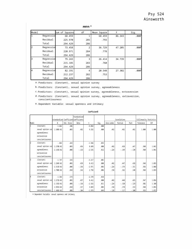
ChartsScatterplot

Dependent Variable: sexual openness and intimacy

Regression Standardized Predicted Value

3210-1-2-3

Reg

ress

ion

Stan

dard

ized

Res

idua

l

4

3

2

1

0

-1

-2

-3

yes the output is the same as the ARC output.b. Compare the output to the output from ARC. Expect there to be a little

difference because they use different estimation methods, but are the two outputs similar?

4. Do a user defined sequential analysis using the block function, predicting soitot by a, e and sos. The order should be a, e and sos, include r-square change and interpret results.


This chart is a little different than the ARC charts because it is looking at the actual predicted y value versus the error (or residual). So instead of looking at every predictor for homoskedasticity it is looking for it on the combined predictors. Again it looks like a little heteroskastic because at low values on the predicted score the errors are mostly positive.


When you ask to save mahalanobis distance it gives you this table which tests a bunch of stuff. Importantly look at the mahal. Distance and see if the maximum exceeds critical chi-square value (in this case with three predictors the crit. value is 16.266) if the maximum doesn’t exceed the crit. value than you have no multivariate outliers. In this case the Max Mahal. Distance is 14.835 so no multivariate outliers. The other entries are other methods to test if values have an undure impact on the equation and are therefore multivariate outliers.

Psy 524Ainsworth

Variables Entered/Removed b

agreeableness a . Enter

egotism a . Enter


a . Enter

Model1

2

3




Model Summary

.050a 14.992 1 285 .000

.000b .000 1 284 .993

.200c 75.467 1 283 .000

Model1

2

3

R Square Change F Change df1 df2 Sig. F Change

Change Statistics

Predictors: (Constant), agreeablenessa.

Predictors: (Constant), agreeableness, egotismb.

Predictors: (Constant), agreeableness, egotism, sexual opinion surveyc.

Coefficients a

1.494 .394 3.790 .000

-3.603E-02 .009 -.224 -3.872 .000

1.488 .702 2.120 .035

-3.605E-02 .010 -.224 -3.782 .000

3.669E-05 .004 .001 .009 .993

-.647 .672 -.964 .336

-2.064E-02 .009 -.128 -2.381 .018

-1.553E-03 .004 -.023 -.428 .669

2.376E-02 .003 .457 8.687 .000

(Constant)

agreeableness

egotism


(Constant)

agreeableness

egotism


(Constant)

agreeableness

egotism


Model1

2

3

B Std. Error


Beta


t Sig.


Excluded Variables c

.001a .009 .993 .001 .957

.456a 8.689 .000 .458 .960

.457b 8.687 .000 .459 .958

egotism


egotism


Model1

2

Beta In t Sig. Partial Correlation Tolerance

CollinearityStatistics

Predictors in the Model: (Constant), agreeablenessa.

Predictors in the Model: (Constant), agreeableness, egotismb.

Dependent Variable: sexual openness and intimacyc.


Tells you which variables were excluded at each step and whether they would have been significant had they been included. Repeats the sentiment earlier, e bad/sos good.


The coefficients and tests for them at each stage. Lets you see how the coefficients change as predictors are added in.


This is the important part. This tells you that the R-square for the first model (a alone) accounts for 5% of soitot and that is significantly different that zero. Tells you that the second model does not improve on the first (adding e does not help a alone) since the R-Squared change for the second model is zero and the sig. is no below .05. The third model is an improvement over the second (sos does improve the prediction by a and e) since the sig. F Change is below .05. Note: the second model is really the same as the first since e added nothing to the prediction of y.


Reminder of what you did. Three step sequential analysis.

Psy 524Ainsworth

5. Do a forward statistical regression and include a, e and sos (include r-squared change) predicting soitot. Interpret results and compare them to the previous result (#4).

RegressionVariables Entered/Removed a


.

Forward(Criterion:Probability-of-F-to-enter <=.050)

agreeableness .


extraversion .


Model1

2

3



Model Summary

.482a .233 .230 .89044 .233 86.343 1 285 .000

.499b .249 .244 .88208 .017 6.425 1 284 .012

.519c .269 .261 .87199 .020 7.609 1 283 .006

Model1

2

3


Change Statistics

Predictors: (Constant), sexual opinion surveya.

Predictors: (Constant), sexual opinion survey, agreeablenessb.

Predictors: (Constant), sexual opinion survey, agreeableness, extraversionc.

ANOVA d

68.459 1 68.459 86.343 .000a

225.970 285 .793

294.429 286

73.458 2 36.729 47.205 .000b

220.971 284 .778

294.429 286

79.243 3 26.414 34.739 .000c

215.185 283 .760

294.429 286

Regression

Residual

Total

Regression

Residual

Total

Regression

Residual

Total

Model1

2

3





Dependent Variable: sexual openness and intimacyd.


The ANOVA summary table for each step, interpreted the same as previous, just in the order determined by the forward sequential entry criterion.


This again tells you the R-squared value for each step (e.g. the percent of variance explained in y by the variables entered at that step. You should interpret R-squared change as the additional prediction added to the previous model. R-square change and R-square are only the same for the first model. Significant R-Square change means that the additional predictors in steps 2 and 3 added to the previous model. When writing this up you would say that SOS accounts for 23% of soitot, agreeableness adds 2% to prediction above sos and extraversion adds another 2% to the prediction above sos and agreeableness


This tells you what type of analysis you performed and the entry criteria (F-to-Enter <= .05). The entry value is the default in SPSS and can be changed in the options command. This also tells you the order of importance of the variables: The sexual opinion survey (sos) enters first so it had the lowest F probability in the first round Agreeableness (a) had the lowest probability in the second round (once sos was already in the equation) And extraversion (e) was significant once sos and a were in the model, or else it wouldn’t have entered.

Psy 524Ainsworth

Coefficients a

-1.862 .206 -9.058 .000

2.508E-02 .003 .482 9.292 .000

-.863 .443 -1.946 .053

2.370E-02 .003 .456 8.689 .000

-2.143E-02 .008 -.133 -2.535 .012

-1.747 .543 -3.217 .001

2.284E-02 .003 .439 8.413 .000

-2.515E-02 .008 -.156 -2.971 .003

2.708E-02 .010 .142 2.758 .006

(Constant)


agreeableness

extraversion

(Constant)


agreeableness

extraversion

(Constant)


agreeableness

extraversion

Model1

2

3

B Std. Error


Beta


t Sig.


Excluded Variables c

-.133a -2.535 .012 -.149 .960

.118a 2.284 .023 .134 .993

.142b 2.758 .006 .162 .968

agreeableness

extraversion

agreeableness

extraversion

Model1

2

Beta In t Sig. Partial Correlation Tolerance

CollinearityStatistics

Predictors in the Model: (Constant), sexual opinion surveya.

Predictors in the Model: (Constant), sexual opinion survey, agreeablenessb.

Dependent Variable: sexual openness and intimacyc.

6. Do a stepwise regression including sos, ego, n, e, o, a and c predicting soitot. Include estimates, model fit, r squared change, descriptives, part and partial correlations, collinearity diagnostics, a plot of zpred (x) and zresid (y), and save mahalanobis distances. Interpret and annotate the output.

RegressionDescriptive Statistics

-.0155 1.01463 287

73.6237 19.51110 287

163.1864 14.75218 287

36.948 7.1976 287

40.728 5.3385 287

40.456 5.8355 287

41.878 6.2948 287

41.983 7.0728 287



egotism

neroticism

extraversion

openness

agreeableness

conscientiousness

Mean Std. Deviation N


Descriptives – not too much to interpret


Excluded variables and whether they would have also been significant if they were entered in the step. Shows the relative ordering of the excluded variables and you can see why a entered before e, etc.


Coefficient table – shows how the model changes as predictors are added. You should interpret the values of the Bs and track the size of the variables throughout the steps (e.g. sos gets smaller so there is relationship between it and the other variables being accounted for in the second and third steps.

Psy 524Ainsworth

Correlations

1.000 .482 -.046 -.123 .158 .089 -.224 -.128

.482 1.000 .007 -.098 .084 .191 -.199 -.048

-.046 .007 1.000 .013 .010 .390 .208 .087

-.123 -.098 .013 1.000 -.238 .017 -.038 -.262

.158 .084 .010 -.238 1.000 .033 .139 .168

.089 .191 .390 .017 .033 1.000 .055 -.019

-.224 -.199 .208 -.038 .139 .055 1.000 .217

-.128 -.048 .087 -.262 .168 -.019 .217 1.000

. .000 .218 .019 .004 .067 .000 .015

.000 . .453 .049 .077 .001 .000 .210

.218 .453 . .415 .431 .000 .000 .071

.019 .049 .415 . .000 .388 .258 .000

.004 .077 .431 .000 . .290 .009 .002

.067 .001 .000 .388 .290 . .177 .372

.000 .000 .000 .258 .009 .177 . .000

.015 .210 .071 .000 .002 .372 .000 .

287 287 287 287 287 287 287 287

287 287 287 287 287 287 287 287

287 287 287 287 287 287 287 287

287 287 287 287 287 287 287 287

287 287 287 287 287 287 287 287

287 287 287 287 287 287 287 287

287 287 287 287 287 287 287 287

287 287 287 287 287 287 287 287



egotism

neroticism

extraversion

openness

agreeableness

conscientiousness



egotism

neroticism

extraversion

openness

agreeableness

conscientiousness



egotism

neroticism

extraversion

openness

agreeableness

conscientiousness

Pearson Correlation

Sig. (1-tailed)

N

sexual opennessand intimacy

sexual opinionsurvey egotism neroticism extraversion openness agreeableness conscientiousness


Correlations between all of the variables with significance values. Not too much to interpret but a good place to start looking for multicollinearity/singularity and none of them seem to be even near violation.

Psy 524Ainsworth

Variables Entered/Removed a


.

Stepwise(Criteria:Probability-of-F-to-enter <=.050,Probability-of-F-to-remove>= .100).

agreeableness .


extraversion .


conscientiousness .


Model1

2

3

4



Model Summary e

.482a .233 .230 .89044 .233 86.343 1 285 .000

.499b .249 .244 .88208 .017 6.425 1 284 .012

.519c .269 .261 .87199 .020 7.609 1 283 .006

.528d .279 .269 .86753 .010 3.917 1 282 .049

Model1

2

3

4


Change Statistics




Predictors: (Constant), sexual opinion survey, agreeableness, extraversion, conscientiousnessd.

Dependent Variable: sexual openness and intimacye.


At each step the R-square change shows that each new variables adds significantly to the prediction. Just barely for conscientiousness (c) (the last step).


Tells you the order in which variables enter and are removed. None of the variables leave once entered which means that at no point does an entered variable’s F probability drop below .10. It also tells you that out of all of the variables you included only these for significantly predict soitot. The relative order of importance is sos, a, e and c.

Psy 524Ainsworth

ANOVA e

68.459 1 68.459 86.343 .000a

225.970 285 .793

294.429 286

73.458 2 36.729 47.205 .000b

220.971 284 .778

294.429 286

79.243 3 26.414 34.739 .000c

215.185 283 .760

294.429 286

82.191 4 20.548 27.302 .000d

212.237 282 .753

294.429 286

Regression

Residual

Total

Regression

Residual

Total

Regression

Residual

Total

Regression

Residual

Total

Model1

2

3

4





Predictors: (Constant), sexual opinion survey, agreeableness, extraversion,conscientiousness

d.


Coefficients a

-1.862 .206 -9.058 .000

2.508E-02 .003 .482 9.292 .000 .482 .482 .482 1.000 1.000

-.863 .443 -1.946 .053

2.370E-02 .003 .456 8.689 .000 .482 .458 .447 .960 1.041

-2.143E-02 .008 -.133 -2.535 .012 -.224 -.149 -.130 .960 1.041

-1.747 .543 -3.217 .001

2.284E-02 .003 .439 8.413 .000 .482 .447 .428 .948 1.055

-2.515E-02 .008 -.156 -2.971 .003 -.224 -.174 -.151 .936 1.068

2.708E-02 .010 .142 2.758 .006 .158 .162 .140 .968 1.033

-1.364 .574 -2.378 .018

2.272E-02 .003 .437 8.412 .000 .482 .448 .425 .947 1.056

-2.192E-02 .009 -.136 -2.555 .011 -.224 -.150 -.129 .902 1.108

2.991E-02 .010 .157 3.029 .003 .158 .178 .153 .948 1.055

-1.486E-02 .008 -.104 -1.979 .049 -.128 -.117 -.100 .933 1.072

(Constant)


agreeableness

extraversion

conscientiousness

(Constant)


agreeableness

extraversion

conscientiousness

(Constant)


agreeableness

extraversion

conscientiousness

(Constant)


agreeableness

extraversion

conscientiousness

Model1

2

3

4

B Std. Error


Beta


t Sig. Zero-order Partial Part

Correlations

Tolerance VIF




Also interpreted the same. Values change when new variables enter showing relationships between the predictors. If you look closely you can see some interesting things happening. When extraversion enters agreeableness actually gets more negative (maybe suppression, I don’t know)


Anova table is interpreted the same way

Psy 524Ainsworth

Excluded Variables e

-.049a -.952 .342 -.056 1.000 1.000 1.000

-.076a -1.462 .145 -.086 .990 1.010 .990

.118a 2.284 .023 .134 .993 1.007 .993

-.003a -.063 .950 -.004 .964 1.038 .964

-.133a -2.535 .012 -.149 .960 1.041 .960

-.105a -2.027 .044 -.119 .998 1.002 .998

-.023b -.428 .669 -.025 .954 1.048 .917

-.084b -1.631 .104 -.096 .987 1.013 .949

.142b 2.758 .006 .162 .968 1.033 .936

.010b .182 .856 .011 .955 1.047 .920

-.081b -1.536 .126 -.091 .953 1.050 .917

-.019c -.364 .716 -.022 .954 1.049 .893

-.055c -1.051 .294 -.062 .937 1.067 .919

.009c .179 .858 .011 .955 1.047 .908

-.104c -1.979 .049 -.117 .933 1.072 .902

-.014d -.271 .787 -.016 .951 1.051 .865

-.085d -1.578 .116 -.094 .884 1.132 .880

.006d .116 .908 .007 .954 1.049 .893

egotism

neroticism

extraversion

openness

agreeableness

conscientiousness

egotism

neroticism

extraversion

openness

agreeableness

conscientiousness

egotism

neroticism

extraversion

openness

agreeableness

conscientiousness

egotism

neroticism

extraversion

openness

agreeableness

conscientiousness

Model1

2

3

4

Beta In t Sig. Partial Correlation Tolerance VIFMinimumTolerance


Predictors in the Model: (Constant), sexual opinion surveya.

Predictors in the Model: (Constant), sexual opinion survey, agreeablenessb.

Predictors in the Model: (Constant), sexual opinion survey, agreeableness, extraversionc.

Predictors in the Model: (Constant), sexual opinion survey, agreeableness, extraversion, conscientiousnessd.



Interpreted the same. Relative importance of excluded variables at each step. Tolerance values are all really large indicating no multicollinearity.

Psy 524Ainsworth

Collinearity Diagnostics a

1.967 1.000 .02 .02

3.326E-02 7.690 .98 .98

2.936 1.000 .00 .01 .00

5.527E-02 7.289 .01 .72 .12

8.524E-03 18.559 .99 .27 .88

3.920 1.000 .00 .00 .00 .00

5.779E-02 8.236 .00 .77 .08 .01

1.540E-02 15.956 .00 .11 .57 .57

6.459E-03 24.637 .99 .12 .35 .41

4.896 1.000 .00 .00 .00 .00 .00

6.220E-02 8.873 .00 .76 .04 .00 .03

2.011E-02 15.605 .01 .00 .22 .05 .88

1.534E-02 17.866 .00 .11 .47 .62 .01

6.156E-03 28.203 .99 .13 .26 .33 .07

Dimension1

2

3

4

5

1

2

3

4

5

1

2

3

4

5

1

2

3

4

5

Model1

2

3

4

Eigenvalue Condition Index (Constant)sexual opinion

survey agreeableness extraversion conscientiousness

Variance Proportions


Casewise Diagnostics a

3.839 3.69

3.362 2.23

Case Number127

199

Std. Residualsexual openness

and intimacy


Residuals Statistics a

-1.6846 1.4339 -.0155 .53608 287

-3.114 2.704 .000 1.000 287

.05827 .20872 .11020 .03115 287

-1.7043 1.3557 -.0154 .53741 287

-1.9009 3.3307 .0000 .86145 287

-2.191 3.839 .000 .993 287

-2.212 3.857 .000 1.001 287

-1.9373 3.3617 .0000 .87624 287

-2.228 3.956 .002 1.007 287

.294 15.558 3.986 2.905 287

.000 .054 .003 .007 287

.001 .054 .014 .010 287

Predicted Value

Std. Predicted Value

Standard Error ofPredicted Value

Adjusted Predicted Value

Residual

Std. Residual

Stud. Residual

Deleted Residual

Stud. Deleted Residual

Mahal. Distance

Cook's Distance

Centered Leverage Value

Minimum Maximum Mean Std. Deviation N



Same as earlier. Now the critical value is 18.467 because it calculates the mahal. Distance for only those variables that enter (there are 4 of them). So there are no multivariate outliers (the max is 15.558)


Not important


No condition index is above 30 so there is no problem with multicollinearity.

Psy 524Ainsworth

ChartsScatterplot

Dependent Variable: sexual openness and intimacy

Regression Standardized Predicted Value

3210-1-2-3-4

Reg

ress

ion

Stan

dard

ized

Res

idua

l

4

3

2

1

0

-1

-2

-3

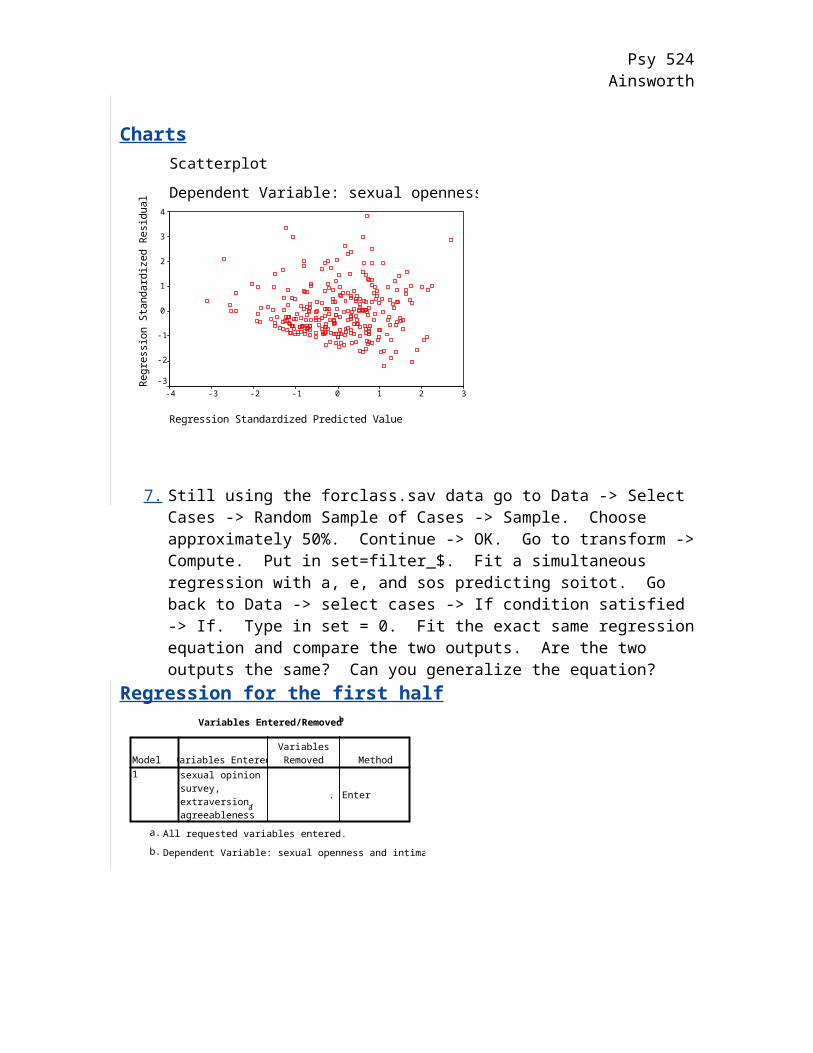
7. Still using the forclass.sav data go to Data -> Select Cases -> Random Sample of Cases -> Sample. Choose approximately 50%. Continue -> OK. Go to transform -> Compute. Put in set=filter_$. Fit a simultaneous regression with a, e, and sos predicting soitot. Go back to Data -> select cases -> If condition satisfied -> If. Type in set = 0. Fit the exact same regression equation and compare the two outputs. Are the two outputs the same? Can you generalize the equation?

Regression for the first halfVariables Entered/Removed b


a. Enter

Model1




Model Summary

.545a .297 .282 .92738Model1

R R Square Adjusted R SquareStd. Error ofthe Estimate

Predictors: (Constant), sexual opinion survey, extraversion,agreeableness

a.


Still showing heteroskedasticity even with more predictors.

Psy 524Ainsworth

ANOVA b

52.969 3 17.656 20.530 .000a

125.564 146 .860

178.533 149

Regression

Residual

Total

Model1




Coefficients a

-2.286 .804 -2.843 .005

-2.588E-02 .012 -.155 -2.117 .036

3.774E-02 .015 .180 2.547 .012

2.496E-02 .004 .439 6.008 .000

(Constant)

agreeableness

extraversion


Model1

B Std. Error


Beta


t Sig.


Regression for second halfVariables Entered/Removed b


a. Enter

Model1




Model Summary

.489a .239 .221 .81266Model1


Predictors: (Constant), sexual opinion survey, extraversion,agreeableness

a.

ANOVA b

27.531 3 9.177 13.896 .000a

87.835 133 .660

115.367 136

Regression

Residual

Total

Model1




Psy 524Ainsworth

Coefficients a

-1.267 .734 -1.725 .087

-2.217E-02 .012 -.144 -1.866 .064

1.604E-02 .013 .095 1.239 .218

2.045E-02 .004 .441 5.772 .000

(Constant)

agreeableness

extraversion


Model1

B Std. Error


Beta


t Sig.


When I did it I got slightly different R-squared values which says the equation may not generalize and the regression coefficients are different for the two models which also says it may not generalize.

8. Centering and Interactions. Open social2.sav in SPSS.a. Recode gender so that males = 0 and females = 1. b. Center both ciccomp and oocomp separately (ciccent and oocent)c. Predict oocent with gender and ciccent and interpret results (don’t forget

to interpret the intercept since it is meaningful).Variables Entered/Removed b

GENDER,CICCENT

a . Enter

Model1



Dependent Variable: OOCENTb.

Model Summary

.443a .197 .190 4.18239Model1


Predictors: (Constant), GENDER, CICCENTa.

ANOVA b

1079.195 2 539.597 30.847 .000a

4408.092 252 17.492

5487.286 254

Regression

Residual

Total

Model1


Predictors: (Constant), GENDER, CICCENTa.



Significant prediction


Ciccent and gender account for 20% of the variance in oocent


Tells you the method is enter and labels the predictors


Use compute function and subtract each variables mean from itself

Psy 524Ainsworth

Coefficients a

-.582 .350 -1.664 .097

.203 .028 .406 7.169 .000

1.459 .529 .156 2.760 .006

(Constant)

CICCENT

GENDER

Model1

B Std. Error


Beta


t Sig.

Dependent Variable: OOCENTa.

d. Cross multiply gender (0 and 1) and ciccent to make a new variable gen_cic.

e. Predict oocent by gender (0 and 1), ciccent and gen_cic. Interpret the results.

RegressionVariables Entered/Removed b

GEN_CIC,GENDER,CICCENT

a. Enter

Model1




Model Summary

.444a .197 .187 4.19049Model1


Predictors: (Constant), GEN_CIC, GENDER, CICCENTa.

ANOVA b

1079.676 3 359.892 20.495 .000a

4407.611 251 17.560

5487.286 254

Regression

Residual

Total

Model1


Predictors: (Constant), GEN_CIC, GENDER, CICCENTa.


Coefficients a

-.581 .351 -1.657 .099

1.463 .530 .156 2.759 .006

.207 .037 .413 5.573 .000

-9.538E-03 .058 -.012 -.165 .869

(Constant)

GENDER

CICCENT

GEN_CIC

Model1

B Std. Error


Beta


t Sig.

Dependent Variable: OOCENTa.


The main point is here, there is no significant interaction between gender and ciccent. Which mean the relationship between ciccent and oocent is the same for men and women


Both are significant predictors of oocent. The constant here is the value of y for men who are at the mean on ciccent. Men at the mean on ciccent are below the mean on the outcome variable. The B for ciccent is interpreted in the usual way The B for gender states that the mean difference between men and women on oocent. As gender moves from 0 to 1 you add 1.459, etc.

Psy 524Ainsworth

9. Mediation using regression. Open social2.sav in SPSS and perform a mediational analysis using oocomp as the predictor, ciccomp as the mediator and qdicomp as the outcome. Interpret the results. Refer to the four steps from the powerpoint slides.


OOCOMP a . EnterModel1



Dependent Variable: QDICOMPb.

Model Summary

.315a .099 .096 3.48964Model1


Predictors: (Constant), OOCOMPa.

ANOVA b

342.701 1 342.701 28.142 .000a

3117.464 256 12.178

3460.164 257

Regression

Residual

Total

Model1




Coefficients a

16.768 1.030 16.277 .000

.242 .046 .315 5.305 .000

(Constant)

OOCOMP

Model1

B Std. Error


Beta


t Sig.

Dependent Variable: QDICOMPa.


OOCOMP a . EnterModel1



Dependent Variable: CICCOMPb.


The regression coefficient is significant


Step 1: Oocomp sig. predicts qdicomp


About 10% of the variance in qdicomp explained by oocomp

Psy 524Ainsworth

Model Summary

.444a .198 .194 8.49284Model1



ANOVA b

4545.723 1 4545.723 63.023 .000a

18464.859 256 72.128

23010.582 257

Regression

Residual

Total

Model1



Dependent Variable: CICCOMPb.

Coefficients a

48.257 2.507 19.249 .000

.883 .111 .444 7.939 .000

(Constant)

OOCOMP

Model1

B Std. Error


Beta


t Sig.

Dependent Variable: CICCOMPa.


CICCOMP,OOCOMP

a . Enter

Model1




Model Summary

.535a .286 .281 3.11191Model1


Predictors: (Constant), CICCOMP, OOCOMPa.

ANOVA b

990.756 2 495.378 51.155 .000a

2469.408 255 9.684

3460.164 257

Regression

Residual

Total

Model1


Predictors: (Constant), CICCOMP, OOCOMPa.



Both ciccomp and oocomp account for 54% of the variance in qdicomp


Significant B


Step 2: Ciccomp sig. predicts oocomp


About 44% of the variance in oocomp is accounted for by ciccomp

Psy 524Ainsworth

Coefficients a

7.727 1.437 5.377 .000

7.699E-02 .045 .100 1.693 .092

.187 .023 .483 8.180 .000

(Constant)

OOCOMP

CICCOMP

Model1

B Std. Error


Beta


t Sig.

Dependent Variable: QDICOMPa.

10. In the social2 data set the variables are:1 ciccomp classroom interracial climate2 qdicomp discrimination index3 srchcomp ethnic identity search4 eicomp ethinic identity strength5 subcomp subgroup identity6 oocomp outgroup orientation7 supcomp superordinate identity

a. Think of a possible hypothesis for how these variables might predict one another (e.g. pick a DV and a few IVs and make up a reason why they might be related) in a use defined sequential regression analysis.

b. Perform all appropriate tests on the variables (assumptions, transformations when needed,etc).

c. Perform the sequential analysis using SPSS. Interpret the resultsd. On a separate sheet of paper write the hypothesis in a couple of sentences max

and then write an APA style results section summarizing your results (refer to the end of chapter 5 for a couple of samples). Make sure to write the results so that anyone reading it can understand it (make it as clear as possible and in very simple language, explaining all technical terms).

This answer is different for everyone so there is no real way to answer it here.


Step 3: this shows that there is full mediation because when oocomp and ciccomp are in together oocomp no longer predicts qdicomp significantly.

lab #3 - california state university, northridgeata20315/psy524/docs/psy524 lab 3 (answers... ·...

Documents