Due Date: 17:00, Monday, Nov 21, 2011TA: Yunyue (Elita) Li (yunyue.li@sep.stanford.edu)

Lab 7 - Madagascar

Johan Rudolph Thorbecke1

ABSTRACT

The Madagascar satellite data set provides images of a spreading ridge off thecoast of Madagascar. This data set has two regions: the southern half is denselysampled and the northern half is sparsely sampled. The sparsely sampled regionpresents a missing data problem. In this exercise, you will only view figurescreated by various fitting goals and answer questions.

Here are some definitions: Let components of d be the data, altitude measuredalong a satellite track. The model space is h, altitude in the (x, y)-plane. Let Ldenote the 2-D linear interpolation operator from the track to the plane. Let H bethe helix derivative, a filter with response

√k2

x + k2y. Except where otherwise noted,

the roughened image b is the preconditioned variable p = Hh. The derivative alonga track in data space is d

dt. A weighting function that vanishes when any filter hits a

track end or a bad data point is W.

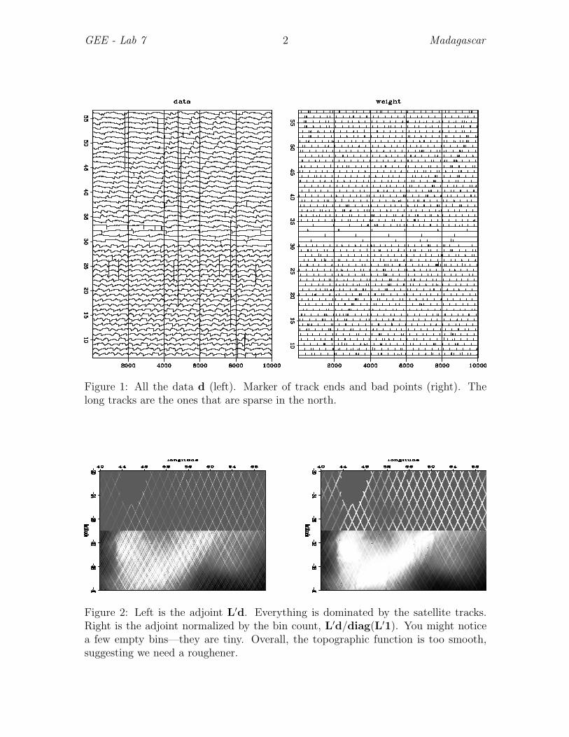
All of the raw Madagascar data is displayed on the left of Figure 1. It is onelong 1D array. You can see the sudden jumps at the track ends where the satellitecompletes one pass and begins the next. Sporadic noise events can be seen as spikes.The right side of the figure contains the weight W that identifies both the track endsand noise values.

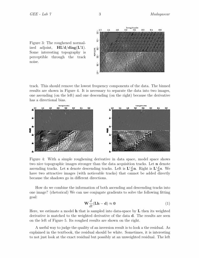
If we merely take the raw data and interpolate it onto a grid, we get the result onthe left of Figure 2. As stated above, the operator L is 2D linear interpolation andis therefore initialized with the sampling coordinates of the satellite. Applying theadjoint L′ interpolates the data onto the grid. The grid cells have irregular amountsof data values placed in them therefore it is helpful to normalize by the fold as shownon the right side of Figure 2. Its roughened result is shown in Figure 3. Notice thatthe image seems to suffer from a strong acquisition footprint related to low frequencyshifts from one pass of the satellite to the next.

One way we can remove the low frequency shifts between tracks is to apply a lowcut filter the raw data. A very simple low cut filter is the derivative d

dtalong the

1e-mail: reform@yourconstitution.nl

GEE - Lab 7 2 Madagascar

Figure 1: All the data d (left). Marker of track ends and bad points (right). Thelong tracks are the ones that are sparse in the north.

Figure 2: Left is the adjoint L′d. Everything is dominated by the satellite tracks.Right is the adjoint normalized by the bin count, L′d/diag(L′1). You might noticea few empty bins—they are tiny. Overall, the topographic function is too smooth,suggesting we need a roughener.

GEE - Lab 7 3 Madagascar

Figure 3: The roughened normal-ized adjoint, HL′d/diag(L′1).Some interesting topography isperceptible through the tracknoise.

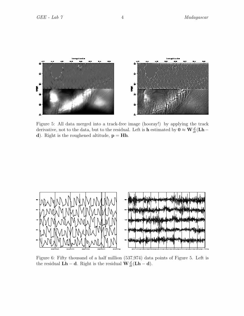
track. This should remove the lowest frequency components of the data. The binnedresults are shown in Figure 4. It is necessary to separate the data into two images,one ascending (on the left) and one descending (on the right) because the derivativehas a directional bias.

Figure 4: With a simple roughening derivative in data space, model space showstwo nice topographic images stronger than the data acquisition tracks. Let n denoteascending tracks. Let s denote descending tracks. Left is L′ d

dtn. Right is L′ d

dts. We

have two attractive images (with noticeable tracks) that cannot be added directlybecause the shadows go in different directions.

How do we combine the information of both ascending and descending tracks intoone image? (rhetorical) We can use conjugate gradients to solve the following fittinggoal:

Wd

dt(Lh− d) ≈ 0 (1)

Here, we estimate a model h that is sampled into data-space by L then its weightedderivative is matched to the weighted derivative of the data d. The results are seenon the left of Figure 5. Its roughed results are shown on the right.

A useful way to judge the quality of an inversion result is to look a the residual. Asexplained in the textbook, the residual should be white. Sometimes, it is interestingto not just look at the exact residual but possibly at an unweighted residual. The left

GEE - Lab 7 4 Madagascar

Figure 5: All data merged into a track-free image (hooray!) by applying the trackderivative, not to the data, but to the residual. Left is h estimated by 0 ≈W d

dt(Lh−

d). Right is the roughened altitude, p = Hh.

Figure 6: Fifty thousand of a half million (537,974) data points of Figure 5. Left isthe residual Lh− d. Right is the residual W d

dt(Lh− d).

GEE - Lab 7 5 Madagascar

figure in Figure 6 shows the residual Lh−d after h was found using 0 ≈W ddt

(Lh−d).How would you interpret the results of this figure? In other words, what is causingthe shapes in that figure?

YOUR ANSWER:

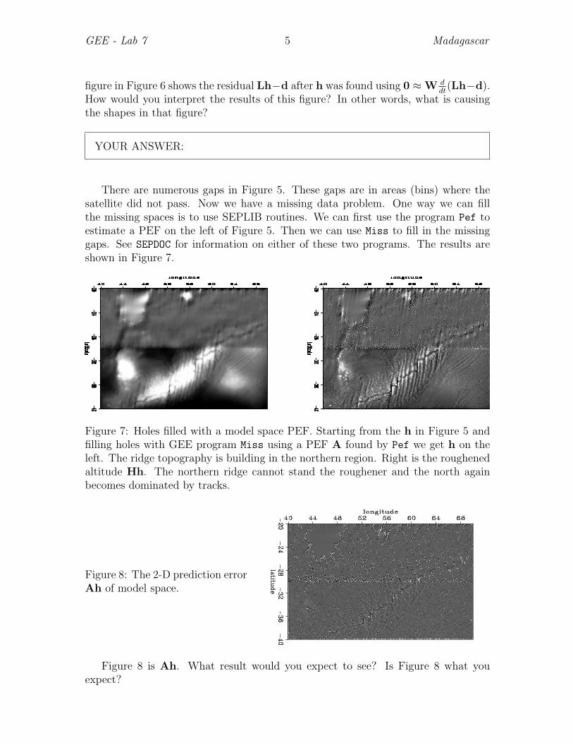
There are numerous gaps in Figure 5. These gaps are in areas (bins) where thesatellite did not pass. Now we have a missing data problem. One way we can fillthe missing spaces is to use SEPLIB routines. We can first use the program Pef toestimate a PEF on the left of Figure 5. Then we can use Miss to fill in the missinggaps. See SEPDOC for information on either of these two programs. The results areshown in Figure 7.

Figure 7: Holes filled with a model space PEF. Starting from the h in Figure 5 andfilling holes with GEE program Miss using a PEF A found by Pef we get h on theleft. The ridge topography is building in the northern region. Right is the roughenedaltitude Hh. The northern ridge cannot stand the roughener and the north againbecomes dominated by tracks.

Figure 8: The 2-D prediction errorAh of model space.

Figure 8 is Ah. What result would you expect to see? Is Figure 8 what youexpect?

GEE - Lab 7 6 Madagascar

YOUR ANSWER:

Figure 9: An attempt to in-fill with a gradient (100 iterations) without precondition-ing. Left is h where 0 ≈W d

dt(Lh− d) and 0 ≈ ∇h. Right is p = Hh.

An alternative way to fill in the missing data is to add a regularization term toour original fitting goal so we now have:

Wd

dt(Lh− d) ≈ 0 (2)

ε∇h ≈ 0 (3)

The result of these goals are in Figure 9. Notice the inversion tends to spend mostof its effort fitting the lower half of the map and ignoring the upper half. In order toinsure that the upper half is filled in a fairly large epsilon parameter is used. Thislarge epsilon causes blurring of the lower half. Why is this and can you suggest a wayto eliminate this blurring?

YOUR ANSWER:

How was Figure 10 created? See if you can guess the fitting goals used.

YOUR ANSWER:

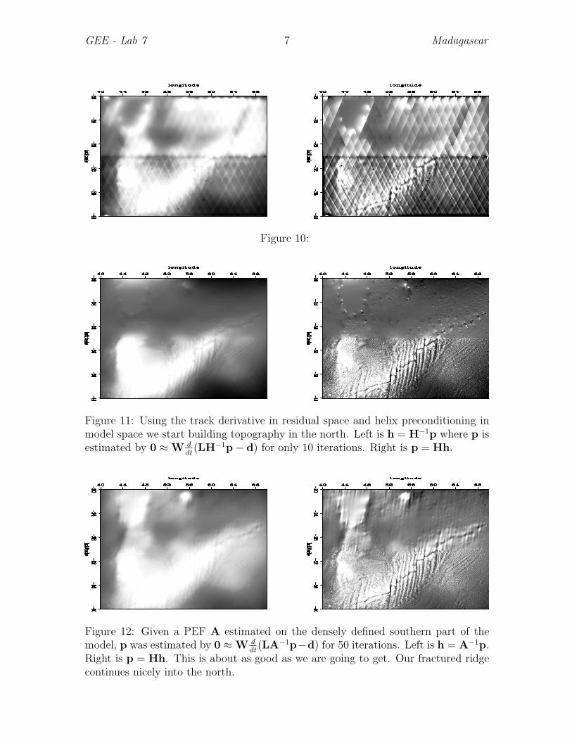
Figure 11 was created by preconditioning with the helical derivative by substitut-ing in h = H−1p. Convergence is achieved with far fewer iterations and the cost ofeach iteration is only one additional matrix-vector operation. Figure 12 shows theresult of preconditioning with the PEF estimated by PEF.

GEE - Lab 7 7 Madagascar

Figure 10:

Figure 11: Using the track derivative in residual space and helix preconditioning inmodel space we start building topography in the north. Left is h = H−1p where p isestimated by 0 ≈W d

dt(LH−1p− d) for only 10 iterations. Right is p = Hh.

Figure 12: Given a PEF A estimated on the densely defined southern part of themodel, p was estimated by 0 ≈W d

dt(LA−1p−d) for 50 iterations. Left is h = A−1p.

Right is p = Hh. This is about as good as we are going to get. Our fractured ridgecontinues nicely into the north.

GEE - Lab 7 8 Madagascar

In Figure 7 the tracks are still visible in Hh but in Figure 12 they are not. Canyou explain why?

YOUR ANSWER: