W TWUHF IV NT NLWUNAB#LTISM LAB F/6 6116MAGNETIC FIELDS OF THE CEREBRAL CORTEX. WIJUN 80 -S J WILLIAMSON. L KAUFMAN N0001,-76-C-0568

dMCLASSIFIED 6 ML

inn/I/Ill/nn

IT.

B I 11111Ll 2 18111i.5

14 11111."~40 _11112.

MICROCOPY RESOLUTION TEST CHART

ECUfITY CLASSIFICATION OF T P

REPORT DOU A 10 B ORE COMPLETING FORM2. GOVT ACCESSION NO LR!MIPIENT S CATALOG NUMBER

4. TITLE (id Subtiiie) S. TYPE OF REPORT A PERIOD COVERED

Magnetic Fields of the Cerebral Cor Publication6. PERFORMING ORG. REPORT NUMBER

SAUTNX . ..... 6. CONTRACT OR GRANT NUM@ER(e)oc) '. / / Samuel Ji illiamson ai6 Lloyd/(aufmj 0- -568. . . . . . . . . . OI" i4-7 6-C

S. PERFORMING ORGANIZATION NAME AND ADDRESS 10. PROGRAM ELEMENT. PROJECT, TASKAREA A WORK UNIT NUMBERS( Dp artments of Physics and Psychology

vWw York University, Washington Square NR 201-209New York, NY 10003

II. CONTROLLING OFFICE NAME AND ADDRESS t2- -REPORT DATE

Office of Naval Research (Code 441)/. 15 Jung 1086Department of the Navy - U.

1-. Arlington. VA 22217 5014. MONITORING AGENCY NAME SiifflI from Controling Office) IS. SECURITY CLASS. (of Ufsi report)

unclassified7 a. GECL ASSI FICATION/ OWNGRADING

SCHEDULE

IS. OISTRIBUTION STATEMENT (of tis. Repo,)

Distribution unlimited D T ICDISTn'UTAON STATEMENT A ELECTE

A :- , uz :.L'iZ: Ieleae; JUL 8 19801 .rn Unlimited

17. DISTRIBUTION STATEMENT (of the absrait entered In Btock 20, it dlff ent tram Report) 111W

A

IS. SUPPLEMENTARY NOTES

To appear in: Biomagnetism, S.N. Ern6, H.D. Hahlbohm, and H.Labbig, Eds.(Walter de Gruyter, Berlin), to be published.

II. KEY WORDS (Continue on reverse side It n*ceemp and idntlfy by block numbet)

biomagnetism vision0 neuromagnetism hearing

evoked potentials touch. evoked magnetic fields cortical sources

20. AmIsT T (Continue an revee old I necesary anfd dentify by beek ambr)

LA- The observed patterns over the scalp of magnetic fields evoked byvisual, somatic, and auditory stimuli are analyzed to deduce the position

S and depth of the equivalent current dipole generating source. Expressionsare developed for both sphere and half space models for the head, andgraphs are presented to correct for the use of a pickup coil of finitediameter. For all three responses, the position of the generating souceis deduced to lie in the corresponding primary projection area of the cort.

DD I F 1473 EDITION OF I NOV 60 IS OBSOLETESWl 0102-LF-0146601

SICUI TY CLASSIFICATION OF THIS PARE a

MAGNETIC FIELDS OF THE CEREBRAL CORTEX* * .

Juiti .f i ,i-' io -.--.---

Samuel J. Williamsont and Lloyd Kaufman Ju__

Neuromagnetism Laboratory , -1Departments of Physics and Psychology i CtesNew York University Aval, ndOrNew York, NY, 10003, U.S.A.

kv1 special

Dlist

Introduction

This paper focuses on several aspects of neuromagnetic studies

of human cortical activity that have proven of particular

interest within the last three years. Although we shall refer

to each of the papers published so far in the area of magneticstudies of brain activity, our treatment is not in the nature

of a review. Elsewhere we shall publish a critical review

of all the work in neuromagnetism to date, including cor-

parisons with the more conventional studies of electric poten-

tial variations on the scalp (1). The reader is also referred

to a complete review of the subject of biomagnetism recently

prepared by the present authors which includes a systematic

and detailed presentation of the basic theory, experimental

techniques, and phenomena (2). An earlier review of biomag-

netism has been given by Williamson, Kaufman, and Brenner (3),and a more specialized review of magnetic phenomena of the

central nervous system has been authored by Reite and

Zimmerman (4).

Background

About 110 years ago Paul Broca found a lesion in the frontal

cortex of the right hemisphere of a speechless man's brain.

This discovery launched a long search to define the

80 7 3 066

relationship between various structures of the brain and

specific psychological functions. While the findings

resulting from this search have shown that various portions

of the brain are related to specific mental processes, none

of them have indicated how the brain really works. What is

it that a particular structure actually does? Recognizing

this problem, psychologists turned to indirect methods in

order to discover the answer. For example, the Gestalt

psychologists promulgated the doctrine of psychophysical iso-

morphism which holds that there is a one-to-one relationship

between occurrences in the brain and events in perception.

They believed that it is possible, from knowledge of states

of the brain, to predict what the owner of the brain actually

perceives. Since it was not then possible to determine

states of the brain, the Gestaltists turned the problem

around. Their doctrine enabled them to say that one could

discover the states of the brain by studying the perfectly

correlated states of perceptual experience. Unfortunately,

the program of the Gestalt psychologists foundered on the

fact that there appears to be no unique way to determine

precisely what it is that the brain does from'a study 'of

what it is that the owner of the brain experiences. Ongoing

brain processes are far more complicated than what an obser-

ver is capable of reporting about his experiences.

Even though there is no way to uniquely determine the brain

functions that underly perceptual experience from the study

of that experience alone, there have been a number of fruit-

ful guesses. This is not too surprising since neural events

do underly perceptual phenomena and some of these phenomena,

when properly studied, suggest basic functional mechanisms

whose existence may be verified by physiological means.

There are a number of famous examples in which physiological

mechanisms were predicted by means of psychological methods.

For one, the trichromaticity theory proposed by Maxwell and

Helmholtz to account for the facts of color mixture led to

the prediction of the existence of three types of cones, each

type with its own spectral response properties. The particu-

lar absorption spectra were identified in psychophysical

experiments and were subsequently verified by direct physio-

logical measurements. Alpo, the opponent mechanisms that are

now known to be present in the visual system were first pos-

tulated by Hering to account for certain phenomena in color

vision. The response properties of these mechanisms were

identified in psychophysical experiments before actual neurons

having the same properties were studied by physiological

means. Finally, certain visual phenomena suggested the exis-

tence of an inhibitory process because the sensation gotten

by stimulation of one retinal place is altered when another

retinal place is simultaneously stimulated. This led to the

discovery of lateral inhibition in the eye of an inverte-

brate animal.

The psychophysical methods used to measure the sensitivity

of the visual system to various kinds of stimuli and how

this sensitivity varies with the conditions of the experi-

ment have been very useful in suggesting mechanisms at various

stages in the visual system. These stages involve the

photoreceptors, the peripheral neurons and the afferent path-

ways, and even the brain itself.

Another method often used by psychologists in their investi-

gations of sensory systems is the reaction time method which

was first developed by Helmholtz. The total reaction time

depends upon the time constants of the receptors, the peri-

pheral neural pathways, and the brain, as well as the time for

signals to traverse the efferent neural pathways and cause

muscles to contract. The peripheral and the central compon-

ents involved in the overall reaction time task are notor-

iously variable. Reaction time is influenced by the expec-

tancy of the subject, his state of alertness and, among other

things, the method employed in presenting the stimulus (5).

Despite these difficulties, modern psychologists have been

successful in drawing inferences from the reaction time method

about the organization of sensory systems. These inferences,

as with those made on the basis of measures of sensitivity,

require verification in the physiological domain. There is

a need for converging experiments in which the methods of

psychology and of physiology are both used to evaluate

theories concerning the functions that underly perception.

in the past few decades the physiologists developed an extra-

ordinarily powerful tool for investigating the properties

of the sensory systems of animals. This is the micro-

electrode which is so small that it can sense the activity

of a single neuron when it is placed alongside it. Studies

of cells within the brain of a living animal led to the

astounding discovery that some of them respond to specific

types of visual stimuli. Some cells respond- to lines or

bars of particular orientation, others to moving objects

and still others to corners. We shall not go into the details

of the many discoveries made possible by means of the micro-

electrode. It is sufficient to say that these discoveries

created considerable ferment among perceptionists because

they suggested that many of the cells have the properties

of mechanisms that could underly sensory phenomena. We shall

consider but one example here.

Cells in the retina of the cat, for example, may be sub-

divided into at least two types. one type responds to rela-

tively large stimuli that are presented rapidly to the eye.

These are referred to as Y-cells or, sometimes, as transient

cells. Another type responds to fine ddtails and are most

sensitive to fine patterns when they are moved slowly or

presented steadily. They are the so-called K-cells (sus-

tained cells) and are believed to be involved in pattern

vision. These results in animals are analogous to psycho-physical findings in humans (6). It is clear that some means

is needed for physiological verification of the presence of

sustained and transient channels in the human visual system.

One physiological measure that can be used with humans is

that of detecting potential differences between electrodes

attached to the scalp.

Early in this century physiologically oriented scientists

sought a direct measure of human brain activity in the hope

that it would reveal the locations and mechanisms that

underly mental phenomena. The discovery in the 1920s that

potential differences between electrodes attached to the

scalp fluctuate over time led to the clinically useful

characterization of types of potential changes. This dis-

covery of the electroencephalogram was followed by thefinding that stimulation of the eyes,1 the ears and the skin

can lead to detectable electrical responses of the brain.

In more recent years these evoked potentials in the case of

visual stimuli were found to be differentially affected by

patterns as opposed to mere changes in the level of illumi-

nation of the eye (7). Also, the amplitudes of components

of the evoked potential are differentially affected by the

state of arousal of'the subject. Despite these discoveries,

it is still difficult to identify the sources of many com-ponents of the evoked responses which may well originate in

different parts of the brain. It is clearly necessary to

discover wherther the components of the complex waveform

composing the evoked potential originate in different

structures and to what degree they are independent of each

other.

The evoked potential is a very coarse measure. Distant popu-

lations of cells in the cortex as well as subcortical nuclei

of the brain affect electrodes at the scalp because of currents

that spread throughout the medium of the brain. These so-

called volume currents are so widespread that the signals

of widely separated populations become intermixed and their

individual behavior cannot be separated or resolved. This

limitation is unfortunate, because even though it is possible

to perform many ingenious experiments, the interpretation

of their results in terms of findings with microelectrodesis highly speculative. A given effect might be due to the

average activity of diverse populations of cells with very

different functions. This may be why studies of the evokedvoltages between a pair of electrodes generally have not been

able to localize the position of the source. One exception

is - the signal corresponding to the first activity in the

cortex, several tens of milliseconds following stimulation.

Later we shall cite recent studies using multi-electrode

arrays which appear to offer better resolution of later

activity in the cortex. Nevertheless, the few instances

where it has been possible to establish the location of a

source have revealed virtually nothing about the functional

aspects of cortical activity, viz, how sensory information

is processed. As we shall see, the evoked magnetic response

may help ameliorate this problem.

Our understanding of higher levels of brain processes is

even more primitive. From a clinical standpoint the electro-

encephalogram (EEG) which characterizes onoing electrical

activity has proved valuable in diagnosing certain disorders.

But very little is known about the'sources of these

signals or the role of the underlying neural processes.

It is not even known whether the EEG contains substantive

information related to thought processes or memory. Despite

considerable effort in this kind of study, its contributions

toward revealing functional aspects of the brain are meager.

The earliest measurements of the magnetic fields associated

with brain activity were dedicated to studies of this spon-

taneous activity, as expressed by the magnetoencephalogram

(MEG). This includes work by Cohen (8,9), Reite et al. (10),

and Hughes et al. (11, 12). There are some correlations

between the temporal and spatial characteristics of the MEG

and EEG, especially with regard to the alpha rhythm. But

other features display very weak correlations at best. As

our purpose in this paper is to consider aspects of cortical

activity, we will not discuss these features of the spontan-

eous MEG that, though interesting, are not clearly of cortical

origin. The reader is referred to the original reports and

to three review papers which highlight the similarities and

differences (1,2,4) between MEG and EEG measures of spon-

taneous activity.

Aspects of Instrumentation

As will later become clear there is considerable interest

in mapping the pattern of magnetic field in some detail

near the scalp. To achieve this, either the subject must

move about from one position to another or the magnetic

sensor must be moved. For'neuromagnetic studies, acceptable

field sensitivity at low frequencies can be obtained only

by use of a sensor based on the superconducting quantum

interference device (SQUID). The SQUID and the

superconducting detection coil which directly senses the

field of interest are kept at low temperature by immersion

in a bath of liquid helium contained within a cryogenic

dewar. A contemporary dewar is a rather bulky object because

to conserve liquid helium it is designed to provide good

thermal insulation and,to minimize the frequency of refilling,

it has a modest storage capacity of perhaps 5 liters for

several days supply. Nevertheless there are cases where it

is not feasible to disturb the subject, and the dewar must

be moved. Mapping a field pattern over the scalp becomes

a tedious process unless the dewar's suspension is suffi-

ciently flexible. Using three SQUID systems and an orthogonal

set of magnetometer coils in the tail of the dewar to detect

the three components of the neuromagnetic field would mini-

mize the need to physically reorient the dewar when measuring

the field in various directions. But more complicated coil

geometries, such as the second-order gradiometer which has

proven useful for measurements in an unshielded environment,

have yet to be adapted to multiple axis configurations.

Therefore the dewar must be both displaced and oriented to

affect measurements about the head.

The well known method of mounting the dewar in a two-axis

gimballed support is useful but suffers from an inherent

disadvantage whereby the detection coil in the tail of the

dewar is displaced horizontally when the orientation is

adjusted. A simple design that avoids the worst aspect of

displacement is portrayed in the photograph in Pig. 1.

The details are sketched in Fig. 2. The dewar is held in a

fiberglass cradle which is suspended from an aluminum carriage

free to travel horizontally on two sets of orthogonally

oriented tracks. The tracks are ground stainless steel

rods, and the carriage is supported on them by linear motion

Thompson roller bearings. A horizontal run of %"40 cm. in

each direction is possible; and when the desired position

is reached the carriage is locked with spring-loaded bicycle

brakes (not shown). To minimize any transmission of building

vibrations to the dewar, the suspension supported by the

carriage is fabricated from fiberglass or wood wherever

possible. Vertical movement of the dewar is permitted by a

6 cm diameter cylindrical axle of hardwood that runs between

sets of aluminum rollers having double conical shape. The

axle is supported by four strands of nylon parachute cord,

each rated for 230 kgthat run over a pully to a lead counter-

weight. The axle has the additional advantage of allowing

rotations about the vertical axis for adjusting the dewar's

azimuthal orientation. Friction in the system holds the

vertical and azimuthal positions.

For adjustment of the dewar's declination by as much as 45 0

from the vertical, a system of gears rotates a fiberglass

frame with respect to a horizontal yoke fixed to the vertical

axle. At the same time the dewar is rotated with respect

to the frame in the opposite direction. The frame is

Figure 1. Installation at New York University for measuringevoked magnetic fields of the human brain. The SQUID detec-tion system is mounted within the dewar, suspended over thesubject's head. The detection coil is located within thenarrow tail of the dewar, which in this illustration is posi-tioned to detect the auditory evoked field.

carriage puffy linear

Idwarriae omotion

beari ndr n

to scale.s see

r,, tracks,.]

-- vertical axle

.4 ounterweights isupport

-rome

yoke

sfixed gear

lclimbing gear

\ ,v 'worm

d~d declination oxle /

ewor cradle

--- ewor

Figure 2. A suspension system permitting translation of adewar in any of three orthogonal directions and adjustmentof the dewar's declination and azimuth without horizontaldisplacement of the bottom of the dewar. The drawing is notto scale.

counterweighted to minimize the torque required for driving

the gears. To effect this rotation a crank and shaft rotate

worms which mesh with worm gears on two separate horizontal

shafts. One shaft (the declination axle) near the end of

the frame rotates the dewar. The other near the center of

the frame rotates a pair of climbing gears that mesh with

gears fixed to the ends of the yoke. As they rotate they"climb" up or down the fixed gears and thereby rotate the

frame. If the dewar is mounted in the carriage so that the

distance between the bottom of its tail and the declination

axle matches the distance between that axle and the center

of the fixed gears,--the bottom of the tail remains precisely

under the vertical axle. Thus any adjustments of declination

or azimuth leave the bottom of the tail at the same horizon-

tal position, as desired. One disadvantage of this simple

arrangement is the fact that as the dewar's declination is

adjusted the height of the dewar also changes, thereby

requiring a compensating adjustment of the position of the

vertical axle. In practice this is a small price to pay

for the convenience in maintaining the horizontal position

during angular adjustments.

The total length of the suspension is about 2.5 m, and when

it is fully lowered the dewar is at a convenient height for

transferring liquid helium. At the top, wood beams attached

to the ceiling support the aluminum frame on which the

carriage tracks are mounted. This suspension has been in use

for one year, and only once were vibrations seen to contri-

bute to the noise. A resonance of the suspension at about

12 Hz appeared for a particular dewar position, but this

cannot be reproduced reliably. The heavy damping provided

by lossy mechanical elements appears to be a virtue as

compared with, say, an all aluminum construction. Some"non-magnetic" stainless steel components such as gears and

shafts are located only Q03 cm from the detection coil (a

second-order gradiometer), but any magnetic noise contributed

by these paramagnetic objects is less than N20 fT/Hzh in the

frequency domain above 10 Hz, which is negligible for this

system.

Part of the motivation for constructing a dewar suspension

of this type is to obtain data from which field maps can

be made in order to determine where the current source for a

neuromagnetic field lies. In cases to be documented later,

the field is often observed to have a maximum outward-strength

at one position on the scalp and a maximum inward strength at

another position close by. This suggests'the source might be

modeled by a localized current element lying midway between

the two extrema. One might expect to deduce the depth of.this

current element from the dimensions of the pattern, and deter-

mine its strength from-the intensity of the field at one of

the extrema. The next two sections explore some of the rele-

vant features of the field patterns for the most elementary

form of a current element: the current dipole.

Current Dipole in a Half Space

The law of Biot and Savart specifies how the current density

within each infinitesimal volume in space contributes to the

magnetic field at a point (13). In a non-magnetic medium the

magnetic induction is given by:

dB = - 3 x r d r,(I

41rr 3

where r is the position vector from the current density to

the point of interest. If we imagine at a given instant that

is non-zero within only a small region of space relatively

far from the point of interest, r can be taken as a constant,

and the integral over space that gives the total field

involves just the volume integral of 3. This integral

completely characterizes the source so far as the information

available in the magnetic field is concerned. The integral

113

has the dimensions of current-length and the unit of theampere-meter. It is called a current dipole by analogy with

the term charge dipole of electrostatics, which has thedimensions of charge-length. We let 6 stand for the current

dipole vector. Its direction coincides with the flow of

current represented by 5. The current dipole is a simplifiedmodel source describing the movement of charge over a short

distance. Eq. 1 predicts that the field describes circles

about 6 in planes normal to 6. The field strength at a point

lying a distance r from in a direction making an anglewith respect to is

Po sinB = (2)4wr 2

The magnetic field thus decreases as the inverse square of

the distance. By contrast the field from a magnetic dipolefalls off more rapidly, as the inverse cube of the distance.

The movement of charge associated with the conversion of

energy from a non-electrical form to an electrical form is

called an impressed current. For example, the diffusion ofsodium ions through channels in a nerve membrane is a result

of an existing transmembrane difference-in ion concentrations

established by metabolic processes. As a consequence of the

diffusion there is a buildup of electrical potential energy

owing to the accumulating charge imbalance. Thus chemical

energy, represented by the initial difference in chemical

potential for the ions, is converted into electrical potential

energy. Such ion movement constitues an impressed current.

The current dipole can represent a localized impressed current,

and thereby describe a biological source of magnetic field.

A current dipole in human tissue sets up potential gradients

in the surrounding conducting medium. By Ohm's law a currentwill flow as a passive response to this gradient. This so-

called volume current flows in the opposite sense to the

current dipole, moving from the head of the vector to its

tail, and has the effect of insuring that there is no buildup

of charge at the head or tail. Fig. 3 illustrates the situa-

tion in an infinite homogeneous medium. Cohen and Hosaka

pointed out that the volume current represents the sum of

a radially diverging current at the head and a radially

converging current at the tail, and each by Eq. 1 produces no

magnetic field (14). Consequently everywhere in a homogeneous

medium~ without boundaries the magnetic field is due to the

current dipole alone and is specified by Eq. 2.

Figure 3. Current dipole in homogeneous. conductingmedium w'th its magnetic field B and associated volume currentdensity V

However in the more general case of an inhomogeneous medium,

the perturbation of the volume current can give rise to a

magnetic field. This has been shown explicitly by Grynszpanand Geselowitz (15) for any space divided into domains of

differing but homogeneous electrical conductivity. Moreoverin certain symmetrical situations the volume current can

produce an equal but opposite field to that of the current

dipole. Then the net external field is zero. Baule and

McFee (16) showed that this occurs in situations of axialsymmetry. One example is a dipole in a conducting half

space (where the region z<O has finite conductivity but the

region z>O is a vacuum), provided that the dipole is oriented

perpendicular to the surface. Another example is a dipole

in a slab of infinite extent,i oriented perpendicular to the

two faces of the slab. In these cases an external field isproduced only if the dipole has a component tangential to the

surface. The example of the half space is of particular

interest, because it may approximate the situation in the

brain when an impressed current lies close to the skull. Ifa dipole lies a distance d beneath the surface of a half

space and is oriented in the +y directio the normal component

of the field at the surface is (16):

xB 0 2 2 (3)

47rd2 (l+x +y2)

where x and y are coordinates on the surface expressed in the

units of d so that they are dimensionless. By considering

symmetry properties of the volume currents, Cohen and Hosaka

(14) have shown that Bz anywhere outside the conducting halfspace is given by Eq. 3, provided that d'is then replaced bythe distance z+d, where z is the distance of the point of

interest from the surface of the half space. By extension

of these arguments, Eq. 3 remains valid if there are inter-

vening slabs of infinite extent and differing conductivity

(representing the skull and scalp) between the half space

and the point of interest where the field is measured. These

iG.

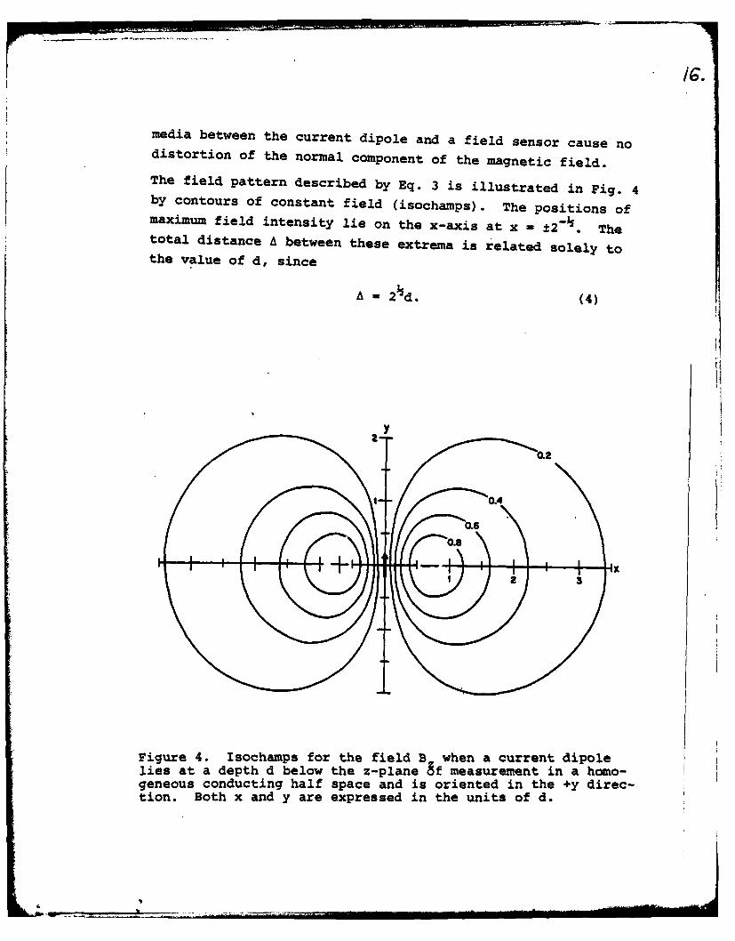
media between the current dipole and a field sensor cause nodistortion of the normal component of the magnetic field.

The field pattern described by Eq. 3 is illustrated in Fig. 4by contours of constant field (isochamps). The positions ofmaximum field intensity lie on the x-axis at x - ±2- . Thetotal distance a between these extreua is related solely tothe value of d, since

A = 2 d. (4)

Figure 4. Isochamps for the field B when a current dipolelies at a depth d below the z-plane of measurement in a homo-geneous conducting half space and is oriented in the +y direc-tion. Both x and y are expressed in the units of d.

71

The field at each extremum has the magnitude

U0 . (5)Bm = 0.385 4 "d2

Thus with a knowledge of 'd, obtained from a measurement of A,

together with a measurement of the maximum field Bm the magni-tude of Q can be deduced.

Although only the tangential component of 6 contributes to theexternal magnetic field, both tangential and normal componentscontribute to the electric potential at the surface of the halfspace. This potential is an expression of the volume currentthat spreads from the current dipole. The source of the volume

current can be imagined equivalently as being a charge dipoleof moment p = Ko0/a whose charge separation equals the lengthof the current dipole. Here K is the dielectric constant of

the medium, a is the conductivity of the medium, and eo is

the permittivity of free space. The volume currents flowingoutward from the positive charge and inward toward the nega-

tive charge match the impressed current of the dipole itself.

The resulting potential V at the surface can be deduced by

conventional arguments based on assuming an image dipole tosatisfy the boundary condition of no outward flow. If 6 is

inclined from the z-axis by an angle e' toward the +y-axis

we can express the contribution of the tangential componentof the dipole as

Q sine' y (6)VT 12ad2 (1 + x 2 + y2) 3/2

This has precisely the same form as Eq. 3 for B but the~zpattern is rotated by 900 about the z-axis. Moreover there

will be a contribution to the potential from the component

of the dipole that is normal to the surface:

Q cos9' 1 (7)N 2 ad2 (1 + X2 + y2) 3/2

The isopotentials shown in Fig. 5 vary in a complicated wayas the angle of inclination 6' is varied. One remarkable

feature is the dominant influence exerted by the end of thedipole which is closest to the surface. Moving from the

symmetrical tangential orientation of 6' = 90° by reducing6' by only 150 produces a factor of 2 difference between

the magnitudes of the potentials at the two extrema. A

reduction to 0' - 600 leaves only a hint of the weaker region.

Only a very careful and sensitive mapping of the isopotentials

could reveal the presence of a tangential component for

orientations e1<600. In principle surface potential measure-

ments could reveal both normal and tangential components;however in practice the normal component is emphasized,

unless the dipole is oriented to within a few tens of degreesof the tangential direction. In this sense the magnetic

measurements are complementary, since they detect only thetangential component.

Averaging by the Pickup Coil

A SQUID system provides an output signal that is proportional

to the total magnetic flux which threads its detection coil.For a magnetometer or a gradiometer having a sufficiently

long baseline this is the flux which passes through the pick-up coil. That is, the output is a measure of the averagefield B within the coil. In studies of the field pattern

from a current dipole it is important to know how faithfullyB(s) describes the actual spatial varation of the field B( ).One expects important distortions to appear if the

diameter "2a" of the pickup coil is so large that it iscomparable to the distance A separating the two field maximaon the surface of the skin. In the case where the situation

can be approximated by the conducting half space, which we

consider in this section, the measured value E given by theobserved variation of B would predict by Eq. 4 a much greater

value 3 of the dipole's depth than the actual depth d. And

o 90 Y O'= 750

0.2

0.4 0.2

06774i ( o.6

x

2,

G600 .o' o

-- 0

Figure 5. Isopotentials on the surface of a homogeneous con-ducting half space arising from the volume currents associatedwith a current dipole at a depth d and inclined from the +z-direction by an angle e' toward the +y-direction.

even if one knew this correct depth, using the measured valueof the field extremum m in Eq. 5 would lead to an incorrectmvalue Q for the dipole strength.

To evaluate how to correct for using a pickup coil of finite

size we have found it convenient to apply lead field theoryas developed by Baule and McFee (16,17) and Plonsey (18).

In this approach one assumes that there are two impressedsources: a current IRexp(jwt) that is passed through thepickup coil and a second current i(r)exp(jwt) that is the

impressed current density, both varying sinusoidally at a low

frequency w. From considerations of the field equationsdescribing the distribution of electric and magnetic fieldsPlonsey has obtained an expression that predicts the voltqge

that would be induced in the pickup coil if J r) were the

only source present. This expression contains informationabout the shape of the pickup coil in that it includes the

electric voltage L(r) that would be induced at each pointin space by the imagined flow of IR. EL(r) is called the

lead electric field. We generalize Plonsey's Eq. 20 toobtain an expression for the flux produced in the pickup coil,which is of more direct interest for SQUID systems than the

form of his equation:

= _E 'i(r') d3r'. (8)

Often Eq. 8 is written in terms of the ohmic current distri-bution that would be produced by the lead field: L( ) =

AL (r). Here L is known as the lead current. The lead

electric field is advanced in phase by n/2 with respect toIR ' since the field is caused by Faraday induction. Thus the

expression 9L/jw has the same phase as R, and we can no

longer be concerned with the phaser notation. If a positivevalue is obtained when evaluating the right hand side of

Eq. 8 for a given distribution of primary current, the net

flux produced in the pickup coil by this current has the same

sign as the flux produced within the coil by the imagined IR Because EL is proportional to IR the actual value chosen for

I is irrelevant for the calculation, and it could be taken

equal to unity.

A straightforward applicition of Eq. 8 involves many diffi-

culties, not the least of which is the fact that the variation

of electrical conductivity within the body must be taken

into account. Even for the homogeneous half space of interest

to us, a surface integral of the lead magnetic field must

first be solved in order to deduce L. Unfortunately,

expressions for the magnetic field pattern from even a cir-

cular pickup coil are complicated. It is much more convenient

to recast Eq. 8 into a form that depends on the lead vector

potential L produced by the flow of IR through the pick-

up coil: This potential is related to the lead magneticinduction by L = V x and to the lead electric field by

9 L- /L/at = -jWI. If the coil is oriented with its axis

perpendicular to the surface of the half space, no complica-tions arise from the effects of the surface. Then Eq. 8 can

be rewritten as1f- f (r (' d3 r'. (9)

R

This relationship is implicitly contained in lead field calcu-

lations reported by Malmivuo (19) for several configurations

of detection coils. This equation indicates that the orien-

tation for which a primary current density I i produces thegreatest flux 0 is along the direction of AL at its position.

If 3' is parallel to I, the flux is in the same direction as

that produced in the coil by the imagined IR' if antiparallel,

it is in the opposite direction.

To arrive at our goal of calculating the effect of a pickup

coil of finite size on the observed field pattern from a

current dipole, we integrate Eq. 9 when the dipole is located

at the position r:

R (10)

This remarkably simple expression is also particularly use-

ful. A detection coil with axial symmetry produces circularpatterns of AL about that axis. For example a circular loop

of radius "a" produces a vector potential directed circularly

in the same sense that IR flows around the coil. Its magni-

tude is given by (20)

AL(r) = 4o7r -1a(a2+r2+2ar.sin a)h (2-k2)K(k2)-2E(k

2)]0 k 2 "

where k2 = 4ar-sina (a2+r2 +2ar-sin a)-1 (11)

r = d(l+x2+y2)

sin a - (x2+Y2) d/r.

In these expressions "r" is the distance of the point of

interest from the center of the coil, and a is the angle be-

tween r and the coil's axis. K(k2) and E(k2)'are the complete

elliptic integrals of the first and second kind, such that

22in the limit of small "a" (or small k ) the expression in

square brackets reduces to rk2/16.

We now apply the expression in Eq. 10 to the case where the

coil is placed at the surface of the half space, and its cen-

ter lies at the position (x,y) in the z=0 plane. A current

dipole Q lies on the z-axis at z = -d and is oriented in the

+y direction. We choose to express our results in terms of

the averaged detected field as defined by

2B = /7ra2 . (12)z

Then Eq. 11 yields:

UoQ x 4d2 22B • 2 - (a2+r2+2ar sin a)-z (4rd (axy

2-k 2 )K(k 2) -2 E (k 2 (13)

In the limit of small "a" this expression reduces to that inEq. 3, so that Bz(x,y) is an exact representation of B,(x,y).But Eq. 13 is correct for any value of "a", and therefore itcan be used to assess the effect of measuring the field witha large pickup coil. For simplicity we consider the variation

of the measured field as the coil is moved along the x-axis(ymO), where it will pass through the most intense regionof field. Fig. 6 illustrates how for larger coils the maxi-mum observed value Bm is reduced and its position F/2 shiftsfurther away from the dipole's position.

From these results we have deduced correction factors that canbe used to adjust experimental results to compensate for useof a pickup coil of finite size. Fig. 7 provides a correc-tion factor d/d that can be applied to calculate the actualdepth "d", given the empirical value d = 1/2h from Eq. 4.The figure also gives the correction factor Q/Q for obtainingthe actual strength of the dipole given the empirical value

O= 4d 2Bm/0.385p o from Eq. 5. Note that in the expressionfor & the actual value of the dipole's depth appears and notthe empirical one. The corrections for depth and strengthare only on the order of 6% when the coil diameter 2a is halfof the observed separation A between field extrema. Butthe corrections escalate sharply when the diameter approaches

the value of A.

Current Dipole in a Sphere

When an element of neural current lies an appreciable distance

0.4 ,

a/d :0

0.3 a/d=0.5

a/da I

0.20

1C" - d/d / "

• =2

0.1

00 2 3

X (units of d)

Figure 6. Measured average field B for positions along the+x-direction when a current dipole fies at a depth d below thethe z-plane of measurement in a homogeneous conducting halfspace and is oriented in the +y-direction. The effect ofusing a pickup coil of finite diameter 2a is shown, as predic-ted by Eq. 13.

0

I.

0.8 -

Igo0.6

0.4- -

0.21-0 0.2 0.4 0.6 0.8 1.0

2a/ZFigure 7. Factors for obtaining the correct depth d andstrength Q of a current dipole in a half space from the valuesof d and Q deduced from measurements of the average fieldobtained with a pickup coil of finite size.

beneath the scalp we can expect the model of a current dipole

in a half space to be invalid. The curvature of the boundary

of the conducting medium becomes an important feature.

Consequently a better model might be a current dipole within

a conducting sphere. In this section we consider how features

of the observed field pattern can be applied to deduce the

depth and strength of a dipole. A comparison of these resultswith those of the preceding section will show when the in-

fluence of the curved boundary becomes important.

The demonstration by Baule and McFee (2) that a current dipoleproduces no external field in a situation of axial symmetry has

important consequences for the sphere model. It predicts forexample that a radially oriented dipole cannot be detected

magnetically, because the field from its volume current just

cancels the field from the dipole itself. Also significantis its prediction that a dipole at the center of the sphere

produces no external field. From continuity arguments we

expect that the field from a tangentially oriented dipole

will diminish toward indetectable levels as the dipole is

moved toward the center. Thus the magnetic technique will

not'directly detect deep-lying sources. Tripp (21) has shownthat if the shape of the boundary departs slightly from that

of a perfect sphere there is a correspondingly small changein the field pattern. In other words, predictions based

on the sphere model are not dramatically affected if there

are small departures from the ideal symmetrical boundary.

Grynszpan and Geselowitz (15) have deduced an expression forthe magnetic scalar potential outside a sphere when a tan-

gentially oriented current dipole is at a distance "b" fromits center. The result is independent of the radius R of

the sphere(if R>b). Thus R can denote instead the radial

distance to the point of interest where the field is measured,

with the sphere having a smaller radius. Concentric inhomo-

geneities either at shorter or longer radii than "b" do notalter the external field pattern (15). Therefore the head

can be modeled by concentric spherical shells of differing

but hovi'geneous conductivity to represent such features as

the cerebrospinal fluid, skull and scalp at radii exceeding

• .2

"b", and the field pattern outside remains undisturbed.

The situation will be described by a spherical coordinate

system as depicted in the inset of Fig. 8. We let 6 denotethe angle of declination toward the position of field measure-

ment, and o denote the azimuthal angle with respect to the

L.odepth of a current dipole

ZIG-.d

-0.8- bR

0.6-

0.4-0.2-

0.10.2-

0 t0 20 30

0 20 40 60 80 100 120 140 160 180angle between radial field extrema 8 (dog)

Figure 8. The depth d below the radius of measurement R forthe position of a current dipole in a conducting sphere asdetermined by the angular span 6 between the two positionsof most intense radial field BEr

x-axis. The "depth" of the dipole is d = R - b. From Eq. 30

of reference 15 we obtain an expression for the radial field:

bB oQ b coso sine

Br 2 r+ 2bR 3/2 (14)

41 L += (l-cos8)

This is equivalent to Eq. 22 of reference 22 which has beenderived by another method. The correspondence between this

expression and that written in Eq. 3 for the half space

model becomes apparent if we rewrite the latter as

UoQ L-- coso sineB 0 s (15)

Z ___T~* [+( R$ sin -217/2

where R' is the radial distance to the point in the z-plane

in which the field is measured. In the limit when the dipoleis at a shallow depth (d/R<<l and 6<<l) Eq. 14 becomes identi-cal to Eq. 15. In this limit the predictions of the sphere

model reduce to those of the half space model.

When mapping the component of a neuromagnetic field that is

normal to the scalp it is easiest to identify the regions

where the field is strongest. In the sphere model, Eq. 14

predicts that this occurs at a declination em where themagnitude of Br is maximum, as given by the solution to

d2 3 cosem2(R-d)R = 2 cose m 2

What the experimenter can directly measure is the total angular

spanS = 2e between the positions of maximum inward and maxi-m

mum outward field. The dipole lies on the radius midway be-tween these two positions. Its depth is given by the curvein Fig. 8 as determined by solutions to Eq. 16 for various

values for the total spin. Thus from a measurement of 6 , thedepth of the dipole below the radial distance of the pickup

coil can be deduced.

As the dapth increases and the dipole approaches the center of

the sphere, the angular span between field extrema tends toward1800. But as remarked earlier, the strength of the fielddiminishes toward zero in the limit d/R - 1, so it will be im-possible to detect central sources if the sphere model isapplicable. This effect.of the spherical boundary inweakening the maximum field through its effect on the volumecurrent is dramatically illustrated in Fig. 9. For the half

3.

strength of a current dipole

4rd'Bm0.385o

C

.2.5

20 40 60 80 100 120 140 160 180angle between radial field extreme, 8 (deg)

Figure 9. The strength Q of a current dipole in a conductingsphere as determined by the magnitude B of the most intenseradial field at either extremum at the fadius of measurementR, with the depth d of the dipole given by the curve in Fig. 8.

space, the maximum field Bm normal to the surface can beused to predict the strength of the current dipole as given

by Eq. 5. Were the same formula to be used for measurements

on a sphere with the maximum value of Br inserted in place ofBm, the deduced value denoted by 0hs underestimates the actual

strength of the dipole. Fig. 9 provides the correction factor

for how much stronger the actual Q is. For example, when the

angular span between extrema is 6 = 90° the dipole has an

actual strength that is twice the value of Qhs given by

Eq. 5. In making this calculation the value of the maximum

radial field and the actual value of "d" given by Fig. 8should be used. For a span of 6 = 1500 the actual strength

is 5 times greater than is given by Qhs calculated from Eq. 5.

In this section and the preceding one we have summarized

how the position and strength of a current dipole sourceare determined by the positions of the field extrema and

by the strength of the field at either extremum. Howeverthe human head is neither a sphere not a half space, and con-

sequently these results should be applied with caution. For

a specific application, an intercomparison of, the predictionsof the two models will provide some insight as to their

sensitivity to differing boundary conditions. But the

results do not give any hint of the possible importance of

non-concentric internal inhomogeneities within the brain andthe angular variation in skull thickness. The field pattern

from more complicated model sources involving multiple arrays

of current dipoles have been computed by Cuffin and Cohen (23).

They have also calculated the lead fields for several types

of magnetic detection coils and scalp electrode arrays, based

on a multiple concentric shell model for the head (24).

Evoked Fields

Magnetic fields which appear near the scalp in response to a

sensory stimulus have attracted considerable interest. Sensory

evoked brain responses, originating at the cortical level,

are believed to be among the simplest of neural signals and

therefore provide the best opportunity for gaining a foot-

hold on the functional organization of the brain. These

signals, however, are extremely weak ("4,00 fT) and in some

situations are masked by the ongoing spontaneous activity

of the brain. Therefore signal processing techniques have

been applied to average the responses to many identical

stimuli applied in sequence in order to bring. the signal of

interest above the noise. An "evoked response" in most cases

implies an "averaged evoked response."

Two types of stimuli may be used. The first is an intermit-

tently repeated stimulus where the effect of one stimulus hasenough time to disappear before the presentation of the next.

The response that is time-locked to each stimulus is called

the transient response. It is a complex wave which contains-positive and negative peaks, each of which may be charac-

terized by its delay (latency) following the stimulus. Thesecond type of stimulus is periodic and presented at a

repetition frequency so high that the effect of one stimulus

has not worn off before presentation of the next. Thisleads to the so-called steady state response (25). It is

represented by a response which is periodic at the frequency

of the stimulus or its harmonics and is characterized by theamplitudes and phases of its components. Usually only the

amplitude and phase of the response at the fundamental fre-

quency has been investigated in detail. The transition

between transient and steady state response is-believed to

occur for stimulus rates of N\4 Hz, depending on the type of

stimulus. The response of a linear system is completely de-

termined either by its transient response or a knowledge ofits steady state response at all stimulus frequencies. Human

sensory systems are not linear, and therefore it is not known

whether the two types of stimuli provide equivalent informa-

tion.

It is thought that activity evoked in the cortex of the brain

by a sensory stimulus produces the observed scalp potentialsand perhaps magnetic fields through the-polarization of large

numbers of cells. The cortex, which is only 1-3 mm thick, hasa cellular organization whereby pyramidal cell bodies arealigned transverse to the cortical layer with their long

apical dendrites extending outward toward the surface. Adendrite when depolarized as a consequence of synaptic activity

may establish a graded potential until the threshold for theaction potential is surpassed. In this condition the altered

conductivity of the cell membrane sets up an extracellular

current that flows toward the dendrite, which acts as a "sink"for the current. The cell body, a "source," remains electric-

ally positiveand the dendrite relatively negative. The colum-

nar organization within the cortex thus may support a currenttransverse to the cortical surface in regions where pyramidal

cells are excited that produces an external magnetic field.Other neural elements such as stellate cells probably do notcontribute to net current densities owing to their random

orientations.

If this polarization current is indeed the origin of the

evoked magnetic field, the convolutions of the cortex pre-sent a complicated geometry which should have an importantinfluence on the observed field patterns. Fig. 10 shows

that three of the most accessible sensory areas lie near orwithin deep fissures of the cortex, where currents lie tan-

gential to the scalp. Thus from considerations mentioned

earlier concerning the magnetic field from a current dipole

and its volume current in either a half space or sphere weshould expect neural activity near these fissures to be

emphasized in the patterns of evoked field. Some recentanalyses of evoked scalp potentials have taken into account

the topology of these fissures when dealing with sources

that are believed to lie within their depth (see for example

reference 26).-,,WN

I

Longitudinal fissure motor co Rolandic fissure

Frontal lobe Central lobe

Somatosensory cortex

Parietal lobe

Occipital lobe

Sylvian fissure v cViua cortex

Temporal lobe

Auditory cortex

Figure 10. Surface of the brain showing its principal fissuresand sensory projection areas of the cortex.

Visually Evoked Field

The first observations of magnetic responses were achieved

with visual stimuli. The subject observed either brief

flashes of light or a pattern of changing luminance presented

on the face of an oscilloscope (27-29). One interesting

finding in the steady state visually evoked field (VEF) re-

ported in the initial study of Brenner et al. (28) is a shar-

per localizability over the occipital area near the visual

cortex as compared with the visually evoked potential (VEP),

which can be observed as far as frontal areas of the head.

Subsequent investigations of transient VEFs by Zimmerman

et al. (30) in which magnetic and potential responses were

directly compared on the same subjects showed that the VEP

extended into posterior parietal and temporal areas but

nevertheless was significantly more confin~d than the VEP.

The temporal features of the VEF have revealed important

evidence concerning the functional organization of the visual

system in humans. Williamson et al. (31) found that the

latency of the steady state response varies with features

of the stimulus pattern. The stimulus was a grating pattern

formed by a sinusoidal variation of the luminance across the

face of an oscilloscope. It was presented in the "contrast

reversal" mode whereby the grating is periodically shifted

sideways by half a spatial wavelength, thereby causing regions

of higher luminance to be replaced by regions of lower

luminance. As the overall average luminance remains

unchanged, the stimulus is simply one of a changing pattern

and is characterized by the spatial frequency of the grating.

The latency of the neuromagnetic response was found to

increase from n'80 ms; for a gratiztg of low spatial frequency

(about 1 cycle of luminance variation encompassed within 1

degree of visual angle) to more than %,120 ms for a high

spatial frequency (about 5 cycles/degree). This observation

appears significant because a similar variation was reported

by Breitmeyer (32) for the reaction times of subjects when

suddenly presented by the same types of gratings of various

spatial frequencies. The reaction times being consistently

115 ms longer than the neuromagnetic latencies, it is natural

to associate the 115 ms with the motor response time that

follows activity in the visual cortex. The latency thus

represents the sensory response time and appears to be a

significant measure of physiological activity.

Visual stimuli are particularly useful for studies of sensory

processes because both pattern and presentation rate can be

varied separately. For instance, the dependence of the neuro-magnetic latency on spatial frequency is found to disappearif the stimulus presentation rate is sufficiently rapid (33).

This behavior provides the first physiological evidence fortuned transient and sustaining channels in the human visualsystem as suggested by psychophysical and animal studies.Additional results of this type of study are presented byBrenner et al. in these Proceedings (34).

Here we shall concentrate on the information that can beobtained about the locations of the sources of the evokedfield. In carrying out measurements of evoked fields in our

laboratory we have found an advantage in choosing stimuli

that evoke a response of the simplest type possible. Thismeans reducing features of the stimulus to the minimum num-

ber of variables. Once these responses are understood itwould make sense to use more sophisticated stimuli. For

example, the field pattern over the visual cortex is compli-cated partly because it is the superposition of effects fromsources in both hemispheres of the brain (35). It becomessimpler if activity in only one hemisphere at.a time is

evoked. This can be accomplished by presenting the visualstimulus in only the left half visual field or the right halffield. The image thus appears on the opposite half of the

retinas, and by the nature of the neural connections corticalactivity appears only in the opposite hemisphere. The lowertwo maps in Fig. 11 illustrate the observed steady state

amplitudes for the VEF (34) when one hemisphere at a timeresponds. The field leaves the head from one of the indi-

cated regions and enters the other. The stimulus was agrating having a spatial frequency of 5 cycles/degree whose

contrast was reversed at 13 Hz. The contrast was 33%,

average luminance was 52 cd/m , and the full field displaywas a circular region encompassed by a visual angle of 9° .

The format for the field maps in Fig. 11 is based on a spheremodel for the head, with a globe-like coordinate system. The

:3G,

RHF LHF

VEPO, JPA

(Dorcey of al.)

92 mscomponent

VEF

steadystate

Figure 11. Visually evoked transient potential (upper figures)adapted from Fig. 78 of reference 37 and visually evokedsteady state field (lower figures) from reference 34 for halfvisual field stimulation. The stipled area for the VEPrepresents negative potentials. Isopotential contours aredrawn for equal increments in potential. Isochamps represent100, 200, 300, and 400 fT amplitudes.

"north" and "south" poles lie near the ears, and the equator

Ti'ds with the midline. The meridian passes over the

inion, which is the slight bump at the base of the skullwhere muscles attach, and angles are measured with respect

to this landmark. The inion is portrayed as the center of

each sphere in Fig. 11, and grid points are at intervals of

150 (approximately 2.5 cm distances on the adult head). We

chose this format because it was used in the recent work of

Darcey et al. (36) who obtained detailed maps of evoked

potential distributions by half field stimuli. Consequentlywe have the opportunity to make a direct comparison of the

information provided by the two measures. Darcey et al.

obtained transient responses with an array of 40 electrodes

placed at the grid points over the posterior region of the

scalp. The reference potential was the average potential

from all electrodes (37). The stimulus was a red checkerboard

pattern of 18 min arc checksize (about 1.5 cycles/degree

spatial frequency), with 95% contrast, 68 cd/m2 average lumi-nance, and 30 ms display time presented in Maxwellian view

at infinity to one eye. When the checkerboard was not presen-

ted, the 10 degree circular full field viewing screen provideda uniform luminance which matched the average luminance of

the checkerboard. Thus in both the VEP and VEF the stimulus

was a change in pattern, not luminance.

The first component of the transient VEP measured with a 30 Hz

bandwidth was reported to have the same latency of 92 ± 4 ms

for each of three subjects. The locations of potentialextrema and the equipotential patterns remained approximately

the same for a period of 20 to 30 ms during which the ampli-

tude rises, reaches its maximum and then decays. The maps

for one subject are reproduced in the upper half of Fig. 11

(36). The latency of the VEP is comparable to the latency

of the steady state VEF shown in the lower half. Although

these responses are for different subjects, there may be

some value in comparing them.

For both VEP and VEF the strongest effects are seen over the

hemisphere that is contralateral to the half of the visualfield presenting the stimulus. The polarity of the magnetic

field and of the scalp potential suggest a current dipole

source. However the VEP -is considerably more widespread

than the VEF, in agreement with earlier reports (28). Posi-tive extrema in the potentials are found '\450 or more from

the midline whereas the field extrema are only -10° . Thusvolume currents flow through the greater portion of the brain

and scalp, but the magnetic field remains fairly well

localized near the visual cortex suggesting that they are dueto the high-density currents in the immediate vicinity of

the active neurons.

Nevertheless Darcey et al. (36) have shown that an assumed

dipole source for the potential can accurately predict the

pattern. Using a multiple spherical shell model for the

head they calculated the position and orientation of thedipole that would give a pattern of equipotentials that best

agree with their observations. The predicted depth depends

in general on the relative shell radii that are assumed,

which can vary substantially among individuals. For illus-trative purposes, Darcy et al. chose nominal values, whereby

the inner and outer radii of the skull are 90% and 98% of

the radius of the scalp. Table 1 summarizes the coordinates

for this source as read from the figures in their paper.

For comparison we have deduced the location of an equivalent

current dipole which would account for the positions of theextrema in the magnetic field. To obtain the depth we first

assumed a half space model, and taking the measured distance

X between extrema deduced the value of "Z" from Eq. 4. Then

we obtained the actual depth "d" by using the correction

factor in Fig. 7 appropriate for the 2.4 cm diameter of the

pickup coil. This was at most a 15% decrease between "i"

and "d". Finally 0.8 cm was subtracted from the value of "d"

to account for the distance between the pickup coil and scalp.

The remaining depth for the source below the scalp is tabu-

lated in Table 1. Vertical and lateral positions were deter-

mined directly by the position cf the midpoint between the

field extrema, projected toward the center of the head by

a distance equal to the depth of the dipole.

As a second estimate for the source location we took the

sphere model with a radius of 10.8 cm to the position of the-

pickup coil. From the measured angle 6 between field extrema

we deduced the depth of the current dipole by using the

curve in Fig. 8. From this value of "d" we subtracted 0.8 cm

to obtain the radial depth below the scalp. The corresponding

positions listed in Table 1 for the sources in the two

hemispheres do not differ substantially from those deduced

by assuming the half space model. Therefore the analysis

of the magnetic data to this degree of precision is not

sensitive to the assumed shape of the head.

The positions indicated in Table 1 show fair agreement between

the VEP and VEF for lateral source coordinates that primarily

depend on symmetry features of the maps shown.in Fig..11.

Vertical and horizontal positions of the sources lie close

to the midline and several centimeters above the inion. The

VEF indicates that the left and right hemisphere sources lie

somewhat closer together than the sources deduced from the

VEP, and in that sense correspond more closely to polariza-

tion currents within the cortex at either side of the longi-

tudinal fissure. One outstanding difference between the

deduced positions is in the predicted depths of the sources.

The VEP predicts a depth below the scalp of 5 cm, whereas

the VEF predicts 2 cm. These correspond approximately to

4 cm. and 1 cm depths below the surface of the brain when

the thickness of the scalp and skull are subtracted. It is

informative to compare these predictions with anatomical

features of the cortex and its dimensions. A portion of the

cortex may be exposed at the occipital pole as illustrated

in Fig. 10, but most of its area is found at inner surfaces

Table 1

Location of the current dipole in each hemisphere that bestaccounts for the observed VEP and VEF mapped in Fig. 11.Vertical and lateral coordinates lie in the plane perpendi-cular to the radius vector from the center of the head tothe inion.

RadialDepth

Vertical Lateral BelowStimulus Position Position Scalp

VEP (reference 36)0: JPA RHF + 2.0 - 2.5 +5.5±1 cm

LHF 2.3 + 2.0 5.0±0.3

VEF half space model RHF 3.3 - 1.7 1.6

0: RL LHF -2.0 + 0.7 3.2

sphere model RHF 3.4 - 1.7 1.3

LEF 2.2 + 0.7 2.5

of each hemisphere within the longitudinal fissure, with

extensions into each hemisphere along the surface of the

calcarine fissures which meet the longitudinal fissure at

nearly right angles. Anatomical studies of 52 hemispherescollected at autopsy show that the cortex extends inward from

the occipital pole to a depth of typically 5 cm (38). Basedon studies of the visual effects of war wounds in the cortex,

the first centimeter of depth appears devoted to projections

of information from the central ,0° of the visual field,

with more peripheral regions being represented at successively

greater depths. Consequently, the depth of the current dipole

source deduced from the VEF appears in good agreement withthis functional arrangement, since the stimulus included only

the central 90 of the visual field. By contrast, the VEP

locates the source at a much greater depth, even though peri-

pheral regions of the visual field also were not stimulated.

The reason for this difference is yet to be understood. It is

possible that activity in the cortex is evoked at a much

greater depth than previously believed, and the rapid de-crease in magnetic field strength with distance from the

source favors the closer lying regions in the VEF. If thisis true then the VEP and VEF characterize activity in

differing regions of the cortex, with the VEP emphasizing theperipheral field. However, this cannot be the case since it

is known that foveal stimulation is the major contributerto the VEP. On the other hand, if only the most posteriorregions of the visual cortex are active, the volume currents

associated with this source evidently become much more wide-spread at the scalp than is predicted by concentric spherical

shell models for the head. The equipotentials appear to

be considerably broadened compared with the isochamps thanis predicted by lead field calculations for a current dipole

(24). A pattern that is anomalously expanded when interpre-ted with a concentric spherical shell model would imply asource position that is anomalously deep.

It is evident from the VEF shown in Fig. 11 that the current

dipole assumed to represent the source in each hemisphere

may be tipped at different angles with respect to the mid-line. Most often they are found to be nearly horizontal,but it is not unexpected to find intersubject differencesowing to different placement of the cortex and calcarinefissures in the two hemispheres. Tipping of the source

dipoles was also revealed by the analysis of the VEP repor-

ted by Darcey et al. (36,37). The angle may vary considerablyfrom one subject to another and between the two hemispheresin the same subject. The potential studies also reveal a

feature that has not yet been extracted from the magneticdata: in some cases the dipole is also tipped slightly for-wards or backwards. This indicates the presence of a smallradial component of the dipole that for the half space orsphere models would not produce an external magnetic field.

Somatically Evoked Response

The somatosensory cortex which responds to stimuli applied

to the body is found at quite a different region of the

brain than the visual cortex (see Fig. 10). Studies of

somatically evoked neural activity can exploit the advantage

that responses to stimulation of various regions of the skin

project to different areas of the cortex. The map of the

projection areas was determined by electrical Ueasurements

during neurosurgical operations when portions of the skull

above the cortex are removed (39). The first observation

of the somatically evoked magnetic field (SEF) by Brenner

et Al. (40) demonstrated rather sharp localizability of the

underlying source, which was found to be near the expectedarea of the cortex. A repetitive electrical stimulus applied

to the little finger produced a steady state evoked fieldwhose center of symmetry could be determined with a precision

of better than 1 cm. It was found over the expected position

of the Rolandic fissure in the hemisphere contralateral tothe side being stimulated. A current dipole source at this

position would be perpendicular to the fissure to account for

the field pattern. When instead the thumb was stimulated,she pattern shifted along the fissure toward the ear by 2 cm,

in correspondence with the positions of the respective projec-

tion areas of the cortex (39). The latency of the neuromag-netic response was typically 70 ms for five subjects. No

equivalently sharp localizability has been obtained from

somatically evoked scalp potentials (SEP). In fact, studies

of the transient SEP by Goff et al. (41) show that except

for the earliest components 20-30 ms following stimulation

potential variations are found on both sides of the head.

Recently in our laboratory it has become possible to observe

the transient SEF, and direct comparisons of the components

of the SEP and SEP have been made (42). The details of some

of these studies are reported by Okada et al. (43).

We can apply the analysis developed earlier in this paper

to deduce the position of the current dipole that could give

rise to the observed field. For the pattern reported in

reference 40 for a stimulus to the little finger the field

extrema are separated by A-4 cm. Since the pickup coil

has a diameter of 2a - 2.4 cm, Eq. 4 predicts an empiricalvalue of =2.8 cm for the depth of the dipole. Assuming

the half space model for the head permits us to use thecorrection factor in Fig. 7 for the finite size of the pickupcoil and deduce an actual depth of d - 2.4 cm. Subtractingfrom this the distance 0.8 cm between the pickup coil andscalp leaves 1.6 cm for the depth of the dipole below thescalp. For a thickness of "%41 cm for the scalp and skullwe conclude that the source lies within 1 cm of the innersurface of the skull. This value is entirely reasonable ifthe source represents depolarization currents transverse tothe cortex in the primary projection area, where it formsthe posterior bank of the Rolandic fissure. For such anear-l.ying source we can expect that the half space modelfor the head may be a reasonable approximation when analyzingmagnetic effects.

Auditory Evoked Fields

Magnetic fields evoked by auditory stimuli may provide anotherexample of good localizability of cortical activity. A tran-

sient evoked field following a click stimulus was discovered

by Reite et al. (44) in the region of the Sylvian fissure.

Components with latencies in the range of 43-48 ms and 98-118

of opposite field polarity were observed' within a localized

region of a few centimeters extent; but a corresponding second

region of intense field was not reported in their publication,leaving in doubt the exact location of the current source.

Farrell et al. (45) were able to obtain substantially lower

background noise in their remote laboratory and identified

two regions of intense field with opposite field directions.

One was close to the left temple (two thirds of the dis-

tance from EEG position F 7 to F 3) and the other above the

left ear (1 cm anterior to the point centered between T 3 and

C 3) on the left side of the head. They identified a component

having a latency of 50 ms with a positive component of the

AEP having a similar latency but showing a maximum amplitude

near the top of the head. Because the amplitude of this

component in the AEF decreases rather slowly as the pickup

coil is moved further from the scalp they argued that itrises from a source lying much deeper than the surface cortex

of the brain. Farrell et al. suggested that a source model

that would be consistent with the polarities of both the

AEF and AEP is a pair of current dipoles lying deep within

the temporal lobe, symmuetrically placed on both sides of the

longitudinal fissure and directed upward.

By contrast with this localization, the auditory evoked

potential (AEP) is widespread over the scalp, and no com-

ponents appear to be localized specifically over the auditory

cortex (41). One topic of discussion in the evoked potential

literature concerns the problem of finding an "indifferent"

location for the reference electrode so as to obtain voltages

that are independent'of the reference location. Changes in

the reference potential may bias the interpretation of poten-

tial measurements taken from only a few positions, as has

been discussed with regard to the AEP in references 46-48.

This problem of seeking an indifferent location is completely

avoided in magnetic studies. Nor does the problem seem to

introduce uncertainty for the interpretation of evoked poten-

tials obtained by a large array of electrodes, where only the

potential differences across the scalp are the basis for sub-

sequent analysis.

more recent magnetic studies by Brenner et al. (35) of the

steady state AEP to click stimuli presented at 36 Hz have

provided quantitative data from which the actual depth of thesource can be estimated. As remarked by Reite et al. (44) andFarrell et al. (45) the response amplitude is considerably

weaker than for the VEF and SEF, which may be due in part tothe greater distance of the source from the pickup coil.

Only fields near the two extrema could be resolved. The cen-ter of the pattern lies over the Sylvian fissure in agreement

with the studies cited above. If attributed to a current

dipole, the dipole would be directed perpendicular to thefissure. The latency of responses measured for stimulus

rates between 27 and 45 Hz was 46 1 1 ms for one subject, andcomparable values were obtained for two other subjects. Thefield directions on the two sides of the head are the reverse

of each other as is consistent with symmetric current flow

in the two hemispheres.

Taking, the observed separation of A - 7 cm between extrema, wededuce from the half space model that the depth below the scalp

of the current dipole in each hemisphere is 4 cm. By compari-son the sphere model predicts a depth of 3.2 cm. The differ-

ence is negligible considering the present accuracy of the data.The predicted depth is sufficiently shallow to represent

activity in the portion of the auditory cortex lying within

Heschl's gyri,. in agreement with reference 45. This extension

of the Sylvian fissure is essentially transverse and could thussupport depolarization currents in the direction which the cur-

rent dipole represents. Vaughan and Ritter (46) had suggested

that this is the source for a late (200 ms) component of theAEP whose polarity was observed to reverse across the Sylvianfissure, when the nose is the reference position for measuring

potentials.

Recently Aittoniemi et al. (49) and Hari et al. (50) reportedmeasurements of quite a different type that provide evidence

for evoked activity in the auditory cortex. Magnetic res-

ponses were observed during the presentation of a sustained

auditory stimulus consisting of a tone at 1 kHz maintained

for 900 ma. They found components of the AEF with latencies

of 100 and 180 ms following the onset of the tone that agreed

closely in time with components of the AEP. In addition a

sustained field extending for the duration of the tone was

seen in both records. Amplitude extrema with opposing field

directions were found near the estimated ends of the Sylvian

fissure and a tangential component of the field connecting

them was observed. The variation of the field amplitude with

position over the scalp was more pronounced than in the elec-

trical response. From the field pattern and the observed rate

at which the field amplitude decreases as the pickup coil is

moved away from the scalp Hari et al. concluded that the

source lies in the auditory cortex, and not in frontocentral

cortical areas as suggested by the location of the strongest

AEP (51). Here once again the pattern of evoked field permits

a localization of the neurall'source that the scalp-recorded

potentials had not resolved.

Summary

The observed patterns of magnetic field evoked by visual,

somatic, and auditory stimuli can be analyzed in first ap-

proximation as though arising from current dipole sources.

The location of the dipole in each case so far considered is

found to lie within the primary projection area of cortical

activity for the respective stimulus modality. It is rela-

tively shallow in the case of somatic and visual stimuli, and

is considerably deeper for auditory stimuli. The predicted

depths are insensitive as to whether the head is approximated

as a conducting half space of infinite extent or as a conduc-

ting sphere. This is because the observed field patterns are

rather sharply localized near their current sources. By

contrast the observed evoked potentials reported in the

literature are considerably more widespread.

Temporal features of the evoked fields appear physiologically

significant. The latencies for steady state responses are

S17.

typically 80 ms for patterned visual stimuli of low frequency,

70 ms for somatic stimuli produced by a short current pulse,and 46 ms for auditory click stimuli. Reaction times for

visual stimuli of various spatial frequencies vary in the

same way as the neuromagnetic latencies as the spatialfrequency of the pattern is increased. The difference of

115 ms between the two measures has been attributed to themotor response time, which in a serial model is added to

the sensory response time to make up the total reaction time(31). Reaction times to a somatic stimulus when reduced bythe value of the latency predict a motor response time of105 ms (40). Reaction times to a click auditory stimulusobtained by Brenner in our laboratory when reduced by

the neuromagnetic latency yield a motor response time of

110 ms. Thus the deduced motor response times are virtuallyidentical across stimulus modalities. This feature lends

support to the serial processing model and indicates that

steady state magnetic responses designate a physiologicallysignificant time in the sequence of the brain's response to

a sensory stimulus.

This brief account shows that during the past 5 years since

the discovery of the sensory evoked magnetic field, sufficientprogress has been made to demonstrate some of the unique ad-

vantages of neuromagnetic techniques for studies of the brain.

New and significant results are being obtained at an ever

increasing rate. This approach to investigating cortical ac-tivity is an important complement of the psychophysical mea-

sures of human perception and single cell recordings in ani-mals. It should play an important role in resolving many of

the ambiguities that presently exist for interpretations ofevoked scalp potentials as well.

We wish to acknowledge our informative discussions with many

colleagues; particularly D. Brenner, T. Darcy, E. Maclin and

Y. Okada. We are also grateful to T. Darcy, J. Ary, and

D.H. Fender for permission to cite their evoked potential data

before publication.

References

Supported by the Office of Naval Research Contract N00014-76-C-0568 and by the National Institutes of Health Grants1 ROI EY02059-02 and 1 RO AM26654-011:.

t Fulbright Senior Research Scholar at the Service dePhysique des Solides, Universitd de Paris XI, 1979-1980.

1. Williamson, S.J., Kaufman, L.: Crit. Rev. in Bioengineer-ing, in preparation.

2. Williamson, S.J., Kaufman, L.: J. Magn. Magn. Mat.,submitted.

3. Williamson, S.J., Kaufman, L., Brenner, D.: in Supercon-ductor Applications: SQUIDS and Machines, Schwartz, B.B.,Foner, S., Eds., Plenum Publishing, New York, 1977, p. 355.

4. Reite, M., Zimmerman, J.E.: Ann. Rev. Biophys. Bioeng. 7,167 (1978).

5. Woodworth, R.S.: Experimental Psychology, Henry Holt andCo., New York, 1938.

6. Kaufman, L.: Perception: The World Transformed, OxfordUniversity Press, New York, 1979.

7. Jeffreys, D.: in Visually Evoked Potentials in Man: NewDevelopments, Desmedt, Ed., Oxford University Press, NewYork, 1978.

8. Cohen, D.: Science 161, 784 (1968).

9. Cohen, D.: Science 175, 664 (1972).

10. Reite, M., Zimmerman, J.E., Edrich, J., Zimmerman, J.:Electroenceph. Clin. Neurophysiol. 40, 59 (1976).

11. Hughes, J.R., Hendrix, D.E., Cohen, J., Duffy, F.H.,Mayman, C.I., Scholl, M.L., Cuffin, B.N.: Electroenceph.Clin. Neurophysiol. 40, 261 (1976).

12. Hughes, J.R., Cohen, J., Mayman, C.I., Scholl, M.L.,Hendrix, D.E.: J. Neurol. 217, 79 (1977).

13. Bleaney, B.I., Bleaney, B.: Electricity and Magnetism,3rd Edition, Oxford University Press, Oxford, 1976.

14. Cohen, D., Hosaka, H.: J. Electrocardiology 9, 409 (1976).

15. Grynszpan, F., Geselowitz, D.B.: Biophys. J. 13, 911(1973).

16. Baule, G.M., McFee, R.: J. Appl. Phys. 36, 2066 (1965).

17. Baule, G.M.: in Advances in Cardiology, Vol. 10, Rush, S.,Lepeschkin, E., Eds., S. Karger, Basel, 1974, P. 304.

'

18. Plonsey, R.: IEEE Trans. Biomed. Eng. BME-19, 239 (1972).

19. Malmivuo, J.: Acta Polytechnica Scadinavica, ElectricalEngineering Series, No. 39, Helsinki, The Finnish Academyof Technical Services, 1976.

20. Jackson, J.D.: Classical Electrodynamics, John Wiley andCo., New York, 1962, p. 142.

21. Tripp, J.H.: in Cardiovascular Physics, Vol. 1, Ghista,D.N., Van Vollenhoven, E., Yang, W., Eds., Karger, Basel,1979, P. 29.

22. Cuffin, B.N., Cohen, D.: IEEE Trans. Biomed. Eng. BME-24,372 (1977).

23. Cuffin, B.N., Cohen, D.: J. Appl. Phys. 48, 3971 (1977).24. Cuffin, B.N., Cohen, D.: Electroenceph. Clin. Neuro-

physiol. 47, 132 (1979).

25. Regan, D.: Evoked Potentials in Psychology, Sensory Phy-siology, and Clinical Medicine, Chapman and Hall, London,1971.

26. Goff, W.R., Allison, T., Vaughan, H.E., Jr.: in EventRelated Potentials in Man, Callaway, E., Koslow, S.H.,Eds., Academic Press, New York, 1980, in press.

27. Cohen, D.: IEEE Trans. 'Magn., MAG-ll, 694 (1975).

28. Brenner, D., Williamson, S.J., Kaufman, L.: Science 190,480 (1975).

29. Teyler, T.J., Cuffin, B.N., Cohen, D.: Life Sciences 17,683 (1975).

30. Zimmerman, J., Edrich, J., Zimmerman, J.E., Reite, M.: inProc. San Diego Biomedical Symposium, Vol. 17, Martin,J.I., Calvert, E.A., Eds., Academic Press, New York, 1978,p. 217.

31. Williamson, S.J., Kaufman, L., Brenner, D.: Vision Res. 18,107 (1978).

32. Breitmeyer, B.G.: Vision Res. 15, 1411 (1975).

33. Williamson, S.J., Kaufman, L., Brenner, D.: J. Appl. Phys.50, 2418 (1979).

34. Brenner, D., Okada, Y., Maclin, E., Williamson, S.J.,Kaufman, L.: this volume.

35. Brenner, D., Williamson, S.J., Kaufman, L.: submitted forpublication.

36. Darcey, T., Ary, J.P., Fender, D.H.: submitted forpublication.

37. Darcey, T.: Ph.D. Thesis, California Institute of Tech-nology, 1979, unpublished.

38. Stensaas, S.S., Eddington, D.K., Dobelle, W.H.: J. Neuro-surg. 4, 747 (1974).

39. Pennfield, W., Rasmussen, T.: The Cerebral Cortex of Man,Macmillan, New York, 1950.

40. Brenner, D., Lipton, J., Kaufman, L., Williamson, S.J.:Science 199, 81 (1978).

41. Goff, G.D., Matsumiya, Y., Allison, T., Goff, W.R.:Electroenceph. Clin. Neurophysiol. 42, 57 (1977).

42. Kaufman, L., Okada, Y., Brenner, D., Williamson, S.J.:submitted for publication.

43. Okada, Y.C., Kaufman, L., Brenner, D., Williamson, S.J.:this volume.

44. Reite, M., Edrich, J., Zimmerman, J.T., Zimmerman, J.E.:Electroenceph. Clin. Neurophysiol. 45, 114 (1978).

45. Farrell, D.E., Tripp, J.H., Norgren, R., Teyler, T.J.:Electroenceph. Clin. Neurophysiol., in press; and thisvolume.

46. Vaughan, H.G., Jr., Ritter, W.: Electroenceph. Clin.Neurophysiol. 28, 360 (1970).

47. Picton, T.W., Hillyard, S.A., Krausz, R.I., Galambos, R.:Electroenceph. Clin. Neurophysiol. 36, 179 (1974).

48. Peronnet, F., Michel, F., Echallier, J.F., Girod, J.:Electroenceph. Clin. Neurophysiol. 37, 225 (1974).

49. Aittoniemi, K., Hari, R., Kuusela, M.-L., Katila, T.,Varpula, T.: in Proc. of the Third National Meeting inBiophysics and Medical Engineering in Finland, Lappeen-ranta, 1979, Ch. A7.

50. Hari, R.; Aittoniemi, K., JArvinen, M.-L., Katila, T.,Varpula, T.: Technical Report TKK-F-A399, Department ofTechnical Physics, Helsinki University of Technology, 1979;and this volume.

51. Picton, T., Woods, D., Stuss, D., Campbell, K.: in Multi-disciplinary Perspectives in Event-Related Brain PotentialResearch, Otto, D., Ed., U.S. Government, Washington, D.C.,1978, p. 515.

.. .rr.',, " - . ... "'" .. ........ . . .. ' ... f

'I