lab unit 3: force spectroscopy...

LAB UNIT 3 Force Spectroscopy Analysis

2009LaboratoryProgram 55

LAB UNIT 3: Force Spectroscopy Analysis Specific Assignment: Adhesion forces in humid environment Objective This lab unit introduces a scanning force microscopy (SFM) based

force displacement (FD) technique, FD analysis, to study local adhesion, elastic properties, and force interactions between materials.

Outcome Learn about the basic principles of force spectroscopy and receive

a theoretical introduction to short range non-covalent surface interactions. Conduct SFM force spectroscopy measurements as a function of relative humidity involving hydrophilic surfaces.

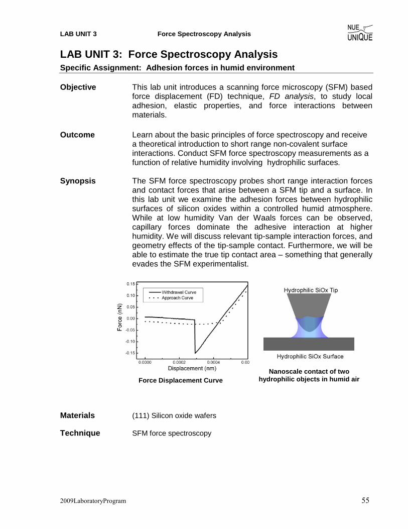
Synopsis The SFM force spectroscopy probes short range interaction forces

and contact forces that arise between a SFM tip and a surface. In this lab unit we examine the adhesion forces between hydrophilic surfaces of silicon oxides within a controlled humid atmosphere. While at low humidity Van der Waals forces can be observed, capillary forces dominate the adhesive interaction at higher humidity. We will discuss relevant tip-sample interaction forces, and geometry effects of the tip-sample contact. Furthermore, we will be able to estimate the true tip contact area – something that generally evades the SFM experimentalist.

Force Displacement Curve

Nanoscale contact of two hydrophilic objects in humid air

Materials (111) Silicon oxide wafers Technique SFM force spectroscopy



Table of Contents 1. Assignment................................................................................................... 57 2. Quiz – Preparation for the Experiment....................................................... 58

Theoretical Questions................................................................................................ 58 Prelab Quiz ................................................................................................................ 58

3. Experimental Assignment ........................................................................... 60 Goal ........................................................................................................................... 60 Safety......................................................................................................................... 61 Instrumental Setup..................................................................................................... 61 Materials.................................................................................................................... 61 Experimental Procedure ............................................................................................ 61

4. Background: Non-Covalent Short Range Interactions ................................. and Capillary Forces................................................................................ 67

Motivation ................................................................................................................. 67 Short Range Interactions and Surface Forces............................................................ 67 Van der Waals Interactions for Point Interactions .................................................... 69 Surface Forces ........................................................................................................... 69 Hamaker Constant ..................................................................................................... 71 Van der Waals Retardation Effects ........................................................................... 72 Adhesion and Surface Energies................................................................................. 72 Cutoff Distance for Van der Waals Calculations ...................................................... 73 Capillary Forces due to Vapor Condensation ........................................................... 74 Critical Humidity for Capillary Neck Formation ...................................................... 75 Estimation of the Tip Radius Utilizing the Capillary Effects ................................... 76 Modification of Hydrophobicity (Wettability).......................................................... 78 Force Displacement Curves ...................................................................................... 79 References ................................................................................................................. 80 Recommended Reading............................................................................................. 80

5. Appendix....................................................................................................... 81 Tool for Sigmoidal Data Fit ...................................................................................... 81 Tool for Hamaker Constant Calculation (provided in Excel Toolbox)..................... 81



1. Assignment The assignment is to experimentally determine the effect of humidity on adhesion forces for hydrophilic surfaces and to employ the theories and background information to discuss the experimental results. The steps are outlined here:

1. Familiarize yourself with the background information provided in Section 4. 2. Test your background knowledge with the provided Quiz in Section 2. 3. Conduct the adhesion-humidity experiments in Section 3. Follow the step-by-step

experimental procedure. 4. Analyze your data as described in Section 3 5. Finally, provide a report with the following information:

(i) Results section: In this section you show your data and discuss instrumental details (i.e., limitations) and the quality of your data (error analysis).

(ii) Discussion section: In this section you discuss and analyze your data in the light of the provided background information.

It is also appropriate to discuss sections (i) and (ii) together. (iii) Summary: Here you summarize your findings and provide comments on how your

results would affect any future AFM work you may do. The report is evaluated based on the quality of the discussion and the integration of your experimental data and the provided theory. You are encouraged to discuss results that are unexpected. It is important to include discussions on the causes for discrepancies and inconsistencies in the data.



Dielectric Constant

Refractive Index

SiOx 3.78 1.45Si 12 3.45Air 1 1

2. Quiz – Preparation for the Experiment Theoretical Questions (1) Given the data below, plot the Lennard Jones potential for N2-N2 interaction and Ar-Ar

interaction for distances between 0.25 and 1.4 nm. (Hint: assume point-point interaction, use Excel and make the calculation increment 0.01 nm for greatest clarity. Also select a y-axis range from -0.05 to 0.05 eV).

Molecule ε (eV) σ (nm) Ar 0.01069 0.342 N2 0.02818 0.368

(2) Provide a detailed description (with sketch) of an attractive FD curve. Under what condition

is the curve attractive (Hint: Draw the curve for cases where the Hammaker constant A>0 and for A<0).

(3) Consider a force-displacement analysis conducted on 1, 10 and 100 nm radii SiOx silica particles. Calculate the interaction strength assuming ultra-dry conditions at 27°C assuming a SiOx silicon SFM tip radius of 5 nm and 50 nm. Compare the results to the capillary force strength in contact with R = 50 nm. Use the literature value of 88 degrees for the filling angle. (Hint: Use the MS-Excel spreadsheet provided to calculate the Hamaker constant.)

Additional data: h = 6.63E-34 Js νe = 3.00E+15 Hz D0 = 1.60E-01 nm K = 1.38E-23 J/K

(4) In high resolution SFM imaging of soft surfaces such as DNA strands, it is important not to

deform the sample with strong adhesion forces. (a) Assuming a SiOx SFM tip and a dielectric constant for DNA of 1.2 and a refractive

index of 1.33, suggest appropriate fluids that provide close zero or repulsive adhesion forces. Are these fluids appropriate for organic matter?

(b) What effect will coating the tip with hydrocarbons (by involving either thiol or silane chemistry) have on the interaction forces?

Prelab Quiz (1) (3pt) A typical force displacement curve is shown below. Indicate the segment of the curve

that corresponds to the adhesion force.



(2) (7pt) The adhesion forces as a function of relative humidity, obtained by He et al. are given below. Follow the analysis procedure described in the experimental section.

a. (4pt) Determine the fit parameters, Fstv, Fstw + Fcap, ϕ0, and m of the model equation, using the provided excel worksheet.

]m/)exp[()FF(F

)FF(F capstwstvcapstwmea

01 ϕϕ −+

+−++=

b. (3pt) Determine the tip radius R and the filling angle ϕ.

Raw data from He et. al. Additional information

Contact Angle (silicon/water) = 0°γSiO/air = 100 mJ/m2 γSiO/waterr = 24.5 mJ/m2 γwater = 72.8 mJ/m2



3. Experimental Assignment Goal Following the step-by-step instruction below, determine the functional relationship of the adhesion force between two silicon-oxide surfaces with relative humidity from 5-60 %. Analyze and discuss the data with the background information provided in Section 4. Provide a written report of this experiment. Specifically provide answers to the following questions:

(1) According to the analysis, what was (a) the radius of the SFM tip, (b) the critical relative humidity, and (c) the filling angle?

(2) Compare with the result reported by He et al.1 how does your result differ/resemble that of He et al? Discuss your findings.

(3) Using the tip radius determined experimentally, determine the interaction strength assuming dry conditions. (Hint: see Background Question (4))

(4) Report values for Fstv and Fstw. Discuss the difference between values. Do they depend on the Hamaker constant? If so how and why?

(5) Two possible ways to reduce the capillary effects are suggested in background question (4). Discuss the downside of such treatments.

(6) In a previous experimental run the data in the figure below was obtained. Compare these results to your results and suggest reasons for any differences.

0 10 20 30 40 500

2468

101214161820

Adh

esio

n Fo

rce

(nN)

Relative Humidity (%)



Safety - Wear safety glasses. - Refer to the General rules in the AFM lab. - The gas cylinder valve should be closed when it is not in use. - Conduct the experiment within the assigned relative humidity range of 5-60% to avoid

electric shortages.

Instrumental Setup - Easy Scan 2 AFM system with contact Mode SFM tip with 0.2 N/m spring constant. - Environmental enclosure and a hygrometer - Nitrogen cylinder and valves - 60 ml beaker within chamber

Materials - Samples: 2 pieces of ~ 1cm2 UV treated (111) silicon wafers securely stored in sealed

Petri dishes till ready for the experiment. - N2 gas - Ultra pure Milli Q water.

Experimental Procedure Read the instructions below carefully and follow them closely. They will provide you with information about (i) preparation of the experiment, (ii) the procedure for force spectroscopy measurements, (iii) the procedure for closing out the experiment, and (iv) on how to conduct the data analysis. (v) A silicon pretreatment (removal of organic contaminants) is provided at the end of this section.

(i) Preparation of the experiment

(1) System Set-up: (This part will be performed with a TA) Follow the start up procedure steps 1 – 8, in the Easy Scan 2 AFM System SOP (Standard Operational Procedure). NOTE: The software leveling step in the SOP is not necessary—skip this step.

a. Place a CONTR cantilever with the spring constant of 0.2 N/ m. b. Positioning procedure should be done with a dummy sample to avoid

contamination. (2) Place a sample piece at the center of the sample holder. Connect the ground wire from the

sample holder to Scan Head. (3) Make sure that the regulator valve and the rotameter are closed. Open the main cylinder

valve. (4) Control the humidity in the glove box. The force-displacement curve will be taken from

low humidity (5%) to high (60%). a. Control the humidity using the N2 gas for the relative humidity between 5% -

ambient humidity of the day (~ 40%). The flow will be adjusted by the rotameter. When conducting the experiment it is generally most efficient to let the humidity increase up to the 15% measurement with the AFM containment in place. For



subsequent measurements (20% to room humidity) removing the containment and then adding nitrogen is faster.

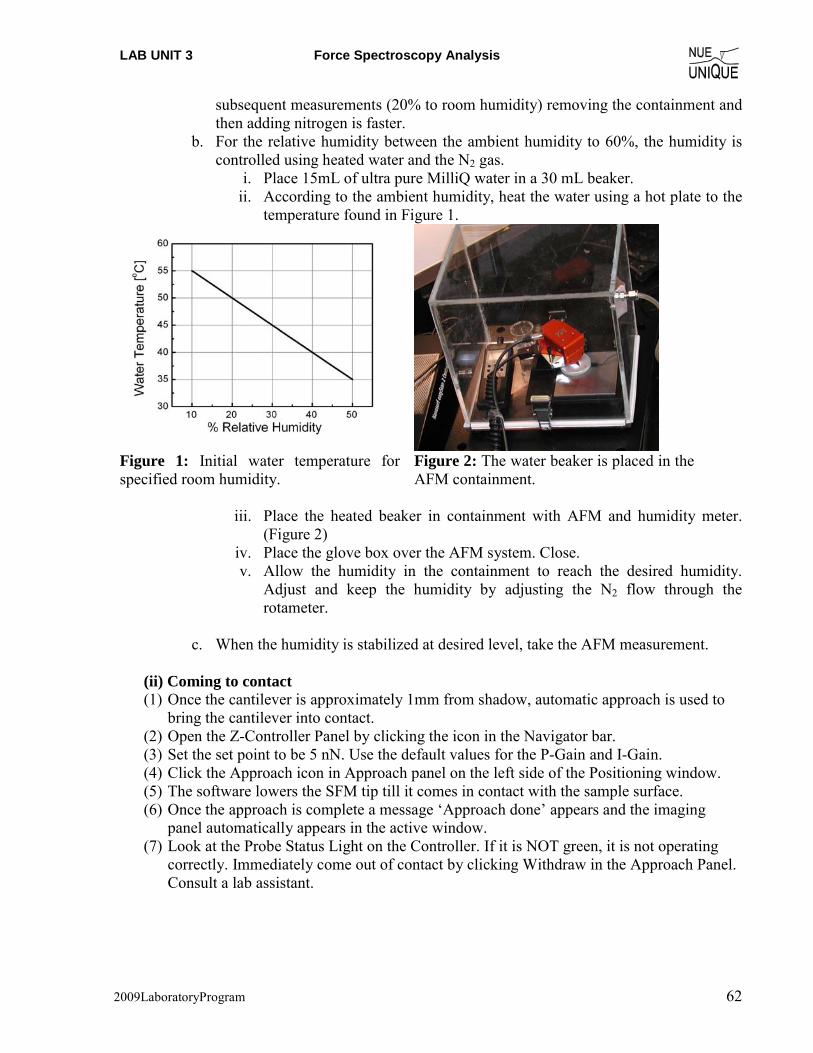
b. For the relative humidity between the ambient humidity to 60%, the humidity is controlled using heated water and the N2 gas.

i. Place 15mL of ultra pure MilliQ water in a 30 mL beaker. ii. According to the ambient humidity, heat the water using a hot plate to the

temperature found in Figure 1.

Figure 1: Initial water temperature for specified room humidity.

Figure 2: The water beaker is placed in the AFM containment.

iii. Place the heated beaker in containment with AFM and humidity meter.

(Figure 2) iv. Place the glove box over the AFM system. Close. v. Allow the humidity in the containment to reach the desired humidity.

Adjust and keep the humidity by adjusting the N2 flow through the rotameter.

c. When the humidity is stabilized at desired level, take the AFM measurement.

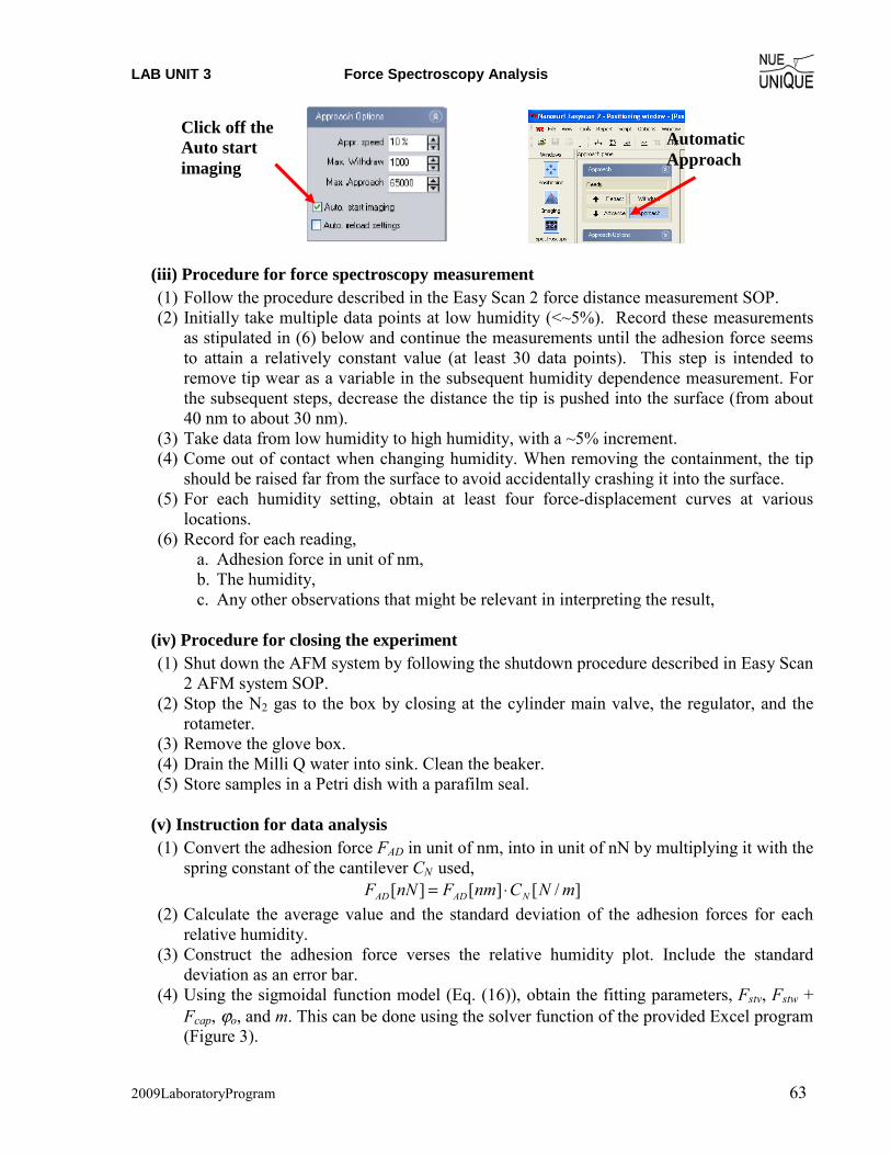
(ii) Coming to contact (1) Once the cantilever is approximately 1mm from shadow, automatic approach is used to

bring the cantilever into contact. (2) Open the Z-Controller Panel by clicking the icon in the Navigator bar. (3) Set the set point to be 5 nN. Use the default values for the P-Gain and I-Gain. (4) Click the Approach icon in Approach panel on the left side of the Positioning window. (5) The software lowers the SFM tip till it comes in contact with the sample surface. (6) Once the approach is complete a message ‘Approach done’ appears and the imaging

panel automatically appears in the active window. (7) Look at the Probe Status Light on the Controller. If it is NOT green, it is not operating

correctly. Immediately come out of contact by clicking Withdraw in the Approach Panel. Consult a lab assistant.



(iii) Procedure for force spectroscopy measurement

(1) Follow the procedure described in the Easy Scan 2 force distance measurement SOP. (2) Initially take multiple data points at low humidity (<~5%). Record these measurements

as stipulated in (6) below and continue the measurements until the adhesion force seems to attain a relatively constant value (at least 30 data points). This step is intended to remove tip wear as a variable in the subsequent humidity dependence measurement. For the subsequent steps, decrease the distance the tip is pushed into the surface (from about 40 nm to about 30 nm).

(3) Take data from low humidity to high humidity, with a ~5% increment. (4) Come out of contact when changing humidity. When removing the containment, the tip

should be raised far from the surface to avoid accidentally crashing it into the surface. (5) For each humidity setting, obtain at least four force-displacement curves at various

locations. (6) Record for each reading,

a. Adhesion force in unit of nm, b. The humidity, c. Any other observations that might be relevant in interpreting the result,

(iv) Procedure for closing the experiment

(1) Shut down the AFM system by following the shutdown procedure described in Easy Scan 2 AFM system SOP.

(2) Stop the N2 gas to the box by closing at the cylinder main valve, the regulator, and the rotameter.

(3) Remove the glove box. (4) Drain the Milli Q water into sink. Clean the beaker. (5) Store samples in a Petri dish with a parafilm seal.

(v) Instruction for data analysis

(1) Convert the adhesion force FAD in unit of nm, into in unit of nN by multiplying it with the spring constant of the cantilever CN used,

]/[][][ mNCnmFnNF NADAD ⋅= (2) Calculate the average value and the standard deviation of the adhesion forces for each

relative humidity. (3) Construct the adhesion force verses the relative humidity plot. Include the standard

deviation as an error bar. (4) Using the sigmoidal function model (Eq. (16)), obtain the fitting parameters, Fstv, Fstw +

Fcap, ϕo, and m. This can be done using the solver function of the provided Excel program (Figure 3).

Automatic Approach

Click off the Auto start imaging



a. Input the relative humidity (x-axis) and the average adhesion force (y-axis) into the cells (light green) of the Excel work sheet. The program will generate the plot.

b. Set the Fcap+Fstw cell to the maximum observed adhesion force and the Fstv to the minimum observed adhesion force as initial guesses. Initial guesses for ϕo, and m should be 100 and 5, respectively.

c. Open Tool on the tool bar and select Solver d. Set the Target Cell by selecting the yellow cell indicated in the work sheet. e. Select Equal to “Min” (minimize) f. Select By Changing Cells the parameter cells indicated by purple in the worksheet. g. Click on Solve to obtain the best values for the fit parameters. h. The fit parameters will appear automatically in the purple cells. i. If the fit curve does not substantially resemble the data different initial guess values

may be required. Consult your teaching assistant.

Figure 3: Data analysis within Excel (use of Solver Function)

(5) Using the value of Fstv obtained experimentally, the tip radius R can be deduced using Eq. (17a). The Wstv can be obtained through Eq. (18).

(6) Using the value R, calculate Fstw (Eq. (17b)). (7) Fcap is calculated by subtracting Fstw from experimentally determined value of (Fstw +

Fcap) (from step (4)). (8) Using the capillary equation with geometric coefficient K (Eq. (19)), calculate the filling

angle φ.

Additional information: Contact Angle (silicon/water) = 0°

By Changing Cells

Equal To

Set Target Cell



γSiO/air = 100 mJ/m2 γSiO/waterr = 24.5 mJ/m2 γwater = 72.8 mJ/m2

(v) Silicon Treatment Prior to Experiment

The pretreatment of silicon addresses organic condamination. Safety (1) Follow the general rules for Nanotechnology Wet-Chemistry Lab at your Institution. (2) The UV/Ozone cleaner should be OFF before opening the sample tray. (3) Always handle silicon wafers with tweezers, not with your fingers. Wafer edges can be very sharp. (4) All solvent wastes are disposed into designated waste bottles located under the hood. (5) All silicon waste are disposed into the sharp object waste box. Depending on the degree of condamination solvent cleaning and UV/Ozone treatment are recommended.

Materials (1) 4 pieces of Silicon wafers ( ~1cm2 size pieces) (2) Millipore H2O (3) Acetone (4) Methanol (5) A 150 ml beaker, a caddy and a watch glass for sonication (6) A waste beaker for organic solvent (7) A plastic waste beaker. (8) Fine point tweezers (9) N2 gas with 0.2 micron filter. (10) 3 Petri dishes and para-film for finished samples. (11) UV/Ozone cleaner. (12) Sonicator (13) DI water

Procedure (1) Solvent cleaning: Removes organics off of the silicon surfaces.

a. Place silicon wafers in the caddy fitted in a 150 ml beaker and pour Acetone to fill upto~ 60 ml. b. Fill the sonicator with water. Place the beaker and adjust amount of water so that the water in the

sonicator is about at the surface level of Acetone in the beaker. c. Cover with the watch glass. d. Turn on the sonicator and run for 15 minutes. e. Turn off the sonicator and remove the beaker. f. Lift up the caddy (with silicon wafers) and drain the acetone into a waste beaker. Place the caddy

back into the beaker. g. Pour small amount of methanol for rinsing. Drain the methanol into the waste beaker. Repeat

once. h. Fill the beaker with Methanol upto ~ 60 ml. i. Place the beaker back in to the sonicator. Cover with the watch glass. j. Sonicate for 30 minutes. Take the beaker out when done. k. Lift the caddy and pour out the methanol into the waste beaker. Rinse with Millipore water at least

three times. Return the caddy back into the beaker and fill with Millipore water. l. Pick up a piece of wafers with tweezers and rinse with flowing Millipore water. Blowdry it with

N2 gas. m. Place the dried silicon wafers in a Petri dish. Cover the Petri dish.



n. Transfer the waste solvent mixture (of acetone, methanol and water) into the designated solvent waste bottle. Rinse the waste beaker with DI water. The spent water is also drained into the waste bottle. Note: Don’t use this waste beaker for the HF process.

o. Empty out the sonicator and allow drying.

(2) UV/Ozone treatment: Removes any trace of organics off of the surface.

a. Make sure the UV/Ozone cleaner is OFF. b. Open the sample tray and place two of the silicon wafers. Leave the other two for HF treatment. c. Close the tray. d. Turn on the power switch. e. Set a timer to 30 minutes and start. f. Turn of the power switch when done. Open the sample tray and take the silicon wafers out and

place them into a Petri dish and seal it with parafilm.



4. Background: Non-Covalent Short Range Interactions and Capillary Forces Table of Contents:

Motivation ................................................................................................................. 67 Short Range Interactions and Surface Forces............................................................ 67 Van der Waals Interactions for Point Interactions .................................................... 69 Surface Forces ........................................................................................................... 70 Hamaker Constant ..................................................................................................... 71 Van der Waals Retardation Effects ........................................................................... 72 Adhesion and Surface Energies................................................................................. 72 Cutoff Distance for Van der Waals Calculations ...................................................... 73 Capillary Forces due to Vapor Condensation ........................................................... 74 Critical Humidity for Capillary Neck Formation ...................................................... 75 Estimation of the Tip Radius Utilizing the Capillary Effects ................................... 76 Modification of Hydrophobicity (Wettability).......................................................... 78 Force Displacement Curves ...................................................................................... 79 References ................................................................................................................. 80 Recommended Reading............................................................................................. 80

Motivation As technology moves more towards miniaturization in novel product developments, it is

imperative to integrate interfacial interactions into design strategies. Consequently, interfacial forces have to be explored. Interfacial forces are on the order of 10-6 to 10-10 N, strong enough, for instance, to freeze gears in micro-electrical mechanical systems (MEMS), to affect the stability of colloidal system, or to wipe out magnetically stored data information in hard drives. There are multiple ways of exploring the strength of interfacial interactions, one of which is by force spectroscopy, also known as force-displacement (FD) analysis. The FD analysis involves a nanometer sharp scanning force microscopy (SFM) tip that is moved relative to the sample surface in nanometer to micrometer per second, as illustrated at end of this document in Figure 10. Before we discuss FD analysis, we first discuss interaction forces, particularly weak interactions between molecules and solids.

Short Range Interactions and Surface Forces There are three aspects that are of particular importance for any interaction: Its strength,

the distance over which it acts, and the environment through which it acts. Short range interactions, as summarized in Table 1, can be of following nature: ionic, covalent, metallic, or dipolar origin. Ionic, covalent, metallic and hydrogen bonds are so-called atomic forces that are important for forming strongly bonded condensed matter. These short range forces arise from the overlap of electron wave functions. Interactions of dipolar nature are classified further into strong hydrogen bonds and weak Van der Waals (VdW) interactions. They arise from dipole-



dipole interactions. Both hydrogen and VdW interactions can be responsible for cooperation and structuring in fluidic systems, but are also strong enough to build up condensed phases. Following is a description of these short range forces:

A. Ionic Bonds: These are simple Coulombic forces, which are a result of electron transfer.

For example in lithium fluoride, lithium transfers its 2s electron to the fluorine 2p state. Consequently the shells of the atoms are filled up, but the lithium has a net positive charge and the Flourine has a net negative charge. These ions attract each other by Coulombic interaction which stabilizes the ionic crystal in the rock-salt structure.

B. Covalent Bond: The standard example for a covalent bond is the hydrogen molecule. When the wave-function overlap is considerable, the electrons of the hydrogen atoms will be indistinguishable. The total energy will be decreased by the “exchange energy”, which causes the attractive force. The characteristic property of covalent bonds is a concentration of the electron charge density between two nuclei. The force is strongly directed and falls off within a few Ǻngstroms.

C. Metallic Bonds and Interaction: The strong metallic bonds are only observed when the atoms are condensed in a crystal. They originate from the free valence electron sea which holds together the ionic core. A similar effect is observed when two metallic surfaces approach each other. The electron clouds have the tendency to spread out in order to minimize the surface energy. Thus a strong exponentially decreasing, attractive interaction is observed.

D. Dipole Interactions:

D.1. Hydrogen Bond Interaction: Strong type of directional dipole-dipole interaction

D.2. Van der Waals Interaction: The relevance of VdW interactions goes beyond of building up matter (e.g., Van der Waals organic crystals (Naphthalene)). Because of their “medium” range interaction length of a few Ǻngstroms to hundreds of Ǻngstroms, VdW forces are significant in fluidic systems (e.g, colloidal fluids), and for adhesion between microscopic bodies. VdW forces can be divided into three groups: o Dipole-dipole force: Molecules having permanent dipoles will interact by dipole-

dipole interaction. o Dipole-induced dipole forces: The field of a permanent dipole induces a dipole in

a non-polar atom or molecule. o Dispersion force: Due to charge fluctuations of the atoms there is an

instantaneous displacement of the center of positive charge against the center of the negative charge. Thus, at a certain moment, a dipole exists and induces a dipole in another atom. Therefore non-polar atoms (e.g. neon) or molecules attract each other.

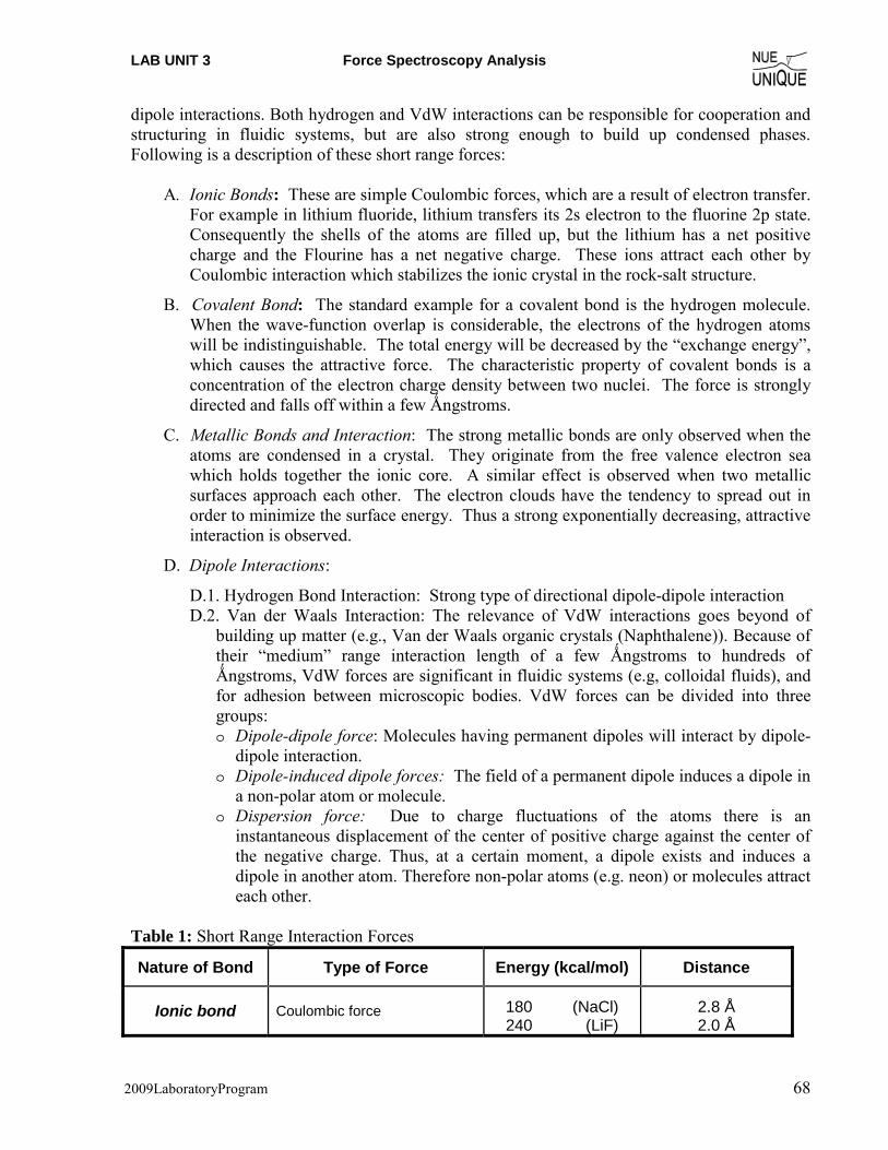
Table 1: Short Range Interaction Forces

Nature of Bond Type of Force Energy (kcal/mol) Distance

Ionic bond Coulombic force

180 (NaCl) 240 (LiF)

2.8 Å 2.0 Å



Covalent bond Electrostatic force (wave function overlap)

170 (Diamond) 283 (SiC)

N/A

Metallic bond free valency electron sea interaction (sometimes also partially covalent (e.g., Fe and W)

26 (Na) 96 (Fe) 210 (W)

4.3 Å 2.9 Å 3.1 Å

Hydrogen Bond a strong type of directional dipole-dipole interaction

7 (HF)

Van der Waals (i) dipole-dipole force (ii) dipole-induced dipole force (iii) dispersion forces (charge fluctuation)

2.4 (CH4)

significant in the range of a few Å to hundreds of Å

Van der Waals Interactions for Point Interactions The attractive VdW pair potential between point particles (i.e., atoms or small nonpolar

spherical molecule) is proportional to 1/r6, where r is the distance between the point particles. The widely used semi-empirical potential to describe VdW interactions is the Lennard-Jones (LJ) potential, referred to as the 6-12 potential because of its (1/r)6 and (1/r)12 distance r dependence of the attractive interaction and repulsive component, respectively. While the 6-potential is derived from point particle dipole-dipole interaction, the 12-potential is based on pure empiricism. The LJ potential is provided in the following two equivalent forms as function of the particle-particle distance r:

⎥⎥

⎦

⎤

⎢⎢

⎣

⎡⎟⎠

⎞⎜⎝

⎛ σ−⎟⎠

⎞⎜⎝

⎛ σε=+−=φ612

126 4rrr

C

rC)r( repvdw (1a)

where

rep

vdw

vdw

rep

CC;

CC

4

261

=ε⎟⎟⎠

⎞⎜⎜⎝

⎛=σ (1b)

Cvdw and Crep are characteristic constants. C = Cvdw is called the VdW interaction parameter. The empirical constant ε represents the characteristic energy of interaction between the molecules (the maximum energy of attraction between a pair of molecules). σ, a characteristic diameter of the molecule (also called the collision diameter), is the distance between two atoms (or molecules) for φ(r) = 0. The LJ potential is depicted in Figure 4..

Surface Forces The integral form of interaction forces between surfaces of macroscopic bodies through a third medium (e.g., vacuum and vapor) are called surfaces forces. To apply the VdW formalism to macroscopic bodies, one has to integrate the point interaction form presented above.

Figure 4: Lennard Jones (6-12) potential (empirical Van der Waals Potential between two atoms or nonpolar molecules).

r

φ(ε)

0

r(ε)

ε

σ

-



Consequently, the dipole-dipole interaction strength C but also the exponent of the distance dependence become geometry dependent. For instance, while for point-point particles the exponent is -6, it is -1 and -3 for macroscopic sphere-sphere and sphere-plane interactions, respectively. Thus, while, VdW point particle interactions are very short ranged (~1/r6), macroscopic VdW interactions are long ranged (e.g., sphere-sphere: ~1/D, where D represents the shortest distance between the two macroscopic objects). Table 3 provides a list of geometry dependent non-retarded VdW interaction strengths and exponents.

In vacuum, the main contributors to long-range surface interactions are the Van der Waals and electromagnetic interactions. At separation distance < 2 nm one might also have to consider short range retardation due to covalent or metallic bonding forces. Van der Waals and electromagnetic interactions can be both attractive or repulsive. In the case of a vapor environment as the third medium (e.g., atmospheric air containing water and organic molecules), one also has to consider modifications by the vapor due to surface adsorption or interaction shielding. This can lead to force modification or additional forces such as the strong attractive capillary forces.

The SFM tip-sample interaction potential W are typically modeled as a sphere-plane interaction, i.e.,

DAR)D(W

6−= (2a)

with the force 26D

AR)D(FDW −==−�

� (2b)

where R is the radius of curvature of the tip, and D is the distance between the tip and the plane. The interaction constant A, is called the Hamaker constant, defined as A = π2Cρ1ρ2, with the interaction parameter of the point-point interaction C, and the number density of the molecules in both solids ρi (i = 1,2). The Hamaker constant is based on the mean-field Lifshitz theory. If known, A provides the means to deduce the material specific (i.e., geometry independent) interaction parameter C. Typical values for A, C and ρ are provided in Table 2. Table 3 summarizes the Van der Waals interaction potential for various geometries.

Table 2: Hamaker constants of Hydrocarbon, CCl4, and water.

Medium C (10-79 Jm6) ρ [1028m-3] A [10-19 J] Hydrocarbon 50 3.3 0.5

CCl4 1500 0.6 0.5 Water 140 3.3 1.5

Table 3: Van der Waals interaction Potential



Interaction Potential (W)

Two Atoms

Atom-Surface

Sphere-Sphere

Plane-Sphere

Two Cylinders

Two Crossed Cylinders

Plane-Plane

Two Parallel Chain Molecules

Poin

t Int

erac

tion

Bod

y In

tera

ctio

n

Geometry of Interaction

6rC−

36DCρπ−

)(6 21

21

RRRR

DA

+−

DAR

6−

21

21

2123 )(212 ⎟⎟

⎠

⎞⎜⎜⎝

⎛

+ RRRR

DAL

DRRA

621−

212 DA

π−

5283

rCL

σπ−

Hamaker Constant Originally the Hamaker constant was determined based on a purely additive method in

which polarization was ignored. The Lifshitz theory has overcome the problem of additivity. It is a continuum theory which neglects the atomic structure. The input parameters are the dielectric constants, ε, and refractive indices, n. The Hamaker constant for two macroscopic phases 1 and 2 interacting across a medium 3 is approximated as:

( )( )( ) ( ) ( ) ( ){ }2

32

22

32

12

32

22

32

1

23

22

23

21

32

32

31

31

283

43

nnnnnnnn

nnnnhkTA e

+++++

−−+⎟⎟⎠

⎞⎜⎜⎝

⎛

+−

⎟⎟⎠

⎞⎜⎜⎝

⎛

+−≈ υ

εεεε

εεεε (3)

where νe is the absorption frequency (e.g., for H2O: νe = 3 x 1015 Hz). Table 4 provides non-retarded Hamaker constants determined with the Lifshitz theory (eq. 3). In general, there is an attractive VDW interaction for A > 0, and the two macroscopic phases are attracted to each other. In cases where it is desired to have repulsive forces, the medium must have dielectric properties which are intermediate to the macroscopic phases.

Table 4: Non-retarded Hamaker constants for two interacting media across a vacuum (air) (Source: intermolecular & Surface Forces, J. Israelachvili, Academic Press) 3



Dielectric constant Refractive Index Absorption frequencya Hamaker Constant

ε n ν Amedium/air/medium

Medium (1015s-1) (10-20)

Acetone 21 1.359 2.9 4.1

Benzene 2.28 1.501 2.1 5.0

Calcium Flouride 7.4 1.427 3.8 7.0

Carbon tetrachloride 2.24 1.460 2.7 5.5

Cyclohexane 2.03 1.426 2.9 5.2

Ethanol 26 1.361 3.0 4.2

Fused quartz 3.8 1.448 3.2 6.3

Hydrocarbon (crystal) 2.25 1.50 3.0 7.1

Iron oxide (Fe3O4) 1.97 3.0 est 21

Liquid He 1.057 1.028 5.9 0.057

Metals (Au. Ag, Cu) 3-5 25--40

Mica 7.0 1.60 3.0 10

n-Pentane 1.84 1.349 3.0 3.8

n-Octane 1.95 1.387 3.0 4.5

n-Dodecane 2.01 1.411 3.0 5.0

n-Tetradecane 2.03 1.418 2.9 5.0

n-Hexadecane 2.05 1.423 2.9 5.1

Polystyrene 2.55 1.557 2.3 6.5

Polyvinyl chloride 3.2 1.527 2.9 7.5

PTFE 2.1 1.359 2.9 3.8

Water 80 1.333 3.0 3.7aUV absorption frequencies obtained from Cauchy plots mainly from Hough and White (1980) and H. Christenson (1983, thesis).

Van der Waals Retardation Effects The van der Waals forces are effective from a distance of a few Ǻngstroms to several hundreds of Ǻngstroms. When two atoms are a large distance apart, the time for the electric field to return can be critical, i.e., comparable to the fluctuating period of the dipole itself. The dispersion can be considered to be retarded for distances more than 100 Å, i.e., the dispersion energy begins to decay faster than 1/r6 (~1/r7). It is important to note that for macroscopic bodies retardation effects are more important than for atom-atom interactions. This is of particular importance for the SFM force displacement method.

Adhesion and Surface Energies The energy of adhesion (or just adhesion), W", i.e., the energy per unit area necessary to

separate two bodies (1 and 2) in contact, defines the interfacial energy γ12 as: 21211212 22 γγγγγγ −+== ;W '' (4)

where γi (i= 1,2) represent the two surface energies. Assuming two planar surfaces in contact, the Van der Waals interaction energy per unit area is

( ) 21 12 DADW

π−= (see above) (5)

which was obtained by pairwise summation of energies between all the atoms of medium 1 with medium 2. The summation of atom interactions within the same medium have been neglected, which yields additional energy terms, i.e.,

22 12 oDA.constW

π+−= (6)



consisting of a bulk cohesive energy term (assumed to be constant), and an energy term related to unsaturated "bonds" at the two surfaces in contact (i.e., D = Do). Notice that contact cannot be defined as D = 0 due to molecular repulsive forces. Do is called the "cutoff distance". Hence the total energy of two planar surfaces at a distance D ≥ Do apart is (neglecting the bulk cohesive energy)

⎟⎟⎠

⎞⎜⎜⎝

⎛−=⎟⎟

⎠

⎞⎜⎜⎝

⎛−−=+= 2

2

22221 112

1112 D

DDA

DDAWWW o

oo ππ. (7)

In contact (i.e., D=Do) W = 0. In the case of isolated surfaces, i.e., D = ∞, 212 oD

AWπ

= . (8)

Thus, in order to separate the two surfaces one has to overcome the energy difference

ΔW=W(Do)- W(D=∞)=- 212 oDA

π, (9)

which corresponds to the adhesive energy per unit area of W''=2γ12. Hence, the interfacial energy can expressed as function of the Hamaker constant and the cutoff distance:

212 24 oDAπ

γ = , (10)

Cutoff Distance for Van der Waals Calculations The challenge is to determine the repulsive cutoff distance Do, which unfortunately

cannot be set equal to the collision diameter, σ (i.e., the distance between atomic centers). Let us assume a planar solid consisting of atoms that are close-packed. Each surface atom (of diameter σ) will have nine nearest neighbors (instead of 12 as in the bulk). When surface atoms come into contact with a second surface each atom will gain (12-9)w=3w=3C/σ6 in binding energy. Thus, the energy per unit area, S=σ2sin(60 deg) = σ2√3/2, is

32

2

8122

2333

21

σρ

σρ

σγ ===⎟

⎠

⎞⎜⎝

⎛= ;CCSw , (11)

where ρ reflects the bulk atom density for a close packed system. Introducing the definition of the Hamaker constant, it follows

2222

2

12

5224

23

23

⎟⎠

⎞⎜⎝

⎛≈==

.

AACσπ

σπσργ , (12)

For σ = 0.4 nm and γ12 = A/(24πDo2) it follows that Do = 0.16 nm. Do = 0.16 nm is a remarkable

"universal constant" yielding values for surface energies γ that are in good agreement with experiments as shown in the Table 5.

Table 5: Surface energies based on Lifshitz theory and experimental values.(Source: intermolecular & Surface Forces, J. Israelachvili, Academic Press) 3



Lifshiz Theory

A/24 π Do2

(10 -20) {Do=0.165nm} (20oC)

Liquid helium 0.057 0.28 0.12 - 0.35(at 4-1.6K)

Water 3.7 18 73

Acetone 4.1 20.0 23.7Benzene 5.0 24.4 28.8CCl4 5.5 26.8 29.7H2o2 5.4 26 76Formamide 6.1 30 58

Methanol 3.6 18 23Ethanol 4.2 20.5 22.8Glycerol 6.7 33 63Glycol 5.6 28 48

n- Pentane 3.75 18.3 16.1n -Hexadecane 5.2 25.3 27.5n -Octane 4.5 21.9 21.6n -Dodecane 5.0 24.4 25.4Cyclohexane 5.2 25.3 25.5

PTFE 3.8 18.5 18.3Polystyrene 6.6 32.1 33Polyvinyl chloride 7.8 38.0 39

Material A

Surface Energy, γ (mJ/m2)

Experimental*

Capillary Forces due to Vapor Condensation In the discussion above we have considered a continuous medium in-between the two

surfaces to deduce the surface forces. Thereby, we have assumed that this third medium fills up the vacuum space entirely, i.e., does not introduce interfaces. We have to drop this assumption, however, should the third medium form a finite condensed phase within the interaction zone of the two bodies. Any condensed phase within the interaction zone will exhibit interfaces towards the vapor, and thus, if deformed (e.g., stretched) contribute to the acting forces. These new forces, called capillary forces, are on the order of 10-7 N for single asperity contacts with radii of curvatures below 100 nm.

Capillary forces are meniscus forces due to condensation. It is well known that micro-contacts act as nuclei of condensation. In air, water vapor plays the dominant role. If the radius of curvature of the micro-contact is below a certain critical radius, a meniscus will be formed. This critical radius is defined approximately by the size of the Kelvin radius rK = l/(l/rl + 1/r2) where rl and r2 are the radii of curvature of the meniscus. The Kelvin radius is connected with the partial pressure ps (saturation vapor pressure) by

⎟⎟⎠

⎞⎜⎜⎝

⎛=

s

LK

pplogRT

Vr γ , (13)



where γL is the surface tension, R the gas constant, T the temperature, V the mol volume and p/ps

the relative vapor pressure (relative humidity for water). The surface tension γL of water is 0.074N/m (T=20°C) leading to a critical Van der Waals distance of water of γLV/RT = 5.4 Å. Consequentially, we obtain for p/ps=0.9 a Kelvin radius of 100 Å. At small vapor pressures, the Kelvin radius gets comparable to the dimensions of the molecules, and thus, the Kelvin equation breaks down. The meniscus forces between two objects of spherical and planar geometry can be approximated, for D « R, as:

( )d/DcosRF LDR

+Θ=>>

14 γπ , (14)

where R is the radius of the sphere, d the length of PQ , see Figure 5, D the distance between the sphere and the plate, and θ the meniscus contact angle.

Figure 5: Capillary meniscus between two objects of spherical and planar geometry

The maximum force, found at at D = 0 (contact), is θγπ cosRF dR

max 4=>> . While this expression estimates the capillary forces of relatively large spheres fairly accurately, the capillary forces of highly wetted nanoscale spheres requires a geometrical factor K.

φφ

cos4)cos1( 2

⋅+=K (15)

where φ is the filling angle.

Critical Humidity for Capillary Neck Formation SFM force displacement analysis studies involving hydrophilic counter-surfaces and

water vapor have identified three humidity regimes with significantly different involvement of the third medium, as shown in Figure 6. At very low humidity (regime I), below a critical relative humidity (RH) of ~40 %, no capillary neck is developed, and the forces measured truly reflects VdW interactions. A capillary neck is formed at about 40 % RH, which leads to a force discontinuity observed between regimes I and II. We can understand this transition-like behavior of the pull-off force by considering the minimum thickness requirement of a liquid precursor film for spreading. The height of the precursor film can not drop below a certain minimum, e, which is



2/1

0 ⎟⎠

⎞⎜⎝

⎛=S

ae γ ; 2/1

0 6 ⎟⎟⎠

⎞⎜⎜⎝

⎛=πγAa ; γγγ −−= SLSOS , (15)

where ao is a molecular length, S the spreading coefficient, A the Hamaker constant, γSO the solid-vacuum interfacial energy, and γSL the solid-liquid interfacial energy. As the water vapor film thickness depends on the RH (i.e., p/ps), a relative humidity smaller than 40 % does not provide a minimum thickness for the formation of a capillary neck. Once a capillary neck forms between the SFM tip and the substrate surfaces, the pull-off force increases suddenly, and provides over regime II a pull-off force that contains both, VdW and capillary forces. VdW forces from SFM FD analysis as determined, for instance, from regime I, see Figure 6(b), are on the order of 1-10 nN. The capillary force, on the other hand, is on the order of up to 100 nN, and thus, dominates VdW interactions in regime II.

Pull-

off F

orce

Relative Humidity

I II III

Figure 6(a): Generic sketch of the functional relationship between the pull-off force and the relative humidity (RH). Regimes I, II and III represent the van der Waals regime, mixed van der Waals – capillary regime, and capillary regime decreased by repulsive forces, respectively.

Figure 6(b): Pull-off force vs. RH measured between a hydrophilic silicon oxide SFM tip and a ultra-smooth silicon oxide wafer. ● measured for increasing RH, ▼ measured for decreasing RH. .1

In the high RH regime (III) the pull-off force decreases with increasing RH for

hydrophilic counter-surfaces. At such high humidity, the water vapor film thickness dimensions exceeds the contact size (� asperity flooding), and the effect of the capillary interface decreases.

Estimation of the Tip Radius Utilizing the Capillary Effects The capillary effect, commonly not desired, can be useful in estimating the SFM tip

radius. Assuming the absence of the flooding effect and the ionic salvation effect within regime III, as discussed in the previous section, the humidity dependent adhesion forces can be described as a mathematical model of sigmoidal form4,

]m/)exp[()FF(F

)FF(F capstwstvcapstwmea

01 ϕϕ −+

+−++= (16)

where Fmea is the experimentally determined pull-off forces,

Fstv is the van der Waals interaction force between the sample and the tip in water vapor,



Fstw is the van der Waals interaction force between the sample and the tip in liquid water,

Fcap is the capillary force, φ is the relative humidity (in fraction), ϕ0 is the mid-point of the transition regime, and m is the transition width.

As shown in Figure 7, the forces, Fstv, Fstw, and Fcap, are components of the measured pull-off force Fmea. When the relative humidity is below the transition regime, i.e., ϕ < ϕ0, the Fmea consists Fstv only, represents the lower limit of the sigmoidal fit. Above the transition regime, Fmea is the sum of Fstw and Fcap, represents the upper limit of the sigmoidal fit.

Figure 7: The components of full-off forces in humid environment.

The Fstw and Fstv can be expressed by assuming that the contact is between an incompressible sphere and a hard flat surface, i.e. Bradley’s model (see page 24),

stvstv WRF ⋅⋅= π2 or stwstw WRF ⋅⋅= π2 (17a or 17b) where R is the sphere radius (i.e. SFM tip radius), W is the work of adhesion which is expressed as,

ijjmimijmW γγγ ++= (18) where γ is the interfacial energies of the two materials, and i, j, m represents solid i, solid j, and the medium m in which the contact take place, respectively. If the contact is between two solids with the same material, i.e., i = j, Eq. (18) reduces to imijmW γ2= . In order to determine the tip radius R, Eq. (17a) is solved for R using experimentally determined Fstv. The R value is then used to determine Fstw through Eq. (17b), and Fcap is deduced. Employing the geometric coefficient K for the capillary force equation,

φφθγπ

cos4)cos1(cos4

2

⋅+⋅⋅⋅= watercap RF (19)

the filling angle φ can be deduced. For example, the result obtained by He et. al.1 on the silicon wafer surface, was analyzed using this model. Using the value of γ SiO/air 100 mJ/m2, γSiO/water 24.5 mJ/m2, γ water 72.8 mJ/m2, and the contact angle Θ of 0 °, the tip radius R and the filling angle φ was determined to be 8.7 nm and 85.6 ° respectively.5



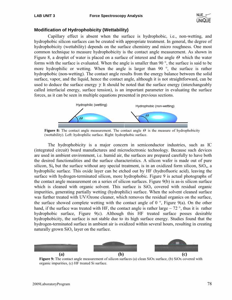
Modification of Hydrophobicity (Wettability) Capillary effect is absent when the surface is hydrophobic, i.e., non-wetting, and hydrophobic silicon surfaces can be created with appropriate treatment. In general, the degree of hydrophobicity (wettability) depends on the surface chemistry and micro roughness. One most common technique to measure hydrophobicity is the contact angle measurement. As shown in Figure 8, a droplet of water is placed on a surface of interest and the angle Θ which the water forms with the surface is evaluated. When the angle is smaller than 90 °, the surface is said to be more hydrophilic or wetting. When the angle is larger than 90 °, the surface is rather hydrophobic (non-wetting). The contact angle results from the energy balance between the solid surface, vapor, and the liquid, hence the contact angle, although it is not straightforward, can be used to deduce the surface energy γ. It should be noted that the surface energy (interchangeably called interfacial energy, surface tension), is an important parameter in evaluating the surface forces, as it can be seen in multiple equations presented in previous sections.

Figure 8: The contact angle measurement. The contact angle Θ is the measure of hydrophobicity (wettability). Left: hydrophilic surface. Right: hydrophobic surface.

The hydrophobicity is a major concern in semiconductor industries, such as IC (integrated circuit) board manufactures and microelectronic technology. Because such devices are used in ambient environment, i.e. humid air, the surfaces are prepared carefully to have both the desired functionalities and the surface characteristics. A silicon wafer is made out of pure silicon, Si, but the surface without any special treatment, is in an oxidized form silicon, SiOx, a hydrophilic surface. This oxide layer can be etched out by HF (hydrofluoric acid), leaving the surface with hydrogen-terminated silicon, more hydrophobic. Figure 9 is actual photographs of the contact angle measurement on a series of silicon surfaces. Figure 9(b) is as-is silicon surface which is cleaned with organic solvent. This surface is SiOx covered with residual organic impurities, generating partially wetting (hydrophilic) surface. When the solvent cleaned surface was further treated with UV/Ozone cleaner, which removes the residual organics on the surface, the surface showed complete wetting with the contact angle of 0 °, Figure 9(a). On the other hand, if the surface was treated with HF, the contact angle is rather large ~ 72 °, thus it is rather hydrophobic surface, Figure 9(c). Although this HF treated surface posses desirable hydrophobicity, the surface is not stable due to its high surface energy. Studies found that the hydrogen-terminated surface in ambient air is oxidized within several hours, resulting in creating naturally grown SiOx layer on the surface.

(a) (b) (c)

Figure 9: The contact angle measurement of silicon surfaces (a) clean SiOx surface, (b) SiOx covered with organic impurities, (c) HF treated Si surface.



Force Displacement Curves In SFM force displacement (FD) analysis, the normal forces acting on the cantilever are measured as a function of the tip-sample displacement. In other words, the tip-sample distance could not be precisely controlled due to the flexibility of the cantilever. As a result, the FD curve jumps the path of the force curve as illustrated in Figure 10. Figure 10(a) shows the cantilever approach from point Do. When the distance reaches point A0 an instability occurs resulting in a jump into contact to point B0. On the retraction out of contact an instability occurs at point C0 causing the cantilever tip to snap out of contact back to point D0. As a result the typical force distance curve is shown in Figure 10(b). Each segment of the curve is described as follows.

F(r)

CA

B

D

C0

D0

B0

A0

(a) (b) Figure 10: (a) The actual path taken by a SFM cantilever. The inset illustrates the snap-in instability at A0 where the second derivative of the interaction potential exceeds the spring constant of the cantilever. (b) Typical force distance curve. D = displacement, F(D) = force.

1. Line 1-A0: The probe and sample are not in contact but the tip is moving toward the

sample. 2. Line A0-B0: Jump into contact caused by the attractive van der Waals forces outweighing

the force of the cantilever spring between the tip and the sample causing the cantilever to bend.

3. Line B0-2: Shows upward deflection of the cantilever in response to the sample motion after they are in contact. The shape of the segment indicates whether the sample

is deforming in response to the force from the cantilever. (may not always be straight) If the sample is assumed to be a hard surface, the slope of this line is the sensitivity (springiness) of the cantilever.

4. Line 2-C0: As the tip moves away, the slope follows the slope of line B0-2 closely. If line 2-C0 is parallel to line B0-2, no additional information can be determined. However, if there is a difference in the in and out-going curves (hysteresis) gives information on the plastic deformation of the sample. Once it passes point 2’, the cantilever begins to deflect downward due to adhesive forces..

5. Line C0-D0: A jump out of contact occurs when the cantilever force exceeds the adhesive forces.



The jump out of contact distance will always be greater than the jump into contact distance because of few possible causes are:

a. During contact, some adhesive bonds are created. b. During contact, the sample buckles and “wraps” around the tip, increasing the

contact area. c. Hysteresis contributions d. Capillary forces exerted by contaminants such as water.

FD analysis is widely used for adhesion and force interaction studies. Recently biological

materials have been studied by force spectroscopy, such as adsorption strength of proteins on a substrate and folding/unfolding energy of DNAs.

References 1 M. He, A. Blum, D. E. Aston, C. Buenviaje, and R. M. Overney, Journal of chemical physics

114 (3), 1355 (2001). 2 H. Hertz, J. Reine und Angewandte Mathematik 92, 156 (1882). 3 J. N. Israelachvili, Intermolecular and surface forces. (Academic Press, London, 1992). 4 D. L. Sedin and K. L. Rowlen, Analytical Chemistry 72, 2183 (2000). 5 C. Ziebert and K. H. Zum Gahr, Tribology Letters 17 (4), 901 (2004). 6 J. A. Greenwood, Proc. R. Soc. Lond. A 453, 1277 (1997).

Recommended Reading

Contact Mechanics by K. L. Johnson, Cambridge University Press, Cambridge, 1985. Gases, liquids and solids and other states of matter by D. Tabor, Cambridge Univ. Press,

Cambridge, 3rd ed. 2000. Intermolecular and surface forces by J. N. Israelachvili, Academic Press, London, 1992. Nanoscience: Friction and Rheology on the Nanometer Scale by E. Meyer, R. M. Overney, K.

Dransfeld, and T. Gyalog, World Scientific Publ., Singapore, 1998.



5. Appendix The following MS-Excel based tools are provided. See Excel Toolbox.

Tool for Sigmoidal Data Fit

Lab Unit 1: Analysis Work Sheet

(2) Select "Solver" from Tools (3) Set the Target cell to the yellow cell(4) Select Min (minimum) for Equal to.(5) Set by Changing Cells to the purple cells(6) Click Solver to obtain the fit parameters (which appears to the purple cells)Note: DO NOT CHANGE the pink cells

m 0.80950955Fcap + Fstw 32.86757066

Fstv 10.58973278

ϕ0 40.39442756

Relative Humidity (%RH)

Average Fmea

[nN]Fit Model Sqrt

88.00 25.05 32.87 7.81293

81.70 29.40 32.87 3.46988

76.00 31.63 32.87 1.23269

70.40 33.33 32.87 0.46706

68.60 34.15 32.87 1.28173

62.39 35.05 32.87 2.18528

53.94 32.87 32.87 0.00002

42.51 31.34 31.34 0.00001

39.84 18.04 18.04 0.00001

33.00 11.57 10.59 0.97950

28.50 11.37 10.59 0.77533

22.90 11.04 10.59 0.45478

17.00 10.59 10.59 0.00000

12.40 10.43 10.59 0.16249

9.30 10.21 10.59 0.38416

8.50 10.01 10.59 0.57933Target Cell 19.78519

Fit Paramaters

(1) Input the values in the blue cells.

5

10

15

20

25

30

35

40

0.00 20.00 40.00 60.00 80.00

Relative Humidity [%RH]

Fmea

[nN

]

Fmea [nN]Fit Curve

]/)exp[(1)(

)(0

mFFF

FFF capstwstvcapstwmea ϕϕ −+

+−++=

Tool for Hamaker Constant Calculation (provided in Excel Toolbox)

Lab Unit 1: Hamaker Constant Calculation(1) Enter the given input parameters in the yellow boxes(2) Enter the given dielectric constants and refractive indices in the orange and green boxes respectively(3) The Hamaker constant and the interaction strength are given in the highlighted cells

T (K) 300k (J/K) 1.38E-23h (Js) 6.63E-34υε

(Hz) 3.00E+15R (nm) 50D0 (nm) 0.16

A[J] W[J]Phase 1 ε1 3.78 n1 1.45 5.97E-20 -3.11E-18Phase 2 ε2 3.78 n2 1.45Medium ε3 1 n3 1

Parameters

Dielectric Constants Refractive IndicesMaterial Properites

( )( )( ) ( ) ( ) ( ){ }2

32

22

32

12

32

22

32

1

23

22

23

21

32

32

31

31

283

43

nnnnnnnn

nnnnhkTA e

+++++

−−+⎟⎟⎠

⎞⎜⎜⎝

⎛

+−

⎟⎟⎠

⎞⎜⎜⎝

⎛

+−≈ υ

εεεε

εεεε

( )DARDW

6−=

lab unit 3: force spectroscopy...

Documents