Purdue University: ECE438 - Digital Signal Processing with Applications 1

ECE438 - Laboratory 4:

Sampling and Reconstructionof Continuous-Time Signals

October 6, 2010

1 Introduction

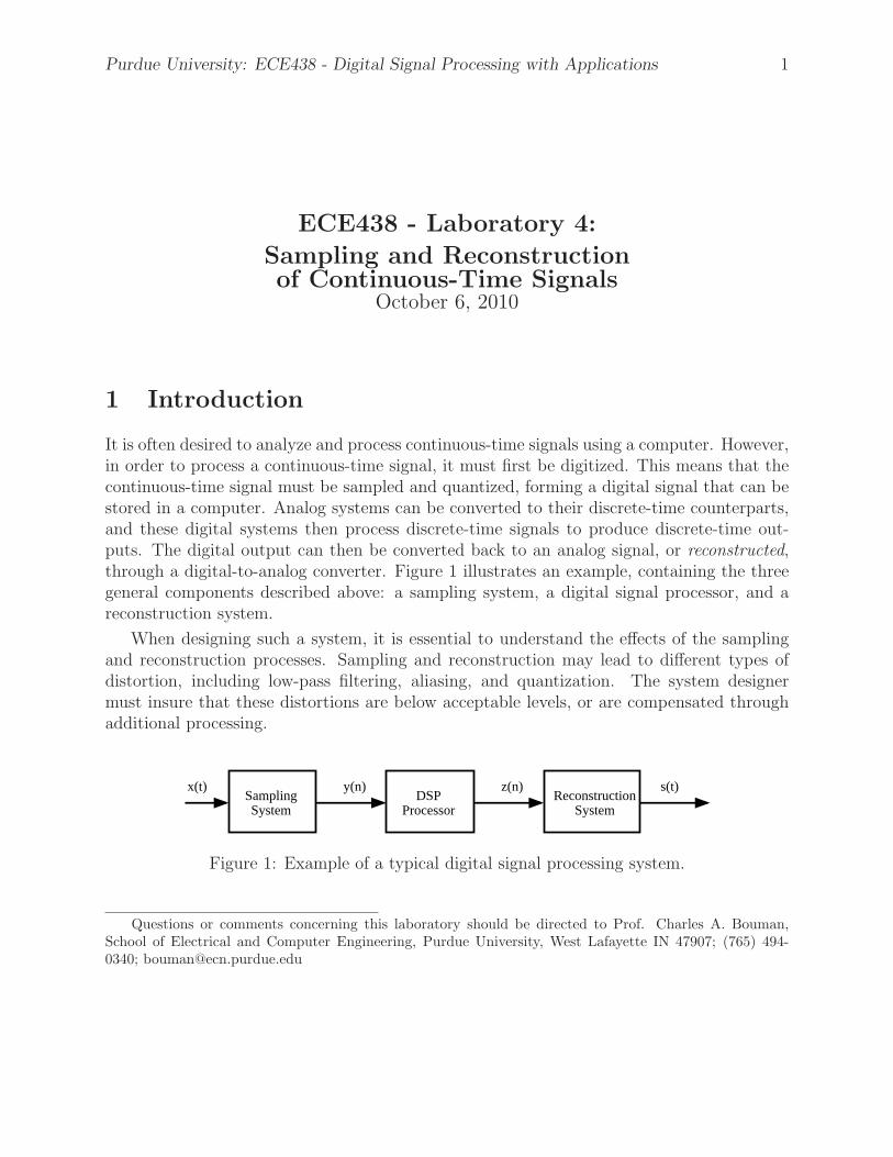
It is often desired to analyze and process continuous-time signals using a computer. However,in order to process a continuous-time signal, it must first be digitized. This means that thecontinuous-time signal must be sampled and quantized, forming a digital signal that can bestored in a computer. Analog systems can be converted to their discrete-time counterparts,and these digital systems then process discrete-time signals to produce discrete-time out-puts. The digital output can then be converted back to an analog signal, or reconstructed,through a digital-to-analog converter. Figure 1 illustrates an example, containing the threegeneral components described above: a sampling system, a digital signal processor, and areconstruction system.

When designing such a system, it is essential to understand the effects of the samplingand reconstruction processes. Sampling and reconstruction may lead to different types ofdistortion, including low-pass filtering, aliasing, and quantization. The system designermust insure that these distortions are below acceptable levels, or are compensated throughadditional processing.

SamplingSystem

DSPProcessor

ReconstructionSystem

x(t) y(n) z(n) s(t)

Figure 1: Example of a typical digital signal processing system.

Questions or comments concerning this laboratory should be directed to Prof. Charles A. Bouman,School of Electrical and Computer Engineering, Purdue University, West Lafayette IN 47907; (765) 494-0340; bouman@ecn.purdue.edu

Purdue University: ECE438 - Digital Signal Processing with Applications 2

1.1 Sampling Overview

Sampling is simply the process of measuring the value of a continuous-time signal at certaininstants of time. Typically, these measurements are uniformly separated by the samplingperiod, Ts. If x(t) is the input signal, then the sampled signal, y(n), is as follows:

y(n) = x(t)|t=nTs.

A critical question is the following: What sampling period, Ts, is required to accuratelyrepresent the signal x(t)? To answer this question, we need to look at the frequency domainrepresentations of y(n) and x(t). Since y(n) is a discrete-time signal, we represent its fre-quency content with the discrete-time Fourier transform (DTFT), Y (ejω). However, x(t) is acontinuous-time signal, requiring the use of the continuous-time Fourier transform (CTFT),denoted as X(f). Fortunately, Y (ejω) can be written in terms of X(f):

Y (ejω) =1

Ts

∞∑

k=−∞

X(f)|f=ω−2πk

2πTs

=1

Ts

∞∑

k=−∞

X

(

ω − 2πk

2πTs

)

. (1)

Consistent with the properties of the DTFT, Y (ejω) is periodic with a period 2π. It isformed by rescaling the amplitude and frequency of X(f), and then repeating it in frequencyevery 2π. The critical issue of the relationship in (1) is the frequency content of X(f). IfX(f) has frequency components that are above 1/(2Ts), the repetition in frequency will causethese components to overlap with (i.e. add to) the components below 1/(2Ts). This causesan unrecoverable distortion, known as aliasing, that will prevent a perfect reconstruction ofX(f). We will illustrate this later in the lab. The 1/(2Ts) “cutoff frequency” is known asthe Nyquist frequency.

To prevent aliasing, most sampling systems first low pass filter the incoming signal toensure that its frequency content is below the Nyquist frequency. In this case, Y (ejω) canbe related to X(f) through the k = 0 term in (1):

Y (ejω) =1

Ts

X(

ω

2πTs

)

for ω ∈ [−π, π] .

Here, it is understood that Y (ejω) is periodic with period 2π. Note in this expression thatY (ejω) and X(f) are related by a simple scaling of the frequency and magnitude axes. Alsonote that ω = π in Y (ejω) corresponds to the Nyquist frequency, f = 1/(2Ts) in X(f).

Sometimes after the sampled signal has been digitally processed, it must then convertedback to an analog signal. Theoretically, this can be done by converting the discrete-timesignal to a sequence of continuous-time impulses that are weighted by the sample values. Ifthis continuous-time “impulse train” is filtered with an ideal low pass filter, with a cutofffrequency equal to the Nyquist frequency, a scaled version of the original low pass filteredsignal will result. The spectrum of the reconstructed signal S(f) is given by

S(f) =

{

Y (ej2πfTs) for |f | < 1

2Ts

0 otherwise.(2)

Purdue University: ECE438 - Digital Signal Processing with Applications 3

1.2 Sampling and Reconstruction Using Sample-and-Hold

Nth order ButterworthLP Filter with cutoff

frequency of Fc

Nth order ButterworthLP filter with cutoff

frequency of Fc

Sampling Processwith Sample Time Ts,and Zero Order Hold

Figure 2: Sampling and reconstruction using a sample-and-hold.

In practice, signals are reconstructed using digital-to-analog converters. These deviceswork by reading the current sample, and generating a corresponding output voltage for aperiod of Ts seconds. The combined effect of sampling and D/A conversion may be thoughtof as a single sample-and-hold device. Unfortunately, the sample-and-hold process distortsthe frequency spectrum of the reconstructed signal. In this section, we will analyze the effectsof using a zeroth-order sample-and-hold in a sampling and reconstruction system. Later inthe laboratory, we will see how the distortion introduced by a sample-and-hold process maybe reduced through the use of discrete-time interpolation.

Figure 2 illustrates a system with a low-pass input filter, a sample-and-hold device, anda low-pass output filter. If there were no sampling, this system would simply be two analogfilters in cascade. We know the frequency response for this simpler system. Any differencesbetween this and the frequency response for the entire system is a result of the samplingand reconstruction. Our goal is to compare the two frequency responses using Matlab. Forthis analysis, we will assume that the filters are N th order Butterworth filters with a cutofffrequency of fc, and that the sample-and-hold runs at a sampling rate of fs = 1/Ts.

We will start the analysis by first examining the ideal case. Consider replacing the sample-and-hold with an ideal impulse generator, and assume that instead of the Butterworth filterswe use perfect low-pass filters with a cutoff of fc. After analyzing this case we will modifythe results to account for the sample-and-hold and Butterworth filter roll-off.

If an ideal impulse generator is used in place of the sample-and-hold, then the frequencyspectrum of the impulse train can be computed by combining the sampling equation (1) withthe reconstruction equation (2).

S(f) = Y (ej2πfTs)

=1

Ts

∞∑

k=−∞

X

(

2πfTs − 2πk

2πTs

)

=1

Ts

∞∑

k=−∞

X (f − kfs) , for |f | ≤1

2Ts

.

S(f) = 0 for |f | >1

2Ts

.

If we assume that fs > 2fc, then the infinite sum reduces to one term. In this case, the

Purdue University: ECE438 - Digital Signal Processing with Applications 4

reconstructed signal is given by

S(f) =1

Ts

X (f) . (3)

Notice that the reconstructed signal is scaled by the factor 1

Ts.

Of course, the sample-and-hold does not generate perfect impulses. Instead it generatesa pulse of width Ts, and magnitude equal to the input sample. Therefore, the new signalout of the sample-and-hold is equivalent to the old signal (an impulse train) convolved withthe pulse

p(t) = rect(

t

Ts

−1

2

)

.

Convolution in the time domain is equivalent to multiplication in the frequency domain, sothis convolution with p(t) is equivalent to multiplying by the Fourier transform P (f) where

|P (f)| = Ts|sinc(f/fs)| . (4)

Finally, the magnitude of the frequency response of the N -th order Butterworth filter isgiven by

|Hb(f)| =1

1 +(

f

fc

)N. (5)

We may calculate the complete magnitude response of the sample-and-hold system bycombining the effects of the Butterworth filters in equation (5), the ideal sampling systemin equation (3), and the sample-and-hold pulse width in equation (4). This yields the finalexpression

|H(f)| = |Hb(f)P (f)1

Ts

Hb(f)|

=

1

1 +(

f

fc

)N

2

|sinc(f/fs)| .

Notice that the expression |sinc(f/fs)| produces a roll-off in frequency which will attenuatefrequencies close to the Nyquist rate. Generally, this roll-off is not desirable.

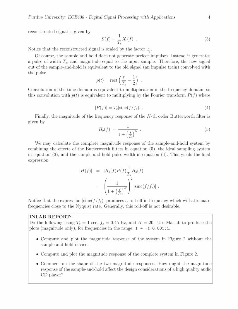
INLAB REPORT:

Do the following using Ts = 1 sec, fc = 0.45 Hz, and N = 20. Use Matlab to produce theplots (magnitude only), for frequencies in the range: f = -1:0.001:1.

• Compute and plot the magnitude response of the system in Figure 2 without thesample-and-hold device.

• Compute and plot the magnitude response of the complete system in Figure 2.

• Comment on the shape of the two magnitude responses. How might the magnituderesponse of the sample-and-hold affect the design considerations of a high quality audioCD player?

Purdue University: ECE438 - Digital Signal Processing with Applications 5

2 Simulink Overview

Upsampler

L

Spectrum

Analyzer

Simulink Blocks

Full Block Library

ScopeNetwork

Analyzer

Impulse

Generator

Experiment 3

Discrete Time

Interpolator

Experiment 2

Sampling and Reconstruction

Using a Sample and Hold

Experiment 1

Sampling and Reconstruction

Using an Inpulse Generator

Analog Butterworth

LP Filter1

Figure 3: Simulink utilities for lab 4.

In this lab we will use Simulink to simulate the effects of the sampling and reconstructionprocesses. Simulink treats all signals as continuous-time signals. This means that “sampled”signals are really just continuous-time signals that contain a series of finite-width pulses. Theheight of each of these pulses is the amplitude of the input signal at the beginning of thepulse. In other words, both the sampling action and the zero-order-hold reconstruction aredone at the same time; the discrete-time signal itself is never generated. This means that theimpulse-generator block is really a “pulse-generator”, or zero-order-hold device. Rememberthat, in Simulink, frequency spectra are computed on continuous-time signals. This is whymany aliased components will appear in the spectra.

3 Sampling and Reconstruction with an Impulse Gen-

erator

Help on Simulink

Help on printing figures in SimulinkDown load Lab4Utilities.zip

In this section, we will experiment with the sampling and reconstruction of signals usinga pulse generator. This pulse generator is the combination of an ideal impulse generator anda perfect zero-order-hold device.

In order to run the experiment, first download the required Lab4Utilities . OnceMatlab is started, type “Lab4”. A set of Simulink blocks and experiments will come up as

Purdue University: ECE438 - Digital Signal Processing with Applications 6

shown in Fig 3.

Spectrum

Analyzer

Signal

Generator

ScopeMux

Mux

Impulse

Generator

Figure 4: Simulink model for sampling and reconstruction using an impulse generator.

Before starting this experiment, use the MATLAB command close all to close all figuresother than the Simulink windows. Double click on the icon named Sampling and Reconstruc-

tion Using An Impulse Generator to bring up the first experiment as shown in Figure 4. Inthis experiment, a sine wave is sampled at a frequency of 1 Hz; then the sampled discrete-time signal is used to generate rectangular impulses of duration 0.3 sec and amplitude equalto the sample values. The block named Impulse Generator carries out both the samplingof the sine wave and its reconstruction with pulses. A single Scope is used to plot both theinput and output of the impulse generator, and a Spectrum Analyzer is used to plot theoutput pulse train and its spectrum.

First, run the simulation with the frequency of input sine wave set to 0.1 Hz (initialsetting of the experiment). Let the simulation run until it terminates to get an accurate plotof the output frequencies. Then print the output of Scope and the Spectrum Analyzer. Besure to label your plots.

INLAB REPORT:

Submit the plot of the input/output signals and the plot of the output signal and its frequencyspectrum. On the plot of the spectrum of the reconstructed signal, circle the aliases, i.e. thecomponents that do NOT correspond to the input sine wave.

Ideal impulse functions can only be approximated. In the initial setup, the pulse widthis 0.3 sec, which is less then the sampling period of 1 sec. Try setting the pulse width to0.1 sec and run the simulation. Print the output of the Spectrum Analyzer.

INLAB REPORT:

Submit the plot of the output frequency spectrum for a pulse width of 0.1 sec. Indicate onyour plot what has changed and explain why.

Set the pulse width back to 0.3 sec and change the frequency of the sine wave to 0.8 Hz.Run the simulation and print the output of the Scope and the Spectrum Analyzer.

Purdue University: ECE438 - Digital Signal Processing with Applications 7

Scope4Scope3Scope2Scope1

Sample−and−Hold

Network

Analyzer

Analog Butterworth

LP Filter1

Analog Butterworth

LP Filter 2

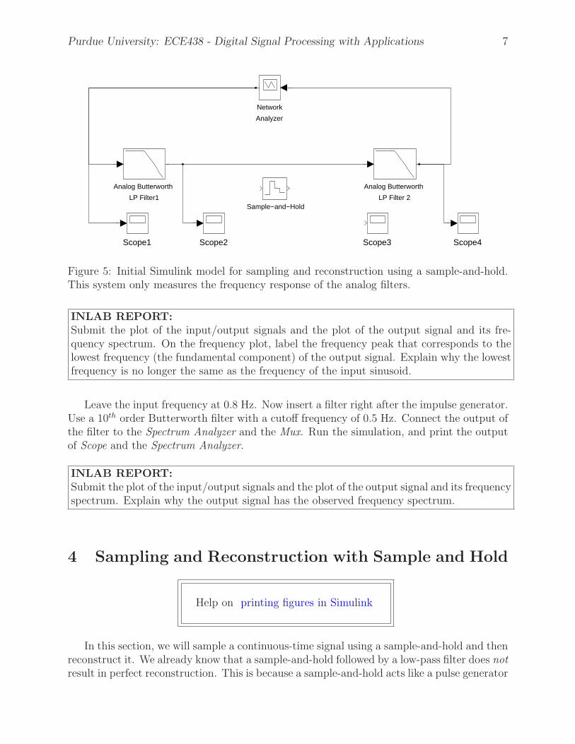
Figure 5: Initial Simulink model for sampling and reconstruction using a sample-and-hold.This system only measures the frequency response of the analog filters.

INLAB REPORT:

Submit the plot of the input/output signals and the plot of the output signal and its fre-quency spectrum. On the frequency plot, label the frequency peak that corresponds to thelowest frequency (the fundamental component) of the output signal. Explain why the lowestfrequency is no longer the same as the frequency of the input sinusoid.

Leave the input frequency at 0.8 Hz. Now insert a filter right after the impulse generator.Use a 10th order Butterworth filter with a cutoff frequency of 0.5 Hz. Connect the output ofthe filter to the Spectrum Analyzer and the Mux. Run the simulation, and print the outputof Scope and the Spectrum Analyzer.

INLAB REPORT:

Submit the plot of the input/output signals and the plot of the output signal and its frequencyspectrum. Explain why the output signal has the observed frequency spectrum.

4 Sampling and Reconstruction with Sample and Hold

Help on printing figures in Simulink

In this section, we will sample a continuous-time signal using a sample-and-hold and thenreconstruct it. We already know that a sample-and-hold followed by a low-pass filter does not

result in perfect reconstruction. This is because a sample-and-hold acts like a pulse generator

Purdue University: ECE438 - Digital Signal Processing with Applications 8

with a pulse duration of one sampling period. This “pulse shape” of the sample-and-hold iswhat distorts the frequency spectrum (see Sec 1.2).

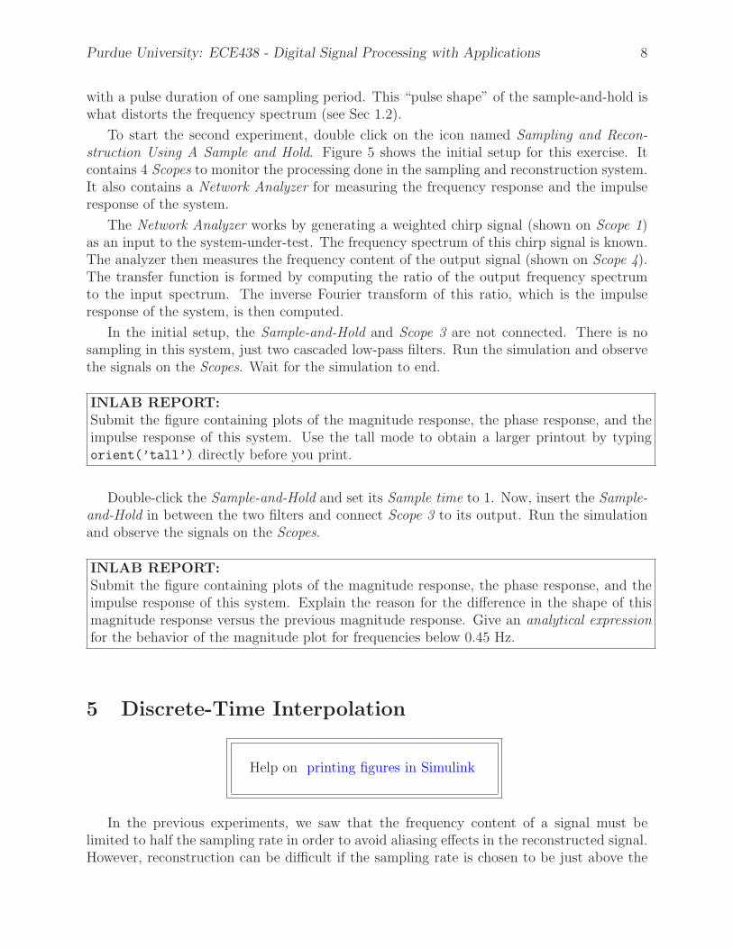
To start the second experiment, double click on the icon named Sampling and Recon-

struction Using A Sample and Hold. Figure 5 shows the initial setup for this exercise. Itcontains 4 Scopes to monitor the processing done in the sampling and reconstruction system.It also contains a Network Analyzer for measuring the frequency response and the impulseresponse of the system.

The Network Analyzer works by generating a weighted chirp signal (shown on Scope 1)as an input to the system-under-test. The frequency spectrum of this chirp signal is known.The analyzer then measures the frequency content of the output signal (shown on Scope 4).The transfer function is formed by computing the ratio of the output frequency spectrumto the input spectrum. The inverse Fourier transform of this ratio, which is the impulseresponse of the system, is then computed.

In the initial setup, the Sample-and-Hold and Scope 3 are not connected. There is nosampling in this system, just two cascaded low-pass filters. Run the simulation and observethe signals on the Scopes. Wait for the simulation to end.

INLAB REPORT:

Submit the figure containing plots of the magnitude response, the phase response, and theimpulse response of this system. Use the tall mode to obtain a larger printout by typingorient(’tall’) directly before you print.

Double-click the Sample-and-Hold and set its Sample time to 1. Now, insert the Sample-

and-Hold in between the two filters and connect Scope 3 to its output. Run the simulationand observe the signals on the Scopes.

INLAB REPORT:

Submit the figure containing plots of the magnitude response, the phase response, and theimpulse response of this system. Explain the reason for the difference in the shape of thismagnitude response versus the previous magnitude response. Give an analytical expression

for the behavior of the magnitude plot for frequencies below 0.45 Hz.

5 Discrete-Time Interpolation

Help on printing figures in Simulink

In the previous experiments, we saw that the frequency content of a signal must belimited to half the sampling rate in order to avoid aliasing effects in the reconstructed signal.However, reconstruction can be difficult if the sampling rate is chosen to be just above the

Purdue University: ECE438 - Digital Signal Processing with Applications 9

signal c

signal bsignal a

Zero−Order

Hold1

Zero−Order

HoldUpsampler

L

Spectrum

Analyzer

Signal

Generator

ScopeMux

Mux

Gain

1

Discrete−time

LP Filter

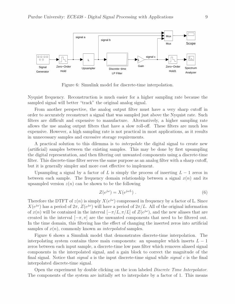
Figure 6: Simulink model for discrete-time interpolation.

Nyquist frequency. Reconstruction is much easier for a higher sampling rate because thesampled signal will better “track” the original analog signal.

From another perspective, the analog output filter must have a very sharp cutoff inorder to accurately reconstruct a signal that was sampled just above the Nyquist rate. Suchfilters are difficult and expensive to manufacture. Alternatively, a higher sampling rateallows the use analog output filters that have a slow roll-off. These filters are much lessexpensive. However, a high sampling rate is not practical in most applications, as it resultsin unnecessary samples and excessive storage requirements.

A practical solution to this dilemma is to interpolate the digital signal to create new(artificial) samples between the existing samples. This may be done by first upsamplingthe digital representation, and then filtering out unwanted components using a discrete-timefilter. This discrete-time filter serves the same purpose as an analog filter with a sharp cutoff,but it is generally simpler and more cost effective to implement.

Upsampling a signal by a factor of L is simply the process of inserting L − 1 zeros inbetween each sample. The frequency domain relationship between a signal x(n) and itsupsampled version z(n) can be shown to be the following

Z(ejω) = X(ejωL) . (6)

Therefore the DTFT of z(n) is simply X(ejω) compressed in frequency by a factor of L. SinceX(ejω) has a period of 2π, Z(ejω) will have a period of 2π/L. All of the original informationof x(n) will be contained in the interval [−π/L, π/L] of Z(ejω), and the new aliases that arecreated in the interval [−π, π] are the unwanted components that need to be filtered out.In the time domain, this filtering has the effect of changing the inserted zeros into artificialsamples of x(n), commonly known as interpolated samples.

Figure 6 shows a Simulink model that demonstrates discrete-time interpolation. Theinterpolating system contains three main components: an upsampler which inserts L − 1zeros between each input sample, a discrete-time low pass filter which removes aliased signalcomponents in the interpolated signal, and a gain block to correct the magnitude of thefinal signal. Notice that signal a is the input discrete-time signal while signal c is the finalinterpolated discrete-time signal.

Open the experiment by double clicking on the icon labeled Discrete Time Interpolator.The components of the system are initially set to interpolate by a factor of 1. This means

Purdue University: ECE438 - Digital Signal Processing with Applications 10

that the input and output signals will be the same except for a delay. Run this model withthe initial settings, and observe the signals on the Scope.

Simulink represents any discrete-time signal by holding each sample value over a certaintime period. This representation is equivalent to a sample-and-hold reconstruction of theunderlying discrete-time signal. Therefore, a continuous-time Spectrum Analyzer may beused to view the frequency content of the output signal c. The Zero-Order Hold at the Gain

output is required as a buffer for the Spectrum Analyzer in order to set its internal samplingperiod.

The lowest frequency component in the spectrum corresponds to the frequency content ofthe original input signal, while the higher frequencies are aliased components resulting fromthe sample-and-hold reconstruction. Notice that the aliased components of signal c appearat multiples of the sampling frequency of 1 Hz. Print the output of the Spectrum Analyzer.

INLAB REPORT:

Submit your plot of signal c and its frequency spectrum. Circle the aliased components inyour plot.

Next modify the system to upsample by a factor of 4 by setting this parameter in theUpsampler. You will also need to set the Sample time of the DT filter to 0.25. This effectivelyincreases the sampling frequency of the system to 4 Hz. Run the simulation again and observethe behavior of the system. Notice that zeros have been inserted between samples of theinput signal. After you get an accurate plot of the output frequency spectrum, print theoutput of the Spectrum Analyzer.

Notice the new aliased components generated by the upsampler. Some of these spectralcomponents lie between the frequency of the original signal and the new sampling frequency,4 Hz. These aliases are due to the zeros that are inserted by the upsampler.

INLAB REPORT:

Submit your plot of signal c and its frequency spectrum. On your frequency plot, circle thefirst aliased component and label the value of its center frequency. Comment on the shapeof the envelope of the spectrum.

Notice in the previous Scope output that the process of upsampling causes a decrease inthe energy of the sample-and-hold representation by a factor of 4. This is the reason forusing the Gain block.

Now determine the gain factor of the Gain block and the cutoff frequency of the Discrete-

time LP filter needed to produce the desired interpolated signal. Run the simulation andobserve the behavior of the system. After you get an accurate plot of the output frequencyspectrum, print the output of the Spectrum Analyzer. Identify the change in the location ofthe aliased components in the output signal.

Purdue University: ECE438 - Digital Signal Processing with Applications 11

INLAB REPORT:

Submit your plot of signal c and its frequency spectrum. Give the values of the cutofffrequency and gain that were used. On your frequency plot, circle the location of the firstaliased component. Explain why discrete-time interpolation is desirable before reconstructinga sampled signal.

6 Discrete-Time Decimation

Down load music.au

How to load and play audio signals

In the previous section, we used interpolation to increase the sampling rate of a discrete-time signal. However, we often have the opposite problem in which the desired samplingrate is lower than the sampling rate of the available data. In this case, we must use a processcalled decimation to reduce the sampling rate of the signal.

Decimating, or downsampling, a signal x(n) by a factor of D is the process of creating anew signal y(n) by taking only every Dth sample of x(n). Therefore y(n) is simply x(Dn).The frequency domain relationship between y(n) and x(n) can be shown to be the following:

Y (ejω) =1

D

D−1∑

k=0

X

(

ω − 2πk

D

)

. (7)

Notice the similarity of (7) to the sampling theorem equation in (1). This similarity shouldbe expected because decimation is the process of sampling a discrete-time signal. In thiscase, Y (ejω) is formed by taking X(ejω) in the interval [−π, π] and expanding it in frequencyby a factor of D. Then it is repeated in frequency every 2π, and scaled in amplitude by 1/D.For similar reasons as described for equation (1), aliasing will be prevented if in the interval[−π, π], X(ejω) is zero outside the interval [−π/D, π/D]. Then (7) simplifies to

Y (ejω) =1

DX(

ej ω

D

)

for ω ∈ [−π, π] . (8)

A system for decimating a signal is shown in Fig. 7. The signal is first filtered using a lowpass filter with a cutoff frequency of π/2 rad/sample. This insures that the signal is bandlimited so that the relationship in (8) holds. The output of the filter is then subsampled byremoving every other sample.

Down load the signal music.au . Read in the signal contained in music.au using auread,and then play it back with sound. The signal contained in music.au was sampled at 16 kHz,so it will sound much too slow when played back at the default 8 kHz sampling rate.

To correct the sampling rate of the signal, form a new signal, sig1, by selecting everyother sample of the music vector. Play the new signal using sound, and listen carefully tothe new signal.

Purdue University: ECE438 - Digital Signal Processing with Applications 12

low pass filterwith cutoff of

ω = π/2

x(n)2

x(1:2:N) y(n)

Figure 7: This system decimates a discrete-time signal by a factor of 2.

Next compute a second subsampled signal, sig2, by first low pass filtering the originalmusic vector using a discrete-time filter of length 20, and with a cutoff frequency of π/2.Then decimate the filtered signal by 2, and listen carefully to the new signal.

Hint: You can filter the signal by using the Matlab command output = conv(s,h),where s is the signal, and h is the impulse response of the desired filter. To design a lengthM low-pass filter with cutoff frequency W rad/sample, use the command h = fir1(M,W/pi).

INLAB REPORT:

Hand in the Matlab code for this exercise. Also, comment on the quality of the audio signalgenerated by using the two decimation methods. Was there any noticeable distortion insig1? If so, describe the distortion.