lab9 - measurement invariance

Lab9 - Measurement InvarianceAdam Garber

Factor Analysis ED 216B - Instructor: Karen Nylund-Gibson

March 30, 2020

Contents

1 Lab 9 - Begin 2

2 Estimate the Unconditional Confirmatory Factor Analysis (CFA) model 3

3 Run separate CFA models for each sub-sample 4

3.1 Group freelnch = 0 (low) CFA . . . . . . . . . . . . . . . . . . . . . . . . . . . . . . . . . . . 4

3.2 Group freelnch = 1 (moderate to high) CFA . . . . . . . . . . . . . . . . . . . . . . . . . . . . 5

4 ~~~~~~~~~ Multi-Group Invariance Models ~~~~~~~~~ 6

4.1 Configural invariance . . . . . . . . . . . . . . . . . . . . . . . . . . . . . . . . . . . . . . . . . 6

4.2 Metric invariance . . . . . . . . . . . . . . . . . . . . . . . . . . . . . . . . . . . . . . . . . . . 7

4.3 Scalar invariance . . . . . . . . . . . . . . . . . . . . . . . . . . . . . . . . . . . . . . . . . . . 9

4.4 Strict invariance . . . . . . . . . . . . . . . . . . . . . . . . . . . . . . . . . . . . . . . . . . . 10

4.5 Structural invariance A (fixed factor variances) . . . . . . . . . . . . . . . . . . . . . . . . . . 11

4.6 Structural invariance B (fixed factor variances and equal covariances) . . . . . . . . . . . . . . 12

4.7 Latent Factor Means differences: . . . . . . . . . . . . . . . . . . . . . . . . . . . . . . . . . . 13

5 Comparing Fit Across Models 14

5.1 Guidlines: for loadings & fit indices . . . . . . . . . . . . . . . . . . . . . . . . . . . . . . . . . 14

5.2 Calculate Satora-Bentler scaled Chi-square difference test (use with MLR estimator) . . . . . 15

5.3 Invariance short-cut . . . . . . . . . . . . . . . . . . . . . . . . . . . . . . . . . . . . . . . . . 16

5.4 Invariance Testing (Chi-square values - Chi-Square difference p-values are biased) . . . . . . . 16

5.5 End of Lab 9 . . . . . . . . . . . . . . . . . . . . . . . . . . . . . . . . . . . . . . . . . . . . . 17

1

6 References 17

DATA SOURCE: This lab exercise utilizes the NCES public-use dataset: Education Longitudinal Study of2002 (Lauff & Ingels, 2014) See website: nces.ed.gov

# load packageslibrary(MplusAutomation)library(haven)library(rhdf5)library(tidyverse)library(here)library(corrplot)library(kableExtra)library(reshape2)library(semPlot)

1 Lab 9 - Begin

Read in data

lab_data <- read_csv(here("data", "els_sub5_data.csv"))

Preparations: subset,reorder, rename, and recode data

invar_data <- lab_data %>%select(bystlang, freelnch, byincome, # covariates

stolen, t_hurt, p_fight, hit, damaged, bullied, # factor 1 (indicators)safe, disrupt, gangs, rac_fght, # factor 2 (indicators)late, skipped, mth_read, mth_test, rd_test) %>%

rename("unsafe" = "safe") %>%mutate(

freelnch = case_when( # Grade 10, percent free lunch - transform to binaryfreelnch < 3 ~ 0, # school has less than 11%freelnch >= 3 ~ 1)) # school has greater than or equal to 11%

table(invar_data$freelnch) # reasonably balanced groups

Take a quick look at variable distributions

melt(invar_data[,4:13]) %>%ggplot(., aes(x=value, label=variable)) +geom_histogram(bins = 15) +facet_wrap(~variable, scales = "free")

Reverse code factor for ease of interpretation

2

https://nces.ed.gov/surveys/els2002/avail_data.asp

cols = c("unsafe", "disrupt", "gangs", "rac_fght")

invar_data[ ,cols] <- 5 - invar_data[ ,cols]

Factor names and interpretation:

• VICTIM: student reports being a victim of injury to self or property– scale range: Never, Once or twice, More than twice– higher values indicate greater frequency of victimization events

• NEG_CLIM: Student reports on negative school climate attributes– scale range: Strongly Disagree - Strongly Agree– higher values indicate a more negative climate

Check correct coding, explore correlations

cor_matrix <- cor(invar_data[4:13], use = "pairwise.complete.obs")

corrplot(cor_matrix,method = "circle",type = "upper")

2 Estimate the Unconditional Confirmatory Factor Analysis(CFA) model

Number of parameters = 31

• 10 item loadings• 10 intercepts• 10 residual variances• 01 factor co-variances

cfa_m0 <- mplusObject(TITLE = "model0 - unconditional CFA model",VARIABLE =

"usevar = stolen-rac_fght;",

ANALYSIS ="estimator = mlr;",

MODEL ="VICTIM by stolen* t_hurt p_fight hit damaged bullied;VICTIM@1; ! UVI identification

NEG_CLIM by unsafe* disrupt gangs rac_fght;

3

NEG_CLIM@1; ",

PLOT = "type = plot3;",OUTPUT = "sampstat standardized residual modindices (3.84);",

usevariables = colnames(invar_data),rdata = invar_data)

cfa_m0_fit <- mplusModeler(cfa_m0,dataout=here("invar_mplus", "lab9_invar_data.dat"),modelout=here("invar_mplus", "M0_CFA_fullsample.inp"),check=TRUE, run = TRUE, hashfilename = FALSE)

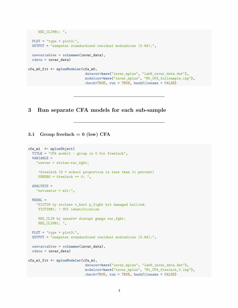
3 Run separate CFA models for each sub-sample

3.1 Group freelnch = 0 (low) CFA

cfa_m1 <- mplusObject(TITLE = "CFA model1 - group is 0 for freelnch",VARIABLE =

"usevar = stolen-rac_fght;

!freelnch (0 = school proportion is less than 11 percent)USEOBS = freelnch == 0; ",



NEG_CLIM by unsafe* disrupt gangs rac_fght;NEG_CLIM@1; ",



cfa_m1_fit <- mplusModeler(cfa_m1,dataout=here("invar_mplus", "lab9_invar_data.dat"),modelout=here("invar_mplus", "M1_CFA_freelnch_0.inp"),check=TRUE, run = TRUE, hashfilename = FALSE)

4

3.2 Group freelnch = 1 (moderate to high) CFA

cfa_m2 <- mplusObject(TITLE = "CFA model2 - group is 1 for freelnch",VARIABLE =


!freelnch (1 = school proportion is greater than or equal to 11 percent)USEOBS = freelnch == 1; ",



NEG_CLIM by unsafe* disrupt gangs rac_fght;NEG_CLIM@1; ",



cfa_m2_fit <- mplusModeler(cfa_m2,dataout=here("invar_mplus", "lab9_invar_data.dat"),modelout=here("invar_mplus", "M2_CFA_freelnch_1.inp"),check=TRUE, run = TRUE, hashfilename = FALSE)

5

4 ~~~~~~~~~ Multi-Group Invariance Models ~~~~~~~~~

Figure: Picture depicting mean structure from slide by Dr. Karen Nylund-Gibson

4.1 Configural invariance

• free item loadings, intercepts, and residuals• factor means fixed to zero• factor variances fixed to 1


• 20 item loadings (10items*2groups)• 20 intercepts• 20 residual variances• 02 factor co-variances (1 for each group)

cfa_m3 <- mplusObject(TITLE = "CFA model3 - configural invariance",VARIABLE =


6

grouping = freelnch (0=freelnch_0 1=freelnch_1); ",



NEG_CLIM by unsafe* disrupt gangs rac_fght;NEG_CLIM@1;

[VICTIM-NEG_CLIM@0]; !factor means set to zero

MODEL freelnch_1:

VICTIM by stolen* t_hurt p_fight hit damaged bullied;VICTIM@1;

[stolen t_hurt p_fight hit damaged bullied]; !free intercepts


[unsafe disrupt gangs rac_fght]; !free intercepts

[VICTIM-NEG_CLIM@0]; ",



cfa_m3_fit <- mplusModeler(cfa_m3,dataout=here("invar_mplus", "lab9_invar_data.dat"),modelout=here("invar_mplus", "M3_configural.inp"),check=TRUE, run = TRUE, hashfilename = FALSE)

4.2 Metric invariance

• item loadings (set to equal)• free intercepts and residuals• factor means fixed to zero• free factor variances in group 2


7

• 10 item loadings (set to equal)• 20 intercepts• 20 residual variances• 02 factor variances• 02 factor co-variances

cfa_m4 <- mplusObject(TITLE = "CFA model4 - metric invariance",VARIABLE =






[VICTIM-NEG_CLIM@0];

MODEL freelnch_1:

VICTIM; ! free factor variances for group 2

[stolen t_hurt p_fight hit damaged bullied];

NEG_CLIM;

[unsafe disrupt gangs rac_fght];

[VICTIM-NEG_CLIM@0]; ",



cfa_m4_fit <- mplusModeler(cfa_m4,dataout=here("invar_mplus", "lab9_invar_data.dat"),modelout=here("invar_mplus", "M4_metric.inp"),check=TRUE, run = TRUE, hashfilename = FALSE)

8

4.3 Scalar invariance

• item loadings (set to equal)• intercepts (set to equal)• free residuals• free factor variances and means in group 2


• 10 item loadings (set to equal)• 10 intercepts (set to equal)• 20 residual variances• 02 factor variances• 02 factor co-variances• 02 factor means

cfa_m5 <- mplusObject(TITLE = "model5 - scalar invariance",VARIABLE =




MODEL ="VICTIM by stolen* t_hurt p_fight hit damaged bullied;VICTIM@1;



MODEL freelnch_1:


NEG_CLIM;

[VICTIM-NEG_CLIM]; ! free factor means",



9

cfa_m5_fit <- mplusModeler(cfa_m5,dataout=here("invar_mplus", "lab9_invar_data.dat"),modelout=here("invar_mplus", "M5_scalar.inp"),check=TRUE, run = TRUE, hashfilename = FALSE)

4.4 Strict invariance

• item loadings (set to equal)• intercepts (set to equal)• residuals (set to equal)• free factor variances and means in group 2



cfa_m6 <- mplusObject(TITLE = "model6 - strict invariance",VARIABLE =







stolen-rac_fght(1-10); ! set residuals to be equal across groups

MODEL freelnch_1:


10

NEG_CLIM;

[VICTIM-NEG_CLIM]; ! free factor means

stolen-rac_fght(1-10); ",



cfa_m6_fit <- mplusModeler(cfa_m6,dataout=here("invar_mplus", "lab9_invar_data.dat"),modelout=here("invar_mplus", "M6_strict.inp"),check=TRUE, run = TRUE, hashfilename = FALSE)

4.5 Structural invariance A (fixed factor variances)

Demonstration of structural invariance using the Scalar model

• item loadings (set to equal)• intercepts (set to equal)• free residuals (Scalar)• factor means free in group 2• factor variances (set to 1)• free factor covariances



# fixed factor variancescfa_m7 <- mplusObject(

TITLE = "model7 - structural invariance A" ,VARIABLE =



11





MODEL freelnch_1:


VICTIM@1; NEG_CLIM@1; ! fix factor variance to 1",



cfa_m7_fit <- mplusModeler(cfa_m7,dataout=here("invar_mplus", "lab9_invar_data.dat"),modelout=here("invar_mplus", "M7_structuralA.inp"),check=TRUE, run = TRUE, hashfilename = FALSE)

4.6 Structural invariance B (fixed factor variances and equal covariances)

Demonstration of structural invariance using the Scalar model

• item loadings (set to equal)• intercepts (set to equal)• free residuals (Scalar)• factor means free in group 2• factor variances (set to equal)• factor covariances (set to equal)


• 10 item loadings (set to equal)• 10 intercepts (set to equal)• 20 residual variances• 00 factor variances• 01 factor co-variances

12

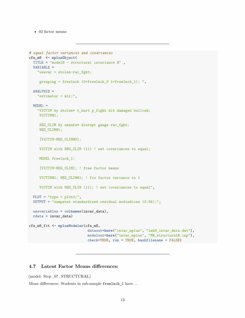
• 02 factor means

# equal factor variances and covariancescfa_m8 <- mplusObject(

TITLE = "model8 - structural invariance B" ,VARIABLE =







VICTIM with NEG_CLIM (11) ! set covariances to equal;

MODEL freelnch_1:


VICTIM@1; NEG_CLIM@1; ! fix factor variance to 1

VICTIM with NEG_CLIM (11); ! set covariances to equal",



cfa_m8_fit <- mplusModeler(cfa_m8,dataout=here("invar_mplus", "lab9_invar_data.dat"),modelout=here("invar_mplus", "M8_structuralB.inp"),check=TRUE, run = TRUE, hashfilename = FALSE)

4.7 Latent Factor Means differences:

(model: Step_07_STRUCTURAL)

Mean differences: Students in sub-sample freelnch_1 have. . .

13

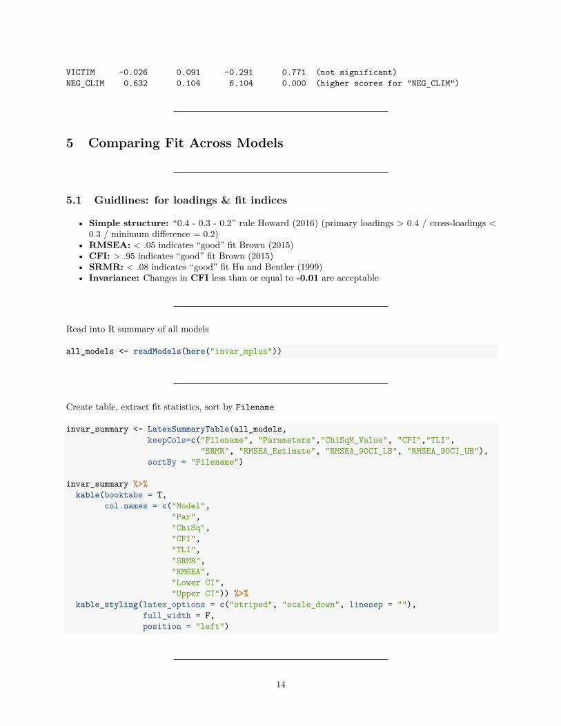
VICTIM -0.026 0.091 -0.291 0.771 (not significant)NEG_CLIM 0.632 0.104 6.104 0.000 (higher scores for "NEG_CLIM")

5 Comparing Fit Across Models

5.1 Guidlines: for loadings & fit indices

• Simple structure: “0.4 - 0.3 - 0.2” rule Howard (2016) (primary loadings > 0.4 / cross-loadings <0.3 / minimum difference = 0.2)

• RMSEA: < .05 indicates “good” fit Brown (2015)• CFI: > .95 indicates “good” fit Brown (2015)• SRMR: < .08 indicates “good” fit Hu and Bentler (1999)• Invariance: Changes in CFI less than or equal to -0.01 are acceptable

Read into R summary of all models

all_models <- readModels(here("invar_mplus"))

Create table, extract fit statistics, sort by Filename

invar_summary <- LatexSummaryTable(all_models,keepCols=c("Filename", "Parameters","ChiSqM_Value", "CFI","TLI",

"SRMR", "RMSEA_Estimate", "RMSEA_90CI_LB", "RMSEA_90CI_UB"),sortBy = "Filename")

invar_summary %>%kable(booktabs = T,

col.names = c("Model","Par","ChiSq","CFI","TLI","SRMR","RMSEA","Lower CI","Upper CI")) %>%

kable_styling(latex_options = c("striped", "scale_down", linesep = ""),full_width = F,position = "left")

14

5.2 Calculate Satora-Bentler scaled Chi-square difference test (use with MLRestimator)

See website: stats.idre.ucla.edu

• SB0 = null model Chi-square value• SB1 = alternate model Chi-square value• c0 = null model scaling correction factor• c1 = alternate model scaling correction factor• d0 = null model degrees of freedom• d1 = alternate model degrees of freedom• df = Chi-square test degrees of freedom

compare configural to metric

SB0 <- all_models[["M4_metric.out"]][["summaries"]][["ChiSqM_Value"]]SB1 <- all_models[["M3_configural.out"]][["summaries"]][["ChiSqM_Value"]]c0 <- all_models[["M4_metric.out"]][["summaries"]][["ChiSqM_ScalingCorrection"]]c1 <- all_models[["M3_configural.out"]][["summaries"]][["ChiSqM_ScalingCorrection"]]d0 <- all_models[["M4_metric.out"]][["summaries"]][["ChiSqM_DF"]]d1 <- all_models[["M3_configural.out"]][["summaries"]][["ChiSqM_DF"]]df <- abs(d0-d1)

# Satora-Bentler scaled Difference test equationscd <- (((d0*c0)-(d1*c1))/(d0-d1))t <- (((SB0*c0)-(SB1*c1))/(cd))

# Chi-square and degrees of freedomtdf

# Significance testpchisq(t, df, lower.tail=FALSE)

compare metric to scalar

SB0 <- all_models[["M5_scalar.out"]][["summaries"]][["ChiSqM_Value"]]SB1 <- all_models[["M4_metric.out"]][["summaries"]][["ChiSqM_Value"]]c0 <- all_models[["M5_scalar.out"]][["summaries"]][["ChiSqM_ScalingCorrection"]]c1 <- all_models[["M4_metric.out"]][["summaries"]][["ChiSqM_ScalingCorrection"]]d0 <- all_models[["M5_scalar.out"]][["summaries"]][["ChiSqM_DF"]]d1 <- all_models[["M4_metric.out"]][["summaries"]][["ChiSqM_DF"]]df <- abs(d0-d1)

# Satora-Bentler scaled Difference test equationscd <- (((d0*c0)-(d1*c1))/(d0-d1))t <- (((SB0*c0)-(SB1*c1))/(cd))

15

https://stats.idre.ucla.edu/mplus/faq/how-can-i-compute-a-chi-square-test-for-nested-models-with-the-mlr-or-mlm-estimators/

# Chi-square and degrees of freedomtdf

# Significance testpchisq(t, df, lower.tail=FALSE)

5.3 Invariance short-cut

mx <- mplusObject(TITLE = "INVARIANCE SHORT_CUT - LAB 9 DEMO",VARIABLE =



ANALYSIS ="Estimator = MLR;MODEL= CONFIG METRIC SCALAR;",


NEG_CLIM by unsafe* disrupt gangs rac_fght;NEG_CLIM@1;" ,

PLOT = "",OUTPUT = "sampstat residual;",


mx_fit <- mplusModeler(mx,dataout=here("invar_short", "Invar_short_cut.dat"),modelout=here("invar_short", "Invar_short_cut.inp"),check=TRUE, run = TRUE, hashfilename = FALSE)

5.4 Invariance Testing (Chi-square values - Chi-Square difference p-values arebiased)

Number of Degrees ofModel Parameters Chi-Square Freedom P-Value

Configural 62 149.315 68 0.0000Metric 54 163.312 76 0.0000

16

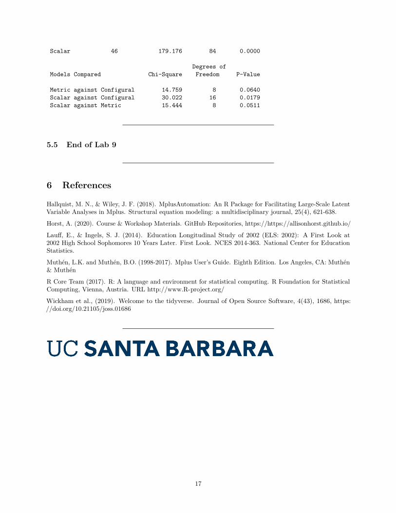
Scalar 46 179.176 84 0.0000

Degrees ofModels Compared Chi-Square Freedom P-Value

Metric against Configural 14.759 8 0.0640Scalar against Configural 30.022 16 0.0179Scalar against Metric 15.444 8 0.0511

5.5 End of Lab 9

6 References

Hallquist, M. N., & Wiley, J. F. (2018). MplusAutomation: An R Package for Facilitating Large-Scale LatentVariable Analyses in Mplus. Structural equation modeling: a multidisciplinary journal, 25(4), 621-638.

Horst, A. (2020). Course & Workshop Materials. GitHub Repositories, https://https://allisonhorst.github.io/

Lauff, E., & Ingels, S. J. (2014). Education Longitudinal Study of 2002 (ELS: 2002): A First Look at2002 High School Sophomores 10 Years Later. First Look. NCES 2014-363. National Center for EducationStatistics.

Muthén, L.K. and Muthén, B.O. (1998-2017). Mplus User’s Guide. Eighth Edition. Los Angeles, CA: Muthén& Muthén

R Core Team (2017). R: A language and environment for statistical computing. R Foundation for StatisticalComputing, Vienna, Austria. URL http://www.R-project.org/

Wickham et al., (2019). Welcome to the tidyverse. Journal of Open Source Software, 4(43), 1686, https://doi.org/10.21105/joss.01686

17

https://https://allisonhorst.github.io/

http://www.R-project.org/

https://doi.org/10.21105/joss.01686

https://doi.org/10.21105/joss.01686

lab9 - measurement invariance

Documents