labor 14.661. 11-13: matching and unemployment · daron acemoglu (mit) search, matching,...

Labor Economics, 14.661. Lectures 11-13: Search, Matching and Unemployment

Daron Acemoglu

MIT

December 5, 7 and 12, 2017.

Daron Acemoglu (MIT) Search, Matching, Unemployment December 5, 7 and 12, 2017. 1 / 104

Introduction Introduction

Introduction

Central question for labor and macro: what determines the level of employment and unemployment in the economy?

Textbook answer: labor supply, labor demand, and unemployment as “leisure”.

Neither realistic nor a useful framework for analysis.

Alternative: labor market frictions

Related questions raised by the presence of frictions:

is the level of employment effi cient/optimal? how is the composition and quality of jobs determined, is it effi cient? distribution of earnings across workers.



Introduction (continued)

Applied questions:

why was unemployment around 4-5% in the US economy until the 1970s? why did the increase in the 70s and 80s, and then decline again in the late 90s? why did it then remain high throughout the 90s and 2000s? why did European unemployment increase in the 1970s and remain persistently high? is the unemployment rate the relevant variable to focus on? Or the labor force participation rate? Or the non-employment rate? why is the composition of employment so different across countries?

male versus female, young versus old, high versus low wages



Introduction (continued)

Challenge: how should labor market frictions be modeled?

Alternatives:

incentive problems, effi ciency wages wage rigidities, bargaining, non-market clearing prices search

Search and matching: costly process of workers finding the “right” jobs.

Theoretical interest: how do markets function without the Walrasian auctioneer?

Empirically important,

But how to develop a tractable and rich model?


McCall Model McCall Sequential Search Model

McCall Partial Equilibrium Search Model

The simplest model of search frictions.

Problem of an individual getting draws from a given wage distribution

Decision: which jobs to accept and when to start work.

Jobs sampled sequentially.

Alternative: Stigler, fixed sample search (choose a sample of n jobs and then take the most attractive one).

Sequential search typically more reasonable.

Moreover, whenever sequential search is possible, is preferred to fixed sample search (why?).



∞

∑

Environment

Risk neutral individual in discrete time. At time t = 0, this individual has preferences given by

βt ct t=0

ct =consumption. Start as unemployed, with consumption equal to b All jobs are identical except for their wages, and wages are given by an exogenous stationary distribution of

F (w )

with finite (bounded) support W. At every date, the individual samples a wage wt ∈ W , and has to decide whether to take this or continue searching. Jobs are for life. Draws from W over time are independent and identically distributed.



Environment (continued)

Undirected search, in the sense that the individual has no ability to seek or direct his search towards different parts of the wage distribution (or towards different types of jobs).

Alternative: directed search.



Environment (continued)

Suppose search without recall.

If the worker accepts a job with wage wt , he will be employed at that job forever, so the net present value of accepting a job of wage wt is

wt .

1 − β

Class of decision rules of the agent:

at : W → [0, 1]

as acceptance decision (acceptance probability)



Dynamic Programming Formulation

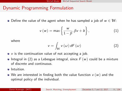
Define the value of the agent when he has sampled a job of w ∈ W: � �

v (w ) = max w

, βv + b1 − β

, (1)

where Z v = v (ω) dF (ω) (2)

W

v is the continuation value of not accepting a job.

Integral in (2) as a Lebesgue integral, since F (w ) could be a mixture of discrete and continuous.

Intuition.

We are interested in finding both the value function v (w ) and the optimal policy of the individual.



Dynamic Programming Formulation (continued)

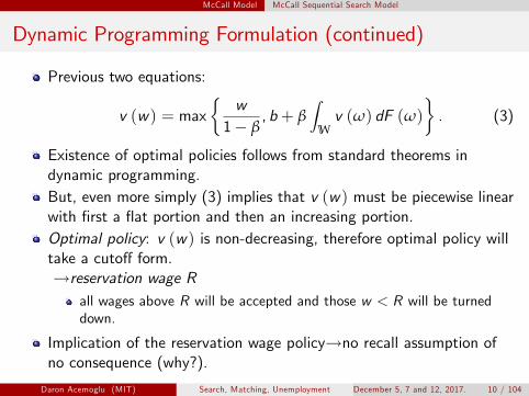
Previous two equations: � �Z w v (w ) = max , b + β v (ω) dF (ω) . (3)

1 − β W

Existence of optimal policies follows from standard theorems in dynamic programming. But, even more simply (3) implies that v (w ) must be piecewise linear with first a flat portion and then an increasing portion. Optimal policy: v (w ) is non-decreasing, therefore optimal policy will take a cutoff form. →reservation wage R

all wages above R will be accepted and those w < R will be turned down.

Implication of the reservation wage policy→no recall assumption of no consequence (why?).



Reservation Wage

Reservation wage given by ZR = b + β v (ω) dF (ω) . (4)

1 − β W

Intuition? Since w < R are turned down, for all w < R Z

v (w ) = b + β v (ω) dF (ω) W

R = ,

1 − β

and for all w ≥ R, w

v (w ) = 1 − β

Therefore, Z RF (R) Z w

v (ω) dF (ω) = + dF (w ) . W 1 − β w ≥R 1 − β


Zw≥R

w1− β

dF (w)�


Reservation Wage (continued)

Combining this with (4), we have � � R RF (R)

Z w = b + β + dF (w )

1 − β 1 − β w ≥R 1 − β

Rewriting Z Z �ZR R RdF (w )+ dF (w ) = b + β dF (w ) +

w <R 1 − β w ≥R 1 − β w <R 1 − β R R Subtracting βR dF (w ) / (1 − β) + βR dF (w ) / (1 − β)w ≥R w <R from both sides, Z ZR R

dF (w ) + dF (w ) w <R 1 − β w ≥R 1 − β Z ZR R −β dF (w ) − β dF (w )

w ≥R 1 − β w <R 1 − β �Z � w − R

= b + β dF (w ) w ≥R 1 − β




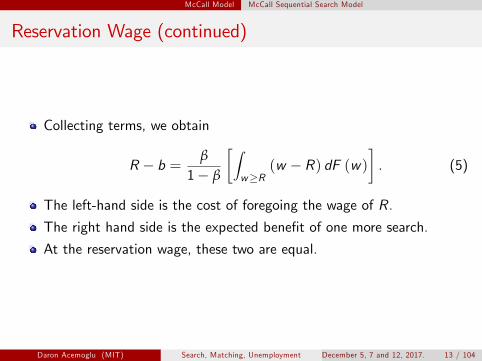
Collecting terms, we obtain �Z � β

R − b = (w − R) dF (w ) . (5)1 − β w ≥R

The left-hand side is the cost of foregoing the wage of R.

The right hand side is the expected benefit of one more search.

At the reservation wage, these two are equal.


Intuition?



Let us define the right hand side of equation (5) as �Z � β

g (R) ≡ (w − R) dF (w ) ,1 − β w ≥R

This is the expected benefit of one more search as a function of the reservation wage. Differentiating �Z �

β β g 0 (R) = − (R − R) f (R) − dF (w )

1 − β 1 − β w ≥R

β = − [1 − F (R)] < 0

1 − β

Therefore equation (5) has a unique solution. Moreover, by the implicit function theorem,

dR 1 = > 0.

db 1 − g 0 (R)




Suppose that the density of F (R), denoted by f (R), exists (was this necessary until now?).

Then the second derivative of g also exists and is

β00 (R) =g f (R) ≥ 0.1 − β

This implies the right hand side of equation (5) is also convex.

What does this mean?


(w)�


Wage Dispersion and Search

Start with equation (5), which is �Z � β

R − b = (w − R) dF (w ) .1 − β w ≥R

Rewrite this as

R − b =

=

�Z � �Z β β

(w − R) dF (w ) + (w − R) dF1 − β w ≥R 1 − β w ≤R�Z �

β − (w − R) dF (w ) ,1 − β w ≤R �Z � β β

(Ew − R) − (w − R) dF (w ) ,1 − β 1 − β w ≤R

where Z Ew = wdF (w )

W

is the mean of the distribution. Daron Acemoglu (MIT) Search, Matching, Unemployment December 5, 7 and 12, 2017. 16 / 104


Wage Dispersion and Search (continued)

Rearranging the previous equation Z R − b = β (Ew − b) − β (w − R) dF (w ) .

w ≤R

Applying integration by parts to the integral on the right hand side, i.e., noting that Z Z R

wdF (w ) = wdF (w ) w ≤R 0 Z R

R = wF (w )| − F (w ) dw0 0 Z R

= RF (R) − F (w ) dw . 0

We obtain Z R R − b = β (Ew − b) + β F (w ) dw . (6)

0



Wage Dispersion and Search (continued)

Now consider a shift from F to F corresponding to a mean preserving spread.

This implies that Ew is unchanged

But by definition of a mean preserving spread (second-order stochastic dominance), the last integral increases.

Therefore, the mean preserving spread induces a shift in the reservation wage from R to R > R.

Intuition?

Relation to the convexity of v (w )?


Unemployment with Sequential Search Unemployment with Sequential Search

Unemployment with Sequential Search

Suppose that there is now a continuum 1 of identical individuals sampling jobs from the same stationary distribution F .

Once a job is created, it lasts until the worker dies, which happens with probability s.

There is a mass of s workers born every period, so that population is constant

New workers start out as unemployed.

The death probability means that the effective discount factor of workers is equal to β (1 − s).

Consequently, the value of having accepted a wage of w is:

w va (w ) = .

1 − β (1 − s)



Unemployment with Sequential Search (continued)

With the same reasoning as before, the value of having a job offer at wage w at hand is

v (w ) = max {va (w ) , b + β (1 − s) v }

with Z v = v (w ) dF .

W

Therefore, the reservation wages given by �Z � β (1 − s)

R − b = (w − R) dF (w ) .1 − β (1 − s) w ≥R



Law of Motion of Unemployment

Let us start time t with Ut unemployed workers.

There will be s new workers born into the unemployment pool.

Out of the Ut unemployed workers, those who survive and do not find a job will remain unemployed.

Therefore Ut+1 = s + (1 − s) F (R)Ut .

Here F (R) is the probability of not finding a job, so (1 − s) F (R) is the joint probability of not finding a job and surviving.

Simple first-order linear difference equation (only depending on the reservation wage R, which is itself independent of the level of unemployment, Ut ).

Since (1 − s) F (R) < 1, it is asymptotically stable, and will converge to a unique steady-state level of unemployment.



Flow Approached Unemployment

This gives us the simplest version of the flow approach to unemployment.

Subtracting Ut from both sides:

Ut+1 − Ut = s (1 − Ut ) − (1 − s) (1 − F (R)) Ut .

If period length is arbitrary, this can be written as

Ut+Δt − Ut = s (1 − Ut ) Δt − (1 − s) (1 − F (R)) Ut Δt + o (Δt) .

Dividing by Δt and taking limits as Δt → 0, we obtain the continuous time version

Ut = s (1 − Ut ) − (1 − s) (1 − F (R)) Ut .



Flow Approached Unemployment (continued)

The unique steady-state unemployment rate where Ut+1 = Ut (or Ut = 0) given by

sU = .

s + (1 − s) (1 − F (R))

Canonical formula of the flow approach.

The steady-state unemployment rate is equal to the job destruction rate (here the rate at which workers die, s) divided by the job destruction rate plus the job creation rate (here in fact the rate at which workers leave unemployment, which is different from the job creation rate).

Clearly, an increases in s will raise steady-state unemployment.

Moreover, an increase in R, that is, a higher reservation wage, will also depress job creation and increase unemployment.


Paradoxes of Search Paradoxes of Search

Paradoxes of Search

The search framework is attractive especially when we want to think of a world without a Walrasian auctioneer, or alternatively a world with “frictions”.

Search theory holds the promise of potentially answering these questions, and providing us with a framework for analysis.

But...



The Rothschild Critique

The key ingredient of the McCall model is non-degenerate wage distribution F (w ).

Where does this come from?

Presumably somebody is offering every wage in the support of this distribution.

Wage posting by firms.

The basis of the Rothschild critique is that it is diffi cult to rationalize the distribution function F (w ) as resulting from profit-maximizing choices of firms.



The Rothschild Critique (continued)

Imagine that the economy consists of a mass 1 of identical workers similar to our searching agent.

On the other side, there are N firms that can productively employ workers. Imagine that firm j has access to a technology such that it can employ lj workers to produce

yj = xj lj

units of output (with its price normalized to one as the numeraire, so that w is the real wage).

Suppose that each firm can only attract workers by posting a single vacancy.

Moreover, to simplify the discussion, suppose that firms post a vacancy at the beginning of the game at t = 0, and then do not change the wage from then on. (why is this useful?)



The Rothschild Critique (continued)

Suppose that the distribution of x in the population of firms is given by G (x) with support X ⊂ R+.

Also assume that there is some cost γ > 0 of posting a vacancy at the beginning, and finally, that N >> 1 (i.e., R ∞N = −∞ dG (x) >> 1) and each worker samples one firm from the distribution of posting firms.

As before, suppose that once a worker accepts a job, this is permanent, and he will be employed at this job forever.

Moreover let us set b = 0, so that there is no unemployment benefits.

Finally, to keep the environment entirely stationary, assume that once a worker accepts a job, a new worker is born, and starts search.

Will these firms offer a non-degenerate wage distribution F (w )?


Theorem

(Rothschild Paradox) When all workers are homogeneous and engage inundirected search, all equilibrium distributions will have a mass point attheir reservation wage R.

w R, and there is no distribution and no search.


Equilibrium Wage Distribution?

The answer is no. Previous analysis: all workers will use a reservation wage, so

a (w ) = 1 if w ≥ R

= 0 otherwise

Since all workers are identical and the equation above determining the reservation wage, (5), has a unique solution, all workers will all be using the same reservation rule, accepting all wages w ≥ R and turning down those w < R. Workers’strategies are therefore again characterized by a reservation wage R. Next consider a firm offering a wage w < R. This wage will be rejected by all workers, and the firm would lose the cost of posting a vacancy. Therefore, in equilibrium when workers use the reservation wage rule of accepting only wages greater than R, all firms will offer the same

Daron Acemoglu age (MIT) Search, Matching, Unemployment December 5, 7 and 12, 2017. 28 / 104

Paradoxes of Search The Diamond Paradox

The Diamond Paradox

In fact, the paradox is even deeper.

Theorem

(Diamond Paradox) For all β < 1, the unique equilibrium in the above economy is R = 0, and all workers accept the first wage offer.

Sketch proof: suppose R ≥ 0, and β < 1.

The optimal acceptance decision for to worker is

a (w ) = 1 if w ≥ R

= 0 otherwise

Therefore, all firms offering w = R is an equilibrium

But also...



The Diamond Paradox (continued)

Lemma There exists ε > 0 such that when “almost all” firms are offering w = R, it is optimal for each worker to use the following acceptance strategy:

a (w ) = 1 if w ≥ max{R − ε, 0} = 0 otherwise

So for any R > 0, a firm can undercut the offers of all other firms and still have its offer accepted.




Sketch proof:

If the worker accepts the wage of R − ε,

R − εaccept u = 1 − β

If he rejects and waits until next period, then since “almost all” firms are offering R,

βRreject u = 1 − β

For all β < 1, there exists ε > 0 such that

accept reject u > u .




Implication: starting from an allocation where all firms offer R, any firm can deviate and offer a wage of R − ε and increase its profits.

This proves that no wage R > 0 can be the equilibrium, proving the proposition.

Is the same true for Nash equilibria?



Solutions to the Diamond Paradox

1

2

3

How do we resolve this paradox?

By assumption: assume that F (w ) is not the distribution of wages, but the distribution of “fruits” exogenously offered by “trees”. This is clearly unsatisfactory, both from the modeling point of view, and from the point of view of asking policy questions from the model (e.g., how does unemployment insurance affect the equilibrium? The answer will depend also on how the equilibrium wage distribution changes).

Introduce other dimensions of heterogeneity.

Modify the wage determination assumptions→bargaining rather than wage posting: the most common and tractable alternative (though is it the most realistic?)


Search and Matching Model Introduction

Introduction

To circumvent the Rothschild and the Diamond paradoxes, assume no wage posting but instead wage determination by bargaining

Where are the search frictions?

Reduced form: matching function

Continue to assume undirected search. → Baseline equilibrium model: Diamond-Mortensen-Pissarides (DMP) framework

Very tractable and widely used in macro and labor

Roughly speaking: flows approach meets equilibrium

Shortcoming: reduced form matching function.


Search and Matching Model Equilibrium Search and Matching

Setup

Continuous time, infinite horizon economy with risk neutral agents.

Matching Function: Matches = x(U, V )

Continuous time: x(U, V ) as the flow rate of matches.

Assume that x(U, V ) exhibits constant returns to scale.



Matching Function

Therefore:

Matches = xL = x(uL, vL)

=⇒ x = x (u, v )

U =unemployment; u =unemployment rate V =vacancies; v = vacancy rate (per worker in labor force) L = labor force



Evidence and Interpretation

Existing aggregate evidence suggests that the assumption of x exhibiting CRS is reasonable.

Intuitively, one might have expected “increasing returns” if the matching function corresponds to physical frictions

think of people trying to run into each other on an island.

But the matching function is to reduced form for this type of interpretation.

In practice, frictions due to differences in the supply and demand for specific types of skills.



Matching Rates and Job Creation

Using the constant returns assumption, we can express everything as a function of the tightness of the labor market. � �x u

q(θ) ≡ = x , 1 , v v

Here θ ≡ v /u is the tightness of the labor market

q(θ) : Poisson arrival rate of match for a vacancy θq(θ) :Poisson arrival rate of match for an unemployed

worker

Therefore, job creation is equal to

Job creation = uθq(θ)L



Job Destruction

What about job destruction?

Let us start with the simplest model of job destruction, which is basically to treat it as “exogenous”.

Think of it as follows, firms are hit by adverse shocks, and then they decide whether to destroy or to continue.

−→ Adverse Shock−→destroy −→ continue

Exogenous job destruction: Adverse shock = −∞ with “probability” (i.e., flow rate) s



Steady State of the Flow Approach

As in the partial equilibrium sequential search model

Steady State:

flow into unemployment = flow out of unemployment

Therefore, with exogenous job destruction:

s(1 − u) = θq(θ)u

Therefore, steady state unemployment rate:

s u =

s + θq(θ)

Intuition



The Beverage Curve

This relationship is also referred to as the Beveridge Curve, or the U-V curve.

It draws a downward sloping locus of unemployment-vacancy combinations in the U-V space that are consistent with flow into unemployment being equal with flow out of unemployment.

Some authors interpret shifts of this relationship is reflecting structural changes in the labor market, but we will see that there are many factors that might actually shift at a generalized version of such relationship.



Production Side

Let the output of each firm be given by neoclassical production function combining labor and capital:

Y = AF (K , N)

F exhibits constant returns, K is the capital stock of the economy, and N is employment (different from labor force because of unemployment). Let

k ≡ K /N

be the capital labor ratio, then

Y N

K = Af (k) ≡ AF ( , 1)

N Also let

r : cost of capital δ: depreciation



Production Side: Two Interpretations

Each firm is a “job” hires one worker

Each firm can hire as many worker as it likes

For our purposes either interpretation is fine



Hiring Costs

Why don’t firms open an infinite number of vacancies?

Hiring activities are costly.

Vacancy costs γ0: fixed cost of hiring



Bellman Equations

JV : PDV of a vacancy JF :PDV of a “job” JU :PDV of a searching worker JE :PDV of an employed worker Why is JF not conditioned on k? Big assumption: perfectly reversible capital investments (why is this important?)



Value of Vacancies

Perfect capital market gives the asset value for a vacancy (in steady state) as

rJV = −γ0 + q(θ)(JF − JV )

Intuition?



Labor Demand and Job Creation

Free Entry =⇒ JV ≡ 0

If it were positive, more firms would enter.

Important implication: job creation can happen really “fast”, except because of the frictions created by matching searching workers to searching vacancies.

Alternative would be: γ0 = Γ0(V ) or Γ1 (θ), so as there are more and more jobs created, the cost of opening an additional job increases.


Search and Matching Model Equilibrium

Characterization of Equilibrium

Free entry implies that γ0JF = q(θ)

Asset value equation for the value of a field job:

r (JF + k) = Af (k) − δk − w − s(JF − JV )

Intuitively, the firm has two assets: the fact that it is matched with a worker, and its capital, k.

So its asset value is JF + k (more generally, without the perfect reversability, we would have the more general JF (k)).

Its return is equal to production, Af (k), and its costs are depreciation of capital and wages, δk and w .

Finally, at the rate s, the relationship comes to an end and the firm loses JF .



Wage Determination

Can wages be equal to marginal cost of labor and value of marginal product of labor?

No because of labor market frictions

a worker with a firm is more valuable than an unemployed worker.

How are wages determined?

Nash bargaining over match specific surplus JE + JF − JU − JV

Where is k?



Implications of Perfect Reversability

Perfect Reversability implies that w does not depend on the firm’s choice of capital

=⇒ equilibrium capital utilization f 0 (k) = r + δ

Modified Golden Rule



Equilibrium Job Creation

Free entry together with the Bellman equation for filled jobs implies

(r + s)Af (k) − (r − δ)k − w − γ0 = 0

q(θ)

For unemployed workers

rJU = z + θq(θ)(JE − JU )

where z is unemployment benefits.

Employed workers: rJE = w + s(JU − JE )

Reversibility again: w independent of k.



Values For Workers

Solving these equations we obtain

(r + s)z + θq(θ)wrJU =

r + s + θq(θ) sz + [r + θq(θ)] w

rJE = r + s + θq(θ)



Nash Bargaining

Consider the surplus of pair i :

rJF = Af (k) − (r + δ)k − wi − sJF i i

rJE = wi − s(JE − J0 U ).i i

Why is it important to do this for pair i (rather than use the equilibrium expressions above)?

The Nash solution will solve

max(JE − JU )β(JF − JV )1−β i i

β = bargaining power of the worker

Since we have linear utility, thus “transferable utility”, this implies

JE − JU = β(JF + JE − JV − JU )i i i



Nash Bargaining

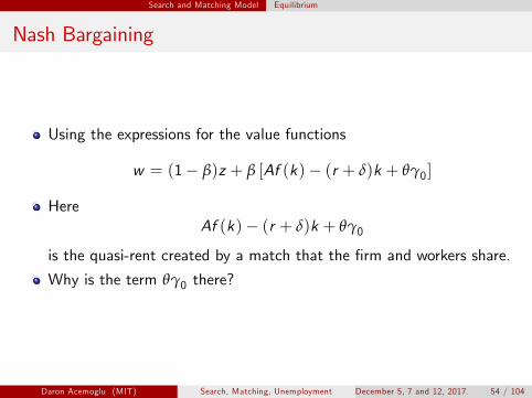
Using the expressions for the value functions

w = (1 − β)z + β [Af (k) − (r + δ)k + θγ0 ]

Here Af (k) − (r + δ)k + θγ0

is the quasi-rent created by a match that the firm and workers share.

Why is the term θγ0 there?



Digression: Irreversible Capital Investments

Much more realistic, but typically not adopted in the literature (why not?)

Suppose k is not perfectly reversible then suppose that the worker captures a fraction β all the output in bargaining.

Then the wage depends on the capital stock of the firm, as in the holdup models discussed before.

w (k) = βAf (k) r + δ

Af 0(k) = ; capital accumulation is distorted 1 − β


Search and Matching Model Steady State

Steady State Equilibrium

1

2

Steady State Equilibrium is given by four equations

The Beveridge curve: s

u = s + θq(θ)

Job creation leads zero profits:

Af (k) − (r + δ)k − w − (r + s)

γ0q(θ) = 0

3 Wage determination:

w = (1 − β)z + β [Af (k) − (r + δ)k + θγ0 ]

4 Modified golden rule: Af 0(k) = r + δ



Steady State Equilibrium (continued)

These four equations define a block recursive system

(4) + r −→ k

k + r + (2) + (3) −→ θ, w

θ + (1) −→ u



Steady State Equilibrium (continued)

Alternatively, combining three of these equations we obtain the zero-profit locus, the VS curve.

Combine this with the Beveridge curve to obtain the equilibrium.

(2), (3), (4) =⇒ the VS curve

r + δ + βθq(θ)(1 − β) [Af (k) − (r + δ)k − z ] − γ0 = 0

q(θ)

Therefore, the equilibrium looks very similar to the intersection of “quasi-labor demand” and “quasi-labor supply”.



Steady State Equilibrium in a Diagram



Comparative Statics of the Steady State

From the figure:

s ↑ U ↑ V ↑ θ ↓ w ↓ r ↑ U ↑ V ↓ θ ↓ w ↓ γ0 ↑ U ↑ V ↓ θ ↓ w ↓ β ↑ U ↑ V ↓ θ ↓ w ↑ z ↑ U ↑ V ↓ θ ↓ w ↑ A ↑ U ↓ V ↑ θ ↑ w ↑

Can we think of any of these factors is explaining the rise in unemployment in Europe during the 1980s, or the lesser rise in unemployment in 1980s in in the United States?



Dynamics

It can be verified that in this basic model there are no dynamics in θ. (Why is that? How could this be generalized?)

But there will still be dynamics nonemployment because job creation is slow.

We will later see how important these dynamics could be.


Effi ciency Effi ciency of Search Equilibrium

Effi ciency?

Is the search equilibrium effi cient?

Clearly, it is ineffi cient relative to a first-best alternative, e.g., a social planner that can avoid the matching frictions.

Instead look at “surplus-maximization” subject to search constraints (why not constrained Pareto optimality?)



Search Externalities

There are two major externalities

θ ↑ =⇒ workers find jobs more easily ,→ thick-market externality =⇒ firms find workers more slowly ,→ congestion externality

Why are these externalities?

Pecuniary or nonpecuniary?

Why should we care about the junior externalities?


Intuition?


Effi ciency of Search Equilibrium

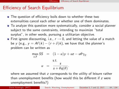
The question of effi ciency boils down to whether these two externalities cancel each other or whether one of them dominates. To analyze this question more systematically, consider a social planner subject to the same constraints, intending to maximize “total surplus”, in other words, pursuing a utilitarian objective. First ignore discounting, i.e., r → 0, and letting the value of a match be y (e.g., y = Af (k) − (r + δ)k), we have that the planner’s problem can be written as

max SS u,θ

= (1 − u)y + uz − uθγ0.

s.t. s

u = . s + θq(θ)

where we assumed that z corresponds to the utility of leisure rather than unemployment benefits (how would this be different if z were unemployment benefits?)



Effi ciency of Search Equilibrium

Why is r = 0 useful?

It turns this from a dynamic into a static optimization problem.

Form the Lagrangian: � � s L = (1 − u)y + uz − uθγ0 + λ u −

s + θq(θ)

The first-order conditions with respect to u and θ are straightforward:

(y − z) + θγ0 = λ

θq0 (θ) + q (θ)uγ0 = λs

(s + θq(θ))2



Effi ciency of Search Equilibrium (continued)

The constraint will clearly binding (why?) Then substitute for u from the Beveridge curve, and obtain:

γ0 (s + θq (θ)) λ =

θq0 (θ) + q (θ)

Now substitute this into the first condition to obtain � � � � θq0 (θ) + q (θ) (y − z)+ θq0 (θ) + q (θ) θγ0 − γ0 (s + θq (θ)) = 0

Simplifying and dividing through by q (θ), we obtain

s + η(θ)θq(θ)[1 − η(θ)] [y − z ] − γ0 = 0.

q(θ)

where ∂M (U ,V )

θq0 (θ) U η (θ) = − = ∂U

q (θ) M (U, V ) is the elasticity of the matching function respect to unemployment.



Comparison to Equilibrium

Recall that in equilibrium (with r = 0) we have

s + βθq(θ)(1 − β)(y − z) − γ0 = 0.

q(θ)

Comparing these two conditions we find that effi ciency obtains if and only if the Hosios condition

β = η(θ)

is satisfied In other words, effi ciency requires the bargaining power of the worker to be equal to the elasticity of the matching function with respect to unemployment. This is only possible if the matching function is constant returns to scale. What happens if not? Intuition?



Effi ciency with Discounting

Exactly the same result holds when we have discounting, i.e., r > 0

In this case, the objective function is Z ∞ SS∗ = e−rt [Ny − zN − γ0 θ(L − N)] dt

0

and will be maximized subject to

N = q(θ)θ(L − N) − sN

Simple optimal control problem.



Effi ciency with Discounting (continued)

Solution:

r + s + η(θ)q(θ)θ y − z − γ0 = 0

q(θ) [1 − η(θ)]

Compared to the equilibrium where

r + s + βq(θ)θ (1 − β)[y − z ] + γ0 = 0

q(θ)



Effi ciency with Discounting

Again, η(θ) = β would decentralize the constrained effi cient allocation.

Does the surplus maximizing allocation to zero unemployment?

Why not?

What is the social value unemployment?


Assignment Models

Assignment Models

An alternative and complement to the search models are the “assignment” models in which heterogeneous workers are assigned to heterogeneous firms but in a frictionless manner. These models were first proposed by Tinbergen (1956) and Koopman and Beckman (1957). We will now review a basic version of assignment models and then show how they can be applied to the analysis of CEO market and generate implications about superstar phenomena. In fact, there turns out to be two related but distinct assignment models:

1 Variable labor assignment models (where each job/task can hire as many units of labor as it wishes, so that there is “many-to-one” matching).

These models also usually feature endogenous prices for jobs/tasks, since otherwise the most productive ones may hire all workers.

2 Fixed labor assignment models (where each job can hire at most one worker, so that there is “one-to-one” matching).


Assignment Models Variable Labor Assignment Model

Variable Labor Assignment Model

Consider an economy based on Sattinger (1979) with a distribution of jobs (firms) of complexity x with distribution G (x), which is taken to be continuous for simplicity and its measure is normalized to 1.

Each job can hire as many units of labor as it wishes.

There is also a set of worker, each supplying one unit of labor inelastically. Each worker has a skill level s, with the distribution H(s), also assumed to be continuous.

All workers have access to an outside wage w , which for now can be normalized to 0.

We will characterize the equilibrium in terms of an assignment function, σ, such that in equilibrium s = σ(x) (or more generally s ∈ σ(x) when we have a correspondence), and a wage function, w (s).



Absolute Advantage

Suppose that a firm of type x and a worker of type s jointly produce revenue

f (x , s)

which is assumed to be twice differentiable and strictly increasing in s, which corresponds to absolute advantage.

We will study competitive equilibria where the labor market for each type of skill clears with a wage w (s).

When a competitive equilibrium exists, it will also be effi cient, so it can be studied as a solution to a planner’s problem as well.

In what follows, we will assume that all types of firms will be active (i.e., the market will not be dominated by just one type of firm etc.).



Proportional Comparative Advantage

We will also assume that f is (proportional) comparative advantage or is weakly log supermodular, i.e.,

fxs (x , s)f (x , s) ≥ fx (x , s)fs (x , s).

We will say that there is strict comparative advantage if this inequality is strict everywhere.

Weak comparative advantage is equivalent to fs (x , s)/f (x , s) being nondecreasing in x , while strict comparative advantage corresponds to this being strictly increasing in x . This in particular implies that the increase in productivity due to greater skills is increasing in the complexity of the job.

We will next see why this is the relevant condition.



Prices

Prices can be introduced straightforwardly into this framework.

First, there might be a given set of prices, p(x), for the goods produced by different types of firms. This can be combined with the f function without any complication.

Second, these prices might be endogenously determined as a function of the level of production (and thus the skill levels of workers assigned to specific jobs).

The approach here does not make assumptions on prices.

But prices might play an important role in ensuring that all types of firms are active.



Understanding Comparative Advantage

The simplest way of understanding why proportional comparative advantage is the right notion here is to consider the unit labor requirement of a job of type x for a worker of skill s.

This is given by 1

l(x , s) = f (x , s)

(this is the labor requirements for producing one unit of output).

Then the unit cost function of firm x depending on the type of labor it hires is

w (s)C (s |x) = w (s)l(x , s) = .

f (x , s)

This cost function, and the fact that firms will operate at the minimum of this cost, is independent of prices, so applies exactly even when prices are endogenous.



Understanding Comparative Advantage (continued)

0Suppose now that we have an assignment s = σ(x) and s = σ(x 0) where s 0 > s and x 0 > x . Then from cost minimization:

w (s) w (s 0) w (s 0) w (s)≤ and ≤ .f (x , s) f (x , s 0) f (x 0 , s 0) f (x 0 , s)

Rearranging these two inequalities, we have

0f (x , s 0) w (s 0) f (x , s 0)≥ ≥ ,f (x 0 , s) w (s) f (x , s)

or in other words, proportionately, production increases more rapidly by hiring a more skilled worker than the wage does at a more complex job and less rapidly at a less complex job.

As s 0 → s, this condition can be satisfied only if f satisfies (weak) comparative advantage.



Positive Assortative Matching

The same argument also establishes why, with strict comparative advantage, σ must be strictly increasing single-value function. In other words, there must be positive assortative matching, whereby higher skilled workers are matched with higher complexity jobs.

0Suppose that we have an assignment s = σ(x 0) and s = σ(x) where s 0 > s and x 0 > x . Then, with the same argument,

0f (x , s) w (s) f (x , s)≥ ≥ ,f (x 0 , s 0) w (s 0) f (x , s 0)

but the outer inequalities violates strict comparative advantage.



Equilibrium Characterization

Now take an increasing σ (with well defined inverse σ−1).

Cost minimization of the firm type x hiring worker type x implies

Cs (s |x) = w 0(s)l(x , s) + w (s)ls (x , s) = 0,

or w 0(s) ls (σ−1(s), s)

= − . w (s) l(σ−1(s), s)



Equilibrium Characterization (continued)

This differential equation can also be written as

d log w (s) ∂ log l(σ−1(s), s) ∂ log f (σ−1 (s), s) = − = .

ds ∂s ∂s

This differential equation, together with an appropriate boundary condition, defines a unique equilibrium wage function.

The boundary condition is given by the requirement that the lowest type firm, x , employing the lowest type worker, s = σ(x), must make zero profits, and thus

w (s) = f (x , s).

In general, it is not possible to make much more progress without specifying some functional forms.



Implications of Comparative Advantage

To understand the wage implications of strict comparative advantage, suppose that there is only weak (and no strict) comparative advantage, i.e.,

fxs (x , s)f (x , s) = fx (x , s)fs (x , s).

(Or more formally, take the limit as we converge from strict to weak comparative advantage). This in particular implies that f is multiplicatively separable:

f (x , s) = f x (x)f s (s).

Then d log w (s) ∂ log f s (s)

= ,ds ∂s

and thus the wage distribution has the same shape as the skill distribution.



Implications of Comparative Advantage (continued)

Conversely, when there is strict comparative advantage, i.e.,

fxs (x , s)f (x , s) > fx (x , s)fs (x , s),

we have that high skill workers earn more than what would be implied by the inequality in skills.

Specifically, for s 0 > s

w (s 0) f (σ(s), s 0)> ,

w (s) f (σ(s), s)

so that high skill workers earn more relative to low skill workers than would be implied by their productivity differences in the fixed job.

Sattinger (1979) also shows that this condition leads to right-skewed wage distributions.



Alternative Model of Proportional Comparative Advantage

Instead of assuming a fixed set of firms with given distribution of job types, the same results also follows if there is one-to-one matching but free entry.

Suppose the production function is again given by f (x , s), satisfying comparative advantage as defined above.

This leads to positive assortative matching, i.e., σ(x) is strictly increasing.



Alternative Model (continued)

A firm can choose to create any job type, so that in equilibrium we must have that, if s = σ(x), then

f (x , s) = w (s) and

0f (x , s 0) ≤ w (s 0), for any s .

Now divide both sides of the inequality by the quality for type s to obtain

f (x , s 0) w (s 0)≤ ,f (x , s) w (s)

so that we end up with the same conditions, and consequently with the same wage function.



Examples

Suppose that f (x , s) = xs, and both variables are uniformly distributed over [ε, 1 + ε], and this immediately implies σ(x) = x .

The wage equation is given as a solution to:

d log w (s) ds

= 1 , s

and thus w (s) = s,

confirming the result that without strict comparative advantage, the wage distribution inherits the properties of the skill distribution.



Examples (continued)

sNow suppose that f (x , s) = ex 1−α α

, and that again both variables are uniformly distributed over [ε, 1 + ε], which once again immediately implies that σ(x) = x .

The wage equation is given as a solution to:

d log w (s) = α,

ds

and thus αsw (s) = e ,

now confirming that with strict comparative advantage, the wage distribution will be skewed to the right with greater inequality in wages than in the skill distribution.


Assignment Models Assignment with One-to-One Matching

One-to-One Matching

Consider next the case of one-to-one matching, again with production function f (x , s). In this situation, if an equilibrium assignment is given by σ, then we must have

0 0f (x , σ(x 0)) − w (σ(x 0)) ≥ f (x , σ(x)) − w (σ(x))

f (x , σ(x)) − w (σ(x)) ≥ f (x , σ(x 0)) − w (σ(x 0))

This immediately suggests that the relevant condition for positive assortative matching in this case will be not log supermodularity, but supermodularity.

In other words, the right notion of comparative advantage will be “level” comparative advantage requiring that

0 0f (x , s 0) + f (x , s) ≥ f (x , s 0) + f (x , s).



Supermodularity vs. Log Supermodularity

Neither supermodularity nor log supermodularity is always stronger.

But when the functions are monotone and both of their arguments, then log supermodularity implies supermodularity.

In particular, note that

∂2 ln f fxs − fx fs = ,

∂x∂s f 2

so if both fx ≥ 0 and fs ≥ 0 are true, ∂2 ln f ≥ 0 implies fxs ≥ 0.∂x ∂s



Equilibrium Characterization

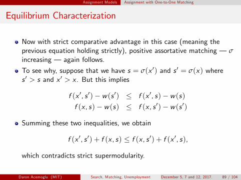
Now with strict comparative advantage in this case (meaning the previous equation holding strictly), positive assortative matching – σ increasing – again follows.

0To see why, suppose that we have s = σ(x 0) and s = σ(x) where s 0 > s and x 0 > x . But this implies

0 0f (x , s 0) − w (s 0) ≤ f (x , s) − w (s)

f (x , s) − w (s) ≤ f (x , s 0) − w (s 0)

Summing these two inequalities, we obtain

0 0f (x , s 0) + f (x , s) ≤ f (x , s 0) + f (x , s),

which contradicts strict supermodularity.



Equilibrium Wages

Now equilibria wages can also be derived in a similar fashion.

Given an assignment function σ(x), the equilibrium must satisfy for any s 0 > s:

f (σ−1(s 0), s 0) − w (s 0) ≥ f (σ−1 (s 0), s) − w (s)

f (σ−1(s)) − w (s) ≥ f (σ−1 (s), s 0) − w (s 0)

0Now take the first inequality and set s = s + ε. As ε → 0, this weak inequality becomes an equality. Dividing both sides of this relationship by ε and taking limits, we have that w insert must also be differentiable and satisfy

dw (s) = fs (σ−1(s), s).ds



Equilibrium Wages (continued)

This differential equation determines the equilibrium wage distribution for a given assignment function σ, and an appropriate boundary condition, now depending on which side of the market is in excess supply. Supposing that workers are in excess supply, for example, this would be

w (s) = w .

Note also that the differential equation for wages can be rewritten in terms of firm characteristics by using a change of variables.

In particular, note that ds = σ0(x)dx ,

so that dw (x)

= fs (x , σ(x))σ0(x).ds


Assignment Models The Market for CEOs

The Market for CEOs

An obvious application of these models is to the market for CEOs, e.g., Tervio (2008). All of the characterization above applies, except that now we should think of x is some characteristic of the firm and s the skill of the candidate manager. Tervio also argued that x should be related to the firm’s market value, so that higher market value (higher size) firms should hire more skilled managers. (Baker, Jensen and Murphy, 1988, Baker and Hall, 2004, as well as Gabaix and Landier, 2006, provide evidence for this). One important implication is that when f exhibits supermodularity, the compensation for managers at the top, even if they are only slightly more skilled than other managers could be very high. Tervio also propose that calibration method to make inferences from this sort of model. This approach also suggests that very high salaries for CEOs might be a result of competitive market forces, not rent-seeking.



Why Supermodularity?

Does supermodularity make sense?

Here is one argument: suppose that a manager of skill s makes a mistake and bankrupts the company with probability e−s , and has no impact on company value otherwise.

Then the expected contribution of the manager is

(1 − e−s ) × non-bankruptcy market value

This would imply a strong form of supermodularity.



The Shape of CEO Pay

A closely related paper by Gabaix and Landier (2006) pushes the assignment model of CEO pay further in three dimensions:

It identifies x with firm size empirically. It proposes a specific shape for the distribution of skill based on

1

2

3

extreme value theory. It confronts the predictions of such a model with data.

The conclusion of Gabaix and Landier (2006) even more strongly than Tervio’s is that the major outlines of the increase in CEO pay can be accounted by competitive market forces.



Extreme Value Theory

Extreme value theory is concerned with the distribution of the maximum of the draws from some distribution G .

A well-known result is that extreme value distributions take the form of one of: Gumbel, Weibull or Frechet.

Gabaix and Landier note that for all “regular” continuous distributions (e.g., uniform, normal, log normal, exponential, and Pareto), the assignment function σ also has a simple form.



Extreme Value Theory (continued)

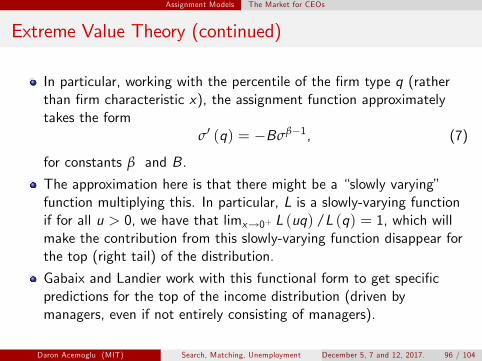
In particular, working with the percentile of the firm type q (rather than firm characteristic x), the assignment function approximately takes the form

σ0 (q) = −Bσβ−1 , (7)

for constants β and B.

The approximation here is that there might be a “slowly varying” function multiplying this. In particular, L is a slowly-varying function if for all u > 0, we have that limx →0+ L (uq) /L (q) = 1, which will make the contribution from this slowly-varying function disappear for the top (right tail) of the distribution.

Gabaix and Landier work with this functional form to get specific predictions for the top of the income distribution (driven by managers, even if not entirely consisting of managers).



CEO Talent and Firm Size

Moreover, Gabaix and Landier posit that the contribution of the CEO to firm value can be written as

¯

Γn(q)γs,

where n(q) is the size of the qth percentile firm.

Then using the differential equation derived above, the equilibrium wage function (for the wage of manager assigned to a firm of the qth percentile) will satisfy

w 0(q) = Γn(q)γσ0(q), or

q), Z q

w (q) = −Γ n(z)γσ0(z)dz + w ( (8) q

where q is the rank of the lowest percentile manager employed.


¯


CEO Talent and Firm Size (continued)

Gabaix and Landier also posit that the firm size distribution is Pareto, i.e.,

n(q) = Aq−α .

This equation with α approximately equal to 1 appears to be a good approximation to the US firm size distribution, for example.

Now combining this with (7) and (8), we have

AγBΓ −(αγ−β)w (q) = q ,αγ − β

where we assume that αγ − β > 0.

Note that as anticipated already, the earning distribution is much more disperse at the top than the skill distribution. For example, if β > 0, there is an upper bound to manager skill. But wages at the very top of are unbounded.




∗Now taking some percentile of the firm size distribution, say q , as the reference size (e.g., the largest 250th firm etc.), noting that

∗ )β−1n(q ∗ ) = A(q ∗ )−α and σ0(q ∗ ) = B(q ,

this can be rewritten as

∗ )β/αw (q) = C (q ∗ )n(q n(q)γ−β/α ,

where C (q ∗) is a constant independent of firm size, given by C (q ∗) = −Γq ∗ σ0(q ∗)/(αγ − β). Or taking logs,

β αγ − βlog w (q) = constant + log n(q ∗ ) + log n(q),

α α

which links log earnings of top CEOs to the average (or reference firm) firm size and own firm size.




More specifically, this equation implies that:

In the cross-section, a 1% increase in firm size leads to a αγ−β percent α increase in CEO pay. In the time series, a 1% increase in the size of all firms leads to a γ percent increase in the pay of CEO employed by a given percentile firm. Across countries, CEOs employed in economies with bigger firms will be pay higher wages, with an elasticity of β/α (presuming that CEO markets are national).

December 5, 7 and 12, 2017. 100 /Daron Acemoglu (MIT) Search, Matching, Unemployment 104

Assignment Models Empirical Evidence

Empirical Evidence

Gabaix and Landier provide a number of correlations consistent with the predictions of this wage equation.

In particular, they show that CEO pay increases with an elasticity of about 0.35 with the firm’s market capitalization and with an elasticity of 0.7 with the market capitalization of the largest 250th firm in the US market.

They also show cross-country correlations consistent with these overall pattern.


(7) (8)Top 500

.33 .23(.043) (.074)(.026) (.057).74 .84(.094) (.080)(.081) (.11)0.023(.016)(.007)YES NONO YES3474 4156

. 9 0.32 0.63

Empirical Evidence: US Panel © Oxford University Press. All rights reserved. This content is excluded from our Creative Commons license. For more information, see https://ocw.mit.edu/help/faq-fair-use/

https://ocw.mit.edu/help/faq-fair-use/


Empirical Evidence: Cross-Country Evidence

© Oxford University Press. All rights reserved. This content is excluded from our Creative Commons license. For more information, see https://ocw.mit.edu/help/faq-fair-use/

Table:

ln(total compensation) (1) (2) (3) (4)

ln(median net income) 0.38 0.41 0.36 0.36 (0.10) (0.098) (0.096) (0.12)

ln(pop) -0.16(0.092)

ln(gdp/capita) 0.12 (0.067)

“Social Norm” -0.018(0.012)

Observations 17 17 17 17 R-squared 0.48 0.57 0.58 0.52


https://ocw.mit.edu/help/faq-fair-use/


Bottom Line

The bottom line is that there are theoretically interesting reasons to think that CEO pay explosion may be due to rent seeking or may be due to market forces.

There are correlations in the data that could be consistent with either.

Probably both of them are going on, and the relative weights are unknown.

So one should probably not jump to strong conclusions, and instead see if there are empirical strategies that could estimate their relative contributions to the CEO pay increase.


MIT OpenCourseWare https://ocw.mit.edu

14.661 Labor Economics I Fall 2017

For information about citing these materials or our Terms of Use, visit: https://ocw.mit.edu/terms.

https://ocw.mit.edu/

https://ocw.mit.edu/terms

labor 14.661. 11-13: matching and unemployment · daron acemoglu (mit) search, matching,...

Documents