IZA DP No. 406

Labor Market Flows and Equilibrium SearchUnemploymentPietro GaribaldiEtienne Wasmer

DI

SC

US

SI

ON

PA

PE

R S

ER

IE

S

Forschungsinstitutzur Zukunft der ArbeitInstitute for the Studyof Labor

November 2001

Labor Market Flows and Equilibrium Search Unemployment

Pietro Garibaldi Bocconi University and CEPR

Etienne Wasmer ECARES, ULB, Université de Metz, CEPR and IZA, Bonn

Discussion Paper No. 406 November 2001

IZA

P.O. Box 7240 D-53072 Bonn

Germany

Tel.: +49-228-3894-0 Fax: +49-228-3894-210

Email: iza@iza.org

This Discussion Paper is issued within the framework of IZA’s research area Mobility and Flexibility of Labor. Any opinions expressed here are those of the author(s) and not those of the institute. Research disseminated by IZA may include views on policy, but the institute itself takes no institutional policy positions. The Institute for the Study of Labor (IZA) in Bonn is a local and virtual international research center and a place of communication between science, politics and business. IZA is an independent, nonprofit limited liability company (Gesellschaft mit beschränkter Haftung) supported by the Deutsche Post AG. The center is associated with the University of Bonn and offers a stimulating research environment through its research networks, research support, and visitors and doctoral programs. IZA engages in (i) original and internationally competitive research in all fields of labor economics, (ii) development of policy concepts, and (iii) dissemination of research results and concepts to the interested public. The current research program deals with (1) mobility and flexibility of labor, (2) internationalization of labor markets, (3) the welfare state and labor markets, (4) labor markets in transition countries, (5) the future of labor, (6) evaluation of labor market policies and projects and (7) general labor economics. IZA Discussion Papers often represent preliminary work and are circulated to encourage discussion. Citation of such a paper should account for its provisional character.

IZA Discussion Paper No. 406 November 2001

ABSTRACT

Labor Market Flows and Equilibrium Search Unemployment∗

This paper explicitly differentiates between unemployment and inactivity, by defining inactivity as a state in which individuals do not search for jobs when non-employed. Facing changes in the value of inactivity, individuals transit through three labor market states. In steady-state, we hence have a theory of equilibrium unemployment determined by both matching frictions and labor market participation margins. The paper firstly rationalizes and quantitatively accounts for the existence of large flows between employment, unemployment and inactivity. Secondly, it shows that unemployment and aggregate wages rise because some of the employed workers are unattached to the labor force, in the sense that they join the inactive pool when they lose a job. Thirdly, unemployment income has little effects on employment, since it attracts people into the labor force and rises the share of attached workers. Finally, our theory suggests that contrary to two-state models, taxation of market activity increases non-participation, unattachment and adversely affects unemployment. JEL Classification: J2, J30 Keywords: Unemployment, matching, home production Etienne Wasmer ECARES Université Libre de Bruxelles CP 114 Avenue Franklin D. Roosevelt 39 1050 Brussels, Belgium Tel.: +32 2 650 4212 Fax: +32 2 650 4475 Email: ewasmer@ulb.ac.be

∗ We thank M. Burda, P. Cahuc, M. Dewatripont, E. Faraglia, C. Wyplosz, G. Violante, F. Panunzi, and particularly C. Michelacci and C. Pissarides, for helpful comments, as well as seminar participants at ECARES-ULB, Bank of Italy (Ente Einaudi), Humboldt Universitätt, Berlin, Lausanne (DEEP-HEC), Geneva (IUHEI) Séminaire Fourgeaud in Paris, CEMFI (CEPR Workshop on Unemployment, Redistribution and Inequality), LSE, and the CEPR European Summer Symposium in Labour Economics (ESSLE). We are also indebted to Robert Shimer who kindly provided us with the gross US flows data.

1 Introduction

In the labor market, individuals face both idiosyncratic and aggregate shocks. This leadsthem to take important labor market participation and employment decisions. In aggre-gate, the transitions resulting from these individual decisions generate extremely large flowsbetween labor market states. Labor force surveys are partly able to recover these flowsby classifying individuals in the working age population across three labor market states:employment, unemployment, and out of the labor force. Table 1 reports the magnitude oflabor market flows across the three labor market states for the US in any given month. Itnotably shows that there are huge flows of individuals between employment and out of thelabor force. Quantitatively, the number of workers who leave the labor market when theylose their job is larger than the number of workers who join the unemployment pool upon jobseparation. In this paper, we will refer to the latter type of workers as the attached work-ers, while the former type of workers are the unattached workers. Our view is that theselarge flows have a lot to tell to both labour and macroeconomists. Indeed, employment andunemployment changes strongly depend on either the exit rate from employment, notablymovements to inactivity, or the entry into unemployment (including movements from inac-tivity). A proper understanding of aggregate labor market flows must therefore necessarilyconsider the distinction between attached and unattached workers (see notably Blanchardand Diamond, 1992, and Burda and Wyplosz, 1994 for similar concerns).1

Table 1: Average Monthly Flows in the US Labor Market. Millions of Workers; February1994-November 2000

EU EN UE UN NU NE15-64 Population 1.88 4.25 2.18 2.08 1.53 3.8124-54 Population 1.16 2.04 1.26 1.02 0.7 1.80E is employment, N is out of the labor force and U is unemployment;

The first (second) letter refers to the source (destination) population

e.g. EU is the employment unemployment flow.

Source: Authors’ calculation on data provided by Robert Shimer.

Beyond labour market flows, there is also a prevalent recognition that understanding thenature and the determinants of the frontier between non-participation and unemploymentcan improve the understanding of the labour market equilibrium stocks. Juhn et al. (1991)and especially Murphy and Topel (1997) argued that the most precise picture of the labormarket is obtained considering jointly non-employment and unemployment figures2. Further,the relative size of the labor market, as indicated by the employment population rates, variessubstantially across OECD countries, and this cross sectional variation is much more linked

1Related to the theme of our work although with a less macroeconomic focus, Abraham and Shimer(2001) argue that changes in unemployment duration in the US. are a consequence of greater labor marketattachment for women. This result as well as the use of three states flow data was obtained earlier for Francein Wasmer (1997).

2Murphy and Topel (1997) argue also that the unemployment rate itself became less and less informa-tive over time, as witnessed by the declining employment rate of young unskilled men, despite a constantunemployment rate.

2

to participation than to unemployment. As the regressions in Table 2 suggest, movementsin participation statistically account for most (93%) of the variance of the employment-population ratio, while unemployment differences statistically account for less than halfof it (49%). In other words, investigating the determination of participation levels acrosscountries is an urgent work to undertake, especially if we want to understand why countriesare characterized by labor markets of very different sizes.

Table 2: Employment Population Rates Across Countries; 1980-1998

Dep. Variable EmploymentPopulationRate

EmploymentPopulationRate

RegressorUnemployment Rate -1.58 -

(0.21) -Participation Rate - 1.08

- (0.08)Num. Observations 21 21R2 0.49 0.93Robust Yes YesStandard errors in parenthesis.

Source: Authors’ calculation on OECD data.

Since both flows and stocks of participants and non-participants are interdependent inseveral obvious ways, it is natural to argue that macroeconomic theories of the labor marketshould not ignore participation and non-participation decisions. The macroeconomic theoryof the labor market that we propose accounts for the statistical classification made in theempirical analysis of the labor market, notably the distinction between unemployment andinactivity and accounts for five of the six possible flows between the three labor marketstates and investigates their determinants. It helps us to understand the links between thestock of unemployment, the employment rate and the participation decisions. More precisely,we explore the impact of participation margins on equilibrium employment, unemployment,aggregate wages, aggregate job creation and aggregate participation and provide new insightson equilibrium unemployment and on the effects of taxation. Finally, our approach help usto understand the respective role of redistribution to inactivity (housing and family benefits)and unemployment benefits.Specifically, we model participation to the labor market in a flows-matching macroe-

conomic model. We start from the convenient Pissarides (1990) and Mortensen-Pissarides(1994) approach, on which we build on. We specify new margins, i.e. arbitrage of workersbetween activity and inactivity. Our three states representation of the labor market adds twonew margins: the quit margin on which workers are indifferent between employment and in-activity; and the entry margin on which workers are indifferent between being unemployedand inactive. This, in turn, creates a distinction between attached and unattached workers:the latter prefer inactivity to unemployment, while the former prefer unemployment to in-activity. For the sake of clarity, and to avoid to enter the debate on the distinction betweenunemployment and out-of-the-labor force, we define unemployment as a state where workersactively look for a job, and non-participation as a state in which it is optimal for workers

3

not to search for a job.3

Several new insights emerge from our three states representation of the labor market. Weshow that equilibrium unemployment depends, for at least four reasons, on turnover alongthe entry and exit margin of labor supply, and on the flows from employment to inactivity.First, in steady-state the latter flows have to be compensated by inflows of new entrantsto the labor market in order to maintain employment, with an endogenous increase in theaggregate amount of frictions. Second, wages are determined by the comparison of marketproductivity and outside options of workers. The latter do not only depend on unemploymentbenefits, but also on a broader concept of “value of inactivity” (leisure, home production,social values), which affects equilibrium unemployment and wage determination in a way thatstandard models cannot capture. Third, proportional taxation on market activities raisesunemployment, by altering the shadow value of market activity relatively to non marketactivity. Fourth, contrary to standard models, we capture Atkinson and Micklewright’s(1991) intuition of a positive role of unemployment benefits, namely making participationto the labor market more attractive.Perhaps surprisingly, most aggregate models of the labor market have ignored the ex-

istence of three separate labor market states, and have instead worked with a two statesrepresentation of the labor market. Real business cycle models carefully distinguish betweenemployment and non-employment, but fail to recognize unemployment as an independentlabor market state (Benhabib et al. 1991). At the other side of the spectrum, aggregatematching models, arguably a useful tool for dealing with labor market issues, carefully modelemployment and unemployment, with a remarkable understanding of determinants of theirstocks and flows. However, most of these models shut down the participation margin, andhave nothing to say on the huge flows between employment and inactivity.There are two streams of related papers: from the microeconomic side, Seater (1977),

Burdett-Mortensen (1978), Burdett (1979), Burdett-Kiefer-Mortensen-Neuman (1984), Swaim-Podgursky (1994) have successfully investigated the relations between search frictions andlabor supply, with a fixed supply of jobs. Our theoretical distinction between inactivityand unemployment, empirically consistent with Flinn and Heckman (1983), is inspired byBurdett and Mortensen (1978). In the macro-search literature, Bowden (1980), Mc Kenna(1987); Pissarides (1990), chap. 6; Sattinger (1995) have introduced a labor demand sideand endogenous participation, in a way that brings few new insights as compared to thestandard (two states) model of matching. Individuals, whose value of non-market time isheterogenous, decide in a static (though intertemporal) way about their participation tothe labor market. It follows that the flows between activity and inactivity are driven bymacroeconomic changes (in productivity, in unemployment) and are thus mainly cyclical orconjunctural flows. In contrast, our theory, building on both macroeconomic factors and

3Table 1 suggested that there are also large direct flows between inactivity and employment. Scholars ofthe labor market argue that these flows are due to a time aggregation bias, and would disappear if we couldobserve individuals continuously. To receive a job offer, one needs to have been active (even marginally) insearch and accordingly to be classified as unemployed, in line with our theoretical definition of unemployment.This is discussed further in our calibration section.

4

individual (household) shocks, is able to account for permanent, structural flows betweenactivity and inactivity, even when macro-conditions are unchanged.The paper is organized as follows: Section 2 introduces concepts and notation and de-

scribes the mechanics of our model. Section 3 develops the first building block of the paper,labor supply, the entry quit margins, and then introduces the second building block, firmsand wage determination. Section 4 solves for the general equilibrium and equilibrium un-employment. Section 5 establishes the stylized facts for the labor market flows consideredhere, proceeds to a cautious calibration of the model to match these flows and then run com-parative statics for various parameters. Section 6 discusses the links between participationand unemployment, and notably the transition from a two states model (full attachment)to a three states model, and uses these insights to explain why taxation of activity may ormay not be neutral in those two cases. Section 7 discusses further some of our simplifyingassumptions. Section 8 details future works.

2 Description of the model

We think of an economy composed by a continuum of risk neutral individuals, whose aggre-gate measure is normalized to one for simplicity. Individuals can be in three different states:employed in the market, unemployed and engaged in job search, and out of the labor force.This immediately raises a question: are unemployment and out of the labor force differentstates? This recurrent issue should in principle be answered by Flinn and Heckman’s (1983)empirical paper, where they show that U (unemployment) and N (inactivity) are actuallyvery distinct states. Here, our definition of unemployment clearly makes a difference betweenthe two states, since by definition unemployment is a state where people actively look fora job. Note that this is consistent with the ILO definition of unemployment in labor forcesurveys.4

Individuals out of the labor force are statistically inactive or non-participants. Though,they derive some utility from leisure and from home production. We assume indeed thatat inactivity, workers are in reality engaged in full-time home production. Since we wantour model to be as general as possible, we choose a specification of the flows of utilityin non-participation which is consistent with both home production and consumption ofleisure; Becker’s (1965) seminal paper indeed showed that consumption of leisure and homeproduction were formally similar actions, combining time and money to maximize utility.Since activities such as children bearing/rearing, strongly affecting participation to the labormarket, can be viewed as home production, we refer hereafter to home production, but ithas to be kept in mind that this can also be interpreted as leisure consumption or moregenerally as the relative utility of non-participation. Existing estimates suggests that thehousehold sector is large, whether measured in terms of inputs or outputs. Data fromthe Michigan Time Use Survey indicate that an average married couple spends 33 percent

4More work about the distinction between the two states has been done by the Bureau of Labor Statis-tics. Sorrentino (1993, 1995) shows that different definitions of unemployment sometimes yield differentunemployment rates, but the ranking of countries is almost always preserved.

5

of its discretionary time working for paid compensation and 28 percent working at home.Studies that attempt to measure the value of household production indicate that the sectoris very large, with estimates in the range of 20-50 percent of measured gross national product(Eisner’s, 1988).Thus, non-participants are assumed to produce a household good with productivity level

θ that is both stochastic and time varying: home productivity is subject to stochastic shocksthat hit individuals with instantaneous probability λ. Upon the realization of a shock,the home productivity level is drawn from a distribution with support over the intervalθmin, θmax and cumulated distribution function F .Individuals are endowed with 1 unit of time, allocated between three competing activities:

home production, time devoted to job search and units of work. For simplicity, we assumethat time devoted to market activities is an indivisible choice, and we force individuals tobe in or out of the labor force. In the former case, however, they can be employed orunemployed, depending on their history. Employed individuals are matched to a firm andproduce a constant productivity flow y, receive a wage w, and are subject to exogenouslydetermined job destruction shocks at rate δ. Further, we assume separability and linearity toensure that, at the margin, home production can be perfectly substituted to the consumptionof market goods or services: cooking vs. restaurant, personal home cleaning vs. cleaningpersonnel, etc... are example of substitutability.Utility of individuals depends on the labor market state, and we let ui(θ) be the indirect

utility function in each of the states i ∈ {w, u, n}, corresponding, respectively to employment,unemployment and out of the labor force. To simplify, we further assume that unemploymentincome is fixed, independent of labor market history and equal to b. Under these set ofassumptions, the utility flows in the three possible states write:

uw(θ) = w(θ) if employed,

uu(θ) = b, if unemployed,

un(θ) = θ, if out of the labor force,

where the expression w(θ) explicitly allows for the possibility that wages depend on θ. Thiswill be explored in next Section, where in addition it is shown that ∂w/∂θ is a constant ofθ.5

While home production is an individual activity, market activity is obtained with a jointprocess combining an individual worker and a single firm. For simplicity, we assume thateach firm is composed of a single job. Firms come to the market by posting vacancies, whoseaggregate measure is indicated with v, while u indicates the aggregate number of unemployedworkers. The matching process brings together individual vacancies and unemployed workers,and is described by an aggregate matching function m(v, u), where m, which records theaggregate number of matches formed in the market, is assumed to be increasing in botharguments, differentiable with negative second derivatives, and with constant returns toscale. Thus, hires only come from the pool of the unemployed, consistent with the previousdiscussion in introduction. The rate at which vacancies are filled is χ = m(v,u)

v= χ(ψ), with

5The indivisibility of labor market participation that is implicit from uu is discussed in Section 7.2.

6

χ0 < 0. ψ is simply the ratio of vacancy to unemployed, often labeled market tightness.Similarly, the rate at which unemployed workers find a job is p(ψ) = ψχ(ψ) with p0 > 0.Thus, there is a one to one correspondence between p and ψ.Our modelling perspective features home productivity shocks that affect individuals

across labor market states. In the aftermath of a home productivity shock, individualsface two endogenous decisions. When an individual is out of the labor force and engagedexclusively in home production, she will have to decide whether, in light of the new homeproductivity level, she is better off into the labor force as an unemployed worker; further,when an individual is employed and matched to a firm, she will have to decide whether sheshould quit her job and spend her time in home production. We will show that both deci-sions are monotonic in the home productivity level θ, satisfy the reservation property, andare thus fully described by two endogenous cut-off levels. In the rest of the paper, we shallindicate with θν the entry margin, or the home productivity level that makes an individualindifferent between being unemployed or being out of the labor force. Similarly, θq shallindicate the home productivity level that makes an individual indifferent between having ajob or producing individually. In equilibrium θq is larger than θν , so that workers with veryhigh home productivity levels will always be out of the labor force, while workers with homeproductivity level below θν will always be in the labor force. In light of the interpretationof θ previously discussed, individuals with high home productivity are also individuals withhigh preference for leisure. Workers with home productivity level between the two cut-offvalues are in the labor force only when they have a job. Thus, our model features two typesof employees: attached and unattached workers. ’Attached workers’ refers to the employ-ees who join the unemployment pool upon realization of the exogenous destruction shock,while ’unattached workers’ refers to the employees that engage their time entirely in homeproduction upon the realization of an adverse shock. Since the share of unattached workersis increasing with the distance between θq and θν , the proportion of unattached worker isendogenously determined. Figure 1 summarizes the properties of the distribution in a singlechart.To determine wages and the job finding probability p, we follow the traditional matching

literature, and we assume that firms post vacancies until full exhaustion of rents. This, inturn, implies that in equilibrium the expected cost of vacancy posting is equal to the valueof the average job. Since only the unemployed workers look for a job, firms do not considerworkers out of the labor force in their vacancy posting decisions. Wages are the outcome ofa bilateral bargaining process, and are set so as to continuously split the surplus from thejob. At each instant, the worker gets a fraction β of the total surplus. Since separationsare jointly efficient, the quit margin θq implies zero surplus at the level of the match, andthus there is agreement over the endogenous separation decision. The equilibrium of themodel is thus described by the three endogenous variables θq, θν and p, or equivalently, by(θq, θν ,ψ) which are consistent with rent sharing and vacancy posting on the part of firms.The next Section starts the formal derivation of the model, while we postpone to Section 7the discussion of conceptual issues linked to our modelling perspective.

7

θ

U n attach edW orkersW na

U n em p lo yedU

O u t L abo rF o rce N

O u tL abo rF o rce N

A ttach edW orkersW a

E n try M arg in θ υU (θ υ)= N (θ υ)

Q u it M arg in θ q

N (θ q)= W na(θ q)

F (θ )

Figure 1: Distribution of Home Productivity Shocks

3 The model

We here introduce the first building block of the paper, i.e. workers’ decisions regarding theirlabor market status by taking as given the aggregate market conditions p(ψ), and the wagerate. Then, we introduce labor demand, the second block of the paper. In the next Section,we derive the existence and uniqueness conditions.

3.1 Intertemporal value functions

At a steady-state, the employed individual has a present discounted value of utilityW whichwrites:

rW (θ) = w(θ) + δ{Max[U(θ), N(θ)]−W (θ)}+ (1)

λθmax

θmin{Max[W (θ0), U(θ0), N(θ0)]−W (θ)}dF (θ0),

where δ is the job destruction rate, U(θ) is the value of unemployment, and N (θ) is the valueof devoting all one’s time to home production: workers, when hit by a home productivityshock (with intensity λ), decide whether or not to quit their job.Hereafter, we shall assume that, for every θ such that W (θ) > N(θ), then W (θ) > U(θ)

(the unemployed workers never reject a job offer at the anticipated equilibrium wage, itselfdetermined later on through bargaining). This corresponds to a restriction on parametersdenoted by R, which ensures that the market is viable and is simply, as it will be shownex-post, y > b. It follows that the value of unemployment writes:

rU(θ) = b+ p[W (θ)− U(θ)] (2)

+ λθmax

θmin{Max [U(θ0), N(θ0)]− U(θ)}dF (θ0),

8

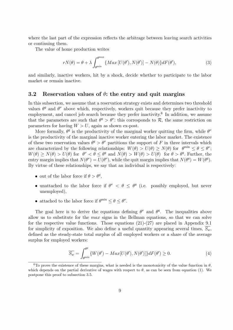
where the last part of the expression reflects the arbitrage between leaving search activitiesor continuing them.The value of home production writes

rN(θ) = θ + λθmax

θmin{Max [U(θ0), N(θ0)]−N(θ)}dF (θ0), (3)

and similarly, inactive workers, hit by a shock, decide whether to participate to the labormarket or remain inactive.

3.2 Reservation values of θ: the entry and quit margins

In this subsection, we assume that a reservation strategy exists and determines two thresholdvalues θq and θν above which, respectively, workers quit because they prefer inactivity toemployment, and cancel job search because they prefer inactivity.6 In addition, we assumethat the parameters are such that θq > θν : this corresponds to R, the same restriction onparameters for having W > U , again as shown ex-post.More formally, θq is the productivity of the marginal worker quitting the firm, while θν

is the productivity of the marginal inactive worker entering the labor market. The existenceof these two reservation values θq > θν partitions the support of F in three intervals whichare characterized by the following relationships: W (θ) > U(θ) ≥ N(θ) for θmin ≤ θ ≤ θν ;W (θ) ≥ N(θ) > U(θ) for θν < θ ≤ θq and N(θ) > W (θ) > U(θ) for θ > θq. Further, theentry margin implies thatN(θν) = U(θν), while the quit margin implies thatN(θq) =W (θq).By virtue of these relationships, we say that an individual is respectively:

• out of the labor force if θ > θq,• unattached to the labor force if θν < θ ≤ θq (i.e. possibly employed, but neverunemployed),

• attached to the labor force if θmin ≤ θ ≤ θν .

The goal here is to derive the equations defining θν and θq. The inequalities aboveallow us to substitute for the max signs in the Bellman equations, so that we can solvefor the respective value functions. Those equations (21)-(27) are placed in Appendix 9.1for simplicity of exposition. We also define a useful quantity appearing several times, Sw,defined as the steady-state total surplus of all employed workers or a share of the averagesurplus for employed workers:

Sw =θq

θmin{W (θ0)−Max[U(θ0), N(θ0)]}dF (θ0) ≥ 0. (4)

6To prove the existence of these margins, what is needed is the monotonicity of the value function in θ,which depends on the partial derivative of wages with respect to θ, as can be seen from equation (1). Wepostpone this proof to subsection 3.5.

9

We can now determine the entry and the quit margins. Replacing the utility flows by theirvalues, using W (θq) = N(θq) one gets the quit margin

λSw = θq − w(θq), (5)

which simply states that for being indifferent between quitting and remaining employed, theutility flows differential between the states must be equal to the forgone value of seeing atransition to a lower θ (which makes the employed worker getting a higher surplus).Noting that W (θν)−U(θν) =W (θν)−N(θν) and with equations (21)-(27), one finds the

entry margin, defined by:

θν − b = p [W (θν)− U(θν)] . (6)

This states that for being indifferent between unemployment and not in the labor force, theutility flows differential between the states must equal the expected gain from searching fora job. Next, we are going to introduce the demand side of the model, by modeling firms’behavior and deriving wages.

3.3 Firms

If the asset value of a vacancy is denoted by VV then the value of a job J(θ) when the workerhas home-productivity θ writes

rJ(θ) = y − w(θ) + (q + δ)(VV − J(θ)) + λθq

θmin[J(θ0)− J(θ)] dF (θ0), (7)

where q = λ(1 − F (θq)) is the quit rate. The right hand side of the equation features thedividend equal to y − w(θ), the operational profits from the job. Further, the firm maylose the worker at rate q, and is left with the value of a vacancy VV . Conversely, with thecomplementary probability (conditional on a change in θ), the firm faces a worker with anew θ, but there is no job separation. Finally the match is also subject to destruction shockat rate δ.Two remarks are in order. First, from the firm’s perspective, the quit rate of all workers

is the same, given the Poisson process assumption. In that, our model is a macroeconomicmodel where firms cannot infer from agents types their separation probability. Second, forsome workers (but not all) w will depend on θ even though θ does not affect the productionof the firm. This arises here because wage bargaining involves the outside option of a worker,which is Max[U(θ), N(θ)].

3.4 Job creation margin

Denoting by c the flow search cost for firms, the value of a vacancy is

rVV = −c+ χ(ψ)[Je − VV ], (8)

10

where

Je =

θν

θminJ(θ0)dF (θ0)F (θν)

,

is the expected value of a match for the firm, conditional on the fact that the worker isactually looking for a job, i.e. has a θ below θν . Indeed, the attached workers are the onlyone looking for a job.The third margin is the job creation margin, stating that firms will enter the market up

to a point at which all market opportunities are exhausted: free entry in the job marketimplies full exhaustion of rents. Thus, substituting VV = 0 in equation (8), the job creationmargin is the solution to

c/χ(ψ) = Je, (9)

which states that the expected search costs are equal to the expected value of a job for thefirm.

3.5 Wage bargaining

To complete the determination of the model we need to specify a wage rule, which weassume to be the standard division of the surplus. In what follows, we denote by S(θ)the total surplus associated with a specific match firm/worker, where the worker has home-productivity θ. Formally, S(θ) reads S(θ) = J(θ)+W (θ)−Max[N(θ), U(θ)]. By substitutingfor the relevant value functions in the definition of the surplus S(θ), one immediately noticesthat the surplus of the unattached workers (for θ ∈ [θν , θq]) depends on the specific valueof θ. However, this is not the case for the attached workers (for θ ∈ θmin, θν ), since theiroutside income is simply b, independently of the specific value of θ. This important property(due to the assumption that unemployed workers do not contribute to home-production, seeSection 7.2 for a discussion) greatly simplifies the analysis, and allows to obtain the followingresults for the attached workers (θ < θν):

• their wage is independent of θ,• their value functions W and U do not depend on θ,

• the expected surplus of a firm that recruits a worker (necessarily an attached one) isindependent of θ.

The surplus S(θ) is shared according to a generalized Nash-bargaining with shares β tothe worker, and 1− β to the firm. The wage rule satisfies

W (θ)−Max(U(θ), N(θ)) = βS(θ). (10)

11

We thus will have two profiles for wages, one for the attached workers, one for the unattachedworkers. Moreover, the two wages read (see Appendix 9.3):

wA = (1− β)b+ β (y + ψc) ∀θ ≤ θν , (11)

wNA(θ) = (1− β)θ + βy ∀θ ≥ θν. (12)

Four important remarks are in order. First, wages of the unattached workers do not dependon the job finding probability. Second, unattached wages are larger than attached wages.This is easy to establish in remarking that

wNA(θ)− wA = (θ − θν)(1− β)

(see Appendix 9.3). This arises from the fact that workers have the same market productivitybut the unattached workers have a better outside option.7 Note that it immediately followsthat wages at the entry margin are continuous, wNA(θ

ν) = wA. Third, our model is consistentwith an upward sloping wage tenure profile, since the worker starts the relationship as anattached worker, and, on average, finishes his or her relationship as an unattached worker.And forth, given J(θq) = 0, one has that w(θq) = y + 1−β

βλSw: the wage of the marginal

worker is above the marginal product, which is a case of labor hoarding. Firms wish to retainthe worker with the hope that she will become a (more) attached worker in the future.Finally, using the wage equations, one can now very easily show that the value functions

W,U and N are either constant or monotonic in θ, and thus that the reservation propertiesin θ assumed in the beginning of 3.2 are valid.

4 General equilibrium

4.1 Definition

Denote by u the unemployment rate, i.e. the ratio of the number of unemployed to the activeworkers; and by n the non-participation rate, i.e. the ratio of the number of inactive workersto the total population (normalized to 1). Given that there is a one-to-one correspondencebetween p and ψ, then:Definition: A market equilibrium is a n-uple (θν , θq,ψ, u, ni) and two wage rules (one

for the attached, one for the unattached workers) satisfying:

• the entry margin for workers,7This may however be difficult to reconcile with existing empirical evidence if unattached workers rep-

resent women and youngsters, individual who enjoy lower wages in the labor market. However, if marketsare segmented, workers with higher transition rates to inactivity, even though they have the same marketproductivity as other workers, will face a lows labor market tighness. This will reduce the average wage ofthe group with high unattachment in general equilibrium. Further, in reality, there may be some negativecorrelation between home and market productivity. Note also all wage differentials across workers in thesame segment of the labour market disappear in Section 7.1 when we model asymmetric information on thevalues of θs.

12

• the quit margin for workers,• the job creation margin for firms,• the steady-state condition for unemployment flows,• the steady-state condition for inactivity flows.

This Section aims at showing the existence (and uniqueness) of such an equilibrium. Thederivation of the general equilibrium can be decomposed in two parts. The first part involvesthree equations solving for three endogenous margins: θq, θν ,ψ. The next part solves for thesteady-state values of the flows given the stocks. The three equations of the first part arethe following:

c

χ(ψ)=(1− β)(θq − θν)r + λ+ δ

, (JC)

θν − b = βcψ

1− β , (Entry)

θq − y = λ

r + λ+ δ

θq

θνF (z)dz. (Quit)

The first one, equation (JC), is obtained after an integration by part from the free-entrycondition on the parts of firms using c

χ(ψ)= JA = J(θν), by continuity. It simply says that

the surplus from a job is equal to the expected search costs. To obtain the second equation,one usesW−U = β/(1−β)J and equation (9) in equation (6). One obtains the intermediateequation

θν − b = p(ψ)β(θq − θν)

r + λ+ δ, (13)

which states that the expected gain of a job is equal to the forgone value of home production.Then, substituting from (JC) into (13) one finally gets a simpler version for the entry margin,equation (Entry). This equation shows that the entry margin θν is increasing (in partialequilibrium) in b, ψ and β, the workers’ share of the surplus. Finally, recalling the quitmargin in equation (5), we obtain the third equation of the model, equation (Quit).Since (Entry) is a linear relation between θν and ψ, one can easily replace θν into equation

(JC) and equation (Quit). Doing so, one obtains two relations between ψ and θq that haveopposite slopes. One thus can express the equilibrium in the space [ψ, θq]. In what followsand notably in Figure 2, we label the modified first equation the job creation curve, andit is positively sloped. The modified third equation is downward sloping, and is labelledquit margin. Proofs of the slopes are placed in the Appendix 9.4. The intercept of theJC curve is b and the intercept of the quit margin curve, denoted by l is defined by l =y + λ

r+λ+δ

l

bdF (θ) > y. Thus, a sufficient condition for existence and uniqueness is y > b.

13

Quit Margin

θq

Job Creation

ψ

Figure 2: General Equilibrium

EmployedAttached

θ<θν

EmployedUnattached

θν<θ<θq

Inactiveθν<θ

Unemployedθ<θν

eaena

enaea

un

uea=p ean=q

eau=δ enan=q+δ

nu

Figure 3: Endogenous Flows between the Different States (Attached Employment;Unattached Employment; Unemployment; Inactivity)

14

4.2 Steady-state unemployment

In this subsection, we calculate the equilibrium stock of workers in different states. Notefirst that employed workers facing a shock δ enter inactivity only if θ > θν and search fora new job if θ ≤ θν . All the flows in the model are represented in Figure 3. Note that alltransition rates are endogenous, except eau = δ which is exogenous, but affects a number ofworkers that is endogenous. With the steady-state assumption, one obtains (the proof is inAppendix 9.5)

u∗ =δ + q

p+ δ + q(14)

with q = λ[1 − F (θq)]. The steady-state stocks of the other states are too complicated forbeing reported here, but can be calculated (see a sketch of the calculation in Appendix 9.5).Equilibrium unemployment deserves four remarks. First, there is a whole new set of

parameters determining equilibrium unemployment, through q, which are linked to inactivityand household shocks. Those parameters are absent from the classical two states analysis ofthe labor market. Second, the effect of the quit rate is in steady-state exactly the same asan increase in the job destruction rate: it increases the inflows into unemployment, becausethe number of people leaving a job for inactivity will be matched by an equivalent number ofworkers entering activity through unemployment. Thus, the transitions from and to inactivityraise the frictional nature of unemployment. Third, as we have seen in the previous Section,there is also an indirect effect of en: the quit rate is anticipated by firms along the jobcreation margin, through a reduction in vacancy posting. There is thus an adverse effect onp and thus on unemployment. Finally, there is also the wage effect of unattachment, whichreduces further job creation of the labor market (and thus raises u∗).

5 Calibration and applications

5.1 The stylized facts

Let us first start with a description of the facts we want to illustrate here. We base ourcalibration on the US flows reported in the introduction. Following Abraham and Shimer(2001), we use the gross monthly flows of workers between the three states E, U and N,applying the Abowd and Zellner (1985) correction for misreported labor market status. Inassuming that the errors have not increased over time and as in Abraham and Shimer, thatthey are in the 1990’s independent of gender, we apply the correction displayed in Abowdand Zellner (pp. Table 5, Classification and Margin Error to Unadjusted). We only considerthe post-February 1994 period (after the CPS survey redesign) for two groups of workers:the 15-64 population (hereafter referred to as ‘total’) and the 25-54 population (‘prime-age’).When the flows are deflated by the origin population, they are called transition rates. Whenthey are deflated by the total (or prime-age) population, they are called ‘flow rates’. Wedeseasonalized these flows using the X12 Census program available in EViews and computedan average for the period 1994:2 to 2000:11. Tables 3 and 4 indicate the sample averages forthe different flows and stocks.

15

Table 3: Average Monthly Flows in the US Labor Market. 15-64 Population

TOTAL eu en ue un nu neTransitions 1.550 3.459 34.37 32.86 4.055 10.11Flow Rates 1.140 2.549 1.306 1.255 0.916 2.228Stocks E/P U/P N/P U/L

73.60 3.835 22.56 4.495E is employment, N is out of the labor force and U is unemployment;

The first (second) letter refer to the source (destination) population

e.g. eu is the employment unemployment flow.

Averages 1994:2 2000:11. Abowd Zellner correction, seasonally adjusted by X11.

Source: Gross CPS data provided by Robert Shimer and Authors’ calculation.

Table 4: Average Monthly Flows in the US Labor Market. 25-54 Population

PRIME AGE eu en ue un nu neTransitions 1.271 2.223 34.33 27.84 3.908 10.06Flow Rates 1.029 1.800 1.105 0.901 0.618 1.586Stocks E/P U/P N/P U/L

80.97 3.253 15.77 3.865E is employment, N is out of the labor force and U is unemployment;

The first (second) letter refer to the source (destination) population

e.g. eu is the employment unemployment flow.

Averages 1994:2 2000:11. Abowd Zellner correction, seasonally adjusted by X11.

Source: Gross CPS data provided by Robert Shimer and Authors’ calculation.

It is remarkable to observe that, even when taking out the extreme of the age distribution,as we do in considering the sample 25-54, one still have large flows from and to inactivity. Itis notably the case that exits from employment to unemployment are less frequent than exitsfrom employment to inactivity. All other flows have conventional values. In that period ofhigh tension of the US labor market, the exit rates from unemployment is very high, above30%. Finally, there are also important direct flows from inactivity to employment, perhapsdue to non-corrected misclassification. To make these flows coherent with our theoreticalspecification, we argue that any person having a job had to make a minimal effort (goingto an interview or negotiating the wage or working conditions). In that sense, this personshould be classified as job seeker at least five minutes, which obviously surveys cannot detect.This well known phenomenon is a time aggregation bias. Indeed, the existence of ne flowsin the CPS survey (as in all other labor force surveys) is a misclassification with respect toour theoretical model, and ne flows should instead add-up to both nu and ue flows.

5.2 Calibration

We calibrate the model on the basis of the flow rate, knowing that the stocks are determinedin steady-state from these flows. As it is obvious from Tables 3 and 4, there are six flows toconsider, while our model can account only for five of them. So, consistent with the modeland the discussion above on the infra-month transitions, our calibration will be based on themodified rates: nu = nu +ne and ue = ue+ ne.Table 5 reports the calibration exercise for the 15-64 population. The spirit of the calibra-

16

tion exercise was to choose parameter values so as to obtain a model economy that resembledthe US labor market in the second half of the nineties. Namely, we calibrated our modeleconomy to have an unemployment rate of 4.5 percent, a participation rate of 76 percent,and a market tightness of 1, which is a reference value for most of the matching literature.Further, we also calibrated the eu flow rate, which Table 5 shows to be 1.14 percent. Inparticular, we search the parameter space for values of y, b, δ, c, x0

8, with the aim of gettingas close as possible to the unemployment rate, the participation rate, market tightness andthe eu flow. This calibration exercise leaves us with the following free parameters: β, η,r, λ as well as the distribution of productivity shocks. We set the pure monthly discountrates r to 0.005, β and η so that they satisfy the Hosios with a standard reference value ofβ = η = 0.5. The distribution of home productivity was exponential (f(θ) = Be−Bθ) withparameter B = 1, while the arrival rate of the idiosyncratic shock λ was exogenously set to0.14.The results of the calibration exercise are reported in the lower part of Table 5. Household

production is approximately one fourth of market production (GNP ), a statistic whichappears to be in line with existing estimates on the size of the informal sector. Table 5shows that the model economy we constructed not only mimics the calibration statistics,but it seems also capable of matching the relative ranking of all the labor market flows,even though the actual degree of resemblance of the various statistics varies across flows. Inparticular, our model economy displays larger en and ue flows than those experienced by theUS economy, and lower un and nu flows. We believe that the main difference between ourstatistics and the US statistics are likely due to two specific assumptions of our model: theabsence of the discouraged worker effect and the homogeneity of labor force types. In reality,it is well documented that unemployment is a state dependent phenomenon, and workersexperiencing long spell of unemployment end up out of the labor force. Accounting for thesephenomena would certainly reduce the model generated ue flow, and would simultaneouslyimprove the match of the un flow. The too large en flow calibrated by our model suggeststhat in reality the share of unattached worker is probably less than the estimated one. Afurther way to improve the calibration exercise would be to solve the model with two typesof workers: one type always attached to the labor force and another type that behaves ina way consistent with the proposed model. Even though these extensions are technicallydoable, we believe that our model is a very good pass for rationalizing the large US labormarket flows.

17

Table 5: Calibration to the US Labor MarketParameters Notation Value US EconomyMatching Elasticity η 0.50Matching Function Constant xo 1.05Unemployed Income b 1.29Discount Rate r 0.005Idiosyncratic Shock Rate λ 0.14Separation Rate δ 0.02Workers’ Surplus Share β 0.50Productivity y 2.61

Minimum Home Production a θmin 0.50Search Costs c 1.18Equilibrium Values

Entry Margin θν 2.47F (θν) 0.71

Quit Margin θq 2.84F (θq) 0.76

Market Tightness φ 1.00Calibrated Statistics

Unemployment Rate u 4.60 4.49Non Participation Rate n 26.00 26.40eu flow rate eu 1.14 1.14Implied statistics

share household gdp 0.26 0.33en flow rate en 2.44 2.54ue flow rate ue 4.84 3.5=1. 3+2.2un flow rate un 0.19 1.2nu flow rate nu 1.06 3.2=0.9+2.2Attached Employed Ea 67.55Non-Attached Employed Ena 3.05Average Wage attached Worker wA 2.54Average Wage non-attached Worker wNA 2.72(a), Distribution is Exponential with parameter B =0.50

Source: Authors’ calculation

5.3 Comparative statics for the 15-64 population

We are now in a position to study the comparative static properties of the model, with thehelp of the simple system of equations (Entry) (JC), and (Quit), the equilibrium unemploy-ment relationship of equation (14), and the calibration exercise solved in Table 5. Let usfirst consider the effect of an increase in y, the aggregate productivity. While the formalderivation is left to Appendix 9.6, we may derive the main intuition with the help of Figure2. The increase in y shifts the quit margin to the right along the job creation curve andinduces an increase in ψ and θq, since the job creation curve does not shift. This impliesan increase in job creation, and a reduction in job destruction, as would be the case in anyreasonable model of the labor market. Further, participation to the labor market goes up,as witnessed by the unambiguous increase in the entry margin in equation (Entry).The general equilibrium effect of b, the specific income of the unemployed is more inter-

esting. In our theoretical perspective, an increase in b is different from the standard effectsin equilibrium models (e.g. Mortensen Pissarides 1999), whereby changes in b simply work

8The total number of contacts is x0ψ−ηV (i.e. x0 is a scale parameter; then η is the elasticity of χ(ψ),

the finding rate of workers by firms.

18

Table 6: Changes in Aggregate Productivity

y ψ θν θq u n Ea E EnaE

wA wNA2.61 1.00 2.47 2.84 4.60 26.00 67.55 70.60 4.32 2.54 2.722.66 1.04 2.52 2.89 4.43 25.27 68.35 71.42 4.29 2.59 2.772.71 1.08 2.57 2.95 4.27 24.57 69.14 72.21 4.26 2.64 2.832.76 1.13 2.62 3.01 4.12 23.88 69.90 72.98 4.23 2.69 2.882.81 1.17 2.67 3.06 3.98 23.21 70.64 73.73 4.19 2.74 2.93u is the unemployment rate; n is the non participation rate

Ea, Ena, and E are respectively attached, non-attached, and total employment.

wa and wna are the average wage of attached and non-attached workers

Source: Authors’ calculation

Table 7: Changes in Unemployed Income

b ψ θν θq u n Ea E EnaE

wA wNA1.29 1.00 2.47 2.84 4.60 26.00 67.55 70.60 4.32 2.54 2.721.45 0.87 2.48 2.82 4.94 26.09 67.43 70.27 4.04 2.54 2.711.61 0.74 2.49 2.80 5.35 26.18 67.26 69.87 3.73 2.55 2.711.77 0.62 2.50 2.79 5.88 26.28 67.03 69.39 3.41 2.55 2.701.93 0.49 2.51 2.77 6.59 26.39 66.67 68.76 3.04 2.56 2.69u is the unemployment rate; n is the non participation rate

Ea, Ena, and E are respectively attached, non-attached, and total employment.

wA and wNA are the average wage of attached and non-attached workers

Source: Authors’ calculation

like a reduction in y, implying a lower job finding rate, ψχ(ψ), and an increase in equilibriumunemployment. The comparative static results show that the increase in b reduces the jobfinding probability, raises the entry margin θυ, and reduces the quit margin θq. In terms ofFigure 2, this corresponds to a shift of job creation to the right, with a simultaneous shift tothe left of the quit margin. The economics of this effect is as follows. Higher b has a directimpact on wages, and reduces job creation and vacancy posting.The effect on θυ is a priori ambiguous: it is the sum of a positive direct effect (through

Entry) and a negative general equilibrium effect working through a lower ψ already discussed.The analytical results however show that θυ unambiguously rises in response to b. Further,b has a negative effect on θq, as shown in Appendix 9.6. Table 7 simulates the comparativestatic effects of b in the general model, using the calibrated economy in Table 5. Thequantitative example suggests that increasing b by as much as 50 percent causes a substantialnegative impact on ψ, a small positive impact on θν and a small negative effect on θq. Sincethere is a decrease in job creation (ψ falls) and an increase in job destruction (θq falls),equilibrium unemployment rises. Further, Table 7 shows that b has a very small effect ontotal employment, since its main effect is to change the composition of employment withmore attached and fewer unattached workers as b rises.

6 Labor market participation and unemployment

Our model has three margins, whereas the search-matching literature usually deals with twomargins, the job creation and the job destruction margins. We are more accurate regardingthe description of the labor supply side of the economy. The first margin, the entry margin

19

(Entry), is a decision of workers only, who decide to look for a job or enjoy home productivity.It is thus a pure labor supply margin. The second one, the quit margin (Quit), is a jointdecision of the pair worker-firm: when the surplus of the match goes to zero, the decisionto destroy the match is jointly efficient. In that sense, the quit margin is not a pure laborsupply margin, but rather a mix of labor supply and labor demand. This is a direct result ofthe wage rule that shares the surplus in fixed proportion β and 1−β. If we were to solve themodel with fixed wages, the quit margin would no longer be a jointly efficient decision, asthe firm would no longer be able to retain a worker willing to quit.9 Finally, the job creationmargin (JC) is a decision of the firm only, and thus belongs to the labor demand side.In what follows, we discuss the first two margins considering what happens when labor

market frictions disappear, and we show that our model converges to a simple frictionlesshome productivity model, traditionally solved in the real business cycle literature. Next, wediscuss a special case of the model, a situation in which the distribution of θ has two masspoints, and we formally show how the equilibrium of the model, notably unemployment andparticipation, depends on the distribution and frequency of home productivity shocks.Thirdly, we show how in such a stylized world, taxation of market activities, neutral

in absence of unattachment, may adversely affect the market economy, by endogenouslyinducing unattachment in equilibrium. Finally, we discuss the dual problem of subsidies toinactivity.

6.1 Properties of labor supply margins

In general equilibrium, an increase of the scale parameter x0 of the matching function toinfinity in equation (13) leads to the convergence of θq and θν to a common limit. Further,using (Quit), one can see that the limit of these two cutoff values is simply y, the value of themarket productivity. The intuition for this limit result is simple: when frictions disappear,the individual who is indifferent between market and non market activities must get a marketreward which is as good as her private return. Indeed, by virtue of wage bargaining, thewage of a market with infinite exit rate from unemployment is simply the flows of profit,and workers receive their marginal product. This implies that w = y = θq. When x0rises indefinitely, individuals can be inactive or employed, but never unemployed, since theinstantaneous probability of finding a job converges to 1. In this latter case, the commonlimit y splits the distribution F into individuals that are employed and non employed.An increase in x0 reduces the quit margin, since the joint value of a job is now lower.

However, larger x0 makes participation to the labor market more attractive, since the prob-ability of finding a job increases. At infinity, the two margins converge to y. An interestingfeature of our economy is that the share of unattached workers in the population, whichwrites F (θq)− F (θν), converges to zero as x0 rises indefinitely. These mechanisms are illus-trated in Figure 5 in the Appendix, which reports the general equilibrium values of (θν , θq)against x0.

9In which case the quit margin would become a pure labor supply margin as the entry margin. SeeSection 7.1 for an application of this concept in the context of asymmetric information.

20

6.2 The transition from full-attachment to unattachment in a spe-cial case

The derivation of general equilibrium highlighted the relation between equilibrium unem-ployment and a new set of parameters, linked to the frequency and the distribution of homeproductivity shocks. In this and the following subsections we explicit the dependence ofequilibrium unemployment to such parameters. To study these relationships in the simplestpossible model, let us assume that the distribution of θ’s is degenerate and has two masspoints θL < θH , and let us denote with αL and αH the shares of the population in eachgroup (obviously αL + αH = 1). The next subsection will show that a proportional taxa-tion to market activity, neutral in standard models of the labor market, adversely affectsunemployment when unattachment exists in equilibrium.In the particular case considered here, the margins θν and θq are still well defined, and

what matters in this example is how they are situated with respect to the mass points θLand θH . The most interesting case is the one in which the high home-productivity level islarger than the unemployed income, but lower than market productivity. In what follows,we assume that θL < b < θH < y, and study two different equilibrium configurations. Werefer to the full-attachment equilibrium (case A) when θL < θH < θ

ν, or simply whenall individuals in the working age population are in the labor force. Further, we will studythe unattachment equilibrium (case B), where θL < θ

ν < θH < θq, a situation in which

individuals in θH are in the labor force only when they have a job. One obtains (Appendix9.8) a single equation determining market tightness ψ which can be written as

r + δ

1− βc

χ(ψ)+

cβ

(1− β)ψ 1− iBαH λ

r + λ+ δ= y − b− iBαH(θH − b) λ

r + λ+ δ, (15)

where iB is an indicator variable equal to zero in the full-attachment equilibrium (A) and 1in the unattachment equilibrium (B).One can immediately stress that in the attached equilibrium, ψ does not depend on λ,

nor on the distribution parameters θH and αH as in a standard macro matching model withfixed labor force participation. Conversely, in the unattached equilibrium all the parameterslinked to the home productivity shocks enter the determination of unemployment. It isnotably easy to derive (in Appendix 9.8 again) that in the unattachment equilibrium, thefollowing general equilibrium results hold

dψ

dλ< 0;

dψ

dθH< 0;

dψ

dαH< 0; if iB = 1. (16)

Equilibrium unemployment rises with the arrival rate of household shocks, with the levelof home productivity θH and with the proportion of individuals in the high productivitystate. This shows the interaction between market unemployment, labor demand and nonmarket parameters. Higher λ implies that a newly hired individual, who is attached bydefinition, is more likely to become unattached, with adverse effects on the expected wagecosts. This, in turn, reduces labor demand and vacancy posting. Equilibrium unemployment(in the unattached equilibrium it is simply u = δ

δ+p(ψ)) rises when ψ decreases. Other results

concerning participation are derived and discussed in Appendix.

21

6.3 Taxation on activity and job creation

Empirical studies on the cross country determinants of unemployment (e.g. Nickell andLayard, 1999) find a negative relationship between taxation and both unemployment andlabor input. In their cross-country reduced form regressions that control for a large setof institutional measures, Nickell and Layard find that the overall tax burden has a clearnegative impact on unemployment and on the employment population ratios. They estimatethat a reduction in the total tax rate of 5 percentage points would reduce unemployment by13 percent (e.g. from 8 percent to 7 percent). Similarly, they find adverse effects of taxationon an index of total labor supply, which takes into account differences in the number of hoursworked in a given year. More substantial unemployment effects were found by other similarstudies, including Daveri and Tabellini (2000) and Scarpetta (1996). Thus, when they reviewthe existing evidence, Nickell and Layard conclude that the balance of the evidence suggeststhat there is some overall adverse effect of taxation on unemployment and labor input.Nevertheless, there is some skepticism over this relationship. Several authors believe that

the correlation between taxation and unemployment is spurious, since it is difficult to find anegative long run effect of taxation on labor costs. The latter point can be illustrated bothempirically and theoretically. First, labor market theories predict that taxation should haveno employment effects as long as its effects is entirely borne on wages, with no impact on totallabor costs (Pissarides, 1998). Second, several papers estimated country-specific time seriesregressions on aggregate labor costs, and found that wages tend to adjust, in the very long-run, to changes in taxation. In other words, despite its empirical relevance, the literaturehas failed to outline a sound transmission mechanism linking taxation to unemployment.We can rationalize the empirical literature in the context of our model. Although we can

do it through simulations in the general case, we can easily illustrate this using the distinctionbetween the two types of equilibria considered above. In what follows, we consider theeffect on unemployment stemming from a proportional increase of taxes levied on all marketactivities. Almost by definition, the non-market activities cannot be taxed instead.Working with the same discrete distribution specified in the previous subsection, let us

assume that market productivity, unemployed income and firms’ vacancy costs are all taxedat rate τ . In other words, in a world with proportional taxation we will have y0 = (1− τ)y,c0 = (1 − τ)c and b0 = (1 − τ)b.10 Substituting these values into equation (15), we stillhave our two different equilibria, depending on the value of the indicator function iB. Letus consider the effect of taxation on the attached equilibrium. In the attached equilibriuman increase in proportional taxation τ has no effect on market tightness, and no effect onequilibrium unemployment. This is not surprising, since such neutrality is a standard resultsof two states constant returns to scale models. As long as taxes are levied proportionallyon all market activities, including unemployment income, there is no relationship betweentaxes and unemployment. Gross wages are also unchanged.Nevertheless, as τ grows out of zero into positive and increasing values, the shadow value

10The fact that wages are not taxed directly is for simplicity, since taxing wages impacts the effective shareof workers who are less demanding. In our specification, i.e. taxing b and y, it is easy to see that the netequilibrium wage of the attached workers is then also proportional to (1− τ).

22

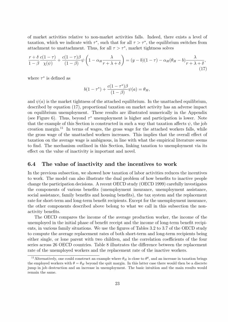
of market activities relative to non-market activities falls. Indeed, there exists a level oftaxation, which we indicate with τ ∗, such that for all τ > τ ∗, the equilibrium switches fromattachment to unattachment. Thus, for all τ > τ ∗, market tightness solves

r + δ

1− βc(1− τ)χ(ψ)

+c(1− τ)β(1− β) ψ 1− αH λ

r + λ+ δ= (y − b)(1− τ)− αH(θH − b) λ

r + λ+ δ,

(17)

where τ ∗ is defined as

b(1− τ ∗) + c(1− τ∗)β

(1− β) ψ(a) = θH ,

and ψ(a) is the market tightness of the attached equilibrium. In the unattached equilibrium,described by equation (17), proportional taxation on market activity has an adverse impacton equilibrium unemployment. These results are illustrated numerically in the Appendix(see Figure 6). Thus, beyond τ ∗ unemployment is higher and participation is lower. Notethat the example of this Section is constructed in such a way that taxation affects ψ, the jobcreation margin.11 In terms of wages, the gross wage for the attached workers falls, whilethe gross wage of the unattached workers increases. This implies that the overall effect oftaxation on the average wage is ambiguous, in line with what the empirical literature seemsto find. The mechanism outlined in this Section, linking taxation to unemployment via itseffect on the value of inactivity is important and novel.

6.4 The value of inactivity and the incentives to work

In the previous subsection, we showed how taxation of labor activities reduces the incentivesto work. The model can also illustrate the dual problem of how benefits to inactive peoplechange the participation decisions. A recent OECD study (OECD 1999) carefully investigatesthe components of various benefits (unemployment insurance, unemployment assistance,social assistance, family benefits and housing benefits), the tax system and the replacementrate for short-term and long-term benefit recipients. Except for the unemployment insurance,the other components described above belong to what we call in this subsection the non-activity benefits.The OECD compares the income of the average production worker, the income of the

unemployed in the initial phase of benefit receipt and the income of long-term benefit recipi-ents, in various family situations. We use the figures of Tables 3.2 to 3.7 of the OECD studyto compute the average replacement rates of both short-term and long-term recipients beingeither single, or lone parent with two children, and the correlation coefficients of the fourseries across 26 OECD countries. Table 8 illustrates the difference between the replacementrate of the unemployed workers and the replacement rate of the inactive workers.

11Alternatively, one could construct an example where θH is close to θq, and an increase in taxation brings

the employed workers with θ = θH beyond the quit margin. In this latter case there would then be a discretejump in job destruction and an increase in unemployment. The basic intuition and the main results wouldremain the same.

23

Table 8: Average Replacement Ratios for Short Term and Long Term Benefit Recipients.

Mean SDa (I)b (II) (III) (IV )(I) ST, single 0.59 0.14 1 0.17 0.79 0.21(II) LT, single 0.38 0.18 1 0.46 0.72(III) ST, lone with two children 0.69 0.13 1 0.59(IV ) LT, lone with two children 0.57 0.16 1Number of Countries: 26

ST is short term; LT is long terma standard deviationb correlation coefficients

Source: OECD 1999 and Authors’ calculation.

As expected, the short-term replacement rates are in average higher than the long-termreplacement rates, and higher for the family with two children than for single workers.Perhaps more surprising is the very small correlation (0.17) between short and long-termreplacement rates of single worker. This finding suggests that, for this category of workers,one should very carefully disentangle the theoretical effect of unemployment benefits andnon-activity benefits when discussing the cross-country unemployment differences: the twosources of income appear to be very much disconnected. The other correlation coefficients ofthe matrix appear to be higher: countries which are generous with families are also generouswith single workers, both in the short-term and the long-term. Finally, the correlation coeffi-cient between short-term and long-term replacement ratios for the family with two childrenis quite high (0.59). A closer look at the component of these replacement rates shows thatthe unemployment insurance is the largest fraction of the income of the short-term recipientswhile it is negligible in all countries (but Austria) for long-term recipients. The only expla-nation for this high correlation coefficient is therefore that inactivity benefits are correlatedwith the level of unemployment insurance.What are the implications for the model? In principle, non-activity benefits should add-up

to home production to shift the distribution of θ0s to the right. For instance, one could havetwo measures of income for non-employment: b, or the unemployment insurance component,and non-activity benefits denoted by bn, a specific income of the non-employed workers.If a fraction f of these benefits goes to the active workers, one should rewrite the utilityfunctions as: uw = w + fbn; u

u = b + fbn while un(θ) = θ + bn. Higher bn would imply

higher wages, higher fraction of unattached workers, i.e. larger en flows, lower participationto the labor market and higher unemployment. In other words, we have here a potentiallypowerful explanatory variable for the latter two stock variables.12 According to the OECDstudy referred above, the lowest long-term replacement ratio for families with two children isin the US (0.41) and the highest in Sweden, Austria, Belgium and Denmark (0.75, .077, 0.69and 0.70), and takes intermediate values in Portugal, Italy, Canada, Germany (0.51, 0.51,0.58, 0.63), etc... As we argue in the conclusions, these considerations are very promisingfor further research on the cross country determinants of unemployment.Note that this subsection as the previous one can be used to investigate the employment

12Lower f plays a similar role in raising the gap between labor market income and inactivity income, thusraising unattachment and non-participation.

24

and participation effect of a negative income tax such as the one being introduced in conti-nental European countries. More generally, our approach allows to discuss workfare issues,and is especially relevant in the context of a high unemployment economy.

7 Further issues

7.1 Asymmetric information

Our modeling perspective ignores the existence of asymmetric information in the employeremployee relationship, in a way consistent with most of the matching models. In reality,however, asymmetric information in the worker’s specific value of θ may be relevant. Indeed,a few periods after being hired (a time at which the employer knows that the worker isattached), any worker will have an incentive to claim that she is unattached, has higheroutside option, and deserves better wages. We are then in a case in which the workers,having all the information, will be able to capture an informational rent.There are two ways of deriving the new solution of the model in this case. The first one

is to extend our bargaining game over wages along the line of an early paper by Harsanyiand Selten (1972), where two agents bargain in the context of incomplete information. Themain result of this analysis is that a unique wage will be offered to all agents, regardless oftheir unobservable home production. In their paper, both the extensive-form game and theaxiomatic solution is derived. Applying the axiomatic solution to our context, the Nash-maximand that would result would be:

Maxw(1− β) ln J + β

θq

θmin

f(θ) ln[(W (θ)−Max(U,N(θ))] (18)

where θqstands for the reservation productivity of workers. Since the wage is unique, some

workers with high home productivity will quit although the firm, if it only could know theirtype, would like to retain them by offering a higher wage. Inefficient separations will occurin this case.One may not be very comfortable with the reduced form for wages implied by equation

(18) especially since one has the feeling that many strategic interactions are left hidden. Inaddition, the imperfection in information requires us to modify the authority structure ofthe relationship, and let the firm be wage setter. If labor was perfectly divisible, the firmwould be able to infer the type of the workers by offering a menu of contracts in whichthe agents may either work a lot for a high wage, or work a little for a low wage. In thiscontext, the workers with high productivity at home would choose to work less. In any event,inefficiencies will persist.Since we have assumed that labor is indivisible, the firm has no way to implement the

solution described above. The solution we propose here is the following: since at the timeof the initial meeting, the firm knows the worker is attached, but then that all subsequentchanges in the workers’ types are unobservable (and that no claim by the worker is credible),the wage is set once and for all (i.e. never renegociated) in taking into account the classical

25

efficiency wage trade-off: higher wage reduces the flow profits but also turnover and thuspartially raises intertemporal profits.The wage will thus be set unilaterally by the firm and will never be renegotiated. In all

cases, inefficient destructions will occur. In this new set-up, the value function of the firm issuch that J(w) = y−w

r+δ+q(θq(w))where q(θ

q(w)) = λ(1−F (θq(w))) and θq(w) is the reservation

home productivity of workers, given by N(θq(w)) =W (w, θ

q(w)) or

λ

r + λ+ δ

θq(w)

θυ

F (θ0)dθ0 = θq(w)− w (19)

It is important to recognize that the entry margin θυis in partial equilibrium independent

on the wage set by the firm, although it will obviously depend on the equilibrium wage ingeneral equilibrium. The same remark applies to labor market tightness ψ. The firm, beingψ and θ

υ−taker, thus maximizes J(w) which leads to

y − wr + δ + q(θ

q)

∂q(θq)

∂w= −1 (20)

The interpretation is simply that any marginal increase in wage reduces profits by 1 but

reduces turnover by ∂q(θq)

∂wthus raising the duration of profits y−w

r+δ+q(θq).

We can now prove (see Appendix 9.9) the following results: 1) there are inefficient de-

structions, i.e. S(θq) > 0, 2) despite the firm having the control of wages, workers enjoya rent and 3) as λ is closer and closer to zero, the inefficiencies described above tend to

disappear: S(θq)→ 0 and the wage becomes closer from the reservation wage.

To conclude here, the main properties (the entry and the exit margin) still exist withasymmetric information, and both workers and firms enjoy rents. Now, the main difference isthe existence of inefficient job destruction. This last property of the model with asymmetricinformation tends to disappear as the frequency of home productivity shocks goes to zero.

7.2 Time devoted to job search

Our general set-up implies that unemployed workers devote all their time to market activities,and do not enjoy any of the benefits stemming from home production. This assumption isfully consistent with the real business cycle literature on non convexity in labor marketparticipation (Rogerson, 1988). However, existing surveys for the US or the UK suggestthat the median unemployed worker spends less than 10 hours per week in labor marketactivities such as job search, interviews, etc. (Layard et al. 1991). Thus, one may want toconsider an extended version of our model, and have unemployed workers spending a fractione < 1 of their time in labor market activities and 1 − e in home production. In this lattercase, the utility of unemployed would read

uu(θ) = b+ (1− e)θ.

26

We did solve such a model, and we found that most of the intuition of our model carriesthrough. Appendix 9.2 shows for instance that the main insight of the model (the existenceof the reservation strategy and the separate margins θq and θν) is not a consequence of thesimplifying assumption made in the text. The cost is however a much higher complexity.Thus, we decided to keep the assumption e = 1 throughout the paper. A technical Appendixfully deriving the model with e < 1 is available on request (Garibaldi and Wasmer 2000).

7.3 Life-cycle considerations

Are household shocks a random Poisson process? The technical gain from this assumptionis obvious: it allows us to consider steady-state values of Bellman equations and thus offersclose form solutions to the model. The loss is that it restricts the interpretation of the model:it can not be considered as a model of life-cycle participation choices (these choices beingalready well understood in a full-employment world13). Our model is better at modellingthe circumstances under which individuals, in a given period of life (say, women aged 35-44)decide to leave or re-enter the labor market, given family variations in θs. To make thispoint clearer, we consider individuals that have already chosen their life-cycle participationbehavior (working in their 20’s, marrying in their early 30s, having children and leaving thelabor market in their 30’s, coming back in their 40’s, etc...). Our model only considers whathappens in each of the sub-periods, which is determined by θ shocks, unexpected (thoughpredictable) and also, persistent: at low frequency, Poisson processes generate very persistentseries. Our specification appears to be very useful for understanding the structural flows toand from inactivity. Even though we do not introduce life-cycle participation features, themodel generates several sensible predictions regarding the flows from and to inactivity.

7.4 Endogenous job destruction

We can show that the endogenous destruction margin in Mortensen-Pissarides (1994) isformally equivalent to the endogenous quit margin of our model. It suffices to notice thatat θ = θq, the value of a job is J(θq) = 0. Now, if productivity was stochastic and evolvedover time, with a value ε, then one would define a reservation productivity εd(θ) such thatJ(εd(θ), θ) = 0. Equivalently, by inversion, there would be a cutoff value θq(ε) such thatJ(ε, θq(ε)) = 0. Both definitions of destruction margins are actually equivalent, and thus,our model features endogenous destruction as well, although destruction comes from thelabor supply side, rather than from the labor demand side. The solution to this modelwould however imply one more unknown to solve for, εd(θν) and the additional complexitywould hide the intuitions of our labor supply model.

13e.g., see Ben Porath (1967) for labor supply and education; Weiss (1986) for labor supply and life-cycleearnings.

27

8 Conclusions

Our theoretical perspective suggests several avenues for further research. The simple threestates theory of the labor market that we propose can be used quantitatively for calibratingthe cross country differences in labor market participation and unemployment, in a wayconsistent with the recent work on unemployment differences by Mortensen and Pissarides(1999). We have shown the strong and neglected links between equilibrium unemploymentand the distribution and frequency of shocks to non-market activities. In our view, this is avery important result.It is important to remark that the political agenda after the 2000 extraordinary council

of the European Union in Lisbon switched focus from reducing unemployment to raisingemployment rates up to 75 percent. In this respect, our theory is especially appropriatefor addressing these issues. Indeed, as Table 2 showed, to understand employment one hasto understand the determinants of participation, among which the value of inactivity, thetaxation of activity, the level of relative wages and the equilibrium level of unemploymenttakes centre stage. In high unemployment economies, analyzing the related workfare issuesis impossible unless one uses our three states approach.To conclude, we have not found in the literature comparative studies attempting at es-

timating the lifetime value of inactivity for different countries, nor we have found studiesthat evaluate the impact of country specific (welfare-state) institutions, such as early re-tirement programs, educational policies, etc... on the value of inactivity. If some researchwas undertaken in this direction, one could investigate empirically the positive links be-tween unemployment and the value of inactivity, as it is predicted by our theory. Finally,the impact of various labor market institutions on labor force participation should be morecarefully studied, both empirically and theoretically. Then, the persistence of large rates onunemployment and low participation rates in Europe may ultimately become a much lesscontroversial issue.

28

9 Appendix

9.1 Bellman equations

With the use of the threshold values θνand θq, one can rewrite the value functions as:

θ ≤ θν ⇒ (21)

(r + λ)W (θ) = uw + δ(U −W )(θ) + λθq

θminW (θ0)dF (θ0) + λ

θmax

θqN(θ0)dF (θ0) (22)

θν ≤ θ ≤ θq ⇒ (23)

(r + λ)W (θ) = uw + δ(N −W )(θ) + λθq

θminW (θ0)dF (θ0) + λ

θmax

θqN(θ0)dF (θ0) (24)

θ ≤ θν ⇒ (25)

(r + λ)U(θ) = uu + p(W − U)(θ) + λθν

θminU(θ0)dF (θ0) + λ

θmax

θνN(θ0)dF (θ0) (26)

θq ≤ θ⇒ (27)

(r + λ)N(θ) = un + λθν

θminU(θ0)dF (θ0) + λ

θmax

θνN(θ0)dF (θ0) (28)

9.2 Slopes of value functions

We prove the existence of the reservation properties in the most general case when, in the spirit

of our technical appendix (Garibaldi and Wasmer 2000), the utility flows of the agents depend in

each state of their individual θ. We then explain what happens when we restrict the utility to thesimpler formulation of the text. As argued here, this property, presumably the most important of

the model, does not rely on the complete indivisibility of labor.

To solve for the reservation values of θ we proceed in two steps. First, making use of therelationships in (21-27), we study the slopes of the value functions. We claim that the value

functions are piecewise linear functions of θ, with constant derivatives in each interval. Second, weuse this slopes to solve for the respective value functions and obtain the equilibrium values of θν

and θq.Differentiating the results with respect to θ yields the following results (denoting by uiθ=∂u

i(θ)/∂θfor i = w, u, n):

∂W

∂θ=

r + λ+ p

(r + λ+ δ + p)(r + λ)uwθ +

δ

(r + λ)(r + λ+ δ + p)uuθ for θ ≤ θν ,

∂W

∂θ=

1

r + λ+ δuwθ +

δ

(r + λ)(r + λ+ δ)unθ for θν ≤ θ ≤ θq, and

∂U

∂θ=

r + λ+ δ

(r + λ+ δ + p)(r + λ)uuθ +

p

(r + λ)(r + λ+ δ + p)uwθ for θ ≤ θν , and

∂N

∂θ=

1

r + λunθ for θ ≥ θν

29

θ θqθν

N(θ)

W(θ)

U(θ)

Figure 4: Value Functions with Linear Utilities

If one further assumes that the utility flows are linear functions of θ, with the following rank-ing14:

uw(attached)θ < uuθ < u

nθ

uw(attached)θ < u

w(unattached)θ

one has, in Figure 4, an illustration of the relative positions of the asset values in the three states

as a function of θ.It follows that the (negative of) the slope of the surplus is given by:

sa =−∂(W − U)

∂θ=

uuθ − uwθr + λ+ δ + p

for θ ≤ θν,

sna =−∂(W −N)

∂θ=unθ − uwθr + λ+ δ

for θν ≤ θ ≤ θq, andsna > sa > 0.

The last inequality comes from:

sa − sna = (r + λ+ δ)(uuθ − unθ )− p(unθ − uwθ )(r + λ+ δ)(r + λ+ δ + p)

< 0

given the assumption on rank of the partial derivatives uiθ.NB: when we assume that uu(θ) does not depend on θ, then wages can be shown to be

independent of θ for θ ≤ θν . Then, this implies that sa ≡ 0, and in addition that the valuefunction U(θ) and W (θ), for θ ≤ θν , are constant of θ. In this case, the asset values in Figure 4are flat for U and the attached part of W , and increasing for N and the unattached part of W .

14Note that, in our technical appendix, we show that for the attached workers, ∂w/∂θ = (1−α)uuθwith α = α(p) = β

1+ pr+λ+δ

1+ βpr+λ+δ

≥ β and for the unattached workers, ∂w/∂θ = (1− β)unθ . So, under thereasonable assumption that uuθ < u

nθ , all other inequalities listed here follow.

30

9.3 Derivation of wages

Using (10), one has

wA(θ) = (1− β)(b+ p(ψ)(W − U)) + βy ∀θ ≤ θν (29)

wNA(θ) = (1− β)θ + βy ∀θ : θν ≤ θ ≤ θq (30)

where wA(θ) is the attached wage and wNA(θ) is the non attached wage. As usual, the wage is aweighted average of the outside option of workers and their marginal product. The dependence of

the wage to the outside option implies that there are two distinct expressions, one for the attached,

one for the unattached workers, since their outside option is different. Using the fact thatW−U =W (θν)− U(θν) for θ < θν , Je = J(θν), noting that λβ θq

θmin[J(θ0)− VV ] dF (θ0) = λ(1− β)Sw

given Nash-bargaining, and

(1− β)p(ψ)(W − U) = βp(ψ)Je = βcψ

the two wage rules read simply as in equations (11) and (12). Finally, to obtain wNA = wA +(θ − θν)(1− β), one can use an integration by parts of J(θ).

9.4 Slopes of the curves in general equilibrium.

Differentiation of equation (JC) after replacing θν by its value and denoting by η(ψ) the negativeof the elasticity of χ with respect to ψ, η(ψ) = −ψχ0/χ:

∂θq

∂ψ=cη(ψ)

ψχ(ψ)

r + λ+ δ

1− β +cβ

1− β > 0

whereas, proceeding similarly for equation (Quit), one obtains instead

∂θq

∂ψ=

−λF (θν)r + δ + λ(1− F (θν))

cβ

1− β < 0

which yields a negative relationship between ψ and θq.

9.5 Steady-state stocks

One can write the evolution of the stocks of workers in the three categories by:

dEa/dt = −(ean+ eau+ eaena)Ea + ueaU + eaenaEna (31)

dEna/dt = −(enan+ enau+ enaea)Ena + eaenaEna (32)

dU/dt = −(uea + un)U + eauEa + nuN (33)

dN/dt = −nuN + enanEna + unU + eanEa (34)

31

In steady-state and replacing the rates of transition by their values, one obtains:

NλF (θν)− λU(1− F (θν)) = λEa(1− F (θq)) +Ena(δ + λ− λF (θq)) (35)

U(λ− λF (θν) + p) = NλF (θν) +Eaδ (36)

Ea(δ + λ− λF (θν)) = pU +EnaλF (θν) (37)

Ena(δ + λ− λF (θq) + λF (θν)) = λEa(F (θq)− F (θν)) (38)

Ena +Ea + U +N = 1 (39)

Take (37) + (38), and denote by E = Ea +Ena. One gets:

E(δ + λ− λF (θq)) = pU

which immediately leads to

u =δ + q

δ + p+ q

where

q = λ(1− F (θq))

Then, using (38), one has that

EaE=δ + q + λF (θν)

δ + q + λF (θq)=δ + q + λF (θν)

δ + λ

and thus

EnaE

=λ(F (θq)− F (θν))

δ + λ

Finally, using (36), one has:

NλF (θν) = (λ− λF (θν) + p)U − δ δ + q + λF (θν)

δ + λE

which, dividing by E + U = 1− n where n is the non-participation rate, leads toN

E + UλF (θν) = (λ− λF (θν) + p)u− δ δ + q + λF (θν)

δ + λ(1− u) or (40)

n

1− nλF (θν) = (λ− λF (θν) + p) δ + q

δ + p+ q− δ δ + q + λF (θν)

δ + λ

p

δ + p+ q(41)

which, even using q = λ− λF (θq), can’t be simplified easily.

32

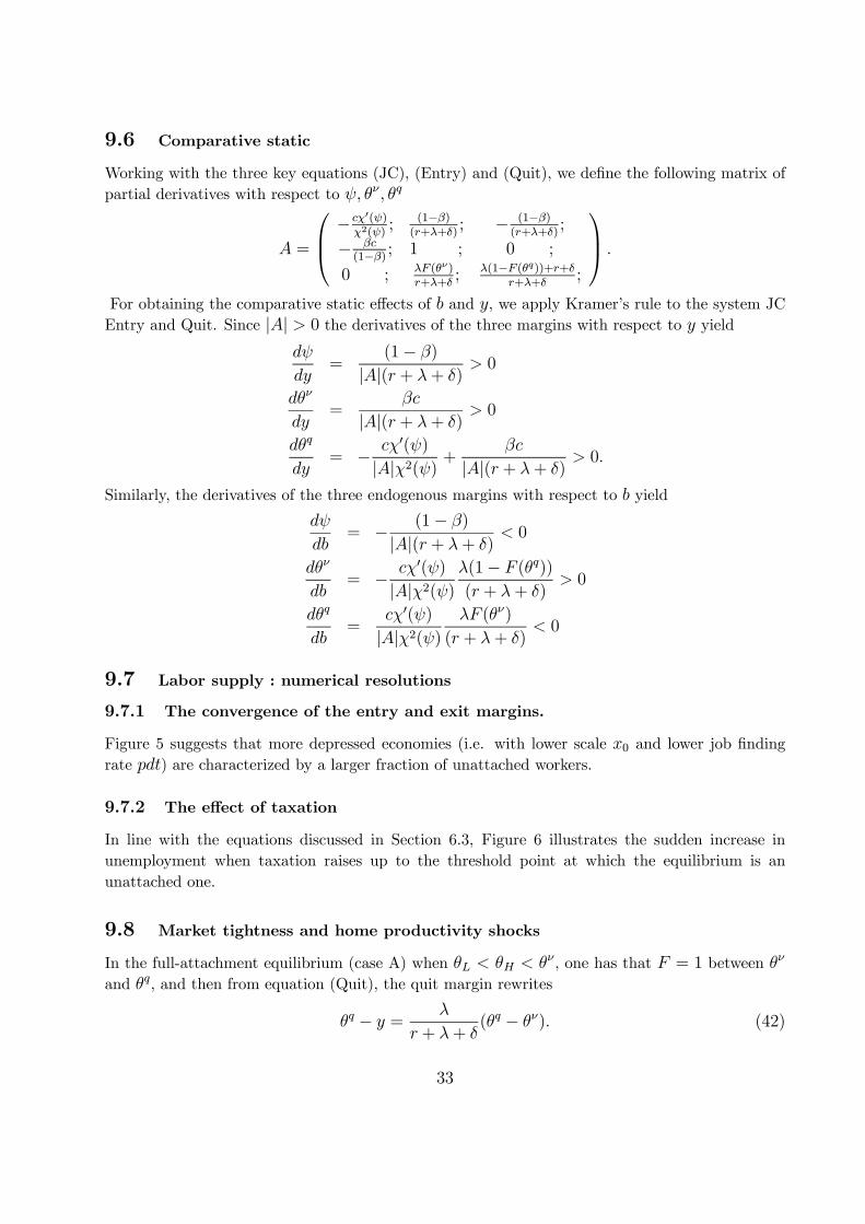
9.6 Comparative static

Working with the three key equations (JC), (Entry) and (Quit), we define the following matrix of

partial derivatives with respect to ψ, θν , θq

A =

− cχ0(ψ)χ2(ψ)

; (1−β)(r+λ+δ)

; − (1−β)(r+λ+δ)

;

− βc(1−β) ; 1 ; 0 ;

0 ; λF (θν)r+λ+δ

; λ(1−F (θq))+r+δr+λ+δ

;

.

For obtaining the comparative static effects of b and y, we apply Kramer’s rule to the system JC

Entry and Quit. Since |A| > 0 the derivatives of the three margins with respect to y yielddψ

dy=

(1− β)|A|(r + λ+ δ) > 0

dθν

dy=

βc

|A|(r + λ+ δ) > 0dθq

dy= − cχ0(ψ)

|A|χ2(ψ) +βc

|A|(r + λ+ δ) > 0.

Similarly, the derivatives of the three endogenous margins with respect to b yield

dψ

db= − (1− β)

|A|(r + λ+ δ) < 0dθν

db= − cχ0(ψ)

|A|χ2(ψ)λ(1− F (θq))(r + λ+ δ)

> 0

dθq

db=

cχ0(ψ)|A|χ2(ψ)

λF (θν)

(r + λ+ δ)< 0

9.7 Labor supply : numerical resolutions

9.7.1 The convergence of the entry and exit margins.

Figure 5 suggests that more depressed economies (i.e. with lower scale x0 and lower job findingrate pdt) are characterized by a larger fraction of unattached workers.

9.7.2 The effect of taxation

In line with the equations discussed in Section 6.3, Figure 6 illustrates the sudden increase in

unemployment when taxation raises up to the threshold point at which the equilibrium is an

unattached one.

9.8 Market tightness and home productivity shocks

In the full-attachment equilibrium (case A) when θL < θH < θν , one has that F = 1 between θν

and θq, and then from equation (Quit), the quit margin rewrites

θq − y = λ

r + λ+ δ(θq − θν). (42)

33

Figure 5: θυ and θq for different matching scale parameters

Figure 6: Proportional taxation, unattachment, and equilibrium unemployment

34

In the unattachment equilibrium (case B), where θL < θν < θH < θq, one has that F = αLbetween θν and θH and 1 above. From equation (Quit), the quit margin rewrites

θq − y = λ

r + λ+ δ[(θq − θν)− αH(θH − θν)]. (43)

Combining these equations with the two other general equilibrium equations (Entry) and (JC), one

obtains the equation (15) of the text. While equation (15) fully determines the equilibrium market

tightness ψ, the unattachment equilibrium requires also that N(θH) > U(θH) or that

θH > θυ = b+βcψ

1− βThe inverse relationship must hold in the attached equilibrium.

In this discrete version of the model, the unattached equilibrium is thus the solution to

r + δ

1− βc

χ(ψ)+

cβ

(1− β)ψ 1− αH λ

r + λ+ δ= y − b− αH(θH − b) λ

r + λ+ δ(44)

where ψ simultaneously solves

θH > (b+βcψ

1− β ) = θυ (45)

There are three comparative static results. First dψdλ< 0. Differentiating equation (44) with respect

to λ and rearranging yields

[− r + δ1− β

cχ(ψ)

χ(ψ)+

cβ

(1− β)r + λ(1− αH) + δ

r + λ+ δ]dψ

dλ=

(r + δ)αH(r + λ+ δ)2

[b+cβ

(1− β)ψ − θH ].

Making use of equation (45) the result immediately follows. Second dψdθH

< 0. Differentiatingequation (44) with respect to θH and rearranging yields

[− r + δ1− β

cχ(ψ)

χ(ψ)+

cβ

(1− β)r + λ(1− αH) + δ

r + λ+ δ]dψ

dθH= − λαH

r + λ+ δ.

Third dψdαH

< 0.Differentiation equation (44) with respect to αH and rearranging yields

[− r + δ1− β

cχ(ψ)

χ(ψ)+

cβ

(1− β)r + λ(1− αH) + δ

r + λ+ δ]dψ

dαH=

λ

(r + λ+ δ)[b+

cβ

(1− β)ψ − θH ].

Making use of equation (45) the result immediately follows.

The effect of θH on market tightness can be understood by considering θH as a proxy for the

variance of the home productivity shocks on unemployment. As shocks become more dispersed (θHraises relatively to θL ) the cost of unattachment to the firm rises, with adverse effects on vacancy

posting and unemployment. Finally, an increase in αH reduces market tightness, since a higher

number of individuals in the high home productivity state implies a larger number of unattached

workers.

35

A latter result is that, using the non-participation equation (41) in Appendix 9.6 with q = 0and F (θν) = 1 (case A), one obtains n = 0: everyone participates to the labor market. Instead, incase B, when F (θν) = 1− αH , non-participation is defined by

n

1− n =δ

δ + p

αH1− αH −

p

δ + λ.

Noting that ∂n/∂p < 0, ∂n/∂αH > 0 and ∂n/∂p < 0, and using the general equilibrium effects

of ψ in (16), one obtains the following general equilibrium results:

dn

dλ> 0;

dn

dθH> 0;

dn

dαH> 0; if iB = 1.

They imply that labor force participation falls with the arrival rate and the variance of home

productivity shocks, as well as with the proportion of workers in the high home productivity state.

9.9 Asymmetric information

Proof of point 1. The total surplus S(θ) is the sum of the surplus of the firm and of the worker.

In θ = θq, the surplus of the worker is zero by definition. So, S(θ

q) = J(θ

q) = y−w

r+δ+q(θq). It is

therefore sufficient to show that the wage is lower than y. From (20), one has

y − wr + δ + q(θ

q)= −1/∂q(θ

q)

∂w= λf(θ

q)∂θ

q

∂w. (46)

From (19), one has that ∂θq

∂w= 1− λ

r+λ+δF (θ

q) > 0 so y > w and S(θ

q) > 0: there are inefficient

destructions.

Proof of point 2. The dual of point 1 : Since the surplus of workers is decreasing with θ andminimum in θ

q, W (θ)−Max(U,N(θ)) is strictly positive for all θ < θq.

Proof of point 3. From (46), S(θq)→ 0 when λ→ 0.

References

[1] Abraham K.G. and Shimer, R. (2001). “Changes in Unemployment Duration and LaborForce Attachment”, NBER Working Paper 8501

[2] Abowd, J. and Zellner, A. (1985) “Estimating Gross Labor Force Flows”, Journal ofEconomics and Business Statistics 3, no. 3: 254-83.

[3] Atkinson, A.B. and Micklewright J. (1991). “Unemployment Compensation and LaborMarket Transitions: A Critical Review”, Journal of Economic Literature, Vol. XXiX,pp. 1679-1727

[4] Becker G.S.. (1965). “ Theory of the Allocation of Time”, The Economic Journal, No299(LXXV), pp493-517

36

[5] Benhabib J., Rogerson R., and R. Wright (1991) “Homework in Macroeconomics:Household Production and Aggregate Fluctuations”, Journal of Political Economy, 99:1166-87.

[6] Ben Porath D. (1967). “The Production of Human Capital and the Life-Cycle of Earn-ings”, Journal of Political Economy, 75:352

[7] Blanchard O.J. , Diamond P. (1990). “The Cyclical Behavior of the Gross Flows of USWorkers”, Brooking Papers on Economic Activity 1990:2, p85-155

[8] Boeri, T. and Burda, M. (1999). “Unions in Search Equilibrium”, mimeo, Humboldt-Universitat zu Berlin.

[9] Burda M., Wyplosz C., 1994, ”Gross workers and job flows in Europe”, European Eco-nomic Review 38(6), p1287-1315

[10] Bowden, R. J. (1980), “On the Existence and Secular Stability of u−v Loci”, Economica47, pp35-50, February

[11] Burdett K., (1979), “Search, leisure and individual labor supply”, chapter 8 in Studiesin the Economics of Search, Contributions to Economic Analysis, Tinbergen, Jorgensonand Waelbroeck eds., North-Holland

[12] Burdett K. and Mortensen D.T., (1978), “Labor Supply Under Uncertainty”, in Re-search in Labor Economics, Ehrenberg R.G. ed.

[13] Burdett K., Kiefer N., Mortensen D., Neumann G. (1984), “Earnings, Unemployment,and the Allocation of Time Over Time”, Review of Economic Studies LI, pp559-578

[14] Daveri, F. and G. Tabellini (2000), “Unemployment, growth and taxation in industrialcountries”, Economic Policy, forthcoming.

[15] Eisner, R. (1988) “Extended Accounts for National Income and Product” Journal ofEconomic Literature 1611-84.

[16] Flinn C.J. and Heckman J.J., (1983), “Are Unemployment and Out of the Labor ForceBehaviorally Distinct Labor Force States”, Journal of Labor Economics, vol.1(1), pp28-42

[17] Garibaldi P. and Wasmer E. (2000). ”Unattachment to the labor market when searcheffort e < 1”, technical Appendix, mimeo ECARES and Bocconi.

[18] Harsanyi J.C. and Selten, R. (1972). ”A Generalized Nash Solution for Two-PersonBargaining Games with Incomplete Information”,Management Science, Vol. 18(5), Jan-uary.

[19] Layard R., Nickell S., and Jackman R., 1991, Unemployment, Oxford, Basil Blackwell

37

[20] Juhn C., Murphy, K. and Topel R.H. (1991). ”Why Has the Natural Rate of Unemploy-ment Increased over Time?”, Brookings Papers on Economic Activity ;0(2), 1991, pp.75-126

[21] McKenna, C.J. (1987), “Labour Market Participation in Matching Equilibrium”, Eco-nomica 54, pp325-333

[22] Mortensen, D.T. and Pissarides, C.A. (1994). “Job Creation and Job Destruction in theTheory of Unemployment”, Review of Economic Studies, 64, 397-415

[23] Mortensen, D.T. and Pissarides, C.A. (1999). “Job Reallocation, Employment Fluctu-ations and Unemployment”, Handbook of Macroeconomics, vol 3B, Ch. 39

[24] Murphy K. and Topel R. H. (1997). ”Unemployment and Nonemployment”, AmericanEconomic Review ; 87(2), May 1997, pp. 295-300

[25] Nickell, S. and Layard, R. (1999) “Labor Market Institutions and Economic Perfor-mance”, in O. Ashenfelter and D. Card eds. Handbook of Labor Economics, Vol 3c.chapter 46 3029-3084

[26] Rogerson, (1988) “Indivisible Labor, Lotteries and Equilibrium”, Journal of MonetaryEconomics 21: 3-16.

[27] OECD (1999). Benefit Systems and Work Incentives. OECD, Paris.

[28] Pissarides C.A. (1990), Equilibrium Unemployment Theory, Oxford, Basil Blackwell

[29] Pissarides C.A. (1998) “The impact of employment tax cuts on unemployment andwages; the role of unemployment ebenfits and tax structure”, European Economic Re-view, vol. 42, pp. 155-83.

[30] Pissarides, C. (2000), Equilibrium Unemployment Theory, Cambridge (MA.): The MITPress.

[31] Sattinger M. (1995), “General Equilibrium Effects of Unemployment Compensationwith Labor Force Participation”, Journal of Labor Economics, vol.13(4), pp623-652

[32] Scarpetta, S. (1996), “Assessing the role of labour market policies and institutionalsettings on unemployment: a cross country study”, OECD Economic Studies 26: 43-98

[33] Seater J.J., (1977), “A Unified Model of Consumption, Labor Supply, and Job Search”,Journal of Economic Theory 14, pp349-372

[34] Sorrentino C. (1993). “International comparisons of unemployment indicators“,MonthlyLabor Review, March.

[35] Sorrentino C. (1995). “International unemployment indicators, 1983-93“,Monthly LaborReview, August.

38

[36] Swaim P. and Podgursky, M. (1994), “Female Labor Supply following Displacement: ASplit-Population Model of Labor Force Participation and Job Search”, Journal of LaborEconomics, vol.12(4), pp640-656

[37] Wasmer, E. (1997). ”Trends in the Workers Flows and Some Consequences on Un-employment: France 1968-1993”, Discussion Paper DELTA 97-14 and Chapter 1 in’Changes in the Composition of the Labor Force. Consequences for Wages and Employ-ment’, unpublished PhD Dissertation, London School of Economics, December 1997.

[38] Weiss, Y. (1986). “The Determination of Life-Cycle Earnings: A survey”, Ch. 11 inHandbook of Labor Economics, Vol. 1, O. Ashenfelter and R. Layard, eds.

39

IZA Discussion Papers No.

Author(s) Title

Area Date

391

J. T. Addison P. Teixeira

Employment Adjustment in Portugal: Evidence from Aggregate and Firm Data

1 11/01

392

P. Tsakloglou F. Papadopoulos

Identifying Population Groups at High Risk of Social Exclusion: Evidence from the ECHP

3 11/01

393

S. M. Fuess, Jr.

Union Bargaining Power: A View from Japan

2 11/01

394

H. Gersbach A. Schniewind

Awareness of General Equilibrium Effects and Unemployment

2 11/01

395

P. Manzini C. Ponsatí

Stakeholders, Bargaining and Strikes 6 11/01

396

M. A. Shields S. Wheatley Price

Exploring the Economic and Social Determinants of Psychological and Psychosocial Health

5 11/01

397

M. Frondel C. M. Schmidt

Evaluating Environmental Programs: The Perspective of Modern Evaluation Research

6 11/01

398

M. Lindeboom F. Portrait G. J. van den Berg

An Econometric Analysis of the Mental-Health Effects of Major Events in the Life of Elderly Individuals

5 11/01

399

J. W. Albrecht J. C. van Ours

Using Employer Hiring Behavior to Test the Educational Signaling Hypothesis

1 11/01

400

R. Euwals

The Predictive Value of Subjective Labour Supply Data: A Dynamic Panel Data Model with Measurement Error

5 11/01

401

J. Boone P. Fredriksson B. Holmlund J. C. van Ours

Optimal Unemployment Insurance with Monitoring and Sanctions

3 11/01

402

O. Ashenfelter D. Card

Did the Elimination of Mandatory Retirement Affect Faculty Retirement Flows?

5 11/01

403

L. Ljungqvist How Do Layoff Costs Affect Employment? 1 11/01

404

H. Battu C. R. Belfield P. J. Sloane

Human Capital Spill-Overs Within the Workplace

1 11/01

405

L. Locher Testing for the Option Value of Migration 3 11/01

406

P. Garibaldi E. Wasmer

Labor Market Flows and Equilibrium Search Unemployment

1 11/01

An updated list of IZA Discussion Papers is available on the center‘s homepage www.iza.org.