labor market policies and job search - connecting … · labor market policies and job search ... i...
TRANSCRIPT

Labor market policies and job search
Paul Muller
2A sizable share of unemployment can be attributed to frictions in the labor market. The simultaneous existence of vacancies and job seekers proves that job search requires effort and time. To improve the efficiency of this process, many countries offer active labor market policies. Evaluating how these programs affect job prospects of job seekers is crucial for effective policy making and forms the basis of this thesis.
Chapter 2 compares different methods to assess the effect of such programs on job finding of participants. Chapter 3 describes a field experiment to investigate how job search strategies and labor market outcomes are affected by the provision of detailed labor market statistics. Chapter 4 examines the possibility that activation programs affect non-participating job seekers through general equilibrium effects. Chapter 5 has a slightly different focus and studies the relation between childcare subsidies and female labor supply.
Paul Muller (1986) obtained his Bachelor degree in economics from the University of Amsterdam in 2008. He followed the MPhil program at the Tinbergen Institute and wrote his Ph.D. thesis at the Vrije Universiteit in Amsterdam. He is currently working as a postdoctoral researcher at the University of Gothenburg.
635
Vrije Universiteit Amsterdam
Labor market policies and job search Paul M
uller

Labor market policies and job search

ISBN 978 90 5170 724 3
Cover design: Crasborn Graphic Designers bno, Valkenburg a.d. Geul
This book is no. 635 of the Tinbergen Institute Research Series, established through
cooperation between Thela Thesis and the Tinbergen Institute. A list of books which
already appeared in the series can be found in the back.

VRIJE UNIVERSITEIT
LABOR MARKET POLICIES AND JOB SEARCH
ACADEMISCH PROEFSCHRIFT
ter verkrijging van de graad Doctor aan
de Vrije Universiteit Amsterdam,
op gezag van de rector magnificus
prof.dr. V. Subramaniam,
in het openbaar te verdedigen
ten overstaan van de promotiecommissie
van de Faculteit der Economische Wetenschappen en Bedrijfskunde
op dinsdag 19 januari 2016 om 13.45 uur
in de aula van de universiteit,
De Boelelaan 1105
door Paul Muller
geboren te Groningen

promotoren: prof.dr. B. van der Klaauw
prof.dr. P.A. Gautier

Acknowledgements
Acknowledgments for this thesis should, without a doubt, start by thanking my
advisers Pieter Gautier and Bas van der Klaauw. Over the course of four years, I have
become aware that your supervision has been extraordinary. You’ve been extremely
accessible and always offered a very relaxed style of guiding me through the process of
producing papers. You were critical when necessary, but mostly very supportive. Your
encouragement to visit conferences and present my work even at an early stage has
proven very beneficial. Finally you have been a great help and support during the job
market in the final year. And maybe equally important, you have broad interests and
were just a lot of fun to be around during coffee breaks, lunches, dinners or even football
matches. This thesis would never have reached this stage without your commitment.
The 5th chapter of this thesis is the result of a fruitful collaboration at the CPB. I
am grateful to my co-authors Egbert Jongen and Leon Bettendorf for making me feel at
home when staying at the CPB. I think we were a good team, and I learned a lot from
you. The experience of doing research which was close to the policy making process
has been very valuable.
For the 3rd chapter I am highly indebted to Philipp Kircher and Michèle Belot. I
am grateful for your invitation to come to the University of Edinburgh for an academic
visit. During my series of visits of in total 9 months, you made sure I felt welcome both
at the department and in Edinburgh. Setting up the experiment has been a difficult,
but ultimately very rewarding experience. Both of you have been inspirational and
your excitement about research has been a major factor in my decision to continue
working in the academic world. The study would not have been possible without the
cooperation from the Job Centres, which is gratefully acknowledged. I would also like
to thank everyone at the economics department for being so welcoming, in particular
Ludo, Jan, Steven, Nick and Mike. Furthermore, the lab team did an amazing job at
organizing the study, while also being great company to spend the many session days
with. Finally I am thankful to Davide, my flatmate in Edinburgh, for mixing the working

hours with very enjoyable Italian dinners as well as the occasional football match or
swing dancing session.
I am thankful to Michael Rosholm and Michael Svarer for their willingness to
collaborate on a project using data from their experiment in Denmark, which led
to the 4th chapter of this thesis. The project leading to chapter 2 would not have been
possible without the support of the UWV, which granted us access to their dataset on
Dutch UI benefit receivers. I am thankful to Arjan Heyma for agreeing to jointly exploit
this dataset.
To my office mates at the VU (in the first 3 years), Łukasz and Lisette, I owe a lot. I
need to thank you for countless interesting or less interesting discussions, gossips and
polish lessons. Most importantly, you became great friends and you made coming to
the VU each morning a pleasure rather than an obligation. To Dennis, you turned out
to be the perfect friend at work. We have lots in common and shared many excitements
as well as doubts about academic research, while our boxing sessions were a great relief
after (sometime frustrating) working days. I am very glad that you agreed to be my
paranymph. I am sad to leave the economics department of the VU, as it has always
been a great pleasure to be there. The atmosphere is so relaxed, while at the same time
encouraging and stimulating. I would like to thank all colleagues, and in particular
Xiaoming, Sandra, Nahom, Maarten, Gosia, Nynke, Sabien, José Luis, Jochem, Sándor
and Luca.
I am thankful to Hessel Oosterbeek and Erik Plug for sparking my interest in the
search for causal effects through their master’s course and for stimulating me to enroll
in the Mphil program of the Tinbergen Institute. I would like to thank the reading
committee for taking their time to go through this entire thesis and providing useful
feedback. José Luis has provided invaluable advice during the search for an academic
position in the last year. The introduction of this thesis benefited a lot from feedback
from Sandra. Thanks to Sietske for her help with finding a front cover picture.
Rogier, thanks for being such a great friend ever since the time I moved to Ams-
terdam, and for now agreeing to be my paranymph. I have greatly appreciated the
many hours I spend with Bastian in the first years at the Tinbergen Institute, either
studying or in the gym, and later on the many interesting discussions we had about
research and other things. Furthermore, I’d like to thank all my friends in Amsterdam,
Zwolle and other places for providing so many great and necessary distractions from
work. To my family, Marten, Carla, Arjan, Sietske, Thom and Eric, I am grateful for your
unconditional support and interest in what I have been working on.

Pursuing a Phd has been a great choice for one final reason. Nadine, we started
out as colleagues, but the last few years we have shared so many experiences. You
are a wonderfully kind and enthusiastic person and your curiosity and openness to
everything in life is unsurpassed. I feel lucky and grateful to spend our lives together
and to start a new adventure with you in Sweden.

Contents
1 Introduction 1
2 Comparing methods to evaluate the effects of job search assistance 5
2.1 Introduction . . . . . . . . . . . . . . . . . . . . . . . . . . . . . . . . . . . 5
2.2 Literature . . . . . . . . . . . . . . . . . . . . . . . . . . . . . . . . . . . . . 8
2.3 Institutional setting and the policy discontinuity . . . . . . . . . . . . . . 9
2.4 Data . . . . . . . . . . . . . . . . . . . . . . . . . . . . . . . . . . . . . . . . 11
2.5 Treatment effects . . . . . . . . . . . . . . . . . . . . . . . . . . . . . . . . 16
2.5.1 Defining the treatment effect . . . . . . . . . . . . . . . . . . . . . 16
2.5.2 Identification . . . . . . . . . . . . . . . . . . . . . . . . . . . . . . 20
2.5.3 Business cycle, seasonalities and cohort composition . . . . . . 21
2.6 Quasi-experimental analysis . . . . . . . . . . . . . . . . . . . . . . . . . . 24
2.6.1 Intention-to-treat effect . . . . . . . . . . . . . . . . . . . . . . . . 25
2.6.2 Average treatment effect . . . . . . . . . . . . . . . . . . . . . . . . 27
2.6.3 Common trend assumption . . . . . . . . . . . . . . . . . . . . . . 29
2.7 Non-experimental analysis . . . . . . . . . . . . . . . . . . . . . . . . . . . 30
2.7.1 Matching . . . . . . . . . . . . . . . . . . . . . . . . . . . . . . . . . 30
2.7.2 Timing of events model . . . . . . . . . . . . . . . . . . . . . . . . 34
2.8 Discussion . . . . . . . . . . . . . . . . . . . . . . . . . . . . . . . . . . . . 37
2.9 Conclusion . . . . . . . . . . . . . . . . . . . . . . . . . . . . . . . . . . . . 39
3 Providing advice to job seekers at low cost: An experimental study on on-
line advice 41
3.1 Introduction . . . . . . . . . . . . . . . . . . . . . . . . . . . . . . . . . . . 41
3.2 Related Literature . . . . . . . . . . . . . . . . . . . . . . . . . . . . . . . . 47
3.3 Institutional Setting . . . . . . . . . . . . . . . . . . . . . . . . . . . . . . . 50
3.4 Experimental Design . . . . . . . . . . . . . . . . . . . . . . . . . . . . . . 52

3.4.1 Basic setup . . . . . . . . . . . . . . . . . . . . . . . . . . . . . . . . 52
3.4.2 Recruitment Procedure and Experimental Sample . . . . . . . . 52
3.4.3 Study Procedure . . . . . . . . . . . . . . . . . . . . . . . . . . . . 54
3.4.4 Experimental Treatments . . . . . . . . . . . . . . . . . . . . . . . 55
3.5 Background Data on our Sample . . . . . . . . . . . . . . . . . . . . . . . 61
3.5.1 Representativeness of the sample . . . . . . . . . . . . . . . . . . 61
3.5.2 Treatment and Control Groups . . . . . . . . . . . . . . . . . . . . 65
3.5.3 Attrition . . . . . . . . . . . . . . . . . . . . . . . . . . . . . . . . . 66
3.5.4 Measuring occupational and geographical broadness . . . . . . 67
3.6 Empirical Analysis . . . . . . . . . . . . . . . . . . . . . . . . . . . . . . . . 68
3.6.1 Econometric specification . . . . . . . . . . . . . . . . . . . . . . . 69
3.6.2 Effects on Listed vacancies . . . . . . . . . . . . . . . . . . . . . . 72
3.6.3 Effects on Applications . . . . . . . . . . . . . . . . . . . . . . . . . 75
3.6.4 Effects on interviews . . . . . . . . . . . . . . . . . . . . . . . . . . 77
3.7 An Illustrative Model . . . . . . . . . . . . . . . . . . . . . . . . . . . . . . 84
3.8 Conclusion . . . . . . . . . . . . . . . . . . . . . . . . . . . . . . . . . . . . 90
3.9 Appendix . . . . . . . . . . . . . . . . . . . . . . . . . . . . . . . . . . . . . 91
3.9.1 Extended results . . . . . . . . . . . . . . . . . . . . . . . . . . . . 91
4 Estimating equilibrium effects of job search assistance 97
4.1 Introduction . . . . . . . . . . . . . . . . . . . . . . . . . . . . . . . . . . . 97
4.2 Background . . . . . . . . . . . . . . . . . . . . . . . . . . . . . . . . . . . . 99
4.2.1 The Danish experiment . . . . . . . . . . . . . . . . . . . . . . . . 99
4.2.2 Treatment externalities . . . . . . . . . . . . . . . . . . . . . . . . 102
4.3 Data . . . . . . . . . . . . . . . . . . . . . . . . . . . . . . . . . . . . . . . . 105
4.4 Estimations . . . . . . . . . . . . . . . . . . . . . . . . . . . . . . . . . . . . 110
4.4.1 Unemployment durations . . . . . . . . . . . . . . . . . . . . . . . 110
4.4.2 Earnings and hours worked . . . . . . . . . . . . . . . . . . . . . . 117
4.4.3 Vacancies . . . . . . . . . . . . . . . . . . . . . . . . . . . . . . . . 117
4.5 Equilibrium analysis of the activation program . . . . . . . . . . . . . . . 120
4.5.1 The labor market . . . . . . . . . . . . . . . . . . . . . . . . . . . . 120
4.5.2 Wages and the matching function . . . . . . . . . . . . . . . . . . 123
4.5.3 Equilibrium and welfare . . . . . . . . . . . . . . . . . . . . . . . . 125
4.6 Estimation and evaluation . . . . . . . . . . . . . . . . . . . . . . . . . . . 127

4.6.1 Parameter values . . . . . . . . . . . . . . . . . . . . . . . . . . . . 127
4.6.2 Increasing the intensity of the activation program . . . . . . . . . 130
4.6.3 Robustness checks . . . . . . . . . . . . . . . . . . . . . . . . . . . 133
4.7 Conclusion . . . . . . . . . . . . . . . . . . . . . . . . . . . . . . . . . . . . 138
4.8 Appendix . . . . . . . . . . . . . . . . . . . . . . . . . . . . . . . . . . . . . 140
4.8.1 Empirical analyses with restricted comparison counties . . . . . 140
4.8.2 Equilibrium search model with Bertrand competition . . . . . . 140
5 Childcare subsidies and labor supply - Evidence from a large Dutch reform 145
5.1 Introduction . . . . . . . . . . . . . . . . . . . . . . . . . . . . . . . . . . . 145
5.2 The reform . . . . . . . . . . . . . . . . . . . . . . . . . . . . . . . . . . . . 148
5.3 Methodology . . . . . . . . . . . . . . . . . . . . . . . . . . . . . . . . . . . 156
5.4 Data . . . . . . . . . . . . . . . . . . . . . . . . . . . . . . . . . . . . . . . . 158
5.5 Estimation results . . . . . . . . . . . . . . . . . . . . . . . . . . . . . . . . 162
5.5.1 Participation rate . . . . . . . . . . . . . . . . . . . . . . . . . . . . 162
5.5.2 Hours worked per week . . . . . . . . . . . . . . . . . . . . . . . . 165
5.5.3 Results for men . . . . . . . . . . . . . . . . . . . . . . . . . . . . . 168
5.6 Discussion . . . . . . . . . . . . . . . . . . . . . . . . . . . . . . . . . . . . 169
5.7 Conclusion . . . . . . . . . . . . . . . . . . . . . . . . . . . . . . . . . . . . 173
6 Summary and Conclusions 177
Bibliography 181
Samenvatting (Dutch summary) 193

CHAPTER 1Introduction
A sizeable share of unemployment can be attributed to frictions in the labor market.
The simultaneous existence of vacancies and job seekers proves that job search requires
effort and time. Vacancies need to be identified, applications have to be written,
candidates have to be selected. Government policies, in particular unemployment
insurance and activation programs, play a large role in this process. Unemployment
insurance insures workers against the lack of income during periods of unemployment,
though it may also create a moral hazard problem by lowering the incentives to search
for a job. Incentive schemes consisting of decreasing benefits over time, job search
effort monitoring and sanctions, are commonly used policies to solve this problem. To
improve the efficiency of the matching process, many countries also offer active labor
market policies (ALMP), such as job search assistance, training programs, schooling
or subsidized employment. In most developed countries, such programs represent a
large share of the government’s budget: around 0.5% of GDP (OECD (2010)). Many
different types of programs have been suggested or implemented such that a large range
of options exist for policy makers. Reliable estimates of the benefits of these programs
are therefore necessary.
The literature investigating the effects of ALMP’s is large and has reached some
consensus on the effectiveness of particular programs (see the meta-analysis by Card
et al. (2010)). Such evaluation studies have to deal with the fact that participants in a
program are typically a very selective group. Participants are either selected by case
workers, or they select themselves by volunteering because they are highly motivated to

2 1. Introduction
find a job. In both cases, they differ from the average job seeker in many dimensions. For
example, if they are selected by case workers, they are probably less able or motivated to
find employment than the average job seeker. This leads to a bias if one would estimate
the effect of the program by comparing participants and non-participants. Controlling
for many observable characteristics could solve the problem, though it is impossible to
determine whether no unobserved differences remain.
In chapter 2 of this thesis, evaluation methods for job search assistance programs
are compared to assess the magnitude of the selection problem. First, the effect
of an intensive activation program in the Netherlands on job finding is estimated
using a discontinuity in the provision of the program. The discontinuity provides
exogenous variation in the provision of the program, such that it can be used as a
natural experiment to identify how the program affects job finding. The results are then
compared to non-experimental estimates (using cross sectional data) to assess to what
extent selection based on unobservable characteristics affects the estimates of program
impacts. First, the study finds that the activation program was ineffective in guiding job
seekers to work. Results even suggest that, in the short-run, the program reduces job
finding. Second, the non-experimental estimates underestimate the effect significantly:
they suggest that the program reduces job finding even in the long-run. The difference
in findings implies that program participants have, on average, ’worse’ unobserved
characteristics than the average job seeker, leading to worse job finding prospects. This
difference remains even after correcting for a large set of observed characteristics.
While many studies have estimated the effects of ALMP’s on job finding (or on the
quality of the new job), a number of other angles have received relatively little attention.
Mostly because of the lack of necessary data, little is known about the job search
strategies of unemployed individuals. Moreover, how job search strategies change as
a result of job search assistance programs has hardly been investigated. Job seekers
may start sending out more applications. The quality of applications may improve. Job
seekers might be induced to search in a broader set of occupations or focus on one
specific one. Job seekers may simply dislike participating in a program and as a result
they might search more or become less picky (lower their reservation wage) in order to
be able to leave the program. This mechanism is often referred to as the ’threat effect’.
The mechanisms behind changes in job finding rates have remained somewhat of a
black box. While rich administrative data is nowadays available on unemployment
duration, employment histories and job finding, it is difficult to observe unsuccessful
applications.

3
Chapter 3 focuses on job search strategies of unemployed workers. It reports results
from a controlled experiment in which job seekers were followed for 12 weeks, while
spending a minimum of 30 minutes per week searching for jobs in the behavioral
lab of the University of Edinburgh. The designed job search engine recorded all job
search details and in addition performed a weekly survey to obtain many background
characteristics as well as information on other channels of job search. A randomized
trial among the participants presented half of the participants with an alternative search
interface, which provided information on suitable occupations based on their preferred
occupation. It also presented geographical information on labor market tightness. The
setup of the study allows to observe job search strategies in great detail: which criteria
are used when performing an online search, which vacancies are saved as interesting,
which are applied to, which lead to a job interview. The results of the study show that
providing information is beneficial for job seekers that search “narrow” in terms of
occupations and have been unemployed for more than two and a half months. For
this group the intervention led to a broader search strategy in terms of occupations,
and increased the number of job interviews. Since the intervention is relatively cheap
(especially compared to frequent meetings with a case worker or training programs),
the finding of a positive effect is particularly interesting from a policy perspective. The
rich set of information resulting from this study shall be used in the future to address
other questions related to job search strategies as well.
One could argue that the effect of a program on job finding is all that matters,
and the mechanism is of second order importance. That this is not the case, is
demonstrated in chapter 4 of this thesis, which evaluates a job search assistance
program that was offered in two regions in Denmark. Conventional evaluation studies
have shown that participants of this program found jobs quicker than non-participants
(Graversen and van Ours (2008), Rosholm (2008)). However, since it is unknown how the
program increases the job finding rate, we cannot conclude that the program increases
welfare. The higher job finding rate could result from different mechanisms: more
applications, better applications, an improvement of skills (productivity), a decrease
of the reservation wage or an increase in job seekers abilities to find vacancies that
suit best their skills and preferences. Some of these mechanisms may imply that the
increased job finding of participants comes at the expense of other job seekers. For
example, if those that follow the program double their number of applications, they will
find jobs quicker, but this is likely to reduce job finding of other job seekers.

4 1. Introduction
Whether such externalities occur, is investigated in chapter 4. Using a difference-
in-differences approach we compare randomly selected participants in the job search
assistance program with randomly selected non-participating job seekers in the same
region, but also with job seekers in other regions. We find that while participants
are more successful in finding jobs after the introduction of the program, the non-
participants in the same region were less successful. Crowding out seems to be
important: the success of the participants comes at the expense of the non-participants.
The second part of the chapter uses these findings to estimate a structural search model
to simulate the policy relevant outcomes when the program would rolled out on a large
scale. These results suggest that if all job seekers would participate in the program,
there would be no effect on job finding. Therefore, a large scale roll-out of the program
would reduce welfare.
The 5th chapter of this thesis looks at a different type of labor market policy: it
investigates whether childcare subsidies incentivize mothers with young children to
increase their labor supply. Childcare subsidies were increased substantially in the
Netherlands in 2005 and they were also extended to home care. For most families, this
led to a sizeable decrease in the costs of childcare, thereby increasing the returns to
employment. This policy reform is exploited to estimate the labor supply response of
mothers with young children. We find that the participation rate of mothers increased
slightly (the extensive margin), while a larger effect is found for the number of hours
worked per week (the intensive margin). The magnitude of the increase is small
compared to the budgetary impulse: we compute that the cost in terms of extra
subsidies of each additional full-time job is around 90,000 Euro.
Chapter 6 concludes, and provides a summary of all chapters.

CHAPTER 2Comparing methods to evaluate
the e�ects of job search
assistance1
2.1 Introduction
In 2002 the Dutch market for job search assistance programs was privatized, implying
that the unemployment insurance (UI) administration buys services of private com-
panies to help benefits recipients in their job search. Due to the economic crisis the
demand for programs increased sharply in 2009 and early 2010. This caused budgetary
problems in March 2010 and the government refused to extend the budget. As a result,
the purchase of new programs was terminated within a period of two weeks. During the
remainder of the year, new UI benefits recipients could not enroll in these programs
anymore. In this paper we exploit this policy discontinuity to evaluate the effects of the
programs on job finding. We then estimate the same effects using non-experimental
methods and assess their performance using the quasi-experimental estimates as a
benchmark.
The main challenge faced when evaluating activation programs is selective participa-
tion (Heckman et al. (1999), Abbring and Heckman (2007)). As shown in a meta-analysis
by Card et al. (2010), over 50% of the evaluation studies use longitudinal data and
1This chapter is based on Muller et al. (2015)

6 2. Comparing methods
compare a treatment group with a control group, where the control group is typically
formed by matching on observable characteristics. Over one-third of the studies use
duration models. Less than 10% of the studies use an experimental design. In his
seminal study, LaLonde (1986) shows that non-experimental estimators produce results
that do not concur with those from experimental evidence. In an extension Dehejia
and Wahba (1999) test the performance of matching estimators, finding that those are
closer to the experimental evidence. Their findings are however disputed by Smith
and Todd (2005), who evaluate the same program and show that the findings are not
robust to different specifications and to the use of different samples and different sets of
covariates. They refer to Heckman et al. (1997) who argue that matching estimators can
only replicate experimental findings if three requirements are fulfilled. First, the same
data source for treated and control group should be used (in particular the outcome
variable should be measured in the same way). Second, treated and control individuals
should be active in the same local labor market. Third, the data should contain a rich set
of variables that affect both program participation and labor market outcomes. Smith
and Todd (2005) state that each of these requirements is likely to be violated in the
evaluations by LaLonde (1986) and Dehejia and Wahba (1999). However, since the
1970’s data quality has improved, as well as statistical methods.
We build on this literature by performing a similar comparison of methods, using a
recent, rich administrative dataset. Our main contribution is twofold. First, since our
quasi-experimental estimates are identified from a large scale policy discontinuity in
2010 in the Netherlands, the setting is particularly suitable for such a comparison. Our
data fulfills the criteria mentioned by Smith and Todd (2005). The administrative dataset
allows the use of high-quality information on a rich set of variables, including individual
characteristics, pre-unemployment labor market variables, current unemployment
spell characteristics and any assistance provided by the UI administration and private
providers. As the policy discontinuity was nationwide, the sample size is substantial.
Since the policy discontinuity occurred recently, programs and labor market conditions
are similar to those currently in many countries. Second, for the non-experimental
analysis we not only apply a range of matching estimators, but also estimate the timing-
of-events model. This allows us to compare both approaches to our baseline estimates
and assess which performs best.
We exploit the policy discontinuity to non-parametrically estimate how program
participation affects job finding. The variation in program provision due to the quasi-
experiment is large. Within a month, the weekly number of new program participants

2.1. Introduction 7
dropped from 1300 to less than 80 and remained below 50 for the remainder of the
year. We estimate the treatment effect on the treated by comparing the job finding
rates of cohorts entering unemployment at different points in time, though relatively
short after each other. Since they reach the discontinuity at different unemployment
durations they are affected differentially. This identifies the effect of the programs.
Seasonal differences in the labor market are controlled for using cohorts from the
previous year. Our results show that after starting a program, the job finding rate is
reduced significantly for several months (i.e. lock-in effect). After half a year it increases,
up to a zero difference in job finding after 12 to 18 months.
We compare these results to several matching estimators (inverse probability
weighting, propensity score matching, regression adjustment and nearest neighbor
matching). Results are very similar across the four matching estimators. All show a
significant negative effect of program participation directly after entry in the program.
Even though the negative effect decreases in magnitude over time, all estimators remain
significantly negative after 18 months. Next, we estimate a timing-of-events model
(Abbring and Van den Berg (2003)), which controls for selection on unobservables by
adding more structure on the model. In particular it jointly models the hazard rate
to employment and the hazard rate to program participation. Using this model we
estimate that the program reduces the job finding rate in the first six months, while it
slightly increases the job finding rate at longer durations. Overall this leads to a negative
effect on employment in the first 14 months, and a zero effect afterwards.
To summarize, all methods find a negative effect in the first couple of months, while
only the quasi-experimental estimates and the timing-of-events model find that the
effect in the medium run is zero. The fact that the matching estimator underestimates
the effect suggests that program participants are a selective group with relatively
unfavorable unobservable characteristics.
The remainder of the paper is structured as follows. We briefly discuss the literature
on the evaluation of active labor market programs in Section 2.2, and describe the
institutional setting and the budgetary problems which led to the policy discontinuity
in Section 2.3. An overview of the data is provided in Section 2.4. In Section 2.5 we define
the treatment effects and discuss how they are identified from the policy discontinuity.
In Section 2.7 we present the quasi-experimental estimation results, while Section 2.7
contains the non-experimental estimation methods and results. Section 2.8 compares
the results from the different methods and provides a discussion. Section 2.9 concludes.

8 2. Comparing methods
2.2 Literature
There is a large literature studying the effectiveness of active labor market programs.
Reviews provided by Kluve (2010) and Card et al. (2010) show that there is some consen-
sus on the effects of different types of programs on post-unemployment outcomes such
as employment, wages and job stability. For example, job search assistance is found to
be more likely to have positive effects on job finding than alternatives such as public
sector employment programs. The surveys emphasize that difference methodologies
are used, but find little evidence that empirical results are related to the methodological
approach.
Card et al. (2010) report that only 9% of the evaluation studies in their meta-analysis
use an experimental approach. For example, Dolton and O’Neill (2002) use random
delays in program participation to assess the effect of a job search assistance program
in the UK. Van den Berg and Van der Klaauw (2006) analyse a randomized experiment
of counseling and monitoring, to show that the program merely shifts job search effort
from the informal to the formal search channel. Graversen and van Ours (2008) evaluate
an intensive activation program in Denmark, using a randomized experiment. Card
et al. (2011) show estimates of the effect of a training program offered to a random
sample of applicants in the Dominican Republic. Behaghel et al. (2014) perform a large
controlled experiment, randomizing job seekers across publicly and privately provided
counseling programs.
Randomized experiments are typically expensive and have practical and ethical
complications. Alternatively, quasi-experimental approaches are often used. Van den
Berg et al. (2014) discuss the use of regression discontinuity with duration data and
apply their approach to the introduction of the New Deal for the Young People in the UK.
Van der Klaauw and Van Ours (2013) analyze the effect of both an employment bonus
and sanctions, exploiting policies changes in the bonus levels. Cockx and Dejemeppe
(2012) use a regression discontinuity approach to estimate the effect of extra job search
monitoring in Belgium.
Many studies use non-experimental methods such as matching. For example,
Brodaty et al. (2002) apply a matching estimator to estimate the effect of activation
programs for long-term unemployed workers in France, Sianesi (2004) investigates
different effects of active labor market programs in Sweden and Lechner et al. (2011)
looks at long-run effects of training programs in Germany. Some other studies applied

2.3. Institutional setting and the policy discontinuity 9
the timing-of-events model (Abbring and Van den Berg (2003)). For example, this model
is used to evaluate the effect of benefit sanctions in the Netherlands (Van den Berg et al.
(2004) and Abbring et al. (2005)) and to evaluate a training program in France by Crépon
et al. (2012).
Some studies compared outcomes of different methods. LaLonde (1986), Dehejia
and Wahba (1999) and Smith and Todd (2005) show how the difference between
experimental and non-experimental estimates can be substantial, using data from
a job training program in the US. More recently, Lalive et al. (2008) evaluate the effect of
activation programs in Switzerland. They find that matching estimators and estimates
from a timing-of-events model lead to different results. Mueser et al. (2007) use a wide
set of matching estimators to estimate the earnings effect of job training programs in the
US. They find that a combination of difference-in-differences and matching performs
best, and produces results that are similar to estimates from a randomized experiment
(Orr et al. (1996)). Kastoryano and Van der Klaauw (2011) evaluate job search assistance
provided in the Netherlands. They compare different methods for dynamic treatment
evaluation (discrete and continuous) and find that results are similar. Biewen et al.
(2014) provide estimates of the effect of training programs. They show that results are
very sensitive to data features and methodological choices.
2.3 Institutional setting and the policy discontinuity
In this section we briefly describe the institutional setting and the policy discontinuity
in program provision.
In the Netherlands unemployment insurance (UI) is organized at the nationwide
level. The UI administration (UWV) pays benefits to all eligible workers. Since October
2006 the eligibility criteria are as follows (see Van der Klaauw and de Groot (2014) for an
extensive discussion). A worker should have involuntary lost at least half of her working
hours with a minimum of five hours per week. The worker should have worked for at
least 26 weeks out of the last 36 weeks. Fulfillment of this "weeks condition" provides a
eligibility to benefits for three months. During the first two months benefits are 75%
of the previous wage, capped at a daily maximum. From the third month onward it is
70% of the previous wage. If the worker has worked at least four out of the last five years,
the benefits eligibility period is extended with one month for each additional year of
employment. The maximum UI benefits duration is 38 months.

10 2. Comparing methods
A UI benefits recipient is required to register at the public employment office, and
to search for work actively. The latter requires making at least one job application
each week. Case workers at the UI administration provide basic job search assistance
through individual meetings, and offer some additional assistance programs. Benefit
recipients are obliged to accept any suitable job offer.2 Case workers are responsible
for monitoring these obligations. In general, the intensity of meetings is low though
(only in case the case worker suspects that a recipient is unable to find work without
assistance a meeting is scheduled). In 2009, case workers had the possibility of assigning
an individual to a range of programs aiming at increasing the job finding rate, if she
judged that the benefits recipient required more than the usual guidance. A large
diversity of programs existed, including job search assistance, vacancy referral, training
in writing application letters and CV’s, wage subsidies, subsidized employment in
the public sector and schooling. Some of these were provided internally by the UI
administration, while others were purchased externally from private companies. Our
analysis focuses on the externally provided programs. These can be broadly classified as
(with relative frequency in parentheses) job search assistance programs (56%), training
or schooling (31%), subsidized employment (2%) and other programs (11%). Though
some guidelines existed, case workers had a large degree of discretion in deciding about
program assignment.
The lack of centralized program assignment together with an increased inflow in
unemployment due to the recession caused that many more individuals were assigned
to these programs in 2009 and early 2010 than the budget allowed. Therefore the
entire budget had been exhausted by March 2010. The authorities declared that no
new programs should be purchased from that moment onward.3 Assistance offered
internally by the UI administration continued without change. In Section 2.4 we show
that indeed the number of new program entrants dropped to almost zero in March 2010
and remained very low for the rest of 2010.
2During the first six months a suitable job is defined as a job at the same level as the previous job,between six and 12 months it can be a job below this level, and after 12 months any job is suitable andshould be accepted.
3This was declared by the minister of social affairs, in a letter to parliament on March 15. An exceptionwas made for a small number of specially targeted programs (mostly for long-term unemployed workers).

2.4. Data 11
2.4 Data
We use a large administrative dataset provided by the UI administration, containing
all individuals who started collecting UI benefits between April 2008 and September
2010 in the Netherlands. The dataset contains 608,998 observations (each UI spell is
considered an observation, though for some individuals there are multiple spells).4
We select a sample of individuals with a high propensity to participate in the external
programs. These are native males, aged 40 to 60 years, with a low unemployment history
(at most two unemployment spells in the past 3 years) and belonging to the upper 60%
of the income distribution in our data. This reduces the sample to 116,866 observations.
The advantage of restricting the sample is twofold. First, the policy discontinuity affects
this group strongest, which strengthens the first stage of the analysis. Second, the
estimates will be more precise when using a homogeneous sample.5
For each spell we observe the day of starting receiving UI benefits and, if the spell
is not right censored, the last day and the reason for the end of the benefit payments.
Right censoring occurs on January 1st, 2012, when our data was constructed, so for each
individual we can observe at least 16 months of benefits receipt. The dataset contains a
detailed description of all activation programs (both internally and externally provided)
in which benefits recipients participated in. Furthermore individual characteristics and
pre-unemployment labor market outcomes are included in the dataset.
Figure 1 shows how the monthly number of individuals entering UI evolves over
time. Due to the economic crisis, there is a substantial increase in the inflow from
December 2008 onward. In particular the inflow increased from about 2000 to 5000
per month and remained high until the end of 2009. From 2010 onward the inflow
decreased somewhat. Table 1 presents summary statistics for the full sample, as well
as for three subgroups defined by their month of inflow into unemployment. Column
(1) shows that for the full sample the median duration of unemployment is 245 days
(around eight months). Almost 60% of those exiting UI find work, while 15% reaches
4The original dataset contains 671,743 unemployment spells. We exclude 35,671 spells fromindividuals previously employed in a government sector and 17,577 from individuals older than 60years. Next, we drop 533 spells from individuals working more than 60 hours or less than 12 hours in theirprevious job and 151 spells from individuals who were eligible for a so-called ’education and developmentfund’. Finally we exclude 8518 spells with a duration of zero days and 290 spells from individuals withinconsistent or missing data (such as a negative unemployment duration). These are often individualsfor whom the application to benefits was later denied.
5For example, using a homogeneous sample improves the performance of the matching estimatorsthat we applied in Section 2.7.1 (Imbens (2014)).

12 2. Comparing methods
Table 1: Descriptive statistics
Inflow cohort UI:Full April April April
sample 2008 2009 2010Unemployment duration (median, days) 245 175 280 275Reason for exit (%):
Work 57.2 52.3 52.5 62.2End of entitlement period 15.4 21.5 19.1 8.3Sickness/Disability 6.7 6.2 7.3 7.6Unknown 12.9 12.2 12.8 12.6Other 7.8 7.8 8.3 9.3
Participation external program (%):Any program 18.7 24.0 32.3 0.7
Job search assistance 11.0 17.1 21.3 0.3Training 6.0 7.3 9.7 0.2Subsidized employment 0.4 0.3 0.8 0.0Other 4.9 4.4 7.7 0.2
Participation internal program (%):Any program 36.8 13.5a 40.8 39.2
Job search assistance 11.6 1.7a 12.1 13.6Subsidized employment 3.2 1.1a 3.9 3.8Tests 9.7 1.9a 10.3 10.9Workshop entrepreneurship 4.4 2.3a 6.3 3.4Other 19.7 9.1a 23.4 19.6
Gender (% males) b 100 100 100 100Immigrant (%)b 0.0 0.0 0.0 0.0Previous hourly wage (%):
Lowb 0.0 0.0 0.0 0.0Middle 57.4 53.8 58.3 53.1High 42.6 46.2 41.7 46.9
Age 48.7 49.0 48.6 48.9Unemployment size (hours) 37.2 37.1 37.4 37.3UI history last 3 year (%) 29.2 33.8 28.8 23.3Education (%):
Low 22.8 20.0 21.6 20.5Middle 46.5 43.0 45.7 47.1High 30.7 37.1 32.7 32.4
Observations 116,866 1774 4441 4505
Job search assistance contains ’IRO’, ’Jobhunting’ and ’Application letter’. Training contains
’Short Training’ and ’Schooling’. Subsidized employment contains ’Learn-work positions’. a
Biased downwards, because participation in internal programs was rarely recorded before 2009.b Used to select the sample.

2.4. Data 13
Figure 1: Entrants in UI benefits per month0
200
040
00
60
00
Nu
mb
er
of
ne
w s
pe
lls
2008m1 2008m7 2009m1 2009m7 2010m1 2010m7Starting month
the end of their benefits entitlement period. Almost 7% leave unemployment due to
sickness or disability, the rest leave for other reasons (mostly right-censoring) or the
reason for exit is unknown. Exits due to reaching the end of ones entitlement period and
exits due to sickness or disability are unlikely to be affected by program participation
(and are in any case not outcomes of interest). Therefore we focus on exits to work and
exits due to unknown reasons (these may often include situations in which workers
generate some income from other sources than employment).
In the full sample about 19% participate in one of the externally provided programs.
Two-thirds of these programs focus on job search assistance, a third involve some sort
of training, while only a very small fraction are subsidized employment. About 37% of
all individuals participate in an internal program, of which the majority is either some
test (such as a competencies test) or job search assistance.
The dataset contains a large set of individual characteristics, including gender,
age, immigrant status, education level, previous hourly wage, unemployment size,

14 2. Comparing methods
Figure 2: Number of UI benefits recipients entering the external programs per month0
1000
2000
3000
Num
ber
of p
rogr
am s
tart
s
2008m1 2009m1 2010m1 2011m1Starting month program
occupation in previous job, unemployment history, region and industry. In the lower
panel of Table 1 mean values are presented for some characteristics. The average
individual is almost full-time unemployed (37.2 hours) and 29% have experienced some
period of unemployment in the three years before entering UI.
In columns (2), (3) and (4) the same statistics are presented for three subgroups of
individuals entering unemployment in April 2008, April 2009 and April 2010, respectively.
The impact of the policy discontinuity in March 2010 becomes clear from the share of
the April 2010 group that participates in an external program. It drops to almost zero. To
illustrate the impact of the discontinuity in March 2010, we show the number of external
programs started per month in Figure 2. The dashed line indicates the moment of the
policy change in March 2010. The number of program entrants drops to almost zero in
April 2010. Separate graphs for each type of program can be found in the appendix of
Muller et al. (2015) and show that the discontinuity occurs for each type of program.
The calendar date of entry in UI determines how the policy change affected
individuals. Figure 3 shows for the different inflow cohorts the weekly probability
2.4. Data 15
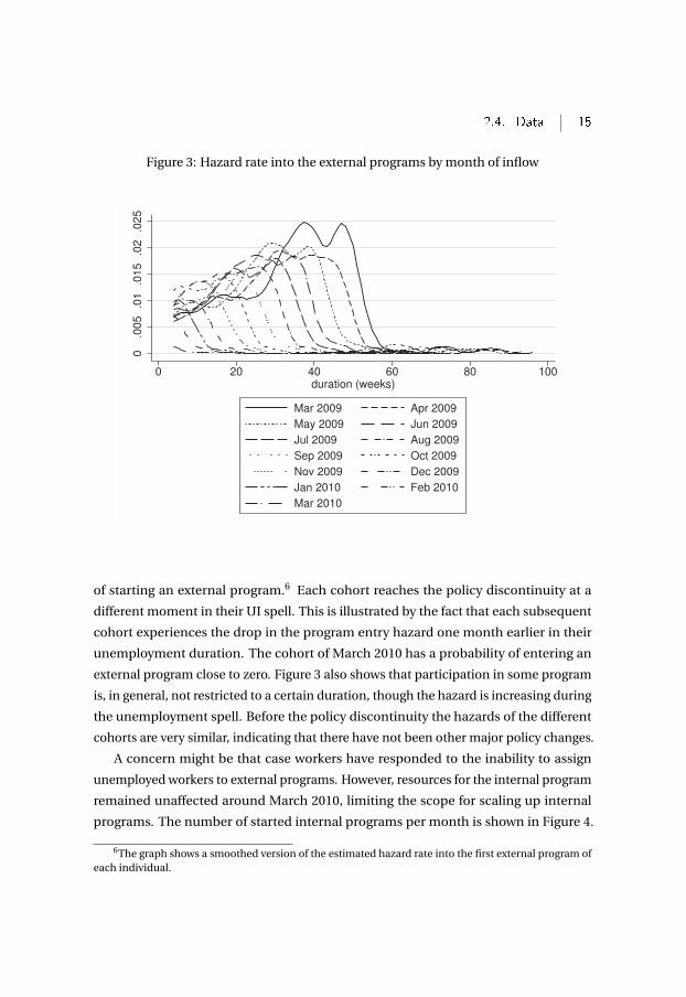
Figure 3: Hazard rate into the external programs by month of inflow
0.0
05
.01
.015
.02
.025
0 20 40 60 80 100duration (weeks)
Mar 2009 Apr 2009
May 2009 Jun 2009
Jul 2009 Aug 2009
Sep 2009 Oct 2009
Nov 2009 Dec 2009
Jan 2010 Feb 2010
Mar 2010
of starting an external program.6 Each cohort reaches the policy discontinuity at a
different moment in their UI spell. This is illustrated by the fact that each subsequent
cohort experiences the drop in the program entry hazard one month earlier in their
unemployment duration. The cohort of March 2010 has a probability of entering an
external program close to zero. Figure 3 also shows that participation in some program
is, in general, not restricted to a certain duration, though the hazard is increasing during
the unemployment spell. Before the policy discontinuity the hazards of the different
cohorts are very similar, indicating that there have not been other major policy changes.
A concern might be that case workers have responded to the inability to assign
unemployed workers to external programs. However, resources for the internal program
remained unaffected around March 2010, limiting the scope for scaling up internal
programs. The number of started internal programs per month is shown in Figure 4.
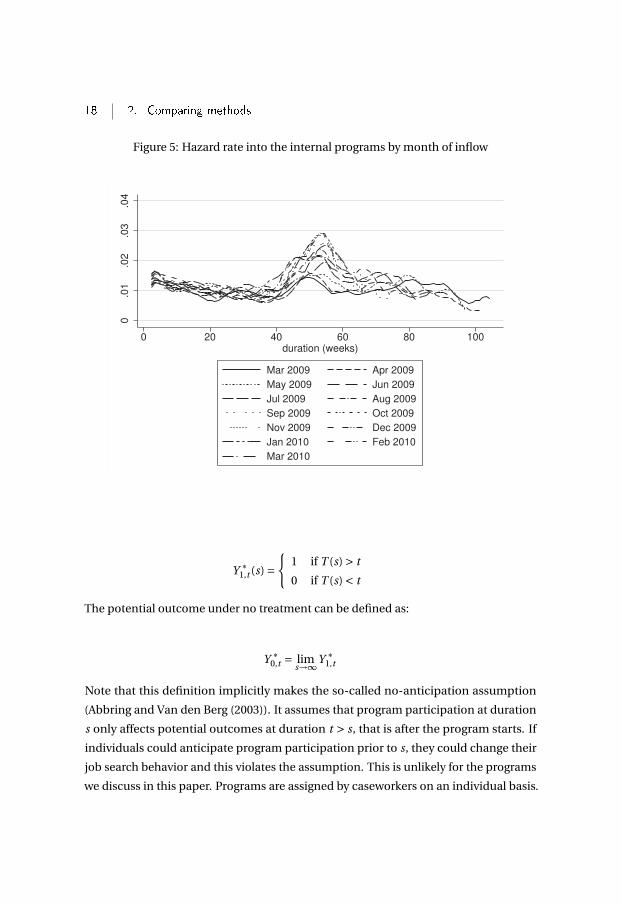
6The graph shows a smoothed version of the estimated hazard rate into the first external program ofeach individual.

16 2. Comparing methods
Internal programs are only recorded from 2009 onward. The policy discontinuity of
March 2010 is indicated by the dashed line. There is no indication of a response around
the date of the policy discontinuity. Separate graphs by type of program are provided
in the appendix of Muller et al. (2015). The hazard rates into an internal program for
different cohorts are shown in Figure 5. The hazard rates are very similar, supporting
the assumption that internal program provision was unaffected by the policy change.7
A further concern might be that even though the number of internal programs was
not changed, case workers may have reacted to the unavailability of external programs
by shifting their internal programs to these individuals that might otherwise have
participated in external programs. This would imply that the policy does not change
external program participation to no participation, but, for some individuals, changes
it to internal program participation.
To investigate whether such a shift of internal program targeting indeed occurred,
we present mean values of characteristics of individuals enrolling in an internal program
per month in Figure 6. Mean age and weekly hours of unemployment are shown in
panel (a) of Figure 6, unemployment and disability history and education level are
shown in panel (b), the previous hourly wage is shown in panel (c) and the share of
nine industry categories is shown in panel (d). None of the graphs indicate any kind
of discontinuity around March 2010. This suggests that case workers did not shift
internal programs to individuals who would otherwise enroll in an external program.
The effect of enrollment in an external program should thus be interpreted as the effect
conditional on the allocation of internal programs.
2.5 Treatment e�ects
In this section we define the relevant treatment effects and discuss how they are
identified from the policy discontinuity.
2.5.1 De�ning the treatment e�ect
Recall that only a small share of all unemployed workers enters an external program
during their unemployment spell. Due to the selectivity of treatment participation,
7In theory, job seekers could decide to pay for an external program themselves once it is no longeroffered through the UI administration. However, the costs of these programs are considerable, especiallyfor unemployed, such that this never happens in the Netherlands.

2.5. Treatment e�ects 17
Figure 4: Distribution of starting dates of the internally provided programs0
1000
2000
3000
Num
ber
of p
rogr
am s
tart
s
2009m1 2009m7 2010m1 2010m7 2011m1Starting month program
the composition of the program participants differs from the non-participants. We are
interested in the treatment effect for this specific subsample. Therefore we focus on the
average treatment effect on the treated (ATET), which is defined in the literature as the
mean difference between potential outcomes under treatment and non-treatment, for
those that receive treatment (see for example Heckman et al. (1999)).
Our key outcome of interest is duration until employment, which is a random
variable denoted by T > 0. Define Yt =1(T > t ), a variable equal to one if the individual
is still unemployed in period t , and zero otherwise. Define S to be a random variable
denoting the duration at which program participation starts (with realized value s).
Potential unemployment duration depends on program participation. The dynamic
nature of duration data implies that even for a single program many different treatment
effects arise. The program can start at different durations, while the effect can be
measured at different points in time (see for an extensive discussion of dynamic
treatment effects Abbring and Heckman (2007)). We can define potential outcomes
when treated as:
18 2. Comparing methods
Figure 5: Hazard rate into the internal programs by month of inflow
0.0
1.0
2.0
3.0
4
0 20 40 60 80 100duration (weeks)
Mar 2009 Apr 2009
May 2009 Jun 2009
Jul 2009 Aug 2009
Sep 2009 Oct 2009
Nov 2009 Dec 2009
Jan 2010 Feb 2010
Mar 2010
Y ∗1,t (s) =
{1 if T (s) > t
0 if T (s) < t
The potential outcome under no treatment can be defined as:
Y ∗0,t = lim
s→∞Y ∗1,t
Note that this definition implicitly makes the so-called no-anticipation assumption
(Abbring and Van den Berg (2003)). It assumes that program participation at duration
s only affects potential outcomes at duration t > s, that is after the program starts. If
individuals could anticipate program participation prior to s, they could change their
job search behavior and this violates the assumption. This is unlikely for the programs
we discuss in this paper. Programs are assigned by caseworkers on an individual basis.

2.5. Treatment e�ects 19
Figure 6: Composition of the internal program participants
(a) Mean of age and hours unemployed bymonth
3540
4550
2009m4 2009m10 2010m4 2010m10
Age Weekly hours of unemployment
(b) Mean of characteristics by month
0.1
.2.3
.4
2009m4 2009m10 2010m4 2010m10
# of unempl. spells previous 3 years % low educated% high educated % disabled or sickness
(c) Mean of hourly wage by month
1919
.219
.419
.619
.8
2009m4 2009m10 2010m4 2010m10
Hourly wage previous employment
(d) Mean of industry shares by month
0.1
.2.3
2009m4 2009m10 2010m4 2010m10
There are no strict criteria for participation and each period only a small fraction of the
unemployed workers can enroll, so it is impossible for job seekers to know in advance
when they will enter the program. In the remainder of the paper we assume that the
no-anticipation assumption holds.
Individuals leave unemployment after different durations, such that the compo-
sition of the survivors changes over time. This issue, known as dynamic selection,
necessitates defining the subgroup for which the treatment effect is defined (see Van den
Berg et al. (2014)). First, we are interested in the average treatment effect on individuals
that received treatment, such that we condition on S = s. Second, the effect is defined
on individuals that survived up to duration s, such that we also condition on T > s. This
effect is defined by Van den Berg et al. (2014) as the average treatment effect on the

20 2. Comparing methods
treated survivors at time t (AT T S(s, t )), with as arguments the timing of treatment and
the time at which the outcome is measured.
AT T S(s, t |S = s) = E[
Y ∗1,t (s)−Y ∗
0,t
∣∣∣T > s,S = s]
(2.1)
This is the treatment effect that we will focus on in the analysis.
2.5.2 Identi�cation
Estimating the ATTS (equation (2.1)) without making parametric assumptions is
generally not possible from observational data (Abbring and Van den Berg (2005)).
A policy discontinuity provides exogenous variation which may allow to estimate the
ATTS (Van den Berg et al. (2014). Consider two cohorts of entrants in unemployment.
The first enters unemployment at some point in time, with the time until the policy
change equal to t1. The second cohort enters unemployment later, but still before the
policy change. For this cohort the time until the policy change equals t2 < t1. This
is illustrated in Figure 7. The two cohorts face the same policy of potential program
assignment for t2 time periods, implying that dynamic selection is the same up to this
point. After t2, the first cohort faces another period of potential program assignment,
with length t1 − t2, while the second cohort is excluded from program participation.
As a result, we can compare the outflow to employment in the two cohorts, for those
individuals that survived up to t2 and did not enroll in a program prior to t2.
To assign differences in job finding between these groups to program participation,
two assumptions should hold. First, the policy discontinuity should be unanticipated
by unemployed workers and case workers. Anticipation of the policy discontinuity is
problematic, as behavior of job seekers or case workers may be affected in the period just
before March 2010. The policy change we are investigating however has the advantage
that it was unexpected. The UI administration only realized late that there was no
longer budget for these programs and expected that the Ministry of Social Affairs would
extend the budget. Enrollment in the external programs stopped immediately after
an extension of the budget was rejected. Since not even the UI administration was
expecting the change, we can safely assume that job seekers and case workers did
not anticipate it either. The second assumption is that there should be no differences
between the two cohorts in factors that affect job finding, other than the difference in
program assignment. We discuss this assumption below.

2.5. Treatment e�ects 21
Figure 7: Treatment effect identification
t2
t1
Cohort 1
Cohort 2
Policydiscontinuity
(Calendar) time}t1 − t2
2.5.3 Business cycle, seasonalities and cohort composition
Even if two cohorts are compared that enter unemployment relatively shortly after each
other, changes in the labor market conditions may lead to differences in outcomes. We
discuss how this may affect our estimates, and how we correct for this. Figure 8 presents
the unemployment rate and the inflow and outflow of unemployment. The two vertical
full lines indicate the observation period that is used in the analysis. The vertical dashed
line indicates the policy discontinuity. In the period before the policy discontinuity,
2009 and the beginning of 2010, unemployment was rising. During 2010 it decreased
slightly, while in 2011 it started increasing again. In the short-run, seasonalities are the
main source of fluctuations in unemployment. Also inflow into and outflow from UI are
relatively stable around the policy discontinuity, except for short-run fluctuations. Such
fluctuations in labor market conditions may affect outcomes in two ways. First, they
affect the composition of the inflow into unemployment. For example, the financial
crisis may cause that different types of workers become unemployed. A changing
composition may also affect aggregate outflow probabilities. Second, labor market
conditions affect outflow probabilities directly, as it is often more difficult to find
employment when unemployment is high.
To correct for differences in composition we exploit the set of covariates in the
data. In particular, we use weights to make each cohort in composition of observed
characteristics comparable to the March 2010 cohort. As characteristics we use three
previous hourly wage categories, an indicator for having been unemployed in the past

22 2. Comparing methods
Figure 8: Labor market indicators
01
02
03
04
05
06
07
08
0F
low
s (
x 1
00
0)
01
23
45
67
Un
em
plo
ym
en
t (%
)
2008m1 2009m1 2010m1 2011m1 2012m1 2013m1
Unemployment Unemployment seasonally adj.
Inflow UI Outflow UI
Source: Centraal Bureau voor de Statistiek (CBS), Statline.
three years, an indicator for being married or cohabiting, age categories, an indicator
for being part-time unemployed (less than 34 hours per week)8 and three education
categories. Interacting these covariates we obtain 288 groups. Define the share of group
g in cohort c by αc,g . The weight assigned to an observation belonging to group g in
cohort c is defined by:
wc,g = αmar 2010,g
αc,g
We define the survivor functions that will be estimated in the analysis, as the weighted
average of the survivor functions of each cohort-group:
Fc (t ) =∑g
wc,g Fc,g (2.2)
However, the results are robust against using weights.
The direct effect of the business cycle and seasonal effects on employment probabil-
ities requires some more discussion. To formalize these factors, consider the following
8Since this is based on the previous job, it captures the part-time and full-time employment.

2.5. Treatment e�ects 23
simple model. Assume that the hazard rate to employment (h) for cohort c depends
on the duration of unemployment (t), the effect of the business cycle (bc ), the effect
of seasonalities (lc ) and the effect of entry into a program at time s, which is γ(s). To
correct for business cycle effects when identifying the effect of program participation,
we need to make some assumptions about the hazard. We assume that the business
cycle, seasonalities and treatment have an additive effect on the baseline hazard, where
each of these impacts may vary by unemployment duration t . Note that this is very
flexible as we do not assume anything on how these factors vary by duration. The
duration dependence of the hazard is denoted by λ(t ), which is common for all cohorts.
The hazard rate is given by
h(t , s,c) =λ(t )+bc (t )+ lc (t )+γ(s, t ) (2.3)
From the hazard rate we can construct the survival function.
Fc (t ) = exp(−∫ t
0h(u)du
)= exp
(−∫ t
0λ(u)du −
∫ t
0bc (u)du −
∫ t
0lc (u)du −
∫ t
sγ(u)du
)Taking the logarithm of the survival function we have:
log Fc (t ) = −∫ t
0λ(u)du −
∫ t
0bc (u)du −
∫ t
0lc (u)du −
∫ t
sγ(u)du
≡ ∆(t )+Bc (t )+Lc (t )+Γ(s, t )
This implies that the business cycle, seasonalities and program participation have
additive impacts on the log of the survival function. Seasonalities are by definition
those factors that are common across different years, such that Lc (t ) = Lc−12(t ), for all c .
The difference in log survivor functions of two cohorts identifies the treatment effect
plus the difference in seasonal and business cycle effects. For example, comparing the
January 2010 cohort with the October 2009 cohort we get:
µ1(t ) = log F j an10(t )− log Foct09(t )
= Γ(s, t )+ [L j an10(t )−Loct09(t )
]+ [B j an10(t )−Boct09(t )
](2.4)
If we condition both survivor functions on survival up to t2 (in this case t2 = two months),
the January 2010 cohort never enters a program, while a share of the October 2009 cohort
enters a program. The term Γ(s, t) measures the effect of program participation of a

24 2. Comparing methods
share of a cohort, and can thus be interpreted as an intention-to-treat effect. Below
we discuss how to this relates to the ATTS (equation 2.1). The size of the bias due
to the remaining terms, (L j an10(t)−Loct09(t)) and (B j an10(t)−Boct09(t)), depends on
the length of the time interval between the two cohorts, and the volatility of the labor
market.
We can possibly improve on this estimator by applying an approach somewhat
related to a difference-in-differences estimator. By subtracting the same cohort
difference from a year earlier, we eliminate the seasonal effects, at the cost of adding
extra business cycle effects:
µ2(t ) = [log F j an10(t )− log Foct09(t )
]− [log F j an09(t )− log Foct08(t )
]= Γ(t )+
[B j an10(t )−Boct09(t )
]+
[B j an09(t )−Boct08(t )
](2.5)
Whether this is preferable over µ1(t) depends on the relative sizes of the business
cycle and seasonal effects. Figure 8 suggests that, if the interval is sufficiently small,
seasonal effects are larger than business cycle effects. Given a small interval such as
three months, business cycle effects may be small enough to ignore, such that µ2 is a
satisfactory estimator of Γ(t ). Note that this estimator is an extension of the approach
suggested by Van den Berg et al. (2014). They propose exploiting a policy discontinuity
to estimate effects on a duration variable. We add to this approach by taking double
differences.
The estimators µ1(t) and µ2(t) estimate intention-to-treat effects, since not all
unemployed workers in the earlier cohort enter a program. The average treatment
effect on the treated survivors follows from dividing the intention to treat effect by the
difference in the share of each cohorts that enrolls in the program. Define F tr eat as
the survivor function for treatment, where an exit is defined to be the start of the first
program. The ATTS estimator is given by:
àAT T S(t2, t ) = µ1(t )
log F Tr eatj an10(t )− log F Tr eat
oct09 (t )(2.6)
And similar for µ2(t ).
2.6 Quasi-experimental analysis
We start by defining which cohorts to compare. A cohort contains all individuals
entering unemployment within one particular month. The time interval between

2.6. Quasi-experimental analysis 25
cohorts should be small to minimize business cycle and seasonal effects, but the trade-
off is that more time between cohorts increases the difference in exposure to potential
program participation. We use cohorts three months apart. Second, to exploit the policy
discontinuity, the cohorts should not enter unemployment too long before March
2010. Therefore, we use the cohorts of October 2009 until January 2010, facing between
five and two months of potential program participation, respectively. Each cohort
will be compared to the cohort entering unemployment three months earlier. The
survivor function of each cohort is presented in Figure 9. Around 50% of the UI benefits
recipients find work within 12 months, while after two years around 65% has found
work.
2.6.1 Intention-to-treat e�ect
We first take the difference between the log of the survivor function and the log of the
survivor function of the cohort entering unemployment three months earlier (µ1(t )).9
This compares the outflow of a cohort from in which no one enrolls in the program to
outflow of a cohort in which a share enrolls in the program. As discussed in subsection
2.5.2, we condition on survival and no-treatment up to the duration at which the
later cohort reaches the policy discontinuity. So when comparing January 2010 with
October 2009, only individuals are included with an unemployment duration of at least
three months and who do not start an external program in the first two months. The
differences up to a duration of 18 months after inflow in unemployment are presented
in panel (a) of Figure 10.10 We find a negative effect on job finding during the first few
months after program participation of around 4%-points in three of the four estimates.
After about 10-12 months the negative effect disappears and all estimates are close to
zero.
These estimates are based on simple differences between cohorts, thus not taking
fluctuations in labor market conditions into account. By subtracting the same differ-
ences from a year earlier, we correct for cohort differences that are constant across years
(such as seasonalities). Estimates from such a “difference-in-differences” approach
9All estimates presented in this section are estimated using weights as discussed in subsection 2.5.3.10For the ease of interpretation, in the graph we present a transformation of the estimates µ1. We
display [exp(µ1)−1]F ], which is the effect on the actual survival function. So the graph can be interpretedas the effect on the probability of finding employment. The same transformation is made in subsequentgraphs.

26 2. Comparing methods
Figure 9: Survivor functions by month of inflow
.2.4
.6.8
1
Surv
ivor
Function
0 10 20 30
Time
Jan 2010 Dec 2009
Nov 2009 Oct 2009
Figure 10: Intention-to-treat effect estimates, conditional on T > t2,S > t2
(a) µ1(t )
−.0
8−
.04
0.0
4.0
8E
ffect
on
surv
ival
func
tion
0 5 10 15 20Time
Jan 2010−Oct 2009 Dec 2009−Sep 2009Nov 2009−Aug 2009 Oct 2009−Jul 2009
(b) µ2(t )
−.0
8−
.04
0.0
4.0
8E
ffect
on
surv
ival
func
tion
0 5 10 15 20Time
Jan 2010−Oct 2009 Dec 2009−Sep 2009Nov 2009−Aug 2009 Oct 2009−Jul 2009
(µ2(t )) are presented in panel (b) of Figure 10.11 Again we find a negative effect on job
finding in the first months. At longer durations, the estimates diverge somewhat. In the
appendix of Muller et al. (2015) each line is presented with a 95% confidence interval
(standard errors are computed using bootstrapping). The early negative effect is always
significantly different from zero, while none of the estimates at longer durations are
11When estimating µ2(t) we only present estimates up to the duration at which the cohorts froma year earlier reach the policy discontinuity, which is between 15 and 18 months. Estimates at longerdurations are biased as the earlier cohorts are affected by the policy discontinuity as well.

2.6. Quasi-experimental analysis 27
significantly different from zero. Note that each comparison measures the effect of
additional treatment at a slightly different duration. For example, the January 2010-
October 2009 comparison measures the effect of additional treatment in the 4th-6th
month of unemployment, while the December 2009-September 2009 comparison
measures the effect of additional treatment in the 5th-7th month of unemployment.
The results show a pattern that is quite consistent across different cohort com-
parisons and across the two estimators. Job finding is significantly reduced in the
early months, while the difference disappears after 6-12 months. This finding is in
line with the lock-in effect often found in the literature (see for example Lechner and
Wunsch (2009)). The lock-in effect implies that when a program starts, participants
shift attention from job search to the program which reduces their job finding rate. This
negative effect disappears after some months, but we do not find any (positive) effects
at longer durations.
2.6.2 Average treatment e�ect
The above findings are intention-to-treat effects. To estimate the average effect of
treatment on individual employment probabilities they need to be scaled by the
differences in treatment intensity. We divide each estimate by the difference in program
participation of the cohorts that are being compared (as defined in equation (2.6)).
The difference in program participation occurs during a three months period in which
the later cohort reached the policy discontinuity but the earlier cohort did not. We
estimate the difference in program participation by the difference between the survivor
functions for program participation (as defined in subsection 2.5.3). For example, when
comparing the January 2010 cohort with the October 2009 cohort, the difference in
program participation is given by
F tr eatJan10(t |T,S > 2 months)− F tr eat
Oct09(t |T,S > 2 months) (2.7)
And similar for the other cohorts that are compared. These estimates are presented
in panel (a) of Figure 11. We find a clear increase as soon as the first cohort reaches
March 2010. The difference increases for approximately three months, after which the
comparison cohort reaches March 2010. From that point onward, both cohorts receive
no treatment, and the difference remains stable. The difference is between 15 and 20%-
points. The difference in program participation can also be computed using the same

28 2. Comparing methods
Figure 11: Differences in program participation, conditional on T > t2 and S > t2
(a) Simple difference
−.4
−.3
−.2
−.1
0.1
.2.3
.4E
ffect
on
surv
ival
func
tion
(pro
gram
)
0 5 10 15 20Time
Jan 2010−Oct 2009 Dec 2009−Sep 2009Nov 2009−Aug 2009 Oct 2009−Jul 2009
(b) Double difference
−.4
−.3
−.2
−.1
0.1
.2.3
.4E
ffect
on
surv
ival
func
tion
(pro
gram
)
0 5 10 15 20Time
Jan 2010−Oct 2009 Dec 2009−Sep 2009Nov 2009−Aug 2009 Oct 2009−Jul 2009
“difference-in-differences” approach as in µ2(t ). Such estimates are presented in panel
(b) of Figure 11. Due to differencing with cohorts from a year earlier, the differences are
less smooth, though the main pattern remains. Confidence intervals are presented in
the appendix of Muller et al. (2015). All differences are highly significant.
The results of dividing the estimates from panel (a) in Figure 10 by the treatment
difference are presented in panel (a) of Figure 12. The pattern does not differ much from
that of the intention-to-treat effects. Program participation reduces the job finding
probability during the first two-three months by about 40%-point, while after ten
months employment probabilities are similar again and there is no significant effect.
The double differencing estimates (µ2(t )) are presented in panel (b) of Figure 12. The
pattern is quite similar. There is a negative effect on the job finding probability of 40%-
point directly after program participation starts, which decreases in magnitude over
time towards a zero effect after about eight months (confidence interval are presented
in the appendix of Muller et al. (2015)).
Since the policy discontinuity reduced program participation to zero, these es-
timates can be interpreted as average treatment effects on the treated, rather than
local average treatment effects. Alternatively, if the policy discontinuity only had
reduced program participation (but not to zero), our approach would have estimated
the treatment effect on those individuals that would have participated before the policy
discontinuity but not afterwards. In the terminology of instrumental variables, these are
the “compliers”. The fact that the policy discontinuity reduced program participation to
zero, implies that there are no “always-takers”, and the local average treatment effect
equals the average treatment effect.

2.6. Quasi-experimental analysis 29
Figure 12: Average treatment effect, conditioned on T > t2,S > t2
(a) based on µ1(t )
−.8
−.6
−.4
−.2
0.2
.4.6
.8E
ffect
on
surv
ival
func
tion
0 5 10 15 20Time
Jan 2010−Oct 2009 Dec 2009−Sep 2009Nov 2009−Aug 2009 Oct 2009−Jul 2009
(b) based on µ2(t )
−.8
−.6
−.4
−.2
0.2
.4.6
.8E
ffect
on
surv
ival
func
tion
0 5 10 15 20Time
Jan 2010−Oct 2009 Dec 2009−Sep 2009Nov 2009−Aug 2009 Oct 2009−Jul 2009
2.6.3 Common trend assumption
The assumption that the business cycle terms in (2.5) are negligible has some similarities
with the common trend assumption in a difference-in-differences estimator. It requires
that in the absence of the policy discontinuity, the difference in employment rate
between the January and November cohort would have been the same in 2009/2010
as a year earlier in 2009/2008. This is by definition untestable. However, we can get an
indication of the plausibility of the assumption, by investigating the survivor functions
over the first months of each cohort, so before exposure to the policy discontinuity. All
estimators condition on survival up to t2, but we can use information on job finding
before t2 to get some indication about the validity of our common trend assumption.
To have a sufficient number of pre-discontinuity months in the latest cohort, we focus
on the comparisons of December 2009, November 2009 and October 2009. Basically, we
estimate µ2(t ) for t ≤ t2, without conditioning on survival up to a certain duration.
Estimates are presented in Figure 13 for December 2009 - September 2009, Novem-
ber 2009 - August 2009 and October 2009 - July 2009, including 95% confidence intervals,
computed using bootstrapping. We find that all estimates are significantly negative,
though small in magnitude. This implies that the treatment effect estimates are biased
downwards somewhat, and thus provide lower bounds of the effect. Obviously our
approach does not fully control for business cycle variation in job finding rates.

30 2. Comparing methods
Figure 13: Common trend tests, µ2(t ), three months differences
(a) December 2009 - September2009
−.1
5−
.1−
.05
0.0
5.1
.15
1 2 3 4
Time
(b) November 2009 - August2009
−.1
5−
.1−
.05
0.0
5.1
.15
1 1.5 2 2.5 3
Time
(c) October 2009 - July 2009
−.1
5−
.1−
.05
0.0
5.1
.15
1 1.2 1.4 1.6 1.8 2
Time
2.7 Non-experimental analysis
The administrative dataset contains a rich set of covariates. In this section we investigate
whether the quasi-experimental estimates from the previous section can be reproduced
when, instead of exploiting the policy discontinuity, we correct for observable differ-
ences between treated and non-treated individuals. We apply a matching estimator in
subsection 2.7.1 and estimate the timing-of-events model in subsection 2.7.2.
2.7.1 Matching
Matching methods typically denote a set of estimators to compute counterfactual out-
comes in the absence of randomized assignment to treatment (Imbens and Wooldridge
(2009), Abadie and Imbens (2011)) and date back to Rosenbaum and Rubin (1983).
The approach relies on two main assumptions. First, selection into treatment is on
observables only:
Y ∗0,t (s),Y ∗
1,t (s) ⊥ S|X (2.8)
Also referred to as the unconfoundedness assumption, it implies that after conditioning
on a set of observed characteristics, assignment to treatment is independent of the
potential outcomes. If selection into treatment is on observable characteristics only, a
counterfactual outcome can be constructed using different methods that correct for
the differences in observed characteristics. Matching is closely related to a simple OLS
framework which can also correct for differences in observable characteristics and
relies on a similar unconfoundedness condition. However, in an OLS regression this
assumption is combined with strong functional form assumptions (covariates enter the

2.7. Non-experimental analysis 31
model additively and linearly), such that the model is much more restrictive (Imbens
(2014)).
If treatment selection occurs also on non-observables, matching estimators yield
biased results. The bias of matching estimators depends on the degree of selection that
is captured by observed characteristics. Including a rich set of covariates is thus crucial.
It is often argued that employment histories are particularly important, because they
are strong predictors of future labor market outcomes as well as program participation
(see, for example, Card and Sullivan (1988), Heckman et al. (1999), Gerfin and Lechner
(2002), Lechner et al. (2011)). Our administrative data set allows the use of a rich set of
covariates. We include individual characteristics (age, education level, marital status,
region), employment history variables (previous hourly wage, unemployment history,
previous industry) and current unemployment spell variables (unemployment size in
hours, a sickness or disability dummy, maximum UI eligibility). We thus include a set
of covariates that is as rich as usually available in evaluations of active labor market
programs. Still, excluding that selection also depends on unobserved characteristics
remains a strong assumption.
The second condition for applying matching is that there is a common support in
the distribution of the covariates between program participants and non-participants.
The common support assumption states:
0 < Pr(S <∞|X = x) < 1 ∀x
It implies that, in order to match program participants with non-participants who
are similar with respect to covariates, a complete overlap in the distribution of these
covariates is required between the two groups. A way of investigating whether this
assumption is likely to hold is to estimate a propensity score model and plot the density
of predicted values for treated and non-treated individuals. The overlap assumption
is likely to be violated in case there is little overlap in the two densities, or if there is
a lot of mass close to zero or one in one of the groups (Busso et al. (2009)). In the
appendix of Muller et al. (2015) the predicted propensity scores for treated and non-
treated individuals are presented, after estimating a logit model for the likelihood of
being treated. The plot suggests that there is sufficient overlap: both densities have
most mass between 0.05 and 0.3 and there is hardly any mass close to zero or one.
Furthermore, there are no (combinations of) individual characteristics that perfectly
predict program participation.
32 2. Comparing methods
The matching approach implies that we use variation in program participation
within a particular cohort, as opposed to comparing different cohorts. We start by
defining the treatment and the cohorts we use in the analysis. The sample should
overlap with that used in the previous section, such that the distribution of individual
characteristics and labor market conditions are the same. Therefore, we include
individuals entering unemployment between October 2009 and January 2010, which
are the same cohorts used for the quasi-experimental estimates. In order to estimate
the same treatment effect as in our non-experimental analysis, we define treatment as
being selected for program participation between three and five months and exclude all
individual that leave unemployment before three months or those that start a program
before three month. This makes again a no-anticipation assumption (as discussed
in Section 2.5). This corresponds to the effect that we measure in the January 2010 -
October 2009 comparison in Figure 12. All other individuals are classified as belonging
to the control group, however we censor their observation if they start a program after
five months. In the next section we provide the details of this approach, which is similar
to that used by Lalive et al. (2008). From the perspective of assessing the performance
of the matching approach, the estimates should not be based on a sample in which
treatment assignment is affected by the policy discontinuity. The sample that we use
might be slightly affected. The impact on the estimates should be small though, because
we censor all control group observations when they start a program. As a robustness
check we show that using a sample consisting of the same monthly cohorts from 2008
instead of 2009 gives very similar estimates.
Standard static matching estimators require excluding individuals who start treat-
ment after five months from the pool of potential controls. If they would be included,
it would change the interpretation of the estimate into the effect of early treatment
relative to later treatment, which is not the parameter we are interested in (e.g. Sianesi
(2004)). Excluding these observations is problematic as well, as it creates a selective
control group. To address this problem we take the following approach. First, we use a
logistic model to predict for each individuals the propensity score, classifying those that
start treatment in three to five months as the treated group, and all others as the control
group.12
Next, we estimate for both the treated and the matched control group the Kaplan-
Meier survival functions, using as weights the inverse of the predicted propensity
12All individuals leaving unemployment before three months or starting treatment before threemonths are excluded, which was also done in the quasi-experimental approach.

2.7. Non-experimental analysis 33
Figure 14: Average treatment effect on the treated (with 95% confidence intervals):Matching estimator using Kaplan-Meier survival functions
(a) Oct 2009 - Jan 2010
−.5
−.4
−.3
−.2
−.1
0.1
.2.3
.4.5
0 5 10 15 20
Months
(b) Oct 2008 - Jan 2009
−.5
−.4
−.3
−.2
−.1
0.1
.2.3
.4.5
0 5 10 15 20
Months
scores.13 All control group observations that start treatment after five months are
censored at the start of their program. This way, we include all potential control
observations, avoiding bias due to dynamic selection. The difference between the
survival functions provides an estimate of the average treatment effect on the treated.
Standard errors are again computed using bootstrapping. The estimates, including
a 95% confidence interval are presented in panel (a) of Figure 14. The estimates of
the effect of program participation on the job finding probability are significantly
negative at any duration, though the negative effect becomes smaller over time. At an
unemployment duration of five months, those that started treatment during three-to-
five months have an almost 20%-points lower probability of having found employment.
This difference decreases to 10%-points after 18 months of unemployment.
As an alternative, we use a dataset including individuals entering unemployment
one year earlier. Those are unaffected by the policy discontinuity, however they may
face different labor market conditions. Estimates are presented in panel (b) of Figure
14. The results are very similar, showing the same negative effect which decreases in
magnitude over time. Standard errors are slightly larger, which is due to the fact that
more control group individuals enter the program after five months and have to be
censored at that point.
13For control group individuals the weights are given by p(Xi ), the predicted probability of beingtreated. For treated individuals the weights are given by 1− p(Xi ).

34 2. Comparing methods
We conclude that the estimates are quite robust to the choice of the sample. Each
shows a negative estimate of the program effect, which is almost 20%-points after
five months of unemployment, and decreases in magnitude to a negative effect of
5-10%-points after 18 months of unemployment.
2.7.2 Timing of events model
Matching requires little functional form assumptions, but relies the on the conditional
independence assumption (defined in (2.8)). The timing-of-events model (Abbring and
Van den Berg (2003)) relaxes the conditional independence assumption, at the cost of
imposing stronger functional form assumptions. It has become popular in the literature
on dynamic treatment evaluation (see for example Abbring et al. (2005), Van den Berg
et al. (2004), Lalive et al. (2005) and Van der Klaauw and Van Ours (2013)). In this
subsection we estimate this model to assess whether it can reproduce the findings from
the quasi-experimental approach.
The timing-of-events model specifies jointly job finding and entry in the program
using continuous-time duration models. To control for unobserved characteristics
the unobserved heterogeneity terms in both hazard rates are allowed to be correlated.
Identification relies on a mixed proportional structure of both hazard rates. Like both
earlier approaches (quasi-experimental and matching) also the timing-of-events model
makes the no-anticipation assumption. Note that it does not rule out that the treatment
probability differs between individuals and that individuals are aware of this. Some job
seekers may have a high probability of program assignment and know this. Only the
exact timing of the program start should be unanticipated.
Consider an individual entering unemployment at calendar date τ. Her baseline job
finding rate depends on the number of days of unemployment (t) and is denoted by
we (t). Calendar time fixed effects are captured by the function qe (τ0 + t ). The hazard
rate further depends on observed characteristics (x) and unobserved characteristics ve .
After starting a program, the hazard rate is shifted by the treatment effect δ. Since the
treatment is likely to affect the hazard differently over duration, we include a flexible
specification with a set of effects, δn It∈(sn ,sn+1). For values of t between sn and sn+1,
the indicator function It∈(sn ,sn+1) equals one. The effect of program participation starts

2.7. Non-experimental analysis 35
directly after the start of the program (s1 = s). We allow different effects for the first six
months (s2 = 6) and the period after six months. The job finding hazard rate is given by:
he (t |x,τ0, s, vT ) = we (t )qe (τ0 + t )exp[
xβe +N∑nδn It∈(sn ,sn+1)
]ve (2.9)
Estimation of equation (2.9) yields a biased estimate of the treatment effects if program
participation is (even conditional on the observed characteristics) non-random. In
that case program participation is correlated with the unobserved determinants of
unemployment duration ve . To account for this, program participation is modeled
jointly, also using a mixed proportional hazard rate:
ha(t |x,τ0, va) = wa(t )qa(τ0 + t )exp(xβa)va (2.10)
With all notation similar to equation (2.9). The unobserved term va is allowed to be
correlated with ve , with joint discrete distribution g (ve , va). We take g (ve , va) to be a
bivariate discrete distribution with an unrestricted number of mass points indexed by
k. The corresponding probabilities are:
pk = P (ve = vke , va = vk
a ) ∀k
Estimation results show that using k = 2 is already sufficiently flexible. Increasing
the number mass points leads to zero probability for these excess mass points. We
parameterize the duration dependence pattern of the hazards (wT (t), wS(s)) with a
piecewise constant function:
w j (t ) =M∑
m=1πm Itm−1≤t<tm
Where Itm−1≤t<tm is an indicator for duration being between tm−1 and tm and πm the
function value. This function is very flexible, as by increasing the number of intervals
m it can approximate any pattern arbitrarily well. We use the following intervals (in
months): 0-2, 2-4, 4-6, 6-9, 9-12, 12-18, 18-24, 24-48.
Calendar time effects are also modeled by a piecewise constant function, where each
interval is taken to be a quarter-of-a-year.14 Estimation of the parameters is performed
by maximizing the log-likelihood, in which right-censoring is straightforwardly taken
into account. The model is estimated using the full dataset of 116,866 observations.
14We normalize the function value for the first interval to one in each of the four piecewise constantfunctions.

36 2. Comparing methods
Table 2: Treatment effect estimates Timing-of-Events model
Coefficient p-valueδ(0−2 months) -0.42 0.00δ(3−6 months) -0.12 0.00δ(≥6 months) 0.05 0.00
The estimates of the treatment effects are presented in Table 2.15 The effect of
program participation is estimated to have a large, significantly negative effect on
the job finding rate in the first two months (δ0−2 months), with the coefficient equal
to -0.42. In the third and fourth month the effect is still significantly negative, but
smaller in magnitude (-0.12). After six months (δ≥6 months) program participation has
a small, significantly positive effect on the probability of finding a job. To interpret
the magnitude of these effects, we transform them into an effect on the probability
of being employed at some duration t since being unemployed. This can be done by
computing the survivor function for an average individual (we take the mean value of
each individual characteristic in the sample), entering unemployment in December
2009. We simulate the survivor based on the estimated model twice. Once imposing
that the individual never participates in a program, the second time imposing program
participation after two months of unemployment. Both survivor functions (up to a
duration of two years) are presented in panel (a) of Figure 15, including one standard
error bounds. Standard errors are computed using the delta method. Participating
in a program after two months of unemployment lowers the probability of being
employed subsequently, in accordance with the negative effect estimate. The difference
between the survivors is presented in panel (b) of Figure 15. The effect is significantly
negative directly after the program starts, and increases in magnitude up to a 5%-
points difference after six months. Afterwards the effect decreases in magnitude and as
standard errors increase it is no longer significantly different from zero after about 14
months.
15Full estimation results are presented in the appendix of Muller et al. (2015). Most covariates havethe expected sign and are highly significant. The oldest age group has a lower job finding rate, as do lowereducated individuals. Being (partially) disabled, sick or having an unemployment history also reducesthe job finding rate. Furthermore we find that the job finding rate decreases steadily over unemploymentduration. As expected there are some fluctuations in the job finding rate related to the calendar time. Incolumn (3) the coefficients of the treatment hazard are presented (equation (2.10)).

2.8. Discussion 37
Figure 15: Timing-of-events model: Simulated treatment effect
(a) Simulated survivor functions (with one stan-dard error bounds)
.2.4
.6.8
1S
urv
ival fu
nction
0 200 400 600Time (days)
Untreated Treated
(b) Simulated treatment effect (with 95% confi-dence interval)
−.3
−.2
−.1
0.1
.2.3
Sim
ula
ted tre
atm
ent effect on e
mplo
ym
ent pro
bability
0 200 400 600
Time (days)
2.8 Discussion
We have estimated the impact of an external activation program on the exit rate to
work using three approaches. First exploiting the policy change with a non-parametric
estimator, second using a matching estimator, and third using the timing-of-events
model. In this section we compare the results and discuss the differences in outcomes.
In Section 2.6, we presented the results of our preferred specification in panel (b) of
Figure 12. The program effects are identified from the discontinuous drop in program
provision in March 2010. For the aim of simplicity when comparing the different
methods we focus on one set of estimates, which are those obtained from comparing
the cohorts of January 2010 and October 2009. The effect should be interpreted as
the effect of participating in a program after three to six months of unemployment on
the probability of employment. In Section 2.7.1, we presented results using matching
estimators. We focus on the inverse probability weighting estimator (Figure 14, panel
(a)). In Section 2.7.2 we estimated the timing of events model and obtained an estimate
of the program participation effect. The simulated survivor functions provide an
estimate of the effect of program participation on the employment probability.
In panel (a) of Figure 16 each of the three estimates are presented in one graph.
Since each method measures the same effect, the estimates should be similar if the
assumptions of the estimators are fulfilled. On the contrary, we find differences in
the results. The quasi-experimental approach suggests a negative impact on job
finding in the first three months after the program starts and a zero effect on job
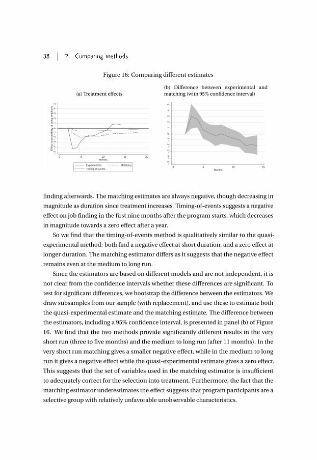
38 2. Comparing methods
Figure 16: Comparing different estimates
(a) Treatment effects
−.5
−.4
−.3
−.2
−.1
0.1
.2.3
.4.5
Effe
ct o
n pr
obab
ility
of b
eing
em
ploy
ed
0 5 10 15 20Months
Experimental MatchingTiming of events
(b) Difference between experimental andmatching (with 95% confidence interval)
−.5
−.4
−.3
−.2
−.1
0.1
.2.3
.4.5
0 5 10 15
Months
finding afterwards. The matching estimates are always negative, though decreasing in
magnitude as duration since treatment increases. Timing-of-events suggests a negative
effect on job finding in the first nine months after the program starts, which decreases
in magnitude towards a zero effect after a year.
So we find that the timing-of-events method is qualitatively similar to the quasi-
experimental method: both find a negative effect at short duration, and a zero effect at
longer duration. The matching estimator differs as it suggests that the negative effect
remains even at the medium to long run.
Since the estimators are based on different models and are not independent, it is
not clear from the confidence intervals whether these differences are significant. To
test for significant differences, we bootstrap the difference between the estimators. We
draw subsamples from our sample (with replacement), and use these to estimate both
the quasi-experimental estimate and the matching estimate. The difference between
the estimators, including a 95% confidence interval, is presented in panel (b) of Figure
16. We find that the two methods provide significantly different results in the very
short run (three to five months) and the medium to long run (after 11 months). In the
very short run matching gives a smaller negative effect, while in the medium to long
run it gives a negative effect while the quasi-experimental estimate gives a zero effect.
This suggests that the set of variables used in tbe matching estimator is insufficient
to adequately correct for the selection into treatment. Furthermore, the fact that the
matching estimator underestimates the effect suggests that program participants are a
selective group with relatively unfavorable unobservable characteristics.
2.9. Conclusion 39
2.9 Conclusion
Several methods are available when evaluating activation programs for unemployed
job seekers. In this paper we compare estimates from two methods, using estimates
exploiting a policy discontinuity as benchmark. These benchmark estimates rely on
exogenous variation in program participation, caused by budgetary problems of the
UI administration. We find that program participation reduces outflow to work in the
first couple of months after enrollment in the program with up to 40%-points, and has
no effect on job finding later on (10-18 months). These results are consistent with a
substantial lock-in effect often found in the literature.
We find that the matching and timing-of-events methods lead to slightly different
results. Both reproduce the negative short-run effect. However, the matching estimators
remain negative even after 18 months. The timing-of-events model estimate converges
to zero after 16 months. The discrepancy between the results suggests that even though
our data contain a very rich set of individual characteristics, there may still be additional
relevant unobserved characteristics.
It should be emphasized that our findings are based on a specific type of individuals
(those that were most likely to participate in the program), which we selected to increase
homogeneity of the sample as well as maximize the treated share before the policy
discontinuity. Both factors improve the estimators that we apply. This group has
relatively favorable characteristics though (native males with above average wages and
below average unemployment histories), which may affect the effect that we find. Our
findings can therefore not be generalized to the full population. Since this paper focuses
on the comparison of methods rather than estimating the average effect of the program
on the full population, we opted for restricting our sample in this manner.
We conclude that, especially in the case of activation programs, where selectivity in
participation is a large issue, even a large set of observed characteristics may not suffice
to correct for the bias. Some studies have used even richer data sets including “soft”
variables. For example Caliendo et al. (2014) include variables such as personality traits,
attitudes, expectations, and job search behavior and find that these play a significant
role in the selection of program participants. A useful next step would be to compare
non-experimental methods that include such information with (quasi-)experimental
evidence.


CHAPTER 3Providing advice to job seekers at
low cost: An experimental study
on on-line advice16
3.1 Introduction
Getting the unemployed back into work is an important policy agenda and a mandate
for most employment agencies. In most countries, a main tool to achieve this is to
impose requirements on benefit recipients to accept jobs beyond their occupation of
previous employment, at least after a few months.17 But little is said about how they
should obtain such jobs, and how one might advise them in the process. Despite a
substantial literature on the evaluation of active labor market policies, most studies
confound advice with monitoring and sanctions. In his famous meta-study on active
16This chapter is based on Belot et al. (2015)17In an OECD paper, Venn (2012) outlines that the requirement to accept jobs from other occupations
beyond the occupation of previous employment is one of the three main demands placed on the jobsearch of benefit recipients (the others are geographical distance, and job search requirements duringtraining). Countries differ by the length of time that benefit recipients can reject offers outside theiroccupation of previous employment: never (Australia, Denmark, Germany, Hungary, Ireland, Japan, NewZealand, Norway); no explicit time but dependent on previous work history (Canada, Czech Republic,Italy, Luxembourg, Poland, Slovak Republic, Sweden, Switzerland); less than six months (Austria, Estonia,Finland, France, Israel, Slovenia, United Kingdom, USA); more than six months (Belgium, Bulgaria,Cyprus, Malta, Netherlands, Spain); forever (Greece, Korea, Lithuania, Romania, Turkey). Like other labormarket policies, there is substantial variation and disagreement of optimal policy across countries.

42 3. Online jobsearch
labor market policies, Card et al. (2010) merge “job search assistance or sanctions
for failing to search" into one category.18 Ashenfelter et al. (2005a) assert a common
problem that experimental designs “combine both work search verification and a system
designed to teach workers how to search for jobs" and it is not clear which element is
responsible for their documented success. Only few studies, reviewed in the literature
section, have tried to fill the gap since, relying mostly on a mixture of labor-intensive
counseling services.
Our study aims to contribute by providing a randomized study that offers targeted
occupational advice to individual job seekers in a highly controlled and replicable low-
cost environment. To our knowledge our study is the first to use the expanding area of
online search to provide advice by re-designing the jobs search process on the web.
Internet-based job search is by now the predominant way of searching for jobs.19 We
asked professional programmers to set up two search platforms for internet-based job
search. One “standard” platform where job seekers themselves decide which keywords
and occupations to search for, similar to interfaces used on Universal Jobmatch (the
official job search platform provided by the UK Department of Work and Pensions) and
other commercial job search websites. The second “alternative” recommendation
platform asks job seekers about the occupation they are looking for - which can
coincide with the occupation of previous employment - and provides them with two lists
containing the most related occupations. The first is based on common occupational
transitions that similar people make and the second contains occupations for which
skill requirements are similar. Job seekers can then simply hit the search button and
are presented with all jobs in their geographic area that fall in any of these occupations.
They can also take a look at maps to see where jobs are easier to find.
The benefits of such an intervention are that it provides job search advice in a highly
controlled manner based on readily available statistical information, entails only advice
and no element of coercion (participants were free to continue with the “standard"
interface if they wanted to), and constitutes a low-cost intervention. It allows us to
tackle two questions. First, whether our implementation of advice changes how broad
18See the clarification in Card et al. (2009), p. 6.19Kuhn and Mansour (2014) document the wide use of the internet. Searchers who use the internet
nowadays seem to be more effective than those who do not, contrary to findings at the turn of themillennium where this path was still relatively new and used by only a minority. In the UK where ourstudy is based, roughly two thirds of job seekers (67%) and two thirds (64%) of employers now use theinternet for search and recruiting (ONS (2013), Pollard et al. (2012)). In Germany, 2/3 of all vacancies thatunemployed job seekers find are found through the internet (IAB (2010)).

3.1. Introduction 43
people search, where we define broadness as the average distance between occupational
classification codes of the vacancies that are considered.20 If it does, it allows us to
investigate the second question whether the induced increase in occupational breadth
increases job prospects. This is hard to assess without experimental variation because
people who search broadly tend to differ also in other dimensions.
We report our overall impact on the treatment group relative to the control group.
We also compare treatment and control in particular subgroups of obvious interest: our
study has more scope to affect people who search narrowly prior to our intervention,
and differential effects by duration of unemployment seem to be a major policy concern
as mentioned in the introductory paragraph. Overall, we find that our intervention
does expose job seekers to jobs from a broader set of occupations. And the number of
job interviews increases, mainly in jobs outside the job seeker’s core occupation. This
is driven predominantly by job seekers who otherwise search narrowly (compared to
similarly narrow searchers in the control group). Among these, the effects are driven by
those with above-median unemployment duration (more than 80 days). We take this as
indication that increasing the breadth of search increases job prospects, and targeted
job search assistance can be beneficial. It might not benefit everyone, though, and there
is some (insignificant) indication that it might discourage those who otherwise already
search broadly. We focus on job interviews as the number of jobs found are too limited
to allow statistical inference.21
In terms of detail of our setup, a crucial obstacle in this type of experimental research
is the two-sided nature of job markets: While one might rely on a limited number of job
seekers for initial investigation, a realistic job search environment relies crucially on
access to a large number of up-to-date vacancies. For this we convinced the largest UK
job search platform, Universal Jobmatch run by the Department of Work and Pensions,
to allow us access rights to its database of all live vacancies. Job seekers were recruited
in Edinburgh and we transformed the experimental laboratory into a job search facility
20The distance between two occupation codes is defined as zero when they are identical, 1 if theydiffer at the last digit, 2 if they differ at the second-to-last digit, up to 4 when they differ in all four digits.Alternative measures of broadness such as the Gini-Simpson index on a particular occupational digitprovide similar qualitative results, independent of the digit we are using.
21Attrition from one week to the next is low in our study, ranging from 2% to 4% per week, but is ofthe same order of magnitude as the reported job findings, which are also low in the current economicclimate. Since we do not know whether attrition is driven by those who find jobs and do not report backor those who simply drop out, inference is extremely difficult. In any case the numbers are too small toattribute statistical significance.

44 3. Online jobsearch
resembling those in “Employability Hubs” which provide computer access to job seekers
throughout the city.22 Participants were asked to search for jobs via our search platform
from computers within our computer laboratory once a week for a duration of 12
weeks. The advantage of this “field-in-the-lab" approach is tight control along three
dimensions: it ensures that job seekers indeed have access to a computer; any problems
or questions with our new experimental platform can be immediately handled; and
participants’ identities can be verified. The downside is a capacity restriction of 300
participants. As a twelve week panel this is a large number for experimental work but
limited relative to usual labor market survey data. As a first experimental study on
web-search design and advice we opted for more control and lower numbers.
All participants searched only with the “standard” interface for the first three weeks,
which provides a baseline on how occupationally “broad” participants search in the
absence of our intervention. Half of the participants continue with this interface
throughout the study, while the other half was offered to try an “alternative” interface
after the initial three weeks. The change was not previously announced, apart from a
general introductory statement to all participants that included the possibility to alter
the search engine over time. Instead of individual queries, our alternative interface
asks individuals about desired occupation and geographic region, and then provides
them at two clicks of a button with a list of alternative occupations (fist click) and all
vacancies that are within any of these occupations in the desired area (second click).
This provides advice in a simple and intuitive way that can be applied to all individuals
independent of their cognitive abilities. Obviously there is still room for the individual
to make choices, both regarding which of the suggested jobs to consider in more detail
and to apply for, as well as which desired occupation to name (which can be changed)
and whether to deselect some proposed occupations. But the process is much more
guided than the standard process where job seekers themselves have to come up with
search terms.
There are two reasons to worry that the “recommendation” interface might have
little effect. First, using it is not mandatory. Participants can opt to continue searching
with the standard interface and, thus, they have to be willing to use the recommendation
22Employability Hubs exist in several locations in Edinburgh through the cooperation Joined Up ForJobs comprising various non-for-profit organisations funded by the City of Edinburgh. They providecomputer rooms for job seekers around Edinburgh. They also provide other advice services. While oursetup is akin to their computer rooms, we never mentioned any connection while recruiting and wemade clear that we do not provide any actual job search advice.

3.1. Introduction 45
interface. All our results are reported independently of whether they use the interface
or not (intention to treat) since all participants used the interface at least once and
might have learned things that carry over even into their standard search activities.
Nevertheless, low participation might lead to limited effects. Second, the information
is taken from readily available sources and, therefore, might already be known to the
participants or to their advisers at the job centre.
Yet we do find that our intervention is effective in increasing the breath of search
and the number of job interviews, as mentioned earlier. We collect information both on
search success when searching in our computer facilities and on success through other
search channels. There is no crowding out between them. Both job interviews due to
search within our computer lab increase as well as interviews obtained through other
search channels, albeit only the sum is statistically significant. When we condition on
those who search narrowly in the first three weeks, each of these measures of interviews
increase significantly, indicating that the information that we provide on our interface
affects their search positively not just exclusively on our platform. This is also the group
for which we increase the occupational broadness of vacancy listings per week most
relative to their peers in the control group (though we seem to decrease the geographical
area they consider, possibly because they are now exposed to more suggestions within
closer geographic proximity). Also the occupational broadness of the jobs to which they
apply increases, although insignificantly, and their number of applications increases
significantly. The increase in the number of job interviews is particularly strong for those
who search occupationally narrow and have above median unemployment duration.
While it is straightforward why our information intervention has more scope to
broaden the perspective for individuals who otherwise search narrowly, it might
be less obvious why our effects are larger for those individuals with slightly longer
unemployment duration. A simple learning theory - which we advance theoretically
in a later section - can rationally account for this behaviour. If individuals who lost
their jobs deem it quite likely that they will obtain a job again in the same profession,
searching for jobs in this occupation might dominate search in alternative occupations
(i.e., they search narrowly). If the perceived difference between occupations is large, the
alternative occupations remain dominated even after we provide positive information
on some of them. After a few months, unsuccessful individuals learn that their chances
in their occupation of previous employment are lower than expected, and the perceived
difference with other occupations shrinks. Now alternative suggestions can render the

46 3. Online jobsearch
endorsed occupations attractive enough to be considered. Our intervention induces
search over a larger set of occupations and increases the number of interviews. One
can contrast this with the impact on individuals who already search broadly because
they find many occupations roughly equally attractive. They can rationally infer that
the occupations that we do not endorse are less suitable, and they stop applying there
to conserve search effort. Their broadness declines, but effects on job interviews are
theoretically ambiguous because search effort decreases but is better targeted. In the
data it is indeed the case that initially broad individuals in the treatment group become
occupationally narrower than comparable peers in the control group, but effects on job
finding are insignificant.
Our findings suggest concrete policy recommendations: targeted web-based advice
might be helpful to job seekers. This is particularly interesting because interventions
such as the one we evaluate have essentially zero marginal costs, and could be rolled
out on large scale without much burden on the unemployment assistance system.23
Clearly these results need to be viewed with caution. Evidence on job finding
probabilities are not conclusive given our limited sample size. Even if these were
conclusive, a true cost-benefit analysis would need to take into account whether
additional jobs are of similar quality (e.g. pay similarly and can be retained for similar
amounts of time). Such analysis is desirable, but requires a larger sample size with longer
follow-up, ideally based on access to administrative data. Larger roll-out in different
geographic areas would also be needed to uncover any general equilibrium effects,
which could reduce the effectiveness if improved search by some job seekers negatively
affects others, or could boost the effectiveness if firms react to more efficient search
with more job creation. We hope that future research in conjunction with conventional
large-scale operators of job search platforms will marry the benefits of our approach
with their large sample sizes.
The subsequent section reviews the related literature. Section 3.3 outlines the
institutional environment. Section 3.4 describes the experimental design, Section 3.5
the basics of our sample, and Section 3.6 our empirical analysis and findings. Section
23 The study itself cost roughly £100000, of which the largest part was compensation to participants,costs of programming, and salaries for research assistants. Designing the "recommendation" platformonly cost a fraction, and once this is programmed, rolling it out more broadly would have no furthermarginal cost of an existing platform such as Universal Jobmatch. Obviously, for researchers without anexisting client base, the marginal cost of attracting an additional participant to the study/website in thefirst place is nontrivial.

3.2. Related Literature 47
3.7 uses a simple model to illustrate the forces that might underlie our findings, and the
final section concludes.
3.2 Related Literature
The idea that search over different occupations is important in the job search process
has a long tradition both in the applied micro and in the macro-labor literature.24 But
as argued in the introductory paragraph, there are few experimental studies that focus
exclusively on providing advice, which limits our knowledge on the effectiveness of
information interventions in the labor market.25
Prior to our study the main focus of experimental investigation has been the
provision of counseling services by traditional government agencies and by new entrants
from the private sector. Behaghel et al. (2014) and Krug and Stephan (2013) provide
evidence from France and Germany that public counselling services are effective and
outperform private sector service provision, while Bennemarker et al. (2009) finds
similar overall effectiveness of the private and public counseling services in Sweden
with differential performance among specific subgroups. There are indications that
more advice would also be beneficial in the UK.26 General equilibrium effects are
24For example, Miller (1984), Neal (1999), Gibbons and Waldman (1999), Gibbons et al. (2005),Papageorgiou (2014) and Groes et al. (2015) document occupational mobility consistent with learningabout occupational skills. Moscarini and Thomsson (2007) and Kambourov and Manovskii (2008)highlight the high degree of occupational turnover in the US. Among others, Kambourov and Manovskii(2009) and Carrillo-Tudela and Visschers (2014) consider mobility and wage dynamics under occupation-specific skills and occupation-specific shocks. Barnichon and Figura (2014) and Sahin et al. (2014)point out that unequal market tightnesses across geography and occupations can contribute to overallaggregate unemployment, which opens the possibility that more balanced search can reduce aggregateunemployment.
25Ashenfelter et al. (2005a) apply indirect inference to ascertain the effectiveness of job search advice.They start by citing experimental studies from the US by Meyer (1995) which have been successfulbut entailed monitoring/sanctions as well as advice. Ashenfelter et al. (2005a) then provide evidencefrom other interventions that monitoring/sanctions are ineffective in isolation. Indirect inference thenattributes the effectiveness of the first set of interventions to the advice. Yet subsequent research on theeffects of sanctions found conflicting evidence: e.g., Micklewright and Nagy (2010) and Van den Berg andVan der Klaauw (2006) also find only limited effects of increased monitoring, while other studies such asVan der Klaauw and Van Ours (2013), Lalive et al. (2005) and Svarer (2011) find strong effects.
26Fieldwork by the UK government’s Behavioral Insights Team finds indications "that many claimants’first contact with the job centre focused entirely on claiming benefits, and not on finding work" (Gallagheret al. (2015)). This opens up the possibility that advice can indeed improve the search outcomes evenhere. Gallagher et al. (2015) themselves undertake a randomized trial. This trail includes many elementsincluding advice but also monitoring/sanctions: it re-focuses the initial meeting on search planning,introduces goal-setting and monitoring, and includes resilience building through creative writing. They

48 3. Online jobsearch
investigated in Crepon et al. (2013), who analyze a large scale rollout of private sector
counseling in France. While they cannot demonstrate such effects with statistical
significance, the point estimates on the effectiveness of counselling services reduces to
zero when general equilibrium effects are accounted for. The upshot of these studies is
their scale and the access to administrative data to assess their effects. The downside
is the large costs that range from several hundred to a few thousand Euro per treated
individual, and the "black box" of how advice is actually provided to individuals and how
it affects their job search. This complicates replication in other settings. Our study can
be viewed as complementary. It involves nearly zero marginal cost, the type of advice
is clearly focused on occupational information, it is standardized, its internet-based
nature makes it easy to replicate, and the detailed data on actual job search allow us to
study the effects not only on outcomes but also on the search process. Yet we have a
small and geographically confined set of participants and limited outcome measures.
Contemporaneously, Altmann et al. (2015) analyze the effects of a brochure that
they sent to a large number of randomly selected job seekers in Germany, containing
a paragraph of information and motivation on each of the following dimensions: i)
labor market conditions, ii) duration dependence, iii) effects of unemployment on life
satisfaction, and iv) importance of social ties. For this bundle, they find no significant
effect overall, but for those at risk of long-term unemployment they find a positive
effect between 8 months and a year after the brochure was sent. In our intervention
we find effects overall but also especially for individuals with longer unemployment
duration, even though we assess the intervention much closer in time to the actual
information provision. Their study has low costs of provision, is easily replicable, treated
a large sample, and has administrative data to assess success. On the other hand, it
is not clear which of the varied elements in the brochure drives the results, there are
no intermediate measures on how it affects the job search process, and the advice is
generic to all job seekers rather than specific to the occupations they are looking for.
Our study is also complementary to a few recent studies which study data from
commercial online job boards. It commenced with pioneering work on employer
find positive effects of their intervention, but cannot attribute it to the various elements. The resemblesfindings by by Launov and Waelde (2013) that attribute the success of German labor market reforms toservice restructuring (again both advice and sanctions) rather then benefit reductions. Another studyfor the UK conducted by Blundell et al. (2004) evaluates the "New Deal for the Young Unemployed".It provided job search assistance but it also included other elements, most notably a wage subsidy tounemployed youth.

3.2. Related Literature 49
behavior by Kuhn and Shen (2013b), but recent studies cited below shift attention to job
search behavior which is also the focus of our study.27 Their great advantage is the large
amount of data that is available. They have not investigated the role of advice, though,
nor can they rely on experimental variation. Another downside is a lack of information
about which other channels job seekers are using to search for jobs and why they are
leaving the site.28 We improve on the latter dimensions through our randomized design
and the collection of data on other search channels, albeit at the cost of a comparatively
small sample size.
Kudlyak et al. (2014) analyze U.S. data from Snagajob.com and find that job search
is stratified by educational attainment but that job seekers lower their aspirations
over time. Using the same data source, Faberman and Kudlyak (2014) investigate
whether the declining hazard rate of finding a job is driven by declining search effort.
They find little evidence for this. The data lacks some basic information such as
employment/unemployment status and reason for leaving the site, but they document
some patterns related to our study: Occupational job search is highly concentrated
and absent any exogenous intervention it broadens only slowly over time, with 60% of
applications going to the modal occupation in week 2 and still 55% going to the modal
occupation after six months.
Marinescu and Rathelot (2014) investigate the role of differences in market tightness
as a driver of aggregate unemployment. They discipline the geographic broadness of
search by using U.S search data from Careerbuilder.com. They concur with earlier
work that differences in market tightness are not a large source of unemployment. This
holds even in a robustness check that also allows for occupational segregation at the
2-digit code level. In their dataset search is rather concentrated, with the majority of
applications aimed at jobs within 25km distance and 82% of applications staying in
the same city (Core-Based Statistical Area), even if some 10% go to distances beyond
27Kuhn and Shen (2013b) investigate explicit gender discrimination in an environment where this islegal by looking at online data from Chinese job boards, and documents that many job advertisementsare explicitly gender-specific. Helleseter et al. (2014) extend this analysis to additional datasets fromChina and Mexico. Kuhn and Shen (2013a) document for a Chinese website that firms are reluctant tohire overqualified workers.
28Information on other search channels might be important if one is worried that effects on any onesearch channel might simply be shifts away from other search channels. Van den Berg and Van derKlaauw (2006) highlight this as the main reason for the ineffectiveness of monitoring the search activitiesof job seekers, since it mainly shifts sactivities out of hard-to-observe search channels like contactingfamily and friends into easy-to-observe search channels such as writing formal job applications. For ournon-coercive information intervention we do not find such crowding out.

50 3. Online jobsearch
100km.29 Using the same data source, Marinescu (2014) investigates equilibrium
effects of unemployment insurance by exploiting state-level variation of unemployment
benefits. The level of benefits affects the number of applications, but effects on the
number of vacancies and overall unemployment are limited. Marinescu and Wolthoff
(2014) document that job titles are an important explanatory variable for attracting
applications in Careerbuilder.com, that they are informative above and beyond wage
and occupational information, and that controlling for job titles is important to
understand the remaining role of wages in the job matching process. As mentioned,
none of these studies involve a randomized design.
To our knowledge, this is the first paper that undertakes job-search platform design
and evaluates it. The randomized setup allows for clear inference. While the rise in
electronic search will render such studies more and more relevant, the only other study
of search platform design that we are aware of is Dinerstein et al. (2014), who study a
change at the online consumer platform Ebay which changed the presentation of its
search results to order it more by price relative to other characteristics. This lead to a
decline in prices, which is assessed in a consumer search framework. While similar in
broad spirit of search design, the studies obviously differ substantially in focus.
3.3 Institutional Setting
We describe briefly the institutional settings relevant for job seekers in the UK during
the study. Once unemployed, a job seeker can apply for benefits (Job Seekers Allowance,
JSA), by visiting their local job centre. If they have contributed sufficiently through
previous employment, they are eligible for contribution-based JSA, which is £56.25 per
week for those aged up to age 24, and £72 per week for those aged 25 and older. These
benefits last for a maximum of 6 months. Afterwards - or in the absence of sufficient
contributions - income-based JSA applies, with identical weekly benefits but with extra
requirements. The amount is reduced if they have other sources of income, if they have
savings or if their partner has income. Once receiving JSA, the recipient is not eligible for
income assistance, however they may receive other benefits such as housing benefits.
29These numbers are based on Figure 5 in the 2013 working paper. Neither paper provides numberson the breath of occupational search. The "distaste" for geographical distance backed out in this work forthe US is lower than that backed out by Manning and Petrongolo (2011) from more conventional labormarket data in the UK, suggesting that labor markets in the UK are even more local.
3.3. Institutional Setting 51
JSA recipients should be available and actively looking for a job. In practice, this
implies committing to agreements made with a work coach at the job centre, such as
meeting the coach regularly, applying to suggested vacancies, participating in suggested
training. The work coach can impose sanctions on benefit payments in case of non-
compliance to any of the criteria.
In Figure 17 we present aggregate labor market statistics. In particular, figure (a)
show the unemployment rate in the UK and Edinburgh since 2011. The vertical line
indicates the start of our study. The unemployment rate in Edinburgh is slightly lower
than the UK average, and is rather stable between 2011 and 2014. These statistics are
based on the Labour Force Survey and may therefore be less precise. Therefore we
present the number of JSA claimants in the Edinburgh and the UK in panel (b), which
is an administrative figure and should be strongly correlated with unemployment. We
find that the number of JSA claimants is decreasing monotonically between 2012 and
2015, and that the Edinburgh and UK figures follow a very similar path. The number of
JSA claimants in Edinburgh during our study is approximately 9,000, such that the 150
participants per wave in our study are about 2% of the stock. The monthly flow of new
JSA claimants in Edinburgh during the study is around 1,800 (not shown in the graph).
Figure 17: Aggregate labor market statistics
(a) Unemployment rate
02
46
81
0U
ne
mp
loym
en
t ra
te (
%)
2011m1 2012m1 2013m1 2014m1
Edinburgh UK
(b) JSA claimants
04
00
80
01
20
01
60
0JS
A C
laim
an
ts U
K (
x1
00
0)
02
46
81
01
2JS
A C
laim
an
ts E
din
bu
rgh
(x1
00
0)
2012m1 2013m1 2014m1 2015m1
Edinburgh UK

52 3. Online jobsearch
3.4 Experimental Design
3.4.1 Basic setup
We conducted the study in the computer facilities of the School of Economics at the
University of Edinburgh over the course of the academic year 2013-14. Unemployed
job seekers were invited to search for jobs in our computer laboratory once a week
for a period of 12 weeks, or until they found a job. The study consisted of two waves:
wave 1 started in September 2013 and wave 2 started in January 2014. We conducted
sessions at six different time slots, on Mondays or Tuesdays at 10 am, 1 pm or 3:30 pm.
Participants chose a slot at the time of recruitment and were asked to keep the same
time slot for the twelve consecutive weeks.
Participants were asked to search for jobs using our job search engine (described
later in this section) for a minimum of 30 minutes.30 After this period they could
continue to search or use the computers for other purposes such as writing emails,
updating their CV, or applying for jobs. They could stay in our facility for up to two
hours. We emphasized that no additional job search support or coaching would be
offered.
All participants received a compensation of £11 per session attended (corresponding
to the government authorized compensation for meal and travel expenses) and we
provided an additional £50 clothing voucher for job market attire for participating in 4
sessions in a row.31
3.4.2 Recruitment Procedure and Experimental Sample
We recruited job seekers in the area of Edinburgh. The eligibility criteria for participating
to the study were: being unemployed, searching for a job for less than 12 weeks (a30The 30 minute minimum was chosen as a trade-off between on the one hand minimizing the effect
of participation on the natural amount of job search, while on the other hand ensuring that we obtainedenough information. Given that participants spent around 12 hours a week on job search, a minimum ofhalf an hour per week is unlikely to be a binding constraint on weekly job search, while it was a sufficientduration for us to collect data. Furthermore, similar to our lab participants, the participants in the onlinesurvey (who did not come to the lab and had no restrictions on how much to search) also indicate thatthey search 12 hours per week on average. Among this group, only in 5% of the cases the reported weeklysearch time is smaller than 30 minutes. In the study, the median time spent in the laboratory was 46minutes. We made sure that participants understood that this is not an expectation of their weekly searchtime, and that they should feel free to search more and on different channels.
31All forms of compensation effectively consisted of subsidies, i.e. they had no effect on the allowancesthe job seekers were entitled to. The nature and level of the compensation were discussed with the localjob centres to be in accordance with the UK regulations of job seeker allowances.

3.4. Experimental Design 53
Table 3: Recruitment and show-up of participants
Full sample Wave 1 Wave2Recruitment channel participants:
Job centres 86% 83% 89%Gumtree or other 14% 17% 11%
Sign up rate jobcentre for lab studya 43% 39% 47%c
Show up rate lab study 45% 43% 46%
Sign up rate jobcentre for online studya 60%Show up rate online studyb 21% 21% 21%a Of those people that were willing to talk to us about the study, this is the share thatsigned up for the study. b About a fourth of those that signed up for the online study had anon-existing email address, which partly explains the low show up rate. c Based on onlyone day of recruitment (see footnote 35).
criterion that we did not enforce), and being above 18 years old.32 We imposed no
further restrictions in terms of nationality, gender, age or ethnicity.
We obtained the collaboration of several local public unemployment agencies
(Jobcentres) to recruit job seekers on their premises. Their counsellors were informed
of our study and were asked to advertise the study. We also placed posters and
advertisements at various public places in Edinburgh (including libraries and cafes) and
posted a classified ad on a popular on-line platform (not limited to job advertisements)
called Gumtree. In Table 3 sign up and show up rates are presented. Of all participants,
86% were recruited in the Jobcentres. Most of the other participants were recruited
through our ad on Gumtree. We approached all visitors at the Jobcentres during two
weeks.33 Out of those we could talk to and who did not indicate ineligibility, 43%
percent signed up. Out of everyone that signed up, 45% showed up in the first week and
participated in the study. These figures display no statistically significant difference
between the two waves of the study.
We also conducted an online study, in which job seekers were asked to complete a
weekly survey about their job search. These participants did not attend any sessions,
but simply completed the survey for 12 consecutive weeks. This provides us with
32We do drop the observations on one participant from our sample because this participant had beenunemployed for over 30 years and was therefore an extraordinary outlier in our sample.
33Since most Job Seekers Allowance recipients were required to meet with a case worker once everytwo weeks at the Jobcentre, we were able to approach a large share of all job seekers.

54 3. Online jobsearch
descriptive statistics about job search behavior of job seekers in Edinburgh and it allows
us to compare the online participants with the lab participants. These participants
received a £20 clothing voucher for each 4 weeks in which they completed the survey.
The online participants were recruited in a similar manner as the lab participants, which
means most of them signed up at the Jobcentres.34 The sign up rate at the Jobcentres
was slightly higher for the online survey (58%), however out of those that signed up, only
21% completed the first survey. This was partly caused by the fact that about one-fourth
of the email addresses that were provided was not active.35
In section 3.5.1 we discuss in more detail the representativeness of the sample, by
comparing the online and the lab participants with population statistics.
3.4.3 Study Procedure
Participants were asked to register in a dedicated office at the beginning of each session.
At the first session, they received a unique username and password and were told to
sit at one of the computer desks in the computer laboratory. The computer laboratory
was the experimental laboratory located at the School of Economics at the University of
Edinburgh with panels separating desks to minimize interactions between job seekers.
They received a document describing the study as well as a consent form that we
collected before the start of the initial session (the form can be found in the Online
Appendix of Belot et al. (2015)). We handed out instructions on how to use the interface,
which we also read aloud (the instructions can be found in the Online Appendix of
Belot et al. (2015)). We always had assistance in the laboratory to answer questions.
We clarified that we were unable to provide any specific help for their job search, and
explicitly asked them to search as they normally would.
Once they logged in, they were automatically directed to our own website.36 They
were first asked to fill in a survey. The initial survey asked about basic demographics,
34Participants were informed of only one of the two studies, either the on-site study or the on-linestudy. The did not self-select into one or the other.
35 We asked the recruiters to write down the number of people they talked to and the number thatsigned up. Unfortunately these have not been separated for the online study and the lab study. In thefirst wave there were different recruiters for the two studies, such that we can compute the sign up sharesseparately. In the second wave we asked assistants to spend parts of their time per day exclusively on thelab study and parts exclusively on the online study, so we only have sign-ups for the total number. Oneday was an exception, as recruitment was done only for the lab study on this day, such that we can reporta separate percentage based on this day.
36www.jobsearchstudy.ed.ac.uk

3.4. Experimental Design 55
employment and unemployment histories as well as beliefs and perceptions about
employment prospects. From week 2 onwards, they only had to complete a short weekly
survey asking about job search activities and outcomes. For vacancies saved in their
search in our facility we asked about the status (applied, interviewed, job offered).
We asked similar questions about their search through other channels than our study.
The weekly survey also asked participants to indicate the extent to which they had
personal, financial or health concerns (on a scale from 1 to 10). The complete survey
questionnaires can be found in the Online Appendix of Belot et al. (2015).
After completing the survey, the participants were re-directed towards our search
engine and could start searching. A timer located on top of the screen indicated how
much time they had been searching. Once the 30 minutes were over, they could end the
session. They would then see a list of all the vacancies they had saved and were offered
the option of printing these saved vacancies. This list of printed vacancies could be
used as evidence of required job search activity at the Jobcentre. It was, however, up
to the job seekers to decide whether they wanted to provide that evidence or not. We
also received no additional information about the search activities or search outcomes
from the Jobcentres. We only received information from the job seekers themselves.
This absence of linkage was important to ensure that job seekers did not feel that their
search activity in our laboratory was monitored by the employment agency. They could
then leave the facilities and receive their weekly compensation.37 Those who stayed
could either keep searching with our job search engine or use the computer for other
purposes (such as updating their CV, applying on-line or using other job search engines).
We did not keep track of these other activities. Once participants left the facility, they
could still access our website from home, for example in order to apply for the jobs they
had found.
3.4.4 Experimental Treatments
We introduce experimental variation through changes in the job search engine. All
participants started using a “standard" search interface. Then from week four onwards
half of the participants were allocated an “alternative" search interface which provided
recommendations of alternative occupations in which they could search for jobs. We
37Participants were of course allowed to leave at any point in time but they were only eligible to receivethe weekly compensation if they had spent 30 minutes searching for jobs using our search engine.

56 3. Online jobsearch
now explain in more detail how each of these interfaces work, and how we assigned
them.
The Standard Interface
We designed a job search engine in collaboration with the computer applications team
at the University of Edinburgh. It was designed to replicate the search options available
at the most popular search engines in the UK (such as monster.com and Universal
Jobmatch), but allowing us to record precise information about how people search for
jobs (what criteria they use, how many searches they perform, what vacancies they
click on and what vacancies they save), as well as collecting weekly information (via
the weekly survey) about outcomes of applications and search activities outside the
laboratory.
The search engine uses a database of real job vacancies, which is identical to those
provided on the government website Universal Jobmatch. This is the largest in the
UK in terms of the number of vacancies. This is a crucial aspect in the setup of the
study, because results can only be trusted to resemble natural job search if participants
use the lab sessions for their actual job search. The large set of available vacancies
combined with our carefully designed job search engine assures that the setting was
as realistic as possible. Panel (a) of Figure 18 shows the number of posted vacancies
available through our search engine in Edinburgh and in the UK for each week of the
study (the vertical line indicates the start of wave 2). Each week there are between
800 and 1600 new vacancies posted in the Edinburgh. Furthermore, there is strong
correlation between vacancy posting in Edinburgh and the UK. In panel (b) the total
number of active vacancies in the UK is shown over the second half of 2013 and 2014.38
As a comparison the total number of active vacancies in the database used in the study
in both waves is shown. It suggests that the database contains over 80% of all UK
vacancies, which is a very extensive coverage compared to other online platforms.39 It
is well-known that not all vacancies on online job search platforms are genuine, so the
38Panel (b) is based on data from our study and data from the Vacancy Survey of theOffice of National Statistics (ONS), dataset “Claimant Count and Vacancies - Vacancies", url:www.ons.gov.uk/ons/rel/lms/labour-market-statistics/march-2015/table-vacs01.xls
39For comparison, the largest US jobsearch platform has 35% of the official vacancies; see Marinescu(2014), Marinescu and Wolthoff (2014) and Marinescu and Rathelot (2014). The size difference might bedue to the fact that the UK platform is run by the UK government.

3.4. Experimental Design 57
Figure 18: Number of vacancies
(a) Posted vacancies in our study
040
000
8000
012
0000
1600
00V
acan
cies
pos
ted
per
wee
k in
UK
040
080
012
0016
00V
acan
cies
pos
ted
per
wee
k in
Edi
nbur
gh
0 5 10 15 20 25Experiment week
Edinburgh UK
(b) Active vacancies in our study and in UK
020
0000
4000
0060
0000
2013w26 2014w1 2014w26 2015w1week
Total vacancies in UK Vacancies in study (wave 1)Vacancies in study (wave 2)
actual number might be somewhat lower.40 We introduced ourselves a small number of
“fake" vacancies (about 2% of the database) for a separate research question (addressed
in a separate paper). Participants were fully informed about this. They were told that
“we introduced a number of vacancies (about 2% of the database) for research purposes
to learn whether they would find these vacancies attractive and would consider applying
to them if they were available".41 This small number is unlikely to affect job search, and
there is no indication of differential effects by treatment group.42
When using the standard interface, participants can search using various criteria
(keywords, occupations, location, salary, preferred hours), but do not have to specify all
of these. Once they have defined their search criteria, they can press the search button
at the bottom of the screen and a list of vacancies fitting their criteria will appear. The
40 For Universal Jobmatch evidence has been reported on fake vacancies covering 2% of the stockposted by a single account (Channel 4 (2014)) and speculations of higher total numbers of fake jobscirculate (Computer Business Review (2014)). Fishing for CV’s and potential scams are common on manysites, including Carreerbuilder.com (The New York Times (2009a)) and Craigslist, whose chief executive,Jim Buckmaster, is reported to say that “it is virtually impossible to keep every scam from traversing anInternet site that 50 million people are using each month" (The New York Times (2009b)).
41Participants were asked for consent to this small percentage of research vacancies. They wereinformed about the true nature of such vacancies if they expressed interest in the vacancy before anyactual application costs were incurred, so any impact was minimized. We exploit this experimentalvariation in vacancy postings in a separate paper.
42In an exit survey the vast majority of participants (86%) said that this did not affect their searchbehavior, and this percentage is not statistically different in the treatment and control group (p-value0.99). This is likely due to the very low numbers of fake vacancies and to the fact that fake advertisementsare common in any case to online job search sites (see footnote 40) and that this is mentioned to jobseekers in many search guidelines (see e.g. Joyce (2015)).

58 3. Online jobsearch
information appearing on the listing is the posting date, the title of the job, the company
name, the salary (if specified) and the location. They can then click on each individual
vacancy to reveal more information. Next, they can either choose to “save the job" (if
interested in applying) or “do not save the job" (if not interested). If they choose not to
save the job, they are asked to indicate why they are not interested in the job from a list
of possible answers.
As in most job search engines, they can modify their search criteria at any point
and launch a new search. Participants had access to their profile and saved vacancies
at any point in time outside the laboratory, using their login details. They could also
use the search engine outside the laboratory. We recorded all search activity taking
place outside the lab. This is however only a very small share compared to the search
activities performed in the lab.
The Alternative Interface
We designed an alternative interface again in collaboration with the Applications team
at the University of Edinburgh. This interface aims to reduce informational frictions
and to expose job seekers to the set of vacancies that is likely to be relevant to them.
The interface consists of two alterations. First, based on their profile it suggests possible
occupations job seekers may be suited for. Second, it provides visual information on the
tightness of the labor market for broad occupational categories in regions in Scotland.
Furthermore, the search engine was somewhat restricted in the criteria that could be
specified (it only allows to use occupation and radius as search criteria).
When using the alternative interface, participants were asked to specify their
preferred occupation. They could change their preferred occupation at any time over
the course of the study. The preferred occupation was then matched to a list of possibly
suitable occupations using two different methodologies. The first uses information
from the British Household Panel Survey and from the national statistical database
of Denmark (because of larger sample size).43 Both databases follow workers over
time and record in what occupation they are employed. We then match the indicated
preferred occupation to the most common occupations to which people employed in
the preferred occupation transition to.44
43The name of the database is IDA - Integrated Database for Labour Market Research administered byStatistics Denmark. We are grateful to Fayne Goes for providing us with the information.
44For each occupation we created a list of the 3 to 5 most common transitions; at least 3 if availableand at most 5 if more than 5 were available. These consist of occupations that are in both datasets in

3.4. Experimental Design 59
The second methodology uses information on transferable skills across occupations
from the US based website O*net, which is an online “career exploration" tool sponsored
by the US department of Labor, Employment & Training Administration. For each
occupation, they suggest up to 10 related occupations that require similar skills. We
retrieved the related occupations and presented the ones related to the preferred
occupation as specified by the participant.
Once participants have specified their preferred occupation, they could then click
“ Save and Start Searching” and were taken to a new screen where a list of suggested
occupations was displayed. The occupations were listed in two columns: The left
column suggests occupations based on the first methodology (based on labor market
transitions). The right column suggests occupations based on the second methodology
(O*net related occupations). Participants were fully informed of the process by which
these suggestions came about, and could select or unselect the occupations they wanted
to include or exclude in their search. By default all were selected. If they then click the
“search" button, the program searches through the same underlying vacancy data as in
the control group but selects all vacancies that fit any of the selected occupations.45
We also provided information about how competitive the labor market is for a given
set of occupations. We constructed “heat maps" that use recent labor market statistics
for Scotland and indicate visually (with a colored scheme) where jobs may be easier
to get (because there are many jobs relative to the number of interested job seekers).
These maps were created for each broad occupational category (two-digit SOC codes).46
Participants could access the heat maps by clicking on the button “heat map" which
was available for each of the suggested occupations based on labor market transitions.
the top-10 common transitions. If there are less than 3 of these, we added the most common transitionsfrom each of the datasets.
45Occupations in O*net have a different coding and description and have a much finer categorizationthan the three-digit occupational code available in the British Household Panel Survey (BHPS) and inUniversal Jobmatch vacancy data. We therefore asked participants twice for their preferred occupation,once in O*net form and BHPS form. The query on the underlying database relies on keyword search,taking the selected occupations as keywords, to circumvent problems of differential coding.
46These heat maps are based on statistics provided by the Office for National Statistics, (NOMIS,claimant count, by occupations and county, see https://www.nomisweb.co.uk/). We created the heatmaps at the two-digit level because data was only available on this level. Clearly, this implies that thesame map is offered for many different 4-digit occupations, and job seekers might see the same mapseveral times. Obviously a commercial job search site could give much richer information on the numberof vacancies posted in a geographic area and the number of people looking for particular occupations inparticular areas. An example of one of the heat maps is can be found in the Online Appendix of Belotet al. (2015).

60 3. Online jobsearch
So they could check them for each broad category before actually performing a search,
not for each particular vacancy.
Participants in the treatment group received a written and verbal instruction of
the alternative interface (see Online Appendix of Belot et al. (2015)), including how
the alternative recommendations were constructed, in the fourth week of the study
before starting their search. For them, the new interface became the default option
when logging on. It should be noted, though, that it was made clear to participants
that using the new interface was not mandatory. Rather, they could switch back to the
previous interface by clicking a button on the screen indicating “use old interface". If
they switched back to the old interface, they could carry on searching as in the previous
weeks. They could switch back and forth between new and old interface. This ensures
that we are not restricting choice, but rather offer advice.
Randomization
From week 4 onwards, we changed the search interface to the alternative interface
for a subset of our sample. Participants were randomized into control (no change in
interface) and treatment group (alternative interface) based on their allocated time slot.
We randomized each time slot into treatment and control over the two waves, to avoid
any correlation between treatment status and a particular time slot. Table 4 illustrates
the randomization.
Table 4: Randomization scheme
Wave 1 Wave 2Monday 10 am Control TreatmentMonday 1 pm Treatment ControlMonday 3:30 pm Control TreatmentTuesday 10 am Treatment ControlTuesday 1 pm Control TreatmentTuesday 3:30 pm Treatment Control

3.5. Background Data on our Sample 61
3.5 Background Data on our Sample
3.5.1 Representativeness of the sample
Since the participants were not randomly selected from the population of job seekers
in Edinburgh, one may worry that the sample consists of a selective group that differs
from the general population. To provide some indication of the degree of selection,
we compare characteristics of the participants to the online survey participants, and
to aggregate statistics of job seekers available from The Office of National Statistics
(NOMIS). These descriptive statistics are presented in Table 5. The first four columns
show the mean, standard deviation, minimum and maximum for the lab participants,
while the next four columns show the same statistics for the online survey participants.
In column 9, the p-value of a two-sided t-test for equal means is shown. Finally, in
column 10 aggregate statistics of job seekers in Edinburgh are shown, for the variables
for which these are available.47
Demographic variables, based on the first week baseline survey, show that 43% of
the lab participants are female, the average age is 36 and 43% have some university
degree. 80% classify themselves as ‘white’ and 27% have children. The online survey
participants differ somewhat in composition: they are more likely to be female, they
are slightly younger and they have less children. When comparing these statistics to
aggregate statistics of Edinburgh job seekers, we find that we oversample women and
non-whites, while the average age is very similar.
The lower part of Table 5 shows variables related to job search history, also based on
the first week baseline survey. The lab participants have on average applied to 64 jobs,
which lead to 0.48 interviews and 0.42 job offers.48 Only 20% received at least one offer.
Mean unemployment duration at the start of the study is 260 days, while the median is
80 days. About three-fourth of the participants had been unemployed for less than half
a year. Participants typically receive job seekers allowance and housing allowance. The
online survey participants are not significantly different on most dimensions, except
that they attended more job interviews.
47Source: Office for National Statistics: NOMIS Official Labour Market Statistics. Dataset: ClaimantCount conditional on unemployment duration< 12 months, average over the duration of the study. Werestrict attention to durations of less than 12 months to equalize the median unemployment durationbetween the NOMIS query and our dataset.
48We censor the response to the survey question on the number of previous job offers at 10.

62 3. Online jobsearch
We also compare job search behavior of participants in our study with the online
survey participants. The online survey includes a question asking for the weekly number
of applications sent and the weekly number of job interviews. We compare the control
group lab participants to the online survey participants to assess whether participation
in the study affects the participants. When using data on applications and interviews in
our study, we assign both of these to the week in which search activity was performed
that lead to either to these. On average this implies that applications are assigned to
search activity one week before the application was send, while interviews are assigned
to search activity two weeks before the interview is reported. The average number of
applications are shown in panel (a) of Figure 19 and the average number of interviews in
panel (b) of Figure 19. For lab participants we observe both the number of applications
from job search in the lab, and the number of applications reported through other
job search activities. The number of applications outside the lab is quite similar to
the number reported by the online participants, while the sum of the two types of
applications for lab participants is somewhat higher than for the online participants. In
panel (b) we find that the sum of interviews in- and outside the lab is very similar to the
number reported by the online participants. The average number of weekly interviews
is 0.47 for lab participants and 0.42 for online participants and these numbers are not
statistically different (p-value 0.23).
Figure 19: Jobsearch behavior online and lab participants
(a) Applications
03
69
12A
pplic
atio
ns
2 4 6 8 10 12Week
Online survey participants Lab participants: in labLab participants: outside lab
(b) Interviews
0.2
.4.6
Inte
rvie
ws
2 4 6 8 10Week
Online survey participants Lab participants: in labLab participants: outside lab

3.5. Background Data on our Sample 63
Table 5: Characteristics of lab participants and online survey participants (based onthe first week initial survey)
Lab participants Online survey T-testa Pop.b
mean sd mean sd pvalDemographics:
gender (%) 43 50 52 50 .09 33age 36 12 34 12 .08 35high educ (%) 43 50 43 50 1.00white (%) 80 40 77 42 .43 89number of children .53 1 .28 .57 .02couple (%) 23 42 23 42 .96any children (%) 27 45 23 42 .41
Job search history:vacancies applied for 64 140 75 187 .53interviews attended .48 .84 2.7 4 .00jobs offered .42 1.1 .51 1.6 .52at least one offer (%) 20 40 24 34 .36days unempl. (mean) 260 620 167 302 .15 111days unempl. (median) 80 118 81less than 183 days (%) 76 43 75 44 .76less than 366 days (%) 85 35 91 28 .13job seekers allowance (£) 52 75 58 42 .49housing benefits (£) 64 129 48 95 .36other benefits (£) 14 65 12 56 .81
Observations 295 103a P-value of a t-test for equal means of the lab and online participants. b Average characteristics ofthe population of job seeker allowance claimants in Edinburgh over the 6 months of study. Thenumbers are based on NOMIS statistics, conditional on unemployment duration up to one year. c
High educated is defined as a university degree.

64 3. Online jobsearch
Table 6: Characteristics of the treatment and control group
Control group Treatment group T-testmean sd mean sd pval
Demographics:female (%) 44 50 41 49 .67age 36 11 37 12 .53high educ (%) 43 50 42 50 .85survey qualification level 4.2 1.9 4.5 1.9 .27white (%) 80 40 81 40 .88number of children .64 1.1 .40 .83 .04couple (%) 25 44 21 41 .37any children (%) 30 46 25 43 .37
Job search history:vacancies applied for 74 154 53 122 .21interviews attended .41 .63 .56 1 .13jobs offered .37 .96 .49 1.2 .35at least one offer (%) 19 40 21 41 .77days unemployed (mean) 286 668 231 563 .45days unemployed (median) 80 78less than 183 days .75 .44 .78 .42 .54less than 366 days .85 .36 .86 .34 .64job seekers allowance (£) 48 41 56 101 .43housing benefits (£) 64 123 63 136 .96
Weekly search activities in weeks 1-3:listed 498 396 488 377 .82saved 10 10 11 12 .56applied 3.3 5.8 2.5 4.3 .18interview .09 .34 .09 .24 .84applications other 9.2 11 7.5 8.3 .15interviews other .53 .70 .49 .79 .69broadness listeda 3.2 .61 3.2 .57 .73broadness applieda 3 .95 3.2 .90 .36hours spendb 11 8.2 12 10 .12concern health (scale 1-10) 1.5 2.5 1.7 2.7 .46concern financial (scale 1-10) 7.3 2.6 6.9 3.1 .30concern competition (scale 1-10) 7.4 2.3 7.2 2.2 .52met caseworker (%) 31 37 29 39 .61
Observations 155 140
Demographics and job search history values are based on responses in the baseline survey fromthe first week of the study. Search activities are mean values of search activities over the first 3weeks of the study. a Occupational broadness, as defined in section 3.5.4. b The number of hoursspend on job search per week.

3.5. Background Data on our Sample 65
3.5.2 Treatment and Control Groups
In order to evaluate the effect of the alternative interface on job search behavior and
outcomes we compare treated and non-treated individuals. Both of these groups
used the same interface in the first three weeks, and the alternative interface was only
provided to the treatment group from week 4 onwards. This means that we can use
the information from the first three weeks to correct for fixed differences between
treated and control group individuals. In principal this should not be necessary though,
since the treatment was assigned randomly. Still, the group fixed effects will increase
precision. In Table 6 we compare characteristics of the treatment and control group to
ensure that the composition of the groups is balanced.49
We compare the treated and control group on the same set of demographic and job
search history variables as in Table 5, and additionally we compare job search behavior
in our study over weeks 1-3. For demographic and job search history variables, only
one out of 32 t-tests suggests a significant difference, which is the average number of
children. In terms of job search behavior in our study over the first three weeks, we
find that the control group lists on average 498 vacancies, of which 10 are saved. Out
of these, participants report to have applied to 3 and eventually get an interview in
0.09 cases. Furthermore, they report about 8 weekly applications through channels
outside our study, leading to 0.03 interviews on average. For each set of vacancies
(listed, viewed, saved, applied) we compute a measure of occupational broadness (see
subsection 3.5.4), of which the average values are also shown in the table. Participants
in the control group report 11 hours of weekly job search in addition to our study. In the
weekly survey, participants were also asked to rate to what extend particular problems
were a concern to them. On average, health problems are not mentioned as a major
concern, while financial problems and strong competition in the labor market seem to
be important. Finally, about 30% met with a case worker at the Jobcentre in a particular
week. The values for job search behavior of the treatment group are very similar, and
never differ significantly.
49For example, it could be the case that by expressing a strong preference for a particular time slot,participants self-select into groups. Since we switch around the treatment assignment of groups in thesecond wave (see Table 4), this is unlikely to be problematic though.

66 3. Online jobsearch
3.5.3 Attrition
The study ran for 12 weeks, but job seekers could obviously leave the study earlier
either because they found a job or for other reasons. Thus, attrition is an inherent
feature of our study, and the experimental intervention could have affected attrition
rates. Differential attrition driven by differences in job finding across groups is of course
of direct interest, but it also introduces challenges for the empirical analysis of search
behavior, as both samples may not remain comparable over the 12 weeks.
We present attrition in panel (a) of Figure 20, for the control and treatment groups
(including 95% confidence intervals).50 An exit from the study is defined to occur in the
week after the last session in which the individual attended a lab session, irrespective of
the reason for exiting the study. We find that about 50% of the participants continue
until the end of the study, and this percentage is very similar in the control and treatment
group. The difference between the two curves is not significant at any duration. Of
course, it is important to point out that even if we find attrition of similar magnitude
in the treatment and control groups, we could still have systematic differences in
unobservables over time because there may be heterogeneity in how each interface
affects job seekers. We will come back to this issue in the empirical analysis.
Whenever participants dropped out, we followed up on the reasons for dropping
out. In case they found a job, we asked for details, and in many cases we were able to
obtain detailed information about the new job. Since job finding is a desirable outcome
related to the nature of our study, we also present attrition excluding job finding in
panel (b) of Figure 20. Here we present the number of participants leaving the study
per week due to reasons other than finding employment. In most weeks, we lose 2 to 4
participants, and again, these numbers are very similar in control and treatment group.
The apparent lack of selection is on the one hand helpful to study how the
intervention may have affected search outcomes, on the other hand, it already hints that
our intervention may not have affected the rather low job finding rates in a statistically
significant way. We will come back to the analysis of drop out and job finding in more
detail in section (3.6.4).
50The graph shows Kaplan-Meier estimates of the survival functions of the groups.

3.5. Background Data on our Sample 67
Figure 20: Attrition of participants in the standard and alternative interface groups
(a) Kaplan-Meier survival functions (exits includejob finding), with 95% confidence intervals
0.2
5.5
.75
1P
art
icip
an
ts
1 3 5 7 9 11Week
Standard interface Alternative interface
(b) Attrition per week (excluding job finding)
02
46
81
0P
art
icip
an
ts
1 3 5 7 9 11Week
Standard interface Alternative interface
3.5.4 Measuring occupational and geographical broadness
We are interested in the effect of providing information about suitable occupations as
well as geographical labor market statistics. Measuring such effects requires defining
occupational and geographical broadness measures. In this subsection we provide
definitions of the measures that are used in the empirical analysis. All measures are
defined on the set of vacancies retrieved in a given week, independent of whether they
arose due to many independent search queries or few comprehensive queries.
For occupational broadness we focus on the UK Standard Occupational Classifi-
cation code (SOC code) of a particular vacancy, which consists of four digits.51 The
structure of the SOC codes implies that the more digits two vacancy codes share, the
more similar they are. Our measure of diversity within a set of vacancies is based on
this principle, defining for each pair within a set the distance in terms of the codes. The
distance is zero if the codes are the same, it is 1 if they only share the first 3 digits, 2 if
they only share the first 2 digits, 3 if they share only the first digit and 4 if they share no
digits. This distance, averaged over all possible pairs within a set, is the measure that we
use in the empirical analysis.52 Note that it is increasing in broadness (diversity) of a set
51The first digit of the code defines the “major group" , the second digit defines the “sub-major group",the third digit defines the “minor group" and the fourth digit defines the “unit group" which providesa very specific definition of the occupation. Some examples are “Social science researchers" (2322),“Housekeepers and related occupations" (6231) and “Call centre agents/operators" (7211).
52Our results are robust to using the Gini-Simpson index as an alternative broadness measure.

68 3. Online jobsearch
of vacancies. We compute this measure for the set of listed and applied vacancies in
each week for each participant.
For geographical broadness we use a simple measure. Since a large share of searches
restricts the location to Edinburgh, we use the weekly share of a participants searches
that goes beyond Edinburgh as the measure of geographical broadness.53
3.6 Empirical Analysis
We now turn to the empirical analysis. Ultimately we want to find out whether our
intervention improves labor market prospects. Our data allow us to examine each step
of the job search process: the listing of vacancies to which job seekers are exposed, the
vacancies they apply to, the interviews they get and finally, and whether they find a
job. Clearly, the ultimate outcome variable we care about is actual job finding, as well
as characteristics of the job found (occupation, wage, duration, etc.), which would be
important to evaluate the efficiency implications of such an intervention. Unfortunately
the information we have on job finding is limited; job finding is relatively rare, and our
information on job finding is rather noisy, so we should be cautious when interpreting
the results. This is why we focus most of the analysis on the steps preambling job
finding, specifically vacancy listings, applications and interviews. Listed vacancies are
the direct result of the search criteria used by the job seeker and therefore are the most
immediate measure of search behavior. Applications provide a more reliable measure of
the job seekers’ interest in the vacancies.54 Interviews are the next measure of interest
and the next best variable to indicate interest of the employers, and since there are a
lot more interviews than jobs found, it is the best indicator we have of labor market
prospects. We will briefly discuss the evidence on job finding at the end of this section.
In the weekly survey that participants complete before starting to search, we
ask about applications and interviews through channels other than our study. The
intervention may affect these outcomes as well, since the information provided in
the alternative interface could influence people’s job search strategies outside the lab.
Therefore we also document the weekly applications and interviews through other
channels as outcome variables. We start with presenting the econometric specification.
53Note that the direct surroundings of Edinburgh contain only smaller towns. The nearest large city isGlasgow, which takes about 1-1.5 hours of commuting time.
54We also constructed measures of broadness based on the viewed and saved vacancies. The resultswere qualitatively similar to the those obtained for the listed and applied vacancies. They are availableupon request.

3.6. Empirical Analysis 69
3.6.1 Econometric speci�cation
Our data is a panel and our unit of observation is at the week/individual level. That is,
we compute a summary statistic for each individual of her search behavior (vacancies
listed, applications, interviews) in a given week. Since it is a randomized controlled
experiment in which we observe individuals for three weeks before the treatment starts,
the natural econometric specification is a model of difference-in-differences. To take
account of the panel structure we include individual random effects. We have estimated
a fixed effects model and performed a Hausman test for each of the main specifications.
In none of the cases we could reject that the random effects model is consistent, such
that we decide in favor of the random effects model for increased precision. Specifically,
we can compare a variable measuring an outcome (Y ) in the control and treatment
group before and after the week of intervention, controlling for week fixed effects (αt ),
time–slot × wave fixed effects (δg ) and a set of baseline individual characteristics (Xi )
to increase the precision of the estimates. The treatment effect is captured by a dummy
variable (Ti t ), equal to 1 for the treatment group from week 4 onwards. The specification
we propose is:
Yi t =αt +δg +γTi t +Xiβ+ηi +εi t (3.1)
where i relates to the individual, t to the week and ηi +εi t is an error term consisting
of an individual specific component (ηi ) and a white noise error term (εi t ). Individual
characteristics Xi include gender, age and age squared, unemployment duration
and unemployment duration squared55 and dummies indicating a short expected
unemployment duration, financial concerns, being married or cohabiting, having
children, being highly educated and being white.
As mentioned earlier, one important challenge with such approach has to do with
attrition. If there is differential attrition between treatment and control groups, it
could be that both groups differ in unobservables following the treatment. Differential
attrition is of course particularly plausible because our treatment could have affected
job finding and therefore study drop out. We proceed in two ways to address this
potential concern. First, we documented in Section 3.5.3 attrition across treatment
and control groups and found no evidence of asymmetric attrition. Second, our panel
structure allows us to control for time-invariant heterogeneity and use within-individual
variation. When we estimate a random and fixed effects model, the Hausman test fails
55Unemployment duration is defined as the reported duration at the start of the study.

70 3. Online jobsearch
to reject the latter. Since the treatment itself is assigned at the group-level it is unlikely to
be correlated with unobserved individual characteristics. However, differential attrition
could create correlation between unobservable individual characteristics and would
therefore lead to rejection of the random-effects model. The fact that we can never
reject this model is thus an indication that there is no (strong) differential attrition
between treatment and control groups.
We summarize in Table 7 the outcome variables of interest. For listed vacancies
and applications we look at broadness (occupational and geographical) and the
number. For interviews we only look at the number, since the number is too small
to compute informative broadness measures. As an alternative, we asked individuals
at the beginning of the study about three “core” occupations in which they are looking
for jobs, and we can estimate separate treatment effects for interviews in core and
non-core occupations. For the number of applications and interviews we also look at
activity outside the lab. Note that applications and interviews through activity in lab are
assigned to the week in which the search activity was performed. A similar correction
is made for applications and interviews through other channels, which is described in
more detail in the relevant sections.
Another important aspect relevant for the econometric specification is the potential
heterogeneity of effects across individuals. Given the nature of the intervention, it
is likely that the treatment affects different individuals differentially. In order for
our intervention to affect job prospects, it has to open new search opportunities
Table 7: Outcome variables
Search activity Search activityin the lab outside the lab
Listed vacanciesOccupational Broadness
pGeographical Broadness
pNumber
pApplications
Occupational Broadnessp
Geographical Broadnessp
Numberp p
InterviewsNumber
p pCore and non-core occupations
p

3.6. Empirical Analysis 71
to participants and participants have to be willing to pursue those opportunities.
Participants may differ in terms of their search strategies. We expect our intervention
to broaden the search for those participants who otherwise search narrowly, which we
will measure by their search in the weeks prior to the intervention. For those who are
already searching broadly in the absence of our intervention it is not clear whether we
increase the breadth of their search. We therefore estimate heterogeneous treatment
effects by initial broadness.56
Second, the willingness to pursue new options depends on the incentives for job
search, which change with unemployment duration for a variety of reasons. Longer-
term unemployed might be those for whom the search for their preferred jobs turned out
to be unsuccessful and who need to pursue new avenues, while they are also exposed
to institutional incentives to broaden their search (the Jobcentres require job seekers
to become broader after three months). Note again that we are always comparing
otherwise identical individuals in the treatment and control groups, so the incentives
to broaden their search by themselves would not be different, but the information we
provide to achieve this differs. We therefore also interact the treatment effect with
unemployment duration. In the subsequent section we provide a simple theoretical
model formalizing the channels that may explain differential effects.
Note that since we did not force job seekers to use the alternative interface, our
intervention is an intention-to-treat. Panel (a) of Figure 21 plots the fraction of users
of the alternative interface over the 12 weeks. On average we find that around 50%
of the treated participants use the alternative interface over the 8 weeks and this
fraction remains quite stable throughout. This does not mean that only 50% of the
treatment group is treated though because all participants in the treatment group used
the alternative interface at least once and were therefore exposed to recommendations
and suggestions based on their profile. It could be that they used this information while
reverting back to searching with the standard interface.
Bearing this in mind, we now document the effects of the intervention on the various
steps of the search process. We will present the results on the treatment effect only (γ) as
well as the interaction effects between the treatment and the subgroups of interest, for
the sake of brevity. For the amount of search activity we report the full results including
all other covariates in Table 20 in the Appendix.
56We split the sample at the median level of broadness over the first three weeks.

72 3. Online jobsearch0
.2.4
.6.8
sh
are
of
se
arc
he
s u
sin
g a
lt.
inte
rfa
ce
0 3 6 9 12Experiment week
(a) Average in treatment group0
.2.4
.6.8
sh
are
of
se
arc
he
s u
sin
g a
lt.
inte
rfa
ce
0 3 6 9 12Experiment week
Short and broad Short and narrow
Long and broad Long and narrow
(b) Average in treatment group by type
Figure 21: Share of searches that uses alternative interface
3.6.2 E�ects on Listed vacancies
The most immediate measure of search relates to listed vacancies, i.e., the listing of
vacancies that appears on the participants’ screen as a return to their search query. By
default the list is ordered by date of vacancy posting (most recent first), but participants
can choose to sort them according to other criteria such as job title, location and salary.
Note that we limit ourselves to the list of vacancies the participants actually saw on their
screen. A page on the screen is limited to at most 25 listed vacancies, and participants
have to actively move from one screen to the next to see additional vacancies. Thus,
we exclude the vacancies on pages that were not consulted by the participant. As
mentioned earlier, all analysis are at the weekly level and, thus, we group all listings in a
week together.57
We have two variables measuring how broad participants search, one in terms of
occupation (as described in section 3.5.4), the other in terms of geography (fraction of
vacancies outside Edinburgh metropolitan area). In this section both are based on the
set of listed vacancies of an individual. We also measure the number of vacancies that
were listed.
We estimate a simple linear model with individual random effects (equation (3.1)).
The results are presented in Table 8. The first row presents a highly significant positive
57The alternative interface tends to necessitate less search queries than the standard interface togenerate the same number of vacancies because on the alternative interface one query is intendedto return all vacancy even for other related occupations. For that reason the weekly analysis seemsmore interesting compared to results at the level of an individual query, for which results arise rathermechanically.

3.6. Empirical Analysis 73
Table 8: Effect of intervention on listed vacancies
Broadness of Number oflistings listings
(1) (2) (3)Occupational Geographical Lab
Treatment 0.11*** -0.01 -0.68(0.04) (0.02) (30.98)
TreatmentX occupationally broad -0.16*** 0.03 -35.10
(0.05) (0.02) (38.01)
X occupationally narrow 0.38*** -0.05** 33.79(0.05) (0.02) (37.09)
Model Linear Linear LinearObservation weeks 1-12 1-12 1-12N 2392 2399 2401
Each column represents two separate regressions. All regressions include group fixed effects,
week fixed effects, individual random effects and individual characteristics. Standard errors in
parentheses. * p < 0.10, ** p < 0.05, *** p < 0.01
overall effect on broadness of search in terms of occupation. The broadness measure
increases with 0.11, which amounts to approximately one-fifth of a standard deviation.
The alternative interface altered job seekers’ search such that they are exposed to a
broader set of occupations. We find no evidence of an overall effect on geographical
broadness or on the number of listed vacancies. In rows two and three we split the
sample according to how occupationally broad job seekers searched in the first three
weeks.58 We find clear heterogeneous effects: those who looked at a more narrow set
58There are, of course, several other dimensions along which we could estimate heterogeneous effects.Since we have only a limited sample size, we decided to estimate only heterogeneous effects by initialbroadness. For this factor we have a clear hypothesis for the effect of the intervention, while estimationof heterogeneous effect along many other dimension might be considered data mining. Note howeverthat initial broadness is correlated with other factors and may therefore pick up the difference in effectalong other dimensions. In particular, being an initially broad searcher is correlated with age (correlationcoefficient is -0.36), gender (0.07), being in a couple (-0.06), having children (-0.19) and being highereducated (-0.11).

74 3. Online jobsearch
of occupations in the first three weeks become broader, while those who were broad
become more narrow as a result of the intervention. Note that these effects are not
driven by a regression to the mean since we compare narrow/broad searchers in our
treatment group to similarly narrow/broad searchers in our control group. We also
find evidence of a substitution effect in terms of geographical broadness. Those who
expand their search in terms of occupation appear to also become more narrow in the
geographical area they look at, possibly because they now find more jobs within close
proximity and have a lower need to search further away. The opposite is true for those
who narrow their search in terms of occupation.59,60
The different effects can be reconciled in a setting where broad searchers find
many occupations plausible and use the additional information to narrow down the
suitable set, while narrow searchers find few occupations suitable and use the additional
information to broaden this set. This mechanism is more formally described in Section
3.7.
Finally, we split the effect further depending on how long job seekers have been
searching for a job and present the results in Table 9. We interact the intervention
effect with two groups: short term unemployed (with unemployment duration of less
than the median of 80 days) and long term unemployed (with unemployment duration
above the median). The effect is estimated for four groups: interactions of occupational
broadness and unemployment duration. We find that results do not change much,
though standard errors are larger. We still find that occupationally narrow searchers
become broader while those that were already broad become more narrow, irrespective
of unemployment duration.
59In the appendix we also report estimates when we split the sample according to broadness along thegeographical dimension at the median (see Table 17). The results are similar (those who were searchingbroadly become more narrow and vice versa, and there is some trade-off with occupational broadness).This could still be driven by initial occupational broadness, since this is negatively correlated with initialgeographical broadness (coefficient -0.36) and is not controlled for. Indeed, when we split both byoccupational and geographical broadness the effects are driven by the occupational dimension, whichwe will henceforth focus on.
60The difference in the number of observations between the columns in Table 8 and similar tables thatfollow is due to the fact that we can only compute the occupational (geographical) broadness measure ifthe number of listed is two (one) or larger, which excludes different numbers of observations dependingon the variable of interest.

3.6. Empirical Analysis 75
Table 9: Effect of intervention on listed vacancies - interactions
Broadness of Number oflistings listings
(1) (2) (3)Occupation Geographic Lab
TreatmentX long unempl. and occ. broad -0.18*** 0.08*** 52.21
(0.06) (0.03) (48.52)
X short unempl. and occ. broad -0.14** -0.02 -124.71**(0.06) (0.03) (49.10)
X long unempl. and occ. narrow 0.38*** -0.03 78.30*(0.06) (0.02) (47.40)
X short unempl. and occ. narrow 0.38*** -0.07*** -11.07(0.06) (0.02) (47.16)
Model Linear Linear LinearObservation weeks 1-12 1-12 1-12N 2392 2399 2401
Each column represents one regression. All regressions include group fixed effects, week fixed effects,
individual random effects and individual characteristics. Standard errors in parentheses. * p < 0.10, **
p < 0.05, *** p < 0.01
3.6.3 E�ects on Applications
The second measure of search behavior relates to applications. Here we have informa-
tion about applications based on search activity conducted inside the laboratory as well
as outside the laboratory which we collected through the weekly surveys.
For the applications based on search in the laboratory, we asked participants to
indicate for each vacancy saved in the previous week whether they actually applied to it
or not.61 We can therefore precisely map applications to the timing of the search activity.
This is important as there may be a delay between the search and the actual application;
so applications that are made in week 4 and after could relate to search activity that took
place before the actual intervention. For the applications conducted based on search
61If they have not applied, they are asked whether they intend to apply and will then be asked againwhether they did apply or not.
76 3. Online jobsearch
Table 10: Effect of intervention on applications
Broadness of Number ofapplications applications
(1) (2) (3) (4) (5)Occupation Geographic Lab Outside lab Total
Treatment -0.00 -0.06** 0.10 -0.06 -0.02(0.13) (0.03) (0.11) (0.06) (0.06)
TreatmentX occ. broad -0.19 -0.04 -0.10 -0.11 -0.12
(0.16) (0.03) (0.11) (0.08) (0.07)
X occ. narrow 0.14 -0.09*** 0.31** -0.01 0.06(0.16) (0.03) (0.16) (0.08) (0.08)
Model Linear Linear Neg. Neg. Neg.binomial binomial binomial
Observ. weeks 1-11 1-11 1-11 1-11 1-11N 939 1177 2251 2016 1984
Each column represents two separate regressions. All regressions include group fixed effects, week fixed
effects, individual random effects and individual characteristics. Columns (3)-(5) are negative binomial
model regressions where we report [exp(coefficient)−1], which is the percentage effect. Standard errors
in parentheses. * p < 0.10, ** p < 0.05, *** p < 0.01
outside the laboratory, we do not have such precise information. We asked how many
applications job seekers made in the previous week but we do not know the timing
of the search activity these relate to. For consistency, we assume that the lag between
applications and search activity is the same inside and outside the laboratory (which is
one week) and assign applications to search activity one week earlier. As a result, we
have to drop observations based on search activity in the last week of the experiment,
as we do not know observe applications related to this week.
Since the distribution of applications contains a large share of zeros, we estimate a
negative binomial model, with individual random effects. For these models we report
[exp(coefficient)−1], which is the percentage effect.
3.6. Empirical Analysis 77
The results are presented in Table 10. We find no overall treatment effect on
applications, except for a decrease in their geographical broadness (approximately one-
fifth of a standard deviation). When we split the sample according to initial occupational
broadness, we find that those who searched more narrowly in terms of occupation
apply to more vacancies when searching with the alternative interface. The number of
applications increases by 31%. This increase in applications based on search activity
in the lab has no negative spillovers on applications based on search done outside the
lab. We find no significant effect on the broadness measure in terms of occupations,
but there is a negative effect on geographical broadness for the occupationally narrow
job seekers.62
Again, we split these effects by the duration of unemployment and report results in
Table 11. We find that occupational broadness goes down for long term unemployed
broad searchers, while it goes up for short term unemployed narrow searchers (though
both are not significant as a result of larger standard errors). We find that the increase
in applications in the lab is concentrated among the long-term unemployed, and in
particular those that initially searched narrow occupationally. Furthermore we find
that long term unemployed occupationally broad searchers reduce their applications
somewhat.
3.6.4 E�ects on interviews
We now turn to interviews, the variable that is most closely related to job prospects.
Since the number of interviews per week is always very small, we cannot calculate
broadness measures. So we only look at a measure of the number of interviews obtained
as a result of search conducted inside the laboratory and outside the laboratory.63
Because of the large share of zeros, we estimate a Poisson model with individual random
effects.64 Again we report [exp(coefficient)−1], which is the percentage effect. As was
done for applications, we assign interviews to the week in which the search activity was
performed, and assign interviews through channels other than the lab to search activity
two weeks earlier. As a results we exclude weeks 11 and 12 of the experiment, because
for job search done in these weeks we do not observe interviews.62When splitting the sample according to how narrowly people searched in terms of geography, we
find no evidence of heterogeneous effects. Results are presented in the appendix in Table 18.63For interviews reported outside the lab we restrict observations to 0,1,2 or 3 and more, because of
some outliers. Results are similar when no such restriction is imposed.64Due to the relatively small number of interviews observed, we cannot estimate a negative binomial
model and use a Poisson regression model instead.
Table
11:Effecto
finterven
tion
on
app
lication
s-
interactio
ns
Bro
adn
esso
fN
um
ber
of
app
lication
sap
plicatio
ns
(1)(2)
(3)(4)
(5)O
ccup
ation
Geo
graph
icLab
Ou
tside
labTo
tal
Treatmen
tX
lon
gu
nem
pl.an
d-0.30
-0.05-0.03
-0.23**-0.20**
occ.b
road
(0.20)(0.04)
(0.16)(0.09)
(0.08)
Xsh
ortu
nem
pl.an
d-0.02
-0.02-0.19
0.06-0.01
occ.b
road
(0.22)(0.04)
(0.14)(0.13)
(0.11)
Xlo
ng
un
emp
l.and
-0.01-0.12***
0.79***0.03
0.12o
cc.narrow
(0.20)(0.04)
(0.30)(0.11)
(0.11)
Xsh
ortu
nem
pl.an
d0.30
-0.060.01
-0.040.00
occ.n
arrow(0.19)
(0.04)(0.15)
(0.10)(0.10)
Mo
del
Linear
Linear
Neg.
Neg.
Neg.
bin
om
ialb
ino
mial
bin
om
ialO
bservatio
nw
eeks1-11
1-111-11
1-111-11
N939
11772251
20161984
Each
colu
mn
represen
tso
ne
regression
.A
llregression
sin
clud
egro
up
fixed
effects,week
fixed
effects,ind
ividu
al
rand
om
effectsan
din
divid
ualch
aracteristics.Co
lum
ns
(3)-(5)are
negative
bin
om
ialmo
delregressio
ns
wh
erew
e
report[exp
(coefficien
t)−1],w
hich
isth
ep
ercentage
effect.Stand
arderrors
inp
arenth
eses.*p<
0.10,**p<
0.05,***
p<0.01
78
3.6. Empirical Analysis 79
Table 12: Effect of intervention on interviews
Number of interviews(1) (2) (3)
Lab Survey Total
Treatment 0.56 0.25 0.29*(0.47) (0.21) (0.19)
TreatmentX occupationally broad -0.44 0.06 -0.03
(0.26) (0.23) (0.19)
X occupationally narrow 1.35** 0.39* 0.52**(0.79) (0.26) (0.25)
Model Poisson Poisson PoissonObservation weeks 1-10 1-10 1-10N 2098 1776 1744
Each column represents two separate regressions. All regressions include
group fixed effects, week fixed effects, individual random effects and
individual characteristics. Columns (1)-(3) are Poisson regression models
where we report [exp(coefficient) − 1], which is the percentage effect.
Standard errors in parentheses. * p < 0.10, ** p < 0.05, *** p < 0.01
Results are presented in Table 12. There is a positive effect of the treatment on the
total number of interviews, which is significant at the 10% level. We also find positive
effects on interviews on the two separate dimensions of search in the lab and search
outside the lab, though neither is statistically significant by itself. When splitting the
sample according to broadness of search, we find that the effect is entirely driven by
those who searched narrowly in terms of occupation. For this group the number of
interviews increases for search activity conducted both in the lab and outside. This
seems to indicate that the additional information is not only helpful for search on our
platform, but also guides behavior outside. Note that this is also the group for which
the number of applications increased.65
65We find little evidence of heterogeneity in treatment effects when we split the sample accordingto initial geographical broadness. We find a significant treatment effect for those who searched broadly

80 3. Online jobsearch
Table 13: Effect of intervention on interviews - interactions
Number of interviews(1) (2) (3)
Lab Survey Total
TreatmentX long unempl. and occ. broad -0.14 -0.28 -0.27
(0.56) (0.20) (0.19)
X short unempl. and occ. broad -0.59 0.55 0.28(0.24) (0.42) (0.32)
X long unempl. and occ. narrow 3.15*** 0.32 0.70**(1.85) (0.32) (0.36)
X short unempl. and occ. narrow 0.31 0.48* 0.41*(0.55) (0.32) (0.29)
Model Poisson Poisson PoissonObservation weeks 1-10 1-10 1-10N 2098 1776 1744
Each column represents one regression. All regressions include group fixed
effects, week fixed effects, individual random effects and individual charac-
teristics. Columns (1)-(3) are Poisson model regressions where we report
[exp(coefficient)−1], which is the percentage effect. Standard errors in parenthe-
ses. * p < 0.10, ** p < 0.05, *** p < 0.01
When we further split the sample according to length of unemployment duration,
we find that the positive treatment effects on the narrow searchers is mainly driven
by the long term unemployed. This group gets a significant increase in the number of
interviews both as a result of search activity done inside the lab and outside the lab.
These findings highlight that our intervention is particularly beneficial to people who
otherwise search narrowly and who have been unemployed for some months. Overall,
it does not seem detrimental to those that became more narrow in their search.
Even though the set of weekly interviews is too small to compute broadness
measures, we did ask individuals at the beginning of the study to indicate three core
geographically, but all the coefficients are positive across the board and not significantly different acrosssub-groups. Results are presented in the appendix in Table 19.

3.6. Empirical Analysis 81
occupations in which they search for jobs, and observe whether an interview was for
a job in someone’s core occupation or for a job in a different occupation. We had
seen earlier that the alternative interface was successful in increasing the occupational
broadness of listed vacancies, and separate treatment effects on interviews in core vs
non-core occupations allow some assessment whether this lead to more “broadness” in
job interviews. Results are presented in Table 14. We indeed find that the increase in the
number of interviews relative to the control group comes from an increase in non-core
occupations that were not their main search target at the beginning of our study. As the
number of interviews becomes small when splitting between core and non-core, we
cannot split the sample further by subgroups.
Our findings suggest that the alternative interface may be more beneficial to those
that search narrowly and have been relatively long unemployed. This finding is
supported by statistics on usage of the interface over time. Panel (b) of Figure 21
shows the evolution of the fraction of treated participants using the interface, splitting
the sample by occupational broadness and unemployment duration. We find that long
term narrow searchers are indeed using the interface more than the other groups (with
around 70% of them using the interface in contrast to around 45% for the other groups),
Table 14: Effect of intervention on interviews: core andnon-core occupations
Number of interviews (in the lab)(1) (2)
Core Non-core
Treatment -0.22 0.75*(0.62) (0.58)
Model Poisson PoissonObservation weeks 1-10 1-10N 2098 2098
Each column represents three separate regressions. All regressions
include group fixed effects, week fixed effects, individual random
effects and individual characteristics. Columns (1)-(2) are Poisson
model regressions where we report [exp(coefficient)−1], which is
the percentage effect. Standard errors in parentheses. * p < 0.10,
** p < 0.05, *** p < 0.01

82 3. Online jobsearch
and this difference is statistically significant. The fractions remain quite stable over the 8
weeks. This finding supports the intuition that some groups of job seekers benefit more
from the intervention and are therefore more willing to use the alternative interface.
This group, the long-term unemployed narrow searchers is exactly the group for which
we find the most pronounced positive effects.
One way to rationalize the findings is that those who search narrowly are content
to do so in the early periods of unemployment where they think that their chances of
finding a job within their narrow focus is sufficiently high. Additional information does
not alter their view that these occupations are the most relevant ones, and does not
change their search very much. This is the group of short-term narrow searchers. For
some of them it turns out that they cannot find a job within their narrow focus and
they become less convinced of their chances in these occupations. They might still not
know which other occupations might be suitable to them, and continue to be narrow.
These are the longer-term narrow searchers. Giving them additional information has
positive effects, as they would like to pursue new options but do not yet know where.
Finally, some people search broadly, either right away because they do not have any
clearly preferred occupations (or because these occupations are too small) or because
over time they got disappointed by their initial focus and become broader. For these
people, getting information singles out some occupations relative to others, and rather
than searching everywhere they save on search effort and become more narrow. We
formalize this below.
E�ects on Job �nding
We now return to the analysis of job finding. As mentioned earlier, we should be cautious
when interpreting the results because a) the sample is small, b) attrition from one week
Table 15: Summary statistics on job finding and drop out for weeks 3 and 12
In Study Found a Job Out of Study Job finding week(No Job) mean (std)
Week 3Standard int. 86.1% 8.0% 6.0% 2.2 (0.6)Alternative int. 88.3% 6.9% 4.8% 2.1 (0.7)
Week 12Standard int. 56.7% 28.4% 15.0% 7.6 (2.2)Alternative int. 63.7% 21.8% 14.5% 8.1 (2.6)

3.6. Empirical Analysis 83
to the next for unexplained reasons is unfortunately of the same order of magnitude
as the confirmed job finding rate and c) once participants found a job, they had little
incentive to inform us about the details.66
We classify job seekers in three categories depending on the information recorded in
week 3 (before the intervention) and week 12 (last week of the intervention): Job seekers
are either (1) present in the study and having no job (“no job"), (2) not present in the
study and unclear outcome (“out of study"), (3) not present in the study and having
found a job (“job").
Table 15 presents the distribution of job seekers across categories, as well as the
average length (in weeks) job finders had to wait to find a job. Note that we record the
week they accepted a job offer, not the week the job actually started. For week 12, we
report the distribution for those who were still in the study in week 4 and have therefore
been exposed to the new interface if they were in the treatment group.
Since we have around 15% of our sample who dropped out and we do not know if
they found a job or not, it is difficult to draw conclusions based on these numbers. There
is indication that the job finding rate is slightly higher in the standard interface than in
the alternative interface already in week 3, however this appears more pronounced in
week 12, which deserves further attention.
We estimate a simple duration model where the duration is the number of weeks
we observe an individual until she/he finds a job. Since we know when each individual
became unemployed, we can calculate the total unemployment duration and use this
as a dependent variable. This variable is censored for individuals who drop out of the
study or who fail to find a job before the end of the study. We estimate a proportional
Cox hazard model with the treatment dummy as independent variable, controlling for
additional individual characteristics and group session dummies.
We report estimates for the entire sample and for the sub-samples conditioning
on initial search type (narrow vs broad search). The results are presented in Table 16.
We fail to find significant differences in the hazard rates across treatments. That is, we
have no evidence that the job seekers exposed to the alternative interface were more or
less likely to find a job (conditionally on still being present in week 4). Of course, these
results are only suggestive given the small numbers.
66We tried to follow-up by calling them at least 3 times, though for a non-trivial share of the attritionwe still do not observe perfectly whether the person found a job or just quit the study.

84 3. Online jobsearch
Table 16: Treatment effects on job finding rate
(1) (2)
Treatment -0.23 -0.15(0.25) (0.46)
Occupationally broad 0.77*(.38)
Treatment X Occupationally broad -0.13(0.55)
N 256 256
Proportional Cox Hazard model, with session group dum-
mies, and controls for gender, age, age squared, ethnicity
(white), cohabiting, university degree, number of children
and financial concerns. We exclude observations censored at
3 weeks or less. Reported values are coefficients. * p < 0.10.
3.7 An Illustrative Model
In the empirical section we saw that our information intervention increases the
occupational broadness and the number of applications mainly for long-term but
narrow searchers, and increases their job interviews. Searchers that already search
broadly without our intervention decrease their broadness, with insignificant effects on
interviews. Here we briefly sketch a very stylized occupational job search model that is
capable of rationalizing these findings and of organizing our thoughts about the driving
forces. The goal is not to provide the richest framework, but to provide a simple setup
in which the previous findings can be captured with intuitive arguments in a coherent
framework.
A job seeker can search for jobs in different occupations, indexed i ∈ {1, .., I }. For
each occupation she decides on the level of search effort ei . Returns to searching in
occupation i are given by an increasing but concave function f (ei ).67 The returns to
67The decreasing returns capture that the number of job opportunities within an occupation maybe limited. We are focusing on the individual worker’s search here, and do not additionally model the

3.7. An Illustrative Model 85
getting a job are given by wage w and are the same across occupation, and b denotes
unemployment benefits. The cost of search is given by an increasing and convex
function c(∑
ei ).68
The individual is not sure of her job prospects within the various occupations. If her
job prospects are good she obtains a job in occupation i with arrival probability aH f (ei ),
otherwise she obtains a job with probability aL f (ei ), where aH > aL. The uncertainty
can be about whether the skills of the job seeker (still) meet the requirements of the
occupation. The individual knows that there is an objective probability qi that someone
with her background has good job prospects in occupation i . She does not know this
probability, but only knows its distribution Qi with support [qi, q i ]. Without further
information her belief of having good job prospects is simply the mean pi =∫
qi dQi .
Given this average prior and her effort, her expected chances of getting a job offer in
occupation i are
h(pi ,ei ) = f (ei )(pi aH + (1−pi )aL).
Given a vector of beliefs p = (p1, ..., p I ) and a vector of search effort in the various
occupations e = (e1, ...,e I ), the overall expected probability of being hired in some
occupation is
H(p,e) = 1−∏i
(1−h(pi ,ei ))
where the product gives the probability of not getting a job offer in any occupation.
Assume the unemployed job seeker lives for T periods, discounts the future with
factor δ, and if she finds a job this is permanent. Obviously searching in an occupation
changes the beliefs about it. An individual who has a prior p ti at the beginning of period
t and spends effort e ti during the period but does not get a job will update her beliefs
aggregate matching function that might depend on the total number of vacancies and the number ofother job seekers who explore the same occupation. All of this is suppressed as the individual takes it asgiven. For simplicity we also abstract from heterogeneity in occupations which might make the return tosearch occupation-specific.
68In models with only one occupation it is immaterial whether c is convex or f concave or both. Withmultiple occupations, we chose a setup where the costs are based on total effort, which links the variousoccupations, while the return to search is occupation specific. In this setting, if returns were linear allsearch would be concentrated in only one market. If costs were linear, then changes in one market wouldnot affect how much individuals search in other markets. So both play a separate role here.

86 3. Online jobsearch
about the chance of being a high type in occupation i by Bayes rule. Let B(p ti ,e t
i ) denote
this new belief. For interior beliefs we have69
p t+1i = B(p t
i ,e ti ) =
{= p t
i i f e ti = 0
< p ti i f e t
i > 0,(3.2)
since there is no learning without effort, and the individual becomes more pessimistic
if she does put effort but does not get a job. Let B(p,e) = (B(p1,e1), ...,B(p I ,e I )) denote
the vector of updates.
The state variable for an individual is the time period t because of her finite life-
time, and her belief vector at the beginning of this period p (= p t ). Given this, she
chooses her search effort vector e (= e t ) to maximize her return. She obtains for sure
her outside option of doing nothing in the current period: her current unemployment
benefit payment and the discounted value of future search. Additionally, if she finds a
job, she gets the lifetime value of wages (Wt ) to the extent that they exceed her outside
option. Finally, she has to pay the search effort costs. So the return to search is given by
Rt (p) = maxe
(b +δRt+1(B(p,e))+H(p,e)
(Wt − (b +δRt+1(B(p,e)))
)− c(
∑i
ei )
)(3.3)
The model implies that an individual may search in multiple occupations due to
decreasing returns in each one. The distribution of her effort across occupations
depends on the set of priors pi , i ∈ 1, .., I . For our purposes a two-period model suffices
(for which R3 = 0, W2 = w and W1 = w(1+δ)).70 The first period captures the newly
unemployed, and the second period the longer-term unemployed.
The unanticipated introduction of the alternative interface provides an additional
source of information on occupations. It displays a list of occupations suitable for
someone with her background. In general, this implies that for these occupations
the individual may update her beliefs positively, while for those not on the list she
may update her beliefs downwards. To formalize this mechanism, assume that an
occupation is only featured on the list if the objective probability qi of having good job
69The exact formula in this case is B(p ti ,e t
i ) = p ti [1− f (e t
i )aH ]/[1−p ti f (e t
i )aH − (1−p ti ) f (e t
i )aL]. Notealso that beliefs do go up if the person finds a job, but under the assumption that the job is permanentthis does no longer matter.
70Infinitely lived agents would correspond to a specification with Wt = w/(1−δ) and Rt (p) = R(p).

3.7. An Illustrative Model 87
prospects exceeds a threshold q . In the first period of unemployment this means that
for any occupation on the list the individual updates her belief upward to the average of
qi conditional on being larger than q (i.e., p1i =
∫ q iq qi dQi /
∫dQi ). For occupations that
are not on the list her beliefs decline to the average of qi conditional of qi being below
q (i.e., p1i = ∫ q
qi
qi dQi /∫
dQi ). Obviously these updates also apply if the alternative
interface is introduced at a later period of unemployment as long as the individual has
not yet actively searched in this occupation. If the individual has already exerted search
effort the updating is more complicated but obviously being on the list continues to be
a positive signal.71 The alternative interface induces an update in belief pt in the period
that it is introduced, but given this update maximization problem (3.3) continues to
characterize optimal behavior.
In order to gain some insights in how this affects the occupational broadness of
search, consider for illustration two types of occupations. Occupations i ∈ 1, ..., I1 are the
“core" ones where the job seeker is more confident and holds first period prior Qi =QH
leading to average belief pi = ph , while she is less confident about the remaining
“non-core" occupations to which she assigns prior Q j =QL with average p j = pL such
that pL ≤ pH . Assume further that core occupations enter the list in the alternative
interface for sure (i.e., qH> q), which means that the alternative interface provides
no information content for them. For non-core occupations we assume that there
is information content in the alternative interface, but not too much.72 For ease of
notation, denote by eH the search effort in the first period in core occupations, and by
eL the same for non-core occupations.
The following results are immediately implied by problem (3.3): given the search
period, the number of core occupations and the current belief about them, there exists a
level p such that the individual puts zero search effort on the non-primary occupations
iff p ti ≤ p for each non-core occupation i . This is obvious in the limit when the beliefs
about the non-core occupations tend to zero. The level of p is increasing in the belief
about the core occupations (if core occupations are more attractive search is expanded
there, which drives up the marginal cost of any further search in non-core occupations)
71Consider a period t with prior p ti . The information that occupation i is on the list in the alternative
interface can be viewed as changing the very first prior p1i , and this translates into the updated prior in
period t by successively applying the updating formula (3.2), using the efforts that have been exerted inthe interim.
72Information content means that q ∈ (qL
, qL). There is not too much information content if qL −qL<
ε for sufficiently small ε, so that the difference between occupations on the list and those off the list isbounded by ε.

88 3. Online jobsearch
and in the number of core occupations (again core occupations as a whole attract more
search effort).
We depict our notion of an individual who is recently unemployed and narrow
in Figure 22 (a). The person is narrow because her beliefs in her core occupations
(pH ) are high enough that she does not want to search in the secondary occupations
(p > pL). This individual concentrates so much effort onto the primary occupations
that marginal effort costs are large, and therefore she does not want to explore the less
likely occupations. In fact, the distance in employment prospects is so large that small
changes in the prior pL induced by the alternative interface - indicated by the thick
arrows in the figure - do not move them above the threshold p. So there would be no
difference in search behavior with or without the alternative interface.
In part (b) we depict our notion of the same individual after a period of unemploy-
ment. Her prior at the beginning of the second period is derived by updating from the
previous one. After unsuccessful search in the core occupations it has fallen there, as
indicated by the lower priors for the first three occupations. Since she did not search
in non-core occupations, her prior about them remains unchanged. This individual
is still narrow if pL remains below the new p, but now these two are closer together.73
Now information that changes the beliefs moves some of the non-core occupations
above the threshold p, which makes it attractive to search there and the individual
becomes broader. This necessarily requires more search effort in total. This raises the
search costs, which the individual is only willing to do if job prospects increase. So this
rationalizes why longer-unemployed individuals become broader and apply more and
see interviews increase, while at low unemployment durations there is little effect.
Figures 23 (a) and (b) depict individuals who are already broad in the absence of
an information intervention, since the threshold p < pL. This could be because an
individual has rather equal priors already early in unemployment, as shown in panel (a).
Alternatively it could be a person whose beliefs fell over the course of the unemployment
spell to a more even level, as shown in (b) (possibly from an initially uneven profile such
as in Figure 22 (a)). In both cases, the person already searches in all occupations, but
additional negative information (i.e., occupations that are not included in the list that is
recommended in the alternative interface) might move the prior of those occupations
73Note that other factors such as regulations on job search activities imposed by the Jobcentre mayalso affect broadness of search. Though the mechanism would be different, the resulting effect on thedistribution of search effort across occupations would be similar.

3.7. An Illustrative Model 89
Priors p1i
in period 1
Occupationi
p
pL
pH
(a) Narrow search, short-term unem-ployed: High belief (pH ) in first threeoccupations relative to other occupations(pL). Small changes in beliefs (arrows) donot move beliefs above the threshold p tobe included into the search.
Priors p2i
in period 2
Occupationi
ppL
pH
B(pH ,eH )
(b) Narrow search, longer-term unemployed:Update in first three occupations leads tolower belief in these. This brings threshold pcloser to the beliefs in other occupations (pL),so that some additional information movessome occupations above the threshold andbroadens search.
Figure 22: Model Illustration: narrow search
so low that the person stops searching there and becomes narrow. Effects on search
effort and job prospects are ambiguous: search effort can now be concentrated more
effectively on promising occupations which raises effort and job prospects; alternatively
the negative information on some occupations can translate simply into reduced search
effort which is privately beneficial but reduces job prospects. Depending on parameters,
either can dominate. This can rationalize why otherwise broad searchers become
narrower in our treatment group, without significant effects on job prospects.
Thus, the model is able to replicate differential effects by broadness and unem-
ployment duration. In this model, as in all models of classical decision theory, more
information can only improve the expected utility for the individual. This is true even for
reduced search by otherwise broad individuals. But socially, when taking into account
unemployment benefit payments, it can lead to costs if some of the broad searchers
have parameters that lead them to cut back on search effort in non-core occupations in a
way such that their job prospects decline. It makes clear that targeting our intervention
might be appropriate to prevent such outcomes. More studies might be necessary to
confirm both the empirical findings and our rationalization here.

90 3. Online jobsearch
Priors p1i
in period 1
Occupationi
ppL
pH
(a) Broad search, short-term unemployed:Beliefs are similar and all beliefs areabove the search cutoff p. Small changesin beliefs can move some occupationsbelow this cutoff, making the person nar-rower.
Priors p2i
in period 2
Occupationi
pL
pH
pB(pL ,eL)
B(pH ,eH )
(b) Broad search, longer-term unemployed:Similar to part (a) but at a lower level of beliefs.
Figure 23: Model Illustration: broad search
3.8 Conclusion
We provided an information intervention in the labor market by redesigning the search
interface for unemployed job seekers. Compared to a “standard" interface where
job seekers themselves have to specify the occupations or keywords they want to
look for, the “alternative" interface provides suggestions for occupations based on
where other people find jobs and which occupations require similar skills. It provides
this information in an easily accessible way by showing two lists, and provides all
associated vacancies at the click of a button. While the initial costs of setting up
such recommendations might be non-trivial, the intervention shares the concept of
a "nudge" in the sense that the marginal cost of providing the intervention to more
individuals is essentially costless and individuals are free to opt out and continue with
the standard interface.74 A major aim of the intervention was to keep things simple for
participants, so little cognitive effort is required to learn on the alternative interface.
We find that the alternative interface significantly increases the overall occupational
broadness of job search. In particular, it makes initially narrow searchers consider
74It is essentially costless to provide our information to a larger set of existing participants on a jobsearch site such as Universal Jobmatch. The acquisition of new participants is by no means costless andprevents us to roll this out in a larger scale ourselves. See also Footnote 23.

3.9. Appendix 91
a broader set of options and apply more, but decreases occupational broadness for
initially broad searchers, even though overall the former effect dominates. Overall
we find a positive effect on job interviews. This effect is driven by participants with
longer-then-median unemployment duration in our study. This can be rationalized
if those who just got unemployed concentrate their efforts on those occupations they
have most hopes in and are not interested in investing time into new suggestions. If
this does not lead to success, they become more open to new ideas, but might remain
narrow for longer in the absence of new information.
Our findings indicate that targeted job search assistance can be effective, in a cost-
efficient way. Yet it should be obvious that additional larger-scale roll-out of such
assistance would be required to document the full effects. The sample size in this study
is restrictive, so is the absence of access to administrative data to follow individuals
longer-term. This prohibits conclusive findings on unemployment duration or the
length and compensation of jobs they might find. The study also does not allow the
assessment of general equilibrium effects that arise if all unemployed obtain more
information.
Nevertheless, the paper documents the positive effects that can be obtained by
targeted interventions on information. As a first study on job search design on the web,
it offers a new route how to improve market outcomes in decentralized environments
and hopefully opens the door to more investigations in this area.
3.9 Appendix
3.9.1 Extended results
In Table 17 we present the effect of the intervention on listed vacancies, separated by
initial geographical broadness. An individual is defined to be geographically broad if his
share of searches that is outside the Edinburgh area is above the median in the first 3
weeks of the study. The overall effect is presented in the first row (the same as in Table 8),
which shows that the intervention increased occupational broadness. When splitting
the effect by initial geographical broadness (rows (2) and (3)), we find that the positive
effect is only prevalent among those that are geographically broad. However, when
we estimate four effects for the combinations of initial occupational and geographical
broadness (rows (4)-(7)), we find that occupational broadness is the main determinant

92 3. Online jobsearch
of the effect. Irrespective of geographical broadness, those that were occupationally
narrow become broader, while those that were occupationally broad become narrower.
In column (2) we find a similar pattern for the effect on geographical broadness.
In Table 18 we present the effect of the intervention on applications, splitting the
effect by initial geographical broadness. Column (1) and (2) show that this provides no
new insights: the effect is not different for geographically narrow and broad participants.
The same holds for the effect on the number of applications (columns (3)-(5)), which
does not appear to depend on initial geographical broadness.
In Table 19 we present the effect of the intervention on interviews, again splitting the
effect by initial geographical broadness. Rows (2) and (3) show that the positive effect
on interviews is most pronounced among those that were initially geographically broad,
though the coefficient is positive for both groups. In rows (4)-(7) we find that with the
exception of those that were occupationally broad and geographically narrow, all groups
have positive effects, though due to larger standard errors not all are significant.

3.9. Appendix 93
Table 17: Effect of intervention on listed vacancies - extensions
Broadness of Number oflistings listings
(1) (2) (3)Occupation Geographic Lab
Treatment 0.11*** -0.01 -0.68(0.04) (0.02) (30.98)
TreatmentX geographically broad 0.23*** -0.06*** 22.51
(0.05) (0.02) (37.02)
X geographically narrow -0.02 0.05** -26.15(0.05) (0.02) (38.14)
TreatmentX occ. broad and geo. broad -0.14** -0.02 70.23
(0.06) (0.03) (51.44)
X occ. broad and geo. narrow -0.18*** 0.07*** -117.31**(0.06) (0.02) (46.53)
X occ. narrow and geo. broad 0.49*** -0.09*** -8.84(0.05) (0.02) (44.04)
X occ. narrow and geo. narrow 0.21*** 0.02 98.61*(0.06) (0.03) (51.60)
Model Linear Linear LinearObservation weeks 1-12 1-12 1-12N 2392 2399 2401
Each column represents three separate regressions. All regressions include group fixed effects,
week fixed effects, individual random effects and individual characteristics. Standard errors in
parentheses. * p < 0.10, ** p < 0.05, *** p < 0.01

94 3. Online jobsearch
Table 18: Effect of intervention on applications - extensions
Broadness of Number ofapplications applications
(1) (2) (3) (4) (5)Occupation Geographic Lab Outside lab Total
Treatment -0.00 -0.06** 0.10 -0.06 -0.02(0.13) (0.03) (0.11) (0.06) (0.06)
TreatmentX geo. broad -0.04 -0.07** 0.11 -0.09 -0.05
(0.16) (0.03) (0.14) (0.07) (0.07)
X geo. narrow 0.02 -0.05* 0.08 -0.01 0.01(0.16) (0.03) (0.13) (0.09) (0.08)
TreatmentX occ. broad and -0.29 -0.04 -0.02 -0.15 -0.11
geo. broad (0.21) (0.04) (0.16) (0.10) (0.09)
X occ. broad and -0.10 -0.04 -0.17 -0.09 -0.13geo. narrow (0.20) (0.04) (0.13) (0.10) (0.09)
X occ. narrow and 0.08 -0.09** 0.19 -0.05 0.00geo. broad (0.19) (0.04) (0.18) (0.10) (0.09)
X occ. narrow and 0.21 -0.08* 0.45** 0.03 0.16geo. narrow (0.21) (0.04) (0.24) (0.12) (0.12)
Model Linear Linear Neg. Neg. Neg.binomial binomial binomial
Observation weeks 1-11 1-11 1-11 1-11 1-11N 939 1177 2251 2016 1984
Each column represents three separate regressions. All regressions include group fixed effects, week fixed
effects, individual random effects and individual characteristics. Columns (3)-(5) are negative binomial
model regressions where we report [exp(coefficient)−1], which is the percentage effect. Standard errors in
parentheses. * p < 0.10, ** p < 0.05, *** p < 0.01

3.9. Appendix 95
Table 19: Effect of intervention on interviews - extensions
Number ofinterviews
(1) (2) (3)Lab Survey Total
Treatment 0.56 0.25 0.29*(0.47) (0.21) (0.19)
TreatmentX geographically broad 0.65 0.49** 0.47**
(0.65) (0.29) (0.27)
X geographically narrow 0.52 0.05 0.14(0.52) (0.20) (0.20)
TreatmentX occ. broad and geo. broad -0.02 1.20*** 0.93**
(0.57) (0.66) (0.53)
X occ. broad and geo. narrow -0.75** -0.38* -0.44**(0.18) (0.17) (0.14)
X occ. narrow and geo. broad 1.14 0.26 0.31(0.99) (0.28) (0.27)
X occ. narrow and geo. narrow 1.59** 0.53* 0.74***(1.03) (0.37) (0.37)
Model Poisson Poisson PoissonObservation weeks 1-10 1-10 1-10N 2098 1776 1744
Each column represents three separate regressions. All regressions include
group fixed effects, week fixed effects, individual random effects and individual
characteristics. Columns (1)-(3) are Poisson regression models where we
report [exp(coefficient)−1], which is the percentage effect. Standard errors in
parentheses. * p < 0.10, ** p < 0.05, *** p < 0.01

96 3. Online jobsearch
Table 20: Effect of intervention - all coefficients
(1) (2) (3)Number of Total number of Total number of
listed applications interviewsTreatment -0.68 -0.03 0.29*
(30.98) (0.06) (0.19)
Age 9.04 0.12*** -0.02(16.47) (0.04) (0.05)
Age2 -17.42 -0.12*** 0.00(21.03) (0.04) (0.07)
Gender 82.53 -0.04 0.32*(54.83) (0.10) (0.22)
Weeks unemployed -0.45 0.00 -0.01**(0.76) (0.00) (0.00)
Weeks unemployed2 -0.02 0.00 0.00**(0.13) (0.00) (0.00)
Financial problem 89.41* -0.08 0.27(53.29) (0.10) (0.21)
Short expected duration 21.20 -0.025*** 0.46**(58.19) (0.08) (0.28)
Couple -56.19 -0.22* 0.48**(64.10) (0.10) (0.29)
Children -95.15 -0.23** 0.05(68.10) (0.10) (0.23)
High educated -34.47 0.18 0.29(57.18) (0.13) (0.23)
White 53.99 -0.12 0.04(67.63) (0.11) (0.21)
Constant 441.85 -0.27 -0.32(341.24) (0.49) (0.72)
Model Linear Neg. binomial PoissonObservation weeks 1-12 1-11 1-10N 2401 1982 1741
Each column represents one regression. All regressions include group f.e., week f.e. and
ind. random effects. Columns (2) and (3) are Poisson regression models where we report
[exp(coefficient)−1]. Standard errors in parentheses. * p < 0.10, ** p < 0.05, *** p < 0.01

CHAPTER 4Estimating equilibrium e�ects of
job search assistance75
4.1 Introduction
In this chapter we estimate the labor market effects of a Danish activation program
for unemployed workers taking into account general equilibrium effects. The program
starts quickly after entering unemployment, and the goal is to provide intensive guid-
ance towards finding work.76 To empirically evaluate the effectiveness of the activation
program, a randomized experiment was setup in two Danish counties. Graversen and
van Ours (2008), Rosholm (2008) and Vikström et al. (2013) show that participants in
the program found work significantly faster than nonparticipants, and the difference is
substantial. To investigate the presence general equilibrium effects, we compare job
finding rates of nonparticipants in the experiment counties with unemployed workers
in comparison counties (using the same administrative data). Since both experiment
counties were not selected randomly, we use pre-experiment data from all counties to
control in a difference-in-difference setting for existing differences between counties.
This allows us to estimate treatment effects on the non-treated workers. We find that
the job finding rate of nonparticipants is lower during the experiment.
75This chapter is based on Gautier et al. (2012)76The program includes job search assistance and meetings with caseworkers during which, for
example, job search effort is monitored and vacancies are offered. If this was not successful, thecaseworker has some discretion in choosing an appropriate follow-up program.

98 4. Estimating equilibrium e�ects
We also focus on how the experiment affects vacancy supply, wages and working
hours. We find some evidence that the supply of vacancies increased faster in the
experiment regions but we do not find any effect on the post-unemployment job quality.
Next, we develop an equilibrium search model that incorporates the activation program,
and allows for both positive or negative congestion effects (it takes more time for non-
treated workers in the treatment region to find work), adapting vacancy supply and
no effects on job characteristics. We use the results from the empirical analyses to
estimate the parameters of the equilibrium search model using indirect inference. The
estimated equilibrium search model allows us to study the effects of a large-scale role
out of the activation program and compute the effects on labor market behavior and
outcomes. Our main finding is that in case of a large-scale role out welfare would
decrease. This finding is robust to different specifications in terms of wage mechanism
and matching function. The model that fits the data best has a matching function
that allows for strong congestion effects (if the average search intensity increases, the
aggregate matching rate can even decrease) and has Nash wage bargaining. In this
model, aggregate unemployment would increase slightly (half a percent point) in case
of a large-scale roll out.
A large number of papers stresses the importance of dealing with selective partici-
pation when evaluating the effectiveness of employment programs for disadvantaged
workers. In particular, LaLonde (1986) showed that the results from a randomized
experiment do not concur with a series of non-experimental estimates. Since then,
the use of randomized experiments has become increasingly popular when evaluating
active labor market programs, see for example Johnson and Klepinger (1994), Meyer
(1995), Dolton and O’Neill (1996), Gorter and Kalb (1996), Ashenfelter et al. (2005b),
Card and Hyslop (2005), Van den Berg and Van der Klaauw (2006), and Graversen and
van Ours (2008). The evaluation of active labor market programs is typically based on
comparing the outcomes of participants with nonparticipants. This is not only the case
in experimental evaluations, but also in non-experimental evaluations (after correcting
for selection). It implies that equilibrium effects are assumed to be absent (e.g. DiNardo
and Lee (2011)).
In case of active labor market programs, equilibrium effects are likely to be important
(e.g. Abbring and Heckman (2007)). Moreover, the goal of an empirical evaluation
is to collect information that helps deciding whether or not a program should be
implemented on a large scale. If there are equilibrium effects, changing the treatment
4.2. Background 99
intensity affects the labor market outcomes of both participants and nonparticipants.
The results from the empirical evaluation in which outcomes of participants and nonpar-
ticipants are compared are then only relevant at the observed treatment intensity. Cahuc
and Le Barbanchon (2010) show within a theoretical equilibrium search model that
neglecting equilibrium effects can lead to wrong conclusions regarding the effectiveness
of the program. Albrecht et al. (2009), Blundell et al. (2004) and Ferracci et al. (2014)
show empirically that spillover effects of various labor market policies can be sizeable
and Lise et al. (2004) find that the conclusion from a cost-benefit evaluation is reversed
when taking account of equilibrium effects. Crépon et al. (2013) observe different
treatment intensities for a sample of long-term unemployed workers in France and
Lalive et al. (2013) report quasi-experimental evidence of spillover effects of an extended
benefits program for Austria.
This chapter not only contributes to the empirical treatment evaluation literature,
but also to the macro (search) literature. We show how data from a randomized
experiment can be used to identify congestion effects in the matching process, and how
vacancy supply responds to an increase in search intensity. We exploit that, due to the
experimental design, the increase in search intensity of participants in the activation
program is truly exogenous. This makes the identification of the structural parameters
more convincing than in typical calibration exercises. Our approach of combining
data from a randomized experiment with a structural model relates to Attanasio et al.
(2012) and Todd and Wolpin (2006), who used the exogenous variation from randomized
experiments to estimate structural models for evaluating Progresa.
The remainder of the chapter is organized as follows. Section 4.2 discusses the
background of the Danish randomized experiment, as well as literature on treatment
externalities. Section 4.3 provides a description of the data and section 4.4 presents the
empirical analyses and the estimation results. In section 4.5 we develop an equilibrium
search model including the activation program. We estimate this model in section 4.6
and use it for policy simulations. Section 4.7 concludes.
4.2 Background
4.2.1 The Danish experiment
In this subsection, we provide some details about the activation program for unem-
ployed workers considered in this chapter. We also discuss the randomized experiment

100 4. Estimating equilibrium e�ects
used to evaluate the effectiveness of the program and review earlier studies on this
experiment. More details on the institutional background can be found in Graversen
and van Ours (2008) and Rosholm (2008).
The goal of the activation program is to provide intensive guidance towards finding
work. The relevant population consists of newly unemployed workers. After approx-
imately 1.5 weeks of unemployment, those selected for the program receive a letter
explaining the content of the program. The program consists of three parts. First, after
five to six weeks of unemployment, workers have to participate in a two-week job search
assistance program. Next, the unemployed workers meet a caseworker either weekly
or biweekly. During these meetings a job search plan is developed, search effort is
monitored and vacancies are provided. Finally, if after four months the worker still
has not find work, a new program starts for at least three months. At this stage the
caseworker has some discretion in choosing the appropriate program, which can either
be more job search assistance, a temporary subsidized job in either the private sector
or the public sector, classroom training, or vocational training. The total costs of the
program are 2122 DK (about 285 euro, 355 USD), on average, per entitled worker.
To evaluate the effectiveness of the activation policy, a randomized experiment was
conducted in two Danish counties, Storstrøm and South Jutland. These counties are
shown in Figure 24. Both counties are characterized by a small public sector relative to
other Danish counties. The key economic sectors are industry, agriculture, and to some
extent transportation. All individuals who started collecting unemployment benefits
between November 2005 and February 2006 participated in the experiment. Individuals
born on the first to the 15th of the month participated in the activation program, while
individuals born on the 16th to the 31st did not receive this treatment. The control group
received the usual assistance, consisting of meetings with a caseworker every three
months and more intensive assistance after one year of unemployment.
During the experiment Denmark had about 5.5 million inhabitants and consisted
of 15 counties. Storstrøm and South Jutland each had about 250,000 inhabitants.
Both counties volunteered to run the experiment. At the time of the experiment the
unemployment rate in Denmark was about 4.2 %. Denmark provides relatively high
unemployment benefits. The average UI benefits level is about 14,800 DKK per month
(1987 EUR) and the average replacement rate is between 65 and 70 %. It is often argued
that the success of Danish active labor market programs explains the low unemployment
rate (e.g. Rosholm (2008)). The median unemployment duration at the time of the
experiment was about 13 weeks.

4.2. Background 101
Figure 24: Location of the experiment counties: South Jutland (left) and Storstrøm(right).
Graversen and van Ours (2008) use duration models to estimate the effect of the
activation program on exit rates to work. They find large effects, due to the program
the re-employment rate increases about 30 %, and this effect is constant across age and
gender. Rosholm (2008) finds similar results when estimating the effects of the activation
program separately for both counties. Graversen and van Ours (2008), Rosholm (2008)
and Vikström et al. (2013) all investigate which elements of the activation program are
most effective. Graversen and van Ours (2008) find that the threat effect and job search
assistance are most effective. A similar conclusion is drawn by Vikström et al. (2013),
who construct non-parametric bounds. Also Rosholm (2008) finds substantial threat
effects. Additional evidence for threat effects is provided by Graversen and Van Ours
(2011). They show that the effect of the activation program is largest for individuals with
the longest travel time to the program location. The finding that activation programs
can have substantial threat effects is in agreement with Black et al. (2003).
All studies on the effect of the Danish activation program ignore possible spillover
effects between participants and nonparticipants. Graversen and van Ours (2008) argue
that spillover effects should be small because the fraction of the participants in the

102 4. Estimating equilibrium e�ects
total population of unemployed workers never exceeds 8 %. If this fraction is indeed
small, substantial spillover effects are unlikely. However, we estimate that within an
experiment county the fraction of participants in the stock of unemployed workers is
much larger towards the end of the experiment period.
Approximately 5 % of all unemployed workers find work each week, implying that
if the labor market is in steady state, after four months about 25 % of the stock of
unemployed workers are participants. If we take into account that the outflow of
long-term unemployed workers is considerably lower than the outflow of short-term
unemployed workers (which implies that competition for jobs occurs mostly between
short-term unemployed workers), the treatment intensity is about 30 % of the stock of
unemployed workers.
4.2.2 Treatment externalities
In this subsection we briefly illustrate the definition of treatment effects in the presence
of possible treatment externalities. We discuss some recent empirical literature dealing
with treatment externalities. We mainly focus on labor market applications, but also
address empirical studies in other fields.
Within a population of N individuals, the treatment effect for individual i equals
∆i (D1, ..,DN ) ≡ E [Y ∗1i |D1, ..,DN ]−E [Y ∗
0i |D1, ..,DN ] (4.1)
Where Y ∗0i and Y ∗
1i denote the potential outcomes without treatment and with treatment,
respectively. Di equals one if individual i receives treatment and zero otherwise. A
standard assumption in the treatment evaluation literature is that each individual’s
behavior and outcomes do not directly affect the behavior of other individuals (e.g.
DiNardo and Lee (2011)). This assumption is formalized in the stable unit treatment
value assumption (SUTVA), which states that the potential outcomes of each individual
are independent of the treatment status of other individuals in the population (Cox
(1958), Rubin (1978)), (Y ∗
1i ,Y ∗0i
)⊥ D j ∀ j 6= i
If SUTVA holds, then the treatment effect for individual i equals ∆i = E [Y ∗1i ]−E [Y ∗
0i ].
When data from a randomized experiment are available such as from the Danish
experiment discussed in the previous subsection, the difference-in-means estimator
provides an estimate for the average treatment effect in the population ∆= 1N
∑Ni ∆i .

4.2. Background 103
However, if SUTVA is violated, the results from a randomized experiment are of
limited policy relevance. This is, for example, the case when the ultimate goal is a
large-scale role out of a program (e.g. DiNardo and Lee (2011), Heckman and Vytlacil
(2005)). The treatment effect for individual i in equation (4.1) depends on which other
individuals receive treatment. If all individuals live in the same area, then only the
fraction of the population in the same area receiving treatment might be relevant. The
latter is defined by τ = 1N
∑Ni=1 Di . In the case of the Danish activation program, the
area is taken as the county which we assume to act as local labor market. See for a
justification of this assumption Van den Berg and Van Vuuren (2010), who discuss local
labor markets in Denmark. Also Deding and Filges (2003) report a low geographical
mobility in Denmark. When the ultimate goal is the large-scale role out of a treatment,
the policy relevant treatment effect is
∆= 1
N
N∑i
E [Y ∗1i |τ= 1]−E [Y ∗
0i |τ= 0] (4.2)
Identification of this treatment effect requires observing similar local labor markets in
which sometimes all unemployed workers participate in the program and sometimes
no individuals participate. A randomized experiment within a single local labor market
does not provide the required variation in the treatment intensity τ.
Previous literature on the Danish activation program shows that participants
have higher re-employment rates than nonparticipants. Because participants and
nonparticipants are living in the same local labor market, SUTVA might be violated.
Activating some unemployed job seekers can have various spillover effects to other
unemployed job seekers. First, if participants search more intensively, this can reduce
the job finding rates of nonparticipants competing for the same jobs. Second, the
activation program may affect reservation wages of the participants, and thereby wages.
Third, when unemployed workers devote more effort to job search, a specific vacancy
is more likely to be filled. Firms may respond to this by opening more vacancies.
These equilibrium effects do not only apply to the nonparticipants but also to other
participants in the program. In section 4.5 we provide a more formal discussion on
possible equilibrium effects due to the activation program.
As discussed in the previous subsection, the randomized experiment to evaluate the
activation program was conducted in two Danish counties. The experiment provides
an estimate for ∆(τ), where τ is the observed fraction of unemployed job seekers

104 4. Estimating equilibrium e�ects
participating in the activation program. In addition, we compare the outcomes of
the nonparticipants to outcomes of unemployed workers in other counties. This
should provide an estimate for E [Y ∗0i |τ = τ]−E [Y ∗
0i |τ = 0], i.e. the treatment effect
on the non-treated workers. To deal with structural differences between counties,
we use outcomes in all counties prior to the experiment and make a common trend
assumption. In section 4.4 we provide more details about the empirical analyses. Still
the empirical approach only identifies treatment effects and equilibrium effects at a
treatment intensity τ, while for a large-scale role out of the program one should focus
on τ= 1. Therefore, in section 4.5 we develop an equilibrium search model, which we
estimate using the estimated treatment effects. Using this model we investigate the
case of providing treatment to all unemployed workers τ= 1 and get an estimate for the
most policy relevant treatment effect ∆ defined in equation (4.2).
Treatment externalities have recently received increasing attention in the empirical
literature. Blundell et al. (2004) evaluate the impact of an active labor market program
(consisting of job search assistance and wage subsidies) targeted at young unemployed.
Identification comes from differences in timing of the implementation between regions,
as well as from age requirements. The empirical results are inconclusive with regard
to equilibrium effects. However, after using a more structural approach, Blundell
et al. (2003) show that treatment effects can change sign when equilibrium effects and
displacement effects are taken into account. Also Ferracci et al. (2014) find strong
evidence for the presence of equilibrium effects of a French training program for
unemployed workers. In their empirical analysis, they follow a two-step approach.
In a first step, they estimate a treatment effect within each local labor market. In
a second step, the estimated treatment effects are related to the fraction of treated
workers in the local labor market. Because of the non-experimental nature of their
data, in both steps they rely on the conditional independence assumption to identify
treatment effects.
A different approach is taken by Lise et al. (2004), who specify a matching model
to quantify equilibrium effects of a wage subsidy program. The model is first tested
for ‘partial equilibrium implications’ using experimental data. I.e. it is calibrated to
the control group, but it can predict the treatment group outcomes well. The results
show that equilibrium effects are substantial and may even reverse the cost-benefit
conclusion made on the basis of a partial equilibrium analysis.
Crépon et al. (2013) use data from a randomized experiment to identify equilibrium
effects of a counselling program. The experiment took place in various French regions

4.3. Data 105
and included two levels of randomization. First, for each region the treatment intensity
was randomly determined, and second, within each region unemployed workers were
randomly assigned to the program according to the local treatment intensity. The
target population are high-educated unemployed workers below age 30 who have been
unemployed for at least six months. They find a positive effect of the treatment on
the treated workers and a small negative (and statistically insignificant) effect on the
non-treated workers. The small spillover effects could be due to the fact that the treated
workers are only a very small fraction of the total stock of unemployed workers. In
particular, because for individuals assigned to the program, participation is voluntary,
and observed refusal rates are high.
Also outside the evaluation of active labor market programs, there is an interest
in estimating treatment externalities. Heckman et al. (1998) find that the effects of
the size of the tuition fee on college enrollment are substantially smaller if general
equilibrium effects are taken into account. Miguel and Kremer (2004) find spillover
effects of de-worming drugs on schools in Kenya. They find that simple estimates of the
treatment effect underestimate the real effect, since there are large positive spillovers to
the control group. Duflo et al. (2011) study the effect of tracking on schooling outcomes,
allowing for several sources of externalities. Moretti (2004) shows that equilibrium
effects of changes in the supply of educated workers can be substantial.
4.3 Data
For the empirical analysis we use two data sets. The first is an administrative data set
describing unemployment spells, earnings and hours worked. The second is a data set
including the stock of open vacancies. Below we discuss both data sets in detail.
The randomized experiment involved all individuals becoming unemployed be-
tween November 2005 and February 2006 in Storstrøm and South Jutland. Our data are
from the National Labor Market Board and include all 41,801 individuals who applied
for regular benefits in the experiment period in all Danish counties.77 We removed 1398
individuals from this sample for which the county of residence was inconsistent. Of the
remaining 40,403 observation, 3751 individuals were living in either Storstrøm or South
Jutland and participated in the experiment. Of the participants in the experiment, 1814
77We exclude Copenhagen, because it differs a lot from the rest of Denmark in terms of labor marketcharacteristics.

106 4. Estimating equilibrium e�ects
individuals were assigned to the treatment group and 1937 to the control group. The
data include also individuals who started collecting benefits one and two years before
the experiment period, so between November 2004 and February 2005 and between
November 2003 and February 2004. We refer to the 49,063 individuals who entered
unemployment between November 2004 and February 2005 as the pre-experiment
sample.
For each worker we observe the week of starting collecting benefits and the duration
of collecting benefits measured in weeks. Workers are followed for at most two years
after becoming unemployed. All individuals are entitled to at least four years of
collecting benefits. Combining the data on unemployment durations with data on
earnings shows that almost all observed exits in the first two years are to employment. In
Figure 25 we show for individuals who started collecting benefits in the pre-experiment
periods (November 2003 until February 2004 and November 2004 until February 2005)
the Kaplan-Meier estimates for the survivor functions. We distinguish between the
experiment counties (Storstrøm and South Jutland) and all other counties to which we
refer as comparison counties. Because Storstrøm and South Jutland volunteered to run
the experiment, it is interesting to compare these counties to the other Danish counties.
To correct for differences in observable characteristics, each survivor is weighted based
on the distribution of gender, unemployment history and ethnicity in the comparison
counties in the 2005-2006 period.
Panel (a) of Figure 25 shows that in the 2003-2004 period, the experiment counties
were very similar to the comparison counties. The median unemployment duration was
Figure 25: Survivor functions for the experimental counties and the comparisoncounties in the years before the experiment.
(a)
0.0
00.2
00.4
00.6
00.8
01.0
0
0 10 20 30 40 50
Time (weeks)
Experiment counties Comparison counties
Nov. 2003 − Feb. 2004
(b)
0.0
00.2
00.4
00.6
00.8
01.0
0
0 10 20 30 40 50
Time (weeks)
Experiment counties Comparison counties
Nov. 2004 − Feb. 2005

4.3. Data 107
18 weeks in the experiment counties and 17 weeks in the comparison counties. After
one year, in both groups, 78 % of the unemployed has left unemployment. A logrank
test cannot reject the null hypothesis that the distributions of unemployment durations
in the experiment counties and in the comparison counties are the same, the p-value
for this test is 0.25. Also in the 2004-2005 period (panel (b) of Figure 25) the survival
functions of the experiment counties and comparison counties are very similar. For
both groups, the median unemployment is 15 weeks. Again, a log-rank test can not
reject that the unemployment distributions of the two groups are the same in 2004-2005
(the p-value is 0.24).
Next, we consider individuals who entered unemployment in the experiment period
(November 2005 until February 2006). Figure 26 shows the Kaplan-Meier estimates for
the treatment and control group in the experiment counties and for individuals living in
the comparison counties. It is clear that individuals exposed to the activation program
have a higher exit rate from unemployment than individuals assigned to the control
group in the experiment counties.
The Kaplan-Meier estimates show that after 12 weeks about 50 % of the treated
individuals have left unemployment, while this is 16 weeks for individuals in the control
group and 14 weeks for individuals living in the comparison counties. Within the
Figure 26: Survivor functions for the comparison counties, the control group and thetreatment group during the experiment.
0.0
00
.20
0.4
00
.60
0.8
01
.00
0 10 20 30 40 50
Time (weeks)
Treatment group Control group
Comparison counties
Nov. 2005 − Feb. 2006

108 4. Estimating equilibrium e�ects
treatment group 91 % of the individuals leave unemployment within a year, compared
to 87 % in the control group and 86 % in the comparison counties. A logrank test rejects
that the distributions of unemployment durations are the same in the treatment and
control group (p-value less than 0.01). But such a test cannot reject that the distributions
of unemployment durations are the same in the control group and the comparison
counties, the p-value equals 0.47.
The dataset contains for each individual the annual earnings and annual hours
worked from 2003 until 2010. Combining this information with the unemployment
spells, we can compute weekly earnings for the period after the unemployment spell.
Table 21 shows summary statistics for the experiment period and the pre-experiment
year, of individuals in each of the five groups. On average, those individuals who are
observed to have found work after unemployment, work about 35 hours per week
and there are no substantial differences between the experiment countries and the
comparison counties. The weekly earnings are higher in the experiment period than in
the pre-experiment period and higher in the comparison counties than the experiment
counties. Participants in the activation program work slightly more hours and have
somewhat higher earnings than individuals in the control group.
The data include a number of individual characteristics. Age and immigrant status
distributions are roughly similar across groups. In the experiment period there was a
higher fraction of males among those becoming unemployed in the experiment counties
than in the comparison counties. In the comparison counties in the experiment period
the unemployed workers had a slightly longer history of benefits receipt than in the
pre-experiment period. Earnings and hours worked preceding the unemployment spell
are roughly similar across groups and also in education categories there are only minor
differences.
The lower panel of the table shows some county level statistics. In both the experi-
ment counties and the comparison counties the local unemployment rate declined and
GDP per capita increased between the pre-experiment and the experiment period. The
labor force participation rate remained virtually unchanged. One can interpret this as
evidence that the experiment counties and the comparison counties were subject to
similar calendar time trends. However, in both time periods the labor market conditions
were, on average, more favorable in the comparison counties than in the experiment
counties, i.e. lower unemployment rate, higher labor force participation and higher
GDP per capita.

Tab
le21
:Su
mm
ary
stat
isti
cs.
Exp
erim
entc
ou
nti
esC
om
par
iso
nco
un
ties
2004
–200
5Tr
eatm
ent
Co
ntr
ol
2004
–200
520
05-2
006
Ho
urs
wo
rked
(per
wee
k)35
.436
.634
.935
.036
.1E
arn
ings
(DK
per
wee
k)59
5062
7161
6062
5665
86M
ale
(%)
54.6
60.8
59.2
53.0
52.4
Age
42.0
42.4
42.3
41.3
41.2
Nat
ive
(%)
94.8
93.2
94.4
93.7
93.0
Wes
t.Im
mig
ran
t(%
)3.
24.
03.
42.
83.
2N
on
-Wes
t.Im
mig
ran
t(%
)2.
02.
82.
23.
53.
8B
enefi
tsp
revi
ou
sye
ar(i
nw
eeks
)10
.59.
89.
010
.211
.1B
enefi
tsp
astt
wo
year
s(i
nw
eeks
)12
.712
.311
.912
.513
.8P
revi
ou
sh
ou
rsw
ork
ed(p
erw
eek)
27.5
28.4
28.5
27.1
27.0
Pre
vio
us
earn
ings
(DK
per
wee
k)49
0351
9154
3649
9351
13E
du
cati
on
cate
gory
:(%
)1
(no
qu
alif
yin
ged
uca
tio
n)
34.6
35.8
40.5
33.7
37.3
2(v
oca
tio
nal
edu
cati
on
)49
.450
.747
.645
.244
.23
(sh
ort
qu
alif
yin
ged
uca
tio
n)
4.1
4.9
3.5
4.7
4.8
4(m
ediu
mle
ngt
hq
ual
ifyi
ng
edu
c.)
9.8
5.9
6.3
11.6
8.7
5(b
ach
elo
rs)
0.5
0.8
0.8
0.8
2.1
6(m
aste
rso
rm
ore
)1.
51.
91.
34.
03.
1
Ob
serv
atio
ns
5321
1496
1572
37,0
8231
,586
Un
emp
loym
entr
ate
(%)
6.1
5.0
5.7
4.8
Part
icip
atio
nra
te(%
)76
.376
.379
.279
.1G
DP
/Cap
ita
(100
0D
K)
197.
520
1.3
219.
822
5.1
109

110 4. Estimating equilibrium e�ects
Our second data set describes monthly information on the average number of open
vacancies per day in all Danish counties between January 2004 and November 2007.
These data are collected by the National Labor Market Board on the basis of information
from the local job centres. To take account of differences in sizes of the labor force
between counties we consider the logarithm of the stock of vacancies. Figure 27 shows
how in both the experiment counties and the comparison counties the average number
of open vacancies changes over time. Both lines seem to follow the same business cycle
pattern. However, during the experiment period and just afterwards, the increase in the
vacancy stock was larger in the experiment counties than in the comparison counties.
4.4 Estimations
The previous section discussed descriptive evidence on the impact of the activation
program. In this section we provide more empirical evidence. We focus on exit rates
from unemployment, post-unemployment earnings and hours worked, and the stock
of vacancies. The goal is not only to estimate the impact of the program, but also to
investigate the presence of possible equilibrium effects.
4.4.1 Unemployment durations
The aim of the activation program is to stimulate participants to find work faster.
In previous studies of the randomized experiment, participants were compared to
nonparticipants (see Graversen and van Ours (2008), Rosholm (2008) and Vikström
et al. (2013)). In the presence of spillovers, a simple comparison of outcomes between
participants and nonparticipants does not provide a proper estimate for the effect of
the activation program. To identify possible spillover effects we use the comparison
counties in which the activation program was not introduced. We use the pre-
experiment period to control for structural differences between counties.
Binary outcomes
We first consider the effect of the program on the probability of exiting unemployment
within a fixed time period. Let Ei be an indicator for exiting unemployment within
this period. In the estimation, we consider exit within three months, one year and two
years. So in the first case, the variable Ei takes value one if individual i is observed to

4.4. Estimations 111
Figure 27: Logarithm of the stock of vacancies per month (experiment period betweenthe vertical lines).
(a) Log vacancies
6.5
77
.58
Sto
ck o
f va
ca
ncie
s
0 10 20 30 40 50Months (since January 2004)
Comparison counties Experiment counties
leave unemployment within three months and zero otherwise. To estimate the effect of
the activation program on the participants and the non-participants, we estimate the
following linear probability model:
Ei =αri +xiβ+δdi +γci +ηp +Ui (4.3)
This is a difference-in-difference model. Differences in the probabilities to exit
unemployment between counties are controlled for by county fixed effects αri , where ri
describes the county in which individual i lives. The common time trend is described
by ηp , where p is either the experiment period or the pre-experiment period. The
dummy variable di is equal to one if individual i belongs to the treatment group, and ci
is equal to one if individuals i belongs to the control group. Finally we include a vector
of covariates (xi ) which contains gender, immigrant status, age dummies, education
level, log previous earnings, history of benefit receipt and an indicator for becoming
unemployed in November or December to capture possible differences in labor market
conditions between the end (Q4) and the beginning (Q1) of a year.

112 4. Estimating equilibrium e�ects
Our parameters of interest are δ and γ, which describe the effect of the activation
program on participants and nonparticipants, respectively. The parameter γ thus
describes possible spillover effects. The key identifying assumption for the spillover
effects is a common trend in exit probabilities between the experiment counties and
the comparison counties. The randomized experiment identifies the difference in exit
probabilities between participants and nonparticipants in the experiment counties, so
δ−γ.
Table 22 shows the parameter estimates for the linear probability model, the
standard errors are clustered within counties interacted with the two calendar time
periods. First, the size of the treatment effect on the participants becomes smaller
for longer unemployment durations, but is always positive and highly significant.
The decrease in size is not surprising. After longer periods the fraction survivors is
reduced substantially and the parameter estimates describe absolute changes in survival
probabilities. Also Graversen and van Ours (2008), Rosholm (2008) and Vikström
et al. (2013) find that the effect of the activation program was largest early during
the unemployment spell.
After three months, participants in the program are more than 9 %-points (0.059+0.033) more likely to have found work than the nonparticipants, but over one third
of this difference is due to reduced job finding of the nonparticipants. The effect of
Table 22: Estimated effects of the activation program on exit probabilities of participantsand nonparticipants.
three months one year two years(1) (2) (3)
Participants 0.059 (0.007)∗∗∗ 0.039 (0.004)∗∗∗ 0.010 (0.005)∗∗
Nonparticipants -0.033 (0.014)∗∗ 0.013 (0.003)∗∗∗ -0.006 (0.003)∗∗
Mean dependent var.a 0.500 0.901 0.969Ind. characteristics yes yes yesCounty f.e. yes yes yesObservations 77,057 77,057 77,057
Note: Clustered standard errors in parentheses. * indicates significant at 10% level, ** at the 5% level and
*** at the 1% level. Individual characteristics include gender, age dummies, education level, log previous
earnings, immigrant status, labor market history and quarter of entering unemployment. aThe aggregate
outflow probability in the experiment counties during the experiment.

4.4. Estimations 113
the activation program on those randomly assigned to the control group during the
experiment is substantial and significant after three months. This describes the period
in which the activation program was most intense, containing a job search assistance
program and frequent meeting with caseworkers. Early in the unemployment spell also
relatively many participants in the activation program leave unemployment, which
reduces treatment externalities for the nonparticipants later in the unemployment
spell. Indeed, we find that after one year, the effect on the nonparticipants is smaller
in magnitude and has changed sign. After two years, the negative effect on the
nonparticipants is more than half the size of the effect on the participants. Both
effects are significant, but small. Only slightly more than 3 % of the participants in the
experiment are still unemployed after two years.
Log duration model
A disadvantage of the linear probability model is that is uses only part of the available
information on unemployment duration. Therefore, we estimate a linear model using
the log of unemployment duration as the dependant variable. We use the same
difference-in-differences specification.
log(Ti ) =αri +xiβ+δdi +γci +ηpi +Ui (4.4)
A problem with this approach is that it cannot deal with censoring. However,
because censoring occurs after two years, only 3 % of the observations are censored.
Estimation results are presented in column (1) of Table 23. We find that the activation
program reduces the unemployment duration of participants with approximately 14 %,
while the unemployment duration of non-participants increases by approximately 7 %.
Both effects are significant at the 1 % level.
Duration model
Previous studies used duration models to evaluate the experiment (Rosholm (2008)
Graversen and van Ours (2008)). Therefore, we also specify a proportional hazard model

114 4. Estimating equilibrium e�ects
Table 23: Estimated effects of the activation program on log unemployment duration,post-unemployment wages and hours worked.
(1) (2) (3)Log Log Weekly
unemployment weekly hoursduration earnings worked
Participants -0.14 (0.02)∗∗∗ 0.01 (0.02) 0.87 (1.24)Nonparticipants 0.07 (0.02)∗∗∗ 0.01 (0.02) 0.05 (1.22)Individual characteristics yes yes yesCounty fixed effects yes yes yesObservations 77,057 68,979 68,980
Note: Clustered standard errors in parentheses. * indicates significant at 10% level, ** at the 5% level and
*** at the 1% level. Individual characteristics include gender, age dummies, education level, immigrant
status, log previous earnings, labor market history and quarter of entering unemployment. For the hours
regression (column (3)) it also includes previous hours worked.
for the exit rate from unemployment. The exit rate at duration t (measured in weeks) is
described by θ(t ) and has the following specification,
θ(t |pi ,ri , xi ,di ,ci ) =λpi (t )exp(αri +xiβ+δdi +γci ) (4.5)
where λpi (t) describes duration dependence, which we allow to be different for
individuals who entered unemployment in the experiment period and in the pre-
experiment period. This also captures the common time trend. All other notation
is the same as in the previous models.
To estimate the parameters of interest we use stratified partial likelihood estimation
(e.g. Ridder and Tunalı (1999)).78 The key advantage is that this does not require any
functional form restriction on the duration dependence pattern λpi (t ). Let ti describe
the observed duration of unemployment of individual i = 1, . . . ,n and the indicator
variable ei takes the value 1 if an actual exit from unemployment was observed and
78We tried estimating the model parameters using MCMC methods allowing for unobserved hetero-geneity. Since there was not much dispersion in unobserved heterogeneity, the estimated treatmenteffects are very similar. Only because standard errors are much smaller than in the Cox model, both thetreatment effect on the treated and on the nontreated are highly significant.

4.4. Estimations 115
value 0 if the unemployment duration has been censored. Stratified partial likelihood
estimation optimizes the likelihood function
L =∑p
∑i∈Ip
ei log
(exp(αri +xiβ+δdi +γci )∑
j∈IτI (t j ≥ ti )exp(αr j +x jβ+δd j +γc j )
)
The set Ip includes all individuals who entered unemployment in the same calendar
time period (experiment or pre-experiment period), and, therefore, share the same
duration dependence pattern. A Hausman test rejects that the pattern of duration
dependence is the same in both time periods (p-value less than 0.01). This coincides
with the earlier discussion that labor market conditions were relatively favorable at the
moment of the experiment. It stresses the importance of allowing for calendar time
effects in the hazard rate.
Column (1) of Table 24 shows the estimates using all information on unemployment
durations in the data. Participating in the activation program increases the exit rate
from unemployment with 100%× (exp(0.154)−1) ≈ 17% compared to not having any
activation program. The effect is significant at the 1 % level. The effect of the presence of
the activation program on the exit rate of the nonparticipants in the program is negative,
however, not significant.
The results in subsection 4.4.1 showed that most effects of the activation program are
in the first months of the program. This is in line with Rosholm (2008). The proportional
Table 24: Estimated effects of the activation program on exit rates of participants andnonparticipants.
Data censored after:2 years 1 year 3 months
(1) (2) (3)Participants 0.154 (0.031)∗∗∗ 0.167 (0.032)∗∗∗ 0.151 (0.042)∗∗∗
Nonparticipants -0.044 (0.030) -0.031 (0.031) -0.115 (0.044)∗∗∗
Ind. characteristics yes yes yesCounty f.e. yes yes yesObservations 77,057 77,057 77,057
Note: Standard errors in parentheses. * indicates significant at 10% level, ** at the 5% level and *** at the
1% level. Individual characteristics include gender, age dummies, education level, log previous earnings,
immigrant status, labor market history and quarter of entering unemployment.

116 4. Estimating equilibrium e�ects
hazard model assumes that the effect of the activation program on the exit rate remains
constant during the period of unemployment. As a result, the estimated effect of the
program is an average over the observation period of two years. Earlier we found that
the program effect might be larger early in the spell of unemployment. Therefore we
estimate the same proportional hazard model, but censor unemployment spells after
either one year, or three months. Results are shown in column (2) and (3) of Table 24.
Censoring the data after one year has little effect on the results, the estimated effects
are close to those in column (1). When we censor the spells after 3 months, the negative
effect of the program on non-participants is much larger in magnitude and significant
at the 1 % level (see column (3)). The coefficient corresponds to a 11 % decrease in the
exit rate during the first 3 months of unemployment for the nonparticipants. The effect
for the participants remains similar to both other specifications.
Our estimate for the difference in exit rates between participants and nonpar-
ticipants in the activation program is in line with what has been found before, e.g.
Graversen and van Ours (2008) and Rosholm (2008). The activation program is effective
in stimulating participants in leaving unemployment, but there is some evidence that
the program is associated with negative externalities to the nonparticipants. A simple
comparison of the participants and nonparticipants overestimates the effectiveness of
the activation program.79
In our specification we allowed the duration dependence pattern to be different in
both calendar time periods and we included fixed effects for all counties. Alternatively,
we can include fixed effects for the calender time period and have the duration
dependence pattern differ between counties. Repeating the analyses above, shows
that the estimated effects of the activation program are not sensitive to the choice of the
specification. We also tried restricting the group of comparison counties. We included
only counties located closely to the experiment counties, or located as far away as
possible, or counties which are most similar in aggregate labor market characteristics.
The estimation results are very robust to the choice of comparison counties (see
appendix 4.8.1).
79In theory, we can allow the treatment effects δ and γ to depend on the treatment intensity τ. This ispossible because workers enter unemployment at different moments in the experiment period and thetreatment intensity changes over calendar time. However, this provides estimates that are imprecise andalso not robust to different specifications.

4.4. Estimations 117
4.4.2 Earnings and hours worked
Participation in the activation program may affect not only job finding, but also the
quality of the job. Therefore, we consider weekly earnings and hours worked after
unemployment as outcomes. If, for example, the activation program induces job seekers
to lower their reservation wage, they may find jobs faster, but will have lower earnings,
on average. On the other hand, if the program points the job seekers to the most
suitable jobs, this may result in better matches and higher earnings, on average. Similar
arguments can be made for hours worked.
We estimate a model similar to equation (4.3):
Yi =αri +xiβ+δdi +γci +ηpi +Ui
Where the outcome Yi is either the logarithm of weekly earnings of individual i or hours
worked per week. In the set of covariates we include respectively weekly earnings and
hours worked prior to becoming unemployed. The results are presented in columns
(2) and (3) of Table 23. These show no effects of the activation program on both the
participants and the nonparticipants.
We conclude that even though the activation program significantly reduced the du-
ration until job finding for participants, and increased the duration for nonparticipants,
the program had no impact on post-unemployment earnings and hours worked.
4.4.3 Vacancies
The results in the previous subsection provide evidence for treatment externalities. A
likely channel is that unemployed job seekers compete for the same vacancies, and
that an increase in search effort of participants affects the exit rate to work of other
unemployed job seekers in the same local labor market. A more indirect effect may
be that when firms realize that unemployed workers make more applications, this will
affect the efficiency of the matching process (either positively or negatively). Both
participants and nonparticipants benefit if there are more vacancies per unemployed
worker. In this subsection we investigate to what extent the stock of vacancies is affected
by the experiment.
To investigate empirically whether the experiment affected the demand for labor
we consider the stock of vacancies in county r in month t , which is denoted by Vr t . We

118 4. Estimating equilibrium e�ects
regress the logarithm of the stock of vacancies on time dummies αt , an indicator for the
experiment Dr t , and we allow for county fixed effects θr ,
log(Vr t ) =αt +δDr t +θr +Ur t
This is, again, a difference-in-differences model. The parameter of interest is δ, which
describes the fraction by which the stock of vacancies changed during the experiment.
The key identifying assumption is that the experiment counties and the comparison
counties have a common trend, described byαt , in the changes in the stock of vacancies.
Furthermore, the experiment should only affect the local labor market in the experiment
counties. If there would be spillovers between counties, δ would underestimate the
effect of the experiment on vacancy creation. Finally, since the unit of time is a month,
there is likely to be autocorrelation in the error terms Ur t . Because the total number
of counties equals 14, we report cluster-robust standard errors to account for the
autocorrelation (see Bertrand et al. (2004) for an extensive discussion).
Table 25 reports the estimation results. Column (1) shows that during the four
months of the experiment (November 2005 until February 2006), the stock of vacancies
increased by about 5 % in the experiment counties but this effect is not significant. Recall
that the activation program does not start immediately after entering unemployment,
but workers start the two-week job search assistance program five to six weeks after
entering unemployment. Therefore, we allow the effect of the experiment to change over
time. The parameter estimates reported in column (2) show that during the experiment
the stock of vacancies started to increase in the experiment counties compared to other
counties. This effect peaked in May/June, so three to four months after the random
assignment stopped and decreased afterwards again.
The results in column (3) show the same analysis as presented in column (2), but
restrict the observation period from January 2005 until December 2006. The pattern
in the effects of the experiments on the stock of vacancies remains similar, although
fewer parameter estimates are significant. The latter is not only because standard errors
are larger, but also estimated effects are slightly smaller. Finally, like in the empirical
analyses on unemployment durations, we also restricted the set of comparison counties.
The estimated effects vary somewhat depending on the choice of the set of comparison
counties. But in general the estimated effects of the experiment increase somewhat as
well as the standard errors (the estimation results are provided in appendix 4.8.1).

Tab
le25
:Est
imat
edef
fect
oft
he
exp
erim
ento
nlo
gari
thm
ofv
acan
cies
.
(1)
(2)
(3)
(4)
Log
Log
Log
Log
Vac
anci
esV
acan
cies
Vac
anci
esN
orm
aliz
edV
acan
cies
Exp
erim
ent
0.04
7(0
.050
)E
xper
imen
tnov
/dec
050.
057
(0.0
84)
0.00
7(0
.055
)0.
050
(0.0
92)
Exp
erim
entj
an/f
eb06
0.06
7(0
.032
)∗0.
016
(0.0
32)
0.05
1(0
.033
)E
xper
imen
tmar
/ap
r06
0.08
1(0
.033
)∗∗
0.03
1(0
.041
)0.
046
(0.0
36)
Exp
erim
entm
ay/j
un
e06
0.18
2(0
.046
)∗∗∗
0.13
2(0
.034
)∗∗∗
0.12
8(0
.033
)∗∗∗
Exp
erim
entj
uly
/au
g06
0.11
4(0
.027
)∗∗∗
0.06
4(0
.031
)∗0.
095
(0.0
24)∗
∗∗
Exp
erim
ents
ept/
oct
06-0
.049
(0.0
46)
-0.0
99(0
.068
)-0
.098
(0.0
66)
Co
un
tyf.
e.ye
sye
sye
sye
sM
on
thf.
e.ye
sye
sye
sye
sO
bs.
per
iod
Jan
04–D
ec07
Jan
04–D
ec07
Jan
05–D
ec06
Jan
04–D
ec07
No
te:R
ob
ust
stan
dar
der
rors
inp
aren
thes
es,*
ind
icat
essi
gnifi
can
tat
10%
leve
l,**
atth
e5%
leve
lan
d**
*at
the
1%le
vel.
Co
lum
n(4
)p
rese
nt
resu
lts
fro
man
esti
mat
ion
wei
ghte
dw
ith
the
cou
nty
-var
ian
ceo
flo
g-va
can
cies
,in
the
pre
-exp
erim
entp
erio
ds.
119

120 4. Estimating equilibrium e�ects
4.5 Equilibrium analysis of the activation program
The empirical results on unemployment duration, earnings and the stock of vacancies
indicate the presence of equilibrium effects. Nonparticipants in the experiment have
somewhat reduced exit rates from unemployment, the stock of vacancies increased after
three months and the activation program does not affect earnings and hours worked.
In subsection 4.2.2, we argued that in the presence of treatment externalities a simple
comparison of outcomes between participants and nonparticipants does not estimate
the most policy relevant treatment effect. In particular, a large scale role out of the
program will change the treatment intensity in the population and thereby the effect of
the activation program. In this section we extend the Diamond-Mortensen-Pissarides
(DMP) equilibrium search model (see Diamond (1982), Mortensen (1982) and Pissarides
(2000)) to analyse how externalities vary with the treatment intensity of the activation
program. We estimate the model by indirect inference where we use the estimates in
the previous section as our auxiliary model given a treatment rate of 30 %. We then use
the estimated model to study the effects of the activation program for higher treatment
rates including the case where the program is implemented in Denmark as a whole.
4.5.1 The labor market
Point of departure is a discrete-time DMP matching model. We extend the model
with an endogenous matching function that depends on labor market tightness, the
individual number of applications and the average number of applications (see Albrecht
et al. (2006) for a related matching function). Workers are risk neutral and all have the
same productivity. They only differ in whether or not they participate in the activation
program. Participation in the program reduces the costs of making a job application
but costs time. Recall that the goal of the activation program was to stimulate job
search effort. The regular meetings did not include elements that could increase human
capital or productivity (e.g. Graversen and van Ours (2008)). Indeed, we did not find
any effect of the activation program on job characteristics. Firms are also assumed to
be identical. Finally, we impose symmetry (identical workers play identical strategies)
and anonymity (firms treat identical workers equally).
When a worker becomes unemployed, she receives benefits b and a value of non-
market time, h. She must also decide how many applications to send out. The choice
variable a describes the number of applications, which workers make simultaneously

4.5. Equilibrium analysis of the activation program 121
within a time period. A worker becomes employed in the next period if one of the job
applications was successful, otherwise she remains unemployed and must apply again
in the next period. Making job applications is costly, and we assume these costs to be
quadratic in the number of applications, i.e. γ0a2.
An important feature of our model is that we allow the success of an application
to depend on the search behavior of other unemployed workers and the number of
posted vacancies. Let a describe the average number of applications made by other
unemployed workers, u be the unemployment rate and v the vacancy rate (number
of open vacancies divided by the size of the labor force). In subsection 4.5.2 we derive
our matching function and find that it exhibits constant returns to scale. The matching
rate for a worker who sends out a applications, m(a; a,θ) is increasing in labor-market
tightness θ = v/u and decreasing in the average search intensity of other workers a.
Let r be the discount rate and E(w) be the flow value of being employed at a job
that pays w . We assume that benefits and search costs are realized at the end of the
period to simplify notation (if one prefers benefits and search costs to be realized at
the beginning of a period they should be multiplied by (1+ r )). For an unemployed
worker who does not participate in the activation program, the value of unemployment
is summarized by the following Bellman equation,
U0 = maxa≥0
1
1+ r
[b +h −γ0a2 +m(a; a,θ)E(w)+ (1−m(a; a,θ))U0
]which can be rewritten as,
rU0 = maxa≥0
b +h −γ0a2 +m(a; a,θ) [E(w)−U0] (4.6)
The optimal number of applications of a worker, who does not participates in the
activation program, (a∗0 ) follows from the first-order condition
a∗0 = E(w)−U0
2γ0
∂m(a; a,θ)
∂a|a=a∗
0(4.7)
The activation program consists of meetings with caseworkers and a job search
assistance program which are both time-consuming for participants. We assume that
this eliminates the value of non-market time, h. The benefit of the program is that it

122 4. Estimating equilibrium e�ects
reduces the costs of making job applications toγ1 < γ0. This implies that for participants
in the activation program the value of unemployment follows from
rU1 = maxa≥0
b −γ1a2 +m(a; a,θ) [E(w)−U1]
Let a∗1 denote the optimal number of applications of a participant in the activation
program that follows from
a∗1 = E(w)−U1
2γ1
∂m(a; a,θ)
∂a|a=a∗
1(4.8)
Furthermore, let τ be the fraction of the unemployed workers participating in the
activation program. Since we focus on symmetric equilibria, the average number of
applications of all unemployed workers within the population equals a = τa∗1 +(1−τ)a∗
0 .
The aim of our model is to describe the behavior of unemployed workers. Therefore,
we keep the model for employed workers as simple as possible, and we ignore on-the-
job search. This is also motivated by data restrictions; our data do not contain any
information on job-to-job transitions. With probability δ a job is destroyed and the
employed worker becomes unemployed again. When being employed, the worker
does not know whether or not she will enter the activation program once she becomes
unemployed. This implies that employees consider U = τU1 + (1+τ)U0 as the relevant
outside option. Since we assumed that wages are paid at the end of the period, the value
function for the state of employment at wage w is,
r E(w) = w −δ(E(w)−U ) (4.9)
Vacancies are opened by firms but this is costly. For a firm, the costs of having
an open vacancy are cv per period. The probability of filling a vacancy depends on
the average job application behavior a of unemployed workers and on labor market
tightness θ. The probability of filling a vacancy is (given that the matching function
exhibits constant returns to scale), m(a,θ)θ
, which we derive below. The value of a vacancy
V follows from,
r V =−cv + m(a,θ)
θ(J −V ) (4.10)
where J is the value of filled vacancy. Each period that a job exists, the firm receives the
value of output y minus wage cost w . With probability δ the job is destroyed and the
job switches from filled to vacant. The value of filled vacancy J is, therefore, given by,
r J = y −w −δ(J −V ) (4.11)

4.5. Equilibrium analysis of the activation program 123
4.5.2 Wages and the matching function
Wages are determined by Nash bargaining. The bargaining takes place after the worker
and firm meet. We assume that firms do not observe whether or not the unemployed
worker participates in the activation program. Consequently, firms do not observe
search intensity nor the worker’s disutility of program participation. Therefore, firms
assign the same (average) outside option to all workers when bargaining. Note that if
wages are continuously renegotiated, all employed workers will have the same outside
option and earn the same wage anyway. This is in line with our empirical findings. Let
β denote the bargaining power of the workers. Then, the generalized Nash bargaining
outcome implies
w∗ = argmaxw
(E(w)−U )β(J (w)−V )1−β.
with the following first-order condition,
β(y −w) = (1−β)(w − rU )
Define the per-period payoffs for unemployed individuals by π0 = b +h −γ0a∗20 and
π1 = b −γ1a∗21 . The equilibrium wage is,
w∗ =βy
[(r +δ)(r +m0 +m1)+m0m1 −δm
]+ (1−β)
[(1−τ)m1π0 +τm0π1 + rπ
](r +δ)(r +m0 +m1 −m)+β(r m +m0m1)
(4.12)
where m0 = m(a∗0 ; a,θ), and m1 = m(a∗
1 ; a,θ). The function m describes the population
average matching rate, τm1 + (1−τ)m0, and similarly π = τπ1 + (1−τ)π0. The wage
level increases in the productivity of a match (y) and in the (average) net flow income of
unemployment (π0 and π1), which increases the outside option of the worker.
In appendix 4.8.2 we solve the model for the wage mechanism of Albrecht et al. (2006)
where workers with multiple offers have their wages bid up by Bertrand competition.
This gives similar results in terms of labor market flows, vacancy creation and the effects
of the activation program. The outcomes are discussed in more detail in subsection
4.6.3.
Finally, we have to specify the matching rates m(a; a,θ) for unemployed workers andm(a,θ)
θ for vacancies. Since participation in the activation program reduces search costs,
the matching function should allow for different search intensities of participants and
nonparticipants. Moreover, it should allow for congestion effects between unemployed
job seekers. Below we adjust the matching function of Albrecht et al. (2006) to

124 4. Estimating equilibrium e�ects
incorporate this.80 There are two coordination frictions affecting job finding: (i ) workers
do not know where other workers apply, and (i i ) firms do not know which candidates
are considered by other firms. This last coordination friction is absent in a usual Cobb-
Douglas matching function. If a firm receives multiple applications, it randomly selects
one applicant who receives a job offer. The other applications are turned down as
rejections. A worker who receives only one job offer accepts the offer and matches with
the firm. If a worker receives multiple job offers, the worker randomly selects one of the
offers and accepts it.
The expected number of applications per vacancy is given by
u(τa∗1 + (1−τ)a∗
0 )
v= a
θ
If the number of unemployed workers and the number of vacancies are sufficiently
large, then the number of applications that arrive at a specific vacancy is approximately
a Poisson random variable with mean a/θ. For a worker, an application results in a job
offer with probability 11+i , where i is the number of competitors for that job (which is
the number of other applications to the vacancy). This implies that the probability that
an application results in a job offer equals
ψ=∞∑
i=0
1
1+ i
exp(−a/θ)(a/θ)i
i != θ
a
(1−exp
(− a
θ
))The matching probability of a worker who makes a applications is thus given by
m(a; a,θ) = 1− (1−ψ)a = 1−(
a −θa
− θ
aexp
(− a
θ
))a
Once we substitute for a the optimal number of applications a∗1 and a∗
0 , we obtain the
matching rates for the participants and the nonparticipants in the activation program,
respectively.
The aggregate matching function is simply um and it is first increasing in the number
of applications per worker and then decreasing.81 More applications per worker reduce
the first coordination problem mentioned above but amplify the second one.
80As a sensitivity analysis we also tried a Cobb-Douglas matching function. But we did not manageto get the parameters of the matching function such that it could explain both a negative effect of theactivation program on the nonparticipants in the program and a higher stock of vacancies. We take thisas evidence that in this setting our matching function is preferred over a Cobb-Douglas specification.
81Only for very low values of θ the matching function is monotonically decreasing in the number ofapplications.

4.5. Equilibrium analysis of the activation program 125
4.5.3 Equilibrium and welfare
In steady state, the inflow into unemployment equals the outflow from unemployment,
which gives
δ(1−u) = (τm(a∗1 ; a,θ)+ (1−τ)m(a∗
0 ; a,θ))u
The equilibrium unemployment rate is, therefore,
u∗ = δ
δ+τm(a∗1 ; a,θ)+ (1−τ)m(a∗
0 ; a,θ)(4.13)
The zero-profit condition for opening vacancies V = 0 implies that the flow value of
a filled vacancy equals
J = y −w∗
r +δSubstituting this into the Bellman equation for vacancies (4.10) gives
m(a,θ∗)
θ∗= (r +δ)cv
y −w∗ (4.14)
The left-hand size is decreasing in θ and goes to infinity when θ approaches zero.
Because wages are increasing in θ, the right-hand side is increasing in θ. Therefore,
there is a unique θ∗ that satisfies the equilibrium condition in equation (4.14). We can
now define the equilibrium as the tuple {a∗0 , a∗
1 , w∗,u∗,θ∗} that satisfies equations (4.7),
(4.8), (4.12), (4.13) and (4.14).
Now we have solved the model and have derived conditions for equilibrium, we can
use the model for policy simulations. The decision parameter for the policy maker is
the intensity τ of the activation program.82 Let cp describe the costs of assigning an
unemployed worker to the activation program. This is a lump-sum amount paid at the
start of participation in the activation program. Implicitly, we assume here that it is
paid from a non-distortionary tax. Introducing distortionary taxes, would make the
program less desirable. It would reduce net earnings and thereby reduce incentives to
work. Besides those costs, a welfare analysis should take account of the productivity
of the workforce (1−u)y , the costs of keeping vacancies open vcv , and the time costs
of unemployed workers (h −γ0a∗20 ) and −γ1a∗2
1 for nonparticipants and participants
82Most policy makers aim to make a program available to all eligible unemployed workers or to none,which would imply τ is either one or zero. However, in our policy simulations we consider also valuesbetween zero and one. This provides interesting insight in the spillover effects of the program. But theinterest in not only scientific, since there are cases in which programs have a limited budget or capacitycausing that not all eligible unemployed workers can enroll.

126 4. Estimating equilibrium e�ects
respectively. We define welfare as net (of all pecuniary and non-pecuniary cost) output
per worker,
W (τ) = (1−u)y +u
((1−τ)
h −γ0a∗20
1+ r+τ−γ1a∗2
1
1+ r
)−δ(1−u)τcp − vcv (4.15)
Note that the welfare function does not include unemployment insurance benefits
because those must be paid for and are thus a matter of redistribution. After having
estimated the model parameters, we can investigate if the experiment increased welfare,
i.e. if W (0.3) >W (0) and if a large scale role out of the activation program would increase
welfare W (1) >W (0). The latter program effect is based on the policy relevant treatment
effect defined in equation (4.2). Furthermore, we can compute the welfare-maximizing
value for τ.
Alternatively, a naive policy maker may be interested in the effect of the program
on the government budget. Since δ(1−u) describes the inflow into unemployment,
total program costs are δ(1−u)τcp . The naive policy maker confronts the costs of the
program with the total reduction in benefit payments. The total amount of benefit
payment equals ub. This implies that the naive policy maker chooses τ such that it
minimizes the costs of the unemployment insurance program,
CU I (τ) = ub +δ(1−u)τcp (4.16)
Finally, it is interesting to compare the results of these policy parameters to results
from a typical microeconometric evaluation. As discussed in subsection 4.2.2 most
microeconometric evaluations impose SUTVA, and typically compare the costs of a
program with the reductions in benefit payments. The reduction in benefit payments
is usually estimated from comparing expected benefit durations of participants and
nonparticipants (e.g. Eberwein et al. (2002) and Van den Berg and Van der Klaauw
(2006)),
MEτ=0.3 =(b
(1
m(a∗1 ; a,θ)
− 1
m(a∗0 ; a,θ)
)− cp
)(4.17)
where 1m(a∗
1 ;a,θ)− 1m(a∗
0 ;a,θ) is the difference in expected unemployment duration between
unemployed workers participating and not participating in the activation program. A
positive value implies positive returns to the program. This evaluation not only ignores
equilibrium effects, but also, for example, foregone leisure of the participants.

4.6. Estimation and evaluation 127
4.6 Estimation and evaluation
In this section we first describe the estimation of the equilibrium search model by
indirect inference using the treatment effects estimated in section 4.4 as our auxiliary
model (see Smith (1993) and Gourieroux et al. (1993)). Next, we use the estimated
model to study the welfare effects of the program and the effects of a large scale
implementation. Finally, we provide some sensitivity analyses.
4.6.1 Parameter values
Our key interest is the causal effect of modifying the intensity of the activation program
on various aggregated labor market outcomes. Because for the estimation we want to
avoid making additional functional form assumptions, we estimate the equilibrium
model using indirect inference. This also avoids that we, for example, have to allow
for measurement errors. This has the advantage that the estimation is less computer
intensive than alternative approaches for estimating structural models. Furthermore,
our approach estimates the structural parameters using mainly information directly
related to the activation program. Indirect inference has the additional advantage that
it is transparent in terms of which information drives the identification of a parameter.
Below we discuss the estimation in more detail.
By the nature of our matching function, the equilibrium search model is in discrete
time. The length of a time period is determined by the time it takes for firms to collect
and process applications which we set equal to one month. Next, we fix the treatment
intensity of the activation program during the experiment to 0.3 (see the discussion
in subsection 4.2.1). We denote the treatment intensity during the experiment by
τe . In subsection 4.6.3 we estimate the model for alternative levels of τe . We set the
discount rate equal to 10 % annually, which implies that r is 0.008. This is smaller than
the discount rates used by, for example, Lise et al. (2004), Fougère et al. (2009) and
estimated by Frijters and Van der Klaauw (2006). Productivity y is normalized to one.
The upper panel of Table 26 summarizes the values for the model parameters that we
fix a priori.
Next, we use indirect inference to estimate the remaining model parameters. The
parameters are determined such that a set of data moments is matched as closely
as possible by the corresponding model predictions. The moments that we consider
are presented in Table 27. After we have fixed the discount rate and the treatment

128 4. Estimating equilibrium e�ects
Table 26: Parameter values.
Fixed parameter valuesτe 0.3 30 % of the stock of unemployed workers
are treated in the experimentr 0.008 annual discount rate equals 10 %.y 1 productivity normalized to 1
Estimated parameter valuesγ0 0.216 (0.003) cost of sending an application for nonparticipantsγ1 0.116 (0.027) cost of sending an application for program participantsh -0.014 (0.011) value non-market time for nonparticipantsb 0.640 (0.173) UI benefitsδ 0.011 (0.011) job destruction ratecv 0.603 (0.008) per period cost of posting a vacancyβ 0.814 (0.223) bargaining power
Note: Standard errors in parentheses.
intensity (and normalized productivity to 1), there are 7 unknown parameters and we
also use 7 moment restrictions. So identification hinges on the structure imposed by
the equilibrium search model and follows from solving 7 non-linear equations. In the
set of moment conditions we do not include the absence of an effect on wages. But as
can be seen below our empirical results also do not express any substantial effect on
the equilibrium wage.
The model should capture the unemployment and vacancy rates from the data,
the estimated program effect on the participants and on the nonparticipants, the
estimated increase in vacancies due to the experiment, the average matching rate in the
experiment counties and finally the fact that unemployment benefits are approximately
65 % of the wage level. Define ξ = (γ0,γ1,h,δ,cv ,b,β) as the vector of parameters
to be estimated. For given values for ξ the model can be solved and the set of
model predictions can be computed. To obtain estimates for ξ, we minimize the
sum of squared differences between the data moments and the corresponding model
predictions over ξ, where each squared difference is given an appropriate weight based
on the variance of the (estimated) data moment.
The estimates for the parameters included in ξ are presented in the lower panel
of Table 26 (standard errors are computed using the delta method). In line with the

Tab
le27
:Mo
men
tco
nd
itio
ns.
Dat
am
om
ent
Des
crip
tio
nC
orr
esp
on
din
gva
lue
mo
del
Un
emp
loym
entr
ate
5.0
%U
nem
plo
ymen
trat
eSt
orst
røm
and
Sou
thJu
tlan
dd
uri
ng
the
exp
eri-
men
t(se
eTa
ble
21)
u∗ |τ
=τ
e
Pro
gram
effe
cto
np
arti
cip
ants
0.05
9E
stim
ated
effe
ct(s
eeTa
ble
22)
[1−(
1−(
m1|τ
=τ
e))
3]−
[1−(
1−(
m0|τ
=0)
)3]
Pro
gram
effe
cto
nn
on
par
tici
pan
ts-0
.033
Est
imat
edef
fect
(see
Tab
le22
)[1−(
1−(
m0|τ
=τ
e))
3]−
[1−(
1−(
m0|τ
=0)
)3]
Pro
gram
effe
cto
nlo
gva
can
cies
8.1
%E
stim
ated
per
cen
tage
effe
cto
nva
-ca
nci
es5-
6m
onth
saf
ter
the
beg
in-
nin
go
fth
eex
per
imen
t(s
eeTa
ble
25)
(v∗ |τ
=τe
)−(v
∗ |τ=0
)(v
∗ |τ=0
)
Ou
tflow
rate
afte
rth
ree
mo
nth
s0.
51F
ract
ion
of
un
emp
loye
din
Sto
rstr
øm
and
Sou
thJu
tlan
dth
atle
aves
un
emp
loym
entw
ith
inth
ree
mo
nth
s(s
eeF
igu
re26
)
1−τ
(1−(
m1|τ
=τ
e))
3−(
1−τ
)(1−(
m0|τ
=τ
e))
3
Vac
ancy
rate
1%
Ap
pro
xim
atio
no
fth
en
um
ber
of
vaca
nci
esas
ap
erce
nta
geo
fth
ela
bo
rfo
rce
inSt
ors
trø
man
dSo
uth
Jutl
and
v∗ |τ
=0.
3
Rep
lace
men
trat
e0.
65U
nem
plo
ymen
tb
enefi
tsar
e65
%o
fth
ew
age
leve
l
b w∗|τ
=τ
e
129

130 4. Estimating equilibrium e�ects
goal of the activation program, we find that the costs of making job applications are
lower for participants than for nonparticipants. The leisure costs of participating in
the activation program are close to zero. The job destruction rate is slightly over 1
% per month, unemployment benefits are 64 % of productivity, and the bargaining
power of workers is 0.81. In Table 28 we present the data moments and corresponding
model moments as described in Table 27. The model is able to match most moments
very closely. The distance between model and data moments is always less than 5 %,
except for the effect on vacancies, which the model can reproduce qualitatively, but
the magnitude is much smaller than the data suggest. This is the moment that was
measured relatively imprecisely though.
4.6.2 Increasing the intensity of the activation program
Next, we use the model to predict how the program effects depend on the fraction τ of
the unemployed population participating in the activation program. We are interested
in the effects on the matching rates of both participants and nonparticipants, as well as
the effects on aggregate unemployment and vacancy rates, wages and welfare.
We simulate the model for a gradually increasing fraction of program participants
τ in the unemployed population. The results are shown in Figure 28. The graph
on the top-left shows that increasing the treatment rate τ monotonically increases
the unemployment rate. The difference between no treatment and full treatment is
approximately 0.3 %-points. The increase in unemployment can be explained by the
matching rates which are presented in top-right graph. Because participants in the
activation program send out more applications than nonparticipants, they always have
a higher matching rate. The difference in matching rates remains similar for different
Table 28: Data versus model moments.
Data moment Model momentUnemployment (for τ=0.3) 0.050 0.050Effect on vacancies (%) 0.081 0.008Effect on non-treated -0.033 -0.033Effect on treated 0.059 0.061Outflow within 3 months 0.500 0.500Vacancy rate 0.010 0.010Replacement rate 0.650 0.648

4.6. Estimation and evaluation 131
Figure 28: Simulation results baseline model.
0 0.5 14.9
5
5.1
5.2
5.3
5.4
τ
Unem
plo
ym
ent (%
of la
bor
forc
e)
0 0.5 1
0.2
0.25
0.3
0.35
τ
Matc
hin
g r
ate
Treated
Untreated
Average
0 0.5 10.2
0.205
0.21
0.215
τ
θ (
mark
et tightn
ess, v/u
)
0 0.5 10.987
0.988
0.989
0.99
τ
Wage
0 0.5 10.926
0.928
0.93
0.932
τ
Welfare
0 0.5 10.031
0.032
0.033
0.034
0.035
0.036
τ
Govern
ment expenditure

132 4. Estimating equilibrium e�ects
values of τ and shows that participants are about 5 %-points more likely to find a job
within a given month. The matching rates of both participants and nonparticipants
decrease monotonically as τ increases and even the aggregate matching rate decreases
marginally. For a program intensity of 30 %, participants have a 28 % higher matching
rate than nonparticipants.
We can relate the simulated matching rates to the treatment effects presented in
subsection 4.2.2. The evaluation of the randomized experiment estimates a treatment
effect on the matching rates equal to 0.243−0.192 = 0.051, which is E[m(a∗1 ; a,θ)|τ=
0.3] − E[m(a∗0 ; a,θ)|τ = 0.3]. However, as we mentioned before the policy relevant
treatment effect is E[m(a∗1 ; a,θ)|τ = 1]−E[m(a∗
0 ; a,θ)|τ = 0], which is 0.208−0.209 =−0.001. Even though the microeconometric evaluation suggests a positive effect on the
matching rate, the policy relevant treatment effect is virtually zero.
Figure 28 shows that because the congestion effects of the treatment, unemployment
rises from 5 to 5.25 %. Partly because of the increase in unemployment, vacancy supply
increases while market tightness (v/u) at first remains flat but then decreases for larger
τ. Our matching function does not force unemployment to rise in response to a higher
search intensity. The wage level remains almost constant when the treatment intensity
changes. This is in line with the empirical findings in subsection 4.4.2, where we found
that the program had no effect on earnings of both participants and non-participants.
Since we did not attempt to match wage moments this result can be interpreted as a
test of the model.
Our estimated model allows for different types of cost-benefit analyses, which
are described in subsection 4.5.3. First in equation (4.15) we defined welfare as a
function of τ. This is plotted in the bottom-left graph of Figure 28. In line with rising
unemployment, welfare decreases with τ and is thus maximized for τ= 0. A large scale
role out of the program reduces welfare with 0.4 %, which corresponds to 0.4 % of
the workers productivity. The reasons for the decline in welfare are that the negative
congestion effects of the increased search intensity tend to dominate. However, in
different specifications that we discuss below (i.e. a Cobb Douglas matching function,
Bertrand wage setting) the increased search intensity reduces unemployment but the
total welfare effects remain negative.
Second, we consider the total government expenditures on unemployment benefits.
This takes into account spendings on unemployment benefits and the costs of the
activation program (see equation (4.16)). This is shown in the bottom-right graph.

4.6. Estimation and evaluation 133
Government expenditure increases in the share of the unemployed that participate in
the activation program. A large scale role out of the activation program increases total
government expenditure on the unemployment benefits program by 9 %.
Finally, microeconometric evaluations often ignore equilibrium effects. Equation
(4.17)) shows the cost-benefit analysis that is usually applied in microeconometric
evaluations. It simply compares the costs of the program with the difference in total
benefits payments between participants and nonparticipants. The costs of the program
(cp ) are 2122 DK (about 382 dollar), while the change in average unemployment duration
is 1.1 months. Average monthly benefit payments are 14,800 DK. The gain for the
government budget is, therefore, 14,158 DK for each participant in the activation
program. This microeconometric evaluation thus erroneously provides a positive
assessment of the activation program.
The main conclusions from the analysis above is that even though matching rates
of participants and nonparticipants are significantly different, the aggregate matching
rate slightly decreases with the intensity of the activation program. As a result, the
program effects are not very positive if equilibrium effects are taken into account. At 0 %
program participation the unemployment rate is minimized and welfare is maximized.
These conclusions do not concur with the results from a standard microeconometric
evaluation that typically ignores equilibrium effects.
4.6.3 Robustness checks
In this subsection we address the robustness of our empirical results. We focus on
modelling choices in the equilibrium search model. We made three key assumptions.
First, our matching function is of the urn ball type rather than the more commonly
used Cobb-Douglas type. Second, wages are determined by Nash bargaining. Third,
the treatment intensity of 30 % is based on a steady state assumption. Below, we
subsequently discuss alternatives to those assumptions.
The matching function
Our urnball matching function with multiple applications and without full recall has the
property that initially, the average matching rate is increasing in average search intensity
but for sufficiently high average search intensity, a further increase in the number of

134 4. Estimating equilibrium e�ects
applications reduces the matching rate. This captures the idea that a firm can fail to hire
because it looses its candidate to other firms. The negative welfare effects are however
not solely driven by congestion effects as we show below. One way to switch them off is
by estimating the model with a Cobb-Douglas matching function. One indication for
the importance of congestion effects is that the fit is not as good as for our preferred
urnball model. It turns out that in order to match the observed increase in vacancies,
the negative effect on the exit rate to work of nonparticipants is sacrificed with the
Cobb Douglas matching function. An increase in search intensity for the participants
always leads to a higher aggregate matching rate and to an increase in vacancies per
unemployed worker (and the non participants also benefit from this). Therefore, it is
hard to increase unemployment duration for the nonparticipants. Note, however, that
also in the Cobb Douglas case, despite the fact that unemployment decreases with τ,
the marginal returns of an increase in search intensity are decreasing in τ. For this case,
we also find negative welfare effects. When moving from a labor market without the
activation program to a large scale role out aggregate welfare reduces from 0.918 to
0.915.
The wage mechanism
In our baseline model we assumed that wages are determined by Nash bargaining.
In subsection 4.5.2 we mentioned ex post Bertrand competition as alternative wage
setting mechanism. Below we briefly discuss the results from Bertrand competition
(see Albrecht et al. (2006)) and we find qualitatively similar results. Under Bertrand
competition workers with one offer receive their reservation wage or the minimum wage
while workers with multiple offers receive the full match surplus. This has the theoretical
advantage that it endogenizes the bargaining power which reduces the number of
parameters to estimate with one. In appendix 4.8.2 we give a more detailed discussion
of the equilibrium search model with Bertrand competition. Table 29 presents the
parameter estimates.
This model matches the data and empirical findings very well. We also simulate this
estimated model for different values of τ. The simulation results are presented in Figure
29. Under Bertrand wages the unemployment rate decreases when τ is increased. In
addition, we find that the activation program now increases the average matching rate
(which confirms that our results are not driven by the fact that the urnball matching
function is locally decreasing in the average number of applications). As vacancy supply

4.6. Estimation and evaluation 135
Table 29: Parameter estimates for the model with Betrand competition.
Fixed parameter valuesτe 0.3 30% of the unemployed workers are treatedr 0.008 annual discount rate equals 10%p 1 productivity normalized to 1
Estimated parameter valuesγ0 0.030 (0.023) cost of sending an application for untreated workersγ1 0.155 (0.019) cost of sending an application for treated workersh 0.275 (0.025) value non-market time for untreated unemployedb 0.632 (0.044) UI benefitsδ 0.011 (0.001) job destruction ratecv 2.298 (1.725) per period cost of posting a vacancy
increases slightly and unemployment decreases, market tightness θ increases. This
is caused by the decreasing value of being unemployed because now the utility of
not being in the program, h, is substantial. In the baseline model, we estimated a
high bargaining power parameter for workers. With this wage mechanism, workers
receive in expectation lower wages. Again, as in our baseline model, we still find that
welfare decreases monotonically as the treatment intensity increases. The key difference
with the model with Nash bargaining is that in case of Bertrand competition overall
government spending declines in τ, for τ larger than 0.3. The reason that we prefer
the model with Nash wage bargaining is that we find in the data that treated and non
treated workers earn the same wage while the model with Bertrand wage setting predicts
that the treated workers, who send more applications, would receive more offers in
expectation and therefore earn higher wages.
Treatment intensity
We estimated the search model under the assumption that about 30 % of the unem-
ployed workers were participating in the activation program towards the end of the
experiment period (τe = 0.3). The choice of this parameter was motivated by a steady
state assumption of a constant inflow and that each week about 5 % of the unemployed
workers find work. Both assumptions might be violated. First, the exit rate from

136 4. Estimating equilibrium effects
0 0.5 14.4
4.6
4.8
5
5.2
τUnem
plo
ym
ent (%
of la
bor
forc
e)
0 0.5 1
0.15
0.2
0.25
τM
atc
hin
g r
ate
Treated
Untreated
Average
0 0.5 10.22
0.24
0.26
0.28
τ
θ (
mark
et tightn
ess, v/u
)
0 0.5 10.943
0.944
0.945
0.946
τ
Wage
0 0.5 10.91
0.92
0.93
0.94
0.95
τ
Welfare
0 0.5 10.029
0.03
0.031
0.032
τ
Govern
ment expenditure
Figure 29: Simulation results due to changes in τ with Bertrand wages

4.6. Estimation and evaluation 137
unemployment shows negative duration dependence. If we take into account that the
exit rate declines during the spell of unemployment, the fraction of program participants
among the stock of unemployed workers reduces to about 26 %. Furthermore, recall
from section 4.3 that the inflow into unemployment was higher in the pre-experiment
year than in the experiment year. If we take this decline in inflow rate into account,
the intensity of the activation program at the end of the experiment period is about 21
%. Fixing τe at about 0.2 assumes that workers with a longer elapsed unemployment
duration search as intensively for work as recently unemployed workers. Below, we
show that if the actual treatment intensity was lower than 0.3, this implies that the
observed negative program effects on the nonparticipants must be the result of even
larger congestion effects. Consequently, welfare decreases faster in simulations where τ
is increased.
Heterogeneity in the pool of unemployed could also affect the value of τe in a
different way. One may argue that perhaps longer term unemployed are unable to find
a job anyway, and therefore are not hurt by the higher job finding rate of the program
participants. If one takes this argument to the limit, the spillovers effects are only
relevant for the group of recent unemployed, which is the 50% of newly unemployed
that were randomized out of the program. Note that this is an extreme upper bound,
as it assumes that the entire stock of unemployed at the start of the experiment was
unaffected by the experiment.83 The resulting value of τe is 0.5. Even though this is
clearly an unlikely value, we present estimates based on τe = 0.5 as a lower bound on
the spillover effects.84
Taking both arguments into account we believe that τe = 0.3 is a reasonable value
for the treatment intensity during the experiment. We present results for lower and
higher values simply to demonstrate whether the conclusions are sensitive to the choice
of this parameter. Simulation results based on the various values of τe are presented
in Figure 30 together with the simulation results from the baseline model (τe = 0.3).
In the figure we show the unemployment rate and the welfare. To make the different
estimates comparable, we normalize welfare to 1 in case no unemployed worker enters
83Another argument against this case is the fact that almost everyone in our sample finds a job within2 years, such that a scenario with zero job finding for long-term unemployed is unlikely.
84One may argue that our model describes the bottom segment of the labor market, where unem-ployment occurs more frequently. The unemployment rate among low-skilled unemployed workers istypically twice the overall unemployment rate and spillovers between labor market segments requiringdifferent skill levels may be low. Therefore, we also estimated our model with a twice as high targetunemployment rate of 10%. The results for this case are almost identical to our baseline results.

138 4. Estimating equilibrium e�ects
0 0.5 14.5
5
5.5
6
6.5
τ
Un
em
plo
ym
en
t (%
of
lab
or
forc
e)
0 0.5 10.985
0.99
0.995
1
1.005
τ
We
lfa
re
τe=0.2
τe=0.25
τe=0.3
τe=0.5
τe=0.2
τe=0.25
τe=0.3
τe=0.5
Figure 30: Simulation results from estimations using different values of τe
the activation program. As expected, a lower value of τe aggravates the negative effect
of the activation program on the unemployment rate and welfare. For τe = 0.2 the
effect on unemployment and welfare are large, as full participation would increase
unemployment with more than 1 %point and decrease welfare with 1%. Instead, setting
τe = 0.5 is sufficient to get a modestly positive effect of the program. In this scenario,
full participation reduces unemployment slightly and increases welfare slightly (relative
to the case where no workers participate in the activation program). The welfare
maximizing treatment rate remains τ smaller than one though. These findings show
that the model is able to generate positive welfare effects, but only by setting τe at
unrealistically high levels. These findings illustrate that our negative baseline program
effect estimates are not an artifact of the model structure, but are the result of the
relatively strong negative spillovers that we observe at a realistic treatment intensity of
30%.
4.7 Conclusion
In this chapter we investigate the existence and magnitude of equilibrium effects of
an activation program for unemployed workers. In the empirical analysis we have
combined data from a randomized experiment in two Danish Counties with data from
other counties. This allows us to evaluate in a difference-in-difference setting not
only the program effect on the treated, but also on the nontreated individuals. In this

4.7. Conclusion 139
analysis, we have considered various outcomes. In particular, we find that the activation
program increases job finding of participants, but has adverse effects on the job finding
of the nonparticipants. This implies that simply comparing unemployment durations
of participants and nonparticipants overestimates the effects of the activation program.
For none of the groups there is an effect on the quality of the post-unemployment job.
However, we do find some evidence that the activation program increases the number
of vacancies in the county.
We have constructed an equilibrium search model which despite its simplicity
fits the empirical results from the experiment well. This is particularly true when
having a urn-ball matching function rather than Cobb-Douglas matching function.
The structural parameters have been estimated using indirect inference. Using the
estimated model, we have simulated the effects of increasing the number of participants
in the activation program up to a large scale role out. This provides the policy relevant
treatment effect of the activation program.
The simulation experiments show that despite the increased job finding rate for
program participants and the increase in vacancies, the unemployment rate increases if
the number of program participants is increased. This is due to more congestion in the
labor market. A large-scale role out of the activation program thus reduces welfare, not
only because the unemployment rate increases and increased government expenditures
on the activation program, but also because of increased search costs of unemployed job
seekers. These results do not concur with the results form a standard microeconometric
evaluation, but are robust against alternative specifications of the equilibrium search
model, such as changing the wage mechanism.

140 4. Estimating equilibrium e�ects
4.8 Appendix
4.8.1 Empirical analyses with restricted comparison counties
In section 4.4 we presented our empirical results, which were based on comparing the
experiment counties with all other Danish counties. Both the pre-experiment period
and the experiment period are characterized by solid economic growth and decreasing
unemployment rates. There is no reason to believe that (one of) the experiment counties
experienced an idiosyncratic shock which might have affected labor market outcomes.
In this appendix we consider the robustness of our empirical results with respect to the
choice of comparison counties.
First, we consider as comparison counties the three counties which are closest to
the experiment counties. These counties might be most similar and experience a trend
very close to the experiment counties. However, if there are spillovers between counties
due to, for example, workers commuting between counties, this most likely affects
neighboring counties most. Therefore, as a second sensitivity analysis we consider
the two counties which are furthest from the experiment counties as control counties.
Finally, we consider a control counties five counties which are most similar in aggregate
statistics to the experiment counties.
Table 30 shows for the duration model for the unemployment durations the
estimation results for the three sensitivity analyses. Comparing the parameter estimates
across the different columns and with those presented in Table 24 shows that the
estimated effects are quite robust against the choice of the comparison counties.
In Table 31 we repeat the sensitivity analyses but now for the difference-in-difference
model for the stock of vacancies. Although the significance levels differ between the
different choice of comparison counties, all results indicate substantial equilibrium
effects quantitatively similar to those presented in Table 25.
4.8.2 Equilibrium search model with Bertrand competition
In this appendix, we follow Albrecht et al. (2006) and assume that wages are determined
by ex-post Bertrand competition rather than Nash bargaining. Bertrand competition
implies that if a worker receives offers from multiple firms, wages are driven up to
productivity (w = p). But if a worker only receives one offer, the firm receives the full
surplus. In this latter case the worker receives the reservation wage (w = wl ). Therefore,

Tab
le30
:E
stim
ated
effe
cts
of
the
acti
vati
on
pro
gram
on
ou
tco
mes
of
par
tici
pan
tsan
dn
on
par
tici
pan
tsw
ith
rest
rict
edco
mp
aris
on
gro
up
s.
(1)
(2)
(3)
3cl
ose
stco
un
ties
2fu
rth
estc
ou
nti
es5
mo
stsi
mila
rco
un
ties
Exi
twit
hin
3m
on
ths
Part
icip
ants
0.07
2(0
.008
)***
0.07
8(0
.010
)***
0.07
3(0
.007
)***
No
np
arti
cip
ants
-0.0
21(0
.014
)-0
.015
(0.0
16)
-0.0
29(0
.014
)Lo
gd
ura
tio
nPa
rtic
ipan
ts-0
.198
(0.0
19)*
**-0
.155
(0.0
19)*
**-0
.156
(0.0
22)*
**N
on
par
tici
pan
ts0.
004
(0.0
22)
0.04
6(0
.020
)*0.
047
(0.0
25)*
PH
cen
sore
dat
3m
on
ths
Part
icip
ants
0.20
8(0
.046
)***
0.20
5(0
.047
)***
0.18
9(0
.043
)***
No
np
arti
cip
ants
-0.0
61(0
.048
)-0
.066
(0.0
49)
-0.0
79(0
.045
)*Lo
gea
rnin
gsPa
rtic
ipan
ts0.
020
(0.0
25)
-0.0
05(0
.024
)0.
009
(0.0
23)
No
np
arti
cip
ants
0.02
0(0
.025
)-0
.007
(0.0
24)
0.00
9(0
.023
)H
ou
rsw
ork
edPa
rtic
ipan
ts1.
002
(1.2
03)
0.36
4(1
.286
)0.
531
(1.2
71)
No
np
arti
cip
ants
0.77
6(1
.191
)0.
216
(1.2
75)
0.38
7(1
.258
)In
d.c
har
acte
rist
ics
yes
yes
yes
Co
un
tyfi
xed
effe
cts
yes
yes
yes
Ob
serv
atio
ns
28,3
9425
,530
53,6
82
No
te:
Ro
bu
stst
and
ard
erro
rsin
par
enth
esis
,*
ind
icat
essi
gnifi
can
tat
10%
leve
l,**
atth
e5%
leve
lan
d**
*at
the
1%le
vel.
Clo
sest
cou
nti
esar
eW
est-
Zea
lan
d,R
ibe
and
Fun
en,f
urt
hes
tcou
nti
esar
eV
ibor
gan
dN
orth
-Ju
tlan
d,m
ost
sim
ilar
cou
nti
esar
eFu
nen
,Wes
t-Z
eala
nd
,Nor
th-J
utl
and
,Vib
org
and
Aar
hu
s.In
div
idu
alch
arac
teri
stic
sin
clu
de
gen
der
,age
du
mm
ies,
edu
cati
onle
vel,
imm
igra
nts
tatu
s,lo
gp
revi
ous
earn
ings
,lab
orm
arke
this
tory
and
qu
arte
ro
fen
teri
ng
un
emp
loym
ent.
141

Table
31:Estim
atedeffects
ofth
eexp
erimen
ton
the
logarith
mo
fvacancies
with
restrictedco
mp
arison
grou
ps.
(1)(2)
(3)3
closest
2fu
rthest
5m
ostsim
ilarco
un
tiesco
un
tiesco
un
tiesE
xperim
entN
ov/Dec
20050.092
(0.094)0.039
(0.168)0.039
(0.098)E
xperim
entJan
/Feb2006
0.127(0.023) ∗∗∗
0.025(0.144)
0.089(0.060)
Exp
erimen
tMar/A
pr
20060.146
(0.035) ∗∗0.014
-0.0740.106
(0.049) ∗
Exp
erimen
tMay/Ju
n2006
0.158(0.068) ∗
0.088(0.053)
0.120(0.049) ∗
Exp
erimen
tJul/A
ug
20060.079
(0.069)0.185
(0.033) ∗∗0.095
(0.046) ∗
Exp
erimen
tSep/O
ct20060.009
(0.108)-0.043
(0.040)-0.066
(0.038)C
ou
nty
fixed
effectsyes
yesyes
Mo
nth
fixed
effectsyes
yesyes
Ob
servation
perio
dJan
04-Dec
07Jan
04-Dec
07Jan
04-Dec
07
No
te:R
ob
ust
stand
arderro
rsin
paren
thesis,
*in
dicates
signifi
cant
at10%
level,**
atth
e5%
levelan
d***
atth
e1%
level.C
losest
cou
nties
areW
est-Zealan
d,R
ibe
and
Fun
en,fu
rthestcou
nties
areV
iborg
and
North
-Jutlan
d,m
ostsim
ilarcou
nties
areFu
nen
,West-Z
ealand
,North
-Jutlan
d,V
iborg
and
Aarh
us.
142

4.8. Appendix 143
the wage depends on the number of offers (denoted by j ), and the probability of
receiving the low reservation wage given a match is:
pl (a) ≡ Pr( j = 1| j > 0) = Pr( j = 1)
Pr( j > 0)
Recall from subsection 4.5.2 that the probability that an offer results in a job offer
equals ψ = θa
(1−exp(−a/θ)
). In a large labor market the number of job offers when
making a applications follows a Poisson distribution with intensity ψa. This implies
that
pl (a) = ψa exp(−ψa)
1−exp(−ψa)= 1−ph(a)
where ph(a) is the probability of receiving the high wage.
In the model with Nash bargaining, there is only one wage level. In case of Bertrand
competition there are two wage, levels so we should condition the value of being
employed (see equation (4.9)) on the wage,
r El = wl −δ(El −U )
r Eh = p −δ(Eh −U )
For a worker who sends out a applications, the expected value of employment equals
E(a) = pl (a)El +ph(a)Eh
Recall that participants and nonparticipants in the activation program make a
different number of application denoted by a∗1 and a∗
0 . Strictly speaking, participants
and nonparticipants will also have a different reservation wage, so without further
assumptions this would require a mixing strategy such as discussed by Albrecht and
Axell (1984). In our setting the only difference occurs when a worker receives only one
job offer. For ease of simplification, we ignore mixing and assume that all firms offer
the maximum of the reservation wages of participants and nonparticipants. This is
equivalent to the government imposing a minimum wage which is acceptable to all
workers.

144 4. Estimating equilibrium e�ects
Bertrand competition implies
El = max{U0,U1}
and therefore
wl = (r +δ)max{U0,U1}−δU
The value functions for a filled job (equation (4.11)) now become,
r Jwl = p −wl −δ(Jl )−V )
r Jp = 0
J = pl JwR + ph Jp
This last equation gives the expected value of a filled vacancy, where the pl and ph
describe the average probabilities in the population, e.g. pl = (1−τ)pl (a∗0 )+τpl (a∗
1 ).

CHAPTER 5Childcare subsidies and labor
supply - Evidence from a large
Dutch reform85
5.1 Introduction
Many countries seek to increase the labor force participation of mothers with young
children. Policymakers often point to Scandinavia, where public spending on childcare
is high and participation rates of mothers are high as well. Indeed, several countries and
regions have adopted part of the Scandinavian model by providing generous childcare
subsidies to parents with young children (e.g. the Netherlands, Quebec) or are in the
process of doing so (e.g. Germany).
In this chapter we study the causal effect of childcare subsidies on labor supply
by means of a large, recent reform in the Netherlands. After the introduction of the
Law on Childcare in 2005, childcare subsidies in the Netherlands became much more
generous. The average effective parental fee for formal childcare was cut in half, and
subsidies were extended to so-called guestparent care (small-scale care at the home
of the ‘guestparent’ or at the home of the children). As a result, public spending on
childcare skyrocketed, from 1 billion euro in 2004 to 3 billion euro (0.5% of GDP) in
2009. Over the same period, the government also increased targeted earned income tax
85This chapter is based on Bettendorf et al. (2015)

146 5. Childcare subsidies
credits (EITCs) for the same parents. Budgetary outlays of these EITCs increased from
0.7 billion euro in 2004 to 1.3 billion euro in 2009. Since both policies target the same
treatment group, the modest labor supply effects we find are the combined treatment
effects of the childcare and the EITC reform.
We estimate the effect of the joint reform using data from the Labor Force Survey of
Statistics Netherlands for the period 1995-2009, employing a differences-in-differences
(DD) strategy. We estimate the effect on the participation rate and hours worked per
week. The treatment group consists of parents 20 to 50 years of age with a youngest
child up to 12 years of age. As a control group we use parents 20 to 50 years of age with
a youngest child 12 to 17 years of age. This control group is chosen because the trends
in participation and average hours worked per week of the treatment and control group
are very similar before the reform, and placebo treatment dummies are insignificant.
Unfortunately, we do not have linked individual data on labor supply and the use of
childcare. Hence, we estimate an intention-to-treat effect.
Our main findings are as follows. First, we find that the reform increased the
participation rate of women in the treatment group by 2.3 percentage points (3.0%).
Second, the reform increased the average number of hours worked per week by women
in the treatment group by 1.1 hours per week (6.2%), and reduced the hours worked
per week by men in the treatment group by 0.3 hours per week (0.8%). Third, the
policy seems to have been rather costly in terms of additional government spending
per additional person and per additional fulltime equivalent employed. Spending on
childcare subsidies and EITCs for parents with young children increased by 2.6 billion
euro, whereas the treatment effect on the number of persons and fulltime equivalents
employed was just 30 thousand additional persons and 30 thousand additional fulltime
equivalents, respectively. This suggests an additional public spending of 87 thousand
euro per additional person employed. Given that modal wage income in 2009 was
around 32,500 euro, and the average taxes paid on this modal wage income were less
than 10 thousand euro,86 the additional costs for the government seem to have been
much larger than the additional receipts, even if we allow for some additional savings on
social assistance benefits (of approximately 14,000 euro per person) for single parents
that started to work.87 Why was the reform so costly? A substantial share of the higher
86Own calculations using Microtax of CPB Netherlands Bureau for Economic Policy Analysis.87In our data set we do not have information on how participation in formal childcare affects childrens’
outcomes, nor do we have information on the impact on the well-being of parents, as in Baker et al.(2008). A full cost-benefit analysis of the reform we consider would have to take these effects into account,along with distributional effects of the reform.

5.1. Introduction 147
subsidies was paid to parents that already used formal childcare at the lower pre-reform
subsidy. In addition, the higher subsidy also caused a large shift from informal to
formal childcare. Indeed, a back-of-the-envelope calculation suggests only a 0.19
(0.23) percentage point increase in the maternal employment rate per percentage point
increase in the enrollment rate of children in daycare (out-of-school care).
There is an extensive literature that considers the relationship between parental
labor supply and the cost of childcare using structural models and cross-sectional
data. An in-depth overview is given in Blau and Currie (2006), who report estimated
(childcare) price elasticities of female labor force participation ranging from 0.06 to
−3.60. They argue that only a small part of this variation is due to differences in the
composition of the sample or different data sources. Most of the variation seems
to be due to identification problems related to the endogeneity of the explanatory
variables.88 To solve this problem, exogenous variation in the cost of childcare is needed.
Therefore, the focus has shifted to quasi-experimental methods that use policy changes
or discontinuities in policies as exogenous variation in childcare prices for parents. As a
result, there is a small but growing body of quasi-experimental literature that studies
the impact of changes or differences in childcare costs on labor supply.
In Section 5.6 we give a detailed overview of estimated treatment effects and study
characteristics of related studies using natural experiments. A number of papers find
rather small labor supply effects: Lundin et al. (2008) for Sweden, Havnes and Mogstad
(2011a) for Norway and Fitzpatrick (2010) for the US. However, there are also a number
of papers that find substantial labor supply effects, overall or for subgroups, in particular
Baker et al. (2008) and Lefebvre and Merrigan (2008) for a reform in Quebec. When
we compare our findings to related studies, our estimated treatment effects take an
intermediate position. One potential explanation for why we find smaller effects than
e.g. Baker et al. (2008) and Lefebvre and Merrigan (2008) is that we consider data
from a recent period, where the pre-reform participation rate is already relatively high.
However, some authors (e.g. Goux and Maurin, 2010; Havnes and Mogstad, 2011a) also
point to potential pitfalls in the analysis of the reform in Quebec, where the treatment
effect may in part have been driven by differential trends and/or other reforms. One
potential explanation for why we find larger effects than the studies by Lundin et al.
(2008) and Havnes and Mogstad (2011a) is that both workers and non-workers are
88For example, unobserved characteristics are likely to influence both the costs of childcare (whichdepend on income) and the labor supply decision.

148 5. Childcare subsidies
eligible for childcare subsidies in Norway and Sweden, whereas only working single
parents and two-earner couples are eligible for childcare subsidies in the Netherlands.
This can also explain why we find larger effects than the US studies that consider
differences in enrollment in pre-school, which is also universal and not targeted solely
at working parents.
We make a number of contributions to the literature. First, we study a very recent
reform in a highly developed OECD country. This makes our results particularly relevant
for other highly developed OECD countries that are considering to expand their formal
childcare programs, since the initial maternal employment rate and public spending
on childcare are arguably quite similar to many of these countries.89 Indeed, as shown
in Section 5.6, the effect of expanding subsidized childcare on maternal employment
rates is lower in countries with a high initial maternal employment rate. Furthermore,
being one of the few studies to use the Labor Force Survey, we can also determine the
effect on hours worked, next to the effect on the participation rate. We find that the
effect on hours worked by women is twice as large as the effect on the participation
rate of women in percentage terms. Also, we study a reform that expands subsidies
for both daycare and out-of-school care. To the best of our knowledge we are the first
quasi-experimental study to look at the effect of out-of-school care on parental labor
supply. Finally, our study is also unique in that we have ten years of pre-reform data
and five years of post-reform data. This enables us to do placebo tests in a number of
pre-reform periods, and to study both the short- and medium-run effects.
The outline of the chapter is as follows. Section 5.2 describes the main aspects of
the reform we exploit in the empirical analysis. Section 5.3 discusses our empirical
methodology. In Section 5.4 we present our dataset and some descriptive statistics.
Section 5.5 gives the estimation results for participation and hours worked. In Section
5.6 we compare our findings and study characteristics with related quasi-experimental
studies. Section 5.7 concludes.
5.2 The reform
In the beginning of the 1970s, the employment rate of women (15–64 years of age) in the
Netherlands, close to 30%, was rather low by international standards; see Figure 31. But
following the economic crisis in the early 1980s, the employment rate of women in the
89See e.g. OECD (2007, Table 3.2, Chart 6.1).

5.2. The reform 149
Netherlands started to rise.90 The strong rise in the participation rate of Dutch women
continued all the way up to the reforms in 2005–2009, which we consider below. Indeed,
by 2004 the participation rate of women in the Netherlands was among the highest in
the OECD, close to 70%, falling just short of the participation rates in Norway, Sweden
and the US.
Whereas the participation rate of women in the Netherlands showed a strong rise
since the mid 1980s, a sizeable gap remained in terms of hours worked per week by
employed women; see Figure 32. Furthermore, the gap with other OECD countries has
been rather stable over time. In 2004, employed women in the Netherlands worked
on average approximately 24 hours per week, while their counterparts in other OECD
countries worked 5 to 10 hours per week more. Indeed, in 2004, the share of women
working part-time in the Netherlands was 60%, by far the largest share in the OECD
(OECD, 2013).
To further promote the labor force participation of Dutch women, in persons but
also in hours per week, the Dutch government implemented a series of reforms in the
period 2005–2009. The two main goals of the reforms were: i) to make it easier for
parents to combine work and care, and ii) to promote good quality care. With i) the
government also planned to stimulate the labor force participation of parents (Ministry
of Social Affairs and Employment, 2012, p.2). The most important changes took place
in 2006 and 2007 when childcare subsidies were increased such that on average the
parental fee decreased by 50%. Below, following a brief introduction into the pre-reform
childcare market in the Netherlands, we give a historical account of the policy changes
over the period 2005–2009, and indicate their relative importance for our analysis.
Children in the Netherlands go to primary school when they turn 4, and most
children are 12 years old when they go to secondary school. Before the age of 4, children
can go to center-based daycare, so-called playgroups and informal care. Before the
introduction of the Law on Childcare (Wet kinderopvang) in 2005, center-based daycare
was subsidized at different rates.91 The majority (76%) of places was subsidized directly
by employers and local governments.92 These places had lower effective parental fees
90For a detailed analysis of trends in female labor force participation in the Netherlands, see Euwalset al. (2011). Over the past decades, the rise in participation by mothers of young children was particularlystrong.
91All data on the use of formal childcare in Section 2 are from Statistics Netherlands(http://statline.cbs.nl).
92The subsidy is per hour of formal childcare.

Figure 31: Participation rate by women 15–64 years of age: 1975–2009
0 10 20 30 40 50 60 70 80 90 100
1975 1980 1985 1990 1995 2000 2005
% Netherlands United States France Sweden Norway Spain
Source: OECD (2013).
Figure 32: Hours worked per week by employed women 15–64 years of age: 1985–2009
0 10 20 30 40 50
1985 1990 1995 2000 2005
Hours per week Netherlands France Sweden Norway Spain
Source: OECD (2013).

5.2. The reform 151
than so-called ‘unsubsidized’ places (24%), the costs of which were however partly tax
deductible for parents. To qualify for the subsidies and tax deduction, both parents
for two-parent households and one parent for single-parent households need to work.
The total enrollment rate of children 0–3 years of age in center-based care was 25%
in 2004. Next to center-based care a large number of children also go to playgroups
(peuterspeelzalen). This is part-time care for less than 4 hours per day, mostly used by
families in which one of the parents does not work. The enrollment rate of children
0–3 in playgroups was also close to 25%. Children that are in primary school can go
to center-based out-of-school care and informal care. Similar to daycare, before the
introduction of the Law on Childcare, subsidized and unsubsidized center-based out-
of-school care places co-existed, where the costs of unsubsidized places were partly tax
deductible for parents. The pre-reform enrollment rate of 4–12 year olds in center-based
care was below 6% in 2004.
The introduction of the Law on Childcare in 2005 unified the subsidies for center-
based care. From 2005 onward, all center-based places qualified for the same subsidy
from the government, and subsidies were no longer transferred directly to childcare
institutions but to parents using formal childcare. This increased the subsidy for parents
with children going to an unsubsidized place before 2005 (before the reform they were
eligible for a tax deduction that was typically lower than the subsidy after the reform).
With the introduction of the Law on Childcare so-called guestparent care also became
eligible for subsidies, becoming part of formal childcare. Guestparent care is small-scale
care at the home of the guestparent or at the home of the children. The Law on Childcare
in 2005 was the start of the reforms we consider in our empirical analysis below, but
the unification of the subsidies and the extension to guestparent care had only a minor
(initial) effect on public spending on formal childcare; see Table 32. Indeed, presumably
because the subsidy was slightly reduced for the highest incomes,93 public spending
actually fell slightly from 2004 to 2005. Figure 33 shows that the share of children in
formal childcare in 2005 hardly changed relative to the preceding period. Hence, in our
empirical analysis we do not expect to find significant labor supply effects for 2005.
In 2006 and 2007 the subsidy rate was increased drastically. Figure 34 shows the
resulting changes in the parental contribution rate for the ‘first child’ between 2005 and
2007.94 First, note that the parental fee depends on the income of the household. In
93See Plantenga et al. (2005).94The Tax Office defines the first child as the child for which the parents have the highest childcare
expenditures.
Figure 33: Share of children in formal childcare (in %)
�������������������������
����� ����� ����� ����� ����� ����� ���� ���� ��������� ��� ����� ���Source: Statistics Netherlands.
Figure 34: Parental contribution rate for the first child
��
���
���
���
���
���
���
��
��
���
����
�� ��� ��� ��� ��� ��� ��� �� �� ��� ���� ���� ���� ���� ����
��
������������������������������
����� ���� �����
Source: own calculations using publicly available subsidy tables.

Tab
le32
:Pu
bli
csp
end
ing
on
chil
dca
rean
dE
ITC
sfo
rp
aren
ts(m
illi
on
so
feu
ro)
Year
2002
2003
2004
2005
2006
2007
2008
2009
Ch
ild
care
sub
sid
ies
725
755
1028
1,00
11,
343
2,05
82,
825
3,03
4E
ITC
sfo
rp
aren
ts41
046
073
883
087
198
497
11,
290
–C
ombi
nat
ieko
rtin
ga41
046
047
948
431
432
424
70
–In
kom
ensa
fhan
keli
jke
com
bin
atie
kort
ingb
00
259
346
557
660
724
1,29
0
Sou
rce:
Min
istr
yo
fF
inan
ce(2
010)
and
own
calc
ula
tio
ns
(im
pu
tati
on
of
emp
loye
rs’
con
trib
uti
on
for
chil
dca
reu
pto
2007
wit
hd
ata
fro
mth
e
Min
istr
yo
fSo
cial
Aff
airs
and
Em
plo
ymen
t(p
erso
nal
com
mu
nic
atio
n)a
nd
split
oft
he
EIT
Cs
for
par
ents
init
stw
oco
mp
on
ents
usi
ng
the
MIM
OSI
mo
del
ofC
PB
).a
Th
eC
ombi
nat
ieko
rtin
gap
pli
esto
pri
mar
yea
rner
s,se
con
dar
yea
rner
san
dw
ork
ing
sin
gle
par
ents
wit
ha
you
nge
stch
ild
up
to12
year
so
fage
.bT
he
Inko
men
safh
anke
lijk
eco
mbi
nat
ieko
rtin
gap
pli
esto
seco
nd
ary
earn
ers
and
wo
rkin
gsi
ngl
ep
aren
tsw
ith
ayo
un
gest
chil
du
pto
12ye
ars
ofa
ge.
153

154 5. Childcare subsidies
Figure 35: EITC secondary earners and single parents
��
����
����
����
����
�����
�����
�����
�����
�����
�����
�� �� ��� ��� ��� ��� �� ��
�� �
��� ������ �������������������������������������� ��
����� ����� ����� ��� �
Source: Tax Office.
all years, households with the lowest income receive the highest subsidy (up to 96%
of the full price). For households with a low income the subsidy rate hardly changed
between 2005 and 2007. For middle income households the subsidy rate went up by
20 to 40 percentage points, whereas the increase in the subsidy for the highest income
households was smaller than for middle income households. On average, the parental
cost share in the full price dropped from 37% in 2005 to 18% in 2007.95 Indeed, parents
were the main beneficiaries of the reform as average prices of formal childcare places
grew more or less in line with the CPI, despite the steep increase in the subsidy rate.96
Hence, the increase in the subsidy rate was not counteracted by a rise in the full price
of childcare charged by childcare institutions to parents. Next to the drop in parental
fees, from 2007 onward schools were obliged to act as an intermediary for parents and
childcare institutions to arrange out-of-school care. Finally, in 2009, we saw a small
reversal of the policy change, as the government reduced the subsidy for parents to
95Source: Tax Office data provided by the Ministry of Social Affairs and Employment (personalcommunication).
96Over 2005–2009 the average full price for an hour of daycare and out-of-school care grew by 9.6%and 6.0%, respectively (Ministry of Education, Culture and Science, 2009), while the CPI grew by 6.5%(CPB, 2012).

5.2. The reform 155
some extent (see Figure 34), but compared to 2005 there was still a large drop in the
parental fee for middle and high income households.97
Figure 33 shows that the dramatic drop in the contribution rate in 2006 and 2007
spurred the growth in the use of formal childcare in 2006 and beyond.98 Due to the
rise in the subsidy per child and the higher participation in formal childcare, public
spending on childcare rose quickly from 1 billion euro in 2005 to 3 billion euro in 2009;
see Table 32.
In DD analyses it is crucial to consider other policies that might influence the
outcome variables for the treatment or control group (differently).99 We carefully
examined various changes in taxes and subsidies and found that, apart from one,
there were no substantial changes in taxes or subsidies targeted at the treatment or
control group. The only complication comes from changes in the EITCs for parents
with a youngest child up to 12 years old, the Combinatiekorting (Combination credit)
and the Inkomensafhankelijke combinatiekorting (Income dependent combination
credit). These EITCs are also targeted exclusively at our treatment group. Figure 35
shows the change in the sum of the Combinatiekorting and Inkomensafhankelijke
combinatiekorting for secondary earners and single parents (mostly women) over the
period 2001–2009. Table 32 gives the changes in aggregate ‘spending’ (revenue losses)
on these EITCs. Between 2001 and 2004 these credits increased from 138 to 514 euro,
and public expenditures increased from 410 to 738 million euros between 2002 and
2004. Between 2004 and 2008 the individual subsidy increased from 514 euro to 858
euro for secondary earners and single parents, and in 2009 there was another increase
97Since childcare subsidies expanded more for middle income households than for high and lowincome households, larger labor supply effects are expected for the former households. Unfortunately,we cannot perform this exercise, because data on household income is not included in our dataset (theLabor Force Survey).
98Survey results from Berden and Kok (2009) indicate that there was a large shift from informal toformal care between 2004 and 2008: for children 0–3, 4–7 and 8–12 years of age, the share of parents usingformal care in the total of parents using formal and informal care rose from respectively 58 to 77%, 22 to54% and 21 to 44%.
99Another concern might be that what we see is not the result of an increase in childcare demand butthe result of a drop in rationing on the formal childcare market. However, the available data on waitinglists suggest that these are rather small, and that the change in waiting lists was much smaller than thechange in filled childcare places. For example, the survey data reported in Van Rens and Smit (2011)suggest that the waiting list for daycare (out-of-school care) dropped from 10% (11%) of filled places in2007 (the first year of the survey) to 7% (6%) of filled places in 2009. The drop in waiting lists is muchsmaller than the increase in the number of children going to daycare and out-of-school care, whichincreased by 49% (19%) and 139% (55%) respectively between 2005 and 2009 (2007 and 2009).

156 5. Childcare subsidies
for secondary earners and single parents with relatively high earnings.100 In 2009, the
maximum credit was 1,765 euro, where the maximum was reached at 30,803 euro
of gross individual income (for comparison, in 2009 the minimum wage of a fulltime
worker was 16,776 euro). Since these credits target the same group as childcare subsidies
we can only determine the joint effect of the changes in childcare subsidies and these
credits.101 The EITC reform presumably served to increase the labor supply of the
treatment group, meaning that this does not affect our conclusion that the effect on
employment was modest given the budgetary impulse.102
5.3 Methodology
We estimate the effect of the reform on labor participation using a DD strategy (see e.g.
Blundell and Costa Dias, 2009; Imbens and Wooldridge, 2009). This method estimates
the effect of a reform by comparing the change in outcomes of the treatment group
before and after the reform, using the change in outcomes of a control group to control
for common time effects. Our treatment group consists of parents influenced by the
change in childcare costs, which are parents with a youngest child up to 12 years of age.
As the control group we use parents with a youngest child 12 to 18 years of age
(living at home). These parents are not eligible for childcare subsidies but are otherwise
quite similar to the treatment group. The DD estimator requires that in the absence of
the policy reform the treatment and control group face a common time trend in labor
force participation. This assumption cannot be tested. However, we have ten years
of pre-reform data, so we can check whether the groups have a similar trend in the
pre-reform period. In general, we estimate an event history specification, allowing leads
and lags around the reform to have different coefficients.
This assumption could be violated if the government was anticipating a change in
behavior when deciding to pass the new law. Also, if parents anticipated the policy
change and adapted their behavior in advance, this too would create a problem for
identification of the treatment effect. In our case, both issues are unlikely. First,
100The tax credit for working primary earners (mostly men) with young children was phased out overthe period 2005–2009.
101Also note that the change in the credits for working parents in 2009 was mostly targeted at middleand high income earners, like the childcare reform.
102De Boer et al. (2014, Table 5) simulate the EITC reform with a structural model. They find that thereform increased both the participation rate and the hours worked per week of mothers with a youngestchild 0–11 years of age living in couples.

5.3. Methodology 157
inspection of the data shows that there is no change in the long-term trend in the
years before the reform that could have induced the policy changes from 2005 onward.
Second, the most important policy change is the reduction of the parental fee in 2006–
2007. Since this reduction was not included in the Law on Childcare of 2005, parents
were unable to anticipate these changes before 2005. Both assumptions are supported
by the outcomes of the placebo tests that we report in Section 5.5.
Finally, the common trend assumption is violated if the composition of characteris-
tics related to our outcomes within the groups is not stable. This could happen if for
example the childcare reform led to a change in fertility rates (since our treatment group
is defined by having a young child this would alter the composition of the treatment
group).103 We constructed and inspected fertility rates but found no evidence of a
change in trends after 2005.104
To estimate the treatment effect on participation, we regress participation status on
year fixed effects (αt ), group fixed effects (γg ), individual characteristics (Xi ) and a set
of treatment dummies for each year after the reform (Dg s):
yi g t =αt +γg +Xiβ+2009∑
s=2005δsDg s +εi g t . (5.1)
Dg s is a set of dummies equal to one if individual i has a youngest child up to 12 years of
age in year s. The common trend of the treatment and control group is captured by the
year fixed effects, while the constant difference in participation between the treatment
and control group is captured by the group fixed effects. We include different group
fixed effects for parents with a youngest child 0–3, 4–7 and 8–11 years of age. Individual
characteristics are included to control for observable changes in the composition of the
103In the online appendix of Bettendorf et al. (2015), it is shown that each characteristic developssmoothly for both the treatment and control group. The proverbial exception is the ethnicity dummy,the increase in the share of immigrants in 2000 is caused by a change in the definition of this group,however our results are very similar when we exclude the ethnicity dummy from the regressions. Wehave also run regressions of the covariates on year fixed effects, the group dummies and the treatmentdummies. The results for the treatment dummies (see online appendix Bettendorf et al. (2015)) indicatethat some covariates are correlated with the treatment dummies. However, it is unlikely that theseresults reflect endogenous responses to the reform (e.g. education, ethnicity and age are presumablyfixed), rather they indicate small differences in the trend growth of the covariates between the treatmentand control group. Regression results indeed show that it is important to control for these individualcharacteristics. A concern is then that there are also unobserved differential changes in the treatmentand control group. However, we do not find support for this hypothesis since the placebo treatmentdummies are not significantly different from zero.
104None of the other quasi-experimental studies discussed in Section 5.6 that look at fertility finds asignificant effect on fertility.
158 5. Childcare subsidies
groups over time. In equation (5.1) we allow the treatment effect to be different in each
year after the policy change. When the annual treatment effects are not significantly
different from one another, we instead estimate two treatment effects: a treatment
effect for 2005–2007 (short-run) and a treatment effect for 2008–2009 (medium-run).
According to the modified Breusch-Pagan test, the hypothesis of homoskedasticity
is strongly rejected for both the participation and hours equation. Therefore, we use
population weights in estimation to correct for heteroskedastic error terms.105 In the
online appendix of Bettendorf et al. (2015), results are presented which show that the
estimates of the treatment effects are very similar when standard OLS without weights
is applied.
To further correct for potential heteroskedasticity we report robust standard er-
rors.106 In the majority of cases, clustered standard errors are smaller than robust
standard errors. We prefer to be conservative and report the larger (robust) standard
errors (as suggested by Angrist and Pischke, 2009). Furthermore, the conclusions are
robust across the alternative specifications for the standard errors.
Participation is a discrete variable, so equation (5.1) is a linear probability model for
participation. We also estimate the effect on hours worked per week. We follow Angrist
and Pischke (2009) and estimate a linear model with the same sample of individuals
that we use in the participation equation. So we estimate equation (5.1) with y denoting
the number of hours worked per week, potentially zero.
5.4 Data
We use data from the Dutch Labor Force Survey (Enquête Beroepsbevolking) of Statistics
Netherlands. This is an annual survey which includes approximately 80,000 individuals
per year. We have repeated cross-sections for the period 1995–2009. The reform
started in 2005, so we have a long data series preceding the policy change to study
the common trend assumption crucial in DD analyses. The finding of a common
trend before the reform is taken as an indication that the trend would remain the
105Following the recommendation of Solon et al. (2013).106In the online appendix of Bettendorf et al. (2015) alternative standard errors are presented. For
the main regressions, the online appendix presents standard errors clustered at the year-group level,(64 clusters: 4 groups, youngest child 0–3, 4–7, 8–11 and 12–17 years of age, times 16 time periods) andstandard errors clustered at the group level (4 clusters: youngest child 0–3, 4–7, 8–11 and 12–17 years ofage).

5.4. Data 159
same in the absence of the reform. The survey includes labor supply information
(participation and hours worked per week), individual characteristics (age, education
level, native/immigrant, couple/single) and household characteristics (number of
children, age of the children).107
From this dataset we select our treatment group of mothers with a youngest child
up to 12 years of age. Furthermore we restrict the analysis to mothers 20 to 50 years
of age. This gives us 202,104 observations for the treatment group (for the full sample
period). As a control group we use mothers with a youngest child 12 to 18 years of
age. Restricting the control group to mothers 20 to 50 years of age we have 61,125
observations in the control group. We also considered women without children as a
potential control group. However, as we will see below, this is not a valid control group
since they have a different pre-reform trend in the participation rate and hours worked
than the treatment group.
Table 33 gives descriptives statistics for the treatment and control group. The
table shows the outcome variables participation and hours worked per week, and
the covariates age (in the regression we use 5-year category dummies), education (in
categories lower, middle and higher educated), a dummy for being single, a dummy for
being an immigrant, the size of the household (in the regression we include dummies
for families with one, two or three and more children below the age of 12) and the age of
the youngest child (with separate dummies for 0–3, 4–7 and 8–11 years of age). For most
variables, the treatment and control group are quite similar. Mothers in the control
group are somewhat more likely to be single, and are also somewhat more likely to
be lower educated. The share of immigrants is slightly higher in the treatment group,
which could be explained by the higher fertility rate of immigrants. There are sizeable
differences between the groups with respect to the age of the mother and the age of the
youngest child, however this is inevitable considering the definition of the groups.
In the DD method we compare the outcomes of the treatment and control group
over time. In Figure 36 we plot participation rates of the women in the treatment group
(youngest child 0–11), the control group (youngest child 12–17) and for women without
107For each year we restrict our sample to individuals that were interviewed in person. Apart fromthese, there were three follow-up interviews of the same individual within one year by telephone. Sincethese are considered less reliable and are basically the same observation (see Statistics Netherlands,2009), we decided to use only the data from the interviews in person. Unfortunately, we could not makethis distinction for 2009, so we have about four times more observations in 2009 than in the other years,but the sample weights correct for this.

Figure 36: Participation rate
���
���
���
���
���
���
���
���� ���� ���� ��� ���� ���� ���� ����
��
� ��������� ���� ���� ���� ���� ������������������� ���
Source: Labor Force Survey (Statistics Netherlands).
Figure 37: Hours worked per week
��
��
���
���
���
���
���
����� ����� ����� ����� ����� ����� ����� �����
�������������
�� ��� ������ ��� �������� �������� ��� ���������
Source: Labor Force Survey (Statistics Netherlands).

5.4. Data 161
Table 33: Descriptive statistics treatment and control group(1995–2009)
Treatment group Control groupParticipation 0.664 0.709Hours worked per week 14.44 16.63Age 35.73 44.00Lower educated 0.292 0.400Middle educated 0.461 0.423Higher educated 0.247 0.177Single 0.095 0.144Immigrant 0.207 0.165Household size 3.918 3.812Age youngest child 4.459 14.361Observations 202,104 61,125
Values are means weighted with sample weights. Source: Labour Force Survey
(Statistics Netherlands).
children (a potential control group). The solid vertical line marks the start of the policy
reform. We see that both the treatment and control group exhibit an upward trend
before the policy change, while participation is always higher for the control group.
Furthermore, the rate of growth is very similar for the two groups, whereas women
without children clearly have a different pre-reform trend.108 This suggests that women
with an older child are an appropriate control group for our DD analysis, whereas
women without children are not.
In Figure 37 we plot the average number of hours worked per week. Again we see
that there is a clear upward trend, both in the treatment group and our control group,
whereas the upward trend is absent in the group of women without children. Again,
women with an older child seem an appropriate control group, and women without
children do not.
108There appears to be somewhat of a wobble in the participation rate in the control group around2003–2004. However, when we add a placebo treatment dummy for 2003–2004, it is not significantlydifferent from zero, and the treatment effect is virtually unchanged, see below in Table 34. As an additionalcheck we also looked at the mean values for the covariates for the control group, but these show nosudden changes around 2003 (see the online appendix of Bettendorf et al. (2015)).

162 5. Childcare subsidies
5.5 Estimation results
5.5.1 Participation rate
We first present the estimation results for the effect of the reform on the participation
rate of all women in the treatment group, and subsequently consider the results for
subgroups.
We first estimate equation (5.1) for the participation rate, without any individual or
household characteristics and with two treatment effects, one for 2005–2007 and one
for 2008–2009.109 Estimates are presented in column (1) in Table 34. In the first three
years the effect is 2.7 percentage points, while in the last two years it is 4.2 percentage
points, both significantly different from zero. In column (2) we include individual
characteristics. Controlling for changes in the observed characteristics, the effects drop
to 1.5 percentage points and 2.3 percentage points (a 3.0% increase), respectively.110,111
A concern might be that some women that were in the treatment group in the early
years are in the control group in the later years. When there is a treatment effect on
the participation rate of mothers extending beyond the treatment period (due to for
example a career effect), part of the treatment effect may be masked by an effect on the
control group.112 Therefore we also estimate the model using only parents with a child
16–17 years of age in the control group so that individuals in the control group that were
previously in the treatment group are excluded. This results in the effects reported in
column (3). The effect is somewhat larger than our base results, though not significantly
different.
109Results of estimating the model with annual treatment dummies for 2005–2009 can be found in theonline appendix of Bettendorf et al. (2015). We can not reject that the treatment effects per year are equal.However, the results suggest a difference between the effects in 2005–2007 and 2008–2009. We thereforedecided to estimate and present results with separate treatment effects for 2005–2007 and 2008–2009.These might be considered the short- and medium-run effects of the reform.
110The estimates of the coefficients of the control variables are all significant and in line withexpectations, see the online appendix of Bettendorf et al. (2015). The linear probability model maypredict values outside the [0,1] interval. We find that only 0.14% of the predicted values are outside thisinterval.
111For the two treatment effects we still cannot reject that they are equal. When we estimate one singletreatment effect for 2005–2009, we obtain a treatment effect of 1.8 percentage points (significant at the1% level).
112The results on career effects of the studies discussed in Section 5.6 are mixed. Lefebvre et al. (2009)find significant long-run effects for lower-educated mothers, Nollenberger and Rodríguez-Planas (2015)find that the effect on participation reaches its maximum two years after the treatment and then fadesaway.

Tab
le34
:Eff
ecto
np
arti
cip
atio
nra
te:a
llw
om
en
(1)
(2)
(3)
(4)
(5)
(6)
WLS
WLS
WLS
WLS
M-D
DW
LS95
–09
95–0
995
–09
95–0
995
–09
95–0
9N
oco
vari
ates
No
over
lap
aW
ith
pla
ceb
oSi
mp
led
iff.
qu
adr.
tren
dP
lace
bo
00–0
2–0
.001
(0.0
07)
Pla
ceb
o03
–04
–0.0
11(0
.008
)Tr
eat0
5–07
0.02
7∗∗
∗0.
015∗∗
0.02
5∗∗
0.01
2∗
0.01
6∗
-0.0
08(0
.006
)(0
.006
)(0
.011
)(0
.007
)(0
.008
)(0
.006
)Tr
eat0
8–09
0.04
2∗∗
∗0.
023∗∗
∗0.
034∗∗
∗0.
021∗∗
∗0.
031∗∗
∗0.
033∗∗
∗
(0.0
06)
(0.0
06)
(0.0
10)
(0.0
07)
(0.0
07)
(0.0
11)
Ob
serv
atio
ns
263,
229
263,
229
219,
961
263,
229
263,
229
202,
104
Ro
bu
stst
and
ard
erro
rsin
par
enth
eses
,sta
nd
ard
erro
rsin
colu
mn
(5)
are
bo
ots
trap
ped
,*d
eno
tes
sign
ifica
nt
at10
%le
vel,
**at
5%le
vel
and
***
at1%
leve
l.In
div
idu
alch
arac
teri
stic
s(e
xcep
tin
(1))
,gro
up
fixe
def
fect
san
dye
arfi
xed
effe
cts
are
incl
ud
edb
utn
otr
epo
rted
.aT
he
con
tro
lgro
up
con
sist
so
fp
aren
tsw
ith
ayo
un
gest
chil
dag
ed16
–17,
sow
eex
clu
de
ind
ivid
ual
sin
the
con
tro
lgro
up
that
wer
ep
revi
ou
sly
inth
etr
eatm
entg
rou
p.

164 5. Childcare subsidies
Table 35: Effect on participation rate: subgroups of women (WLS)
(1) (2) (3) (4) (5)Single Women Youngest Youngest Youngest
women in couples child 0–3 child 4–7 child 8–11Treat 05-07 0.030 0.011∗ 0.018∗∗∗ 0.015∗∗ 0.012
(0.019) (0.006) (0.007) (0.008) (0.008)Treat 08-09 0.047∗∗∗ 0.020∗∗∗ 0.025∗∗∗ 0.028∗∗∗ 0.015∗∗
(0.018) (0.006) (0.007) (0.007) (0.007)Observations 26,453 236,776 155,163 119,429 110,887
Robust standard errors in parentheses, * denotes significant at 10% level, ** at 5% level and *** at 1% level.
Individual characteristics, group fixed effects and year fixed effects are included but not reported.
The validity of our estimates depends critically on the common trend assumption.
To further assess the plausibility of this assumption we also estimate a placebo treatment
effect. Specifically, we estimate a treatment effect for some years before 2005. Since no
relevant policy change occurred in this period (that differs between the treatment and
control group) we should not find a significant effect. We estimate a placebo treatment
effect for 2000–2002 and for 2003–2004. The placebo effects and the two treatment
effects are reported in column (4). Both placebo treatment effects are not significantly
different from zero, while both treatment effects are hardly affected by the inclusion of
the placebo dummies.113
As another robustness check we report estimates based on a matching-differences-
in-differences approach (see for example Blundell and Costa Dias, 2009). The combi-
nation of matching and differences-in-differences weakens the required assumptions
of each of these methods separately. We create cells based on marital status, ethnicity,
education level and number of children. We calculate the average participation in each
cell-year combination for both the control and the treatment group and compute the
differences-in-differences estimate for each cell. We then average over all estimates,
weighting by the population share of the cell in the treatment group.114 The estimates
are presented in column (5) and are very close to the baseline effects.
113Using 2003–2004 as the base years and including a placebo treatment dummy for 1995–1999and 2000–2002 again results in insignificant placebo treatment dummies, see the online appendixof Bettendorf et al. (2015).
114The exact estimator is defined as follows. Define cells j ∈ J for each combination of the values of thecovariates (there are 36 cells in our application). The variable of interest (participation or hours worked)of individual i , in year t belongs to one particular cell j and to the treatment group (d = 1) or the control

5.5. Estimation results 165
Finally, we show results of a simple differencing model for only the treatment group,
including a quadratic time trend (column (6)). This leads to a zero effect in 2005–2007
and a positive effect of 3.3 percentage points in 2008–2009.
We also estimate the effect for the following subgroups of women: i) single women,
ii) women in couples, iii) women with a youngest child 0–3 years of age (pre primary
school), iv) 4–7 years of age (first years in primary school), and v) 8–11 years of age (last
years in primary school). We do this by estimating equation (5.1) for each subsample,
thereby allowing differences in coefficients for all covariates between subgroups. Results
are reported for these groups in Table 35. In columns (1) and (2) we find that the effect
on the participation rate of single women is higher than for women in couples. Next,
columns (3), (4) and (5) suggest that the effect on the participation rate is larger for
women with a child in daycare or a child in the first grades of primary school than for
women with a child in the later grades of primary school. Since older children are less
likely to go to childcare, and we are estimating an intention-to-treat effect, this is in line
with expectations.115 The placebo treatment dummies for 2000–2004 are insignificant
for all subgroups except for women with a youngest child aged 0-3.116
5.5.2 Hours worked per week
In addition to participation we are also interested in the effect on hours worked per
week. Again we start with the results for all women, and subsequently consider the
group (d = 0), and is denoted by Y di j t . We define three periods p = 0,1,2, which are the pre-reform period
(1995–2004), the short-term post-reform period (2005–2007) and the medium-term post-reform period(2008–2009). The average outcome in cell j of group d in period p is given by:
Y dj ,p = 1∑
t I (t ∈ p)
∑t∈p
[∑i∈ j
ki ,t Y di , j ,t
]With ki ,t is the individual’s weight within a cell, which is based on the population weights that we use inall regressions. The treatment effect estimator (for the short-term effect, p = 1) is given by the weightedaverage over the differences-in-differences estimates in each cell:
δp =J∑
j=1α j
[(Y tr eat
j ,1 − Y tr eatj ,0 )− (Y contr ol
j ,1 − Y contr olj ,0 )
]And similar for the medium-term effect, p = 2. The weight of each cell in the sample is denoted by α j
and is based on the distribution of covariates of the treated individuals in the post-reform period.115The online appendix of Bettendorf et al. (2015) contains treatment effects per age of the youngest
child, for 2005–2007 and 2008–2009, respectively. These results also show a declining pattern with age ofthe youngest child.
116These results are available in the online appendix of Bettendorf et al. (2015).

166 5. Childcare subsidies
results for subgroups.117
As discussed in Section 5.3 we estimate equation (5.1) with average hours worked per
week as the outcome variable and including all women in this regression, both working
women and non-working women. We estimate a separate treatment dummy for 2005–
2007 and for 2008–2009. Results for the estimation without covariates are reported in
column (1) in Table 36. We find a significantly positive effect of 1.0 hours per week
in 2005–2007, and 1.6 hours per week in 2008–2009. When we include covariates, in
column (2), the treatment effects drop again, but remain positive and significant at the
1% level in both periods. In 2005–2007 the estimated effect is an increase of 0.7 hours per
week. In 2008–2009 the effect is 1.1 hours per week. Given the average number of hours
worked per week for women of 18.4 in 2008–2009, these effects are more substantial in
percentage terms (6.2% in 2008–2009) than the effects on the participation rate (3.0% in
2008–2009).
When we restrict the control group to mothers with a youngest child 16–17 years of
age, such that they were never in the treatment group, we find that the estimated effect
on hours is again somewhat larger; see column (3). Column (4) presents the effects
on hours worked when we add two placebo treatment dummies, for 2000–2002 and
2003–2004. The first placebo dummy is negative and significant at the 10% level, the
second is not significantly different from zero.118 Both the short- and medium-run
treatment effects are somewhat lower than in column (2).
In column (5) we present results from the matching-differences-in-differences
estimator as defined in the previous section. The results are very similar to the baseline
results in column (2). In column (6) we present results from a simple difference model,
only including the treatment group and a quadratic trend. The treatment effect for
2005–2007 is not significantly different from zero, the treatment effect for 2008–2009 is
close to our baseline estimate.
For subgroups of women we report estimates in Table 37. The pattern is similar to
the results for participation. The effect for single women is again larger than for women
in couples and the total effect can be attributed mainly to women with a child younger
117For the hours worked analysis we restrict the sample period to 1997-2009. Inspection of the trendsshowed that in 1995-1996 trends might be slightly different, such that we decided to exclude these earlyyears from the hours analysis.
118In the online appendix of Bettendorf et al. (2015) results can be found that show that using 2003–2004 as the base years and including a placebo treatment dummy for the periods before 2003, results ininsignificant placebo treatment dummies for hours worked per week.

Tab
le36
:Eff
ecto
nh
ou
rsw
ork
edp
erw
eek:
allw
om
en
(1)
(2)
(3)
(4)
(5)
(6)
WLS
WLS
WLS
WLS
M-D
DW
LS97
–09
97–0
997
–09
97–0
997
–09
97–0
9N
oco
vari
ates
No
over
lap
aW
ith
pla
ceb
oSi
mp
led
iff.
qu
adr.
tren
dP
lace
bo
00–0
2–0
.447
∗
(0.2
63)
Pla
ceb
o03
–04
–0.4
36(0
.271
)Tr
eat0
5–07
1.03
3∗∗
∗0.
661∗∗
∗0.
775∗∗
0.38
40.
817∗∗
∗-0
.134
(0.2
07)
(0.1
98)
(0.3
56)
(0.2
46)
(0.2
37)
(0.1
73)
Trea
t08–
091.
570∗∗
∗1.
075∗∗
∗1.
402∗∗
∗0.
798∗∗
∗1.
278∗∗
∗1.
136∗∗
∗
(0.2
03)
(0.1
94)
(0.3
36)
(0.2
43)
(0.2
50)
(0.3
44)
Ob
serv
atio
ns
231,
097
231,
097
192,
962
231,
097
231,
097
177,
286
Ro
bu
stst
and
ard
erro
rsin
par
enth
eses
,*
den
ote
ssi
gnifi
can
tat
10%
leve
l,**
at5%
leve
lan
d**
*at
1%le
vel.
Ind
ivid
ual
char
acte
rist
ics
(exc
ept
in(1
)),
gro
up
fixe
def
fect
san
dye
arfi
xed
effe
cts
are
incl
ud
edb
ut
no
tre
po
rted
.a
Th
eco
ntr
ol
gro
up
con
sist
so
fp
aren
tsw
ith
a
you
nge
stch
ild
aged
16–1
7,so
we
excl
ud
ein
div
idu
als
inth
eco
ntr
olg
rou
pth
atw
ere
pre
vio
usl
yin
the
trea
tmen
tgro
up.

168 5. Childcare subsidies
Table 37: Effect on hours worked per week: subgroups of women (WLS)
(1) (2) (3) (4) (5)Single Women Youngest Youngest Youngest
women in couples child 0–3 child 4–7 child 8–11Treat 05–07 1.090∗ 0.552∗∗ 1.009∗∗∗ 0.472∗∗ 0.309
(0.623) (0.207) (0.218) (0.241) (0.254)Treat 08–09 1.680∗∗∗ 0.962∗∗∗ 1.418∗∗∗ 1.226∗∗∗ 0.408
(0.609) (0.203) (0.215) (0.239) (0.250)Observations 23,945 207,152 135,545 105,170 98,004
Robust standard errors in parentheses, * denotes significant at 10% level, ** at 5% level and *** at 1% level.
Individual characteristics, group fixed effects and year fixed effects are included but not reported.
than 8 years of age. For hours worked, the placebo treatment dummies are insignificant
for all subgroups except women in couples and women with a youngest child 0–3 years
old.119 Recall we are identifying the treatment effects of the joint reform and not solely
of the childcare reform. The differential effects across subgroups therefore might be
confounded by heterogeneous effects of the EITC expansion.
5.5.3 Results for men
The effects for men are much less pronounced. We briefly report the main results
in Table 38.120 We find no significant effect on the participation rate of men in any
treatment year in any specification.121 We also check for an effect on the participation
rate for subgroups. We find no significant effect for most subgroups.
We find a negative coefficient on hours worked per week for men, increasing in
magnitude to –0.3 hours in 2008-2009. However, the coefficient is not significantly
different from zero. For men with a youngest child 0–3 years old we find a significant
negative effect on hours worked of –0.5 hours per week. The drop in hours worked by
these men may be the result of the increase in the labor supply of their partners.
119Placebo treatment effects can be found in the online appendix of Bettendorf et al. (2015).120Detailed results can be found in the online appendix of Bettendorf et al. (2015). Also figures showing
the participation rates and hours worked per week for men can be found in the online appendix.121When we limit the control group to men with a youngest child 16 or 17 years old, the coefficient on
the treatment effect becomes slightly negative for 2008–2009 and significant at the 10% level.

5.6. Discussion 169
Table 38: Effects on labour supply: all men
(1) (2)Participation Hours worked
WLS WLSTreatment 05-07 0.005 –0.108
(0.004) (0.238)Treatment 08-09 0.003 –0.344
(0.004) (0.216)Observations 224,674 195,879
Robust standard errors in parentheses, * denotes significant at
10% level, ** at 5% level and *** at 1% level. Individual character-
istics, group fixed effects and year fixed effects are included but
not reported.
5.6 Discussion
How do our results compare to the findings of related studies? Table 39 gives an
overview of quasi-experimental studies that study the effect of changes in subsidized
childcare or eligibility for (pre-)school on the labor force participation of parents.122
For each study we report subsequently: the country under consideration, a brief
description of the reform/instrument and the treatment group, the pre-reform or
counterfactual participation rate and hours worked per week (including the zeros
for the non-participants), the sample period, the share of part-time employment in total
employment, and finally the treatment effect on the participation rate (in percentage
points) and on hours worked per week.123
We divide the studies into two groups, ‘intention-to-treat’ studies and ‘IV’ studies.
The reported treatment effects for the IV studies measure the effect corresponding to
an increase in the enrollment rate of children in childcare or pre-school by 1 percentage
point (multiplied by 100 for the participation rate). The reported treatment effects for
the intention-to-treat studies correspond to different changes in enrollment rates of
children in childcare or pre-school. Therefore, to ease the comparison, below we also
122The exact references of the reported treatment effects can be found in the online appendix ofBettendorf et al. (2015).
123The data on part-time employment in total employment are taken from the OECD Labor ForceStatistics. The data are for all women and men. Unfortunately, the OECD does not report part-time sharesfor the subgroups we consider.

170 5. Childcare subsidies
present back-of-the-envelope calculations of an ‘IV’ treatment effect for some intention-
to-treat studies using information on changes in the enrollment rates of children in
childcare or pre-school.
First, consider the effect on the participation rate. Looking at the column ‘TE PR’
(treatment effect, participation rate) of Table 39, we find that our treatment effect takes
an intermediate position. For the whole group of mothers with a youngest child 0–11
years of age, we find an increase in the participation rate of 2.3 percentage points. This
is larger than the effects reported for the reforms in Sweden and Norway by respectively
Lundin et al. (2008) and Havnes and Mogstad (2011a), comparable to the effects reported
by Nollenberger and Rodríguez-Planas (2015) for the reform in Spain, but substantially
smaller than the effects reported by Baker et al. (2008) and Lefebvre and Merrigan (2008)
for the reform in Quebec.124
However, the comparison is complicated by the fact that we are comparing treat-
ment effects for different impulses, and for different treatment groups. To ease the
comparison with other studies we can calculate the increase in the participation rate of
mothers per percentage point increase in the enrollment rate of children in childcare
or pre-school, following e.g. Cascio (2009). Furthermore, most other studies focus on
mothers with young children, so we will do the calculation for mothers with a youngest
child 0–3 years of age. For this group we find a treatment effect of 2.5 percentage points.
The data underlying Figure 33 show that the enrollment rate for children 0–3 years of
age increased by 13.2 percentage points over the period 2004–2009 (the last year of
the pre-reform period to the last year of the reform period for which we have data).125
This suggests a 0.19 (0.025/0.132) percentage point increase in the participation rate
of mothers with a youngest child 0–3 years of age per percentage point increase in the
enrollment of children 0–3 years of age in formal childcare.126 This is larger than the
124The treatment effect of Lundin et al. (2008) is not directly comparable to the other numbers since itmeasures the childcare price elasticity of the employment rate of mothers. However, what is the mostrelevant here is that the number is small and insignificantly different from zero.
125This may include an increase in the enrollment rate due to other reasons than the reform. However,since there is no control group for the use of formal childcare (we consider a nationwide reform), it ishard to determine what the increase in enrollment would have been in the absence of the reform.
126A similar calculation for mothers with a youngest child 4–7 and 8–11 years of age is complicated bythe fact that we only have information on the enrollment rate of children for both age groups combined.The enrollment rate of children in formal childcare in this age range increased by 9.6 percentage pointsover the period 2004–2009. Applying this increase to both groups we obtain a 0.29 (0.028/0.096) and 0.16(0.015/0.096) percentage point increase in the participation rate of mothers with a youngest child 4–7and 8–11 years of age, respectively, per percentage point increase in the enrollment of their children in

Tab
le39
:Co
mp
aris
on
wit
hre
late
dq
uas
i-ex
per
imen
tals
tud
iesa
Stu
dy
Co
un
try
Ref
orm
/in
stru
men
tTr
eatm
entg
rou
pP
reP
reSa
mp
leSh
are
TE
TE
PR
H/W
per
iod
PT
PR
H/W
‘Inte
nti
on-t
o-tr
eat’
stu
die
sT
his
stu
dy
NL
Pare
nta
lfee
fro
m37
to18
%,
Mo
ther
s0–
1171
15.2
95–0
960
2.3∗∗
∗1.
1∗∗
∗ex
ten
s.to
gues
tpar
entc
are,
Mo
ther
sco
up
l.0–
1172
15.3
95–0
960
2.0∗∗
∗0.
9∗∗
∗in
crea
seE
ITC
wo
rk.p
aren
tsSi
ngl
em
oth
.0–1
156
14.2
95–0
960
4.7∗∗
∗1.
7∗∗
∗M
oth
ers
you
ng.
0–3
7015
.395
–09
602.
5∗∗
∗1.
4∗∗
∗M
oth
ers
you
ng.
4–7
6914
.495
–09
602.
8∗∗
∗1.
2∗∗
∗M
oth
ers
you
ng.
8–11
7416
.095
–09
601.
5∗∗
0.4∗∗
∗Fa
ther
s0–
1194
38.2
95–0
915
0.3
–0.3
No
llen
ber
ger
and
ESP
Exp
ansi
on
ofs
ub
sid
ized
Mo
ther
syo
un
g.3
2910
.987
–97
122.
3∗∗
∗0.
9∗∗
∗R
od
rígu
ez-P
lan
as(2
014)
child
care
Felf
eet
al.(
2013
)SW
ID
iffe
ren
cein
afte
r-sc
ho
olc
are
Mo
ther
s0–
1268
-10
477
-in
nei
ghb
ou
rin
gca
nto
ns
Fath
ers
0–12
98-
109
–2-
Hav
nes
and
Mo
gsta
d(2
011a
)N
OR
Stag
gere
din
tro.
child
care
Mar
ried
mo
th.y
.3–6
25-
{76,
79}
411.
1∗∗
∗-
Sch
loss
er(2
011)
ISR
Stag
gere
din
tro.
pre
-sch
oo
lA
rab
mo
ther
s2–
46
1.5
98–0
3-
7.1∗∗
2.8∗∗
Go
ux
and
Mau
rin
(201
0)F
RA
Elig
ibil
ity
for
pre
-sch
oo
lM
oth
ers
cou
pl.
378
-99
250.
4-
Sin
gle
mo
th.3
80-
9925
3.6∗∗
-C
asci
o(2
009)
US
Stag
gere
din
tro.
pu
bli
csc
ho
ol
Mar
ried
mo
th.y
.536
12.7
50–9
0-
–1.1
–0.3
Sin
gle
mo
th.y
.558
21.9
50–9
0-
6.9∗∗
2.4∗
Bak
eret
al.(
2008
)C
AN
Exp
ansi
on
chil
dca
reQ
ueb
ec,
Wo
men
cou
pl.
0–4
53-
94–0
229
7.7∗∗
∗-
par
enta
lfee
fro
m50
to20
%Le
febv
rean
dM
erri
gan
(200
8)C
AN
Exp
ansi
on
chil
dca
reQ
ueb
ec,
Mo
ther
sy.
1–5
6119
.893
–02
298.
1∗∗
∗4.
5∗∗
∗p
aren
talf
eefr
om
50to
20%
Lun
din
etal
.(20
08)
SWE
Pri
ceca
pch
ildca
rep
rice
s,M
oth
ers
cou
pl.
1–9
70-
{01,
03}
21–0
.2-
55%
dro
pin
par
enta
lfee
Ber
lin
skia
nd
Gal
ian
i(20
07)
AR
GSt
agge
red
incr
ease
pre
-sch
oo
lM
oth
ers
3–5
3912
.592
–00
-7.
4-
‘IV’s
tud
ies
Fit
zpat
rick
(201
2)U
SE
ligib
ilit
yfo
rp
ub
licsc
ho
ol,
Mar
ried
mo
th.y
.560
25.3
0019
2.7
0.0
usi
ng
dat
eo
fbir
thSi
ngl
em
oth
.y.5
6832
.900
1912
.2∗∗
3.0
Fit
zpat
rick
(201
0)U
SE
ligib
ilit
yfo
rp
re-k
ind
erga
rten
Mo
ther
syo
un
g.4
7025
.600
190.
50.
1in
Geo
rgia
and
Okl
aho
ma,
Mar
ried
mo
th.y
.4-
-00
190.
50.
2u
sin
gd
ate
ofb
irth
Sin
gle
mo
th.y
.4-
-00
190.
20.
0G
elb
ach
(200
2)U
SE
ligili
bili
tyfo
rp
ub
lic
sch
oo
l,M
arri
edm
oth
.y.5
4113
.580
225.
0∗∗
∗1.
5∗∗
∗u
sin
gq
uar
ter
ofb
irth
Sin
gle
mo
th.y
.552
17.9
8022
5.1∗∗
2.7∗∗
∗
aC
olu
mn
4in
dic
ates
the
trea
tmen
tgro
up,
wh
ere
the
nu
mb
ers
(e.g
.0–1
1)in
dic
ate
the
age
oft
he
child
,an
dyo
un
gest
chil
dis
abb
revi
ated
toyo
un
g.o
ry.
Co
lum
ns
5–10
give
resp
ecti
vely
(5)
the
pre
-ref
orm
or
cou
nte
rfac
tual
par
tici
pat
ion
rate
,(6)
the
pre
-ref
orm
or
cou
nte
rfac
tual
ho
urs
wo
rked
per
wee
k(i
ncl
ud
ing
zero
sfo
rn
on
-par
tici
pan
ts),
(7)
the
sam
ple
per
iod
,(8)
the
shar
eo
fpar
t-ti
me
wo
rker
sfo
ral
lwo
men
or
men
ina
cou
ntr
yfr
om
the
OE
CD
inth
eye
arb
efo
reth
ere
form
(DD
stu
die
s)o
rth
eye
arb
efo
reth
e
year
oft
he
dat
a(R
Dst
ud
ies)
,(9)
the
trea
tmen
teff
ecto
nth
ep
arti
cip
atio
nra
te(i
np
erce
nta
gep
oin
ts)
and
(10)
the
trea
tmen
teff
ecto
nh
ou
rsw
ork
edp
erw
eek
(in
ho
urs
per
wee
k).T
he
exac
tref
eren
cefo
rth
etr
eatm
ente
ffec
tsfo
rea
chst
ud
yca
nb
efo
un
din
the
on
lin
eap
pen
dix
ofB
ette
nd
orf
etal
.(20
15).

172 5. Childcare subsidies
0.06 calculated for Norway by Havnes and Mogstad (2011a), comparable to the 0.18
calculated for Spain by Nollenberger and Rodríguez-Planas (2015) but substantially
smaller than the 0.55 which we can calculate for the reform in Quebec of Baker et al.
(2008).127
One reason that can explain why we find smaller effects than Baker et al. (2008) for
Quebec is that we consider data from a relatively recent period, where the pre-reform
participation rate of mothers was already relatively high. As argued by e.g. Cascio (2009)
and Fitzpatrick (2012), studies that use data from a later period are therefore more likely
to find smaller effects, as childcare subsidies are then more likely to be inframarginal to
the participation decision.128 However, we should note that some studies (e.g. Goux
and Maurin, 2010; Havnes and Mogstad, 2011a) have also expressed concerns about
the studies on the reform in Quebec, where pre-reform trends seem to differ between
the treatment province and the control provinces and there were also other reforms
occurring during the same period as the childcare reform.129
A potential explanation for why the effect is larger than the effects reported by
Lundin et al. (2008) and Havnes and Mogstad (2011a), is that both workers and non-
workers are eligible for subsidized childcare in Sweden and Norway, whereas only
working parents are eligible for subsidized childcare in the Netherlands.130 Indeed, only
working single parents and two-earner couples qualify for formal childcare subsidies
in the Netherlands. This may also explain why the effect for women in couples is
bigger than the effect found by e.g. Goux and Maurin (2010) and the effects of the US
formal childcare. However, since the enrollment rate of children 4–7 years of age is typically larger thanthe enrollment rate of children 8-11 years of age, and hence probably also the increase in enrollment ratein percentage points, the number is more likely to be smaller than 0.29 for mothers with a youngest child4–7 years of age and more likely to be larger than 0.16 for mothers with a youngest child 8-11 years of age.Unfortunately, we do not have information on the enrollment rate of formal childcare for the subgroupsof single mothers and mothers in couples, so we can not do the calculation for these subgroups.
127Baker et al. (2008, pp.711-713) report an additional increase in the enrollment rate in formal childcarein Quebec of 14 percentage points relative to the rest of Canada. This suggests a 0.55 (0.077/0.14)percentage point increase in the participation rate of mothers per percentage point increase in theenrollment rate of children in formal childcare.
128Blau and Kahn (2007) and Heim (2007) show that labour supply elasticities of women in the UShave fallen over time as their participation rate has increased. Cross-country support for the hypothesisthat labor supply elasticities are lower when participation rates are higher can be found in Bargain et al.(2014).
129Indeed, when comparing the treatment effects with placebo reforms, Baker et al. (2008, p.731) notethat "[B]y this method, the increase in care in Quebec is far outside anything seen in other provinces, butthe increase in mothers’ employment lacks significance."
130Working parents and individuals actively looking for work or enrolled in active labor market policies.

5.7. Conclusion 173
studies (Gelbach, 2002; Fitzpatrick, 2010, 2012), noting that for the US studies we should
compare the treatment effects with e.g. our back-of-the-envelope calculation of the ‘IV’
treatment effect (multiplied by 100) of 19 percentage points for mothers with a youngest
child 0–3 years of age. These studies all focus on pre-school reforms, the (implicit)
subsidy therefore does not have a work requirement on the part of the parents.
Turning to the effect on hours worked per week, again our results take an inter-
mediate position. However, the effect we find for hours worked per week is relatively
large when compared to the effect on the participation rate.131 This may be related to
the large share of women that work part-time in the Netherlands. Indeed, despite the
relatively high participation rate, the hours worked per week per person in the treatment
group (including the zeros for non-participants) is still rather low. This leaves a lot of
room for the intensive margin to respond.
In line with the other studies (e.g. Cascio, 2009; Goux and Maurin, 2010; Fitzpatrick,
2012) we find that the treatment effect is larger for single mothers than for women in
couples.132
Finally, there is one other study that also reports effects on fathers. Using differences
in enforcement of out-of-school care in neighboring cantons in Switzerland, Felfe et al.
(2013) find that whereas the share of full-time working women is higher when there is
more out-of-school care, the share of full-time working men is lower. This is in line with
our finding for fathers, they seem to have reduced their working hours in response to
the Dutch reform. However, note that the effect is only statistically significant for men
with a youngest child 0–3 years age.
5.7 Conclusion
Many countries seek to increase formal labor force participation of mothers. Policy-
makers often point to Scandinavia, where public spending on childcare is high and the
maternal employment rate is high as well. However, our analysis of a large recent reform
131Again, we can do a back-of-the-envelope calculation of the effect on hours worked per week perpercentage point increase in the enrollment rate of children in formal childcare. For mothers with ayoungest child 0–3, 4–7 and 8–11 years of age this yields respectively 10.6 (1.4/0.132), 12.5 (1.2/0.096) and4.2 (0.4/0.096). This is on average somewhat higher than Nollenberger and Rodríguez-Planas (2015) whocalculate an effect of 7.53 hours per week per percentage point increase in the enrollment rate of childrenin childcare.
132According to Meghir and Phillips (2010) it is a stylized fact of empirical labor economics that singleparents are relatively responsive to financial incentives.

174 5. Childcare subsidies
in the Netherlands, which cut the parental fee for formal childcare in half, suggests that
such a correlation can not necessarily be interpreted as a causal relation. We conclude
that the large policy reform in the Netherlands increased participation of women with
young children by a modest 2.3 percentage point or 3.0%. The hours worked effect is
larger though, an increase of 1.1 hours per week or 6.2%. This is partly counteracted
by a decrease in average hours worked by men of –0.3 per week, although the estimate
for men is not significantly different from zero. Recall that all these effects should be
interpreted as joint effects, as the government also increased EITCs for parents with
young children over the same period.
Our findings are quantitatively in between the findings of recent studies for Sweden
(Lundin et al., 2008) and Norway (Havnes and Mogstad, 2011a) that find very small
effects, and studies for Canada (Baker et al., 2008; Lefebvre and Merrigan, 2008) and
some other countries that find substantial effects. We believe that our results are
particularly relevant for many other highly developed OECD countries that face quite
similar starting conditions in terms of the maternal employment rate and public
spending on childcare. We have also shown that it is important to look beyond
participation and also look at hours worked per week.
In this chapter we use the Dutch reform to study the relation between childcare
subsidies and labor force participation. However, the reform could also be used to
investigate a number of other relevant questions. Indeed, Baker et al. (2008) argue that a
full evaluation of publicly financed childcare requires answers to three questions, which
we take up below.
First, how does public financing affect the quality and quantity of formal childcare,
and to what extent does it lead to substitution of informal childcare? This requires
microdata on the price and use of formal and informal childcare over time. One of the
side effects of the policy reform is that since 2005 we have potentially good microdata
on the use of formal childcare, since all subsidies now run via the Tax Office. However,
finding reliable informal childcare data remains a challenge.
Second, how do childcare subsidies affect labor force participation and what is the
net cost to the government? We have answered the first part of this question. For the
second part one needs to link the labor force participation data to the childcare data,
and to link these data to a tax-benefit calculator to determine the effects on government

5.7. Conclusion 175
receipts and expenditures.133 We do not have the data to do this exercise. However, the
expansion seems to have been rather costly. Between 2005 and 2009 expenditures on
childcare subsidies and EITCs for parents with young children increased by 2.6 billion
euro in total. This seems a rather large amount given that the increase in participation
in persons and in fulltime equivalents was about 30 thousand.134 Even after controlling
for some trend growth in these expenditures, the additional public expenditure per
additional working person or per additional working fulltime equivalent seems rather
large.
Third, what is the effect of expanding formal childcare on children and families?
There are a number of papers that use the same reforms used in the analysis of labor
force participation to study the effects on children and families (see e.g. Loeb et al., 2007;
Baker et al., 2008; Havnes and Mogstad, 2011b). For the moment no such study exists
for the Netherlands. However, a number of recent studies suggest that this might be
an important element to consider in the Dutch reform. Vermeer et al. (2005) and Kruif
et al. (2009) use a large number of internationally comparable indicators for the quality
of daycare, and find a disturbing trend.135 On a scale from 1 (bad) to 7 (excellent), their
sample scored on average 4.8 in 1995, 4.3 in 2001, 3.2 in 2005 and a meager 2.8 in 2008.
Furthermore, in 2008, 49% of daycare centers got a rating ‘insufficient’ and 51% got a
rating of ‘poor’, while none of the 200 daycare centers got a rating of ‘good’. Hence, it
seems important to study how the policy reform affected children and families, and
how participation in formal childcare affects children and families in general.
We are also interested in how these effects may differ in the short- and long-run. In
particular, we have used data up to 2009. Since the major changes in the parental fee
took place in 2006 and 2007, we consider our results medium-run effects. It would be
interesting to study what happened after 2009. Faced with the dramatic rise in public
expenditures on formal childcare, the current government has substantially decreased
subsidies for formal childcare. Indeed, by 2015 the average parental fee will rise to 34%
(Ministry of Social Affairs and Employment, 2011). However, this will provide us with
133Despite the substantial rise in female participation found in Baker et al. (2008) they still calculatethe net effect on government finances to be negative, in part due to substantial substitution of informalcare by formal care.
134Part of the increase in hours worked by mothers is counteracted by the drop in hours worked byfathers.
135Specifically, they use the ITERS-R (Infant/Toddler Environment Rating Scale - Revised) for 0-2.5 yearolds, and the ECERS-R (Early Childhood Environment Rating Scale - Revised) for 2.5 to 5 year olds.

176 5. Childcare subsidies
an interesting new natural experiment, to study e.g. whether the response of parents is
symmetric for decreases and increases in the parental fee.

CHAPTER 6Summary and Conclusions
This thesis consists of four chapters that empirically investigate the effects of labor mar-
ket policies on individual outcomes. In this final chapter, each chapter is summarized
and some conclusions are presented.
Chapter 2 compares different evaluation methods for estimating the effects of
activation programs on job finding. In particular, it investigates whether selective
participation in job search assistance programs remains a problem when a wide set
of individual characteristics are observed and can be conditioned on. To answer this
question, a large policy discontinuity in program provision in the Netherlands in 2010 is
exploited. The discontinuity provides exogenous variation in program participation and
can therefore be seen as a natural experiment and used to estimate how participation
in the program affects job finding. Using non-experimental methods, such as matching
or the timing-of-events model, the same program effects can be estimated. These
methods do not exploit the policy discontinuity, but rely on conditioning on a wide set
of observable characteristics to identify the program effect. A comparison of the results
of two approaches provides evidence on the plausibility of the identifying assumptions
of the non-experimental methods.
The experimental estimates show that enrollment in the program reduces outflow
to work during the first three to five months after the program starts, while after five
months there is no effect on job finding. The matching estimator also finds that the
effect on job finding is negative in the short-run, but in addition suggests that the effect
is significantly negative even after 12 months. We conclude that, especially in the case

178 6. Summary and Conclusions
of activation programs, where selectivity in participation is a large issue, even a large set
of observed characteristics may not suffice to correct for the selection bias. A useful next
step would be to investigate whether “soft” variables such as motivational measures
or personality traits, which are less likely to be available in administrative data, are
relevant for program participation and can solve the selection bias.
Chapter 3 describes the results of a field experiment on job search behavior. It
investigates the effects of a web-based information intervention on employment
prospects. Job seekers were invited to search for jobs in a computer lab for 12
consecutive weekly sessions. They searched for real jobs using a web interface that
allowed to observe job search behavior in great detail. After three weeks, a manipulation
of the interface was introduced for half of the sample. The manipulation consisted of
providing suggestions of alternative occupations to consider, based on the profile of the
job seeker. These suggestions were made using background information from readily
available labor market transitions data.
Job seekers that used the alternative interface changed their search strategies. Those
that were initially searching narrow (in terms of occupations) became significantly
broader in their search, sent more applications, and have more job interviews. Those
that were initially searching broad became more narrow, but their number of job
interviews did not change. This implies that a policy of providing information based on
labor market statistics might be beneficial to many job seekers, while being low cost
and relatively simple to implement.
Chapter 4 focuses on spillover effects of job search assistance programs. Random-
ized experiments provide policy-relevant treatment effects if there are no spillovers
between participants and nonparticipants. In this chapter it is shown that this
assumption is violated for a Danish activation program for unemployed workers. Using
a difference-in-difference model we find that the nonparticipants (in the regions where
the program was offered) find jobs slower after the introduction of the activation
program (relative to workers in other regions). This suggests that the increase in job
finding of the participants is crowding out job finding of non-participants in the same
region.
To investigate what this finding implies for a large-scale role out of the program, we
extend an equilibrium job search model to include program participation. The model
parameters are estimated to replicate the main empirical findings on the effects of
the program. Simulation of the model suggests that if every unemployed job seeker

179
participates in the program, the program has no effect on job finding. Furthermore, a
large-scale role out of the activation program would decrease welfare while a standard
partial microeconometric cost-benefit analysis concludes the opposite.
Chapter 5 investigates whether a higher level of childcare subsidies increases labor
supply of mothers with young children. By exploiting a reform in the Netherlands that
substantially increased childcare subsidies, the paper estimates the effect on labor force
participation and hours worked. We find that, despite the substantial budgetary outlay,
the reform had only a modest impact on employment. The joint reform increased the
maternal employment rate by 2.3 %-points (3.0%) and maternal hours worked by 1.1
hours per week (6.2%). The results further suggest that the reform slightly reduced
hours worked by fathers. We conclude that, given the large budgetary expansion of
the childcare subsidies, the effect on labor supply of mothers with young children is
modest.


Bibliography 181
Bibliography
Abadie, A. and Imbens, G. W. (2011). Bias-corrected matching estimators for average
treatment effects. Journal of Business and Economic Statistics, 29(1):1–11.
Abbring, J. H. and Heckman, J. J. (2007). Chapter 72 econometric evaluation of
social programs, part iii: Distributional treatment effects, dynamic treatment effects,
dynamic discrete choice, and general equilibrium policy evaluation. volume 6, Part B
of Handbook of Econometrics, pages 5145 – 5303. Elsevier.
Abbring, J. H. and Van den Berg, G. J. (2003). The nonparametric identification of
treatment effects in duration models. Econometrica, 71(5):1491–1517.
Abbring, J. H. and Van den Berg, G. J. (2005). Social experiments and instrumental
variables with duration outcomes. Tinbergen Institute Discussion Papers, 05-047/3.
Abbring, J. H., Van den Berg, G. J., and Van Ours, J. C. (2005). The effect of unemployment
insurance sanctions on the transition rate from unemployment to employment. The
Economic Journal, 115(505):602–630.
Albrecht, J. and Axell, B. (1984). An equilibrium model of search unemployment. Journal
of Political Economy, 92(5):824–840.
Albrecht, J., Gautier, P. A., and Vroman, S. (2006). Equilibrium directed search with
multiple applications. Review of Economic Studies, 73(4):869–891.
Albrecht, J., Van den Berg, G. J., and Vroman, S. (2009). The aggregate labor market
effects of the Swedish knowledge lift program. Review of Economic Dynamics,
12(1):129–146.
Altmann, S., Falk, A., Jäger, S., and Zimmermann, F. (2015). Learning about job search:
A field experiment with job seekers in Germany. IZA Working Paper No 9040.
Angrist, J. and Pischke, J.-S. (2009). Mostly Harmless Econometrics: An Empiricist’s
Companion. Princeton University Press, Princeton.
Ashenfelter, O., Ashmore, D., and Deschênes, O. (2005a). Do unemployment insurance
recipients actively seek work? Evidence from randomized trials in four U.S. states.
Journal of Econometrics, 125(1-2):53 – 75.

182 Bibliography
Ashenfelter, O., Ashmore, D., and Deschênes, O. (2005b). Do unemployment insurance
recipients actively seek work? Randomized trials in four U.S. states. Journal of
Econometrics, 125(1-2):53–75.
Attanasio, O. P., Meghir, C., and Santiago, A. (2012). Education Choices in Mexico: Using
a Structural Model and a Randomized Experiment to Evaluate PROGRESA. Review of
Economic Studies, 79(1):37–66.
Baker, M., Gruber, J., and Milligan, K. (2008). Universal child care, maternal labor supply,
and family well-being. Journal of Political Economy, 116(4):709–745.
Bargain, O., Orsini, K., and Peichl, A. (2014). Comparing labor supply elasticities in
Europe and the United States: new results. Journal of Human Resources, 49(3):723–
838.
Barnichon, R. and Figura, A. (2014). Labor market heterogeneity and the aggregate
matching function. American Economic Journal: Macroeconomics, accepted.
Behaghel, L., Crépon, B., and Gurgand, M. (2014). Private and public provision of
counseling to job seekers: Evidence from a large controlled experiment. American
Economic Journal: Applied Economics, 6(4):142–74.
Belot, M., Kircher, P., and Muller, P. (2015). Providing advice to job seekers at low cost:
An experimental study on on-line advice.
Bennemarker, H., Gronqvist, E., and Ockert, B. (2009). Effects of outsourcing em-
ployment services: evidence from a randomized experiment. FAU - Institute for
Evaluation of Labour Market and Education Policy Working Paper Series 2009:23.
Berden, C. and Kok, L. (2009). Participatie-effect kinderopvangtoeslag. SEO, Amsterdam.
Berlinski, S. and Galiani, S. (2007). The effect of a large expansion of pre-primary
facilities on preschool attendance and maternal employment. Labour Economics,
14:665–680.
Bertrand, M., Duflo, E., and Mullainathan, S. (2004). How much should we trust
differences-in-differences estimates? Quarterly Journal of Economics, 119(1):249–275.
Bettendorf, L. J., Jongen, E. L., and Muller, P. (2015). Childcare subsidies and labour
supply ? Evidence from a large Dutch reform. Labour Economics, 36:112 – 123.
Biewen, M., Fitzenberger, B., Osikominu, A., and Paul, M. (2014). The effectiveness of
public-sponsored training revisited: The importance of data and methodological
choices. Journal of Labor Economics, 32(4):837–897.
Black, D., Smith, J., Berger, M., and Noel, B. (2003). Is the threat of reemployment services
more effective than the services themselves? Evidence from random assignment in
the UI system. American Economic Review, 93(4):1313–1327.

Bibliography 183
Blau, D. and Currie, J. (2006). Preschool, day care, and after school care: who’s minding
the kids? In Hanushek, E. and Welch, F., editors, Handbook of the Economics of
Education, pages 1163–1278. Elsevier.
Blau, D. and Kahn, L. (2007). Changes in the labor supply behavior of married women:
1980-2000. Journal of Labor Economics, 25(3):393–438.
Blundell, R. and Costa Dias, M. (2009). Alternative approaches to evaluation in empirical
microeconomics. Journal of Human Resources, 44(3):565–640.
Blundell, R., Costa Dias, M., and Meghir, C. (2003). The impact of wage subsidies: a
general equilibrium approach. Working Paper.
Blundell, R., Dias, M. C., Meghir, C., and van Reenen, J. (2004). Evaluating the
employment impact of a mandatory job search program. Journal of the European
Economic Association, 2(4):569–606.
Brodaty, T., Crépon, B., and Fougère, D. (2002). Do long-term unemployed workers
benefit from active labor market programs? Evidence from France, 1986-1998.
Busso, M., DiNardo, J., and McCrary, J. (2009). New Evidence on the Finite Sample
Properties of Propensity Score Matching and Reweighting Estimators. IZA Discussion
Papers 3998.
Cahuc, P. and Le Barbanchon, T. (2010). Labor market policy evaluation in equilibrium:
Some lessons of the job search and matching model. Labour Economics, 17(1):196–
205.
Caliendo, M., Mahlstedt, R., and Mitnik, O. A. (2014). Unobservable, But Unimportant?
The Influence of Personality Traits (and Other Usually Unobserved Variables) for the
Evaluation of Labor Market Policies. IZA Discussion Papers 8337.
Card, D. and Hyslop, D. R. (2005). Estimating the effects of a time-limited earnings
subsidy for welfare-leavers. Econometrica, 73(6):1723–1770.
Card, D., Ibarrarán, P., Regalia, F., Rosas-Shady, D., and Soares, Y. (2011). The labor
market impacts of youth training in the dominican republic. Journal of Labor
Economics, 29(2):pp. 267–300.
Card, D., Kluve, J., and Weber, A. (2009). Active labor market policy evaluations: A
meta-analysis. IZA Discussion Papers, No. 4002.
Card, D., Kluve, J., and Weber, A. (2010). Active labour market policy evaluations: A
meta-analysis*. The Economic Journal, 120(548):F452–F477.
Card, D. and Sullivan, D. G. (1988). Measuring the effect of subsidized training programs
on movements in and out of employment. Econometrica, 56(3):497–530.

184 Bibliography
Carrillo-Tudela, C. and Visschers, L. (2014). Unemployment and endogenous realloca-
tion over the business cycle. CESifo working paper 4079.
Cascio, E. (2009). Maternal labor supply and the introduction of kindergartens into
American public schools. Journal of Human Resources, 44(1):140–170.
Channel 4 (2014). Why is government website carrying fake jobs?
http://www.channel4.com/news/why-is-government-website-carrying-fake-jobs.
Posted 07-02-2014. Last accessed 28-09-2015.
Cockx, B. and Dejemeppe, M. (2012). Monitoring job search effort: An evaluation based
on a regression discontinuity design. Labour Economics, 19(5):729–737.
Computer Business Review (2014). Universal jobmatch here to stay despite fake
job adverts. http://www.cbronline.com/news/cloud/aas/universal-jobmatch-here-
to-stay-but-future-of-provider-monster-is-unclear-4204007. Written by Joe Curtis.
Posted 26-03-2014; Last accessed 28-09-2015.
Cox, D. (1958). Planning of experiments. New York: John Wiley and Sons.
CPB (2012). Macro-Economic Outlook. The Hague.
Crepon, B., Duflo, E., Gurgand, M., Rathelot, R., and Zamora, P. (2013). Do labor
market policies have displacement effects: Evidence from a clustered randomized
experiment. Quarterly Journal of Economics, 128(2):531–580.
Crépon, B., Duflo, E., Gurgand, M., Rathelot, R., and Zamora, P. (2013). Do labor
market policies have displacement effects? Evidence from a clustered randomized
experiment. Quarterly Journal of Economics, 128:531–580.
Crépon, B., Ferracci, M., and Fougère, D. (2012). Training the unemployed in france:
How does it affect unemployment duration and recurrence? Annales d’Economie et
de Statistique, (107):175.
De Boer, H.-W., Jongen, E., and Kabatek, J. (2014). The effectiveness of fiscal stimuli for
working parents. CPB Discussion Paper 286, The Hague.
Deding, M. and Filges, T. (2003). Is love all that matters? An empirical analysis of
geographical mobility in Denmark. Mimeo.
Dehejia, R. H. and Wahba, S. (1999). Causal effects in nonexperimental studies:
Reevaluating the evaluation of training programs. Journal of the American Statistical
Association, 94(448):1053–1062.
Diamond, P. A. (1982). Aggregate demand management in search equilibrium. Journal
of Political Economy, 90(5):881–894.
DiNardo, J. and Lee, D. S. (2011). Program evaluation and research designs. In
Ashenfelter, O. and Card, D., editors, Handbook in Labor Economics 4A. Elsevier.

Bibliography 185
Dinerstein, M., Einav, L., Levin, J., and Sundaresan, N. (2014). Consumer price search
and platform design in internet commerce. National Bureau of Economic Research
Working Paper 20415.
Dolton, P. and O’Neill, D. (1996). Unemployment duration and the restart effect: Some
experimental evidence. Economic Journal, 106(435):387–400.
Dolton, P. and O’Neill, D. (2002). The long-run effects of unemployment monitoring and
work-search programs: Experimental evidence from the united kingdom. Journal of
Labor Economics, 20(2):pp. 381–403.
Duflo, E., Dupas, P., and Kremer, M. (2011). Peer effects, teacher incentives, and the
impact of tracking: Evidence from a randomized evaluation in Kenya. American
Economic Review, 101(5):1739–1774.
Eberwein, C., Ham, C. J., and LaLonde, R. J. (2002). Alternative methods of estimating
program effects in event history models. Labour Economics, 9(2):249–278.
Euwals, R., Knoef, M., and van Vuuren, D. (2011). The trend in female labour force
participation: what can be expected for the future? Empirical Economics, 40:729–753.
Faberman, J. R. and Kudlyak, M. (2014). The intensity of job search and search duration.
Working Paper 14-12 Federal Reserve Bank of Richmond.
Felfe, C., Lechner, M., and Thiemann, P. (2013). After-school care and parents’ labor
supply. IZA Discussion Paper no. 7768.
Ferracci, M., Jolivet, G., and van den Berg, G. J. (2014). Evidence of treatment spillovers
within markets. Review of Economics and Statistics, 96(5):812–823.
Fitzpatrick, M. (2010). Preschoolers enrolled and mothers at work? The effects of
universal prekindergarten. Journal of Labor Economics, 28(1):51–85.
Fitzpatrick, M. (2012). Revising our thinking about the relationship between maternal
labor supply and preschool. Journal of Human Resources, 47(3):583–612.
Fougère, D., Pradel, J., and Roger, M. (2009). Does the public employment service affect
search effort and outcomes? European Economic Review, 53(7):846–869.
Frijters, P. and Van der Klaauw, B. (2006). Job search with nonparticipation. Economic
Journal, 116(508):45–83.
Gallagher, R., Gyani, A., Kirkman, E., Nguyen, S., Reinhard, J., and Sanders, M. (2015).
Behavioural insights and the labour market: Evidence from a randomised controlled
pilot study and a large stepped-wedge controlled trial. Mimeo.
Gautier, P. A., Muller, P., van der Klaauw, B., Rosholm, M., and Svarer, M. (2012).
Estimating equilibrium effects of job search assistance. Tinbergen institute discussion
paper 12-071/3.

186 Bibliography
Gelbach, J. (2002). Public schooling for young children and maternal labor supply.
American Economic Review, 92(1):307–322.
Gerfin, M. and Lechner, M. (2002). A microeconometric evaluation of the active labour
market policy in switzerland. The Economic Journal, 112(482):854–893.
Gibbons, R., Katz, L. F., Lemieux, T., and Parent, D. (2005). Comparative advantage,
learning, and sectoral wage determination. Journal of Labor Economics, 23(4):681–
724.
Gibbons, R. and Waldman, M. (1999). A theory of wage and promotion dynamics inside
firms. Quarterly Journal of Economics, 114(4):1321–1358.
Gorter, C. and Kalb, G. R. J. (1996). Estimating the effect of counseling and monitoring
the unemployed using a job search model. Journal of Human Resources, 31(3):590–
610.
Gourieroux, C., Monfort, A., and Renault, E. (1993). Indirect inference. Journal of
Applied Econometrics, 8(S):85–118.
Goux, D. and Maurin, E. (2010). Public school availability for two-year olds and mothers’
labour supply. Labour Economics, 17:951–962.
Graversen, B. K. and van Ours, J. C. (2008). How to help unemployed find jobs quickly:
Experimental evidence from a mandatory activation program. Journal of Public
Economics, 92(Issues 10–11):2020 – 2035.
Graversen, B. K. and Van Ours, J. C. (2011). An activation program as a stick to job
finding. Labour, 25(2):167–181.
Groes, F., Kircher, P., and Manovskii, I. (2015). The u-shapes of occupational mobility.
Review of Economic Studies, 82(2):659–692.
Havnes, T. and Mogstad, M. (2011a). Money for nothing? Universal child care and
maternal employment. Journal of Public Economics, 95:1455–1465.
Havnes, T. and Mogstad, M. (2011b). No child left behind: subsidized child care and
children’s long-run outcomes. American Economic Journal: Economic Policy, 3:97–
129.
Heckman, J. J., Ichimura, H., and Todd, P. E. (1997). Matching as an econometric
evaluation estimator: Evidence from evaluating a job training programme. The
Review of Economic Studies, 64(4):pp. 605–654.
Heckman, J. J., Lalonde, R. J., and Smith, J. A. (1999). Chapter 31 the economics and
econometrics of active labor market programs. volume 3, Part A of Handbook of
Labor Economics, pages 1865 – 2097. Elsevier.

Bibliography 187
Heckman, J. J., Lochner, L., and Taber, C. (1998). General-equilibrium treatment effects:
A study of tuition policy. American Economic Review, 88(2):381–86.
Heckman, J. J. and Vytlacil, E. (2005). Structural equations, treatment effects, and
econometric policy evaluation. Econometrica, 73(3):669–738.
Heim, B. (2007). The incredible shrinking elasticities: married female labor supply,
1978-2002. Journal of Human Resources, 42(4):881–918.
Helleseter, M. D., Kuhn, P., and Shen, K. (2014). Employers’ age and gender preference:
Direct evidence from four job boards.
IAB (2010). German vacancy job survey. http://www.iab.de/de/befragungen/ stel-
lenangebot.aspx. Last accessed 28-09-2015.
Imbens, G. (2014). Matching Methods in Practice: Three Examples. NBER Working
Papers 19959, National Bureau of Economic Research, Inc.
Imbens, G. W. and Wooldridge, J. M. (2009). Recent developments in the econometrics
of program evaluation. Journal of Economic Literature, 47(1):5–86.
Johnson, T. R. and Klepinger, D. H. (1994). Experimental evidence on unemployment
insurance work-search policies. Journal of Human Resources, 29(3):695–717.
Joyce, S. P. (2015). How to avoid 5 major types of online job scams. http://www.job-
hunt.org/onlinejobsearchguide/job-search-scams.shtml. Last accessed 28-09-2015.
Kambourov, G. and Manovskii, I. (2008). Rising occupational and industry mobility in
the United States: 1968-97. International Economic Review, 49(1):41–79.
Kambourov, G. and Manovskii, I. (2009). Occupational mobility and wage inequality.
Review of Economic Studies, 76(2):731–759.
Kastoryano, S. and Van der Klaauw, B. (2011). Dynamic evaluation of job search
assistance. IZA Discussion Paper, (5424).
Kluve, J. (2010). The effectiveness of European active labor market programs. Labour
Economics, 17(6):904–918.
Krug, G. and Stephan, G. (2013). Is contracting-out intensified placement services more
effective than provision by the PES? Evidence from a randomized field experiment.
IZA Discussion Paper No. 7403.
Kruif, R. d., Riksen-Walraven, M., Gevers Deynoot-Schaub, M., Helmerhorst, K.,
Tavecchio, L., and Fukkink, R. (2009). Pedagogische kwaliteit van de opvang voor 0-
tot 4-jarigen in Nederlandse kinderdagverblijven in 2008. NCKO, Leiden.
Kudlyak, M., Lkhagvasuren, D., and Sysuyev, R. (2014). Systematic job search: New
evidence from individual job application data. Mimeo.

188 Bibliography
Kuhn, P. and Mansour, H. (2014). Is internet job search still ineffective? Economic
Journal, 124(581):1213–1233.
Kuhn, P. and Shen, K. (2013a). Do Chinese employers avoid hiring overqualified workers?
Evidence from an internet job board. Research in Labor Economics, 37:1–30.
Kuhn, P. and Shen, K. (2013b). Gender discrimination in job ads: Evidence from China.
Quarterly Journal of Economics, 128(1):287–336.
Lalive, R., Landais, C., and Zweimüller, J. (2013). Market externalities of large unemploy-
ment insurance extension programs. Mimeo.
Lalive, R., van Ours, J. C., and Zweimüller, J. (2005). The effect of benefit sanctions
on the duration of unemployment. Journal of the European Economic Association,
3(6):1386–1417.
Lalive, R., Van Ours, J. C., and Zweimüller, J. (2008). The impact of active labour market
programmes on the duration of unemployment in Switzerland. The Economic Journal,
118(525):235–257.
LaLonde, R. J. (1986). Evaluating the econometric evaluations of training programs with
experimental data. The American Economic Review, 76(4):pp. 604–620.
Launov, A. and Waelde, K. (2013). Thumbscrews for agencies or for individuals? How to
reduce unemployment. RePEc Discussion Paper 1307.
Lechner, M., Miquel, R., and Wunsch, C. (2011). Long-run effects of public sector
sponsored training in West Germany. Journal of the European Economic Association,
9(4):742–784.
Lechner, M. and Wunsch, C. (2009). Are training programs more effective when
unemployment is high? Journal of Labor Economics, 27(4):pp. 653–692.
Lefebvre, P. and Merrigan, P. (2008). Childcare policy and the labor supply of mothers
with young children: a natural experiment from Canada. Journal of Labor Economics,
26(3):519–48.
Lefebvre, P., Merrigan, P., and Verstraete, M. (2009). Dynamic labour supply effects
of childcare subsidies: evidence from a Canadian natural experiment on low-fee
universal child care. Labour Economics, 16:490–502.
Lise, J., Seitz, S., and Smith, J. A. (2004). Equilibrium policy experiments and the
evaluation of social programs. NBER Working paper, No. 10283.
Loeb, S., Bridges, M., Bassok, D., Fuller, B., and Rumberger, R. (2007). How much is too
much? The effects of duration and intensity of child care experiences on children’s
social and cognitive development. Economics of Education Review, 26(1):52–66.

Bibliography 189
Lundin, D., Mörk, E., and Öckert, B. (2008). How far can reduced childcare prices push
female labour supply? Labour Economics, 15:647–659.
Manning, A. and Petrongolo, B. (2011). How local are labor markets? Evidence from a
spatial job search model. CEPR Discussion Paper No. 8686.
Marinescu, I. (2014). The general equilibrium impacts of unemployment insurance:
Evidence from a large online job board. Mimeo.
Marinescu, I. and Rathelot, R. (2014). Mismatch unemployment and the geography of
job search. Mimeo.
Marinescu, I. and Wolthoff, R. (2014). Opening the black box of the matching function:
The power of words. Mimeo.
Meghir, C. and Phillips, D. (2010). Labour supply and taxes. In Mirrlees, J., Adam, S.,
Besley, T., Blundell, R., Bond, S., Chote, R., Gammie, M., Johnson, P., Myles, G., and
Poterba, J., editors, Dimensions of Tax Design: The Mirrlees Review. Oxford University
Press.
Meyer, B. D. (1995). Lessons from U.S. unemployment insurance experiments. Journal
of Economic Literature, 33(1):91–131.
Micklewright, J. and Nagy, G. (2010). The effect of monitoring unemployment insurance
recipients on unemployment duration: Evidence from a field experiment. Labour
Economics, 17(1):180–187.
Miguel, E. and Kremer, M. (2004). Worms: Identifying impacts on education and health
in the presence of treatment externalities. Econometrica, 72(1):159–217.
Miller, R. A. (1984). Job matching and occupational choice. Journal of Political Economy,
92(6):1086–1120.
Ministry of Education, Culture and Science (2009). Kerncijfers 2005-2009. The Hague.
Ministry of Finance (2010). Het kind van de regeling, rapport brede heroverwegingen 5.
The Hague.
Ministry of Social Affairs and Employment (2011). Vereenvoudiging en beperking
kindregelingen. The Hague.
Ministry of Social Affairs and Employment (2012). Evaluatie van de Wet kinderopvang.
The Hague.
Moretti, E. (2004). Estimating the social return to higher education: Evidence from
longitudinal and repeated cross-sectional data. Journal of Econometrics, 121(1-2):175–
212.
Mortensen, D. T. (1982). The Matching Process as a Noncooperative Bargaining Game,
pages 233–258. NBER.

190 Bibliography
Moscarini, G. and Thomsson, K. (2007). Occupational and job mobility in the US.
Scandinavian Journal of Economics, 109(4):807–836.
Mueser, P. R., Troske, K. R., and Gorislavsky, A. (2007). Using state administrative data to
measure program performance. The Review of Economics and Statistics, 89(4):761–
783.
Muller, P., Heyma, A., and van der Klaauw, B. (2015). Comparing methods to evaluate
the effect of job search assistance. Working paper.
Neal, D. (1999). The complexity of job mobility among young men. Journal of Labor
Economics, 17(2):237–261.
Nollenberger, N. and Rodríguez-Planas, N. (2015). Full-time universal childcare in
a context of low maternal employment: Modest but persistent effects. Labour
Economics, This volume.
OECD (2007). Babies and Bosses, Reconciling Work and Family Life: A Synthesis of
Findings for OECD Countries. Paris.
OECD (2010). Labour market programmes: expenditure and participants.
OECD (2013). Labour Force Statistics. Paris.
ONS (2013). Internet access - households and individuals, 2013. UK Office for National
Statistics Statistical Bulletin.
Orr, L. L., Bloom, H. S., Bell, S. H., Doolittle, F., Lin, W., and Cave, G. (1996). Does Training
for the Disadvantaged Work? Evidence from the National JTPA Study. Washington,
DC: Urban Institute Press.
Papageorgiou, T. (2014). Learning your comparative advantages. Review of Economic
Studies, 8(3):1263–1295.
Pissarides, C. (2000). Equilibrium unemployment theory. MIT Press.
Plantenga, J., Wever, Y., Rijkers, B., and de Haan, P. (2005). Arbeidsmarktparticipatie en
de kosten van kinderopvang. Economisch Statistische Berichten, 4455:115.
Pollard, E., Behling, F., Hillage, J., and Speckesser, S. (2012). Jobcentre plus employer
satisfaction and experience survey 2012. UK Department of Work and Pensions
Research Report No 806.
Ridder, G. and Tunalı, I. (1999). Stratified partial likelihood estimation. Journal of
Econometrics, 92(2):193–232.
Rosenbaum, P. R. and Rubin, D. B. (1983). The central role of the propensity score in
observational studies for causal effects. Biometrika, 70(1):41–55.
Rosholm, M. (2008). Experimental evidence on the nature of the Danish employment
miracle. IZA Discussion Paper, No. 3620.

Bibliography 191
Rubin, D. B. (1978). Bayesian inference for causal effects: the role of randomization.
Annals of Statistics, 6(1):34–58.
Sahin, A. l., Song, J., Topa, G., and Violante, G. L. (2014). Mismatch unemployment.
American Economic Review, 104(11):3529–64.
Schlosser, A. (2011). Public preschool and the labor supply of Arab mothers: evidence
from a natural experiment. mimeo, Tel Aviv University.
Sianesi, B. (2004). An Evaluation of the Swedish System of Active Labor Market Programs
in the 1990s. The Review of Economics and Statistics, 86(1):133–155.
Smith, A. A. (1993). Estimating nonlinear time-series models using simulated vector
autoregressions. Journal of Applied Econometrics, 8(S):63–84.
Smith, J. A. and Todd, P. E. (2005). Does matching overcome LaLonde’s critique of
nonexperimental estimators? Journal of Econometrics, 125(1-2):305 – 353.
Solon, G., Haider, S., and Wooldridge, J. (2013). What are we weighting for? NBER
Working Paper 18859, Cambridge.
Statistics Netherlands (2009). EBB: methoden en definities.
http://www.cbs.nl/NR/rdonlyres/150506F0-38F8-4AAD-B252-F91C952DFDF6
/0/2010ebbmethodenendefinities2009a.pdf.
Svarer, M. (2011). The effect of sanctions on exit from unemployment: Evidence from
Denmark. Economica, 78(312):751–778.
The New York Times (2009a). Company rarely placed clients in jobs, former employees
say. http://www.nytimes.com/2009/08/17/us/17careerbar.html. Written by Michael
Luo. Posted 16-08-2009; Last accessed 28-09-2015.
The New York Times (2009b). Online scammers prey on the jobless.
http://www.nytimes.com/2009/08/06/technology/personaltech/06basics.html.
Written by Riva Richmond. Posted 05-08-2009; Last accessed 28-09-2015.
Todd, P. E. and Wolpin, K. I. (2006). Assessing the impact of a school subsidy program in
mexico: Using a social experiment to validate a dynamic behavioral model of child
schooling and fertility. American Economic Review, 96(5):1384–1417.
Van den Berg, G. J., Bozio, A., and Dias, M. C. (2014). Policy discontinuity and duration
outcomes. IZA Discussion Paper No. 8450.
Van den Berg, G. J. and Van der Klaauw, B. (2006). Counseling and monitoring of
unemployed workers: Theory and evidence from a controlled social experiment.
International Economic Review, 47(3):895–936.

192 Bibliography
Van den Berg, G. J., Van der Klaauw, B., and Ours, J. C. v. (2004). Punitive sanctions
and the transition rate from welfare to work. Journal of Labor Economics, 22(1):pp.
211–241.
Van den Berg, G. J. and Van Vuuren, A. (2010). The effect of search frictions on wages.
Labour Economics, 17(6):875–885.
Van der Klaauw, B. and de Groot, N. (2014). The effects of reducing the entitlement
period to unemployment insurance benefits. IZA Discussion Paper, no. 8336.
Van der Klaauw, B. and Van Ours, J. C. (2013). Carrot and stick: How re-employment
bonuses and benefit sanctions affect exit rates from welfare. Journal of Applied
Econometrics, 28(2):275–296.
Van Rens, C. and Smit, F. (2011). Wachtlijsten en wachttijden kinderdagverblijven en
buitenschoolse opvang - 6e meting. ITS, Radboud University, Nijmegen.
Venn, D. (2012). Eligibility criteria for unemployment benefits: Quantitative indicators
for OECD and EU countries. OECD Social, Employment and Migration Working
Papers, No. 131, OECD Publishing.
Vermeer, H., IJzendoorn, R., de Kruif, R., Tavecchio, L., Risken-Walraven, M., and van
Zeijl, J. (2005). Kwaliteit van de Nederlandse kinderdagverblijven: trends in kwaliteit
in de jaren 1995-2005. NCKO, Leiden.
Vikström, J., Rosholm, M., and Svarer, M. (2013). The effectiveness of active labor market
policies: Evidence from a social experiment using non-parametric bounds. Labour
Economics, 24:58 – 67.

193
Samenvatting (Dutch summary)
Deze dissertatie bestaat uit vier hoofdstukken die elk empirisch het effect van arbeids-
markt beleid op individuele uitkomsten onderzoeken. In dit laatste hoofdstuk worden
de voorgaande hoofdstukken samengevat en enkele conclusies gepresenteerd.
Hoofdstuk 2 vergelijkt verschillende evaluatie methoden voor het schatten van
de effecten van activeringsprogramma’s op het vinden van werk. Het evalueren van
zulke programma’s wordt gecompliceerd door selectieve participatie. In dit hoofdstuk
wordt onderzocht of het controleren voor een groot aantal individuele karakteristieken
voldoende is om het selectie probleem op te lossen. Om deze vraag te beantwoorden
wordt gebruik gemaakt van een discontinuïteit in het aanbod van deze programma’s
in Nederland in 2010. De discontinuïteit veroorzaakt exogene variatie in participatie,
waardoor ze gezien kan worden als een natuurlijk experiment. Dit experiment kan
vervolgens gebruikt worden om het effect van de programma’s op het vinden van werk
te schatten. Dezelfde effecten kunnen ook met non-experimentele methodes worden
geschat, zoals met ‘matching’ of het ‘timing-of-events model’. Deze methodes maken
geen gebruik van de discontinuïteit in het aanbod van de programma’s, maar control-
eren voor een groot aantal individuele karakteristieken om het effect te identificeren.
Een vergelijking van de non-experimentele met de experimentele methodes geeft de
mogelijkheid om de identificerende aannames van de niet-experimentele methoden te
testen.
De experimentele schattingen laten zien dat deelname in een programma de
kans op werk verkleint tijdens de eerst drie tot vijf maanden na het starten van het
programma. Na vijf maanden is er geen effect op de kans werk gevonden te hebben.
De ‘matching’ schatter vindt een soortgelijk (negatief) effect op de korte-termijn, maar
suggereert dat het negatieve effect blijvend is, zelfs na 12 maanden. We concluderen dat
voor activeringsprogramma’s waarbij deelname zeer selectief is, zelfs een groot aantal
geobserveerde karakteristieken niet voldoende is om te corrigeren voor de selectie bias.
Een nuttig vervolg zou zijn om te onderzoeken of variabelen zoals motivatie maatstaven

194 Samenvatting (Dutch summary)
of persoonlijkheidskenmerken, die over het algemeen niet in administratieve data
beschikbaar zijn, bepalend zijn voor deelname in activeringsprogramma’s en dus
selectie bias kunnen oplossen.
Hoofdstuk 3 beschrijft de resultaten van een veldexperiment in het zoeken naar werk.
Er wordt onderzocht wat het effect is van het aanbieden van arbeidsmarkt informatie via
internet op de kans op het vinden van werk. Werkzoekenden werden uitgenodigd om
gedurende 12 weken naar werk te zoeken tijdens een wekelijkse sessie in een computer
lab. Ze zochten in een database van echte vacatures en gebruikten een zoekmachine
die het mogelijk maakte om zoekstrategieën zeer gedetailleerd te volgen. Na drie weken
kreeg de helft van de deelnemers een andere zoekmachine, die suggesties gaf voor
alternatieve beroepen gebaseerd op het persoonlijke profiel van de werkzoekende.
Deze suggesties werden gebaseerd op arbeidsmarkt data die publiekelijk beschikbaar is.
De deelnemers die de alternatieve zoekmachine gebruikten veranderden hun
zoekstrategie. Degenen die oorspronkelijk ‘nauw’ zochten (in termen van het aantal
beroepen dat ze bekeken), gingen ‘breder’ zoeken, stuurden meer sollicitaties en
kregen meer sollicitatiegesprekken. Degenen die oorspronkelijk al breed zochten
gingen nauwer zoeken, maar hun aantal sollicitatiegesprekken veranderde niet. Dit
suggereert dat het verstrekken van informatie gebaseerd op arbeidsmarkt statistieken
bevorderlijk kan zijn voor werkzoekenden, terwijl de kosten van zulk beleid laag zijn en
de implementatie relatief eenvoudig.
In hoofdstuk 4 wordt gekeken naar algemene evenwichtseffecten van activeringspro-
gramma’s. Gerandomiseerde experimenten leiden tot een zuivere schatting van het
effect van een programma, zolang er geen externe effecten zijn van het programma
op werkzoekenden die niet deelnemen. In dit hoofdstuk wordt aangetoond dat deze
aanname niet houdt in het geval van een activeringsprogramma in Denemarken. Door
middel van een ‘difference-in-difference’ analyse vinden we dat de werkzoekenden
die niet deelnemen, maar wel naar werk zoeken in de regio waar het programma
aangeboden wordt, langzamer werk vinden (ten opzichte van werkzoekenden in de
regio’s waar het programma niet aangeboden wordt). Het positieve effect op de
deelnemers van het programma gaat dus ten koste van andere werkzoekenden in
de regio.
Om te bepalen wat dit resultaat betekent voor grootschalige programma’s, gebruiken
we een evenwichtswerkzoekmodel en voegen er activeringsprogramma’s aan toe. We
schatten de parameters van het model zodanig dat het de bovenstaande empirische

195
resultaten repliceert. Simulatie van het model laat vervolgens zien dat wanneer alle
werkzoekenden deel zouden nemen aan het programma, er geen effect op het vinden
van werk zou zijn. Dit betekent dat het grootschalig aanbieden van het programma
de welvaart zou verlagen, terwijl een standaard micro-econometrische kosten-baten
analyse het tegenovergestelde concludeert.
Hoofdstuk 5 onderzoekt of een verhoging van de kinderopvangsubsidie leidt een
stijging van de arbeidsparticipatie van moeders met jonge kinderen. Door gebruik te
maken van een hervorming in Nederland die leidde tot substantieel hogere kinderop-
vangsubsidies, schatten we het effect op zowel arbeidsparticipatie als aantal gewerkte
uren per week. We vinden dat, ondanks een grote verhoging van het overheidsbudget
voor subsidies, de hervorming een beperkt effect had. De hervorming leidde tot en
stijging van de arbeidsparticipatie van vrouwen met jonge kinderen van 2.3 procent-
punt (3.0 procent) terwijl het aantal gewerkt uren per week steeg met 1.1 uur (6.2
procent). Verder suggereren de resultaten een kleine daling van het aantal gewerkte
uren per week van vaders. We concluderen dat in verhouding tot de hoge budgettaire
kosten van de subsidieverhoging, het beleid slechts een klein effect heeft gehad op het
arbeidsaanbod van moeders met jonge kinderen.


The Tinbergen Institute is the Institute for Economic Research, which was founded
in 1987 by the Faculties of Economics and Econometrics of the Erasmus University
Rotterdam, University of Amsterdam and VU University Amsterdam. The Institute is
named after the late Professor Jan Tinbergen, Dutch Nobel Prize laureate in economics
in 1969. The Tinbergen Institute is located in Amsterdam and Rotterdam. The following
books recently appeared in the Tinbergen Institute Research Series:
585. Y. DAI, Efficiency in Corporate Takeovers
586. S.L. VAN DER STER, Approximate feasibility in real-time scheduling: Speeding up
in order to meet deadlines
587. A. SELIM, An Examination of Uncertainty from a Psychological and Economic
Viewpoint
588. B.Z. YUESHEN, Frictions in Modern Financial Markets and the Implications for
Market Quality
589. D. VAN DOLDER, Game Shows, Gambles, and Economic Behavior
590. S.P. CEYHAN, Essays on Bayesian Analysis of Time Varying Economic Patterns
591. S. RENES, Never the Single Measure
592. D.L. IN ’T VELD, Complex Systems in Financial Economics: Applications to
Interbank and Stock Markets
593. Y. YANG, Laboratory Tests of Theories of Strategic Interaction
594. M.P. WOJTOWICZ, Pricing Credits Derivatives and Credit Securitization
595. R.S. SAYAG, Communication and Learning in Decision Making
596. S.L. BLAUW, Well-to-do or doing well? Empirical studies of wellbeing and
development
597. T.A. MAKAREWICZ, Learning to Forecast: Genetic Algorithms and Experiments
598. P. ROBALO, Understanding Political Behavior: Essays in Experimental Political
Economy
599. R. ZOUTENBIER, Work Motivation and Incentives in the Public Sector
600. M.B.W. KOBUS, Economic Studies on Public Facility use
601. R.J.D. POTTER VAN LOON, Modeling non-standard financial decision making
602. G. MESTERS, Essays on Nonlinear Panel Time Series Models
603. S. GUBINS, Information Technologies and Travel
604. D. KOPÁNYI, Bounded Rationality and Learning in Market Competition
605. N. MARTYNOVA, Incentives and Regulation in Banking

606. D. KARSTANJE, Unraveling Dimensions: Commodity Futures Curves and Equity
Liquidity
607. T.C.A.P. GOSENS, The Value of Recreational Areas in Urban Regions
608. Ł.M. MARC, The Impact of Aid on Total Government Expenditures
609. C. LI, Hitchhiking on the Road of Decision Making under Uncertainty
610. L. ROSENDAHL HUBER, Entrepreneurship, Teams and Sustainability: a Series of
Field Experiments
611. X. YANG, Essays on High Frequency Financial Econometrics
612. A.H. VAN DER WEIJDE, The Industrial Organization of Transport Markets: Model-
ing pricing, Investment and Regulation in Rail and Road Networks
613. H.E. SILVA MONTALVA, Airport Pricing Policies: Airline Conduct, Price Discrimi-
nation, Dynamic Congestion and Network Effects
614. C. DIETZ, Hierarchies, Communication and Restricted Cooperation in Cooperative
Games
615. M.A. ZOICAN, Financial System Architecture and Intermediation Quality
616. G. ZHU, Three Essays in Empirical Corporate Finance
617. M. PLEUS, Implementations of Tests on the Exogeneity of Selected Variables and
their Performance in Practice
618. B. VAN LEEUWEN, Cooperation, Networks and Emotions: Three Essays in Behav-
ioral Economics
619. A.G. KOPÁNYI-PEUKER, Endogeneity Matters: Essays on Cooperation and Coordi-
nation
620. X. WANG, Time Varying Risk Premium and Limited Participation in Financial
Markets
621. L.A. GORNICKA, Regulating Financial Markets: Costs and Trade-offs
622. A. KAMM, Political Actors playing games: Theory and Experiments
623. S. VAN DEN HAUWE, Topics in Applied Macroeconometrics
624. F.U. BRÄUNING, Interbank Lending Relationships, Financial Crises and Monetary
Policy
625. J.J. DE VRIES, Estimation of Alonso’s Theory of Movements for Commuting
626. M. POPŁAWSKA, Essays on Insurance and Health Economics
627. X. CAI, Essays in Labor and Product Market Search
628. L. ZHAO, Making Real Options Credible: Incomplete Markets, Dynamics, and
Model Ambiguity

629. K. BEL, Multivariate Extensions to Discrete Choice Modeling
630. Y. ZENG, Topics in Trans-boundary River sharing Problems and Economic Theory
631. M.G. WEBER, Behavioral Economics and the Public Sector
632. E. CZIBOR, Heterogeneity in Response to Incentives: Evidence from Field Data
633. A. JUODIS, Essays in Panel Data Modelling
634. F. ZHOU, Essays on Mismeasurement and Misallocation on Transition Economies