labor supply responses to illness shocks: …faculty.washington.edu/rmheath/hmr.pdf1 labor supply...

1

Labor Supply Responses to Illness Shocks:

Evidence from High-Frequency Labor Market Data from Urban Ghana

Rachel Heath, Ghazala Mansuri, Bob Rijkers*

September 29, 2017

Abstract: Workers in developing countries are subject to frequent health shocks. Using ten

weeks of high frequency labor market data that we collected in urban Ghana, we document that

men are 11 percentage points more likely to work in weeks when another adult in the

household unexpectedly misses work for the entire week due to illness. These effects are

strongest among men in low socioeconomic status households, those who are the most risk

averse, and among males who have the highest usual earnings within their household. By

contrast, women do not on average work more when another worker falls ill.

* Rachel Heath: the University of Washington and BREAD; [email protected]; Bob Rijkers: the World Bank;

[email protected]; Ghazala Mansuri: the World Bank; [email protected]. We thank Tyler McCormick and attendees of the 2017 Society of Labor Economists Annual Meeting for helpful comments, and Paolo Falco, Mary Hallward-Driemeier, Will Seitz and Dhiraj Sharma, for their invaluable help collecting the high frequency labor market data. The research was supported by funding from the World Bank’s Research Support Budget. The views expressed in this paper are entirely those of the authors; they do not necessarily represent the views of the International Bank for Reconstruction and Development/World Bank and its affiliated organizations or those of the Executive Directors of the World Bank or the governments they represent.

mailto:[email protected]



2

1. Introduction

Health shocks are common in the developing world, and frequently severe enough to

impair a worker’s earning ability (Strauss and Thomas 1998). While formal sector contracts may

insure workers against income loss due to health shocks (Gutierrez 2014), casual wage workers

and the self-employed are not typically insured against such shocks. Furthermore, if the

financial cost of treatment for injury or illness is high, and few households have full insurance

against these costs, then these income shocks occur at the same time that a typical household’s

marginal utility of income has increased. Given that many households are constrained in the

ability to borrow and save, households may compensate for lost income due to an unanticipated

injury or illness of a worker by increasing the labor supply of other members.

This paper documents such labor supply responses to illness shocks using high-

frequency data on labor outcomes that we collected in urban Ghana during a ten week period

from August to October, 2013. High frequency data is crucial to interpret the effects of illness

shocks, because credit constraints may prompt households to respond to an income shock at

precisely the time it occurs. Survey design also allows us to isolate unanticipated shocks (i.e.,

weeks in which the individual was planning to work but did not), minimizing the possibility

that our estimate of the ex post response to a health shock is confounded by the household’s ex

ante risk mitigation behavior in response to anticipated shocks. We use individual and

household-level fixed effects to control for possible correlation between the susceptibility to

illness of an individual’s household members and the unobserved determinants of his or her

labor market outcomes. Moreover, short-lived illness spells tend to be under-reported in recall

data, particularly among poor households (Das, Hammer, and Sánchez-Paramo 2012), but high

frequency data are plausibly less susceptible to such recall bias.

We begin by documenting evidence that unexpected health shocks are frequent. In

particular, 14 percent of men and 21 percent of women who were working at baseline missed at

least one entire week of work due to an unanticipated illness or injury (either their own, or to

provide care for others’ illness) over the course of the ten-week survey. We subsequently

document considerable compensatory behavior, finding that on average, male household

members work more when another member misses work for a week due to an unexpected

illness shock. In particular, men are 11 percentage points more likely to work at all, and they

work 0.55 more days and 6.2 more hours, during weeks when a household member missed

work due to unexpected illness. By contrast, women do not change their average labor supply

when another worker is unexpectedly ill.

Consistent with evidence that less wealthy households have more difficulty smoothing

income fluctuations due to health events and other shocks (Jalan and Ravallion 1999; Dercon

3

and Krishnan 2002; Sparrow et al 2014; Wagstaff and Lindelow 2014), we find suggestive

evidence that the overall response is driven by males in lower socio-economic status

households. For instance, an additional year of average education among adults in the

household decreases the response by 1.0 hour. At the same time, within households, men with

higher relative earning potential are more likely to respond. Men who are the highest earners in

their households work 8.4 hours more in response to illness than men who are not. Finally, we

find that compensation is driven by the most risk-averse men, as measured by their choice in an

incentivized risk game during the baseline survey.

We then estimate the net effect of a worker’s illness on household total labor supply and

income, inclusive of this compensatory behavior. Despite the increases in labor supply from

other males in the household, total household income and labor supply decreases when a

household member is unexpectedly ill. This effect is driven by male illness; household total

work hours drops by 31 hours and income drops by 100 cedis (from an average of 241 cedis, or

101 US dollars at the 2013 exchange rate of 0.42 cedis to 1 dollar) when a man is ill, compared to

a drop of 12 hours and 45 cedis when a woman is ill. The gender disparity is even greater

among households with two or more earners at baseline, who are presumably more likely to

engage in the compensatory behavior we document: male illness leads to a loss of 114 cedis and

40 hours, while female illness leads to a loss of only 11 cedis and 11 hours.

Health shocks thus appear costly enough for households to alter labor supply behavior

in the context we study, despite the existence of National Health Insurance program1. The

pattern is also consistent across a variety of job types (self and wage employment, work at home

and away from home). These results are likely not unique to urban Ghana. Many developing

countries have large urban populations which are, by and large, less well insured against

income shocks, than their rural counterparts (Wagstaff 2007) and face more frequent health

shocks (Heltberg and Lund 2009).

Our results sit at the intersection of two literatures: household-level responses to health

shocks in developing countries and labor supply responses to income shocks. Aside from the

direct cost of treatment, negative health shocks also decrease household income by reducing

workers’ productivity (Pitt and Rosenzweig 1984; Thomas and Strauss 1997; Thomas et al 2006).

Previous research has documented that households respond to health shocks by selling or

consuming assets (Asfaw and von Braun 2004; Islam and Maitra 2012), borrowing (Islam and

Maitra 2012; Mohanan 2013), or receiving transfers from other households (Asfaw and von

Braun 2004; De Weerdt and Dercon 2006; Genoni 2012). The extent to which total consumption

is fully smoothed varies by setting; Genoni (2012) and Mohanan (2013) cannot reject the null

1 The program began in 2003 and was rolled out nationwide in 2005.

4

hypothesis of full consumption smoothing, while Dercon and Krishnan (2000), Gertler and

Gruber (2002), Asfaw and von Braun (2004), and Sparrow et al (2014) find significant decreases

in consumption after health shocks.2 We join Dercon and Krishnan (2000), who document that

women’s consumption particularly falls after health shocks, in finding evidence that illness

shocks have differential effects on specific household members.

Labor supply has not previously been emphasized as an important mechanism by which

households respond to income losses due to health shocks. Our results suggest that one

explanation for previous null results is that the labor supply increase that we detect in urban

Ghana using high-frequency data occurs contemporaneously with the health shock. By

contrast, other papers use lower frequency data to examine the net effects that persist several

months or years after a shock occurs. Indeed, Mohanan (2013) finds no net change in labor

supply one year after households suffered a bus accident in India, and Gertler and Gruber

(2002) find mixed evidence of labor supply responses of other household members when the

household head experiences a reduction in his or her ability to conduct activities of daily living

in a two-year interval between survey rounds in Indonesia. We help reconcile our results with

the previous literature by examining the effects of illness shocks in previous weeks in our data

and confirm that the labor supply effects are concentrated in the precise week in which an

unexpected illness occurs. Our findings also contrast with Aragon et al (2016), who find that in

Peru, the labor supply of adults decreases in response to the pollution-induced illness of young

or elderly household members, whose illness plausibly represents less of a shock to total

household income than the illness of working-age members.

A second strand of related literature studies the tendency of households to increase

labor supply in response to income shocks. Kochar (1999) finds that households increase their

labor supply in response to idiosyncratic income shocks and Rose (2001) points out that

households do so in response to aggregate shocks as well. Jayachandran (2006) further points

out that households supply labor even when aggregate labor supply responses decrease the

wage, suggesting that these households lack alternative ways to smooth risk. Building on these

papers, we show that men in Ghana supply more labor even when a household member is ill,

when the cost of working could be particularly high if the worker is feeling unwell due to a

contagious illness3 or the marginal value of domestic duties such as caregiving is high. While

Kochar (1999), like us, finds labor supply responses only among male workers, our results

2 While we do not have consumption data that would be needed to provide a direct comparison to these results,

we do provide evidence of a mechanism linking income fluctuations due to health shocks and household consumption at the time the shock occurs. 3 While we don’t have data on the cause of illness, it is estimated that 53% of the burden of disease in Ghana is due

to communicable diseases (http://www.commonwealthhealth.org/africa/ghana/communicable_diseases_in_ghana/).

5

suggest that gender differences in labor supply responses to shocks persist even in an

environment with high female labor supply. Indeed, the fact that even high earning women do

not increase their labor supply in response to another household member’s illness suggests that

their opportunity cost – presumably, the cost of caregiving – is even higher.

This compensatory behavior also contributes to our understanding of urban labor

markets in developing countries. While self-employment is often argued to offer greater

flexibility than wage employment, we find that male workers whose primary jobs are in both

wage and self-employment are able to increase their labor supply in response to other

household members’ illness. Moreover, even men who already report high regular hours of

work (both relative to others in their household and in absolute terms) work more in response

to the illness of other workers. Together, these results depict a dynamic urban labor force (Falco

et al., 2011; Falco et al., 2015) in which men in a wide variety of employment situations are able

to respond quickly to illness shocks.

2. Data and Empirical Strategy

In this section we first describe the design of the high frequency survey which allows us

to identify the labor market impacts of unanticipated illness shocks, and then outline the

characteristics of sample households and the empirical strategy we use to identify the labor

market effects of unexpected illness shocks.

2.1 Data Collection and Identification of Illness Shocks

The data come from a ten-week high frequency data collection experiment we

conducted in urban Ghana from August to October, 2013. The participants in this experiment

were respondents of the Ghana Household Urban Panel Survey (GHUPS), who had previously

been surveyed in eight rounds between 2004 and 2013.4 This section summarizes the key

aspects of the data collection that are relevant for estimating the effects of illness shocks on

labor outcomes; more details on the overall data collection process are available in Heath et al

(2017).

The survey encompassed 949 individuals in 365 households. The experiment was

designed to examine how survey modality and the reference period affect the reporting of labor

market outcomes. Participants were randomly assigned to one of three treatments – weekly

surveys conducted by phone, weekly surveys conducted face to face, or tri-weekly surveys

conducted by phone. While Heath et al (2017) aggregate the triweekly data to weekly data to

assess the role of survey modality on labor outcomes measured over comparable time periods,

4 The survey was run by the Centre for the Study of African Economies at the University of Oxford. See

http://www.csae.ox.ac.uk/datasets/Ghana-Tanz-UHPS/ for more detail on the original sample selection.

http://www.csae.ox.ac.uk/datasets/Ghana-Tanz-UHPS/

6

in this paper, we focus on the weekly sub-sample in order to identify severe illness shocks that

lead to an entire week of missed work.5

The illness shocks we can detect in this high-frequency data occur when a working-age

adult did not work in a particular week, but had planned to work. These respondents were then

asked to give the reason for missing work. In coding these free responses, we consider as an

illness shock any response that mentioned the illness, injury, or pregnancy of the respondent or

another person.6 (See the online appendix for a list of the exact responses included as illness

shocks.7) Note that, as a result, the unanticipated shocks that we measure are a subset of the

overall labor supply responses to illness. That is, if a respondent had planned ahead to stay

home from work to help a relative who has been ill (or knew in advance they would not be able

to work due to a chronic condition) they would not show up as having experienced a shock in

our data because the absence was expected. We therefore cannot estimate the overall impact of

illness on labor supply, since we do not observe instances in which a respondent was ill but

worked or when an illness was so severe that it results in time periods when an individual was

not even planning to work, which not show up an unanticipated illness shocks in our data.

Ideally, we would have data on all health shocks, whether or not they disrupted

planned labor supply, and we could compare labor supply responses to different kinds of

illness shocks, broadly defined. But doing so would have required more survey time -- both

because it would add another question asked to all respondents and because overall illness

would be less well-defined and thus likely require more deliberation or clarification -- and we

kept the survey extremely short in order to minimize attrition and maintain the quality of the

responses. In any case, the unanticipated health shocks we can identify are interesting in their

own right; they allow us to isolate ex-post compensatory behavior in response to unanticipated

absences from work.

Figure 1 contextualizes the relative severity of the week-long illness shocks that are our

key independent variable. Using reported labor supply in the previous day from the sample

surveyed three times a week, it graphs the probability that a respondent is out of the labor force

5 Table A1 looks for evidence of the compensatory behavior documented in this paper in the daily data. The

hypothesis that household members do not alter their labor supply in response to the illness of another worker in the day in which it occurs, or the next day or two days after cannot be rejected. 6 We will refer to these shocks together as “illness” shocks for brevity. We do not separately examine the effects

of absence due to own illness and caretaking both for reasons of power and because we suspect that the modal response of “I was sick” – given in 74 percent of the instances of illness shocks that we categorize as illness – may reflect both own illness and care, especially among men, who as indicated in table 1, never reported absence from work due to caretaking. 7 See http://faculty.washington.edu/rmheath/onlineappendix_HMR.pdf

7

a given number of continuous days after suffering an illness in day 1.9 Conditional on missing a

day of work due to unexpected illness, 28 percent of men and 44 percent of women are still out

of the labor force 7 days later. A nontrivial fraction of the shocks continue even longer,

especially for women: 31 percent of women are still out of the labor force 21 days after an

unexpected illness, compared to 10 percent of men.

2.2 Summary Statistics

Table 1 presents summary statistics of the working-age adults in the high frequency

sample.10 The sample is relatively young (an average age of 34 for men and 36 for women) and

well educated by developing country standards: the average male has 11.2 years of education

and the average female has 9.4 years of education. The typical household extends beyond a

nuclear family; the typical male is in a household with 5.6 total working-age adults and the

typical female is in a household with 6.1 working age adults. In Heath et al (2017) we show that

that the sample closely matches the characteristics of adults in urban Ghana surveyed in the

Ghana Living Standards Survey conducted in 2012 and 2013.

Both male and female labor supply is high in this context: 72 percent of men and 66

percent of women report being employed at baseline (having steady work that they were doing

regularly), and 65 percent of men and 56 percent of women worked in a given week over the

course of the high-frequency data collection. Conditional on working in a given week during

the high frequency survey, women and men both work approximately the same number of total

hours (47 hours for men and 45 hours for women). Self-employment is common, particularly

among women: conditional on being employed at baseline, 70 percent of women and 48 percent

of men of are self-employed. Women earn less than men at baseline (reporting usual weekly

earnings of 95 cedis, compared to men’s 162 cedis), and over the course of the high-frequency

survey (reporting average earnings of 108 cedis to men’s 163 cedis during weeks in which they

worked).

Table 1 also indicates that health shocks that cause respondents to miss work on

days/weeks in which they were planning to work are relatively common. In any given week,

9 While these reports are suggestive of the typical length of an illness, these daily are less suitable for precisely

isolating illness shocks, given that we can identify illness only in days in which the individual was planning to work but did not. That is, a series of several consecutive days off would only appear if each day after the original illness shock, the individual was planning to go back to work but still could not. As a result, the rate at which respondents report seven consecutive days of illness shocks in the tri-weekly data (0.52% of weeks) is considerably lower than the rate at which they report a week of missed work due to illness in the weekly data (4.3% of weeks). Accordingly, we focus our primary empirical analysis on the respondents surveyed weekly. 10

More than half (58%) of the respondents are female. This does not appear to reflect differential response rates by gender in the high-frequency survey, since a very similar percentage (57%) of adults in the household roster for the 2013 Labor Force survey from which the sample was drawn are female. The Ghana Statistical Service (2014) also reports that the 2010 Population and Housing Census found more females than males in Accra.

8

2.5 percent of men and 5.1 percent of women who were in the labor force at baseline missed

work due to an unexpected illness or caregiving duties. For men, all of the reported days missed

due to illness where their own illness, whereas for women, 3.1 percent of weeks involved her

own illness and 2.0 percent of weeks involved caregiving. Over the course of the survey, 14

percent of men and 21 percent of women employed at baseline missed at least one day of work

due to unanticipated illness or caregiving.

2.3 Econometric Strategy

We begin by examining individual level outcomes. For the labor supply outcome Yijt

(namely, whether a respondent worked at all that week, and days and hours worked) for

respondent i in household j during week t, we estimate a fixed effects regression:

𝑌𝑖𝑗𝑡 = 𝛼𝑖 + 𝜆𝑡 + 𝐹𝑒𝑚𝑎𝑙𝑒𝑖𝑗 × 𝜆𝑡

+ 𝛽1 × 𝑂𝑡ℎ𝑒𝑟 𝑊𝑜𝑟𝑘𝑒𝑟 𝐼𝑙𝑙𝑖𝑗𝑡+ 𝛽2 × 𝑂𝑡ℎ𝑒𝑟 𝑊𝑜𝑟𝑘𝑒𝑟 𝐼𝑙𝑙𝑖𝑗𝑡 × 𝐹𝑒𝑚𝑎𝑙𝑒𝑖𝑗

+ 𝜃1 × 𝐻𝑜𝑢𝑠𝑒ℎ𝑜𝑙𝑑 𝑀𝑒𝑚𝑏𝑒𝑟𝑠 𝑆𝑢𝑟𝑣𝑒𝑦𝑒𝑑𝑗𝑡

+ 𝜃2 × 𝐻𝑜𝑢𝑠𝑒ℎ𝑜𝑙𝑑 𝑀𝑒𝑚𝑏𝑒𝑟𝑠 𝑆𝑢𝑟𝑣𝑒𝑦𝑒𝑑𝑗𝑡 × 𝐹𝑒𝑚𝑎𝑙𝑒𝑖𝑗 + 휀𝑖𝑗𝑡

(1)

In addition to an individual-level fixed effect, we also include time fixed effects that are allowed

to vary by gender to capture any aggregate labor market fluctuations within the ten weeks of

the survey. The key independent variable (𝑂𝑡ℎ𝑒𝑟 𝑊𝑜𝑟𝑘𝑒𝑟 𝐼𝑙𝑙𝑖𝑗𝑡) equals one if another adult in

the household missed the entire week of work due to unexpected illness (or caregiving) during

a week in which she or he had planned to work. We allow the effect to vary based on the illness

of the potential responder; 𝛽2 tests whether female workers display a differential response to

the illness of another worker. 11 Note that, by construction, the individual did not work if he or

she suffered an illness that we can measure, so we cannot examine the effects of a worker’s

illness on his or her own labor during the week in which it occurs. We focus on the sample of

workers employed at baseline (68 percent of the sample).12

The assumption that the illness shocks that we can measure are unanticipated is testable.

In particular, we test whether workers’ labor supply in a given week is affected by an illness

11

This specification raises the question of whether the individual-level response to a worker’s illness varies based on the sex of the ill worker (in addition to the sex of the worker responding, as tested by 𝛽2). Table A2 examines this question. There is no strong evidence that the response of either male or female workers varies based on the gender of the worker who is ill. 12

Table A3 re-estimates equation 1 on the sample of adults who were not employed at baseline and confirms that respondents who are not employed at baseline do not increase their labor supply in response to the illnesses of other laborers in the household. This result indicates that short term illness shocks do not seem to pull workers without regular employment into the labor force. If anything, the point estimates for males are negative, suggesting that the illness of a household member may actually impede their movement into the labor force. Such movement is non-trivial: men who are not employed at baseline work 16 percent of weeks, and an average of 0.75 days and 6.04 hours, over the course of the high frequency survey, while women not employed at baseline work an average of 12 percent of weeks, and an average of 0.53 days and 4.11 hours.

9

shock (either his or her own or that of another worker) in the upcoming week. Table A4 (panels

A and B) confirms that there is no change in a respondent’s average labor supply during weeks

in which either the worker him/herself or another household member reports an unexpected

illness the next week.

The individual fixed effect captures time-invariant factors that affect both labor market

outcomes and illness shocks, such as the individual’s health endowment. It also accounts for

household-level factors such as the household’s permanent income or the availability of other

caregivers nearby. Then the estimated 𝛽1 and sum of 𝛽1 and 𝛽2 provide the causal effect of a

health shock to another worker in the household on male and female respondents, respectively,

if there are no time-varying variables that affect both illness and labor supply (conditional on

sample-wide shocks reflected in the time fixed effects). That is, the identifying assumption is

that 𝐸(𝑂𝑡ℎ𝑒𝑟 𝑊𝑜𝑟𝑘𝑒𝑟 𝑆𝑖𝑐𝑘𝑖𝑗𝑡 휀𝑖𝑗𝑡) = 0. This assumption seems reasonable in this high frequency

data, since many omitted variables (such as negative shocks to unearned income that would

both increase labor supply and reduce a household’s ability to invest in preventative health

inputs) would need to affect both health and labor supply in the same week in order to create

an endogeneity concern.

A related consideration is whether illness shocks affect the probability that a survey is

successfully completed. Heath et al (2017) point out that attrition was very low: 91% of the

weekly interviews scheduled were successfully conducted. Missed surveys very rarely

corresponded to complete disappearance from the survey; only two of the 949 respondents in

the high frequency data were not available at endline. Moreover, note that even if missed

surveys did correlate with illness in the household, this would only bias the estimated effect of

illness on labor supply if this pattern differentially holds among respondents who were more or

less likely to work during a given illness episode suffered by another family member. Note also

that since missed surveys affect the probability that we can detect an illness – we only know an

individual was ill if she or he responds to the survey – we control for the total number of

household members interviewed that round.

To estimate the net effect of a household member’s illness on household level labor

outcomes inclusive of the compensatory behavior of other workers, we also examine the effect

of a household-level illness shock (𝑊𝑜𝑟𝑘𝑒𝑟 𝑆𝑖𝑐𝑘𝑗𝑡) – a worker missing a week of work due to

unexpected illness in a given week -- on household-level outcomes (𝑌𝑗𝑡), namely, total labor

supply and earnings.13 We again include time (𝜆𝑡) and household (𝛾𝑗) fixed effects:

13

See appendix A for details on how earnings are calculated. While we do not focus on individual-level income results, table A5 confirms that the same broad patterns that are present in individual-level labor supply results hold for individual level income results as well.

10

𝑌𝑗𝑡 = 𝛾𝑗 + 𝜆𝑡 + 𝛿1 × 𝑊𝑜𝑟𝑘𝑒𝑟 𝐼𝑙𝑙𝑗𝑡+𝛿2 × 𝑊𝑜𝑟𝑘𝑒𝑟 𝐼𝑙𝑙𝑗𝑡 × 𝐹𝑒𝑚𝑎𝑙𝑒 𝐼𝑙𝑙𝑗𝑡

+ 𝜃1 × 𝐻𝑜𝑢𝑠𝑒ℎ𝑜𝑙𝑑 𝑀𝑒𝑚𝑏𝑒𝑟𝑠 𝑆𝑢𝑟𝑣𝑒𝑦𝑒𝑑𝑗𝑡

+ 𝜃2 × 𝐻𝑜𝑢𝑠𝑒ℎ𝑜𝑙𝑑 𝑀𝑒𝑚𝑏𝑒𝑟𝑠 𝑆𝑢𝑟𝑣𝑒𝑦𝑒𝑑𝑗𝑡 + 휀𝑗𝑡

(2)

The estimated 𝛿1 then indicates the net effect of an illness shock to a male worker after the

household has undertaken compensatory behavior. We allow this effect to vary based on

whether the worker who is absent from work because of an illness shock is female, so that the

sum of 𝛿1 and 𝛿2 provides the overall effect of the illness of a female worker on the household.

Analogously to the identification assumption in the individual-level regression, 𝛿1 and the sum

of 𝛿1 and 𝛿2 represents the causal effect of the unexpected illness of a male and female

household member, respectively, if there are no time-varying variables that affect both the

probability of illness of a worker and overall household labor supply: 𝐸(𝑊𝑜𝑟𝑘𝑒𝑟 𝑆𝑖𝑐𝑘𝑗𝑡 휀𝑗𝑡) = 0.

This assumption again seems plausible, given that most time-varying determinants of labor

outcomes and health are either fixed over the course of a short survey or if they change, are still

unlikely to affect the labor outcomes and health of workers in a household during precisely the

same week.

3. Results

We begin by describing the individual level regressions that estimate workers’ responses

to the illness of other workers in the household, first providing overall effects and then testing

for differential responses among workers in households that economic theory predicts would be

particularly likely to increase their labor supply in response to the illness shocks of other

workers. We conclude by estimating the net effect of a worker’s illness on household level

outcomes.

3.1 Individual-level outcomes

Table 2 shows a worker’s response to the illness of another worker during a given week.

The first column indicates that a male worker is 11 percentage points more likely to work in a

week in which another household member was unexpectedly ill. This effect is large, relative to

the overall probability of 0.85 (as displayed in table 1) that a man who was employed at baseline

worked in a given week over the course of the survey. They also work an average of 0.55 more

days and 6.16 more hours as a result of their family household member’s illness.

By contrast, women’s labor supply responses are on average zero on both the extensive

and overall margins. This estimated net zero on women does not rule out countervailing effects

that mask compensatory labor supply in a subsample of women. In particular, since the

estimates are unconditional on the respondent’s own reports of missing work due to her own

illness or caregiving, some women could work more when a household member is ill, while

others work less in order to care for that household member or take over other duties around

11

the house. Indeed, table 1 indicates that women are the only ones who report missing work due

to caregiving in this sample.14

The overall labor supply increase by men contrasts with results from previous studies

that have found net zero (Mohanan 2013) or mixed (Gertler and Gruber 2002) results of illness

shocks on labor supply. Table A4 (panels C and D) helps reconcile these results by testing for

continued responses in subsequent weeks. It finds that men do continue to work more in the

week after an illness shock happens to another household member, although the overall

response is smaller (2.6 hours) than the response to the shock in the same week it occurs and not

statistically significant.

Several mechanisms could explain the concentration of the labor supply response in the

week in which the illness shock occurs. If credit constraints are severe, then households would

be unable to borrow money for immediate expenses, which could be particularly high if

financial payments for medical care are relevant. Indeed, even after the expansion of the

National Health Insurance Scheme, 11 percent of households in Ghana spent 5 percent more of

their income on health in 2005 and 2006 (Akazili et al 2017). Alternatively, it could be

advantageous to maintain continuity in a worker’s labor supply, say, to keep a manager happy

or because time sensitive work needs to be done in a household enterprise.

3.2 Heterogeneity in individual-level outcomes

Table 3 examines the heterogeneity behind this average effect. In particular, we test

several mechanisms that economic theory would predict affect households’ need or ability to

use labor supply to respond to illness shocks. To begin, in panel A of table 3 we test whether

workers in poorer households display greater increases in labor supply than workers in

wealthier households. If so, this could either be because wealthy households have fungible

savings that they can access to smooth consumption after short-run shocks, because wealthy

households tend to be better integrated into risk sharing networks (Fafchamps 1992; de Weerdt

2004), or because the kind of work done by workers in less wealthy households is easier to

increase hours or more likely to need a household member to fill in.

We indeed find evidence – albeit not always statistically significant at traditional levels –

that males in wealthier households are less likely to increase labor supply when another worker

in their household is unexpectedly ill: a one standard deviation increase in assets decreases the

number of days that a man works in response to an illness shock by 0.33 (P = 0.124) and the

14

While the indication that men experienced precisely zero instances of missed work due to caretaking may be influenced by measurement error – for instance, if social norms against male caregiving made men hesitant to report caregiving or prompted enumerators to code some instances of caregiving as men’s own illness – it nonetheless is likely that caretaking is considerably more prevalent among women.

12

number of hours by 3.0 (P = 0.188). Indeed, the estimated coefficients indicate that a man in a

household with wealth that is one-standard deviation greater than average has roughly a net

zero response to the illness of another household member, while a man in a household one

standard deviation below average works an additional 7.5 hours. This heterogeneity is entirely

driven by men; there is no evidence that heterogeneous effects by wealth underlie the net zero

effect of the illness of a household member on women’s labor supply.

Columns 4 through 6 show that the same broad pattern occurs when using the average

education of adults in the household as an alternate measure of socioeconomic status. In

particular, for every additional year of education of the adult members of the household, there

is a 2.0 percentage point decrease in the probability that a male household member works after

illness (P = 0.080). There is also a 0.16 decrease in the number of days worked and a 1.0 decrease

in the number of hours (P = 0.183). These magnitudes are roughly similar to the assets measure:

a man in a household at the 25th percentile of average education (8.5 years) works on average 7.2

hours more in response to the illness of a household member, while a man in a household at the

75th percentile of average education (11.8 years) works only an additional 3.9 hours.

In panel B, we look within the household to test whether members with greater absolute

earnings potential (as proxied by a dummy for the household member with the highest baseline

earnings in the household) or greater comparative advantage in working (as proxied by a

dummy variable for the household member with the highest usual hours of work in the

household as reported at baseline) drive the response to income shocks.16 A male worker that is

the highest earner in the household works 0.84 days and 8.4 more hours in response to the

illness of another worker compared to another male. The results with usual hours of worker are

somewhat weaker and lose statistical significance at standard levels, but are still large

quantitatively and point in the same direction as the earnings results: a male worker who has

the highest usual hours of work works 0.60 more days (P = 0.216) and 7.0 more hours (P = 0.178).

Again, there is no differential effect for women who are the highest wage earners or

have the highest usual hours of work (as reported in the baseline survey) in their households.

This is not because too few women report the highest earnings or usual hours of work in their

households to give us the power to detect these effects. Indeed, table A6 shows the joint

distribution of gender and status as the highest earner and member with the longest usual

hours of work in the household among the individuals employed at baseline. While it more

common for men to be the highest earners or have the most usual hours of work in the

16

Table O1 in the online appendix (http://faculty.washington.edu/rmheath/onlineappendix_HMR.pdf) shows that these results are robust to alternate measures of hours and earnings, namely, to a dummy variable for above median hours/earnings within the household, or to the ratio of the respondent’s hours/earnings to the household average.

http://faculty.washington.edu/rmheath/onlineappendix_HMR.pdf

13

household – mirroring the result in table 1 that men on average have somewhat larger average

hours of work and greater earnings than women – 42 percent of women are the highest earners

in their household and 48 percent of women have the highest usual hours of work.17 Instead, it

appears that even high-earning women have caregiving and other duties around the home that

prevent them from increasing their labor supply when another worker is ill.

We now turn to another dimension of heterogeneity: risk aversion. The more risk averse

an individual, the more he or she will dislike fluctuations in consumption, and thus, the greater

the incentive to increase labor supply in order to smooth consumption. Survey respondents

participated in an incentivized risk game with six choice options ranging from 3 cedis for sure

(3 cedis = $1.26 at the time of the survey) to 12 cedis with probability 0.5 and no payout with

probability 0.5; the top left panel of figure 2 depicts the distribution of responses by men and

women. Figure 2 then displays estimates of equation (1) with the effect of 𝑂𝑡ℎ𝑒𝑟 𝑊𝑜𝑟𝑘𝑒𝑟 𝐼𝑙𝑙𝑖𝑗𝑡

allowed to vary by the risk chosen.18 The labor supply response is driven primarily by men

who chose the sure payout of 3 cedis. This group of men is 31 percentage points more likely to

work in weeks in which another household member is ill,19 and work an extra 1.75 days and

18.3 hours. There is also some suggestive, though not statistically significant, evidence of a

response among the most risk averse women. Such women are 12 percentage points more likely

to work (P = 0.163) and they work an extra 0.68 days (P = 0.188) during weeks in which another

worker has an illness shock. That said, their smaller overall response in terms of hours and days

worked suggests a potential countervailing effect, possibly because these women are also more

likely to be caregivers.

Finally, we conclude our individual-level results by examining heterogeneity along

several dimensions that could potentially matter for determining workers’ labor supply

responses to illness, but do not seem to be strong determinants of labor supply responsiveness

to illness shocks in our sample. We first examine heterogeneity by the job characteristics of a

respondent’s primary job at baseline in table 4. In particular, we look for differential effects

among those who were self-employed at baseline. This accounts for 70 percent of employed

women and 48 percent of employed men. Among wage workers, we also look separately at

17

When considering only the sample of households with two or more employed workers at baseline (within which the sole employed worker is not automatically the highest earner or has the highest usual hours of work at baseline), the percentages naturally drop, but are still non-trivial: 37 percent of women have the highest regular hours of work and 30 percent of women are the highest earners. 18

The estimated coefficients used to construct these figures are given in table O2 in the online appendix. 19

Some summary statistics help contextualize this very large effect: men who are the most risk averse and employed at baseline work in 96 percent of weeks in which another household member is ill, compared to 76 percent of weeks without the illness of another worker in the household. While the week dummies and controls for number of household members surveyed dictate that this difference is not precisely this treatment effect, the large difference that also appears in the raw data suggests that the effect is not an artifact of our particular estimation strategy.

14

workers whose pay is irregular.21 About 22 percent of male wage workers and 15 percent of

female wage workers fall into this group at baseline. Overall, we find only small and

statistically insignificant evidence of differential increases among male self-employed workers,

and essentially no difference between male wage workers, with and without regular pay. Self-

employed women also do not display a differential responsiveness to illness shocks. There are

large point estimates among women in irregular wage work, but since only a minority of

employed women do wage work, and the estimates comparing regular to irregular wage work

are accordingly noisy.

We now turn to workers who work close to home, as defined by the enumerator’s

assessment of whether the work is done in the same enumeration area in which the respondent

lives, which applies to 67 percent of women employed at baseline and 51 percent of men. We

again find no differential responsiveness among men, but large point estimates on women. For

instance, women who work far away from home work an estimated 7.0 fewer hours in weeks

with a household member’s illness than without an illness; women who work close to home

have an estimated net change close to zero (P-value of the difference = 0.057). These results

accord with our hypothesis that caregiving is a countervailing force that explains the net zero

effect on women if women who work far from home find their jobs harder to combine with

caregiving duties.

One possible explanation for the lack of strong effects by job type is that workers in a

wide variety of jobs have flexibility to change their hours of work if they so desire. We provide

ancillary evidence for this hypothesis by testing for differences across job type in the mean

absolute within-worker deviation in hours worked by week over the course of the survey (that

is, ∑ |ℎ𝑜𝑢𝑟𝑠𝑖𝑗𝑡 − ℎ𝑜𝑢𝑟𝑠𝑖𝑗|10𝑡=1 ). While fluctuations in hours worked may also reflect changes in

labor demand, the fact that they do change at least suggests that it is possible to change hours

from week to week.

The results, given in table A7, suggest that week-to-week hours vary considerably, even

among workers whose primary jobs may not be characterized as flexible by standard

definitions. The mean absolute deviation for male workers in both regular and irregular wage

work and self-employment is between 9.2 hours (wage work with regular payment) and 12.0

hours (wage work with irregular payment) and for women is between 7.3 hours (wage work

with regular payment) and 9.7 hours (wage work with irregular payment). These differences are

not statistically significant. When we look at deviations in hours conditional on any hours

21

Namely, we consider as regular wage workers those who listed frequency of pay as every week, every two weeks, or every month. The remaining workers, whose pay we classify as irregular, listed responses such as daily or “each time the job is finished.”

15

worked, the results become statistically significant for women, but are still relatively close in

magnitude, ranging from 4.3 hours to 6.8 hours.

Turning to work location, men who work close to home have a mean absolute deviation

in hours of 9.8, while men who work far from home have a mean absolute deviation of 7.6

hours. Similarly, women who work close to home have absolute deviation of 8.2 hours of work,

while women who work far from home have a mean absolute deviation of 5.8. However,

conditional on working at all, the mean absolute deviation is actually higher among workers

who work far from home. Overall, there is some evidence that jobs that on the surface appear

flexible do feature larger week-to-week variation in labor supply, yet these differences are

relatively small, and workers across all job types have hours that vary (either through increased

hours in their main job or a secondary job).

Finally, table A8 examines potential differences in responsiveness to illness shocks by

household composition. If anything, men in households with elderly household members are

less likely to increase their labor supply in response to the illness of other workers. By contrast,

men in households with more children are more likely to respond, and women in households

with more children display a less negative response (although neither difference is statistically

significant). Panel D does provide some evidence that the labor supply response to illness

shocks among male workers is driven primarily by married workers.

3.3 Household-level outcomes

We now examine the overall effects of a member’s illness-related absence on household

level income and labor supply, including both the direct effects of the missed work and the

compensatory responses of other household members documented in the previous two

subsections. We also look separately at households with two or more earners at baseline, for

whom these compensatory responses are likely to be strongest.22 Table 5 indicates that, across

all households, total household earnings fall by 101 cedis when a man misses work because of

illness and by 45 cedis when a woman does so (P = 0.102).23 While this difference is roughly the

same magnitude as the difference in usual weekly earnings between men and women in table 1,

re-estimating the equation on the sample of households with two or more earners highlights the

22

These are also the households providing the majority of the identifying variation in tables 2 and 3 (and A1-A5 and A8), since a worker in the regression would need to have another family member who was planning to work in order to have identifying variation in the Other Worker Ill variable. While we estimate regression 1 on the whole sample of workers employed at baseline (workers who are the only worker in their family over the entire survey help to identify the week fixed effects), results are almost identical if we use only the sample of workers in households with two or more earners at baseline. 23

Table O3 in the online appendix shows that the income results are almost identical if winsorized at either the 1st

and 99

th percentiles or the 5

th and 95

th percentiles, providing reassurance that outliers are not driving the income

results.

16

importance of compensatory behavior. In these households, male illness-related absence leads

to a decrease in earnings of 114 cedis, while the illness related absence of a female worker

causes a statistically insignificant decrease of only 11 cedis.24

Examining the effect of men’s illness related absences on women’s labor outcomes and

of women’s illness related absences on men’s labor outcomes highlights the mechanisms behind

this disparity. In particular, the smaller effect of women’s illness-related absences is driven in

part by the response of male hours and income to the illness of a female worker, which increase

by 4.9 hours (P = 0.060) and 19 cedis (P = 0.100) in weeks in which a female worker is

unexpectedly not working because of illness in households with two more workers at baseline.

By contrast, in these households, total female earnings do not substantially change in weeks in

which a male worker unexpectedly misses work because of illness, and if anything, female

hours of work drop by 9.5 hours (P = 0.154).

4. Conclusion

In an environment in which households have limited mechanisms to smooth

consumption after health shocks, we document that men increase their labor supply in response

to the unexpected illness of a worker in their household. Specifically, men are 11 percentage

points more likely to work at all – and work 0.55 more days and 6.2 more hours -- during weeks

when another adult in the household unexpectedly misses work for the entire week due to

illness or injury. The characteristics of the worker’s primary job do not strongly affect labor

market response. This suggests that a dichotomy between rigid wage work and flexible self-

employment may not be as salient in urban labor markets in a developing country context.

Even in a developing country like Ghana, with universal health insurance, the

uninsured financial cost of treatment and lost labor income still appear salient enough to

prompt households to increase labor supply in response to illness shocks. Labor supply

response is particularly strong in low socio-economic status households, suggesting that as

incomes rise, households have better access to alternative income smoothing mechanisms,

which reduce the pressure on household members to work extra hours to cover income losses.

For poor households that lack these smoothing mechanisms, however, flexible labor options are

an important coping mechanism for dealing with unanticipated illness shocks.

References

24

This disparity does not appear to be primarily driven by the fact that women in households with two or more earners earn much more than other women. Over the course of the survey, women who are the sole earners in their household earn 71 cedis per week, compared to 56 for women in households with two or more earners (P = 0.519, based on standard errors clustered at the household level).

17

Aragon, Fernando, Juan Jose Miranda, and Paulina Oliva. “Particulate matter and labor supply:

evidence from Peru.” mimeo, Simon Fraser University. 2016.

Asfaw, Abay, and Joachim von Braun. "Is consumption insured against illness? Evidence on

vulnerability of households to health shocks in rural Ethiopia." Economic Development and

Cultural Change 53.1 (2004): 115-129.

Akazili, James, et al. "Assessing the catastrophic effects of out-of-pocket healthcare payments

prior to the uptake of a nationwide health insurance scheme in Ghana." Global Health Action 10.1

(2017): 1289735.

Das, Jishnu, Jeffrey Hammer, and Carolina Sánchez-Paramo. “The impact of recall periods on

reported morbidity and health seeking behavior.” Journal of Development Economics 98.1 (2012):

76-88.

De Weerdt, Joachim.“Risk-sharing and Endogenous Network Formation.” in Dercon, S. (ed.)

Insurance Against Poverty (2004), Oxford University Press, pp: 197-216.

De Weerdt, Joachim, and Stefan Dercon. "Risk-sharing networks and insurance against illness."

Journal of Development Economics 81.2 (2006): 337-356.

Dercon, Stefan, and Pramila Krishnan. “In sickness and in health: Risk sharing within

households in rural Ethiopia.” Journal of Political Economy 108.4 (2000): 688-727.

Fafchamps, Marcel. “Solidarity Networks in Preindustrial Societies: Rational Peasants with a

Moral Economy”, Economic Development and Cultural Change, 41.1 (1992): 147–74.

Falco, Paolo, William F. Maloney, and Bob Rijkers. “Heterogeneity in Subjective Wellbeing: An

Application to Occupational Allocation in Africa.” Journal of Economic Behavior and Organization

111, (2015): 111 137-153

Falco, Paolo, Andrew Kerr, Niel Rankin, Justin Sanefur, and Francis Teal. “The Returns to

Formality and Informality in Urban Africa”. Labour Economics, 18 (2011): S23-S31.

Genoni, Maria Eugenia. “Health shocks and consumption smoothing: Evidence from

Indonesia.” Economic Development and Cultural Change 60.3 (2012): 475-506.

Gertler, Paul, and Jonathan Gruber. “Insuring consumption against illness.” The American

Economic Review 92.1 (2002): 51-70.

Ghana Statistical Service “Women and Men in Ghana: a Statistical Compendium” (2014):

https://s3.amazonaws.com/ndpc-

18

static/CACHES/PUBLICATIONS/2016/04/16/Women+&+Men+in+Ghana-

+A+Stitistical+Compendium-+2014.pdf

Gutierrez, Federico H. “Acute morbidity and labor outcomes in Mexico: Testing the role of

labor contracts as an income smoothing mechanism.” Journal of Development Economics 110

(2014): 1-12.

Heath, Rachel, Ghazala Mansuri, Bob Rijkers, Will Seitz and Dhiraj Sharma. “Measuring

Employment in Developing Countries: Evidence from a Survey Experiment in Ghana” (2017)

mimeo. Accessible at: https://www.dropbox.com/s/ogtyu07o4n2c1e3/HMRSS.pdf?dl=0.

Heltberg, Rasmus, and Niels Lund. “Shocks, coping, and outcomes for Pakistan's poor: health

risks predominate.”The Journal of Development Studies 45.6 (2009): 889-910.

Honoré, Bo E. “Trimmed LAD and least squares estimation of truncated and censored

regression models with fixed effects.” Econometrica (1992): 533-565.

Islam, Asadul, and Pushkar Maitra. “Health shocks and consumption smoothing in rural

households: Does microcredit have a role to play?” Journal of Development Economics 97.2 (2012):

232-243.

Jalan, Jyotsna, and Martin Ravallion. “Are the poor less well insured? Evidence on vulnerability

to income risk in rural China.” Journal of Development Economics 58.1 (1999): 61-81.

Jayachandran, Seema. “Selling labor low: Wage responses to productivity shocks in developing

countries.” Journal of Political Economy 114.3 (2006): 538-575.

Kochar, Anjini.”Smoothing consumption by smoothing income: hours-of-work responses to

idiosyncratic agricultural shocks in rural India.” Review of Economics and Statistics 81.1 (1999): 50-

61.

Leive, Adam, and Ke Xu. "Coping with out-of-pocket health payments: empirical evidence from

15 African countries." Bulletin of the World Health Organization 86.11 (2008): 849-856C.

Mohanan, Manoj. “Causal effects of health shocks on consumption and debt: Quasi-

experimental evidence from bus accident injuries.” Review of Economics and Statistics 95.2 (2013):

673-681.

Pitt, Mark M., and Mark R. Rosenzweig. “Agricultural prices, food consumption and the health

and productivity of farmers.” Economic Development Center Working Paper (1984).

Rose, Elaina. “Ex ante and ex post labor supply response to risk in a low-income area.” Journal of

Development Economics 64.2 (2001): 371-388.

19

Sparrow, Robert, et al. "Coping with the economic consequences of ill health in Indonesia."

Health economics 23.6 (2014): 719-728.

Strauss, John, and Duncan Thomas. “Health, nutrition, and economic development.” Journal of

Economic Literature (1998): 766-817.

Thomas, Duncan, and John Strauss. “Health and wages: Evidence on men and women in urban

Brazil.” Journal of Econometrics 77.1 (1997): 159-185.

Thomas, Duncan, et al. “Causal effects of health on labor market outcomes: Experimental

evidence.” California Center for Population Research (2006).

Wagstaff, Adam. “The economic consequences of health shocks: evidence from Vietnam.”

Journal of Health Economics 26.1 (2007): 82-100.

Wagstaff, Adam, and Magnus Lindelow. "Are health shocks different? Evidence from a

multishock survey in Laos." Health Economics 23.6 (2014): 706-718.

20

Appendix A: Calculating Earnings

Self employment income was calculated in the weekly survey by summing the responses the

questions “How much of that money was for work you did over the past 7 days?” (the follow-

up to the question “How much money have you received over the past 7 days?”) and “How

much more do/did you expect to receive for the work you did over the past week? Please do not

include money that you received over the past week.” Reported costs were then subtracted

from these revenues, using the answer to the question “How much were the costs for only the

past 7 days (if the costs are for a machine for example, only include the cost of using the

machine for a week)”, which was the follow-up to the question “Did you have any costs for

goods or equipment that were needed for your work over the past week?”.

Wage employment income was calculated by multiplying days of work by the respondent’s

usual daily wage rate, as calculated from the baseline reports of their usual weekly pay “On

average, how much do you earn (or, if in kind, what is the value of what you earn) in your

primary job, in a week?” divided by their usual days of work, given by their response to the

question “How many days do you work in your primary job during a normal week?”, unless

the respondent answered yes to the question “Since the last interview, did the way that you

calculate the amount of work you get paid for change?” If so, they were asked for the earnings

in this new job in a normal week, and this rate was multiplied by the number of days worked

that week to the calculate earnings. Note that this calculation means that workers who are paid

less frequently than on a weekly basis – 73 percent of wage workers – are assigned the fraction

of their weekly pay that corresponds to the amount of hours worked per week.

21

Figure 1: Length of illness spells

22

Figure 2: Heterogeneity by risk aversion

Table 1: Summary Statistics

Males Females

Baseline Characteristics

age 33.94 36.01

education (years) 11.18 9.35

married 0.446 0.506

number of children 1.54 2.31

total adults age 18 - 65 in household 5.60 6.14

employed 0.718 0.657

conditional on being employed…

self employed 0.482 0.697

usual hours of work 51.10 49.42

usual weekly earnings (cedis) 162.36 94.98

Outcomes during the High-Frequency Survey

full sample

missed work due to own unexpected illness last week 0.020 0.024

missed work due to caretaking illness last week 0.000 0.013

missed work due to unexpected illness (own or caretaking) last week 0.020 0.037

ever missed a week of work due to own unexpected illness 0.109 0.134

ever missed a week of work due to caretaking 0.000 0.030

ever missed a week of work due to unexpected illness (own or care) 0.109 0.163

conditional on being employed at baseline…

missed work due to own unexpected illness last week 0.025 0.031

missed work due to caretaking illness last week 0.000 0.020

missed work due to unexpected illness (own or caretaking) last week 0.025 0.051

ever missed a week of work due to own unexpected illness 0.136 0.162

ever missed a week of work due to caretaking 0.000 0.046

ever missed a week of work due to unexpected illness (own or care) 0.136 0.207

worked in the past week (full sample) 0.643 0.556

worked in the past week (conditional on employment at baseline) 0.850 0.809

conditional on working last week…

days of work 5.27 5.30

hours of work 47.47 45.32

earnings (cedis) 167.72 107.447

Number of individuals 266 367

Number of observations 2,433 3,345

Notes: employed = 1 in the baseline if respondent reports that s/he has "stable work done for pay or gain and expect to continue doing

it for next three months" OR "any work at all that you do for pay or gain and that you do regularly"? Ill the past week = 1 if a

respondent reported missing work for an entire week in which he or she had planned to work and the reported reason was

injury/illness. The 2013 exchange rate was 0.42 cedis to 1 US dollar.

Table 2: Effects of a Worker's Unexpected Illness on the Labor Supply of Other Household

Members

Dependent Variable 1(Work) Days worked Hours worked

Other worker ill 0.112*** 0.549*** 6.164***

[0.040] [0.226] [2.291]

Other worker ill X Female -0.151*** -0.620*** -6.937***

[0.053] [0.230] [2.198]

Observations 3,951 3,948 3,948

R-squared 0.500

Notes: Other worker ill = 1 if another household member reported missing work for an entire week in which s/he

was planning to work and the reason for missing work was injury/illness. Sample includes respondents

employed at baseline. All specifications include individual fixed effects. Column 1 is estimated by OLS and

columns 2 and 3 are estimated using least squares with trimming to account for censoring of the dependent

variable (Honore, 1992). Regressions include week-of-interview dummies interacted with gender and controls

for the number of household members surveyed in that round interacted with gender. Standard errors in

brackets, clustered at the household level: *** p<0.01, ** p<0.05, * p<0.1.

Table 3: Heterogeneous Effects by Individual and Household-level Characteristics

Dependent variable1(Work)

Days

worked

Hours

worked 1(Work)

Days

worked

Hours

worked

Panel A: Socio-economic status

Other worker ill 0.097*** 0.425* 4.572** 0.303** 2.099*** 15.891**

[0.037] [0.231] [2.164] [0.117] [0.994] [8.062]

Other worker ill X Female -0.148*** -0.484* -5.292** -0.234 -1.440* -6.628

[0.048] [0.247] [2.248] [0.178] [0.790] [6.996]

HH Assets at Baseline X Other worker ill -0.037 -0.331 -2.955

[0.037] [0.215] [1.946]

HH Assets at Baseline X Other worker ill 0.012 0.326 3.073

X Female [0.050] [0.263] [2.557]

HH Average Education X Other worker ill -0.020* -0.162* -1.017

[0.011] [0.098] [0.764]

HH Average Education X Other worker ill 0.007 0.074 -0.195

X Female [0.020] [0.140] [1.152]

Observations 3,769 3,766 3,766 3,951 3,948 3,948

R-squared 0.506 0.501

Panel B: Relative earnings potential and comparative advantage within household

Other worker ill 0.071 0.190 2.580 0.087 0.328 3.515*

[0.048] [0.304] [2.838] [0.054] [0.284] [2.373]

Other worker ill X Female -0.070 -0.040 -3.266 -0.139* -0.571 -4.387

[0.068] [0.238] [2.189] [0.075] [0.300] [2.798]

Highest baseline earnings in household 0.095 0.841* 8.383*

X Other worker ill [0.066] [0.466] [4.855]

Highest baseline earnings in household -0.224** -1.529** -8.658

X Other worker ill X Female [0.108] [0.707] [7.520]

Highest usual hours of work in household 0.067 0.603 6.987


Highest usual hours of work in household -0.033 -0.183 -6.746


Observations 3,951 3,948 3,948 3,951 3,948 3,948

R-squared 0.501 0.501

Notes: Other worker ill = 1 if another household member reported missing work for an entire week in which s/he was planning to work

and the reason for missing work was injury/illness. Sample includes respondents employed at baseline. Assets are measured by the first

principal component from an index of household assets including bed, wall clock, watch, player, radio, tv, sewing machine, fan, air

conditioning, fridge, freezer, gas stove, shovel, landline telephone, cell, bike, motorbike, car, computer, livestock, farm implements,

generator, land; then normalized to have mean zero and standard deviation one. Usual earnings and usual hours of work taken from

reports in baseline survey. All specifications include individual fixed effects. Column 1 is estimated by OLS and columns 2 and 3 are

estimated using least squares with trimming to account for censoring of the dependent variable (Honore, 1992). Regressions include

week-of-interview dummies interacted with gender and controls for the number of household members surveyed in that round interacted

with gender. Standard errors in brackets, clustered at the household level: *** p<0.01, ** p<0.05, * p<0.1.

Table 4: Heterogeneous Effects by Job Characteristics

Dependent variable

1(Work)

Days

worked

Hours

worked 1(Work)

Days

worked

Hours

worked

Other worker ill 0.100 0.412 3.978 0.138*** 0.594** 7.078**

[0.065] [0.287] [2.742] [0.051] [0.266] [3.173]

Other worker ill X Female -0.141 -0.438 -6.565 -0.209** -1.244** -14.106**

[0.117] [0.645] [5.586] [0.085] [0.586] [5.489]

Self employed X Other worker ill 0.050 0.377 5.720

[0.091] [0.490] [5.520]

Self employed X Other worker ill X Female -0.050 -0.485 -3.822

[0.131] [0.816] [7.753]

Irregular wage work X Other worker ill -0.025 0.022 1.527

[0.094] [0.447] [4.403]

Irregular wage work X Other worker ill 0.098 0.832 6.544

X Female [0.149] [0.754] [6.828]

Work close to home X Other worker ill -0.056 -0.100 -1.996

[0.069] [0.429] [4.300]

Work close to home X Other worker ill 0.108 0.987 11.600*

X Female [0.100] [0.734] [6.633]

Observations 3,951 3,948 3,948 3,951 3,948 3,948

R-squared 0.501 0.501


and the reason for missing work was injury/illness. All specifications include individual fixed effects. Sample includes respondents

employed at baseline. Column 1 is estimated by OLS and columns 2 and 3 are estimated using least squares with trimming to account

for censoring of the dependent variable (Honore, 1992). Work close to home = 1 if the worker reported during the baseline survey that

s/he normally works "close to home". Regressions include week-of-interview dummies interacted with gender and controls for the

number of household members surveyed in that round interacted with gender. Standard errors in brackets, clustered at the household

level: *** p<0.01, ** p<0.05, * p<0.1.

Table 5: Net Effects of the Illness of a Worker on Household-Level Labor Outcomes

VARIABLESTotal hh

income

Total hh

income

from males

Total hh

income

from

females

Total hh

work

hours

Total hh

male work

hours

Total hh

female

work

hours

Panel A: All households at baseline

Worker ill -100.778*** -94.740*** -6.037 -30.550*** -25.450*** -5.100

[25.570] [22.127] [11.584] [6.692] [4.183] [4.240]

Worker ill X Female ill 55.891 108.351*** -52.460* 18.740** 29.870*** -11.130**

[36.994] [23.404] [28.521] [7.903] [4.636] [5.347]

Overall effect of female illness -44.887 13.611 -58.498 -11.811 4.420 -16.230

P-value 0.102 0.146 0.022 0.011 0.060 0.000

Observations 2,347 2,347 2,347 2,347 2,347 2,347

R-squared 0.534 0.532 0.552 0.788 0.742 0.811

Mean Dependent Variable 203.500 117.900 85.560 67.050 31.380 35.660

Panel B: Households with 2+ employed workers at baseline

Worker ill -113.908*** -106.000*** -7.908 -39.851*** -30.300*** -9.551

[37.068] [31.016] [19.967] [10.170] [6.063] [6.664]

Worker ill X Female ill 102.747*** 124.185*** -21.438 28.825** 35.225*** -6.400

[38.158] [31.379] [24.423] [11.095] [6.392] [7.435]

Overall effect of female illness -11.161 18.1852 -29.3462 -11.026 4.924 -15.950

P-value 0.5559 0.1003 0.055 0.048 0.077 0.000

Observations 1,266 1,266 1,266 1266 1,266 1,266

R-squared 0.561 0.577 0.530 0.729 0.714 0.774


Notes: Worker ill = 1 if a household member reported missing work for an entire week in which s/he was planning to work that week and

the reason for missing work was injury/illness. All specifications include household fixed effects, week of interview dummies, and

controls for the number of household members surveyed in that round. Standard errors in brackets, clustered at the household level: ***

p<0.01, ** p<0.05, * p<0.1.

Table A1: Effects of a Worker's Unexpected Illness on the Labor Supply of Other Household

Members in the Daily Labor Supply Data

Dependent variable 1(Work)

Other worker ill -0.003 0.001 0.007 0.092 0.043 0.109

[0.032] [0.029] [0.029] [0.258] [0.239] [0.248]

Other worker ill X Female -0.005 -0.008 -0.008 -0.026 -0.047 -0.103

[0.040] [0.038] [0.039] [0.308] [0.284] [0.297]

Other worker ill yesterday 0.007 0.035 0.202 0.333

[0.036] [0.029] [0.304] [0.262]

Other worker ill yesterday X Female -0.002 -0.028 0.009 -0.127

[0.038] [0.034] [0.322] [0.297]

Other worker ill two days ago -0.071*** -0.320

[0.023] [0.221]

Other worker ill two days ago X Female 0.060 0.309

[0.044] [0.374]

Observations 8,505 8,373 8,240 8,505 8,373 8,240

R-squared 0.409 0.409 0.412 0.499 0.501 0.505


Days Worked

Notes: Other worker ill = 1 if another household member reported missing work for a day in which s/he was planning to work and the

reason for missing work was injury/illness. Sample includes respondents employed at baseline. All specifications include individual

fixed effects and gender interacted with day-of-interview dummies, week of interview dummies, a dummy for whether the report was

for the day before yesterday, and a control for the number of household members surveyed in that round. Columns 1-3 are estimated

by OLS and columns 4-6 are estimated using least squares with trimming to account for censoring of the dependent variable

(Honore, 1992) Standard errors in brackets, clustered at the household level: *** p<0.01, ** p<0.05, * p<0.1.

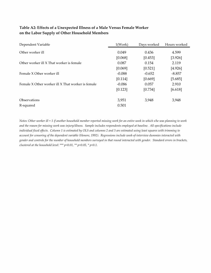
Table A2: Effects of a Unexpected Illness of a Male Versus Female Worker

on the Labor Supply of Other Household Members


Other worker ill 0.049 0.436 4.599

[0.068] [0.453] [3.926]

Other worker ill X That worker is female 0.087 0.154 2.119

[0.069] [0.521] [4.926]

Female X Other worker ill -0.088 -0.652 -8.857

[0.114] [0.669] [5.685]

Female X Other worker ill X That worker is female -0.086 0.057 2.910

[0.123] [0.734] [6.618]


R-squared 0.501


and the reason for missing work was injury/illness. Sample includes respondents employed at baseline. All specifications include

individual fixed effects. Column 1 is estimated by OLS and columns 2 and 3 are estimated using least squares with trimming to

account for censoring of the dependent variable (Honore, 1992). Regressions include week-of-interview dummies interacted with

gender and controls for the number of household members surveyed in that round interacted with gender. Standard errors in brackets,

clustered at the household level: *** p<0.01, ** p<0.05, * p<0.1.

Table A3: Effects of a Worker's Unexpected Illness on the Labor Supply of

Other Household Members Who are Not Employed at Baseline


Other worker ill -0.032 -0.372 -8.467

[0.044] [0.836] [6.298]

Other worker ill X Female 0.007 -0.668 5.603

[0.055] [1.104] [9.330]


R-squared 0.497

Notes: Other worker ill = 1 if another household member reported missing work for an entire week in which s/he

was planning to work and the reason for missing work was injury/illness. Sample includes only respondents

not employed at baseline. All specifications include individual fixed effects. Column 1 is estimated by OLS and

columns 2 and 3 are estimated using least squares with trimming to account for censoring of the dependent

variable (Honore, 1992). Regressions include week-of-interview dummies interacted with gender and controls

for the number of household members surveyed in that round interacted with gender. Standard errors in


Table A4: Effects of Future and Past Illness on Labor Supply


Panel A: Other worker ill next week

Other worker ill next week 0.013 0.173 2.423

[0.046] [0.245] [2.401]

Other worker ill next week X Female -0.006 0.357 3.413

[0.055] [0.335] [3.495]


R-squared 0.500

Panel B: The worker him/herself ill next week

Self ill next week -0.059 -0.709 -6.252

[0.092] [0.613] [4.667]

Self next week X Female -0.005 0.045 2.531

[0.116] [0.823] [6.834]


R-squared 0.508

Panel C: Other worker ill last week

Other worker ill 0.085** 0.503** 5.787**

[0.042] [0.224] [2.263]

Other worker ill X Female -0.120** -0.668** -7.277**

[0.055] [0.333] [3.051]

Other worker ill last week 0.061 0.154 1.898

[0.044] [0.245] [2.522]

Other worker ill last week X Female -0.052 -0.005 -1.742

[0.048] [0.308] [3.238]


R-squared 0.538

Panel D: Self ill last week

Other worker ill 0.097** 0.538** 6.226***

[0.044] [0.231] [2.254]

Other worker ill X Female -0.131** -0.674* -7.680**

[0.057] [0.347] [3.087]

Self ill last week 0.038 0.160 1.092

[0.117] [0.771] [5.251]

Self ill last week X Female -0.077 -0.404 -2.679

[0.130] [0.949] [7.249]


R-squared 0.536

Notes: Other worker ill = 1 in a given week if another household member reported missing work that entire week (if s/he

was planning to work that week) and the reason for missing work was injury/illness. Self ill next week/previous week = 1 if

that worker reported missing work that entire next week (if s/he was planning to work that week) and the reason for missing

work was injury/illness. Sample includes respondents employed at baseline. Regressions include individual fixed effects,

week-of-interview dummies interacted with gender and controls for the number of household members surveyed in that

round interacted with gender. Column 1 is estimated by OLS and columns 2 and 3 are estimated using least squares with

trimming to account for censoring of the dependent variable (Honore, 1992). Standard errors in brackets, clustered at the

household level.

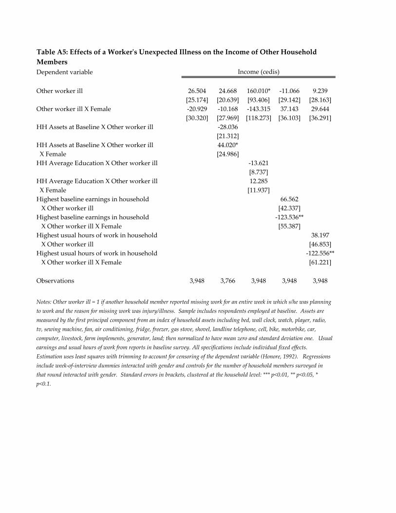
Table A5: Effects of a Worker's Unexpected Illness on the Income of Other Household

Members

Dependent variable

Other worker ill 26.504 24.668 160.010* -11.066 9.239

[25.174] [20.639] [93.406] [29.142] [28.163]

Other worker ill X Female -20.929 -10.168 -143.315 37.143 29.644

[30.320] [27.969] [118.273] [36.103] [36.291]

HH Assets at Baseline X Other worker ill -28.036

[21.312]

HH Assets at Baseline X Other worker ill 44.020*

X Female [24.986]

HH Average Education X Other worker ill -13.621

[8.737]

HH Average Education X Other worker ill 12.285

X Female [11.937]

Highest baseline earnings in household 66.562

X Other worker ill [42.337]

Highest baseline earnings in household -123.536**

X Other worker ill X Female [55.387]

Highest usual hours of work in household 38.197

X Other worker ill [46.853]

Highest usual hours of work in household -122.556**

X Other worker ill X Female [61.221]

Observations 3,948 3,766 3,948 3,948 3,948

Income (cedis)

Notes: Other worker ill = 1 if another household member reported missing work for an entire week in which s/he was planning

to work and the reason for missing work was injury/illness. Sample includes respondents employed at baseline. Assets are

measured by the first principal component from an index of household assets including bed, wall clock, watch, player, radio,

tv, sewing machine, fan, air conditioning, fridge, freezer, gas stove, shovel, landline telephone, cell, bike, motorbike, car,

computer, livestock, farm implements, generator, land; then normalized to have mean zero and standard deviation one. Usual

earnings and usual hours of work from reports in baseline survey. All specifications include individual fixed effects.

Estimation uses least squares with trimming to account for censoring of the dependent variable (Honore, 1992). Regressions

include week-of-interview dummies interacted with gender and controls for the number of household members surveyed in

that round interacted with gender. Standard errors in brackets, clustered at the household level: *** p<0.01, ** p<0.05, *

p<0.1.

Table A6: Distribution of gender and high earner/hours status within household

Male Female Total

Highest Baseline Earnings in Household

No Count 74 139 213

Percent 38.7 58.2 49.5

Yes Count 117 100 217

Percent 61.3 41.8 50.5

Total 191 239 430

100 100 100

Highest Usual Hours of Work in Household

No Count 79 124 203

Percent 41.4 51.9 47.2

Yes Count 112 115 227

Percent 58.6 48.1 52.8

Total 191 239 430

100 100 100

Highest Baseline Earnings in Household; Households with 2+ Workers Employed at Baseline only

No Count 74 137 211

Percent 51.4 69.2 61.7

Yes Count 70 61 131

Percent 48.6 30.8 38.3

Total 144 198 342

100 100 100

Highest Usual Hours of Work in Household; Households with 2+ Workers Employed at Baseline only

No Count 79 124 203

Percent 54.9 62.6 59.4

Yes Count 65 74 139

Percent 45.1 37.4 40.6

Total 144 198 342

100 100 100

Notes: Sample includes individuals employed at baseline.

Table A7: Week-to-week variation in wages

Dependent variable = Mean absolute within-person deviation in weekly hours worked

Males Females Males Females

Wage work, irregular payment 11.982 9.678 7.207 5.574

Wage work, regular payment 9.180 7.292 5.152 4.309

Self employed 10.331 8.870 6.597 6.833

P-value from F-test of difference in coefficients 0.496 0.473 0.321 0.005

Work close to home 9.792 8.224 5.854 6.249

Work far from home 7.758 5.756 7.251 6.729

P values from T-test of difference in coefficients 0.008 0.001 0.001 0.050

Including weeks with zero

hours

Conditional on any hours

worked

Notes: Sample includes respondents employed at baseline. P-values use standard errors clustered at the household level. Regular wage

work is defined as jobs for which the respondent listed frequency of pay as every week, every two weeks, or every month; any other

responses are characterized as irregular wage work.

Table A8: Heterogeneous Effects by Household Demographics

Dependent variable 1(Work)Days

worked

Hours

worked1(Work)

Days

worked

Hours

worked

Panel A: Working age adults

Other worker ill 0.147* 0.509 5.571 0.118* 0.346 3.935

[0.085] [0.416] [4.420] [0.064] [0.294] [3.168]

Other worker ill X Female -0.237* -0.404 -3.346 -0.165 -0.196 -2.369

[0.143] [0.785] [6.414] [0.102] [0.588] [4.999]

Number of Adults 18 to 64 in household -0.006 -0.001 -0.039


Number of Adults 18 to 64 in household 0.012 -0.020 -0.347


Number of Adults 18 to 64 out of LF in HH -0.005 0.076 0.670


Number of Adults 18 to 64 out of LF in HH 0.008 -0.156 -1.577


Observations 3,786 3,783 3,783 3,786 3,783 3,783

R-squared 0.51 0.51

Panel B: Older adults

Other worker ill 0.120*** 0.552** 5.607** 0.117*** 0.540** 5.800***

[0.044] [0.230] [2.184] [0.041] [0.215] [2.054]

Other worker ill X Female -0.161*** -0.604* -6.626** -0.156*** -0.565 -6.199**

[0.061] [0.365] [3.215] [0.058] [0.345] [3.054]

Number of Adults 65+ in household -0.113* -0.381 -2.437


Number of Adults 65+ in household 0.131* 0.334 4.762


Number of Adults 65+ in household out of -0.175** -0.577** -7.995***

labor market X Other worker ill [0.068] [0.245] [2.864]

Number of Adults 65+ in household out of 0.164*** -0.029 0.695

labor market X Other worker ill X Female [0.062] [0.502] [4.861]

Observations 3,786 3,783 3,783 3,786 3,783 3,783

R-squared 0.51 0.51

Table A8: Heterogeneous Effects by Household Demographics (continued)

Dependent variable 1(Work)Days

worked

Hours

worked1(Work)

Days

worked

Hours

worked

Panel C: Children

Other worker ill 0.077 0.299 4.435* 0.021 0.542 8.433

[0.054] [0.259] [2.616] [0.108] [0.627] [5.675]

Other worker ill X Female -0.161** -0.671 -8.865** -0.068 -0.892 -10.956*

[0.071] [0.437] [4.056] [0.115] [0.740] [6.477]

Number of children under 10 in household 0.032 0.207 0.857


Number of children under 10 in household 0.016 0.131 3.013


Number of own children under 10 0.060 0.096 -0.870


Number of own children under 10 -0.037 0.209 2.930


Observations 3,786 3,783 3,783 2,724 2,722 2,722

R-squared 0.511 0.53

Panel D: Marriage

Other worker ill 0.045 0.075 2.949

[0.058] [0.246] [2.489]

Other worker ill X Female -0.091 -0.326 -5.526

[0.083] [0.386] [3.540]

Other worker ill X Married 0.107 0.745* 4.104

[0.073] [0.383] [3.756]

Other worker ill X Married X Female -0.090 -0.337 -0.380

[0.103] [0.637] [5.640]


R-squared 0.508

Notes: Other worker ill = 1 if another household member reported missing work for an entire week in which they were planning to

work and the reason for missing work was injury/illness. Sample includes respondents employed at baseline. All specifications

include individual fixed effects. Column 1 is estimated by OLS and columns 2 and 3 are estimated using least squares with trimming

to account for censoring of the dependent variable (Honore, 1992). Regressions include week-of-interview dummies interacted with

gender and controls for the number of household members surveyed in that round interacted with gender. Standard errors in


labor supply responses to illness shocks: …faculty.washington.edu/rmheath/hmr.pdf1 labor supply...

Documents