laboratorio di problemi inversi esercitazione 1: il...
TRANSCRIPT

Laboratorio di Problemi InversiEsercitazione 1: il problema di image deblurring
Luca Calatroni
Dipartimento di Matematica, Universita degli studi di Genova
11 Aprile 2016.
Luca Calatroni (DIMA, Unige) Esercitazione 1, Lab. Prob. Inv. 11 Aprile 2016 1 / 23

Outline
1 Dettagli, orari ed esame
2 Part I: reading and visualising images in MATLAB
3 Part II: Forward problemStandard Fourier multiplicationMATLAB Image processing toolbox functions
4 Part III: naive inversionAdding noise
5 Part IV: Tikhonov regularisation
Luca Calatroni (DIMA, Unige) Esercitazione 1, Lab. Prob. Inv. 11 Aprile 2016 2 / 23

I miei contatti
Luca Calatroni:
I Dove sono? Al piano 0, al MIDA group.
I e-mail: [email protected]
I Telefono: 010-3536644
I Se non sono qui, sono a Camelot, in centro o a qualche confenza in giro. . .
. . . se avete bisogno contattatemi e ci organizziamo per un ricevimento
Luca Calatroni (DIMA, Unige) Esercitazione 1, Lab. Prob. Inv. 11 Aprile 2016 3 / 23

Orari
I Dove: PC1
I Quando: 11/4 (16:00-18:00), 18/4 (16:00-18:00), 28/4 (11:00-13:00),. . .
I TOT. ore: 6 (prima parte) + 4 (seconda parte) + 2 (varie)
I Tipologia esame: relazione individuale su un’esperienza di laboratorio.
In particolare, sull’esame:
- Non tutti lo stesso argomento!
- Resoconto del laboratorio scelto + commento + piccola variazione sul tema.
- Codici da inviare insieme alla relazione e loro discussione.
- Valutazione: da 0 a 3 da sommare al voto finale.
. . . domande?
Luca Calatroni (DIMA, Unige) Esercitazione 1, Lab. Prob. Inv. 11 Aprile 2016 4 / 23

Several inverse problems around us. . .
Luca Calatroni (DIMA, Unige) Esercitazione 1, Lab. Prob. Inv. 11 Aprile 2016 5 / 23

The typical inverse problem
We will consider the problem of recovering x from an observed y :
y = Ax + n
where:
I A is the matrix modelling the forward problem
I y is the measured data
I n is the noise component corrupting the data.
Deblurring problem
Since playing in 1D is cool, but boring, we will work directly on the imagedeblurring problem (very common in applications. . . ).
Luca Calatroni (DIMA, Unige) Esercitazione 1, Lab. Prob. Inv. 11 Aprile 2016 6 / 23

Outline
1 Dettagli, orari ed esame
2 Part I: reading and visualising images in MATLAB
3 Part II: Forward problemStandard Fourier multiplicationMATLAB Image processing toolbox functions
4 Part III: naive inversionAdding noise
5 Part IV: Tikhonov regularisation
Luca Calatroni (DIMA, Unige) Esercitazione 1, Lab. Prob. Inv. 11 Aprile 2016 7 / 23

Quick recap
You should find some previously loaded data in the esercitazione 1 folder.
1 We will use some available MATLAB images: use imread to read images
2 Load: ’cameraman.tif’ image and convert to double precision
3 Load also the Shepp-Logan phantom using
im1=phantom(’Modified Shepp-Logan’, 256);
4 Visualise using imshow and imagesc with appropriate colormap(gray),normalisation?
5 Load ’peppers.png’, it is a RGB image (n ×m × 3). Show different R, G,B, channels. To convert an RGB image to a grayscale image use:
im gray=double(rgb2gray(im color));
. . . try to make this as general as you can so that you can play around with it!
(- compute and store the size of the loaded images)
Luca Calatroni (DIMA, Unige) Esercitazione 1, Lab. Prob. Inv. 11 Aprile 2016 8 / 23

Quick recap
You should find some previously loaded data in the esercitazione 1 folder.
1 We will use some available MATLAB images: use imread to read images
2 Load: ’cameraman.tif’ image and convert to double precision
3 Load also the Shepp-Logan phantom using
im1=phantom(’Modified Shepp-Logan’, 256);
4 Visualise using imshow and imagesc with appropriate colormap(gray),normalisation?
5 Load ’peppers.png’, it is a RGB image (n ×m × 3). Show different R, G,B, channels.
To convert an RGB image to a grayscale image use:
im gray=double(rgb2gray(im color));
. . . try to make this as general as you can so that you can play around with it!
(- compute and store the size of the loaded images)
Luca Calatroni (DIMA, Unige) Esercitazione 1, Lab. Prob. Inv. 11 Aprile 2016 8 / 23

Quick recap
You should find some previously loaded data in the esercitazione 1 folder.
1 We will use some available MATLAB images: use imread to read images
2 Load: ’cameraman.tif’ image and convert to double precision
3 Load also the Shepp-Logan phantom using
im1=phantom(’Modified Shepp-Logan’, 256);
4 Visualise using imshow and imagesc with appropriate colormap(gray),normalisation?
5 Load ’peppers.png’, it is a RGB image (n ×m × 3). Show different R, G,B, channels. To convert an RGB image to a grayscale image use:
im gray=double(rgb2gray(im color));
. . . try to make this as general as you can so that you can play around with it!
(- compute and store the size of the loaded images)
Luca Calatroni (DIMA, Unige) Esercitazione 1, Lab. Prob. Inv. 11 Aprile 2016 8 / 23

Quick recap
You should find some previously loaded data in the esercitazione 1 folder.
1 We will use some available MATLAB images: use imread to read images
2 Load: ’cameraman.tif’ image and convert to double precision
3 Load also the Shepp-Logan phantom using
im1=phantom(’Modified Shepp-Logan’, 256);
4 Visualise using imshow and imagesc with appropriate colormap(gray),normalisation?
5 Load ’peppers.png’, it is a RGB image (n ×m × 3). Show different R, G,B, channels. To convert an RGB image to a grayscale image use:
im gray=double(rgb2gray(im color));
. . . try to make this as general as you can so that you can play around with it!
(- compute and store the size of the loaded images)
Luca Calatroni (DIMA, Unige) Esercitazione 1, Lab. Prob. Inv. 11 Aprile 2016 8 / 23

Outline
1 Dettagli, orari ed esame
2 Part I: reading and visualising images in MATLAB
3 Part II: Forward problemStandard Fourier multiplicationMATLAB Image processing toolbox functions
4 Part III: naive inversionAdding noise
5 Part IV: Tikhonov regularisation
Luca Calatroni (DIMA, Unige) Esercitazione 1, Lab. Prob. Inv. 11 Aprile 2016 9 / 23

Outline
1 Dettagli, orari ed esame
2 Part I: reading and visualising images in MATLAB
3 Part II: Forward problemStandard Fourier multiplicationMATLAB Image processing toolbox functions
4 Part III: naive inversionAdding noise
5 Part IV: Tikhonov regularisation
Luca Calatroni (DIMA, Unige) Esercitazione 1, Lab. Prob. Inv. 11 Aprile 2016 10 / 23

How to create blur?
For the moment let us think at the problem with no noise and in a matricial form:
Y = A ∗ X , X ,Y ∈ Rn×m,
where ∗ stands for the convolution operation (deblurring problem).How to model the blur problem?
1 read the ’motion h.png’ image you find in the folder + normalise it;
2 visualise it: this will generate horizontal motion blur in the image. How youwill create a vertical motion blur kernel?
3 Using MATLAB functions: fft2, ifft2, fftshift and recalling that
Y = A ∗ X ⇔ Y = AX
in the Fourier domain, compute the blurred (horizontal and vertical) versionsof the cameraman image.
4 Remember to shift!
Luca Calatroni (DIMA, Unige) Esercitazione 1, Lab. Prob. Inv. 11 Aprile 2016 11 / 23

Outline
1 Dettagli, orari ed esame
2 Part I: reading and visualising images in MATLAB
3 Part II: Forward problemStandard Fourier multiplicationMATLAB Image processing toolbox functions
4 Part III: naive inversionAdding noise
5 Part IV: Tikhonov regularisation
Luca Calatroni (DIMA, Unige) Esercitazione 1, Lab. Prob. Inv. 11 Aprile 2016 12 / 23

Creating blur filters using MATLAB
MATLAB offers a variety of realistic blur kernels you can use to artificially bluryour image.
fspecial(’type’, parameters)
’motion’: horizontal motion, vertical motion, generic motion,’gaussian’: gaussian blur.
I Supported by the use of MATLAB help, create horizontal, vertical andgeneric motion (shift=15, inclination 30) and Gaussian kernel (dimension =[21 21], σ2 = 3).
I Visualise generic motion and Gaussian one: comment on their size.
I Blur the image with the built blurs using the function imfilter(image,
PSF). Show the result.
Luca Calatroni (DIMA, Unige) Esercitazione 1, Lab. Prob. Inv. 11 Aprile 2016 13 / 23
Outline
1 Dettagli, orari ed esame
2 Part I: reading and visualising images in MATLAB
3 Part II: Forward problemStandard Fourier multiplicationMATLAB Image processing toolbox functions
4 Part III: naive inversionAdding noise
5 Part IV: Tikhonov regularisation
Luca Calatroni (DIMA, Unige) Esercitazione 1, Lab. Prob. Inv. 11 Aprile 2016 14 / 23

Let’s invert!
Use Shepp-Logan image.
I Compute Gaussian PSF of the same images size.
I To invert use the same idea as before: take the real part of
F−1 (F(Y )/F(PSF )) ,
what do we observe?
I Stupid test: try to blur the image as
ifft2(((fft2(image).*fft2(PSF))./(fft2(PSF))).
We are multiplying and dividing by the same quantity, but still. . .
I Try to add some small regularisation at the denominator. . . what do youobserve?
Filtering
The idea is to remove small frequencies by either regularisation or thresholding. . .
Luca Calatroni (DIMA, Unige) Esercitazione 1, Lab. Prob. Inv. 11 Aprile 2016 15 / 23

How to avoid that?
Again using Shepp-Logan (synthetic image).
I psf2otf(PSF,size(image)) maps the PSF window into the Fourier domainand adapts to the desired size of the image + filtering (small frequencies areset equal to 1).
I Now invert!
I Show the results. It looks we managed!
I . . . just to double-check: let’s do one similar test (or all, as you like) for thecameraman image. What do you observe?
Luca Calatroni (DIMA, Unige) Esercitazione 1, Lab. Prob. Inv. 11 Aprile 2016 16 / 23

Why is this happening?
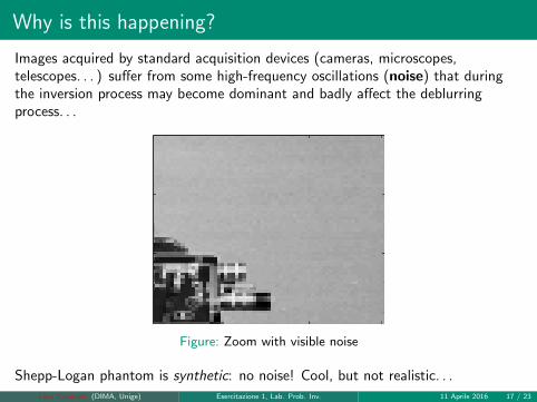
Images acquired by standard acquisition devices (cameras, microscopes,telescopes. . . ) suffer from some high-frequency oscillations (noise) that duringthe inversion process may become dominant and badly affect the deblurringprocess. . .
Figure: Zoom with visible noise
Shepp-Logan phantom is synthetic: no noise! Cool, but not realistic. . .
Luca Calatroni (DIMA, Unige) Esercitazione 1, Lab. Prob. Inv. 11 Aprile 2016 17 / 23
Why is this happening?
Images acquired by standard acquisition devices (cameras, microscopes,telescopes. . . ) suffer from some high-frequency oscillations (noise) that duringthe inversion process may become dominant and badly affect the deblurringprocess. . .
Figure: Zoom with visible noise
Shepp-Logan phantom is synthetic: no noise! Cool, but not realistic. . .
Luca Calatroni (DIMA, Unige) Esercitazione 1, Lab. Prob. Inv. 11 Aprile 2016 17 / 23
Outline
1 Dettagli, orari ed esame
2 Part I: reading and visualising images in MATLAB
3 Part II: Forward problemStandard Fourier multiplicationMATLAB Image processing toolbox functions
4 Part III: naive inversionAdding noise
5 Part IV: Tikhonov regularisation
Luca Calatroni (DIMA, Unige) Esercitazione 1, Lab. Prob. Inv. 11 Aprile 2016 18 / 23

Creating noisy measurements
Recall:
Y = A ∗ X + N
I Use randn(size(image)) to generate a normalised Gaussian-distributednoise component. Multiply by
√σ2 = 0.005.
I Create noisy version of blurred Shepp-Logan data, visualise it (use Gaussianblurred version only).
I Check that the same inversion problem is also happening now.
→ Introducing threshold for small values of |OTF |Use find to find the indices where |OTF | < thresh and replace the matrix therewith 1.
I Is the result getting any better?
Luca Calatroni (DIMA, Unige) Esercitazione 1, Lab. Prob. Inv. 11 Aprile 2016 19 / 23

Outline
1 Dettagli, orari ed esame
2 Part I: reading and visualising images in MATLAB
3 Part II: Forward problemStandard Fourier multiplicationMATLAB Image processing toolbox functions
4 Part III: naive inversionAdding noise
5 Part IV: Tikhonov regularisation
Luca Calatroni (DIMA, Unige) Esercitazione 1, Lab. Prob. Inv. 11 Aprile 2016 20 / 23

Formulation as a linear inverse problem
By vectorisation of X ,N and, consequently Y and the linearity of theconvolution operation, the problem can be formulated as:
y = Ax + n, x , n, y ∈ Rnm×1,A ∈ Rnm×nm.
The construction of the matrix A deserves some attention (depends on theboundary conditions considered, the PSF used. . . ).
I Reduce the size of the problem: use imresize to the phantom image to geta new image of size [100 100], then blur (Gaussian, size PSF = 5, σ2 = 3)and add noise with σ2 = 1e − 4.
I Load the A matrix in ’blur matrix.mat’ (760 MB!!).
I So now we have a linear inverse problem: what happens when you simply usethe MATLAB backslash and invert?
Luca Calatroni (DIMA, Unige) Esercitazione 1, Lab. Prob. Inv. 11 Aprile 2016 21 / 23

Tikhonov regularisation
Tikhonov regularisation makes the inversion feasible! It solves
minx‖Ax − y‖2 + λ‖x‖2, λ > 0.
Fix λ = 0.1.
Using Euler:
AT (Ax − y) + λx = 0 ⇔ x = (ATA + λ Id)−1(AT y)
. . . slow. . .
Luca Calatroni (DIMA, Unige) Esercitazione 1, Lab. Prob. Inv. 11 Aprile 2016 22 / 23

Tikhonov regularisation
Tikhonov regularisation makes the inversion feasible! It solves
minx‖Ax − y‖2 + λ‖x‖2, λ > 0.
Fix λ = 0.1.
Using Euler:
AT (Ax − y) + λx = 0 ⇔ x = (ATA + λ Id)−1(AT y)
. . . slow. . .
Luca Calatroni (DIMA, Unige) Esercitazione 1, Lab. Prob. Inv. 11 Aprile 2016 22 / 23

Alternative (no computation of A′)
I Recalling that for vector w , z
‖w‖2 + ‖z‖2 = wTw + zT z =
[yz
]T [yz
]=
∥∥∥∥[yz]∥∥∥∥2
2
write an equivalent formulation of Tikhonov regularisation (much moreefficient numerically!).
I Solve
minx
∥∥∥∥[ Ax −yλ Id x 0
]∥∥∥∥2
2
I Invert and show the result for different choices of λ.
Luca Calatroni (DIMA, Unige) Esercitazione 1, Lab. Prob. Inv. 11 Aprile 2016 23 / 23