laboratory and numerical investigation of interface ... reinforced concr… · laboratory and...

Laboratory and Numerical Investigation of Interface Debonding

of Thin and Ultrathin Bonded Concrete Overlays of Asphalt

Pavements and Its Effect on the Critical Stress of the Overlay

1. INTRODUCTION

One of the most significant differences in designing bonded concrete overlays of asphalt

pavements (BCOA) as compared to conventional concrete overlays is to ensure the

presence of the interface bond between the overlay and the underlying hot mixed asphalt

(HMA). An effective bond reduces the tensile stress in the overlay making it possible for

BCOA to carry the design traffic. Vandenbossche and Fagerness (2002) identified three

general modes for the failure of the bond, namely debonding at the interface,

delamination between HMA lifts, and HMA raveling. All three modes reduce the

composite stiffness of the BCOA structure resulting in the accelerated cracking of the

overlay. HMA raveling is more of a material and moisture-related problem. It might

rarely occur for HMA that is appropriately designed and also kept from moisture. The

other two modes of deterioration occur more frequently. For example, Chabot et al.

(2008) also observed interface debonding and HMA cracking in their accelerated loading

tests.

The development of interface debonding is not completely understood. Previous research

only qualitatively indicates that the interface debonding develops due to repetitive traffic

and environmental loading (Pouteau et al., 2004, Chabot et al., 2008) and the rate of the

development depends on the surface preparation (Delatte and Sehdev, 2003), and

temperature and moisture (Al-Qadi et al. 2008). However, no quantitative study has been

conducted in order to incorporate interface debonding into design. As a result, a constant

adjustment factor has been accepted in design to account for the increase of the stress in

the overlay due to partial bonding. Tarr et al. (1998) proposed 50%-60% for the increase

of the stress, based on the comparison between predicted and measured strains from three

projects in Colorado. Wu et al. (1999) suggested a stress increase of 20%-60% based on

three projects, one in Missouri and two in Colorado. The use of such a constant stress

adjustment factor might lead to very unreliable designs, since the calibration projects

used only represents a few design scenarios and more importantly the interface

debonding develops gradually and does not remain constant.

Interface debonding occurs when the facture energy release rate exceeds a critical value.

The failure can be further broken down into Mode I (tensile) and Mode II (shear)

depending on the nature of the stress contributing to the fracture at the interface, as

shown in Figure 1.

Figure 1 Two common modes of interface debonding

The Mode I debonding stress can be found at the interface from the unloaded side of a

joint when the other side of the joint is loaded by a traveling wheel. Differential

deflection across the joint might be significant for thin and ultrathin whitetopping

considering that the small cross section of the joints provides little aggregate interlock

and it will tend to peel off the asphalt from the concrete overlay. The Mode I debonding

stress can also develop due to the curling/warping of the overlay slabs due to

temperature/moisture gradients (Kim and Nelson, 2004). When the slabs curl/warp up,

the continuous asphalt tends to stay flat and thus induces debonding at the PCC/HMA

interface. With respect to Mode II shear failure, the differential length change between

the PCC and HMA induces shear stress that can damage the interface bond (Granju,

2004). The braking action of the wheel when approaching pavement intersections can

also lead to shear failure.

It is unlikely that either of the abovementioned modes for interface debonding should be

caused by a single pass of vehicular load, but rather by fatigue. Therefore, the objective

of this study is to gain a better understanding of the development of interface debonding

due to fatigue loading and then incorporate it into the design of BCOA. Due to the

limitation in cost and time, only Mode I interface debonding was studied, which is

believed to be the dominant mode.

It is well known that Paris’ law, Equation (1), could be used to define fractures due to

fatigue. Therefore, the growth of the debonded area in Equation (2) can be established

based on Paris’s law.

(

)

(1)

where is the growth of the debonded area; is the number of the applied loads;

and are scaling constants; is the transient energy release rate due to the fatigue

loads and is the critical energy release rate at which the interface crack will propagate.

As the first step of this study, the critical fracture energy release rate in Mode I was

established for whitetopping specimens. Various factors were considered in terms of

their effect on the critical fracture energy release rate, such as the preparation of asphalt

surfaces (milled vs. unmilled), temperature and moisture. The results for this step are

summarized in Chapter 2.

A finite element model was developed as the second step to calculate the transient energy

release rate. Cohesive elements were first calibrated using the specimen tested in the first

step and then used in the finite element model for whitetopping slabs. The results for this

step are summarized in Chapter 3.

In the third step, accelerated loading testing (ALT) was carried out to study the

development of interface debonding due to fatigue loading. The empirical constants in

Equation (1) were calibrated based on ALT results. Two types of surface preparation for

asphalt were used to study their effects on the interface debonding. During this step, the

debonded area was determined by two nondestructive methods. The first method is based

on the impact echo principles and the other method is based on the comparison between

the measured and the predicted deflections of the whitetopping slabs. The results for this

step are summarized in Chapter 4.

In the last step, the effect of interface debonding on the critical stress in the overlay is

investigated. It is proposed in this study that the degree of debonding should be

characterized by the area of debonding relative to the area of the overlay slab,

i.e. ⁄ ⁄ in Figure 1.

Figure 2. Definition of degree of interface debonding.

The critical stress in the overlay should increase as the degree of debonding increases, i.e.

Equation (2).

(2)

where is the increase of critical stress in the overlay; is the degree of debonding

that equals to ⁄ ⁄ ; and are the debonded area and the area of the slab,

respectively. The results for this step are summarized in Chapter 5.

A

B

2. MODE-I CRITICAL ENERGY RELEASE RATE

In this chapter, the critical fracture energy release rate was characterized for two types of

interface, in terms of the milling of the asphalt. It was first noted in the test sections

constructed in Iowa that milling the HMA prior to the placement of the overlay

contributed to higher bond strengths between the HMA and the overlay. Milling the

HMA created a macrotexture that resulted in a higher bond strength, as measured using

the Iowa shear test. The results from a study (Tarr et al., 1998) funded by the Colorado

Department of Transportation provided similar results. In the study, strain measurements

were made on in-service pavements. It was found that the dynamic strains measured for

overlays placed on milled HMA were 25% lower than for unmilled HMA surfaces.

Chabot et al. (2008) also found a much rougher failure surface for debonded interfaces

when HMA was shot blasted prior to the overlay to increase the texture. In the research,

whitetopping slabs were loaded by a test track and the coring results indicated that it was

tougher to fracture an interface with increased texture.

A description of the test procedure and test specimens developed to characterize the

Mode I failure at the PCC/HMA interface will be first provided followed by the

presentation of test results. Then, an analytical model that was used to process the

experimental data will be introduced. Finally, the model will be validated using the test

results.

2.1 Wedge Splitting Test

2.1.1 Test configuration

The shape of the specimens used in the wedge splitting test (WST) is illustrated in Figure

3. A WST specimen is made of half PCC and half HMA, with a notch sawed at the

interface to guarantee the initiation of the crack at the desired location, i.e. the interface.

A steel cap with two round bearings (one at the front and the other at the back) is placed

on top of each half, which is responsible for transforming the external axial load to

horizontal splitting forces through a wedge. The bearings are managed to align with the

gravity centers of the corresponding half specimen. The WST specimen rests on two

linear supports, which are aligned with the bearings. These alignments minimize the

effect of vertical force on the fracture of the interface.

A clip gage is instrumented to the end of the starter notch to monitor the crack mouth

opening displacement (CMOD), as shown in Figure 4. Besides the starter notch, guide

notches that are usually 1/5 to 1/4 in deep are also sawed on both sides of the specimen to

ensure that the interfacial crack propagates along the interface. After the instrumentation,

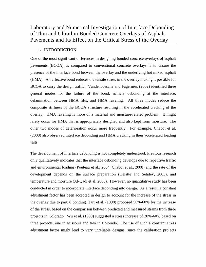
a wedge is placed between the bearings and the whole assembly is placed under an

actuator for axial loading, as shown in Figure 5.

Figure 3 Sketch of wedge splitting test configuration

Figure 4 WST specimen instrumented with clip gage for CMOD and load caps.

HMA PCC

Linear support

a1

b1

d1

e1

f1

g1

4mm

Starter notch 1

A1

G1

E1

F1B1

D1

Clip gage for CMOD

Load Caps

Linear support

Starter notch

Guide notch

The loading process consists of two steps. First, a sitting load of about 5-10 lbf is applied

to ensure the contact between the loading plate and the wedge when both the clip gage

and the load cell are zeroed. Second, the WST specimen is loaded to failure or a point

when the axial load decreases back to zero after peak load, with a constant rate of

CMOD. In this step, the axial load as well as the CMOD is recorded at 100 Hz for future

analysis.

Figure 5 WST specimen subjected to actuator loading.

2.1.2 Specimen preparation

The shape of the HMA half of a typical WST specimen is shown in Figure 6. It is

prepared using the following procedure. First, HMA blocks of 6-in (Length) ×6-in

(Width) ×3.5~4.5-in (Thickness) were cut from HMA slabs that were obtained from an

aged HMA surfaced road. Therefore, the thickness of the HMA halves is limited by the

thickness of the slabs, which is about 3.5 in for milled slabs and 4.5 in for unmilled slabs.

Second, one of surface corners was cut off to leave a 6-in ×1.5-in ×1-in space to

accommodate the loading cap as well as the clip gage. At last, since the WST specimen

will stay in the curing room for 28 days after casting, the HMA halves were wrapped

Actuator

Load cell

Load wedge

with duct tape to minimize the degradation of the HMA due to moisture, as shown in

Figure 7.

Figure 6 Shape of the HMA specimen before concrete casting.

Figure 7 HMA half of the WST specimen after duct tape wrapping.

After casting and curing concrete for at least 28 days, the WST specimen needs further

cuts to refine its geometry. The requirement on the geometry is strict so that a successful

test can be guaranteed. One of the most important requirements is that the corresponding

horizontal planes from the two halves are leveled. This is to guarantee the levelness of

clip gage, the bearings and linear supports so that the readings for the axial load and the

CMOD are accurate. Although it is extremely difficult to cut precisely with a 1/8-in

diamond blade, the inclination of all the horizontal planes were controlled to be less than

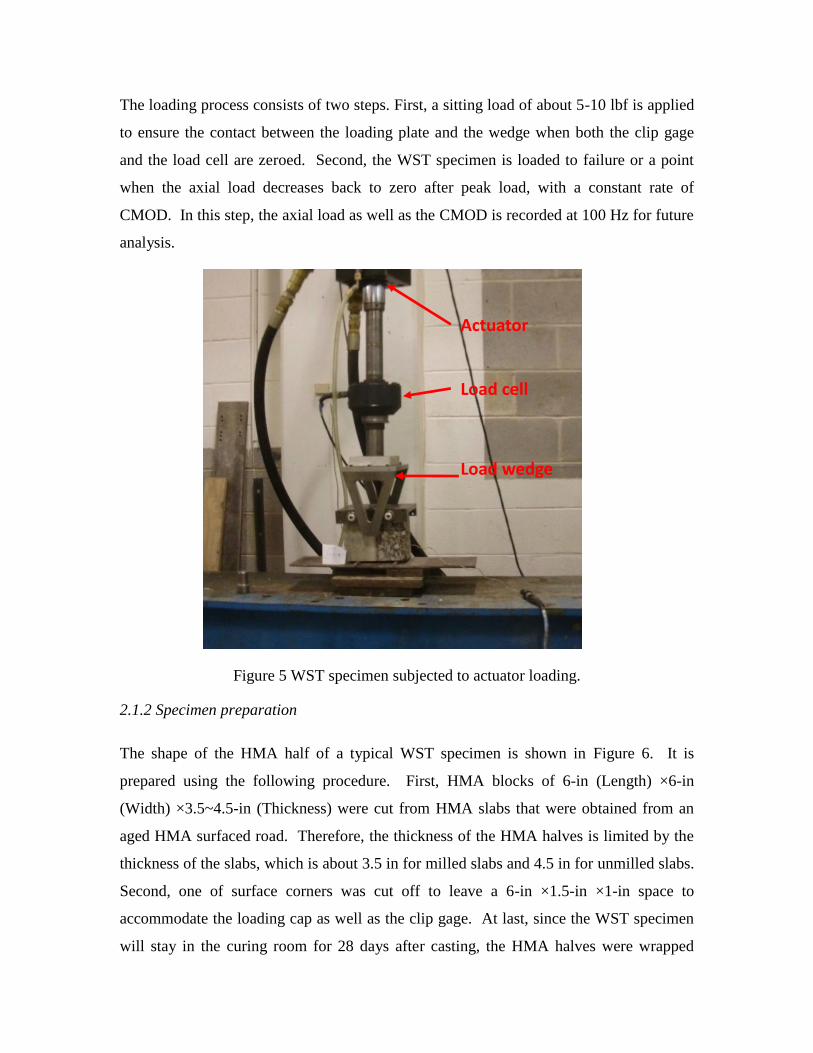
1 degree. The dimensions of the as-built specimens are measured and presented in Table

1 and Table 2. The meaning for the variables in the tables can be found in Figure 3.

Subscripts 1 and 2 represent front and back side of the WST specimens.

The WST specimens were made in two batches, namely the WST-2 batch and the WST-S

batch. Among these two batches of specimens, various notch depths were made to study

the effect of crack depth on the interface fracture property.

Another variable among the specimens is the surface condition. Sand patch test (ASTM-

E965-96, 2006) was carried out on both milled and unmilled HMA specimens to obtain a

characteristic depth, i.e. the surface roughness. The surface roughness for all the

specimens are presented in Table 1 and Table 2, where a larger number represents a

rougher surface and vice versa. Pictures have also been taken to visually record the

roughness of the HMA surfaces, which are shown from Figure 8 to Figure 11. In Figure

9 and Figure 10, the term ‘milling direction’ represents the angle between the direction of

the milling grooves and the direction of the crack propagation.

Two kinds of special specimens were made to study the effect of moisture and

temperature on the interface fracture properties. All of the specimens were cured with

duct tape wrapping and were air dried under room temperature for several days before

testing. Therefore, the wet WST specimens were made by sending them back into the

curing room with the HMA totally exposed to moisture to achieve saturation at the

interface. Some other dry specimens were stored in a freezer for a certain time to create

frozen specimens. These special specimens are also marked in Table 1 and Table 2.

Table 1. Dimensions and conditions for the WST specimens with milled HMA.

Specimen WST-

2-07

WST-

2-08

WST-

2-09

WST-

2-12

WST-

2-13

WST-

2-15

WST-

S-01

WST-

S-4

WST-

2-10

WST-

2-11

WST-

2-14

Casting date 11/23/2

011

11/23/2

011

11/23/2

011

11/23/2

011

11/23/2

011

11/23/2

011

12/12/2

011

12/12/2

011

11/23/2

011

11/23/2

011

11/23/2

011

Testing date 12/21/2

011

12/21/2

011

12/21/2

011

12/21/2

011

12/22/2

011

12/22/2

011

5/23/20

12

6/18/20

12

5/27/20

12

5/27/20

12

5/27/20

12

Weight, lbs 17.81 17.71 18.05 13.95 17.45 14.63 11.55 13.01 17.86 17.82 14.21

Dimensio

n, in

a1 3.42 3.22 3.34 2.62 2.81 2.67 2.62 2.69 3.00 3.34 2.81

a2 3.30 3.25 3.16 2.51 2.59 2.57 2.66 2.73 3.27 3.20 2.57

A1 3.55 3.92 3.82 3.12 4.20 3.06 2.34 2.96 4.04 3.73 2.96

A2 3.65 3.91 3.95 3.19 4.47 3.12 2.24 2.88 3.83 3.86 3.15

b1 2.37 2.41 2.38 1.68 1.74 1.83 1.59 1.65 2.23 2.26 1.77

b2 2.19 2.28 2.12 1.73 1.53 1.69 1.63 1.58 2.25 2.26 1.56

B1 2.66 2.65 2.77 1.78 2.97 1.98 1.25 1.93 2.80 2.73 1.94

B2 2.79 2.83 2.94 1.79 3.21 1.99 1.22 1.94 2.80 2.66 2.08

d1 5.59 5.74 5.74 5.77 5.78 5.78 5.55 5.66 5.79 5.75 5.74

d2 5.68 5.78 5.78 5.76 5.78 5.79 5.51 5.63 5.82 5.70 5.77

D1 5.68 5.82 5.81 5.73 5.69 5.87 5.56 5.70 5.72 5.83 5.81

D2 5.67 5.75 5.81 5.71 5.70 5.92 5.50 5.70 5.71 5.74 5.83

e1 1.07 0.95 1.09 1.13 1.07 0.90 0.97 1.20 0.86 1.11 1.13

e2 1.14 1.01 0.98 1.00 1.22 1.10 1.06 1.36 1.15 1.04 1.13

E1 0.98 1.10 1.02 1.07 1.14 1.25 1.14 0.96 1.14 1.01 1.12

E2 0.89 1.01 1.10 1.19 1.00 1.16 1.07 0.82 0.90 1.14 1.09

f1 1.76 1.91 1.93 1.87 1.93 1.91 1.87 1.99 1.87 1.95 1.90

f2 1.78 1.87 1.91 1.86 1.93 1.87 1.90 2.00 1.90 1.87 1.91

F1 1.71 1.85 1.88 1.73 1.91 1.90 1.93 1.99 1.96 1.89 1.84

F2 1.84 1.84 1.92 1.82 1.97 1.96 1.93 2.04 1.91 1.92 1.93

g1 3.89 3.87 3.86 3.95 3.85 3.93 3.51 3.56 3.88 3.83 3.89

g2 3.79 3.89 3.88 3.88 3.84 3.93 3.76 3.74 3.87 3.89 3.87

h1 5.82 5.64 5.74 5.68 5.82 5.79 5.85 5.60 5.74 5.79 5.73

h2 5.80 5.69 5.78 5.74 5.77 5.79 5.88 5.61 5.73 5.78 5.71

H1 5.81 5.61 5.73 5.69 5.73 5.77 5.89 5.56 5.71 5.67 5.72

H2 5.79 5.61 5.68 5.78 5.69 5.78 5.97 5.65 5.63 5.67 5.74

Starter

notch 1 0.31 0.37 0.37 0.64 0.63 0.47 0.64 0.66 0.35 0.36 0.55

Starter

notch 2 0.42 0.39 0.42 0.66 0.68 0.43 0.80 0.78 0.40 0.38 0.55

Guide

notch 1 0.20 0.23 0.22 0.23 0.36 0.23 0.15 0.17 0.25 0.23 0.21

Guide

notch 2 0.20 0.21 0.25 0.23 0.22 0.20 0.17 0.14 0.26 0.20 0.21

Milling Y Y Y Y Y Y Y Y Y Y Y

Milling direction 0 0 0 0 90 45° 0 0 0 0 0

Roughness, mil 38 68 58 68 83 79 74 68 60 65 85

Curing/tesiting

condition Dry Dry Dry Dry Dry Dry Dry Wet Frozen Frozen Frozen

Loading rate, mil/min 20 20 20 20 20 20 20 20 2 13 2

Table 2. Dimensions and conditions for the WST specimens with unmilled HMA.

Specimen WST-

2-01

WST-

2-02

WST-

2-03

WST-

S-10

WST-

S-11

WST-

S-13

WST-

S-15

WST-

S-12

WST-

S-14

WST-

2-04

WST-

2-05

WST-

2-06

Casting date 11/23/

2011

11/23/

2011

11/23/

2011

12/12/

2011

12/12/

2011

12/12/

2011

12/12/

2011

12/12/

2011

12/12/

2011

11/23/

2011

11/23/

2011

11/23/

2011

Testing date 12/21/

2011

12/22/

2011

12/22/

2011

5/23/2

012

5/23/2

012

5/23/2

012

5/23/2

012

6/18/2

012

6/18/2

012

5/27/2

012

5/27/2

012

5/27/2

012

Weight, lbs 20.99 20.22 20.86 13.13 17.79 16.04 16.46 17.44 14.92 14.92 19.36 19.17

Dimensi

on, in

a1 3.82 3.83 3.84 3.25 3.93 3.94 3.69 3.96 2.99 3.69 3.84 3.79

a2 3.85 3.90 3.89 3.19 3.94 3.83 3.64 3.92 3.00 3.75 3.87 3.79

A1 4.34 4.17 4.30 2.76 3.36 3.34 3.37 3.32 2.99 4.09 4.05 3.99

A2 4.33 4.16 4.18 2.74 3.34 3.38 3.45 3.33 2.99 4.21 4.02 3.94

b1 2.47 2.42 2.72 2.01 2.80 2.64 2.44 2.51 1.91 2.70 2.71 2.76

b2 2.47 2.47 2.69 2.01 2.86 2.62 2.56 2.57 1.92 2.72 2.78 2.67

B1 3.16 2.85 3.21 1.70 2.49 2.53 2.41 2.39 1.84 3.09 3.17 2.92

B2 3.33 2.95 3.17 1.70 2.42 2.62 2.39 2.38 1.92 3.30 3.17 2.97

d1 5.97 5.86 5.86 5.52 5.52 5.85 5.48 5.57 5.91 5.95 8.74 5.90

d2 5.94 5.82 5.82 5.68 5.52 5.95 5.50 5.71 5.89 5.97 5.65 5.94

D1 6.00 5.87 5.91 5.61 5.53 5.87 5.54 5.62 5.99 5.95 5.77 5.90

D2 6.07 5.85 5.79 5.69 5.54 6.05 5.57 5.73 5.96 5.99 5.66 5.95

e1 1.35 1.31 1.04 1.20 1.21 1.36 1.18 1.49 1.15 1.05 1.01 1.24

e2 1.43 1.38 1.14 1.25 1.19 1.37 1.02 1.29 1.19 1.15 1.15 1.16

E1 1.13 1.34 1.03 1.11 0.93 0.98 1.08 0.98 1.13 0.94 0.95 1.06

E2 1.11 1.25 0.98 1.01 0.92 0.92 1.12 1.05 1.07 0.85 0.88 0.97

f1 2.14 2.06 2.08 1.84 1.85 1.75 1.75 1.85 1.93 2.03 2.09 2.07

f2 1.99 2.06 2.03 1.83 1.86 1.85 1.77 1.94 1.93 1.97 2.01 2.10

F1 2.06 2.02 2.07 1.90 1.88 1.77 1.75 1.95 1.99 2.01 2.10 2.03

F2 1.99 2.04 2.02 1.88 1.88 1.92 1.82 1.92 1.97 2.06 2.14 2.15

g1 3.89 3.84 3.77 3.68 3.67 4.15 3.78 3.66 3.91 4.53 3.67 3.82

g2 3.95 3.79 3.76 3.85 3.63 4.05 3.73 3.74 4.04 3.88 3.63 3.73

h1 5.67 5.83 5.84 5.33 5.79 4.89 5.66 5.69 5.60 5.59 5.66 5.57

h2 5.71 5.85 5.89 5.26 5.83 4.85 5.68 5.81 5.76 5.64 5.77 5.56

H1 5.72 5.73 5.80 5.49 5.79 4.92 5.78 5.65 5.64 5.66 5.77 5.66

H2 5.74 5.74 5.77 5.45 5.84 4.90 5.77 5.77 5.75 5.62 5.86 5.61

Starter

notch 1 0.56 0.34 0.39 0.63 0.49 1.16 1.72 0.53 0.56 0.56 0.61 0.66

Starter

notch 2 0.52 0.41 0.37 0.77 0.43 1.08 1.64 0.55 0.57 0.53 0.62 0.53

Guide

notch 1 0.27 0.20 0.20 0.15 0.15 0.18 0.14 0.15 0.15 0.14 0.20 0.15

Guide

notch 2 0.26 0.21 0.18 0.15 0.15 0.14 0.16 0.16 0.17 0.17 0.15 0.15

Milling N N N N N N N N N N N N

Milling direction N/A N/A N/A N/A N/A N/A N/A N/A N/A N/A N/A N/A

Roughness, mil 19 23 22 33 31 33 30 35 25 33 22 22

Curing/tesiting

condition Dry Dry Dry Dry Dry Dry Dry Wet Wet Forzen Forzen Forzen

Loading rate,

mil/min 20 20 20 20 20 20 20 20 20 16 15 1.1

14

Figure 8 Conditions of the HMA surfaces for WST-2-01 to WST-2-06.

15

Figure 9 Conditions of the HMA surfaces for WST-2-07 to WST-2-14.

16

Figure 10 Conditions of the HMA surfaces for WST-2-15, WST-S-01 and WST-S-04.

17

Figure 11 Conditions of the HMA surfaces for WST-S-10 to WST-S-15.

18

2.2 Material Properties

2.2.1 PCC properties

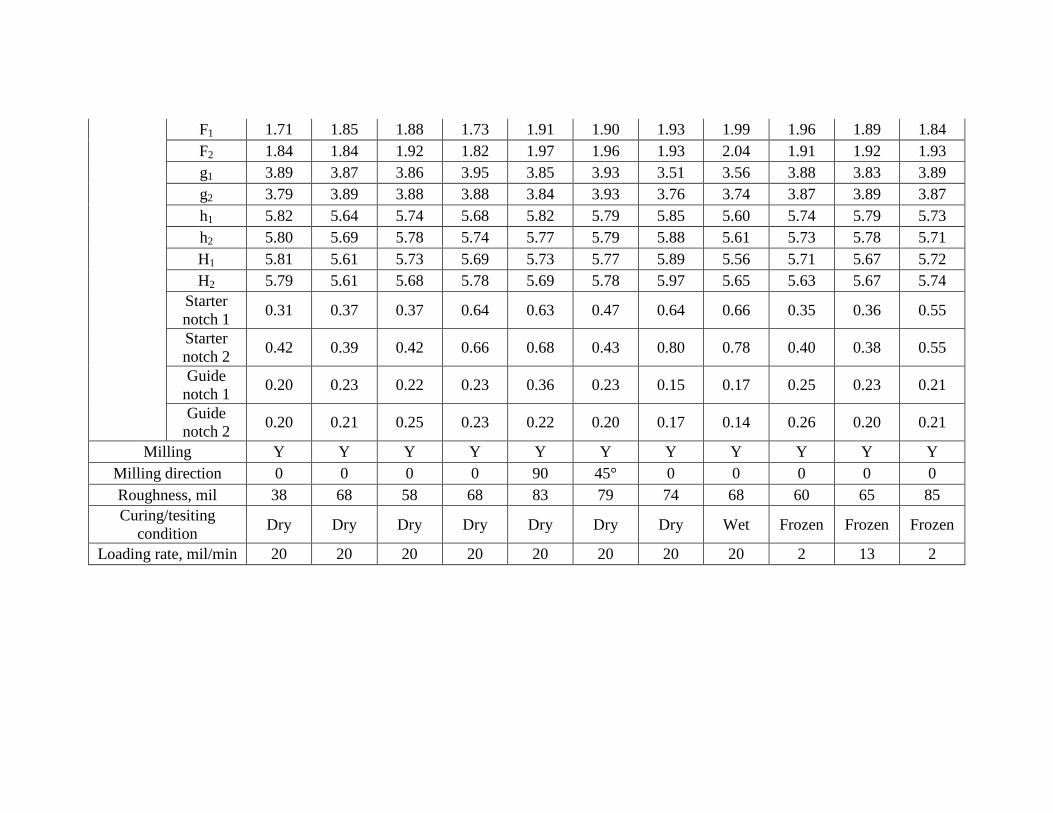
The PCC properties, i.e. compressive strength and elastic modulus, were tested for both

concrete batches of WST specimens to accompany the WST testing. The results are

presented in Table 3.

Table 3. PCC material properties.

Specimen 1 Specimen 2 Specimen 3 Average

Elastic modulus, 106 psi

WST-2 N/A 4.13 4.08 4.1

WST-S N/A 4.02 3.75 3.9

Poisson's ratio WST-2 N/A 0.21 0.2 0.21

WST-S N/A 0.2 0.18 0.19

Compressive strength, psi WST-2 4150 4000 4050 4070

WST-S 3700 3600 2700 3330

Days between casting

and testing

WST-2 28 28 28 28

WST-S 161 161 161 161

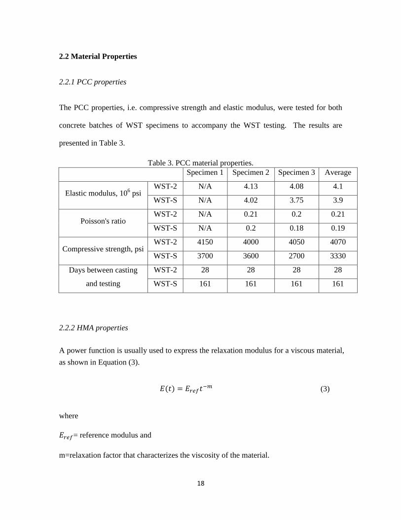
2.2.2 HMA properties

A power function is usually used to express the relaxation modulus for a viscous material,

as shown in Equation (3).

(3)

where

= reference modulus and

m=relaxation factor that characterizes the viscosity of the material.

19

For an elastic material, m in Equation (3) should be zero. For the HMA mix used in this

study, dynamic modulus was measured as shown in Table 4. The relaxation modulus was

then converted from the dynamic modulus using the approximation method proposed by

Schapery and Park (1999). The relaxation modulus determined based on the dynamic

modulus are presented in Figure 12, which were then used to calibrate the coefficients in

the power law. It was found that 250,000 psi and 0.22 for and m, respectively, result

in the best agreement between the predicted relaxation modulus by the power law and the

relaxation modulus converted from the dynamic modulus, as can be seen in Figure 12.

Table 4-Dynamic modulus for the HMA.

Temperature, °C 5 21 40

Frequency, Hz |E*|, 106psi

Phase

angle,

degree

|E*|, 106psi

Phase

angle,

degree

|E*|, 106psi

Phase

angle,

degree

10 1.535 9.5 0.83 18.3 0.23 27.7

1 1.206 12.4 0.505 23.9 0.116 27.1

0.1 0.905 16.1 0.289 26.7 0.068 25.1

0.01 0.047 23.9

Figure 12 Relaxation modulus converted based on dynamic modulus and predicted by the

power law.

0

1

2

3

4

5

6

7

-5 -4 -3 -2 -1 0 1 2 3 4 5

log

(Rel

axati

on

mod

ulu

s), m

illi

on

psi

log(Reduced time), sec

Converted from dynamic modulus Predicted using power law

20

2.3Mode-I Test Results and Analysis

2.3.1 Model development

Figure 13 shows that the WST configuration resembles the bending of two cantilever

beams. Therefore, the CMOD monitored by the clip gage can be calculated by solving

the total bending of both halves of the WST specimen subjected to the splitting force.

However, one should also note the primary difference between the two systems: a

cantilever beam has a constant length, while the crack depth in WST is a variable that

increases as the crack advances

The deflection at the end of a cantilever beam is related to the load or moment at the

same end using Equation (4).

(4)

where

=CMOD, in

=concentrated load at the end of the cantilever beam, lbf,

=moment at the end of the cantilever beam, lbf·in,

=length of the cantilever beam, in,

=stiffness of the cantilever beam, psi and

=moment of inertia of the cantilever beam, in4.

21

Figure 13 Analogy between WST and cantilever beams.

For either of the two cantilever beams in Figure 13, the deflection at its end can be

calculated using Equation (5).

(5)

where

=distance between the bearing and the notch mouth as shown in Figure 13, in.

For the HMA side of the WST, due to the viscoelasticity of the HMA, Equation (5)

becomes Equation (6).

HMA

PCC

a

Δ

F(t)

F(t)

F(t)×f

f

End of the cantilever beams

22

∫

(6)

where

=crack length as a function of time, in,

=moment of inertia of the HMA, in4.

=relaxation modulus of the HMA, psi and

=CMOD due to the deformation of the HMA half of the WST specimen.

For the PCC side of the WST, Equation (5) becomes Equation (7) considering the

elasticity of the PCC.

(7)

where

=Young’s modulus of the PCC, psi and

= moment of inertia of the PCC, psi and

=CMOD due to the deformation of the PCC half of the WST specimen.

Under the same splitting force, the displacement due to HMA bending should be much

larger than that for the PCC, considering the lower stiffness of HMA as well as the fact

that HMA creeps along with time. Therefore, it can be simply assumed that

and thus Equation (8) can be derived.

∫

(8)

Combining Equation (3) and Equation (8) yields Equation (9).

23

∫

(9)

The energy release rate is then defined as the energy needed to progress the crack for a

unit length, as in Equation (10).

(10)

where

=energy release rate, lbf·in/in2,

=total CMOD, in,

=total angular displacement at the mouth of the crack, radians,

=width of the specimen, in and

=crack length, in and is the initial notch depth.

The total CMOD can be split into two components: one due to the concentrated load and

the other is due to the moment.

(11)

The angular displacement at the mouth of the notch can be determined using Equation

(12).

(12)

Therefore, the energy release rate can be simplified as shown in Equation (13).

(13)

24

where

=a function of the WST geometry as defined in Equation Error! Reference source

not found..

(14)

2.3.2 CMOD rate

A preliminary batch of specimens, i.e. WST-1 series, was made to determine the

appropriate CMOD rate that should be used for the WST-2 and WST-S series. These

specimens present various dimension and notch depth as shown in Table 5. The

specimen name contains the information regarding the dimension of the cross section of

the WST specimens and the notch depths were normalized by the nominal contact area to

make them comparable between specimens. These specimens were cured for 28 days and

then instrumented and loaded by the weight of the wedge under dry and room-

temperature condition.

It is noticed that the CMOD started to increase right after placing the clip gage. This is

due to the two legs of the gage compressing in order to clip it in between two sharp edges.

The compression of the two legs deformed the glue that was used to attach the two sharp

edges to the specimen, resulting in the drifting of the CMOD. However, it is known that

the gage reading during this stage does not indicate any deformation of the WST

specimens, which was concluded based on the fact that rate of gage readings, denoted by

RGage, kept constant regardless of the notch depth.

25

The typical wedge specimen weighs 11.8 lbs. Following its application, the CMOD

began to increase significantly even without any external loading from the actuator. This

CMOD rate is defined as RWedge. It is obvious that specimens with a larger notch depth

presented higher RWedge. Therefore, it is concluded that a CMOD rate that is much larger

than 0.1 mil/min should be used for the testing so that the drifting due to the gage

compression is negligible. Furthermore, the CMOD due to the weight of the wedge

should be taken into account when analyzing the test data, especially when there is a deep

initial notch. On the other hand, the CMOD rate should not be too large so that no abrupt

failure would occur and the post failure behavior could be recorded. As a result of these

preliminary tests, it is decided that 20 mils/min should be adopted for the testing of the

WST-2 and WST-S series.

Table 5. CMOD rates after each step of the test.

Specimen WST-6

by 4-1

WST-6

by 6-1

WST-8

by 6-1

WST-6

by 4-3

WST-6

by 6-3

WST-8

by 6-3

Notch depth, in 1.35 1.83 1.99 0.39 0.37 0.52

Normalized

notch depth 37% 31% 35% 12% 10% 9%

RGage, mil/min N/A 0.1 0.1 0.1 0.1 0.1

RWedge, mil/min 1.3 1.3 1.2 0.3 0.3 0.1

2.3.3 Analysis of WST under dry and room temperature conditions

During the wedge splitting test, the axial load is registered by the load cell and the

CMOD is monitored by the clip gage. Both types of data was recorded at a frequency of

26

100 Hz. The rule to convert the axial load into the horizontal splitting force is described

by Equation (15).

(15)

where

=horizontal splitting force, lbf,

=external axial load, lbf,

=11.8 lbf, the weight of the wedge and

=15°, the angle of the wedge.

The discrete expression of Equation (9) is derived and presented in Equation (16) for the

use of the discretely recorded data, and (t).

∑

(16)

where

, the increment of CMOD between two adjacent

sampling points, in.

The history of the horizontal load can be predicted based on the measured (t)

using Equation (16). Assuming no crack initiation has occurred during the initial phase

of testing (during first couple of seconds the growth of is still linear), in other words

= , the coefficients, and in Equation (16) can be calibrated by matching

the predicted with the measured . Taking the data for WST-2-07 in Figure 14

for an example, the curve ‘Prediction with constant crack length’ represents the

27

prediction using m=0.8 and E0=1410 psi. This curve agrees with the measurement until

CMOD reaches more or less 1.6 mils. This indicates that no damage had occurred before

CMOD=1.6 mil for WST-2-07. The peak load that occurred at CMOD=1.3 mils is most

likely due to the variation of the CMOD rate during the initial phase of the test before the

CMOD rate settled onto 20 mils/min, as is shown in Figure 15.

The difference between the ‘Prediction with constant crack length’ and the ‘Measurement’

after CMOD=1.6 mils might be due to the occurrence of damage in the HMA or at the

interface. The development of this damage can be simulated by increasing the crack

depth a(t) incrementally until the prediction matches with the measurement. As shown in

Figure 15, the use of a varying crack depth results in a good match between the

prediction with the measurement after CMOD=1.6 mils.

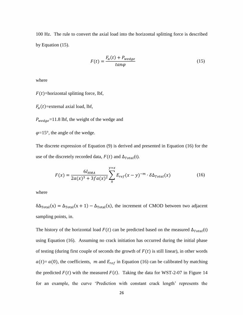
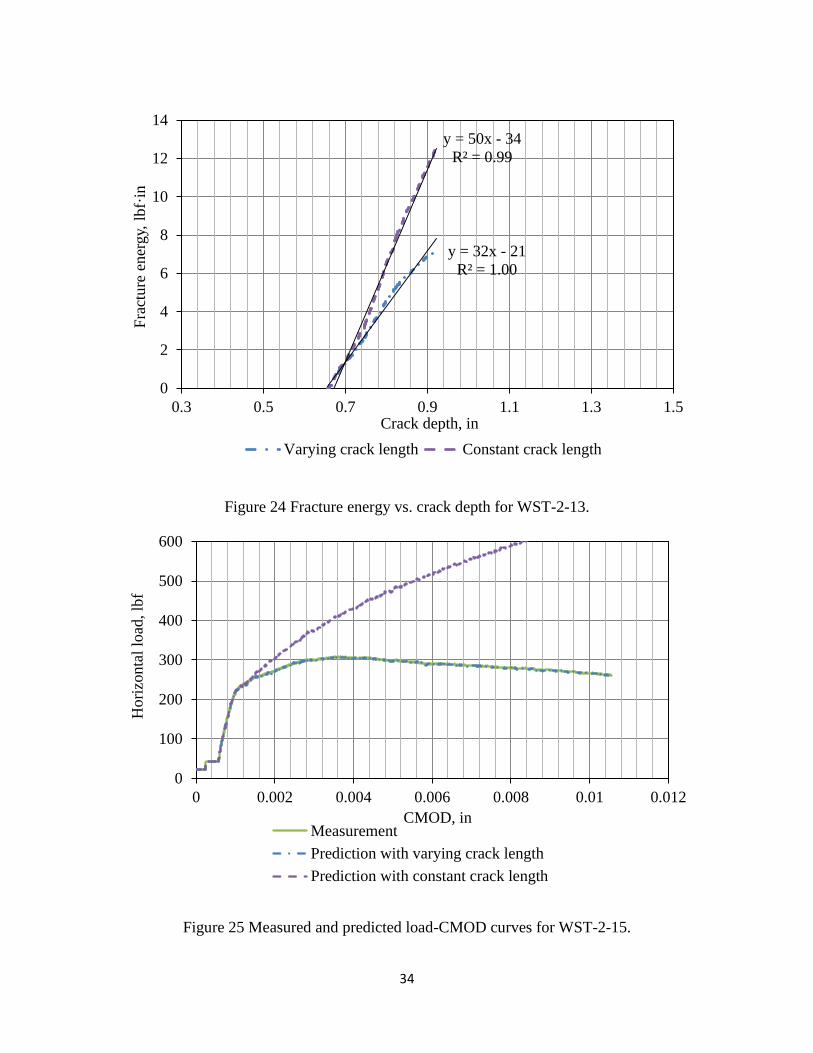
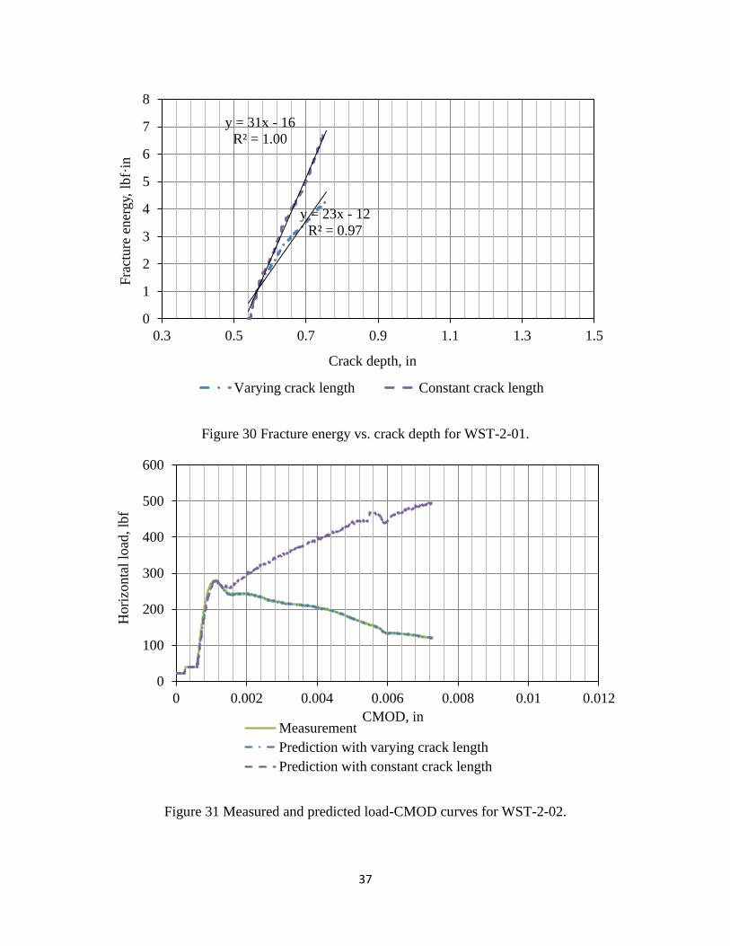
One of the byproducts of this simulation is the knowledge on the history of crack

propagation for WST-2-07. The fracture energy at any time point can also be determined

based on the integral of Equation (13). Plotting the fracture energy against the crack

depth, as shown in Figure 16, it is obvious that the slope represents the product of the

energy release rate and the width of the specimen, i.e. G×B.

The data for the other specimens that were tested under dry and room-temperature

condition was also processed using the same model, as shown in Figure 17 to Figure 42.

It is noticeable that a quick peak of the load right after the beginning of the loading is

always the result of an unstable CMOD rate, and not failure of the interface. For most of

the specimens that processed a stable constant CMOD rate, the initiation of the crack

usually occurred at 60% -90% of the peak load.

28

The accuracy of the model in predicting the crack propagation was validated by

comparing the predicted crack length with the measured crack length at the end of the test.

The comparison is presented in Table 6. Measurements of the crack length were made on

both sides of three of the specimens that did not fail abruptly. It is noteworthy that the

average of the two measurements does not necessarily represent the real crack length for

two reasons. First, the measurement only accounts for a macro crack that is visible.

Second, the profile of the crack front across the specimen is most likely nonlinear.

Nevertheless, it can still be concluded from Table 6 that the model is able to reflect

different severities of the crack propagation.

Table 6.Comparision between measured and predicted crack lengths.

Specimen Measured crack length, in

Predicted crack length, in Front Back Average

WST-2-07 0.00 0.43 0.22 0.10

WST-S-12 0.30 0.64 0.47 0.30

WST-S-14 0.00 1.18 0.59 0.77

29

Figure 14 Measured and predicted load-CMOD curves for WST-2-07.

Figure 15 Initial development of CMOD for WST-2-07.

0

100

200

300

400

500

600

0 0.002 0.004 0.006 0.008 0.01 0.012

Hori

zonta

l lo

ad, lb

f

CMOD, in

MeasurementPrediction with varying crack lengthPrediction with constant crack length

0

0.2

0.4

0.6

0.8

1

1.2

1.4

1.6

1.8

0 1 2 3 4 5

CM

OD

, m

il

Time,s

30

Figure 16 Fracture energy vs. crack depth for WST-2-07.


y = 90x - 34

R² = 0.98

y = 135x - 51

R² = 0.97

0

2

4

6

8

10

12

14

0.3 0.5 0.7 0.9 1.1 1.3 1.5

Fra

cture

ener

gy,

lbf·

in

Crack depth, in

Varying crack length Constant crack length

0

100

200

300

400

500

600

0 0.002 0.004 0.006 0.008 0.01 0.012

Hori

zonta

l lo

ad, lb

f

CMOD, in MeasurementPrediction with varying crack lengthPrediction with constant crack length

31



y = 170x - 66

R² = 1.00

y = 294x - 116

R² = 0.99

0

5

10

15

20

25

30

35

40

45

0.3 0.5 0.7 0.9 1.1 1.3 1.5

Fra

cture

ener

gy,

lbf·

in

Crack depth, in


0

100

200

300

400

500

600

0 0.002 0.004 0.006 0.008 0.01 0.012

Hori

zonta

l lo

ad, lb

f


32



y = 160x - 63

R² = 0.98

y = 199x - 79

R² = 0.99

0

5

10

15

20

25

30

0.3 0.5 0.7 0.9 1.1 1.3 1.5

Fra

cture

ener

gy,

lbf·

in

Crack depth, in


0

100

200

300

400

500

600

0 0.002 0.004 0.006 0.008 0.01 0.012

Hori

zonta

l lo

ad, lb

f

CMOD, in Measurement

Prediction with varying crack length

Prediction with constant crack length

33



y = 23x - 15

R² = 1.00

y = 64x - 45

R² = 0.98

0

5

10

15

20

25

30

35

0.3 0.5 0.7 0.9 1.1 1.3 1.5

Fra

cture

ener

gy,

lbf·

in

Crack depth, in


0

100

200

300

400

500

600

0 0.002 0.004 0.006 0.008 0.01 0.012

Hori

zonta

l lo

ad, lb

f




34



y = 32x - 21

R² = 1.00

y = 50x - 34

R² = 0.99

0

2

4

6

8

10

12

14

0.3 0.5 0.7 0.9 1.1 1.3 1.5

Fra

cture

ener

gy,

lbf·

in

Crack depth, in


0

100

200

300

400

500

600

0 0.002 0.004 0.006 0.008 0.01 0.012

Hori

zonta

l lo

ad, lb

f




35


Figure 27 Measured and predicted load-CMOD curves for WST-S-01.

y = 82x - 36

R² = 1.00

y = 173x - 81

R² = 0.97

0

5

10

15

20

25

30

35

40

45

50

0.3 0.5 0.7 0.9 1.1 1.3 1.5

Fra

cture

ener

gy,

lbf·

in

Crack depth, in


0

100

200

300

400

500

600

700

800

900

1000

0 0.002 0.004 0.006 0.008 0.01 0.012

Hori

zonta

l lo

ad, lb

f




36

Figure 28 Fracture energy vs. crack depth for WST-S-01.


y = 21x - 15

R² = 1.00

y = 68x - 56

R² = 0.97

0

5

10

15

20

25

30

35

40

45

0.3 0.5 0.7 0.9 1.1 1.3 1.5

Fra

cture

ener

gy,

lbf·

in

Crack depth, in


0

100

200

300

400

500

600

0 0.002 0.004 0.006 0.008 0.01 0.012

Hori

zonta

l lo

ad, lb

f




37



y = 23x - 12

R² = 0.97

y = 31x - 16

R² = 1.00

0

1

2

3

4

5

6

7

8

0.3 0.5 0.7 0.9 1.1 1.3 1.5

Fra

cture

ener

gy,

lbf·

in

Crack depth, in


0

100

200

300

400

500

600

0 0.002 0.004 0.006 0.008 0.01 0.012

Hori

zonta

l lo

ad, lb

f




38



y = 44x - 17

R² = 1.00

y = 77x - 30

R² = 1.00

0

2

4

6

8

10

12

0.3 0.5 0.7 0.9 1.1 1.3 1.5

Fra

cture

ener

gy,

lbf·

in

Crack depth, in


0

100

200

300

400

500

600

0 0.002 0.004 0.006 0.008 0.01 0.012

Hori

zonta

l lo

ad, lb

f




39



y = 30x - 11

R² = 1.00

y = 67x - 27

R² = 1.00

0

2

4

6

8

10

12

14

0.3 0.5 0.7 0.9 1.1 1.3 1.5

Fra

cture

ener

gy,

lbf·

in

Crack depth, in


0

100

200

300

400

500

600

0 0.002 0.004 0.006 0.008 0.01 0.012

Hori

zonta

l lo

ad, lb

f




40



y = 22x - 15

R² = 0.95

y = 39x - 27

R² = 1.00

0

2

4

6

8

10

12

14

16

0.3 0.5 0.7 0.9 1.1 1.3 1.5

Fra

cture

ener

gy,

lbf·

in

Crack depth, in


0

200

400

600

800

1000

1200

0 0.002 0.004 0.006 0.008 0.01 0.012

Hori

zonta

l lo

ad, lb

f

CMOD, in

Measurement



41



y = 29x - 13

R² = 1.00

y = 77x - 39

R² = 0.98

0

10

20

30

40

50

60

0.3 0.5 0.7 0.9 1.1 1.3 1.5

Fra

cture

ener

gy,

lbf·

in

Crack depth, in


0

100

200

300

400

500

600

0 0.002 0.004 0.006 0.008 0.01 0.012

Hori

zonta

l lo

ad, lb

f




42



y = 13x - 14

R² = 0.99

y = 20x - 23

R² = 1.00

0

1

2

3

4

5

6

7

8

9

0.3 0.5 0.7 0.9 1.1 1.3 1.5

Fra

cture

ener

gy,

lbf·

in

Crack depth, in


0

100

200

300

400

500

600

0 0.002 0.004 0.006 0.008 0.01 0.012

Hori

zonta

l lo

ad, lb

f




43


2.3.4 Analysis of WST under wet and room temperature conditions

One milled (WST-S-04) and two unmilled (WST-S-12 and WST-S-14) specimens were

saturated before the testing in order to study the effect of moisture on the energy release

rate. The weight of these specimens had been monitored, as shown in Table 7, since they

were sent back to the moisture room. The specimens were saturated after 27 days as

indicated by the negligible rate of weight change at 27 days, as presented in Figure 43.

Table 7 Weight change of specimens

Date Time Days in

moisture room

Weight of specimen, lbs

WST-S-04 WST-S-12 WST-S-14

5/22/2012 19:00 0 13.000 17.419 14.919

5/24/2012 11:30 2 13.055 17.486 14.974

5/25/2012 13:40 3 13.061 17.493 14.982

5/27/2012 14:20 5 13.066 17.504 14.992

5/28/2012 12:00 6 13.067 17.505 14.994

y = 13x - 14

R² = 0.99

y = 20x - 23

R² = 1.00

0

0.2

0.4

0.6

0.8

1

1.2

1.4

1.6

1.8

0 0.5 1 1.5 2 2.5

Fra

cture

ener

gy,

lbf·

in

Crack depth, in


44

6/8/2012 21:00 17 13.079 17.533 15.015

6/14/2012 13:00 23 13.084 17.539 15.020

6/18/2012 13:00 27 13.085 17.542 15.022

Figure 43Weight chart for specimens stored in moisture room.

The data for the all three specimens that were tested under wet and room-temperature

condition were processed using the model presented previously and the resulting energy

release rates were calculated. The results are presented in Figure 44 to Figure 49.

0

0.1

0.2

0.3

0.4

0.5

0.6

0.7

0.8

0 5 10 15 20 25 30

Chan

ge

in w

eight,

%

Days

WST-S-4 WST-S-12 WST-S-14

45



0

100

200

300

400

500

600

0 0.002 0.004 0.006 0.008 0.01 0.012

Hori

zonta

l lo

ad, lb

f


y = 17x - 12

R² = 1.00

y = 46x - 35

R² = 0.98

0

5

10

15

20

25

0.3 0.5 0.7 0.9 1.1 1.3 1.5

Fra

cture

ener

gy,

lbf·

in

Crack depth, in


46



0

100

200

300

400

500

600

0 0.002 0.004 0.006 0.008 0.01 0.012

Hori

zonta

l lo

ad, lb

f




y = 23x - 12

R² =1.00

y = 47x - 26

R² = 0.99

0

2

4

6

8

10

12

14

0.3 0.5 0.7 0.9 1.1 1.3 1.5

Fra

cture

ener

gy,

lbf·

in

Crack depth, in


47



2.3.5 Analysis of WST under dry and freezing conditions

0

100

200

300

400

500

600

0 0.002 0.004 0.006 0.008 0.01 0.012

Hori

zonta

l lo

ad, lb

f




y = 19x - 10

R² =1.00

y = 56x - 34

R² = 0.97

0

5

10

15

20

25

30

0.3 0.5 0.7 0.9 1.1 1.3 1.5

Fra

cture

ener

gy,

lbf·

in

Crack depth, in


48

Three milled (WST-2-10, WST-2-11 and WST-2-14) and three unmilled (WST-2-04 to

WST-2-06) specimens were stored in a freezer before testing, along with a dummy WST

specimen that is of the same geometry but instrumented with three thermocouples. The

three thermocouples denoted by ‘edge’, ‘half way’ and ‘middle’ in Figure 50 were

embedded at the interface, 0.5 in, 1.5 in and 3 in away from the side of dummy specimen,

respectively. It is obvious that 40 hours of storage in the freezer is enough to cool the

specimen to as low as 6 °F. Since there is no environmental chamber for the actuator, the

loading was carried out under room temperature. During the testing that is approximately

10 minutes long, the temperature of specimens increased by about 2 to 4 °F as shown in

Figure 51, depending on where the temperature was measured. The temperature at the

edge rose quicker than the temperature deep inside. Nevertheless, it is fair to assume the

test was carried out at a relatively constant low temperature, at least for the comparison

between the room-temperature and frozen WST specimens.

Figure 50 Change of temperature for the frozen specimens in the freezer.

0

10

20

30

40

50

60

70

80

0 500 1000 1500 2000 2500

Tem

per

ature

, °F

Time, minute

Thermocouple at edge Thermocouple at halfway Thermocouple at middle

Testing

Refrigiator resting

49

Figure 51 Change of temperature for the frozen specimens during the test.

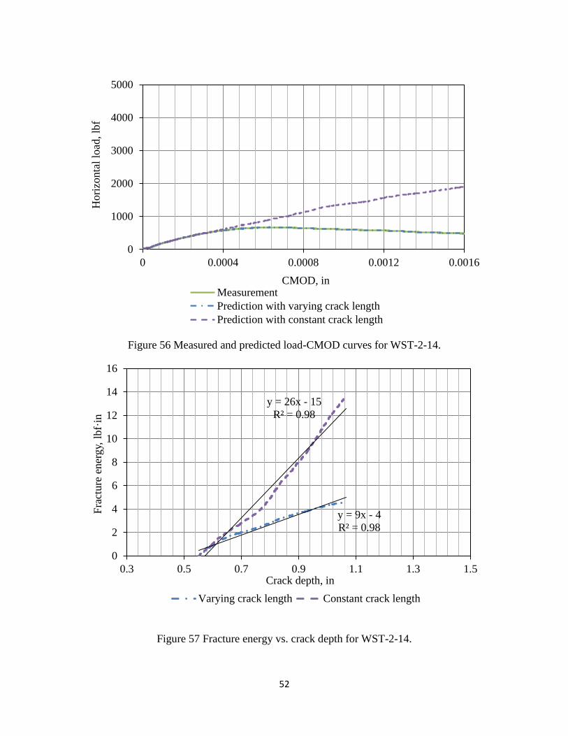
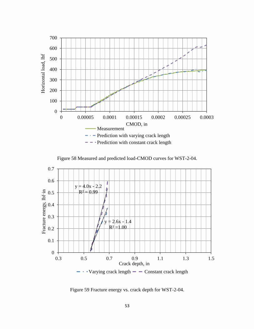
The data for the all dry- and frozen specimens were processed using the model presented

previously and the resulting energy release rates were calculated. The results are

presented in Figure 52 to Figure 63.

0

5

10

15

20

25

30

2340 2345 2350 2355 2360 2365 2370 2375 2380

Tem

per

atu

re, °F

Time, minute

Thermocouple at edge Thermocouple at halfway Thermocouple at middle

Beginning of test Ending

50



0

1000

2000

3000

4000

5000

0 0.0004 0.0008 0.0012 0.0016

Hori

zonta

l lo

ad, lb

f




y = 17x - 6

R² = 0.98

y = 84x - 36

R² = 0.96

0

5

10

15

20

25

30

35

40

45

50

0.3 0.5 0.7 0.9 1.1 1.3 1.5

Fra

cture

ener

gy,

lbf·

in

Crack depth, in


51



0

1000

2000

3000

4000

5000

0 0.0004 0.0008 0.0012 0.0016

Hori

zonta

l lo

ad, lb

f




y = 33x - 13

R² = 0.98

y = 79x - 32

R² = 0.98

0

2

4

6

8

10

12

14

16

18

0.3 0.5 0.7 0.9 1.1 1.3 1.5

Fra

cture

ener

gy,

lbf·

in

Crack depth, in


52



0

1000

2000

3000

4000

5000

0 0.0004 0.0008 0.0012 0.0016

Hori

zonta

l lo

ad, lb

f




y = 9x - 4

R² = 0.98

y = 26x - 15

R² = 0.98

0

2

4

6

8

10

12

14

16

0.3 0.5 0.7 0.9 1.1 1.3 1.5

Fra

cture

ener

gy,

lbf·

in

Crack depth, in


53



0

100

200

300

400

500

600

700

0 0.00005 0.0001 0.00015 0.0002 0.00025 0.0003

Hori

zonta

l lo

ad, lb

f




y = 2.6x - 1.4

R² =1.00

y = 4.0x - 2.2

R² = 0.99

0

0.1

0.2

0.3

0.4

0.5

0.6

0.7

0.3 0.5 0.7 0.9 1.1 1.3 1.5

Fra

cture

ener

gy,

lbf·

in

Crack depth, in


54



0

100

200

300

400

500

600

0 0.0001 0.0002 0.0003 0.0004

Hori

zonta

l lo

ad, lb

f




y = 2.7x - 1.6

R² =0.98

y = 3.6x - 2.1

R² = 0.99

0

0.1

0.2

0.3

0.4

0.5

0.6

0.3 0.5 0.7 0.9 1.1 1.3 1.5

Fra

cture

ener

gy,

lbf·

in

Crack depth, in


55



0

200

400

600

800

1000

1200

1400

1600

0 0.0001 0.0002 0.0003 0.0004 0.0005

Hori

zonta

l lo

ad, lb

f




y = 2.7x - 1.6

R² =0.98

y = 3.4x - 2.1

R² = 0.99

0

0.05

0.1

0.15

0.2

0.25

0.3

0.3 0.5 0.7 0.9 1.1 1.3 1.5

Fra

cture

ener

gy,

lbf·

in

Crack depth, in


56

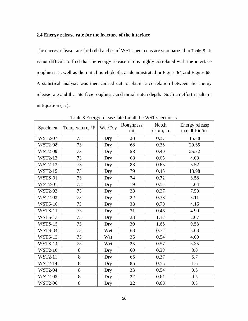
2.4 Energy release rate for the fracture of the interface

The energy release rate for both batches of WST specimens are summarized in Table 8. It

is not difficult to find that the energy release rate is highly correlated with the interface

roughness as well as the initial notch depth, as demonstrated in Figure 64 and Figure 65.

A statistical analysis was then carried out to obtain a correlation between the energy

release rate and the interface roughness and initial notch depth. Such an effort results in

in Equation (17).

Table 8 Energy release rate for all the WST specimens.

Specimen Temperature, °F Wet/Dry Roughness,

mil

Notch

depth, in

Energy release

rate, lbf·in/in2

WST2-07 73 Dry 38 0.37 15.48

WST2-08 73 Dry 68 0.38 29.65

WST2-09 73 Dry 58 0.40 25.52

WST2-12 73 Dry 68 0.65 4.03

WST2-13 73 Dry 83 0.65 5.52

WST2-15 73 Dry 79 0.45 13.98

WSTS-01 73 Dry 74 0.72 3.58

WST2-01 73 Dry 19 0.54 4.04

WST2-02 73 Dry 23 0.37 7.53

WST2-03 73 Dry 22 0.38 5.11

WSTS-10 73 Dry 33 0.70 4.16

WSTS-11 73 Dry 31 0.46 4.99

WSTS-13 73 Dry 33 1.12 2.67

WSTS-15 73 Dry 30 1.68 0.53

WSTS-04 73 Wet 68 0.72 3.03

WSTS-12 73 Wet 35 0.54 4.00

WSTS-14 73 Wet 25 0.57 3.35

WST2-10 8 Dry 60 0.38 3.0

WST2-11 8 Dry 65 0.37 5.7

WST2-14 8 Dry 85 0.55 1.6

WST2-04 8 Dry 33 0.54 0.5

WST2-05 8 Dry 22 0.61 0.5

WST2-06 8 Dry 22 0.60 0.5

57

Figure 64 Energy release rate vs. roughness.

Figure 65 Energy release rate vs. initial notch depth.

(17)

0

5

10

15

20

25

30

0 10 20 30 40 50 60 70 80 90

Ener

gy r

elea

se r

ate,

lbf·

in/i

n2

Roughness, mil

Milled-Dry Milled-Wet Unmilled-Dry Unmilled-Wet

0

5

10

15

20

25

30

0.0 0.5 1.0 1.5 2.0

Ener

gy r

elea

se r

ate,

lbf·

in/i

n2

Notch depth, in

Milled-Dry Milled-Wet Unmilled-Dry Unmilled-Wet

58

The values for the coefficients in Equation (17) are presented in Table 9 and are

dependent on the calibration database.

Table 9. Coefficients in Equation (17).

Set Database

1 Milled-dry specimens -1.89 1.03 -3.42 0.95

2 Unmilled-dry specimens -1.089 0.914 -1.594 0.80

3 All dry specimens -0.8544 0.711 -1.916 0.83

4 All frozen specimens -2.058 0.736 -3.10 0.87

In Figure 66, it compares the measured and predicted energy release rates.

Figure 66 Comparison between measured and predicted energy release rate, based on

Equation (17) and coefficient Sets 1 and 2 from Table 9.

The energy release rate for all the milled specimens is predicted using Equation (17)

along with the coefficients from Set 1 in Table 9 and the energy releaser rate for all the

unmilled specimens is calculated with coefficients from Set 2. It is interesting to observe

0

5

10

15

20

25

30

0 5 10 15 20 25 30

Pre

dic

ted e

ner

gy r

elea

se r

ate,

lbf·

in/i

n2

Measured energy release rate, lbf·in/in2

Milled-Dry Milled-Wet Unmilled-DryUnmilled-Wet Milled-Dry-Frozen Unmilled-Dry-Frozen

59

that no distinct difference is found between the dry and wet specimens. On the other

hand, the frozen specimens present much smaller energy release rate than the room-

temperature specimens. Therefore, new coefficients were determined for the frozen

specimens, i.e. Set 4 in Table 9. Based on coefficient Sets 1, 2 and 4, the predicted

energy release rate for all the specimens is compared with the measurements again as

shown in Figure 67, where a good agreement is observed.

Figure 67 Comparison between measured and predicted energy release rate, based on

Equation (17) and coefficient Sets 1, 2 and 4 from Table 9.

The parameters in Equation (16), i.e. m and Eref, obtained during the modeling are

presented in Table 10. For the milled and room-temperature specimens, m varies

between 0.4 and 0.8 and Eref varies between 1400 and 16000. For the unmilled and

room-temperature specimens, m varies between 0.5 and 0.7 and Eref varies between 800

and 7700. For the milled and frozen specimens, m varies between 0.16 and 0.25 and Eref

0

5

10

15

20

25

30

0 5 10 15 20 25 30

Pre

dic

ted s

pec

ific

ener

gy,

lbf·

in/i

n2

Measured specific energy, lbf·in/in2

Milled-Dry Milled-Wet Unmilled-Dry

Unmilled-Wet Milled-Dry-Frozen Unmilled-Dry-Frozen

60

varies between 28000 and 84500. For the unmilled and frozen specimens, m varies

between 0.2 and 0.3 and Eref varies between 20000 and 42000.

Four conclusions can be made based on the comparison among above mentioned ranges.

First, the model developed in this study considers the interface as a viscoelastic medium.

The backcalculated m and Eref should reflect the characteristic of the interface while not

only limited to the characteristic of the HMA. Second, Eref is generally greater for milled

specimens than unmilled specimens, indicating that the interface made of milled asphalt

is stiffer. Third, m depends on temperature and frequency, while not milling condition.

This is supported by the fact that milled and unmilled specimens present similar m-value

at the same temperature. The deviation of the m at the same temperature is believed due

to the different initial loading rates among the specimens as well as the deviation of the

HMA and PCC properties from specimen to specimen. Fourth, the deviation of m and

Eref for the milled specimens is much larger than that for the unmilled specimens,

indicating the possibility of multiple failure paths for the milled specimens.

Table 10. m and Eref for all the WST specimens.

Specimen Temperature, °F Wet/Dry Milling m Eref

WST2-07 73 Dry Milled 0.8 1410

WST2-08 73 Dry Milled 0.67 1750



WST2-13 73 Dry Milled 0.57 7500

WST2-15 73 Dry Milled 0.58 5200

WSTS-01 73 Dry Milled 0.4 16000

WST2-01 73 Dry Unmilled 0.69 1600



WSTS-10 73 Dry Unmilled 0.55 5400



61


WSTS-04 73 Wet Milled 0.5 10000

WSTS-12 73 Wet Unmilled 0.7 1550

WSTS-14 73 Wet Unmilled 0.6 3750

WST2-10 8 Dry Milled 0.16 47000

WST2-11 8 Dry Milled 0.16 28000

WST2-14 8 Dry Milled 0.25 84500




The failure surfaces for some of the WST specimens are presented in Figure 68 to Figure

73. For the milled and room-temperature specimens, the failure might be either along the

interface (WST-2-09) or in the asphalt (WST-S-01). Furthermore, the existence of an

angle between the milling and the loading direction does not guarantee a rougher failure,

as can be seen by comparing WST-2-09 (0° milling angle) with WST-2-15 (45° milling

angle).

A much cleaner failure surface can be found for the unmilled and room-temperature

specimens (WST-2-01) than the milled and room-temperature specimens, although the

black spots on the failure surface indicate that the tensile failure of asphalt is also

involved in the fracture failure of this specimen. This comparison implies that the

interface made from milled HMA is much tougher.

There is less HMA stuck on the concrete half for the frozen specimens than for the room-

temperature specimens, which is true for both milled (WST-2-09 vs. WST-2-11) and

unmilled WST specimens (WST-2-01 vs. WST-2-05). This implies that the interface is

stiffer at a lower temperature.

62

Figure 68 Failure surfaces of milled, dry and room-temperature specimen, WST-2-09.

Figure 69 Failure surfaces of milled, dry and room-temperature specimen, WST-S-01.

63

Figure 70 Failure surfaces of 45° milled, dry and room-temperature specimen, WST-2-15.

Figure 71 Failure surfaces of unmilled, dry and room-temperature specimen, WST-2-01.

64

Figure 72 Failure surfaces of milled, dry and frozen specimen, WST-2-11.

Figure 73 Failure surfaces of unmilled, dry and frozen specimen, WST-2-05.

2.5 Summary

A wedge splitting test setup is developed to fracture the PCC-HMA composite specimens

along the interface in Mode I. The tests were carried out with CMOD control and the

load-CMOD data was recorded both pre- and post- peak load. A model was then

established based on beam theory and viscoelasticity to analyze the data. As a result of

the modeling, the progress of the crack as well as the energy release rate was determined

65

for every specimen. An equation is then proposed to relate the energy release rate with

the interface roughness, initial notch depth and temperature. Furthermore, it is found that

the m-value used in the model is a function of the temperature and loading frequency,

while not depending on the milling condition. It is also found that the parameter Eref

indicates the stiffness of the interface. The interface with milled HMA is much stiffer

than the one with unmilled HMA.

66

3. COHESIVE ELEMENT MODELING OF THE INTERFACE

Springs have been traditionally used in finite element models to simulate the bond

between overlay and the underlying layer. Uniform spring stiffness is usually assigned.

The development of interface debonding is usually reflected by reducing the spring

stiffness. There are two apparent shortcomings with using springs with uniform elastic

modulus to model the interface. First, the damage to the interface consisted of both

recoverable and irrecoverable (damage) deformations. Elastic springs are not capable of

capturing the damage. Second, the deformation of the interface under wheel loads is not

uniform and thus the interface elements are damaged differently. The initial condition of

all the interface elements might be identical, but they will deviate as the fatigue loading is

applied.

In this chapter, it was proposed that the interface fracture of UTW could be modeled

using superimposed cohesive zone models (CZMs). The interface cracking was first

broken down into several types of constitutive failure. Root CZMs were proposed to

represent the constitutive failure types. It is important to note that the model inputs for

each root CZM are material dependent. In such a way the inputs for the root models can

be established based on small-scale laboratory tests, such as wedge splitting test, and then

be applied to the analysis of fracture at larger scales, for example the calculation of

energy release rate in finite element modeling of UTW slabs. The WST results from the

last chapter were used to determine the fracture properties for the UTW interface based

on inverse analysis. Furthermore, the effect of milling and specimen size on the fracture

properties was also investigated.

67

3.1 Cohesive Zone Model

Cohesive zone models (CZM) are widely used to simulate the progression of nonlinear

cracking. In a CZM, the crack path is represented by two adjacent but separated surfaces

whose separation indicates the opening of the crack. Tractions are assumed to exist

between the two separating surfaces in order to avoid the stress singularity at the crack tip

in linear elastic fracture mechanics. The constitutive relationship for CZM is a traction-

separation law (TSL). A basic TSL includes three phases. In the first (no-damage

opening) phase, traction increases with the separation without any damage caused until

the peak traction is reached. The second phase is the softening phase, where the traction

decreases with further separation due to the occurrence and accumulation of damage.

The last phase is characterized by the cohesive separation exceeding a critical value

resulting in zero traction and proceeding cracks. So far, the basic TSL has mutated to

various shapes in order to reflect different cracking mechanisms in different materials.

The typical TSLs that have been used to model concrete, asphalt, or the interface of

composites are summarized in Figure 74.

Figure 74 Traction-separation laws (a) for concrete (b) for asphalt and interfaces

68

3.1.1 CZM for concrete

A CZM with linear softening phase (i.e. bilinear TSL) was first proposed by Hillerborg et

al. (1979) to model the quasi-brittle fracturing of plain concrete. In Figure 74 (a), this

CZM presents a softening phase, where the traction linearly decreases with increased

separation, which reflects the damage accumulation due to plasticity in quasi-brittle

materials (Ural et al., 2009). CZMs with bilinear softening phase are more often used for

the modeling of plain concrete fracture (Guinea et al., 1994 and Bazant and Becq-

Giraudon 2002). The bilinear softening reflects the aggregate bridging across the crack

in addition to the plastic damage accumulation. For the fracture of fiber reinforced

concrete, Park et al.(2010) introduced multi-linear softening that presents an additional

requirement of fracture energy relative to the bilinear softening to take into account the

fiber bridging during fracture.

3.1.2 CZM for asphalt

Kim et al. (2008) employed a CZM with bilinear TSL to simulate the fracture of asphalt

at low temperature (-10 °C). The linear softening was believed to reflect the damage

mechanism due to plastic deformation. Power-law softening was compared with linear

softening by Song et al. (2008) and it was concluded that the power law was better in

analyzing the fracture of asphalt at low temperatures (-10 °C to -30 °C).

3.1.3 CZM for interface

http://www.sciencedirect.com/science/article/pii/S0008884601007232


69

Mohammed and Liechti (2000) used a bilinear TSL to study the fracture between

aluminum and epoxy. The properties of TSL were inversely determined from third point

bending measurements. The model showed good predictability for failures with various

initial flaw sizes. Another TSL with bilinear softening law was adopted by Li et al. (2005)

to study the fracture of adhesively bonded fiber reinforced composites. It is more popular

to model the facture of adhesively bonded joints using a trapezoidal TSL, as shown in

Figure 74 (b) (Tvergaard and Hutchinson, 1992; Feraren and Jensen, 2004 and Alfano et

al., 2007). The shape of a TSL affects its performance in modeling the interfacial

fracture. Alfano et al. (2009) conducted a comparison between the bilinear, linear-

exponential, and trapezoidal TSLs in modeling the aluminum-epoxy joint fracture. The

three TSLs yield different predictions despite the fact that the cohesive strength as well as

the fracture energy is the same among models.

3.2 CZM for Interface of UTW

An examination of the UTW specimen after failure revealed that the failure is composed

of many subcritical failures such as: the cement/asphalt matrix debonding,

cement/exposed aggregate debonding, aggregate pull-out, aggregate cracking, and asphalt

cracking; instead of one critical failure. Figure 75 shows a picture of the interface after

fracture for both milled and unmilled specimens. Since the fracture of unmilled

specimens is cleaner, Figure 75 (a) was first examined. Six failure types could be

identified, for which the location and mechanisms are summarized in Table 11.

Table 11 Location and mechanism for subcritical failures.

Failure Type Location Mechanism

70

(I) Interface between concrete and exposed asphalt aggregates Adhesion*

(II) Interface between concrete and asphalt matrix Adhesion

(III) Asphalt matrix Cohesion**

(IV) Aggregate fracture Cohesion

(V) Pullout of aggregates from asphalt matrix Adhesion

(VI) Voids at the concrete/asphalt interface N/A

*Adhesion is the bonding force between two different materials

**Cohesion is the bonding force within the same material

Type (I) failure is obvious since the shape of the failures agrees with the shape of the

exposed aggregates before concrete casting. Type (II) failure is the adhesion failure

between the concrete and asphalt matrix, which consists of two mechanisms. After

magnification, it is apparent that the failure is actually a mix between the cement

adhesion failure (grey dots within the area) and the asphalt adhesion failure (darker dots

within the area) but the cement adhesion failure is predominant. Type (III) failure is

easily detected when the asphalt matrix cracks leaving chunks of asphalt adhered to the

concrete side of the failure plane. Type (IV) failure is mostly found when there are

aggregates of poor quality, such as sandstone. Type (V) failure occurs when the cement

adhesion on the exposed aggregates is greater than the asphalt adhesion. Type (VI) is a

void at the interface, where no hardened cement is present and thus the interface strength

is zero.

71

Figure 75 Fractured UTW interface on the concrete side (a) a unmilled specimen and (b)

a milled specimen: (I) adhesion failure between concrete and aggregate (II) adhesion

failure between concrete and asphalt matrix (III) asphalt failure (IV) aggregate facture (V)

aggregate pullout and (VI) voids.

Although the fracture of the milled specimen, Figure 75 (b), is more difficult to interpret,

the same failure types can still be concluded after carefully comparing Figure 75 (b) with

the asphalt surface before concrete casting. There are some differences in the fracture

between the milled and unmilled specimens. First, the amount of Type (I) and Type (II)

failures is significantly lower in the milled specimen. This is because the texture of the

exposed aggregates and asphalt matrix is roughened by the milling operation resulting in

a stronger bond between them and the fresh concrete. As a result, the cracking path tends

to go through the asphalt. More interestingly, a closer examination of the Type (II)

failure reveals that there is nearly no bond at locations where the milling operation

created grooves. These grooves are approximately 0.25-1 inches deep, relative to the

other post-milling area where there is evenly distributed crushed aggregates/roughened

asphalt matrix. Aggregates from the fresh concrete could bridge and shield the grooves

preventing cement from bonding to the milled asphalt at the bottom of the grooves.

Moreover, dust and debris may be deposited there before concrete placement and behave

72

as a bond breaker, preventing bonding even if fresh cement paste is able to enter the

grooves. The second difference is that Type (III), (IV) and (V) failures become

predominant, which is also a product of the milling and compliments the decrease of

Type (I) and (II) failures.

It can be concluded from the above examination that an effective CZM for the interfacial

fracture of UTW should be based on the superimposition of certain root CZMs. Each of

the root CZMs should reflect one of the subcritical types of failure. The advantage of

using such a superimposition approach is as follows. First, the root CZMs are only

dependent on material properties. Therefore, they can be used for modeling at multiple

scales. Second, the shape of the overall CZM after superimposition is a function of the

interfacial composition. Theoretically, it can be any shape. Such flexibility is desirable

when the overall CZM is determined based on inverse analysis, since it is capable of

capturing all the possible subcritical failure mechanisms. If a fixed shape is pre-selected

for the overall TSL, the numbers of failure mechanisms it can represent is fixed

beforehand too.

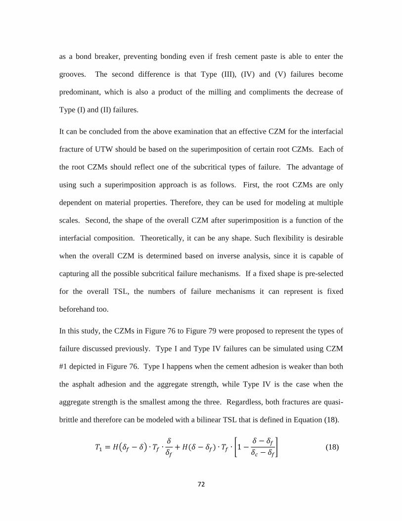
In this study, the CZMs in Figure 76 to Figure 79 were proposed to represent the types of

failure discussed previously. Type I and Type IV failures can be simulated using CZM

#1 depicted in Figure 76. Type I happens when the cement adhesion is weaker than both

the asphalt adhesion and the aggregate strength, while Type IV is the case when the

aggregate strength is the smallest among the three. Regardless, both fractures are quasi-

brittle and therefore can be modeled with a bilinear TSL that is defined in Equation (18).

( )

[

] (18)

73

where is the heaveside step function; is the peak traction, psi; is the separation at

the maximum traction and is the critical separation beyond which the traction is zero.

The ITZ also includes an asphalt component, whose deformation is significant.

Therefore the fracture behavior of asphalt should be considered when establishing the

CZM. The fracture of the asphalt during monotonic opening is represented by an

exponential TSL in Equation (19).

( ) (

)

[

]

(19)

where and are the shape factors of the TSL.

Since the asphalt is not fractured in Type I and Type IV failures, it should unload after

either the cement/aggregate interface or the aggregate starts to damage. The loading and

unloading paths for the asphalt will not coincide. There should be a difference between

the loading and unloading curves that is induced by the dissipation of energy due to

viscous deformation. Therefore, the traction-separation relationship for unloading should

not be described by Equation (19). Assuming the initial slope of the unloading curve is

the same as the initial slope of the loading curve, i.e. Equation (20), the TSL for asphalt

in a loading-unloading scenario before the peak traction can be derived as in Equation

(21).

(20)

(

)

[

] (21)

74

where is the separation when the unloading starts and .

Hence, the overall TSL for CZM #1 can be obtained by assembling two root models,

namely the bilinear TSL in Equation (18) and the loading-unloading curve of asphalt in

Equation (21) in series, resulting in Equation (22).

( ) ( ( ) ) (22)

where is the inverse function of , i.e.

and .is in Equation (21)

Figure 76 Cohesive zone model #1

Type II failure occurs when the cement/asphalt matrix adhesion is weaker than the

asphalt cohesion. This type of failure is modeled by CZM # 2 presented in Figure 77. It

is assumed that the TSL in Equation (19), but with different parameters, is also suitable

for defining the cement/asphalt matrix adhesion, considering that the adhesion is

primarily cementitous in nature. Similar to CZM #1, the overall TSL for CZM #2 is a

combination of the cement/asphalt matrix TSL and the loading-unloading curve of

asphalt in series, as defined in Equation (23).

75

( ) ( ( ) ) (23)


CZM #3 in Figure 78 is used to model Type III and Type V failure. For the ITZ in Figure

78, cracking will happen in the asphalt when both the cement-aggregate adhesion and the

aggregate cohesion are stronger than the asphalt cohesion. The cracking of asphalt might

happen to the asphalt matrix, the aggregates in the asphalt, or along the interface between

asphalt matrix and the embedded aggregates. However, for simplicity, the same TSL is

assumed for all the possible asphalt fractures. Therefore, the overall TSL for CZM #3

can be derived as shown in Equation (24), by combining Equation (18) that describes the

pre-peak loading and unloading behavior of the bilinear TSL and Equation (19) that

defines the asphalt fracture under monotonic loading.

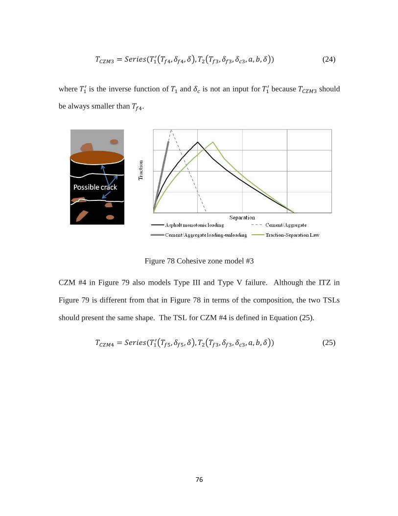
76

( ) ( ) (24)

where is the inverse function of and is not an input for

because should

be always smaller than .


CZM #4 in Figure 79 also models Type III and Type V failure. Although the ITZ in

Figure 79 is different from that in Figure 78 in terms of the composition, the two TSLs

should present the same shape. The TSL for CZM #4 is defined in Equation (25).

( ) ( ) (25)

77


The overall traction-separation law for UTW can be determined as in Equation (26) after

proportionally combining CZMs #1 to #4 (Equations (22) to (25)) in parallel.

∑

(26)

where =1 to 5, =1 to 3 and is the occupancy of the interface by each failure type, i.e.

to .

Theoretically, the fifteen fracture parameters in Equation (26) could be established based

on a couple of laboratory fracture tests that target one root CZM at a time. For example,

and could be obtained from the Mode I fracture test between aged asphalt

matrix and cement. However, it is nearly impossible to guarantee 100% failure at the

interface and furthermore it is extremely difficult to manufacture the specimens,

especially at a testable size. In this study, the results from the wedge splitting test are

78

used to determine the fracture properties of the root CZMs. An inverse analysis approach

can be employed to extract the properties from the complicated WST failure.

3.3 Wedge Splitting Test Setup and Results

The experimental setup for the WST and a UTW specimen prepared for the WST are

presented in Figure 80. A small square of material is removed from the central portion of

the specimen. The clip gage for monitoring the crack mouth opening displacement

(CMOD) is placed in this opening. A notch is cut in the central portion of this region at

the interface to establish the location of crack initiation. A guide notch of approximately

¼ in/6 mm deep is also made on both faces of the specimen to ensure the crack

propagates along the interface. Two steel caps with bearings attached are placed on the

specimen on each side of the removed region. The axial load applied to the wedge is

transformed to a pair of horizontal splitting forces and a pair of vertical forces at the steel

bearings. Since the linear supports were aligned with the steel bearings, the moment

causing cracks at the interface is mainly caused by the pair of splitting forces. The

recorded result from the WST is the axial load-CMOD curve. The splitting force is

related to the axial load as well as the angle of the wedge during quasi-static loading and

thus the splitting force-CMOD curve can be derived.

79

Figure 80 Wedge splitting test configuration.

This study uses the test results of dry UTW specimens at room temperature, i.e.

72 °F/22 °C. The fracture is induced by quasi-static loading with CMOD rate of 20

mils/min. The asphalt specimens were extracted from an in-situ asphalt pavement, a

portion of which has milled texture while the rest of the pavement was unmilled to study

the effect of HMA surface. The sand patch test (ASTM-E965-96) was conducted to

quantify the asphalt roughness in terms of a characteristic depth. A rougher surface is

indicated by a larger value of the characteristic depth. The depth (D in Figure 80) of

unmilled HMA specimens is 4-5 in, compared to 3-3.5 in for the milled specimens. The

height and width of the asphalt specimens are both 6 in. The nominal height and depth of

the cut are 2 in and 1 in, respectively. A standard depth for the initial notch is 0.5 in

except the specimens with different notch depths which were used to study the effect of

flaw size on the interfacial fracture.

Representative WST results are presented in Figure 81. Specimens 2-1, S-11 and S-15 are

unmilled. S-11 and S-15 share the same dimensions and similar asphalt roughness, as

seen in Table 12. The difference in load-CMOD behavior between them is because the

80

initial notch depth for S-15 is 44% of the nominal contact length (H-C.H) relative to 11%

for S-11. Specimen 2-1 has a surface roughness that is only 20 mils compared to 32 mils

for S-11, which might explain the difference between 2-1 and S-11. For the two milled

specimens S-1 and 2-12, S-1 exhibited a much larger proportion of Type III failure

(failure of the asphalt matrix), than 2-12. The only apparent difference between them is

that the concrete of S-1 is 25% thinner than 2-12.

Table 12 Dimensions of WST specimens shown in Figure 81.

2-1 S-11 S-15 S-1 2-12

Dimensions as

illustrated in

Figure 80, in

Asphalt

D 3.82 3.94 3.66 2.64 2.56

H 5.94 5.51 5.47 5.51 5.75

C.D 1.38 1.18 1.10 1.02 1.06

C.H 2.05 1.85 1.77 1.89 1.85

W 5.71 5.83 5.71 5.91 5.71

Concrete

D 4.33 3.35 3.43 2.28 3.15

H 6.02 5.55 5.55 5.51 5.71

C.D 1.10 0.91 1.10 1.10 1.14

C.H 2.01 1.89 1.77 1.93 1.77

W 5.71 5.83 5.71 5.91 5.71

Notch depth, in 0.55 0.47 1.69 0.71 0.67

Contact area, in2 19.4 18.5 11.8 17.2 18.6

Interface roughness based on sand patch

test, mil 20 32 32 76 68

81

Figure 81 Typical splitting force-CMOD curves from the wedge splitting test of UTW.

The dependence of the WST results on the specimen size, i.e. specimen thickness and

initial notch depth, implies that the size of the fracture process zone for the interfacial

cracks is so large that it is more or less comparable to the specimen size. Therefore, the

effect of specimen size should also be studied in addition to the asphalt roughness, when

using the WST results to determine the fracture properties of the cohesive zone models.

3.4 Finite Element Implementation of the CZM

The finite element package ABAQUS was used in the study to implement the cohesive

zone models. A UTW specimen in the WST setup is modeled and presented in Figure 82.

Concrete and asphalt were modeled as homogenous materials. Concrete was treated as

an elastic material. The elastic modulus and Poisson’s ratio for the concrete are 4 million

psi and 0.2, which were obtained from laboratory testing complying with ASTM C469.

0

50

100

150

200

250

300

0 2 4 6 8 10 12

Spli

ttin

g f

orc

e, l

bf

CMOD, mil

2-1 S-11 S-15 S-1 2-12

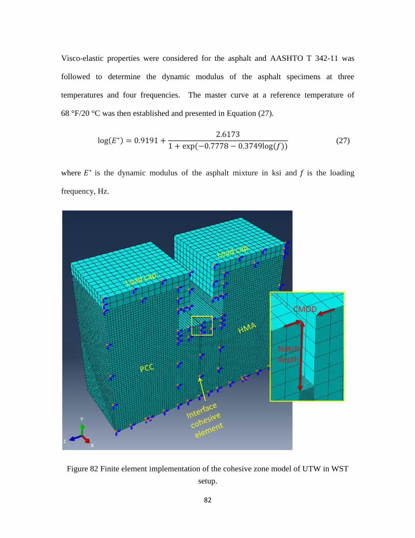
82

Visco-elastic properties were considered for the asphalt and AASHTO T 342-11 was

followed to determine the dynamic modulus of the asphalt specimens at three

temperatures and four frequencies. The master curve at a reference temperature of

68 °F/20 °C was then established and presented in Equation (27).

(27)

where is the dynamic modulus of the asphalt mixture in ksi and is the loading

frequency, Hz.

Figure 82 Finite element implementation of the cohesive zone model of UTW in WST

setup.

83

The interface was modeled with the overall cohesive zone model described by Equation

(26). In ABAQUS, strain, instead of separation, is used to define the critical

displacement of a CZM. Therefore, the thickness of the cohesive zone is set constant,

resulting in a one-one mapping between the required strain and the separation defined in

Equation (26). Multiple mechanisms are available in ABAQUS to define the strain

softening of a CZM. This study employed the damage-displacement relation that could

be converted from a TSL. The damage variable in such a relation is defined by Equation

(28), where the stiffness can be obtained by dividing the current traction with the current

strain.

(28)

where are the stiffness components at the normal and shear directions of the

interface elements, predicted by the linear traction-separation law without damage, and D

is the scalar damage variable.

Only half of the specimen was simulated due to the symmetry. The convergence of the

model in terms of both mesh size and time step was validated. Using the model, the

splitting force-CMOD curve for a specific specimen can be simulated for a specimen

with any given TSL.

3.5 Inverse Analysis for the CZM Parameters Based on WST Results

Inverse analysis was used to determine the parameters of the CZM including the TSL.

The inverse analysis can be described by the optimization problem in Equation (29). The

goal is to minimize the error between the predicted P-CMOD curve and the measured P-

84

CMOD curve. The predicted P-CMOD curve is obtained from the finite element model

with CZMs generated according to Equations (18) to (26).

∑[ [ ( ) ] ]

(29)

Subject to (1) for and

(2) for

(3) for

(4) ∑

where [ ] stands for the predicted P-CMOD relationship for a given TSL ;

is the measured P-CMOD curve from a WST and N is the number of

measurements made during the WST.

In Equation (29), the percentage of CZM #1 to CZM #4, was quantified from the

image analysis of the fractured interface (i.e. pictures such as Figure 75). On a grey scale,

pixels that are dark, medium and light indicate asphaltic, aggregate, and cementitious

failures, respectively. The fractured interface can be so sophisticated that pixel-color

analysis alone was inadequate. For example, CZM 3 and CZM 4 both include dark pixels

and they cannot be distinguished unless the asphalt residue is scratched off to examine

the existence of aggregates. Due to the complexity of the fractured interface and the

variation in aggregate colors, manual inspection of the specimens was also conducted to

aid the image analysis in differentiating the failure types.

Following the above optimization procedure, the parameters for each CZM, i.e.

( ), were determined. For example, the parameters for Specimens 2-01

85

and S-01 in Figure 81 and the means for all unmilled and milled were calculated and

presented in Table 13.

Table 13 Parameters for the cohesive zone models.

S-01 2-01 Mean of unmilled Mean of milled

63 19 35 42

38 11 23 21

73 31 49 62

N/A N/A N/A N/A

N/A N/A N/A N/A

0.12 0.06 0.04 0.11

1.71 0.33 0.70 1.05

0.002 0.002 0.01 0.01

0.005 0.02 0.02 0.01

0.18 0.004 0.03 0.05

1.85 2.09 1.45 4.47

2.30 2.10 2.01 3.96

9.70 2.28 5.81 8.44

N/A N/A N/A N/A

N/A N/A N/A N/A

0.57 0.82 0.91 1.19

0.24 0 -0.13 -0.2

26% 3% 23% 23%

26% 7% 18% 22%

42% 22% 43% 24%

6% 68% 16% 31%

In Table 13, the peak traction for two of the CZMs, namely and cannot be

determined since the asphalt cohesion in Equations (24) and (25) is weaker and thus

more dominant in the two models. As a result, the optimization was not sensitive to

and so that they cannot be inversely determined. For the same reason, the ultimate

displacement of and cannot be determined either.

86

The overall TSLs for 2-01 and S-01 in Figure 83 were generated using the parameters

from Table 13. They resulted in a prediction of the splitting force-CMOD curve that is in

good agreement with the measurements, as is demonstrated in Figure 84.

Figure 83 Effective traction-separation laws for UTW spceimens 2-01 and S-01.

0

10

20

30

40

50

60

70

0 2 4 6 8 10

Tra

ctio

n, psi

Separation, mil

TSL: 2-01 TSL: S-01

0

50

100

150

200

250

300

350

0 2 4 6 8 10

Spli

ttin

g f

orc

e, l

bf

CMOD, mil FE: 2-01 FE: S-01Measurement: 2-01 Measurement: S-01

87

Figure 84 Comparison of predicted load-displacement curves from CZM modeling and

laboratory measurements.

The same inverse analysis was carried out for the rest of the specimens. A statistical

analysis was then performed on the parameters for each root CZM, the result of which is

presented in Table 13. The peak tractions are comparable between milled and unmilled

specimens but the separation, especially the critical separation, for milled specimens is

1.5-3 times as large as the separation for unmilled specimens. This is because the

thickness of the cohesive zone was held the same. If we assume that the interface

thickness is proportional to the asphalt roughness and consider that the roughness for

milled specimens (60-90 mils) is about 2-3 times as large as the unmilled specimens (20-

30 mils), we can conclude that the critical strain for each root CZM is similar between

milled and unmilled specimens. Although the milling resulted in an increased interfacial

bond, the magnitude of the increased bond strength such as and is not reflected by

the interfacial fracture and thus cannot be determined. Instead, the milling forced the

fracture into the adjacent asphalt, as a result of which the ITZ became thicker. In other

words, the increase of bond strength due to milling is not obvious from fracture tests.

The milling contributes to the interfacial fracture by creating a thicker ITZ and a larger

percentage of asphalt (Type III) failure. In Table 13, it shows that the percentage of

CZM 2 and CZM 4 significantly increased due to the roughening of the asphalt matrix.

The overall CZM for S-1 (milled) in Figure 83 was the result of superimposing the CZMs

presented in Figure 85. Since CZMs 3 and 4 both represent asphalt failures and they are

extremely similar in shape, only CZM 3 is presented. From Figure 85, one can learn that

the damage/cracking accumulation occurred in five phases. In phase I, no damage occurs.

In phase II (before peak traction of the effective overall TSL), damage occurs for the two

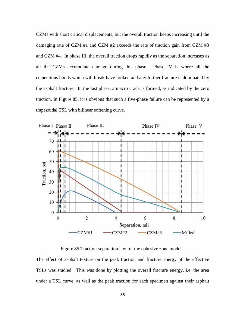
88

CZMs with short critical displacements, but the overall traction keeps increasing until the

damaging rate of CZM #1 and CZM #2 exceeds the rate of traction gain from CZM #3

and CZM #4. In phase III, the overall traction drops rapidly as the separation increases as

all the CZMs accumulate damage during this phase. Phase IV is where all the

cementious bonds which will break have broken and any further fracture is dominated by

the asphalt fracture. In the last phase, a macro crack is formed, as indicated by the zero

traction. In Figure 85, it is obvious that such a five-phase failure can be represented by a

trapezoidal TSL with bilinear softening curve.

Figure 85 Traction-separation law for the cohesive zone models.

The effect of asphalt texture on the peak traction and fracture energy of the effective

TSLs was studied. This was done by plotting the overall fracture energy, i.e. the area

under a TSL curve, as well as the peak traction for each specimen against their asphalt

89

roughness. Figure 86 shows no definite relation between the peak traction and the asphalt

roughness. However, the fracture energy increases with the HMA roughness. This agrees

with the previous conclusion based on Table 13 that milling resulted in a thicker ITZ

shifting the interfacial fracture into the asphalt but not increasing the peak traction. This

again implies that the bond strength is not a suitable parameter for evaluating the

effectiveness of milling.

Figure 86 Influence of the HMA roughness on the peak traction and fracture energy of

the cohesive elements.

The size effect of the WST was also studied. Figure 87 shows the relationship between

the fracture energy, as well as the peak strength, and the asphalt depth. For both milled

and unmilled specimens, a greater asphalt depth seems to relate to smaller fracture energy.

This is because the interfacial crack process zone is relatively small when the asphalt

thickness is large, which results in a more brittle failure that presents smaller fracture

energy. Similarly, there is a relatively large crack process zone when the asphalt is

Traction: y = 6.03x0.4

R² = 0.08

Energy: y = 0.0011x1.2

R² = 0.71

0

50

100

150

200

250

300

0

10

20

30

40

50

60

70

0 20 40 60 80

Fra

cture

ener

gy,

psi

.mil

Pea

k t

ract

ion,

psi

Roughness, mil

Traction Energy

90

milled or the asphalt is thin, resulting in larger fracture energy. There is no definite

correlation between the peak strength and the asphalt depth.

Figure 87 Influence of the asphalt depth on the peak traction and fracture energy of the

cohesive elements.

The peak traction as well as the fracture energy was plotted against the flaw size (initial

notch depth) in Figure 88. There is no clear evidence that the fracture energy is a

function of the initial flaw size. However, the peak traction shows an inversely

proportional relationship with the flaw size. In WST, the test configuration results in a

compression zone at the bottom of the interface. Since damage is unlikely to happen in

this compression zone, its upper bound defines the lower bound of the damage

developing zone. In the finite element model, it was observed that the size of this

compression zone was consistently 15-20% of the nominal contact area at the beginning

of the WST and it gradually diminished when the fracture approached the bottom of the

interface. Therefore, a deeper initial notch would result in a smaller damage developing

Traction: y = 5.3x1.0

R² = 0.07

Energy: y=1974x-2.5

R² = 0.55

0

50

100

150

200

250

300

0

10

20

30

40

50

60

0 1 2 3 4 5

Fra

cture

ener

gy,

psi

.mil

Pea

k t

ract

ion,

psi

Asphalt thickness, in

Traction-unmilled Energy-unmilled

Traction-milled Energy-milled

91

zone and thus a smaller peak traction force. On the other hand, the fracture energy is

dominated more by the thickness of the ITZ, not the depth of the damage developing

zone along the interface. In Figure 88, it is also noteworthy that the effect of the flaw

size almost disappears when the initial notch depth is less than 10%. Therefore, only the

specimens with initial notch of 10% or less should be used for the inverse analysis of

fracture properties for the CZMs.

Figure 88 Influence of the initial flaw size on the peak traction and fracture energy of the

cohesive elements.

3.6 Summary

In this chapter, a cohesive zone model based on the superimposition principle was used to

model the interfacial fracture of ultrathin whitetopping. Fractured UTW specimens were

first examined and four major types of failure were identified, namely the failure of

cement adhesion to asphalt matrix, the failure of cement adhesion to exposed/crushed

aggregate, aggregate breakage/pullout, and asphalt fracturing. Five root CZMs were

Traction: y = 3.84x-1.1

R² = 0.59 Energy: y = 115x0.1

R² = 0.006

0

50

100

150

200

250

300

0

10

20

30

40

50

60

70

0% 10% 20% 30% 40% 50%

Fra

cture

ener

gy,

psi

.mil

Pea

k t

ract

ion,

psi

Normalized notch depth

Traction Energy

92

proposed to represent the four types of failure. The complicated overall fracture behavior

of the interface can then be simulated by the superimposition of the root CZMs.

The fracture properties of the root CZMs were obtained based on the inverse analysis of

wedge splitting test results. The properties are material dependent and independent from

the composition of the interface, i.e. the milling effect, so that they can be used to model

the debonding of whitetopping on different scales.

In general, the overall CZM for UTW can be approximated by a trapezoidal traction-

separation law with bilinear softening. An analysis of the properties for the overall CZM

revealed that the peak traction decreases with increased initial notch depth until the initial

notch depth dropped to 10% or less of the nominal contact length. The total fracture

energy is a function of the asphalt roughness and asphalt thickness. A milled specimen

with thin asphalt often presents a relatively thicker interfacial transition zone and thus

results in fracture of the asphalt. Such type of fracture is less brittle and presents higher

fracture energy. However, scrutiny should be used when evaluating the asphalt

roughness due to milling, because no bond was observed where milling left deep grooves

into the asphalt. The deposit of debris and dust in these grooves breaks the bond and

more often there is no concrete setting into the grooves due to the small width-to-depth

ratio of such grooves.

93

REFERENCES

Alfano, M., F. Furgiuele, Leonardi, A., Maletta, C. and Paulino, G. H. (2009). Mode I

fracture of adhesive joints using tailored cohesive zone models. International Journal of

Fracture, Vol. 157, No. 1-2, pg.193-204.

Alfano, M., Furgiuele, F., Leonardi, A., Maletta, C., and Paulino, G. H. (2007). Cohesive

zone modeling of mode I fracture in adhesive bonded joints. Key Engineering Materials,

No. 348-349, pg. 13-16.

Al-Qadi, I. L., Carpenter, S. H., Leng, Z, Ozer, H. and Trepanier, J. S. (2008). Tack Coat

Optimization for HMA Overlays: Laboratory Testing. Research Report FHWA-ICT-08-

023, Illinois Center for Transportation.

ASTM-E965-96 (2006). Standard Test Method for Measuring Pavement Macrotexture

Depth Using a Volumetric Technique. Retrieved from www.astm.org, 2012.

ASTM C469. Standard Test Method for Static Modulus of Elasticity and Poisson's Ratio

of Concrete in Compression. Retrieved from www.astm.org, 2012.

AASHTO T 342-11. Standard Method of Test for Determining Dynamic Modulus of Hot-

Mix Asphalt Concrete Mixtures.

ABAQUS. ABAQUS Theory Manual (6.11).

Bazant, Z.P. and Becq-Giraudon E. (2002). Statistical prediction of fracture parameters of

concrete and implications for choice of testing standard, Cement and Concrete Research,

Vol. 32, pg. 529-556.

Brühwiler, E., & Wittmann, F. H. (1990). The Wedge Splitting Test, A New Method of

Performing Stable Fracture Mechanics Tests. Engineering Fracture Mechanics, 35(1-3),

117-125.

Chabot, A., Balay, J.M., Pouteau, B. and De Larrard, F. (2008). FABAC accelerated

loading test of bond between cement overlay and asphalt layers. Pavement Cracking –

Al-Qadi, Scarpas & Loizos (eds).

http://link.springer.com/search?facet-author=%22A.+Leonardi%22

http://link.springer.com/search?facet-author=%22C.+Maletta%22

http://link.springer.com/search?facet-author=%22G.+H.+Paulino%22

http://www.astm.org/

94

Delatte, N. and Sehdev, A. (2003). Mechanical properties and durability of BCO and

UTW concrete, Paper presented for the 82th TRB annual meeting Washington D.C.,

January, 2003.

Feraren, P. and Jensen, H. M. (2004). Cohesive zone modeling of interface fracture near

flaws in adhesive joints. Engineering Fracture Mechanics, Vol. 71, No., 15, pg. 2125-

2142.

Granju, J. L. (2004). Interface between an Old Concrete and a Bonded Overlay:

Debonding Mechanism, Interface Science, Vol. 12, pp. 381-388.

Guinea, G.V., Planas, J. and Elices, M. (1994). A general bilinear fitting for the softening

curve of concrete. Materials and Structures, Vol. 27, pg. 99–105.

Hillerborg, A., Modeer, M., and Petersson, P. E., (1976). Analysis of crack formation and

crack growth in concrete by means of fracture mechanics and finite elements. Cement

and. Concrete. Research, Vol. 6, No. 6, pg. 773–781.

Kim, H., Wagoner, M. P., and Buttlar, W. G. (2008). Simulation of fracture behavior in

asphalt concrete using a heterogeneous cohesive zone discrete element model. Journal of

Materials in Civil Engineering, Vol. 20, No. 8, pg. 552-563.

Kim, S.M. and Nelson, P. K. (2004). Experimental and numerical analyses of PCC

overlay on PCC slabs-on-grade subjected to climatic loading. International Journal of

Solids and Structures, 41, 785-800.

Li, S., Thouless, M. D., Waas, A.M., Schroeder, J.A., and Zavattieri, P.D. (2005). Use of

mode-I cohesive-zone models to describe the fracture of an adhesively-bonded polymer-

matrix composite. Composites Science and Technology, Vol. 65, No. 2, pg. 281-293.

Mohammed, I. and K. M. Liechti (2000). Cohesive zone modeling of crack nucleation at

bimaterial corners. Journal of the Mechanics and Physics of Solids, Vol. 48, No.4, pg.

735-764.

Park, K., Paulino, G. H., and Roesler, J. (2010). Cohesive fracture model for functionally

graded fiber reinforced concrete. Cement and Concrete Research, Vol. 40, No. 6, pg. 956-

965.




95

Pouteau, B., Balay, J.M., Chabot, A. and De-Larard, F. (2004). Faituge test and

mechanical study of adhesion between concrete and asphalt. 9th International

Symposium on Concrete Road, Istanbul, April 2004.

Song, S. H., Paulino, G. H., and Buttlar, W. G. (2008). Influence of the cohesive zone

model shape parameter on asphalt concrete fracture behavior. AIP Conference.

Tarr, S. M., M. Sheehan and P. A. Okamoto. (1998). Guidelines for the Thickness Design

of Bonded Whitetopping Pavement in the State of Colorado. Report No. CDOT-DTD-R-

98-10. Colorado Department of Transportation, Denver, CO.

Tvergaard, V. and Hutchinson J. W. (1992). The relation between crack-growth

resistance and fracture process parameters in elastic plastic solids. Journal of the

Mechanics and Physics of Solids, Vol. 40, No. 6, pg. 1377-1397.

Wu, C. L, S. M. Tarr, T. M. Refai, M. A. Nagi and M. J. Sheehan. (1999). Development

of Ultra-Thin Whitetopping Design Procedure. PCA Research and Development, Serial

No. 2124, Portland Cement Association, Skokie, IL.

Ural, A., Krishnan, V. R. and Papoulia (2009). A cohesive zone model for fatigue crack

growth allowing for crack retardation, International Journal of Solids and Structures, Vol.

46, No. 11-12, pg. 2453-2462.

Vandenbossche, J. M. and A. J. Fagerness. (2002). Performance, Analysis, and Repair of

Ultrathin and Thin Whitetopping at Minnesota Road Research Facility. Transportation

Research Record, Transportation Research Board, National Research Council,

Washington, DC. Vol.1809, pp. 191–198.

laboratory and numerical investigation of interface ... reinforced concr… · laboratory and...

Documents