laboratory course “industrial automation”
TRANSCRIPT
University of Stuttgart
Institute of Industrial Automation and Software Engineering Prof. Dr.-Ing. M. Weyrich
Room 2.146
Laboratory Course “Industrial Automation”
Experiment No. 2
Real-time programming with Ada
Experiment instructions
Real-time programming with Ada 2
Table of contents
1 INTRODUCTION ............................................................................................................ 4
1.1 WAYS OF REAL-TIME DATA PROCESSING ................................................................................................. 4 1.2 CONTENT AND PURPOSE OF THIS EXPERIMENT ......................................................................................... 4
2 THE ADA PROGRAMMING LANGUAGE ................................................................ 4
2.1 ORIGIN AND HISTORICAL OVERVIEW ....................................................................................................... 4 2.2 ADVANTAGES OF ADA............................................................................................................................. 5 2.3 STRUCTURE OF THE ADA PROGRAMMING LANGUAGE ............................................................................. 6
2.3.1 Formal structure of the programs ......................................................................... 6
2.3.2 Types .................................................................................................................... 6
2.3.3 Operators .............................................................................................................. 8
2.3.4 Commands in Ada ................................................................................................ 8
2.3.5 Program Units .................................................................................................... 10
3 SET-UP OF THE MPS PA COMPACT WORKSTATION ...................................... 13
4 STRUCTURE OF THE EXISTING ADA PROCESS CONTROLLER .................. 18
4.1 FIELD LEVEL .......................................................................................................................................... 18 4.1.1 Communications link level ................................................................................. 18
4.1.2 Communication command level ......................................................................... 19
4.1.3 Communication manager level ........................................................................... 19
4.1.4 Module interface level ........................................................................................ 19
4.2 PROCESS VARIABLE LEVEL .................................................................................................................... 19 4.2.1 Analog Interfaces ............................................................................................... 19
4.2.2 Digital interfaces ................................................................................................ 22
4.3 PROCESS CONTROL LEVEL ..................................................................................................................... 22 4.4 GRAPHICAL USER INTERFACE ............................................................................................................... 22 4.5 SCENARIO EXPERIMENT ......................................................................................................................... 22
4.5.1 Communication control ...................................................................................... 23
4.5.2 Analog input signals ........................................................................................... 23
4.5.3 Digital input signals ........................................................................................... 24
4.5.4 Analog output signals ......................................................................................... 24
4.5.5 Digital output signals ......................................................................................... 24
4.5.6 Experiment control ............................................................................................. 24
5 USER MANUAL ............................................................................................................ 24
5.1 POSSIBLE PROBLEMS DURING LAB EXPERIMENT .................................................................................... 25
6 SAMPLE PROJECT "AUTOMATION OF A BOTTLING PLANT" .................... 26
6.1 INTRODUCTION ...................................................................................................................................... 26 6.2 ASSIGNMENT OF TASKS ......................................................................................................................... 26
7 TASKS AND EXPERIMENTS ..................................................................................... 30
7.1 INSTRUCTIONS FOR EXPERIMENTAL PROCEDURE ................................................................................... 30 7.2 INTRODUCTION TASKS ........................................................................................................................... 30 7.3 IMPLEMENTATION OF THE STARTING POSITION AND EMERGENCY SWITCH FUNCTIONALITY .................. 32 7.4 IMPLEMENTATION OF THE TEMPERATURE CONTROL .............................................................................. 32

Real-time programming with Ada 3
8 LITERATURE ............................................................................................................... 33
9 APPENDIX ..................................................................................................................... 34

Real-time programming with Ada 4
1 Introduction
This laboratory provides an introduction to the Ada programming language and the
automation of a model bottling plant.
1.1 Ways of real-time data processing
The Monitoring and management of technical equipment in the industry is one of the main
topics and main task of automation technology. Without the ability to control and automate
complex technical processes our current life would not be possible to this extent especially in
our way of consumption of goods. What began with the invention of the first industrial fit
steam engine by Thomas Newcomen in 1712, was continued in 1913 with the introduction of
the first motorized assembly line by Henry Ford.
Of course nowadays a productions line not only consists of one assembly line, but can consist
of many machines with fast and precise movements that demand complex control
requirements. To be able to control and automate such a system, various computer systems
are used, which must handle process data in real-time very often, so that the system works
properly.
To handle process data in real-time, there can be used various options. The use of
Programmable logic controllers (PLC)
Hardware-related microprocessors und -controllers
High-level programming in conjunction with a real-time operating system on a PC
Programming using real-time programming language (e.g. Ada)
are approved methods.
The advantages of Ada for real-time operation are, for example, parallel processing of tasks,
time-controlled behavior and exclusive access to resources. Thereby with Ada it is possible to
perform real-time programming directly, without being dependent on interfaces of a real-time
operating system.
1.2 Content and purpose of this experiment
A typical task of an automation engineer is to develop a real-time system. This experiment
serves to provide an insight into the programming of such real-time systems using the Ada
programming language. For this purpose on the one hand a sample program has to be
expanded and on the second hand there has to be realized an automation for a bottling plant.
Therefor a model of an industrial bottling plant from Festo Didactic is used, the MPS PA
Compact-Workstation.
In order to ensure a rapid and successful experiment execution, the experiment must be
thoroughly prepared. For that purpose the complete manual must be read including the
appendix and the preparation tasks of Chapter 6 are to be processed in written form before the
execution of the experiment.
2 The Ada programming language
2.1 Origin and historical overview
Ada was developed in the 1970s. At this time the U.S. Department of Defense (DoD)
prompted an internal investigation and found out that more than 450 different programming

Real-time programming with Ada 5
languages have been used in their projects. To reduce the enormous effort that was necessary
to maintain the used software, a task force was established. The aim of this task force was to
standardize and list the requirements of the DoD. Despite the many programming languages
available on the market, none of them could meet the requirements in the area of maintenance,
training, modularity and reuse. After a global request of bids, the concept of Jean Ichbiah
(language standard ANSI/MIL-STD-1815A 1983) was chosen and called Ada831. In the
following years Ada has been revised, expanded and standardized by the ANSI (American
National Standards Institute) and the ISO (International Organization for Standardization).
With the expansion of object-oriented features, Ada95 (language standard ANSI/ISO/IEC-
8652: 1995) became the first standardized object-oriented programming language.
In order to promote the rapid spread of the language, the U.S. Departement of Defense
directed till 1997 that in all software projects of the DoD at least 30% of the code had to be
implemented in Ada. In addition, the GNAT compiler was funded by the U.S. Air Force and
provided free of charge to all users.
2.2 Advantages of Ada
Nowadays Ada is widely-used in security-critical areas of real-time reference, for example, in
the military. The reasons for this are plentiful.
On the one hand, Ada was standardized very strictly and the entire standard has been
available for free ever since, in the so-called Ada Language Reference Manual. In addition all
Ada compilers have to run through extensive tests and accomplish those correctly if they want
to be officially validated. This leads to a high portability on other systems.
The code is checked already at compile time to detect, for example, slips of the pen directly
and to ensure the formal correctness. This reduces considerable the effort of quality assurance.
In addition, a run-time check is performed so that an error is triggered when violations of
predefined rules arise. This feature of Ada is called the exception handling. This allows to
prescribe how the program should react in case of an error, for example, display a specific
error code or to bring the plant to a safe state. Besides, this will make it much easier to
localize the error. Since Ada was developed for very large and complex systems with millions
of lines of code, this feature is also a guarantee that Ada is so widespread in safety-critical
task areas such as air traffic control, weapon systems, or in the aerospace.
Another advantage of Ada is the possibility to divide a software project in different modules.
This is one reason why very large and complex software projects are being realizable with
Ada. Furthermore, the modularity simplifies the understanding of the program and minimizes
the effort to expand it. Through the use of libraries and thus the use of already established
lines of code the expansion of programs is greatly simplified and accelerated.
The ability to manipulate individual bits and to program at register level makes Ada even
interesting for the low-level hardware programming.
Other advantages are [IAS07]:
Support of methods of software engineering
Support for reusability
Event-driven and concurrent programming
Use of a program library
Interface to peripheral software systems
Object orientation with dynamic polymorphism
Real-time support
1 after the British mathematician Ada Lovelace (1815-1852)

Real-time programming with Ada 6
Optional automatic garbage collection
Parallel processing
2.3 Structure of the Ada programming language
2.3.1 Formal structure of the programs
The character set of an Ada program consists of the 26 basic letters of the Latin alphabet in
upper and lower case. Although umlauts are possible, it is strongly recommended to set those
aside if you want to develop software with international use. To the basic letters, all digits
from 0 to 9, space and the following characters are added: " # ' ( ) * + , - . / : ; < = > _ | & [ ] { }
All lexical units consist of this character set. There are identifiers, reserved words, numeric
literals, character literals, string literals, delimiters, and comments. A Space between two
lexical items is ignored by Ada.
Identifiers for program components, variables, etc. begin with a letter. After that, any number
of letters, digits and underscores can follow. However, underscores are not allowed to succeed
and they cannot be at the end of the identifier. In addition, an identifier may go up to the end
of line at the most. For better readability, identifiers are to be preferred which are as short and
concise as possible. Ada distinction is generally not case-sensitive, however identifiers should
be written consistent over all parts of the program, as otherwise the compiler could complain.
The following keywords are reserved in Ada and cannot be used as identifiers:
abort begin else goto new private reverse until abs body elsif not procedure use abstract end if null protected select accept case entry in separate when access constant exception is of raise subtype while aliased exit or range with all declare limited others record tagged and delay for loop out rem task xor array delta function renames terminate at digits mod packages requeue then do generic pragma return type
For numeric literals Ada granted some freedoms. In this representation of integers, for
example, underscores can be inserted to improve readability. 1_500_000 or 1.5e6 correspond
to the numerical value 1500000. Furthermore, any number can be provided to a basis between
2 and 16. The numerical value 15 in decimal notation corresponds to the numerical value of
16#F in hexadecimal and to 2#1111 in binary notation. As decimal separator Ada uses a
point.
Character literals (character) may consist of any character and be enclosed by quotation marks
('Z'). String literals (strings), however, may also consist of none character (empty string) and
be enclosed by double quotes ("String").
Delimiter (delimiter) can be used individually or assembled (compound delimiter) and include
the following characters: ' ( ) * + , - . / : ; < = > | &
The last thing to mention here are comments. These are characterized by a double hyphen and
go till the end of the line (-- this would be a comment).
2.3.2 Types
With types, the programmer has the opportunity to submit its own container values. One type
is for example the enumeration: type month is (January, February, .. December);.
Real-time programming with Ada 7
2.3.2.1 Integers
For the representation of integers, the type „integer“ is used in Ada. Furthermore, there is the
type of "positive" for all numbers greater than zero and type "natural" for all numbers greater
than or equal to zero. Here a special feature of Ada is that you can specify your own value
ranges. In this case we speak of a subtype. If for example you do not need the full range of an
integer, you can specify a smaller range of values2. To declare a value range of 0 to 10, you
write: subtype smaller_range is integer range 0 .. 10;.
If you want to calculate with multiple integers of different value ranges, an automatic type
conversion takes place. If a suitable conversion cannot be preformed, a “constraint_error” is
triggered.
Example: X=5 has a value range of 0 .. 10 and Y=10 has a value range of 0 .. 20. Now if the
expression X+Y is calculated and written back to Y, everything is fine (Y=15). However, if
this expression is being calculated and written back to X a “constraint_error” occurs because
the range of values of X is not sufficient.
Should the value of a variable not be changeable, you add a „constant“ in front of the type
(e.g. number_months: constant integer := 12;).
2.3.2.2 Real Numbers
Real numbers can be specified in Ada as floating-point, fixed-point or decimal numbers.
For floating point numbers the exact decimal places must be declared and you can also
specify a range of values: type length is digits 2; (e.g. 10.55), type percent is digits 4 range
0.0 .. 1.0; (e.g. 0.3456).
For fixed-point numbers, the difference between two successive values must be specified.
Analogous to floating-point numbers, it is optionally also possible to specify a range of
values: type length is delta 0.01;.
To conclude, there is the possibility to declare real numbers as decimal numbers. Here, both,
the difference and the decimal places need to be indicated: type temperature is delta 0.01
digits 2;.
2.3.2.3 Arrays
When declaring arrays, you have the possibility to determine the exact bounds of the array
(constrained array) or leave them open (unconstrained array): type Eight_Bit is array(0 .. 7)
of boolean; (constrained array), type Vector is array(integer < >) of positive; (unconstrained
array).
In the definition of constrained arrays you do not need to specify the boundaries: Byte:
Eight_Bit;. But in case of a unconstraint array you have to specify the boundaries: Square:
Matrix(1 .. 5, 1 .. 5);.
In order to access a single element of an array, you use parentheses: Byte(3), Square(2, 4). In
addition you can also cut out (slices) a selected range from an array and receive a new array:
Byte(3 .. 6).
2.3.2.4 Private (abstract) types
To protect specific components of an object from possibly accidental change, Ada is
providing the private types: type day is private;. Those must be declared twice in the package
specification. First, it must be described incompletely in the public block (before the keyword
„private“). I.e. you declare for example that a variable is private (type X is private;).
Secondly, this type must then be fully described in the non-visible part (type X is range -10 ..
10;).
2 With Ada the initiator decides which value range of an integer is used, depending on the available hardware.
But at least the range from -32 768 to +32 767 (16-bit)

Real-time programming with Ada 8
2.3.3 Operators
Similar to other programming languages, in Ada there are different operators. The most
important are listed here:
** potentiate = equality
abs() absolute value /= inequality
not negation <; <= less than, less than or equal
* multiplication >; >= greater, greater than or equal
/ division and conjunction
+ addition or disjunction
- subtraction xor exclusive disjunction
As another operator there has to be noted the binary operator „&“ which joins two strings
(one-dimensional arrays).
2.3.4 Commands in Ada
In Ada three different commands are distinguished. Agreement, expression and statement. In
the following, the three types are briefly described.
2.3.4.1 Agreements
Agreements declare variables or subroutines. Basically, you specify the name, followed by the
type and possibly a starting value: X: integer := 17;. Here the container value „X“ was
declared as a type „integer“ with the initial value 17.
2.3.4.2 Expressions
Expressions calculate a value, but it typically does not change content of containers. Thus, for
example: 10 + X * 4 is an expression that calculates a value based on the content of the
container "X".
2.3.4.3 Statements
Unlike expressions, statements can change the content of a container value and must be
terminated by a semicolon. This is most evident in the assignment statement: X := X + Y + 5;.
Here an expression is calculated and its result is written back into the container value "X". It
should be noted that, for example, the screen and the keyboard are also count as container
values and therefore input and output commands are statements as well.
In the following, additional important statements are presented.
2.3.4.3.1 The null statement
The null statement is described by "null;" and serves the purpose of doing nothing. This is
often useful as a placeholder for future functionalities.
2.3.4.3.2 The if and case statement
The if and case statement is being used for selection. Here the
programmer has the possibility that a statement may not be executed.
With loops in contrast, he can achieve that a statement is called
multiple times. The basic structure is shown in Figure 1.
The if statement can also contain any number of elsif branches, but
must not have an else call necessarily.
In the case statement, the expression must either belong to the type
integer or enumeration. In addition, the value of the expression must
be known already at compile time, not at run time. Furthermore a case Figure 1 - Basic structure
of if and case statement

Real-time programming with Ada 9
statement must be fully and clearly. If completeness cannot be reached you have to use
„others“ as last entry.
2.3.4.3.3 The exit statement
To exit loops there is the unconditional and conditional exit statement: exit;, exit when
Expression;. On demand, you can also specify the loop name after the key word „exit“: exit
loop_name when X=Y;. If the exit statement is before any other statement in the loop, it is a
pre-checking loop. Is it behind all other statements in the loop, it is a post-checking loop.
2.3.4.3.4 Loops
Loops are divided into three different types.
There is a loop without iteration, a while and a for loop. Furthermore, the loop without
iteration is used to simulate loop types
that do not actually exist in Ada (e.g. pre-
and post- checking until loop). While it is
possible that a loop or while loop become
an infinite loop, this danger does not
appear with a for loop.
For loops can run through the entire range
of values of the variable type, or only a
limited range of values with the keyword
„range“. If it is necessary to run through
the loop parameter in descending order
instead of ascending order (default), there
is the keyword „in reverse“.
Loops can also be named by writing the
name with a colon before the loop block.
This makes it possible that you always
know exactly which loop is ending or
being left, even with nested loops. Figure 2 shows the basic structure of the loops above.
2.3.4.3.5 The block statement
The block statement is divided into a declaration part and a
statement part. The basic structure is shown in figure 3. The
declaration part is initiated by „declare“ and ends with „begin“,
where the statement part begins. This is terminated by „end“. The
block statement creates the container values declared in the
declaration part and then executes the statements. When exiting the
block statement, all container values created are getting cleared. If
not needed, the declaration part can be omitted. If you want to
name the block, you put the name followed by a colon either before „declare“ (with
declarations), or before „begin“ (without declarations).
2.3.4.3.6 The return statement
To exit subroutines and jump back to the origin of the call you use the return statement.
Within procedures you only use the keyword „return“ with a final semicolon. For functions
the calculated expression must be given back to the origin of the call: return Expression;.
Figure 2 - Basic structure of loops
Figure 3 - Basic structure
of the block statement

Real-time programming with Ada 10
2.3.4.3.7 The raise statement
With the raise statement you trigger the exception handling. Ada provides a run-time
monitoring and triggers special predefined exceptions (constraint_error, programm_error,
etc.), even without the raise
statement by the programmer.
For example, when divided
by 0.
However, the programmer
may declare and define own
exceptions and define how to
proceed when this exception
occurs. In addition, he can
also access the exceptions
already defined by Ada and
trigger those without having
to implement them.
Exceptions are declared in the
declaration part and raised in
the statement part. If you want to call a particular statement with one exception, you can use
the exception handler for this purpose. To describe this, an exception part is inserted at the
end of the statement part by using the keyword „exception“. This part ends with the keyword
„end“ then. Now you can specify what should be done when an exception occurs.
To illustrate the impact of an exception, we briefly assume that a procedure or similar is a
framework.
If now an exception is raised in the code section of an inner frame, the initiator goes from
normal state into the state of emergency. Here, it jumps to the exception part of the inner
frame and looks for the name of the raised exception. If the right exception handler is found, it
executes its instructions, then goes back to normal state and terminates the inner frame. Now,
the outer frame is being continued at the point after the inner frame.
If there is no matching exception handler, the initiator will remain in state of emergency and
terminates the inner frame. After that it triggers the same exception again in the outer frame
and jumps into the exception part. Now it looks for the appropriate exception handler again
and proceeds analog to the inner frame.
Is there again no matching exception handler and there is no more additional outer frame, the
entire program will be aborted with an error message. The basic structure of exception
handling is shown in Figure 4.
2.3.5 Program Units
There are basically four different units in Ada.
Subroutines
Tasks
Reusable libraries (packages)
Shared resources (protected variable)
Program units are usually divided into a specification file (file extension .ads) and an
implementation file (file extension .adb). The specification file must not be present in order to
compile an executable program. But it is strongly recommended to use this useful feature of
Ada for an easy understanding of programs. In the specification file, all necessary
informations to call a program unit is stored (name, parameter, parameter type, parameter
mode, etc.). It should also include a comment to briefly describe what this program unit does
Figure 4 - Basic structure of exception handling in a procedure

Real-time programming with Ada 11
exactly. A specification is usually much clearer and easier to understand than a complex
implementation. In the implementation file, first the specifications are repeated and thereafter
the instructions are formulated.
2.3.5.1 Subroutines
Subroutines are statements or expressions, which are combined in a block and assigned with a
name. This way you can use it multiple times without having to insert the code all over again.
In addition this simplifies the understanding and maintenance of the software, as well as the
readability.
Subroutines are divided into two parts. At the beginning there is the declaration with the
name, parameters and if it is a function, the return value is also defined. The second part is the
implementation of the instructions.
A distinction is made here, on the one hand the library subroutines that can be called from
anywhere and on the other hand the contained subroutines, which can only be called within
the unit in which they are described.
Figure 5 shows an example of a contained subroutine.
Here the procedure “Main” is a library subroutine and the
procedure “Under” is in “Main” included and can only be
called within that procedure. The fact should be noted that
the lines 2 - 5 only generate the procedure “Under” and do
not execute it. In line 8 this procedure finally is executed
explicitly. For this purpose, it must be called with its name
and terminated by a semicolon.
When a subroutine is called, it executes its instructions in
order. If the keyword „return“ is used, the subroutine is
terminated at this point and it will jump back to the place
from where the subroutine was called.
There are two different types of subroutines. Procedures and functions.
The main difference is that a call of a procedure corresponds to a statement and returns no
value (e.g. put; get; etc.). In this case container values can be changed. The call of a function
corresponds to an expression and returns a value (e.g. +; -; <; <=; etc.). In this case values are
calculated but no container values are changed.
2.3.5.1.1 Procedure
A procedure can contain (any number of) parameters in 3 different modes. The basic
structure is shown in Figure 6. A distinction is made here, parameters, which are transported
from the calling point to the procedure (keyword „in“ or without keyword), parameters, which
are transported from the procedure to the calling point (keyword „out“) and parameters which
are used for both ways
(keyword „in out“).
An in parameter (any
expression) is passed
from the calling point
to the subroutine and is
treated by that as a
constant. An out parameter (name of a variable) corresponds to an uninitialized variable and is
written in the subroutine and then is passed to the calling point. An in-out parameter (name of
a variable) behaves like an initialized variable. So the subroutine gets a variable with an initial
value. It is allowed to read this variable, overwrite it with a new value and then gives it back
to the calling point.
Figure 6 - Basic structure of a procedure with parameters
Figure 5 - Example of a subroutine
Real-time programming with Ada 12
2.3.5.1.2 Function
A function can only have in parameters and must have at least one return statement. Thereby,
the return value is specified, which will be returned to the calling point by that function:
return sum;.
2.3.5.2 Tasks
With tasks it is possible in Ada to work through command sequences not only sequentially
but also parallel. Fundamentally an Ada program is executed in one main task. The
programmer has the possibility to define more tasks, which are then executed side by side and
next to the main task. A subroutine can be executed at the same time as part of different tasks.
Tasks are also separated into specification part and body and must be specified. A task that
has been declared in the declaration section of a program unit is started just before the
execution of the instructions in this program unit, but only after all agreements have been
processed.
2.3.5.2.1 Delay statements
In order that tasks do not directly run after calling a program, there are the delay statements.
Firstly, there is the delay statement, which causes the task to be paused for the specified time
(in seconds) (delay 5.0; --task is paused 5 seconds).However, it can only be guaranteed here
that the task is stopped for this period. Whether the task starts again immediately afterwards,
cannot be guaranteed because another task could be running at that time. Secondly, there is
the delay until statement. In contrast to the relative time specifyed by the delay statement, the
delay until statement provides an absolute time: delay until time;.
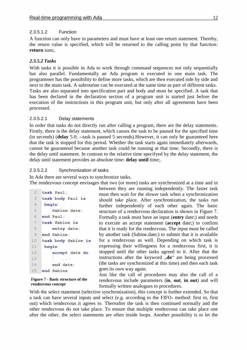
2.3.5.2.2 Synchronization of tasks
In Ada there are several ways to synchronize tasks.
The rendezvous concept envisages that two (or more) tasks are synchronized at a time and in
between they are running independently. The faster task
must then wait for the slower task when a synchronization
should take place. After synchronization, the tasks run
further independently of each other again. The basic
structure of a rendezvous declaration is shown in Figure 7.
Formally a task must have an input (entry date;) and needs
to execute an accept statement (accept date;) to confirm
that it is ready for the rendezvous. The input must be called
by another task (Sabine.date;) to submit that it is available
for a rendezvous as well. Depending on which task is
expressing their willingness for a rendezvous first, it is
stopped until the other tasks agreed to it. After that the
instructions after the keyword „do“ are being processed
(the tasks are synchronized at this time) and then each task
goes its own way again.
Just like the call of procedures may also the call of a
rendezvous include parameters (in, out, in out) and will
formally written analogues to procedures.
With the select statement (selective synchronization), this concept is further extended. So that
a task can have several inputs and select (e.g. according to the FIFO- method: first in, first
out) which rendezvous it agrees to. Thereafter the task is then continued normally and the
other rendezvous do not take place. To ensure that multiple rendezvous can take place one
after the other, the select statements are often inside loops. Another possibility is to let the
Figure 7 - Basic structure of the
rendezvous concept
Real-time programming with Ada 13
task only wait a certain time for a rendezvous with a delay statement. If the rendezvous does
not take place within this period, the task performs an alternative sequence of statements.
Another method to synchronize tasks is to use protected variables. Even protected objects
have a specification part and a body (similar to a package). The specification here consists of
a visible and an invisible (private) part. Here, all variables must be declared as „private“. So
you have no way to access those variables from the outside and you need to use the
procedures within the resource, since only those have access rights to the variables.
If multiple tasks simultaneously access a protected object and try to read it, this is possible
without any problems. Write access is allowed only in sequence and is monitored by the
initiator.
2.3.5.3 Reusable libraries (packages)
Packages are used to group several subroutines, but may also include types and objects. It
may be useful or necessary, that parts of an existing program are being reused. To ensure that
this part is functional even without the rest of the program, all necessary subroutines and
agreements are combined into one package. Such a package is then easy to integrate and also
allows development of the program with several mutually independent programmers.
Packages even make it possible to use a variable that is needed in various subroutines to use
as a "global" variable and to prevent the deletion by the subroutine after its execution
(variable remains exist with its value).
Such a package consists similar to a subroutine of a specification part (package specification:
package name is .. end name;) and an implementation part (package body: package body
name is .. end name;). These units can also be translated separately. The agreements, which
are described in the package body are not visible outside of the package. A package is not
executable alone. For this purpose, a subroutine is needed, which calls the program units and
variables from the package. To this end however, the package must be included first. To do
so, you use the keyword “with” followed by the name of the package in the first line of the
file. If the keyword “use” with the package name is following, all routines of the package are
accessible without having to call them with “packagename.procedurename”.
3 Set-up of the MPS PA Compact Workstation
Festo Didactic develops industry-related education and training systems to meet the growing
educational demands of the industry. Since it is financially and technically often hardly
possible to shut down industrial plants for education and training of the own employees,
models of these systems are needed to provide an understanding of the individual processes
and dependencies. These are developed and if necessary supervised by Festo Didactic.
One of these models, the MPS PA Compact Workstation is shown in Figure 8.

Real-time programming with Ada 14
Figure 8 - MPS PA Compact-Workstation by Festo Didactic
This workstation is a model of an industrial-related bottling plant and is a learning system for
a variety of regulation and control tasks. It has four integrated control loops that can be
operated individually by manually switching the ball valves. This guarantees a very high
complexity in the smallest space. The level, flow, pressure and temperature control loop allow
a wide-ranging coverage of industrial automation tasks and the connection with various
technologies such as pneumatic process actuators ensure a strong practical relevance. The
industry is using pneumatic actuators for valves more and more since they have clear
advantages in terms of safety and energy efficiency. The combination of various technologies
in automation technology becomes more and more important.
The Compact Workstation provides tasks in the areas of:
Mechanics
Process control
Pneumatic / Compressed air technology
Sensors / actuators
PLC
Closed loop control systems
Closed loop control
Fault finding
The system combines pneumatic, hydraulic and electrical components.
Figure 9 shows the P&I diagram (piping and instrumentation diagram) of the bottling plant:

Real-time programming with Ada 15
Tank102
Tank101
V112
V187 M
V110
V102
S
S115
V103
V106
P101
B102
FIC
V104
V105
V108
V107
VSSL103
V101
B103
PIC
E104 B104
TIC
S111
LSH
B113
LSL
S117
S112
B114
LSH
Sensor_Level_Tank_B101
B101
LIC
Pressure_Tank_B103
Proportional_Valve_V106
Pump_P101
Heating_Tank_101
FloatSwitch
Temperature_Tank_B104
Proximity_Switch_Min_Level_B113
Proximity_Switch_Max_Level_B114
Float_Switch_S111
Flow_Meter_Pump_B102
Float_Switch_S112
Figure 9 - P&I diagram
The components of the system, which allow an interaction are now mentioned and described
based on figure 9:
The main components are the two large tanks (tank 101, tank 102) which are connected to
each other through various pipes. Here, several control loops can be activated and deactivated
by manually opening or closing the ball valves.
Furthermore, the model has several analog and digital sensors and some actuators.
The sensors provide all necessary information about the system and communicate via the
communication module EasyPortUSB with the control program. Since a USB connection can
only transmit digital values, the EasyPortUSB module transmits the analog measured values
(0 to 10V) in a 12-bit resolution, i.e. discrete values from 0 to 4095. This information must
then be converted into the right analog values by the software. Here, the EasyPort only serves
as a transfer interface between the software and the system and assumes no technical control
functions. Only the sensor information from the system is being transferred to the software
and the controlling commands are being passed to the actuators.
The plant has four analog sensors.
Analog sensors [Garc12]:
B101 [Level sensor tank 102]
ID Sensor_Level_Tank_B101
Sensor type Ultrasonic sensor
Description The sensor is located at the top of the tank 101, and measures the distance up to the water surface. Thus the filling level is determined. (Tank full: 10V; tank empty:

Real-time programming with Ada 16
0V).
measuring range
Distance (50 - 345mm)
Output Voltage (10 - 0V DC)
B102 [flow rate sensor]
ID Flow_Meter_Pump_B102
Sensor type Flow rate sensor
Description The sensor is located directly behind the pump and measures the water flow rate through the pipe.
measuring range
Flow rate (0,3 - 9,0l/min)
Output Frequency (40 - 1200Hz)
Flow rate sensor measuring transducer [Frequency to Voltage]
ID f/U
Sensor type Measuring transducer frequency to voltage
Description The measuring transducer converts the displayed frequency by the flow rate sensor into a voltage signal.
measuring range
Frequency (0 - 1kHz)
Output Voltage (0 - 10V DC)
B103 [Pressure sensor]
ID Pressure_Tank_B103
Sensor type Pressure sensor
Description The sensor measures the water pressure in the pipes which is generated by the pump and the proportional valve (V106).
measuring range
Pressure (0 - 400mbar)
Output Voltage (0 - 10V DC)
B104 [PT100 Temperature sensor]
ID Temperature_Tank_B104
Sensor type Temperature sensor
Description The sensor measures the water temperature in tank 101.
measuring range
Temperature (0 - 100°C)
Output Voltage (0 - 10V DC)
The communication module EasyPortUSB also supports 16 digital inputs and outputs. In the
system, following digital sensors are used.
Digital sensors [Garc12] (Output: boolean: true/false):
B102 [Flow rate sensor]
ID Flow_Meter_B102
Description This signal is used with a high-speed counter for measuring the frequency.

Real-time programming with Ada 17
S111 [Float switch]
ID Float_Switch_S111
Description Maximum filling level of tank 101.
S112 [Float switch]
ID Float_Switch_S112
Description Middle filling level of tank 102.
B113 [Capacitive proximity switch]
ID Proximity_Switch_Min_Level_B113
Description Minimum filling level of tank 101. The heater cannot be used from here.
B114 [Capacitive proximity switch]
ID Proximity_Switch_Max_Level_B114
Description Maximum filling level of tank 101. Ball valve must be closed.
S115 [Ball valve closed]
ID Ball_Valve_Closed_S115
Description Ball valve is closed.
S116 [Ball valve opened]
ID Ball_Valve_Open_S116
Description Ball valve is opened.
In addition, the plant has four actuators.
Actuators [Garc12]:
V102 [Ball valve with pneumatic actuator]
ID Ball_Valve_V102
Typ Ball valve with pneumatic actuator
Description The valve controls the flow rate from tank 102 into tank 101.
Control Digital signal to open or close the valve.
101 [Heater tank 101]
ID Heating_Tank_101
Typ Heater
Description The heater heats the water in tank 101 if the fluid level is not too low.
Control Digital signal to turn the heater on and off.
P101 [Pump]
ID Pump_P101
Typ Pump
Description The pump can be operated in a analog or digital mode.
Control Pump_P101_Preset_D_A: Selection signal between analog and digital mode. Pump_P101: In the digital operating mode, the pump is turned on and off by this signal. Pump_P101_Analog: In analog mode, this signal controls the output level of the pump.
Real-time programming with Ada 18
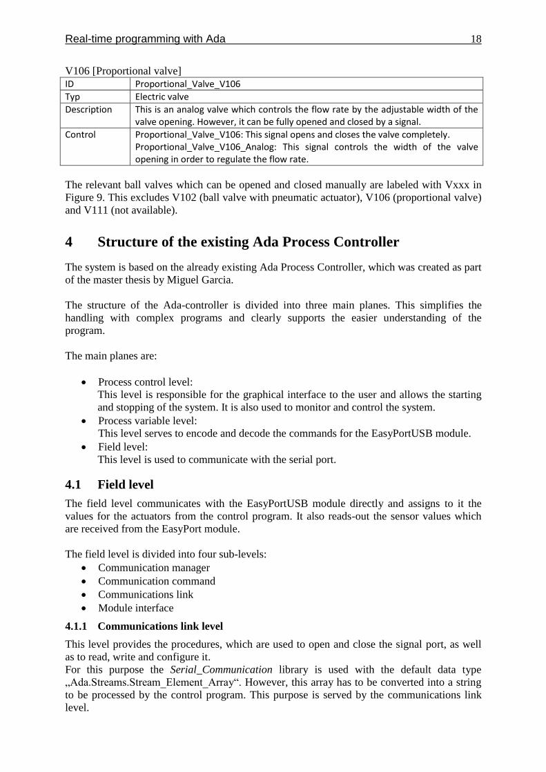
V106 [Proportional valve]
ID Proportional_Valve_V106
Typ Electric valve
Description This is an analog valve which controls the flow rate by the adjustable width of the valve opening. However, it can be fully opened and closed by a signal.
Control Proportional_Valve_V106: This signal opens and closes the valve completely. Proportional_Valve_V106_Analog: This signal controls the width of the valve opening in order to regulate the flow rate.
The relevant ball valves which can be opened and closed manually are labeled with Vxxx in
Figure 9. This excludes V102 (ball valve with pneumatic actuator), V106 (proportional valve)
and V111 (not available).
4 Structure of the existing Ada Process Controller
The system is based on the already existing Ada Process Controller, which was created as part
of the master thesis by Miguel Garcia.
The structure of the Ada-controller is divided into three main planes. This simplifies the
handling with complex programs and clearly supports the easier understanding of the
program.
The main planes are:
Process control level:
This level is responsible for the graphical interface to the user and allows the starting
and stopping of the system. It is also used to monitor and control the system.
Process variable level:
This level serves to encode and decode the commands for the EasyPortUSB module.
Field level:
This level is used to communicate with the serial port.
4.1 Field level
The field level communicates with the EasyPortUSB module directly and assigns to it the
values for the actuators from the control program. It also reads-out the sensor values which
are received from the EasyPort module.
The field level is divided into four sub-levels:
Communication manager
Communication command
Communications link
Module interface
4.1.1 Communications link level
This level provides the procedures, which are used to open and close the signal port, as well
as to read, write and configure it.
For this purpose the Serial_Communication library is used with the default data type
„Ada.Streams.Stream_Element_Array“. However, this array has to be converted into a string
to be processed by the control program. This purpose is served by the communications link
level.

Real-time programming with Ada 19
The main procedures are ReadMessage, SendMessage and InitConnectPort.
The procedure ReadMessage reads-out the port and saves it in a string.
The procedure SendMessage transmits the information to the serial port.
The procedure InitConnectPort initializes and configures the port.
4.1.2 Communication command level
This level describes the functions and procedures to communicate with the EasyPortUSB
module.
Two types of procedures are basically used here. One type reads the information from the
module and the other transmits information to the module.
The function ReadI uses the special command to read the input and returns the
decoded value (from hex to decimal).
The procedure WriteO writes the output in hexadecimal system.
Additional there is a procedure ConfigSetup.
The procedure ConfigSetup reads the address of the EasyPort and checks the
correctness of the answer. To allow communication at first this message is sent to the
EasyPort.
4.1.3 Communication manager level
The communication manager level provides the procedures to read the inputs from the
EasyPort and pass the outputs to the EasyPort. Three procedures are used therefor.
The procedure InitCommunications creates a new object of type EasyPort and then
enables communication with the EasyPort. Only after this procedure has been called,
the communication with the EasyPort is possible. This procedure also allows you to
connect and communicate with multiple EasyPortUSB modules.
The procedure UpdateInputs reads-out all the inputs of all EasyPorts and stores them
in the respective object.
The procedure UpdateOutputs transmits all outputs to the EasyPort module.
4.1.4 Module interface level
The module interface level provides the functions and procedures, which are necessary for the
conversion of the inputs and outputs.
4.2 Process variable level
The process variable level is used to convert the raw data from the sensors into useful
information and to encode the commands for the outputs and output them in the range of the
EasyPort.
4.2.1 Analog Interfaces
The EasyPortUSB module supports four analog inputs and two analog outputs in a value
range of either 0V DC to 10V DC or -10V DC to +10 V DC. For digital transmission of this
information the EasyPort uses a range of values from 0 to 4095 discrete values, this
corresponds to a resolution of 12bit. In this system always a value range of the sensors from
0V DC to 10V DC is used.
The formulas for converting between the desired voltage and the raw data and vice versa are
the following [Garc12]:
𝑣𝑜𝑙𝑡𝑎𝑔𝑒 =raw data
4095∗ 10
raw data =voltage
10∗ 4095

Real-time programming with Ada 20
4.2.1.1 Level sensor B101 [Garc12]:
ID Sensor_Level_Tank_B101
Sensor type Ultrasonic sensor
Description The sensor is located at the top of tank 102, and measures the distance to the surface of the water. Thus the filling level is determined. (Tank full: 10V; Tank empty: 0V).
measuring range
Distance (50 - 345mm)
Output Voltage (10 - 0V DC)
Connection Analog Input 1
Function Sensor_Level_Tank_B101.get
Filling level = (12𝑙
340𝑚𝑚) ∗ ((
345𝑚𝑚 − 50𝑚𝑚
4095) ∗ 𝑟𝑎𝑤 𝑑𝑎𝑡𝑎 + 50)
4.2.1.2 Flow rate sensor [Garc12]:
ID Flow_Meter_Pump_B102
Sensor type Flow rate sensor
Description The sensor is located directly behind the pump and measures the water flow through the pipe.
measuring range
Flow rate (0,3 - 9,0l/min)
Output Frequency (40 - 1200Hz)
ID f/U
Sensor type Measuring transducer frequency to voltage
Description The measuring transducer converts the frequency given by the flow rate sensor into a voltage signal.
measuring range
Frequency (0 - 1kHz)
Output Voltage (0 - 10V DC)
Connection Analog Input 2
Function Flow_Meter_Pump_B102.get
𝐹𝑙𝑜𝑤 𝑟𝑎𝑡𝑒 = 𝑟𝑎𝑤 𝑑𝑎𝑡𝑎 ∗ (10𝑉
4095) ∗ (
1𝑘𝐻𝑧
10𝑉) ∗ (
9𝑙
𝑚𝑖𝑛1,2𝑘𝐻𝑧
)
4.2.1.3 Pressure sensor [Garc12]:
ID Pressure_Tank_B103
Sensor type Pressure sensor
Description The sensor measures the water pressure in the pipes, which is generated by the pump and the proportional valve (V106). The sensor is located behind the pump.
measuring range
Pressure (0 - 400mbar)
Output Voltage (0 - 10V DC)
Connection Analog Input 4
Function Pressure_Tank_B103.get

Real-time programming with Ada 21
𝑃𝑟𝑒𝑠𝑠𝑢𝑟𝑒 = 𝑟𝑎𝑤 𝑑𝑎𝑡𝑎 ∗ (10𝑉
4095) ∗ (
400𝑚𝑏𝑎𝑟
10𝑉)
4.2.1.4 Temperature sensor [Garc12]:
ID Temperature_Tank_B104
Sensor type Temperature sensor
Description The sensor measures the water temperature in tank 101.
measuring range
Temperature (0 - 100°C)
Output Voltage (0 - 10V DC)
Connection Analog Input 3
Function Temperature_Tank_B104.get
𝑇𝑒𝑚𝑝𝑒𝑟𝑎𝑡𝑢𝑒𝑟 = 𝑟𝑎𝑤 𝑑𝑎𝑡𝑎 ∗ (10𝑉
4095) ∗ (
100°𝐶
10𝑉)
4.2.1.5 Pump [Garc12]:
ID Pump_P101
Type Pump
Description The pump can be operated in an analog or digital mode.
Steuerung Pump_P101_Preset_D_A: Selection signal between analog and digital mode. Pump_P101: In digital mode of operation, the pump is turned on and off by this signal. Pump_P101_Analog: In analog mode, this signal controls the output level of the pump.
Maximale Leistung
Flow rate 10l/min
Input Voltage (0 - 10V DC)
Connection Analog Output 1
Function Pump_P101_Analog.set()
𝑅𝑎𝑤 𝑑𝑎𝑡𝑎 = 𝑝𝑒𝑟𝑐𝑒𝑛𝑡 ∗ (4095
100)
4.2.1.6 Proportional valve [Garc12]:
ID Proportional_Valve_V106
Type Electric valve
Description This is an analog valve which controls the flow rate by the variable width of the valve opening. However, it can be fully opened and closed by a signal.
Steuerung Proportional_Valve_V106: This signal opens and closes the valve completely. Proportional_Valve_V106_Analog: This signal controls the width of the valve opening in order to regulate the flow rate.
Maximaler Wert
Flow rate 10l/min
Input Voltage (0 - 10V DC)
Connection Analog Output 2
Function Proportional_Valve_V106_Analog.set()
𝑅𝑎𝑤 𝑑𝑎𝑡𝑎 = 𝑝𝑒𝑟𝑐𝑒𝑛𝑡 ∗ (4095
100)
Real-time programming with Ada 22
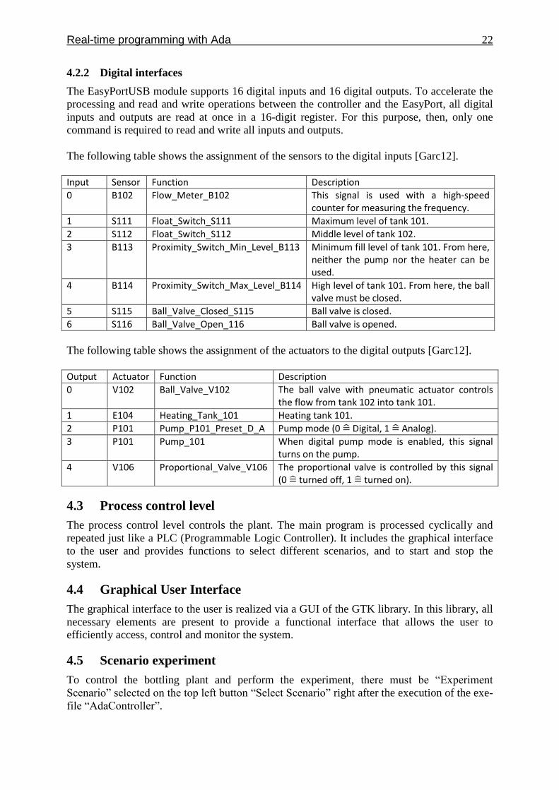
4.2.2 Digital interfaces
The EasyPortUSB module supports 16 digital inputs and 16 digital outputs. To accelerate the
processing and read and write operations between the controller and the EasyPort, all digital
inputs and outputs are read at once in a 16-digit register. For this purpose, then, only one
command is required to read and write all inputs and outputs.
The following table shows the assignment of the sensors to the digital inputs [Garc12].
Input Sensor Function Description
0 B102 Flow_Meter_B102 This signal is used with a high-speed counter for measuring the frequency.
1 S111 Float_Switch_S111 Maximum level of tank 101.
2 S112 Float_Switch_S112 Middle level of tank 102.
3 B113 Proximity_Switch_Min_Level_B113 Minimum fill level of tank 101. From here, neither the pump nor the heater can be used.
4 B114 Proximity_Switch_Max_Level_B114 High level of tank 101. From here, the ball valve must be closed.
5 S115 Ball_Valve_Closed_S115 Ball valve is closed.
6 S116 Ball_Valve_Open_116 Ball valve is opened.
The following table shows the assignment of the actuators to the digital outputs [Garc12].
Output Actuator Function Description
0 V102 Ball_Valve_V102 The ball valve with pneumatic actuator controls the flow from tank 102 into tank 101.
1 E104 Heating_Tank_101 Heating tank 101.
2 P101 Pump_P101_Preset_D_A Pump mode (0 =̂ Digital, 1 =̂ Analog).
3 P101 Pump_101 When digital pump mode is enabled, this signal turns on the pump.
4 V106 Proportional_Valve_V106 The proportional valve is controlled by this signal (0 =̂ turned off, 1 =̂ turned on).
4.3 Process control level
The process control level controls the plant. The main program is processed cyclically and
repeated just like a PLC (Programmable Logic Controller). It includes the graphical interface
to the user and provides functions to select different scenarios, and to start and stop the
system.
4.4 Graphical User Interface
The graphical interface to the user is realized via a GUI of the GTK library. In this library, all
necessary elements are present to provide a functional interface that allows the user to
efficiently access, control and monitor the system.
4.5 Scenario experiment
To control the bottling plant and perform the experiment, there must be “Experiment
Scenario” selected on the top left button “Select Scenario” right after the execution of the exe-
file “AdaController”.
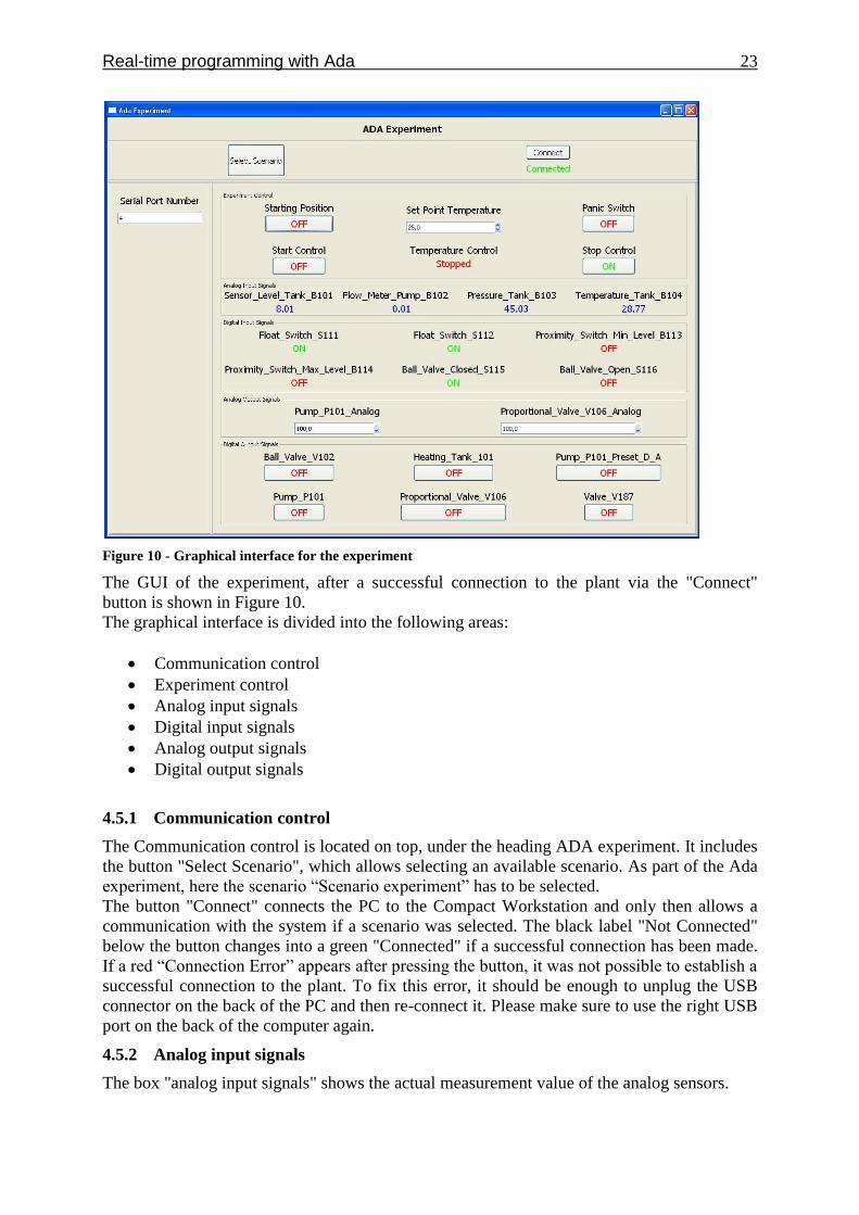
Real-time programming with Ada 23
Figure 10 - Graphical interface for the experiment
The GUI of the experiment, after a successful connection to the plant via the "Connect"
button is shown in Figure 10.
The graphical interface is divided into the following areas:
Communication control
Experiment control
Analog input signals
Digital input signals
Analog output signals
Digital output signals
4.5.1 Communication control
The Communication control is located on top, under the heading ADA experiment. It includes
the button "Select Scenario", which allows selecting an available scenario. As part of the Ada
experiment, here the scenario “Scenario experiment” has to be selected.
The button "Connect" connects the PC to the Compact Workstation and only then allows a
communication with the system if a scenario was selected. The black label "Not Connected"
below the button changes into a green "Connected" if a successful connection has been made.
If a red “Connection Error” appears after pressing the button, it was not possible to establish a
successful connection to the plant. To fix this error, it should be enough to unplug the USB
connector on the back of the PC and then re-connect it. Please make sure to use the right USB
port on the back of the computer again.
4.5.2 Analog input signals
The box "analog input signals" shows the actual measurement value of the analog sensors.

Real-time programming with Ada 24
4.5.3 Digital input signals
The box "digital input signals" indicates the current state of the digital sensors.
4.5.4 Analog output signals
The box “analog output signals” allows the input of an analog value for controlling the analog
actuators pump (P101) and proportional valve (V106).
4.5.5 Digital output signals
The box “digital output signals” allows the point-and-click control of the digital actuators
heating (Heating_Tank_101) as well as the turning on and off of the pump and the
proportional valve. Furthermore, here can be switched between the analog and digital mode of
the pump.
4.5.6 Experiment control
The upper box "Experiment Control" allows the control of the experiment.
The button "Starting Position" creates the desired initial state. This means that the valve V102
is closed and the liquid level of tank 101 is right below sensor B113 (so B113 is off).
The button “Panic Switch” has the function of an emergency stop switch, which is usually
common for every system in the industry. It is implemented in software, and converts the
system in any operating state to a safe state immediately. This means that every actuator
(pump, heater and valves) is turned off. After pressing the emergency switch though the
further use of the system is possible without any restrictions.
In the middle you can set the desired temperature for the temperature control in a range
between 20°C .. 30°C and the label underneath the caption “Temperature Control” gives
colored feedback if the temperature control is active (green “Running”) or inactive (red
“Stopped”).
To be able to press the “Start Control” button, at first it is necessary to establish the initial
state, otherwise the button is without function.
The "Stop Control" button interrupts the automation program in each phase and restores the
initial state. After pressing the “Stop Control” button though the further use of the system is
possible without any restrictions.
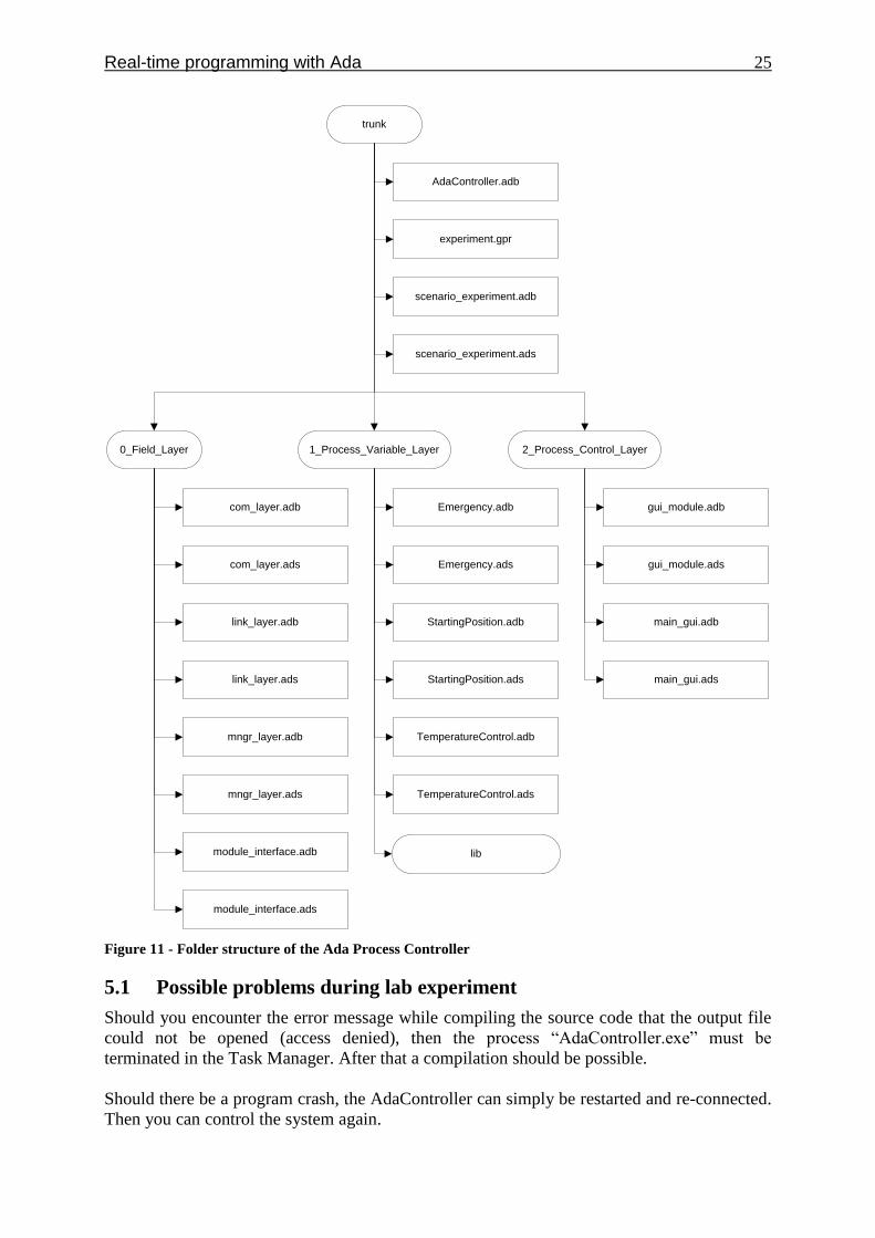
5 User manual
Figure 11 shows the folder structure of the Ada Process Controller. To create the executable
exe file with the project file "experiment.gpr", this structure must be maintained.
With the command “gnatmake -Pexperiment” in the command prompt, the code is compiled
and the executable file “AdaController” is created.
Real-time programming with Ada 25
trunk
0_Field_Layer 1_Process_Variable_Layer 2_Process_Control_Layer
gui_module.adb
gui_module.ads
main_gui.adb
main_gui.ads
Emergency.adb
Emergency.ads
StartingPosition.adb
StartingPosition.ads
TemperatureControl.adb
TemperatureControl.ads
com_layer.adb
com_layer.ads
link_layer.adb
link_layer.ads
mngr_layer.adb
mngr_layer.ads
module_interface.adb
module_interface.ads
AdaController.adb
experiment.gpr
scenario_experiment.adb
scenario_experiment.ads
lib
Figure 11 - Folder structure of the Ada Process Controller
5.1 Possible problems during lab experiment
Should you encounter the error message while compiling the source code that the output file
could not be opened (access denied), then the process “AdaController.exe” must be
terminated in the Task Manager. After that a compilation should be possible.
Should there be a program crash, the AdaController can simply be restarted and re-connected.
Then you can control the system again.

Real-time programming with Ada 26
If it is not possible to make a successful connection to the plant, then the USB connector on
the back of the PC has to get unplugged and re-connected. After that it should be possible to
re-establish a connection to the plant. It should be noted that the USB port (Port 4) is
maintained.
6 Sample project "Automation of a bottling plant"
6.1 Introduction
The CEO of a chemical bottling company has the following problem. Recent researches have
shown that certain chemicals can be excreted if the temperature of the liquid is too low and
the holding time in the filling tank is too long. These chemicals settle in the tank and cause a
reduction of the chemical concentration of the filled liquid on the one hand. On the other
hand, a dangerously high concentration in the liquid can occur if the tank gets refilled and
turbulences ensure that the deposit in the tank gets combined with the liquid again. The filling
process represents the end of the production line and the quality control takes place right
before the filling tank. Consequently, there is no monitoring unit to check the chemical
concentration of the liquid directly before bottling.
At a proper operation of the system, the dwell time of the liquid in the filling tank is too short
so that the described phenomenon will not take place. However, the duration increases in case
of an error somewhere in the production line. If the process has to be interrupted, then the
concentration of the liquid could change. Since the purchasers of the liquids can accept almost
no tolerance for concentration variation and the TÜV discovered this problem at a routine
check, the CEO has to act fast.
Either an expensive monitoring system for the filling tank has to be installed, which does not
prepare the existing liquid in a case of an error, or there has to be found another solution to
keep the liquid at a certain temperature in the case of an error.
If this problem is not resolved in the shortest possible time, the company is threatened by the
closure of the plant with an unforeseeable financial damage.
To save time and money, the CEO decides to use the alternative of a temperature control.
You now have the task as a software developer to implement this and other functions.
6.2 Assignment of tasks
Since there only exists an in hardware realized emergency stop switch for the plant, you
should first develop an emergency stop switch realized in software for the plant.
Firstly,we need to establish the “starting position” and further extend it to perform
temperature control functionality.
Moreover, in order to avoid deposits of a liquid in tank 102, the fluid must be brought to a
certain temperature and maintained. For this purpose you should develop a temperature
control. Since it is not possible to integrate a heater in tank 102, the CEO decides to reactivate
a unused tank with heater. Fortunately, the tanks have already been connected to each other
by a piping system. The CEO envisages the system in case of an error in the following way:
The liquid which is stored in tank 102 has to be dumped gradually through the electric valve
V102 into the re-activated tank 101. There the liquid has to be brought to a certain
temperature. Once the temperature has reached the setpoint, the heater is switched off and the
liquid gets pumped back into tank 102. This process should continue until the fault has been
eliminated. After that the initial state must be restored. With that the control program is over.
The following requirements are placed on the automation:

Real-time programming with Ada 27
The emergency stop switch has to switch off all actuators at any time.The main
functionality of the emergency stop is that we should be able to stop the process of
automation at any point of time. When the emergency switch is pressed, the entire
plant comes to a stop.
Setpoint for the temperature of the liquid should be 23°C
The automation needs to be terminated by the “Stop Control” button at any time.When
“stop control “ is pressed, the plant reverts back to it’s starting position.
. It is important to establish the starting position in order to check for temperature
control.
Realization of the emergency stop switch:
To realize the emergency stop switch, at first the file Emergency.adb must be implemented.
The corresponding specification file is located in the Appendix.
The emergency stop switch should be realized as exception within the procedure
“PanicSwitch”.
The emergency stop switch must convert the plant to a safe state at any time. This means:
The temperature control must be stopped
The valve Ball_Valve_V102 must be closed
The pump Pump_P101 must be switched off
The pump preset is to be set to false
The proportional valve Proportional_Valve_V106 must be closed
The heater Heating_Tank_101 must be switched off
After pressing the emergency stop switch it should be possible to control the full system
further. Therefore all required variables must be meaningfully overwritten. It is recommended
that after the outputs are coded and updated to perform a delay statement (500ms) and then to
finish the statement block by overwriting the variable "Panic_Switch_Hit".
Realization of the initial state:
Since the Compact Workstation is a model, first there needs to be a sensible initial state
created to run the temperature control then. For this, the file StartingPosition.adb must be
implemented. The corresponding specification file is located in the Appendix.
The starting position means that the Ball_Valve_V102 is closed and the level of the water in
tank 101 is just below the sensor B113. On the one hand it should be able for the user to
activate it via the button “Starting Position”. Another situation where the initial state can be
restored is when the “stop contol” feature of temperature control module is activated.Before
the initial position can be prepared first it needs to be checked whether there is too little liquid
in the tank 101 at the beginning. Only then can the loop "Starting Position" for the initial
position can be executed.
If the level in tank 101 is below sensor B113, the variable “Low_Level_Tank_101” is to be
assigned true. Otherwise, the variable should get the value false as well as the variable
“Start_Created”.
Sequence:
If the initial position is not already established, the loop “StartingPosition” is to be started.
First, the inputs are updated and decoded.
If the level in tank 101 (Low_Level_Tank_101) is too low, the procedure “FillingTank” first
opens the Ball_Valve_V102 and then codes and updates the outputs.
In the following loop “FillingLoop” only the inputs are updated and decoded, followed by a
short waiting interval of 200ms. The loop “FillingLoop” should be left as soon as the sensor
B113 is active.
Real-time programming with Ada 28
After that the procedure “StopFillingTank” (structurally identical to “FillingTank”) must
close the valve V102. Now the low level at the beginning has been corrected and the actual
initial position can be prepared.
For this purpose, at first it is ensured again by the procedure “CreateStart”, that the valve
V102 is closed. Subsequently the proportional directional valve V106 is fully opened. For this
purpose, at first the analog value must be set and then the valve V106 must be opened. Only
then the pump is turned on.
Finally, the outputs should be coded and updated.
There now follows a loop "StartingLoop" which is constructed identically to the loop
"FillingLoop". It should be left as soon as the level is below the sensor B113.
In conclusion of loop “StartingPosition” the pump and then the proportional directional valve
V106 need to be turned off by the procedure “StopStart”. And then the outputs need to be
encoded and updated.
Finally the required variables need to be overwritten then. Now the procedure “StopStart” is
completed and the initial position is prepared.
Note that it must be able to bring the plant in a safe condition by pressing the emergency stop
switch at all times.
Realization of the automation program:
For testing purposes, the case of an error in chapter 6.1 should be triggered by the user using
the button “Start Control” in the GUI. Thereby the temperature control ("RunningLoop") is
activated, but only if the starting position was created.
After triggering the error, at first the inputs are updated and decoded.
Then the current level of tank 102 is read with the procedure "StartSetLevel" and the desired
level (1.5 liters less) is determined. Thereafter, the valve V102 is opened and the outputs
encoded and updated.
The following loop "LevelLoop" is of the same structure as "FillingLoop". It is to be exited as
soon as the desired level is reached.
Afterwards, the valve V102 must be closed by means of the procedure "StopSetLevel" and the
outputs must be encoded and updated.
After repeated updating and decoding of the inputs, the set temperature for the temperature
control is read with the command "SetPoint_Temperature:=
Float(get_value(Set_Point_Spinner));".
With the procedure "SetTemperature", the current temperature is only read and assigned to
the variable "Current Temperature".
Now, if the current temperature is lower than the set temperature, the heating should be turned
on by means of the procedure "StartHeating" with subsequent encoding and updating of the
outputs.The following loop "TemperatureLoop" is identical to the loop "FillingLoop" and
should be exited once the desired temperature has been reached.
Now the heating must be turned off again with the procedure "StopHeating" (structurally
identical to "StartHeating").
Before there will be a waiting interval of 1s now there should be the possibility to exit the
loop "RunningLoop" with the buttons "Stop Control" or "Panic Switch". Do not forget that
this must be possible at any time of the temperature control.
After waiting that one second, the initial position should get restored and the loop
"RunningLoop" should be exited.
Further notes:
The complete program of this experiment is running within a task in
scenario_experiment.adb. All loops are to be implemented in this task. See the corresponding
excerpt in the Appendix.

Real-time programming with Ada 29
Starting position
Close Valve V187
Turn off Pump
P101
Start Created
Analog value
V106 := 100.0
Open Valve V106
Turn on Pump
P101
B113 = true?
yes
no
Close Valve V106
Low_Level_Ta
nk_101=true?Open Valve V187yes B113 = false?
yes
no no
Start Control
Level higher
than
StopLevel?
Close valve V187
no
yes
Temperature
less than
setpoint?
Stop Heating
Start Heating
Set Current
Temperature
Temperature
less than
setpoint?
yes
no
no
yes
Create starting
position
SetStartLevel
SetStopLevel
Open Valve V187
Read SetPoint
Temperature
The packages Emergency, StartingPosition and TemperatureControl should only be used to
control actuators and to overwrite variables, so that the program remains clear in the
scenario_experiment file. Stick to the respective specification files concretely. Here all
required methods with parameters are described. Also do not forget that all these parameters
must be used to ensure proper operation. This is for learning purposes to give you an
understanding of modularity and parameter handling and exceptions in Ada.
Note that if you control actuators, you must encode and update the outputs, so that the
commands are passed to the system. You have to deal with the inputs similarly to obtain the
current value (update inputs and decode). These methods are already available and can be
used. See appendix.
In Figures 12 and 13, the respective flow diagrams for the initial sate and the temperature
control are shown.
Note: The flow charts represent only the main functions and are not complete.
For detailed description of the individual parts of the program, stick to chapter 6.2.
Figure 12 - Flow diagram starting position Figure 13 - Flow diagram temperature control

Real-time programming with Ada 30
7 Tasks and experiments
7.1 Instructions for experimental procedure
The main purpose of this experiment is to implement the automation program, which was
described in Chapter 6. The hardwarenear control of the system has been already realized and
is not part of the task of this experiment. All program units that are used to obtain and process
sensor data and to control actuators are already available and can be used. These are attached
in the appendix and must be worked through before experimental procedure. It must not be
converted any raw data. The level sensor returns a value in liters.
The experiment is performed on the Compact Workstation presented in chapter 3. As a
process computer there is a PC with Windows 8 provided. For the Ada programming the
program Notepad++ is used. Please save all files you edit exclusively in your group folder.
The Windows command prompt is used to compile source code. At the command prompt, you
must first navigate to drive C. To do so type C: and press enter. You may enter it by typing
cmd in the search box of the Windows start menu. To navigate in different folders in the
command prompt the command cd is used (cd foldername to navigate into the subfolder
“foldername” in the current folder; cd.. to navigate to the parent folder). Now to compile a file
use the command gnatmake programname for a single file, the command gnatmake -
Pprojectname for a project. To execute a program, only the program name must be called
from the command prompt in the specific folder.
To ensure that the experiment can be usefully and quickly processed, the instructions must be
read completely and the following tasks are to be processed in writing prior the experiment. In
addition, results have to be recorded during the experiment.
Notes about the plant: The valve V105 must be closed at any time. To be able to perform the
experiment properly, please ensure the following before the experiment and fill out the
checklist:
Ventil V101 is closed
Ventil V103 is closed
Ventil V104 is closed
Ventil V105 is closed
Ventil V107 is opened
Ventil V108 is opened
Ventil V110 is opened
Ventil V112 is closed
7.2 Introduction tasks
Preparation task 1: Expiration of task programs
a) Once all the agreements of a program have been processed, all tasks which are
declared within it and the main task are started (the main program itself is executed as
a task as well). Then all tasks are running in any order independently from each other.
This order can happen to be the same with a renewed program execution or may not
be. Now, however, a particular sequence is often required. What possibilities does the
programmer have with Ada to keep a specific order and how can he prevent an
uncontrolled start of the task at startup? Give an example of a task agreement and a
task body.

Real-time programming with Ada 31
b) As soon as a task has completed its instruction part, it is terminated. It is now no
longer possible to call this task except by restarting the main program. But often a
multiple execution of a task during a program is needed. What option is available to
execute a task several times? Give an example of such a task body.
Preparation task 2: Cyclic task programs and parameter passing
Automation technology often requires the use of cyclic processes (e.g. sampling control).
Additionally, it is often necessary that parameters are passed between task programs to read,
for example, sensor data once and further process somewhere else. The following example
program "Dating" illustrates the operation of parameter passing and synchronization between
tasks using the rendezvous concept.
In addition to the main program, four additional tasks are implemented. Eva, Dirk, Paul and
John. Dirk, Paul and John send Eva a rendezvous request named "Request" and pass it a
parameter of type String called "Gift". Eva now checks whether the "Gift" is "Flowers" and
refers this task on its own private entrance "Rendezvous". Is it not “Flowers” Eva then
dispenses that she does not like the “Gift”.
a) The Task Eva therefore has two entrences. A public entrence "Request" and a private
entrance "Rendezvous". Both entrences accept a parameter called "Gift" of type
String. Now create the specification of the task Eva and the other required tasks. Note
the specification file Dating.ads available in the appendix.
Note: To implement a private entrance, the keyword “private” is used. Here one or
more private entrences are included by “private” and “end task_name;”.
b) The Task Dirk performs first a delay statement (2s) like the two other tasks Paul and
John. After that, the task should either synchronize itself with Eva and, in this case
pass the parameter “Gift” which “Flowers” got assigned to, or if task Eva is still not
ready for synchronization after 10s, Dirk should perform an alternative statement
(Here it is the output „Dirk: I do not want to wait any longer, bye.“). The tasks Paul
and John do not perform an alternative statement block. The assigned parameters are
Paul: "Bread and butter", John: "Boot polish". Create the body of the tasks Dirk, Paul
and John in their prepared areas.
Note: In the declaration part TIO is declared as an abbreviation for Ada.Text_IO and
can be used analogously (Example: TIO.Put_Line („Hallo.“);.
c) The body of the task Eva is now to be finally created. Within a for loop, the three
synchronization requests should be processed. After a delay instruction (1s) was
executed the task Eva should accept and process the synchronization requests. In this
case an if branch is used. If the parameter "Gift" contains the string "Flowers", this
task is passed to the private entrance („requeue Entrancename with abort;“ the
addition „with abort“ allows task Eva to terminate itself, even if the synchronization
is not happening. This prevents a permanent waiting of task Eva and therefore also of
the complete program “dating”). If the Parameter should not be "Flowers", a further
delay statement (1s) is executed, followed by the output "Eva: Sorry, but I don‘t like "
&Gift& ".". Now follows another delay statement (1s) and the output is "Eva: I made
my decision." Now the synchronization request which was diverted to the private
entrance should in a subsequent select statement either be accepted and after a further
delay (1s) the output should be "Eva: Thank you for " &Gift& ". Let's go." or there
will be a delay of 5s with the output "Eva: I should have made up my mind faster.".
Create the body of task Eva.

Real-time programming with Ada 32
Experiment 1: Complete the Ada program "Dating" of Preparation Task 2 and produce the
output shown in Figure
14. Next, change the delay
statement after the for
loop from 1s to 10s in the
body of task Eva and run
the program again. Give
reasons for the result.
7.3 Implementation of the starting position and emergency switch
functionality
Preparation task 3: In order to use all functionalities several variables have to be declared.
List all required variables and set reasonable starting values if necessary. Only those variables
are required which are used as parameters, plus one, which is designated in the flowchart.
Note: A total of 10 variables are required of which one is already in place. Note the files
available in the appendix.
Preparation task 4: Design the emergency stop switch according to chapter 6. For this
purpose create the file Emergency.adb. Note the specification file Emergency.ads available in
the appendix.
Preparation task 5: Design the function "Starting Position". For this purpose create the file
StartingPosition.adb and the specific part in the scenario_experiment.adb. Note the
specification file StartingPosition.ads available in the Appendix. The starting position must be
designed in accordance to figure 12.
Experiment 2: Implement the designed program parts of the preparation tasks 3-5. First test
the functionality of the emergency stop switch by opening the valve Ball_Valve_V102 and
then press the emergency stop switch. Now check that the correct starting position is produced
by pressing the "Starting Position" button. Now drain some water and test the emergency stop
button while the starting position is creating for correct functionality.
7.4 Implementation of the temperature control
Preparation task 6: Design the control program temperature control from chapter 6. For this
purpose create the file TemperatureControl.adb and the specific part in the
scenario_experiment.adb. Note the specification file TemperatureControl.ads available in the
Appendix. The temperature control must be designed in accordance to figure 13.
Experiment 3: Implement the designed automation program of the preparation task 6. Test
your program with the help of the scenario "Scenario experiment".
First create the starting position by activating the button “Starting Position”. After the starting
position is established, you can trigger an error and start the temperature control, by pressing
the "Start Control" button. Now wait at least two cycles and then press the "Stop Control"
button. Now the starting position should be restored. Now check whether each of the
emergency stop button and stop switch for each phase (drain water, heat water, restore
starting position) yields the desired result. Make a check list for the possible options to verify
your results.
Note: The checklist should represent a table with 2 rows and 3 columns. It is then sufficient to
confirm the result with a check.
Figure 14 - Output of the example program „Dating“
Real-time programming with Ada 33
8 Literature
[AXE12] AXE: Ada Reference Manual, ISO/IEC 8652:2012(E) Language and Standard
Libraries. 3. Aufl., AXE Consultans, 2012.
[Blie98] Blieberger, J.: Rendezvous mit Ada Eine echtzeitige Annäherung. TU Wien,
http://www.auto.tuwien.ac.at/~blieb/ADA-Skriptum_TeX/gesamt/node9.html,
1998.
[Fest] Festo: MPS PA Datenblätter. Festo Didactic.
[Fest09] Festo: Prozessautomation und Regelungstechnik. Festo Didactic, 2009
[Fest13] Festo: MPS PA Compact- Workstation. Festo Didactic, http://www.festo-
didactic.com/de-de/lernsysteme/prozessautomation,regelungstechnik/compact-
workstation/mps-pa-compact-workstation-messen,steuern-und-regeln-auf-
kleinstem-raum.htm?fbid=ZGUuZGUuNTQ0LjEzLjE4Ljg4Mi43NjQ3, 2013.
[Garc12] Garcia, M.: Concept and realization of a process control for a bottling plant in
Ada. Masterarbeit, IAS, 2012.
[Göhn10] Göhner, P.: Automatisierungstechnik I, Vorlesungsskript Sommersemester 2010.
IAS, 2010.
[Grud01] Grude, U,: Einführung in Ada Ada95- Skript. TFH Berlin, http://public.tfh-
berlin.de/~grude/SkriptAda.pdf, 2001.
[Hube01] Huber, Steffen: Die Programmiersprache Ada. http://www.huber-
net.de/adagag.htm, 2001.
[IAS07] IAS: Versuch Nr. 2 Echtzeitprogrammierung mit Ada95 Versuchsanleitung. IAS,
2007.

Real-time programming with Ada 34
9 Appendix
--------------------------------------------------------------------------------------
-- File: Dating.ads
-- Project: Example program Dating
-- Author: Chris Brand
--
-- Main unit of Example program Dating
--------------------------------------------------------------------------------------
with Ada.Text_IO;
procedure Dating is
task Eva is
entry Request (Gift : string); --Task call with parameter called "Gift" of type
string.
private
entry Rendezvous (Gift : string); --private task call; for other tasks not
visible/accessible.
end Eva;
task Dirk;
task Paul;
task John;
end Dating;
--------------------------------------------------------------------------------------
-- File: Dating.adb
-- Project: Example program Dating
-- Author: Chris Brand
--
-- Main unit of Example program Dating
--------------------------------------------------------------------------------------
with Ada.Text_IO;
procedure Dating is
--------------------------------------------------------------------------------
package TIO renames Ada.Text_IO; --TIO is used as an abbreviation. Useful for programs
with many integrated libraries instead of "use".
--------------------------------------------------------------------------------
-- Task specifications --
--------------------------------------------------------------------------------
-- Body of task Eva --
task body Eva is
begin
delay 2.0;
TIO.Put_Line ("Eva is waiting for requests...");
end Eva;

Real-time programming with Ada 35
--------------------------------------------------------------------------------
-- Body of task Dirk --
--------------------------------------------------------------------------------
-- Body of task Paul --
--------------------------------------------------------------------------------
-- Body of task John --
--------------------------------------------------------------------------------
begin
delay 1.0;
TIO.Put_Line ("Dirk, Paul and John vie for the attention of Eva...");
end dating;
--------------------------------------------------------------------------------------
-- File: Emergency.ads
-- Project: Temperature Control
-- Author: Chris Brand
--
-- Unit of Panic Switch
--------------------------------------------------------------------------------------
package Emergency is
procedure PanicSwitch (Create_Start: in out Boolean; Start_Created: in out Boolean;
Running: in out Boolean; PreviousState_Running: in out Boolean; Panic_Switch_Hit:
in out Boolean);
end;
--------------------------------------------------------------------------------------
-- File: StartingPosition.ads
-- Project: Temperature Control
-- Author: Chris Brand
--
-- Unit of Starting Position
--------------------------------------------------------------------------------------
package StartingPosition is
procedure FillingTank;
procedure StopFillingTank;
procedure CreateStart;
procedure StopStart(Create_Start: in out Boolean; Start_Created: in out Boolean);
end;
--------------------------------------------------------------------------------------
-- File: TemperatureControl.ads
-- Project: Temperature Control
-- Author: Chris Brand
--

Real-time programming with Ada 36
-- Unit of Temperature Control
--------------------------------------------------------------------------------------
package TemperatureControl is
procedure StartSetLevel(Start_Level_Tank_102: in out Float; Stop_Level_Tank_102: out
Float);
procedure StopSetLevel;
procedure SetTemperature(Current_Temperature: in out Float);
procedure StartHeating;
procedure StopHeating;
end;
--------------------------------------------------------------------------------------
-- File: scenario_experiment.adb
-- Project: Experiment
-- Author: Chris Brand
--
-- Main unit for experiment
--------------------------------------------------------------------------------------
--------------------------------------------------------------------------------------
-- following package import area must not be modified by students --
--------------------------------------------------------------------------------------
...
with Emergency; use Emergency;
with StartingPosition; use StartingPosition;
with TemperatureControl; use TemperatureControl;
------------------------------------
-- end package import area --
------------------------------------
package body scenario_experiment is
type Controller_Experiment_Pointer is access Controller_Experiment;
---------------------------------------------------------------------
-- beginning declaration area for experiment variables --
---------------------------------------------------------------------
Starting_Position_Boolean : Boolean := False;
--------------------------------------------------
-- end declaration area for experiment --
--------------------------------------------------
...
---------------------------------------------------------------------------------------
-- beginning experiment buttons, must not be modified by students --
---------------------------------------------------------------------------------------
-- this procedure gets activated by pressing the button Panic Switch

Real-time programming with Ada 37
procedure Panic_Switch_Clicked (Widget : access Gtk_Widget_Record'Class) is
begin
Panic_Switch_Hit := true;
Set_Markup (Temperature_Control_L,("<span weight=""light""
color=""red"" size=""xx-large"">Stopped</span>"));
Emergency.PanicSwitch(Create_Start, Start_Created, Running,
PreviousState_Running, Panic_Switch_Hit);
end Panic_Switch_Clicked;
-- this procedure gets activated by pressing the button Starting Position
procedure Starting_Position_Clicked (Widget : access Gtk_Widget_Record'Class) is
begin
Create_Start := True;
end Starting_Position_Clicked;
-- this procedure gets activated by pressing the button Start Control
procedure Start_Control_Clicked (Widget : access Gtk_Widget_Record'Class) is
begin
if not (Task_Controller = null) then
if Start_Created = true then
Set_Markup (Temperature_Control_L,("<span weight=""light""
color=""green"" size=""xx-large"">Running</span>"));
Running := True;
PreviousState_Running := True;
end if;
end if;
end Start_Control_Clicked;
-- this procedure gets activated by pressing the button Stop Control
procedure Stop_Control_Clicked (Widget : access Gtk_Widget_Record'Class) is
begin
if not (Task_Controller = null) then
Set_Markup (Temperature_Control_L,("<span weight=""light""
color=""red"" size=""xx-large"">Stopped</span>"));
Running := False;
if PreviousState_Running = true and Panic_Switch_Hit = false then
Create_Start := true;
end if;
end if;
end Stop_Control_Clicked;
------------------------------------
-- end experiment buttons --
------------------------------------
...
----------------------------------------------------------------
-- beginning of programming area for experiment --
----------------------------------------------------------------
task body Controller_Experiment is
-- temperature used as set point with initial value 23.0°C (possible range 20.0°C till 30.0°C)
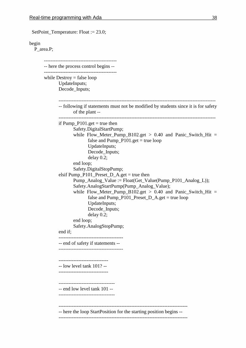
Real-time programming with Ada 38
SetPoint_Temperature: Float := 23.0;
begin
P_area.P;
--------------------------------------------
-- here the process control begins --
--------------------------------------------
while Destroy = false loop
UpdateInputs;
Decode_Inputs;
-----------------------------------------------------------------------------------------------
-- following if statements must not be modified by students since it is for safety
of the plant --
-----------------------------------------------------------------------------------------------
if Pump_P101.get = true then
Safety.DigitalStartPump;
while Flow_Meter_Pump_B102.get > 0.40 and Panic_Switch_Hit =
false and Pump_P101.get = true loop
UpdateInputs;
Decode_Inputs;
delay 0.2;
end loop;
Safety.DigitalStopPump;
elsif Pump_P101_Preset_D_A.get = true then
Pump_Analog_Value := Float(Get_Value(Pump_P101_Analog_L));
Safety.AnalogStartPump(Pump_Analog_Value);
while Flow_Meter_Pump_B102.get > 0.40 and Panic_Switch_Hit =
false and Pump_P101_Preset_D_A.get = true loop
UpdateInputs;
Decode_Inputs;
delay 0.2;
end loop;
Safety.AnalogStopPump;
end if;
---------------------------------------
-- end of safety if statements --
---------------------------------------
------------------------------
-- low level tank 101? --
------------------------------
----------------------------------
-- end low level tank 101 --
----------------------------------
------------------------------------------------------------------------------
-- here the loop StartPosition for the starting position begins --
------------------------------------------------------------------------------

Real-time programming with Ada 39
StartPosition:
----------------------------------------------------------------
-- end loop StartPosition for the starting position --
----------------------------------------------------------------
------------------------------------------------------------------------------------
-- here the loop RunningLoop for the temperature control begins --
------------------------------------------------------------------------------------
---------------------------------------------------------------------
-- end loop RunningLoop for the temperature control --
---------------------------------------------------------------------
Code_Outputs;
UpdateOutputs;
delay 0.2;
end loop;
--------------------------------------------------------
---------- end of process control -----------------
-- end of programming area for experiment --
--------------------------------------------------------
------------------------------------------------------------------
-- following area must not be modified by students --
------------------------------------------------------------------
P_area.V;
Task_Controller := null;
exception
when others =>
P_area.V;
Set_Markup (Connect_Status,("<span weight=""light"" color=""red"" size=""xx-
large"">Error Connection</span>"));
Task_Controller := null;
end Controller_Experiment;
procedure Destroy_Scenario is
begin
Ball_Valve_V102.set(false);
Pump_P101.set(false);
Pump_P101_Preset_D_A.set(false);
Proportional_Valve_V106.set(false);
Heating_Tank_101.set(false);
Destroy := True; -- Protect variable
P_area.P;
Code_Outputs;
UpdateOutputs;
P_area.V;
end Destroy_Scenario;
...
end scenario_experiment;