laboratory module - labview week 9 array …portal.unimap.edu.my/portal/page/portal30/lecturer...
TRANSCRIPT

ERT 355/2: BIOSYSTEMS MODELLING AND SIMULATIONS LAB MODULE – LABVIEW (WEEK 9)
PREPARED BY KHAIRUL RABANI Page 1
UNIVERSITY OF MALAYSIA PERLIS SCHOOL OF BIOPROCESS ENGINEERING
(BIOSYSTEMS ENGINEERING) SEMESTER 2 2015/2016
ERT 355 / 2 BIOSYSTEMS MODELLING AND DESIGN
LABORATORY MODULE - LABVIEW
WEEK 9
“ARRAY”
“FORMULA NODES”

ERT 355/2: BIOSYSTEMS MODELLING AND SIMULATIONS LAB MODULE – LABVIEW (WEEK 9)
PREPARED BY KHAIRUL RABANI Page 2
Chapter Outline
Chapter 3: Array ................................................................................................. 3
Tutorial 3.1: Creating Array Controls and Indicators..................................... 3
Tutorial 3.2: Creating Array Constants .......................................................... 7
Tutorial 3.3: Array Inputs/Outputs ................................................................. 8
Tutorial 3.4: Matrix ....................................................................................... 12
EXERCISE 1 ................................................................................................ 15
Chapter 4: Formula Nodes ............................................................................... 16
Tutorial 4.1: Using the Formula Node .......................................................... 17
Resources ................................................................................................... 21
Tutorial 4.2: Using the MathScript Node ..................................................... 21

ERT 355/2: BIOSYSTEMS MODELLING AND SIMULATIONS LAB MODULE – LABVIEW (WEEK 9)
PREPARED BY KHAIRUL RABANI Page 3
Chapter 3: Array
An array, which consists of elements and dimensions, is either a control or an
indicator – it cannot contain a mixture of controls and indicators. Elements are the data or
values contained in the array. A dimension is the length, height, or depth of an array.
Arrays are very helpful when you are working with a collection of similar data and when
you want to store a history of repetitive computations.
Array elements are ordered. Each element in an array has a corresponding index
value, and you can use the array index to access a specific element in that array. In NI
LabVIEW software, the array index is zero-based. This means that if a one-dimensional
(1D) array contains n elements, the index range is from 0 to n – 1, where index 0 points to
the first element in the array and index n – 1 points to the last element in the array.
Tutorial 3.1: Creating Array Controls and Indicators
To create an array in LabVIEW, you must place an array shell on the front panel and then
place an element, such as a numeric, Boolean, or waveform control or indicator, inside the
array shell.
1. Create a new VI.
2. Right-click on the front panel to display the Controls palette.
3. On the Controls palette, navigate to Modern»Array, Matrix, & Cluster and drag
the Array shell onto the front panel.

ERT 355/2: BIOSYSTEMS MODELLING AND SIMULATIONS LAB MODULE – LABVIEW (WEEK 9)
PREPARED BY KHAIRUL RABANI Page 4
4. On the Controls palette, navigate to Modern»Numeric and drag and drop a
numeric indicator inside the Array shell.
5. Place your mouse over the array and drag the right side of the array to expand it and
display multiple elements.

ERT 355/2: BIOSYSTEMS MODELLING AND SIMULATIONS LAB MODULE – LABVIEW (WEEK 9)
PREPARED BY KHAIRUL RABANI Page 5
The previous steps walked you through creating a 1D array. A 2D array stores elements in
a grid or matrix. Each element in a 2D array has two corresponding index values, a row
index and a column index. Again, as with a 1D array, the row and column indices of a 2D
array are zero-based.
To create a 2D array, you must first create a 1D array and then add a dimension to it.
Return to the 1D array you created earlier.
1. On the front panel, right-click the index display and select Add Dimension from
the shortcut menu.

ERT 355/2: BIOSYSTEMS MODELLING AND SIMULATIONS LAB MODULE – LABVIEW (WEEK 9)
PREPARED BY KHAIRUL RABANI Page 6
2. Place your mouse over the array and drag the corner of the array to expand it and
display multiple rows and columns.
Up to this point, the numeric elements of the arrays you have created have been dimmed
zeros. A dimmed array element indicates that the element is uninitialized. To initialize an
element, click inside the element and replace the dimmed 0 with a number of your choice.
You can initialize elements to whatever value you choose. They do not have to be the same
values as those shown above.

ERT 355/2: BIOSYSTEMS MODELLING AND SIMULATIONS LAB MODULE – LABVIEW (WEEK 9)
PREPARED BY KHAIRUL RABANI Page 7
Tutorial 3.2: Creating Array Constants
You can use array constants to store constant data or as a basis for comparison with another
array.
1. On the block diagram, right-click to display the Functions palette.
2. On the Functions palette, navigate to Programming»Array and drag the Array
Constant onto the block diagram.
3. On the Functions palette, navigate to Programming»Numeric and drag and drop
the Numeric Constant inside the Array Constant shell.

ERT 355/2: BIOSYSTEMS MODELLING AND SIMULATIONS LAB MODULE – LABVIEW (WEEK 9)
PREPARED BY KHAIRUL RABANI Page 8
4. Resize the array constant and initialize a few of the elements.
Tutorial 3.3: Array Inputs/Outputs
If you wire an array as an input to a for loop, LabVIEW provides the option to
automatically set the count terminal of the for loop to the size of the array using the Auto-
Indexing feature. You can enable or disable the Auto-Indexing option by right-clicking the
loop tunnel wired to the array and selecting Enable Indexing (Disable Indexing).
If you enable Auto-Indexing, each iteration of the for loop is passed the corresponding
element of the array.
When you wire a value as the output of a for loop, enabling Auto-Indexing outputs an
array. The array is equal in size to the number of iterations executed by the for loop and
contains the output values of the for loop.
1. Create a new VI. Navigate to File»New VI.
2. Create and initialize two 1D array constants, containing six numeric elements, on
the block diagram similar to the array constants shown below.

ERT 355/2: BIOSYSTEMS MODELLING AND SIMULATIONS LAB MODULE – LABVIEW (WEEK 9)
PREPARED BY KHAIRUL RABANI Page 9
3. Create a 1D array of numeric indicators on the front panel. Change the numeric
type to a 32-bit integer. Right-click on the array and select Representation»I32.
4. Create a for loop on the block diagram and place an add function inside the for
loop.
5. Wire one of the array constants into the for loop and connect it to the x terminal of
the add function.

ERT 355/2: BIOSYSTEMS MODELLING AND SIMULATIONS LAB MODULE – LABVIEW (WEEK 9)
PREPARED BY KHAIRUL RABANI Page 10
6. Wire the other array constant into the for loop and connect it to the y terminal of
the add function.
7. Wire the output terminal of the add function outside the for loop and connect it to
the input terminal of the array of numeric indicators.
8. Your final block diagram and front panel should be similar to those shown below.
Block Diagram

ERT 355/2: BIOSYSTEMS MODELLING AND SIMULATIONS LAB MODULE – LABVIEW (WEEK 9)
PREPARED BY KHAIRUL RABANI Page 11
Front Panel
9. Go to the front panel and run the VI. Note that each element in the array of
numeric indicators is populated with the sum of the corresponding elements in the
two array constants.
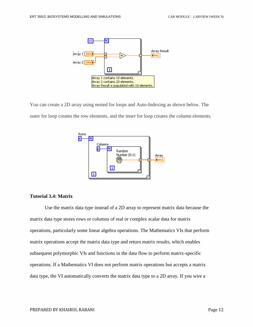
Be aware that if you enable Auto-Indexing on more than one loop tunnel and wire the for
loop count terminal, the number of iterations is equal to the smaller of the choices. For
example, in the figure below, the for loop count terminal is set to run 15 iterations, Array 1
contains 10 elements, and Array 2 contains 20 elements. If you run the VI in the figure
below, the for loop executes 10 times and Array Result contains 10 elements. Try this and
see it for yourself.
ERT 355/2: BIOSYSTEMS MODELLING AND SIMULATIONS LAB MODULE – LABVIEW (WEEK 9)
PREPARED BY KHAIRUL RABANI Page 12
You can create a 2D array using nested for loops and Auto-Indexing as shown below. The
outer for loop creates the row elements, and the inner for loop creates the column elements.
Tutorial 3.4: Matrix
Use the matrix data type instead of a 2D array to represent matrix data because the
matrix data type stores rows or columns of real or complex scalar data for matrix
operations, particularly some linear algebra operations. The Mathematics VIs that perform
matrix operations accept the matrix data type and return matrix results, which enables
subsequent polymorphic VIs and functions in the data flow to perform matrix-specific
operations. If a Mathematics VI does not perform matrix operations but accepts a matrix
data type, the VI automatically converts the matrix data type to a 2D array. If you wire a

ERT 355/2: BIOSYSTEMS MODELLING AND SIMULATIONS LAB MODULE – LABVIEW (WEEK 9)
PREPARED BY KHAIRUL RABANI Page 13
2D array to a VI that performs matrix operations by default, the VI automatically converts
the 2D array to a real or complex matrix, depending on the data type of the 2D array.
1. Create a new VI. Navigate to File»New VI.
2. On the Functions palette, navigate to Modern»Array,Matrix&Cluster and drag
the RealMatrix onto front panel.
3. Fill each element in the matrix of numeric indicators as shown below and rename
as Matrix A.

ERT 355/2: BIOSYSTEMS MODELLING AND SIMULATIONS LAB MODULE – LABVIEW (WEEK 9)
PREPARED BY KHAIRUL RABANI Page 14
4. Create a second matrix by repeat step 2 and 3. Fill each element of the matrix and
rename as Matrix B as shown below.
5. Wire the Matrix A and B to the x and y terminals of the add function.
6. Create indicator at output terminal of the add function.
7. Go to the front panel and run the VI.

ERT 355/2: BIOSYSTEMS MODELLING AND SIMULATIONS LAB MODULE – LABVIEW (WEEK 9)
PREPARED BY KHAIRUL RABANI Page 15
EXERCISE 1
1. Repeat Tutorial 3.4 by subtracts, multiply and divides the matrixes by using single
case selection VI.
2. Solving systems of linear equations is one of the most common computations in
science and engineering, and is easily handled by LabVIEW. Consider the following
set of linear equations. 5x = 3y − 2z + 10 8y + 4z = 3x + 20 2x + 4y − 9z = 9. This set
of equations can be re-arranged so that all the unknown quantities are on the left-
hand side and the known quantities are on the right-hand side.
5x − 3y + 2z = 10
−3x + 8y + 4z = 20
2x + 4y − 9z = 9

ERT 355/2: BIOSYSTEMS MODELLING AND SIMULATIONS LAB MODULE – LABVIEW (WEEK 9)
PREPARED BY KHAIRUL RABANI Page 16
Chapter 4: Formula Nodes
A Formula Node is a box where you enter algebraic formulas directly into the
Block Diagram. The Formula Node in the LabVIEW software is a convenient, text-based
node you can use to perform complicated mathematical operations on a block diagram
using the C++ syntax structure. It is most useful for equations that have many variables or
are otherwise complicated. The text-based code simplifies the block diagram and increases
its readability. Furthermore, you can copy and paste existing code directly into the Formula
Node rather than recreating it graphically.
In addition to text-based equation expressions, the Formula Node can accept text-
based versions of if statements, while loops, for loops, and do loops, which are familiar to
C programmers. These programming elements are similar but not identical to those you
find in C programming.
The MathScript Node implements similar functions but with the additional
functionality of a full .m file compiler, making it useful as a textual language for signal
processing, analysis, and math. LabVIEW MathScript is generally compatible with .m file
script syntax, which is widely used by alternative technical computing software. For
LabVIEW 2009 and later, the LabVIEW MathScript features are released separately in the
LabVIEW MathScript RT Module.

ERT 355/2: BIOSYSTEMS MODELLING AND SIMULATIONS LAB MODULE – LABVIEW (WEEK 9)
PREPARED BY KHAIRUL RABANI Page 17
It is useful when an equation is complicated or has many variables. Below is an example of
how you would implement y = x^2 + x + 1 with regular block diagram nodes:
It is much easier to use the Formula Node. Below is an example:
Tutorial 4.1: Using the Formula Node
Complete the following steps to create a VI that computes different formulas depending on
whether the product of the inputs is positive or negative.
1. Selecting File»New VI to open a blank VI.
2. Place a Formula Node on the block diagram.
1. Right-click on the diagram and navigate to Programming»Structures»Formula
Node.
2. Click and drag the cursor to place the Formula Node on the block diagram.

ERT 355/2: BIOSYSTEMS MODELLING AND SIMULATIONS LAB MODULE – LABVIEW (WEEK 9)
PREPARED BY KHAIRUL RABANI Page 18
3. Right-click the border of the Formula Node and select Add Input from the shortcut
menu.
4. Label the input variable x.
5. Repeat steps 3 and 4 to add another input and label it y.
6. Right-click the border of the Formula Node and select Add Output from the shortcut
menu.
ERT 355/2: BIOSYSTEMS MODELLING AND SIMULATIONS LAB MODULE – LABVIEW (WEEK 9)
PREPARED BY KHAIRUL RABANI Page 19
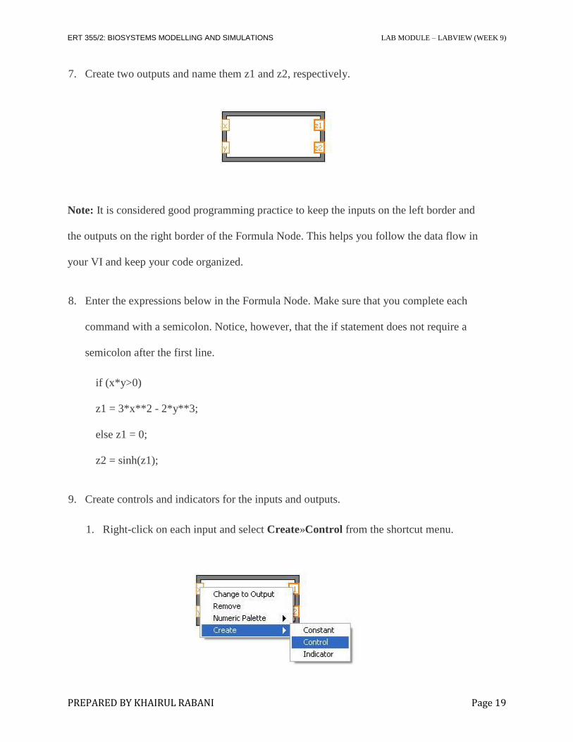
7. Create two outputs and name them z1 and z2, respectively.
Note: It is considered good programming practice to keep the inputs on the left border and
the outputs on the right border of the Formula Node. This helps you follow the data flow in
your VI and keep your code organized.
8. Enter the expressions below in the Formula Node. Make sure that you complete each
command with a semicolon. Notice, however, that the if statement does not require a
semicolon after the first line.
if (x*y>0)
z1 = 3*x**2 - 2*y**3;
else z1 = 0;
z2 = sinh(z1);
9. Create controls and indicators for the inputs and outputs.
1. Right-click on each input and select Create»Control from the shortcut menu.

ERT 355/2: BIOSYSTEMS MODELLING AND SIMULATIONS LAB MODULE – LABVIEW (WEEK 9)
PREPARED BY KHAIRUL RABANI Page 20
2. Right-click on each output and select Create»Indicator from the shortcut menu.
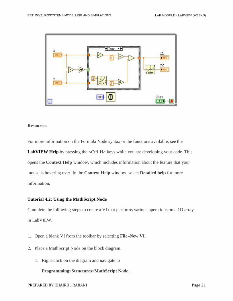
10. Place a While Loop with a stop button around the Formula Node and the controls. Be
sure to include a Wait (ms) function inside the loop to conserve memory usage. Your
block diagram should appear as follows.
11. Click the Run button to run the VI. Change the values of the input controls to see how
the outputs change.
In this case, the Formula Node helps minimize the space required on the block diagram.
Accomplishing the same task without the use of a Formula Node requires the following
code.
ERT 355/2: BIOSYSTEMS MODELLING AND SIMULATIONS LAB MODULE – LABVIEW (WEEK 9)
PREPARED BY KHAIRUL RABANI Page 21
Resources
For more information on the Formula Node syntax or the functions available, see the
LabVIEW Help by pressing the <Ctrl-H> keys while you are developing your code. This
opens the Context Help window, which includes information about the feature that your
mouse is hovering over. In the Context Help window, select Detailed help for more
information.
Tutorial 4.2: Using the MathScript Node
Complete the following steps to create a VI that performs various operations on a 1D array
in LabVIEW.
1. Open a blank VI from the toolbar by selecting File»New VI.
2. Place a MathScript Node on the block diagram.
1. Right-click on the diagram and navigate to
Programming»Structures»MathScript Node.

ERT 355/2: BIOSYSTEMS MODELLING AND SIMULATIONS LAB MODULE – LABVIEW (WEEK 9)
PREPARED BY KHAIRUL RABANI Page 22
2. Click and drag the cursor to place the MathScript Node on the block diagram.
3. In the same manner as you implemented in the Formula Node exercise, right-click on
the border and select Add Input from the shortcut menu. Label the input x.
4. Right-click the border and select Add Output from the shortcut menu. Repeat this
process to create three outputs labeled y, y1, and d. For LabVIEW 2010 and later select
Add Output»Undetected Variable.
5. Place an array of numeric controls on the front panel. Label the array x and wire it to
the x input of the MathScript Node on the block diagram.
6. In the MathScript Node, enter the following expressions:
y = x.^2;
y1 = y(1);
d = dot(x,y);
7. Create indicators for each of the three outputs by right-clicking each output and
selecting Create»Indicator from the shortcut menu.
8. Place a While Loop with a stop button around the MathScript Node and the controls.
Be sure to include a Wait (ms) function inside the loop to conserve memory usage.
Your block diagram should appear as follows.

ERT 355/2: BIOSYSTEMS MODELLING AND SIMULATIONS LAB MODULE – LABVIEW (WEEK 9)
PREPARED BY KHAIRUL RABANI Page 23
9. On the front panel, expand the arrays to show multiple elements. With the cursor, grab
the bottom middle selector of the array and drag it down to show multiple elements.
10. Begin by placing a 1, 2, and 3 in the first three elements of the x control. Your front
panel should look similar to the one below. Note that the fourth and fifth elements are
grayed out. This is because they are not initialized. You can initialize them by clicking
inside the cell and entering a value. To uninitialize a cell, right-click the element and
select Data Operations»Delete Element from the shortcut menu.

ERT 355/2: BIOSYSTEMS MODELLING AND SIMULATIONS LAB MODULE – LABVIEW (WEEK 9)
PREPARED BY KHAIRUL RABANI Page 24
11. Click the Run button. Change the values of the elements in the array to see how the
outputs change.