labour market attractiveness in the...

S TAT I S C T I C A LW O R K I N G P A P E R S

S TAT I S T I C A LW O R K I N G P A P E R S

Labour market attractiveness in the EU

2018 edition


JOAO SOLLARI LOPES, SONIA QUARESMA AND MARCO MOURA 2018 edition

Labour market attractiveness in the EU 2018 edition

Manuscript completed in January 2018

Neither the European Commission nor any person acting on behalf of the Commission is responsible for

the use that might be made of the following information.

Luxembourg: Publications Office of the European Union, 2018

© European Union, 2018

Reuse is authorised provided the source is acknowledged.

The reuse policy of European Commission documents is regulated by Decision 2011/833/EU (OJ L 330,

14.12.2011, p. 39).

Copyright for photographs: © Shutterstock/Artens

For any use or reproduction of photos or other material that is not under the EU copyright, permission

must be sought directly from the copyright holders.

For more information, please consult: http://ec.europa.eu/eurostat/about/policies/copyright

The information and views set out in this publication are those of the authors and do not necessarily

reflect the official opinion of the European Union. Neither the European Union institutions and bodies nor

any person acting on their behalf may be held responsible for the use which may be made of the

information contained therein.

ISBN 978-92-79-80731-2 ISSN 2315-0807 doi: 10.2785/252238 KS-TC-18-002-EN-N

http://ec.europa.eu/eurostat/about/policies/copyright

Abstract

3 Labour market attractiveness in the EU

Abstract In this work we present a data product developed for the European Big Data Hackathon, a

competition between 22 teams which took place in March 2017. This data product is divided in two

parts: an exploration part, which is aimed to better understand the EU global labour market and to

capture its heterogeneity; and an inferential part, whose goal is to establish associations between

characteristics of the EU labour market and indicators designed to capture important aspects of the

labour market (i.e. Skills mismatch, Mobility and Emigration). For the exploration part, we developed

the concept of Labour Market Attractiveness, which consists of a combination of variables from 6

Eurostats datasets on different subjects (i.e. demographics; earnings structure; education and

training; life conditions; employment and unemployment; and national accounts). Using data mining

techniques, such as social networks and clustering analysis, we showed that this combined set

consistently captured the country-level heterogeneity in the EU, forming well-defined clusters. For the

inferential part, we used model selection analysis and weighted network correlation analyses to

establish associations between the characteristics of the EU labour market and the labour market

indicators. Using model selection, we showed that the Labour Market Attractiveness set was able to

capture well the variations of these indicators across EU. We further showed that the Labour Market

Attractiveness set can be summarized by 6 Eigenvariables (i.e. ‘Unemployment’, ‘Poverty’, ‘Ageing

Population’, ‘Education (Employed Adults)’, ‘Employment’ and ‘Earnings structure’), whose

association with labour market indicators was also assessed. We argue that the combination of both

exploration and inferential parts can shed some light on the complex dynamics of the EU labour

market. In fact, the final goal of our developed product is to help setting effective policies to tackle

typical problems of a fast-changing global labour market environment.

Key-words: Labour Market Attractiveness, Labour Market Mobility, Emigration, Skills Demand, Skills

Supply.

Acknowledgements:

This work has been carried out by Joao Sollari Lopes*, Sonia Quaresma† and Marco Moura‡ for the

‘European Big Data Hackathon 2017’ competition and the follow-up meeting ‘From Prototype to

Production’ organized by Eurostat Task Force ‘Big Data’ and Cedefop.

* [email protected]

† [email protected]

‡ [email protected]

mailto:[email protected]



Contents


Contents 1. Introduction and context ................................................................................................... 5

2. Material and methods ........................................................................................................ 6

2.1. Databases ....................................................................................................................... 6

2.2. Variables considered ...................................................................................................... 6

2.3. Methods .......................................................................................................................... 7

3. Results ................................................................................................................................ 9

4. Discussion and conclusions ........................................................................................... 14

List of acronyms ......................................................................................................................... 16

References................................................................................................................................... 17

ANNEX 1 ...................................................................................................................................... 18

Eurostat datasets for Labour Market Attractiveness set .......................................................... 18

ANNEX 2 ...................................................................................................................................... 19

Eurostat datasets for labour market indicators ........................................................................ 19

ANNEX 3 ...................................................................................................................................... 20

Summary statistics on Labour Market Attractiveness set ........................................................ 20

ANNEX 4 ...................................................................................................................................... 22

Summary statistics on labour market indicators ...................................................................... 22

ANNEX 5 ...................................................................................................................................... 23

Averages of top 10 separator variables of clusters ................................................................. 23

ANNEX 6 ...................................................................................................................................... 24

Correlation between labour market indicators and Labour Market Attractiveness .................. 24

ANNEX 7 ...................................................................................................................................... 26

1 Introduction and context


1. Introduction and context The European Big Data Hackathon took place in March 2017 — in parallel with the conference New

Techniques and Technologies for Statistics. This event was organised by Eurostat and gathered 22

teams from 21 European countries. The aim was to compete for the best data product combining

official statistics and Big Data to support policy makers in a pressing policy question, namely, ‘How to

tackle the mismatch between jobs and skills at regional level in Europe?’. Indeed, the mismatch

between the available skills of the labour force and the skills required by the labour market entail

significant economic and social costs for individuals and firms. Furthermore, a strong education and

an efficient development of skills are essential for thriving in the emerging new economy and fast-

changing labour market (1). Nonetheless, a survey from 2014 showed that skills mismatch (i.e. over-

qualification, under-qualification) remains at 45% in the European Union (EU) (CEDEFOP, 2015).

This led to the publication of the EU Guidelines for the employment policies of the Member States in

2015, which called for enhancing labour supply, skills and competences (2).

Our data product entailed two parts: an exploration part, in which we aimed to better understand the

EU global labour market and to capture its heterogeneity; and a inferential part, where we

established associations between characteristics of the EU labour market and indicators designed to

capture important aspects of the labour market, such as Mobility, Emigration and the previously

mentioned Skills mismatch.

For the first exploration part, we developed the concept of Labour Market Attractiveness. This

concept has to be taken carefully and our approach should be seen as a first-step towards a more

mature definition. We considered 17 variables from 6 Eurostat datasets with information on

demography, earnings structure, education and training, life conditions, employment and

unemployment, and national accounts (3). These variables were broken by several categorical levels

(e.g. ‘age groups’, ‘level of education’, ‘qualifications’, ‘occupations’) originating more than 70

variables. Data mining techniques were then considered to analyse the compiled Labour Market

Attractiveness set: distances between regions were calculated and visualized using networks; the

regions were clustered using these distance; and the clusters were characterized using over-

representation analysis.

For the second inferential part, we considered the characteristics of the EU labour market extracted

from the first exploration part and studied their association with specific indicators designed to

capture different aspects of the labour market. These indicators were developed using Eurostat

datasets and comprised of Skills mismatch, Mobility and Emigration at country-level. The levels of

association were studied using model selection on multivariate linear regression analyses. We

further constructed Eigenvariables from the considered Labour Market Attractiveness set and

performed weighted correlation network analysis on the labour market indicators.

We argue that the combination of the exploration and association studies can be invaluable to fully

understand the influences on the complex dynamics of the EU labour market. Indeed, the final goal is

to use this understanding to help setting policies to tackle such problems as localized excess or

deficit of available labour force and/or of specific labour skills, typical problems of the fast-changing

EU labour market.

(1) https://ec.europa.eu/commission/publications/skills-education-and-lifelong-learning-european-pillar-social-rights_en

(2) Council Decision (EU) 2015/1848 of 5 October 2015

(3) http://ec.europa.eu/eurostat/data/database

https://ec.europa.eu/commission/publications/skills-education-and-lifelong-learning-european-pillar-social-rights_en

http://ec.europa.eu/eurostat/data/database

2 Material and methods


2. Material and methods

2.1. Databases

For the construction of the Labour Market Attractiveness set, we considered 6 Eurostat datasets to

capture different aspects of the attractiveness of a labour market. Thus, we chose reg_demo for

Demographics data, earn for Earnings structure data, edtr for data on Education and training, ilc for

Life conditions information, employ for Employment and unemployment data, and na10 for National

accounts data. These main datasets comprised of 17 smaller datasets described in Annex 1. Except

for two datasets, all of them refer to the year 2014. The exceptions were educ_uoe_fine06 (i.e. Total

public expenditure on education) and nama_10r_2hhinc (i.e. Income of households), which referred

to 2013 in order to obtain a more complete dataset.

For the construction of the Labour Market indicators in study, we also considered several Eurostat

datasets (see Annex 2). To study Mobility and Emigration, we used the datasets lfso_14leeow on

Labour Force and migr_emi2 on Emigration, respectively. For the construction of the Skills mismatch

indicator, we assumed two major simplifications, however, these simplifications do not affect our

product in terms of proof-of-concept and can be dropped in later developments. The first one was to

use previously cleaned and treated data on job vacancies and education attainment from the

Eurostat’s labour and edtr datasets, respectively. Instead, a better approach would be to use freshly

collected job portals data, but the use of this data would have two caveats: a) the cleaning and

structuring of the data would require a considerable expertise on the subject; b) the normalizing of

the data, using for example marginal calibration techniques, would require detailed demographic

data and, more importantly, well-defined populations. The second simplification was to use an ad hoc

mapping between qualifications (classified using ISCED-F 13) and the cross between occupations

(defined using ISCO-08) and economic activity (defined using NACE Rev. 2). Nevertheless, a formal

mapping system is scheduled to be released soon by European Skills, Qualifications and

Occupations (ESCO) from the European Commission.

2.2. Variables considered

For each of the 17 Eurostat datasets composing Labour Market Attractiveness set, we extracted one

variable. These 17 main variables were broken by several categorical levels [i.e. type of contract,

age groups, level of education (ISCED 11), economic activity (NACE Rev. 2) and occupation title

(ISCO-08), see Annex 7 for a full description] originating 76 variables. The entire set of these

variables compose the Labour Market Attractiveness set (Table 1 and Annex 3).

Table 1: Variables of Labour Market Attractiveness

variable description dataset units

ARPR At-risk-of-poverty rate ilc_li41 PC_POP

AROPE At-risk-of-poverty or social exclusion ilc_peps11 PC_POP

earn_OC[...]_Nace[...] Earning by ISCO-08 and NACE Rev. 2 earn_ses_hourly MN_PPS

emp_T[...] Employment by work contract lfst_r_lfe2eftpt PC_POP_YGE15

emp_Y[...] Employment by age lfst_r_lfe2emp PC_POP_Y[...]

emp_Y[...]_ED[...] Employment by age and ISCED 11 lfst_r_lfe2eedu PC_EMP_Y[…]

emp_Y[...]_Nace[...] Employment by age and NACE Rev. 2 lfst_r_lfe2en2 PC_EMP_Y[...]

expend_ED5-8 Public expenditure on education educ_uoe_fine06 PC_GDP

disp_income Disposable income nama_10r_2hhinc PPCS_HAB

GDP Gross Domestic Product nama_10r_2gdp PPS_HAB

GVAgr Gross Value Added growth nama_10r_2gvagr PCH_PRE

low_work Very low work intensity ilc_lvhl21 PC_POP_YLE60



mat_depriv Severe material deprivation ilc_mddd21 PC_POP

pop_Total Population demo_r_d2jan NR

pop_Y[…] Population by age demo_r_d2jan PC_POP

rooms_pp Number of rooms per person ilc_lvho04n AVG

training Participation in education and training trng_lfse_0 PC_POP_Y25–64

unemp_Y[...] Unemployment by age lfst_r_lfu3pers PC_POP_Y[…] PC_POP, Percentage of Population; MN_PPS, Mean by group in Purchasing Power Standard; PC_POP_YGE15, Percentage of

Population greater or equal than 15 years old; PC_POP_Y[...], Percentage of Population of given age group; PC_GDP, Percentage of Gross Domestic Product; PPCS_HAB, Purchasing Power Consumption Standard per inhabitant; PPS_HAB, Purchasing Power Standard per inhabitant; PCH_PRE, Percentage change on previous period; PC_POP_YLE60, Percentage of Population less or equal than 60 years old; NR, Number; AVG, Average; PC_Y25–64, Percentage of Population between 25 and 64 years old.

The Mobility indicator, or Labour market mobility, was calculated as the percentage of foreigner

employees, and should reflect the attractiveness of a Labour Market to foreigners. The Emigration

indicator was calculated as the percentage of emigrants in a country, and should reflect the

willingness of the population to leave the country. The Skills mismatch was calculated as the

Euclidean difference between the proportion of students and the proportion of job vacancies by field

of education (classified using ISCED-F 13, see Annex 7). Since job vacancy information is available

only by occupations (defined using ISCO-08) and economic activity (defined using NACE Rev. 2),

there was the need to map fields of education to the cross between occupations and economic

activities using the previously mentioned ad hoc mapping system. Table 2 summarizes the variables

used as Labour Market indicators. Note that, due to missing data Skills mismatch had only

information on 8 countries (Annex 4).

Table 2: Labour market indicators

variable description dataset units

Skills mismatch Mismatch between Jobs and Skills educ_uoe_grad02, jvs_a_nace2 DIST

Mobility Labour Market mobility lfso_14leeow PC_EMP

Emigration Emigration rate migr_emi2 PC_POP DIST, Euclidean distance between Jobs and Skills; PC_EMP, Percentage of employed Population; PC_POP, Percentage of Population.

2.3. Methods

Several data mining techniques were considered to analyse the compiled Labour Market

Attractiveness set and the labour market indicators: Social network analysis (SNA); Partition-around-

medoids (PAM) (Reynolds et al.,1992); Over-representation analysis (ORA); Model selection using

multivariate linear regression analysis (Calcagno and Mazancourt, 2010); and Weighted correlation

network analysis (WCNA) (Langfelder and Horvath, 2008).

A social network was used to visualize the entire Labour Market Attractiveness set according to the

similarities between the countries. These similarity values were calculated as the additive inverse of

weighted Euclidean distances between countries. The distances were calculated using all the 76

variables weighted in such a way that each set of variables originated from one of the 17 main

variables had a weight of one. This weighting scheme was employed to insure that there was no bias

towards main variables broken in many secondary variables. Prior to the calculation of the distances,

the variables were made dimensionless using a min-max transformation (4). Finally, the network was

constructed on the similarities above 0.65 using the ‘Fruchterman–Reingold’ algorithm as

implemented in the R package ‘sna’ (Butts, 2016).

The countries were clustered using a PAM analysis on the previously calculated weighted Euclidean

distances. This analysis uses silhouette widths to partition data into clusters. Silhouette widths are

calculated by comparing how close one element is to the remaining elements of its cluster with how

close it is to the elements of the nearest neighbour cluster. A clustering analysis can then be



characterized by calculating the average silhouette width of all the elements. The number of

considered clusters k was chosen by running the analysis with all possible number of clusters (k = 2,

3, ..., n – 1, where n was the number of subjects) and examining their average silhouette width. The

PAM analysis was implemented in the R package ‘cluster’ (Maechler et al., 2016).

In order to describe the clusters created, we performed an ORA on each variable of the Labour

Market Attractiveness set. This analysis can identify which variables are over-represented in each

created cluster. Before performing this analysis the variables were discretized by defining a cut-off on

the 90th percentile (over-representation of the higher values) and on the 10th percentile (over-

representation of the lower values). The significance of these analyses was set to p-value = 0.05 (5).

In order to study the relation between the Labour Market indicators and the variables of the Labour

Market Attractiveness set, we fitted multivariate linear regressions using the indicators as response

variables. Using heuristics from the R package ‘glmulti’ (Calcagno, 2013), we defined which model

best predicted each indicator. The model selection was performed using an exhaustive screening

when the number of models was less than 200 000 or using a genetic algorithm approach as

implemented in the used R package. To assure a good coverage when running the genetic algorithm

approach, two replicas were run with two sets of parameters each (1st set: popsize = 100, mutrate =

0.001, sexrate = 0.1, imm = 0.3, deltaM = 0.05, deltaB = 0.05, conseq = 5; 2nd set: popsize = 200,

mutrate = 0.01, sexrate = 0.2, imm = 0.6, deltaM = 0.005, deltaB = 0.005, conseq = 10). The 100

models with the lowest AICc were stored. The maximum number of predictors for the models was

chosen to be the hard threshold [i.e. maximum predictors is m such that m = n – 1 – 3, where n is the

number of subjects]. Before performing model-choice, the dataset was pre-processed by removing

variables until obtaining a set of 30 using the following steps: 1) any variable with missing data; 2)

variables highly correlated among them (ρ < 0.90); 3) variables little correlated with the response

variable. This analysis allowed us to take a multivariate approach to establish associations; however,

it had two caveats: firstly we had to discard all the variables with missing data; secondly looking at a

best model may overshadow other interesting models.

To study the Labour Market indicators on a reduced number of variables, WCNA was employed to

extract Eigenvariables from the Labour Market Attractiveness set using the R package ‘WGCNA’

(Langfelder and Horvath, 2008). Eigenvariables (or Modules) are groups of variables constructed

based on pairwise distances. The distances are obtained by calculating Topological Overlap

Matrices using the absolute value of Spearman correlations raised to the k power. The value of k

was chosen by taking the minimum value above 90% of the best scored value, where the scores

were calculated as suggested by the authors of the package (Langfelder and Horvath, 2008). The

groups of variables were then created using weighted networks with the following settings: minimum

module size = 2, cluster splitting level = 4, dynamic tree cut method = ‘hybrid’, and merge cut-off

height = 0.2. Eigenvariables are calculated as the first Principal Component of each grouping of

variables. The Module membership of a variable can be calculated as the correlation to its belonging

Eigenvariable. Similarly, the quality of a Module can be assessed by calculating the average of the

Module membership of all its variables. Finally, the association between the constructed

Eigenvariables and the labour market indicators can be calculated using Spearman correlations (-

0.30 < ρ < 0.30). Before performing WCNA, the dataset was pre-processed by removing variables

with more than 15% of missing data.

All the analysis (including the ad hoc mapping system for constructing the Skills mismatch indicator)

can be reproduced using R scripts stored in a github repository (6).

(4) min-max transformation: zi = (xi – min(x))/(max(x) – min(x)), where z is the transformed variable that ranges from 0 to 1.

(5) H0 = elements of a cluster are equally likely to be over or under the 90

th (or 10

th) percentile of the distribution of a variable.

(6) https://github.com/jsollari/EUhackathon2017.

https://github.com/jsollari/EUhackathon2017

3 Results


3. Results Our first approach was to visualize the entire Labour Market Attractiveness set by constructing a

social network based on distances between countries (Figure 1). From this analysis we saw a clear

separation between Northern and Western European countries and Eastern European countries,

while Southern European countries seemed to somewhat make the bridge between these two main

blocks. More in detail, we observed a group formed by Denmark (DK), Finland (FI), Sweden (SE),

Netherlands (NL) and Austria (AT), and another by France (FR), Germany (DE) and the United

Kingdom (UK). On the other hand, Czech Republic (CZ), Estonia (EE), Lithuania (LT), Poland (PL),

Slovenia (SI) and Slovakia (SK) seemed to form a group, while Bulgaria (BG), Hungary (HU), Latvia

(LV) and Romania (RO) seemed to form another one. Belgium (BE), Malta (MT) and Portugal (PT)

were positioned in the centre of the network. We also observed strong links between pairs of

countries, i.e. Greece (EL) and Croatia (HR), Italy (IT) and Spain (ES), and Cyprus (CY) and Malta.

Finally, both Luxemburg (LU) and Ireland (IE) seemed to be far apart from all the other countries.

Figure 1: Country social network using Labour Market Attractiveness set

Following the construction of a country network, we performed a clustering analysis on the data

(Figure 2). This analysis gave a more detailed overview of the grouping with very consistent clusters

(separation values always above 2, Table 3). The Northern and Western European countries were

further divided in Cluster 4 (DE, UK, FR) and Cluster 5 (DK, SE, FI, NL), while the Eastern European

countries were divided in Cluster 2 (BG, RO, LV, HU) and Cluster 3 (CZ, SK, SI). As in the previous

analysis, some countries were paired, such as in Cluster 7 (EL, HR) and in Cluster 8 (ES, IT), while

LU and IE remained separated in Clusters 9 and 10, respectively. Interestingly, we observed two

3 Results


considerably heterogeneous groupings Cluster 1 (MT, CY, BE, AT) and Cluster 6 (EE, LT, PT, PL).

Overall, the SNA and the PAM analysis gave very consistent results.

Figure 2: Cluster analysis using Labour Market Attractiveness set. Average silhouette

width for all possible number of clusters (left). Silhouette width of regions considered

for 10 clusters (right)

Table 3: Description of clusters

cluster NUTS(a) n sep

AT-BE-CY-MT MT, CY, BE, AT 4 2.66

BG-HU-LV-RO BG, RO, LV, HU 4 2.49

CZ-SK-SI CZ, SK, SI 3 2.31

DE-FR-UK DE, UK, FR 3 3.19

DK-FI-NL-SE DK, SE, FI, NL 4 2.66

EE-LT-PL-PT EE, LT, PT, PL 4 2.31

EL-HR EL, HR 2 3.53

ES-IT ES, IT 2 3.10

IE IE 1 3.75

LU LU 1 4.68 (a) Order of countries reflects belongingness to cluster (i.e. silhouette width).

n, number of elements of the cluster; sep, separation of the cluster (i.e. minimal dissimilarity between an observation of the cluster and an observation of another cluster).

In order to obtain a general characterization of the clusters, we looked at variables that provided a

higher separation between the groupings, namely: Gross Domestic Product (GDP), public

expenditure in higher education, total population size, disposable income and proportion of adults

working in Financial and insurance activities (see Annex 5). For a characterization of each specific

3 Results


cluster, we further performed an ORA on discretized variables (Table 4). Thus, we found that Cluster

1 (AT, BE, CY, MT) was characterized as having small-sized populations, high proportions of

youngsters and high proportions of employed youngsters with higher education. Cluster 2 (BG, HU,

LV, RO) was mostly characterized as having high rates of poverty, low disposable incomes and low

expenditures in higher-education. Cluster 3 (CZ, SK, SI) was characterized as having high

proportions of adults in the population, of which the employed ones had high proportions achieving

secondary education and low proportions achieving only primary education. Cluster 4 (DE, FR, UK)

was characterized as having large-sized populations with high proportions of children and high

disposable incomes. Cluster 5 (DK, FI, NL, SE) was characterized as having high rates of employed

youngsters and adults, high expenditures in higher education and low rates of poverty. Cluster 6 (EE,

LT, PL, PT) was characterized as having high proportions of employed elders. Cluster 7 (EL, HR)

was characterized as having high unemployment rates of youngsters and low employment rates of

adults. Finally, Cluster 8 (ES, IT) was characterized as having both low proportions of youngsters in

the population and of employed youngsters. Regarding the single-element Clusters 9 and 10, we

were unable to perform ORA since obtaining significant statistics in these cases is considerably

difficult. Nonetheless, we note that IE (Cluster 9) had the highest proportion of children and the

highest Gross Value Added growth (GVAgr) of the whole EU-28 countries, while LU (Cluster 10) had

the highest proportion of employed adults with higher education and the highest GDP.

Table 4: Characterization of clusters

cluster Over-represented variables

AT-BE-CY-MT > P90: emp_Y[15–24]_ED[5–8]; emp_Y[15–24]_Nace[F]; pop_Y[15–24]; rooms_pp.

< P10: pop_Total.

BG-HU-LV-RO > P90: AROPE; emp_Y[15–24]_Nace[J]; mat_depriv.

< P10: disp_income; earn_OC[1–9]_Nace[B–F]; earn_OC[2–5, 7–9]_Nace[G-N];

earn_OC[1–9]_Nace[P–S]; emp_Y[15–24, 25–64]_Nace[O–Q]; expend_ED[5–8]; GDP;

training.

CZ-SK-SI

> P90: emp_Y[15–24, 25–64]_ED[3–4]; emp_Y[15–24]_Nace[B–E]; emp_Y[25–

64]_Nace[B-E, F]; pop_Y[25–64].

< P10: emp_Y[25–64]_ED[0–2].

DE-FR-UK > P90: disp_income; pop_Total; pop_Y[0–14].

< P10: emp_Y[15–24]_Nace[A].

DK-FI-NL-SE

> P90: earn_OC[7–9]_Nace[B–F]; earn_OC[5, 9]_Nace[G–N]; earn_OC[6, 8]_Nace[P–

S]; emp_Y[15–24, 25–64]; emp_Y[15–24]_ED[0–2]; emp_Y[15–24]_Nace[M–N];

emp_Y[25–64]_Nace[J, M–N, O–Q]; expend_ED[5–8]; pop_Y[65–74]; training.

< P10: ARPR; AROPE; emp_Y[15–24]_ED[3–4, 5–8]; emp_Y[25–64]_Nace[G–I];

mat_depriv; pop_Y[25–64].

EE-LT-PL-PT > P90: emp_Y[GE65].

< P10: earn_OC[1]_Nace[G–N]; emp_Y[25–64]_Nace[J, K].

EL-HR > P90: unemp_Y[15–24].

< P10: emp_Y[25–64]; emp_Y[25–64]_Nace[L].

ES-IT > P90: none.

< P10: emp_Y[15–24]; pop_Y[15–24].

IE > P90: none.

< P10: none.

LU > P90: none.

< P10: none.

For the inferential part of the framework, we first calculated simple Spearman correlations between

each variable of the Labour Market Attractiveness set and the labour market indicators (Annex 6).

We noted that while Skills mismatch was only significantly associated (p-value < 0.05) to ‘emp_Y[15–

24]’ (Proportion of employed youth), Mobility was associated to more than 40 variables and

Emigration to about 10 variables. Therefore, our next approach was to perform a model selection

3 Results


using multivariate linear regression models to find which group of variables from the Labour Market

Attractiveness set could explain better the labour market indicators. We observed that Skills

Mismatch across EU-28 could be well explained using ‘emp_Y[15–24]’ and ‘emp_Y[15–24]_Nace[M–

N]’ (Proportion of employed youth in Professional, scientific and technical activities; administrative

and support service activities) with a R2 = 0.94 (Table 5). Mobility was best modelled considering

‘emp_Y[25–64]_Nace[L]’ (Proportion of employed adults in Real estate activities), ‘emp_Y[25–

64]_Nace[K]’ (Proportion of employed adults in Financial and insurance activities) and ‘emp_Y[15–

24]_Nace[B–E]’ (Proportion of employed youths in Industry) achieving a R2 = 0.79 (Table 6).

Regarding Emigration the variables of the best model were ‘emp_Y[25–64]_Nace[K]’ (Proportion of

employed adults in Financial and insurance activities), ‘emp_Y[15–24]_ED[5–8]’ (Proportion of

employed youths with Tertiary Education), ‘emp_Y[15–24]_Nace[O–Q]’ (Proportion of employed

youths in Public administration, defence, education, human health and social work activities),

‘pop_Total’ (Total population size) and ‘emp_Y[15–24]_Nace[B–E]’ (Proportion of employed youth in

Industry) with a R2 = 0.83 (Table 7).

Table 5: Summary Table for best multivariate model for Skills Mismatch

Variables Estimate Std. Error t-value Pr(>|t-value|)

(Intercept) 100.60 8.694 11.570 <0.001

emp_Y15–24 -3.18 0.356 -8.920 <0.001

emp_Y15–24_NaceM-N 6.56 1.000 6.560 0.001

skills_mismatch ~ emp_Y15–24 + emp_Y15–25_NaceM–N

RSS = 5.51 (5 d.f.) R

2 = 0.94, R

2-adjusted = 0.92

F(2,5) = 43.76 (p-value < 0.001) Note: 20 data entries and 34 variables were removed to keep only complete-cases; 10 variables highly correlated among them (ρ > 0.90)

and 2 variables least correlated with dependent variable (ρ < 0. 06) were removed to run analysis at the most with 30 variables.

Table 6: Summary Table for best multivariate model for Mobility


(Intercept) 1.82 6.196 0.290 0.772

emp_Y25–64_NaceK 4.61 0.711 6.470 <0.001

emp_Y25–64_NaceL 10.04 2.892 3.470 0.002

emp_Y15–24_NaceB–E -0.38 0.198 -1.930 0.067

mobility ~ emp_Y25–64_NaceK + emp_Y25–64_NaceL + emp_Y15–24_NaceB–E

RSS = 7.10 (21 d.f.) R

2 = 0.79, R

2-adjusted = 0.76

F(3,21) = 25.85 (p-value < 0.001) Note: 3 data entries and 34 variables were removed to keep only complete-cases; 1 variables highly correlated among them (ρ > 0.90)

and 11 variables least correlated with dependent variable (ρ < 0. 15) were removed to run analysis at the most with 30 variables.

Table 7: Summary Table for best multivariate model for Emigration


(Intercept) 0.52 0.276 1.900 0.071

emp_Y25–64_NaceK 0.18 0.031 5.790 <0.001

emp_Y15–24_ED5–8 0.03 0.006 4.420 <0.001

emp_Y15–24_NaceO–Q -0.03 0.011 -2.880 0.009

pop_Total 0.00 0.000 -2.500 0.020

emp_Y15–24_NaceB–E -0.01 0.008 -1.870 0.075

3 Results


emigration ~ emp_Y25–64_NaceK + emp_Y15–24_ED5–8 + emp_Y15–24_NaceO–Q + pop_Total + emp_Y15–24_NaceB–E RSS = 0.27 (22 d.f.) R

2 = 0.83, R

2-adjusted = 0.79

F(5,22) = 21.55 (p-value < 0.001) Note: 34 variables were removed to keep only complete-cases; 1 variable highly correlated among them (ρ > 0.90) and 11 variables least

correlated with dependent variable (ρ < 0. 11) were removed to run analysis at the most with 30 variables.

Our final approach for the inferential part was to use WCNA to study associations using a reduced

variable set. Indeed, we were able to reduce the Labour Market Attractiveness set to 6

Eigenvariables, namely, ‘Unemployment’, ‘Poverty’, ‘Ageing Population’, ‘Education (Employed

Adults)’, ‘Employment’ and ‘Earnings structure’ (Table 8). Considering these Eigenvariables (Table

9), we found that Skills Mismatch is very negatively associated to ‘Employment’ (ρ = -0.69, p-value =

0.058) and moderately negatively associated to ‘Education (Employed Adults)’ (ρ = -0.38, p-value =

0.352), while being moderately associated to ‘Poverty’ (ρ = 0.38, p-value = 0.352) and

‘Unemployment’ (ρ = 0.36, p-value = 0.385). Mobility is strongly associated to ‘Earnings structure’ (ρ

= 0.59, p-value = 0.002) and moderately associated to ‘Employment’ (ρ = 0.35, p-value = 0.082).

Lastly, Emigration is very negatively associated to ‘Education (Employed Adults)’ (ρ = -0.50, p-value

= 0.007) and moderately negatively associated to Ageing Population (ρ = -0.36, p-value = 0.063).

Table 8: Eigenvariables of Labour Market Attractiveness set

Eigenvariables n mean MM Variables (>0.75 MM)

Unemployment 3 0.83

+: emp_Y[15–24]_Nace[G–I]; unemp_Y[15–24,

GE25].

-: none.

Poverty 2 0.95 +: ARPR; AROPE.

-: none.

Ageing Population 2 0.86 +: pop_Y[GE75].

-: pop_Y[15–24].

Education (Employed Adults) 4 0.71 +: emp_Y[25–64]_ED[3–4].

-: emp_Y[25–64]_ED[0–2]

Employment 4 0.80 +: emp_Y[15–24, 25–64]

-: none.

Earnings 51 0.76

+: earn_OC[1–5, 7–9]_Nace[B–F]; earn_OC[1–5,

7–9]_Nace[G–N]; earn_OC[1–5, 9]_Nace[P–S];

emp_T[P]; emp_Y[25–64]_Nace[M_N, O–Q];

GDP; rooms_pp; training;

-: mat_depriv. n, number of variables grouped in Eigenvariable; MM, module membership calculated as the correlation to belonging Eigenvariable.

Note: 8 variables with more than 15% of missing data were removed. 2 variables did not group into any Eigenvariable.

Table 9: Correlation between labour market indicators and Eigenvariables

Eigenvariables Skills Mismatch Mobility Emigration

Unemployed 0.36 (0.385) - -

Poverty 0.38 (0.352) - -

Ageing Population - - -0.36 (0.063)

Education (Employed Adults) -0.38 (0.352) - -0.50 (0.007)

Employed -0.69 (0.058) 0.35 (0.082) -

Earnings - 0.59 (0.002) - (-) correlations between -0.30 and 0.30.

Note: Correlations calculated using Spearman correlation (p-values between brackets).

4 Discussion and conclusions


4. Discussion and conclusions The use of the Labour Market Attractiveness set aimed to capture the heterogeneity of the EU global

labour market. For this purpose, we chose a broad collection of socio-demographic and economic

information. The chosen set of variables seemed to successfully describe the EU space as the

country network built showed complex interactions between the regions. Indeed, there seems to be a

main separation between Northern and Western Europe and Eastern Europe, which at a finer detail

revealed a far more complex net of connections. Thus, we observed a strongly connected group of

Scandinavian countries (DK, FI and SE), a group of the most populous countries (FR, DE and UK),

two distinct groups of Eastern European countries (CZ, EE, LT, PL, SI and SK; and BG, HU, LV and

RO), several pairings (EL and HR; IT and ES; and CY and MT), and two single-element groups (LU;

and IE).

The social network approach was complemented using a clustering analysis coupled with ORA to

extract the clusters defining characteristics. These characteristics can reflect different degrees of

attractiveness depending on the stakeholder. Thus, Cluster 3 (CZ, SI and SK) can be more attractive

when looking for labour forces composed mostly by adults, while Cluster 1 (AT, BE, CY and MT) can

be attractive when looking for younger labour forces. Similarly, Cluster 2 (BG, LV, HU and RO) can

be attractive for enterprises looking for low-waged economies, while Cluster 5 (DK, SE, FI and NL)

and Cluster 4 (FR, DE and UK) can be attractive for job seekers looking for high-paid jobs.

Stakeholders interested in labour markets fairly open to elders can look at Cluster 6 (EE, LT, PL and

PT). Nevertheless, characteristics such as high poverty rates, high unemployment, low-level of

education and low public expenditure in education are generally unattractive.

The main goal for developing this exploration framework was to extract useful information from data

to help policy-makers define strategies to tackle labour market problems. In fact, we argue that the

characteristics extracted from the data can be invaluable to define strategies more suitable for each

particular regional case. For example, taking into account countries characteristics such as ageing

labour forces (Cluster 6: EE, LT, PL and PT), ageing population (Cluster 5: DK, FI, NL and SE; and

Cluster 8: ES and IT) or highly skilled labour forces (Cluster 1: AT, BE, CY and MT; and Cluster 10:

LU) can be of utmost importance when implementing policies to reduce Skills mismatch. Moreover,

knowing of high unemployment (Cluster 7: EL and HR) and low access to employment (Cluster 8: ES

and IT) can be important to diagnose potential labour market problems.

Using the inferential part of the framework, we aimed to establish associations between indicators

relevant to labour market (i.e. Skills mismatch, Mobility, Emigration) and the characteristics of the

labour market itself. Interestingly, we noticed that the clustering scheme did not reflect the

distribution of values of the indicators, thus, we considered the countries separately. Using

multivariate linear regressions, we found that all the indicators could be successfully modelled using

variables from the Labour Market Attractiveness set with R2 between 0.79 and 0.94. As mentioned

before, results from a model-selection analysis need to be looked at carefully, particularly, because

the best models often overshadow other interesting ones. Nevertheless, we noted that, albeit being

defined only by 8 points, Skills mismatch could be well captured by considering information on

employed youth. In particular, there seems to be an inverse relation between employed youth and

Skills mismatch. Regarding Mobility, we found that its variation can be explained well by employed

adults in Real estate activities and in Financial and insurance, as well as employed youths in

Industry. But, while the formers are positively associated, the latter is negatively associated to

Mobility. Consistently, Emigration seems also to be positively related to employed adults in Financial

and insurance activities and negatively related to employed youths in Industry. Population size

seems to play a role in Emigration too, i.e. the bigger the population of a country, the lower its

emigration rate. On the other hand, we observed that the more employed youths with higher

education, the higher a country’s emigration rate.

The results from the model selection analysis were corroborated by the ones from WCNA. In fact, we

found the same negative association between Skills mismatch and employment, but we observed

4 Discussion and conclusions


also a negative association with education of employed adults. Furthermore, Skills mismatch seems

to be also positively associated to poverty and unemployment. Mobility was found again to be

associated to employment. Moreover, there seems to be an unsurprising association between

mobility towards a country and its earning structure. Lastly, using WCNA, we found a negative

association between education of employed adults and emigration, but we also found that, as

expected, as the population ages, it becomes less willing to emigrate.

Note, however, that results from association studies, such as the one presented here, need to be

considered carefully. Particularly when claiming cause-effect relationships. One limitation of this type

of studies is exactly that characteristics of a country can go hand-in-hand with socio-economic or

demographic indicators without a causal effect. These associations are often because of historical or

contextual reasons, or due to a third-factor.

We presented a framework that defines important indicators of labour market (i.e. Skills mismatch,

Mobility, Emigration), and test their association to characteristic of EU labour market extracted using

a developed Labour Market Attractiveness set. This framework can be important in helping to better

understand the dynamics between socio-economic and demographic characteristics and relevant

aspects of the labour market. Moreover, these studies can not only provide better understandings,

but also provide possible strategies to tackle labour market related problems, such as mismatch

between local supply and demand of labour force and/or of specific labour skills. As such, they can

provide invaluable tools for helping policy-makers to define strategies to shape labour force to the

needs of a fast-changing global labour market.

List of acronyms


List of acronyms AICc – corrected Akaike Information Criteria

AROPE – At-risk-of-poverty and social exclusion

ARPR – At-risk-of-poverty rate

ESCO – European Skills, Qualifications and Occupations

EU – European Union

GDP – Gross Domestic Product

GVAgr – Gross Value Added growth

ISCED – International Standard Classification of Education

ISCED-F – International Standard Classification of Fields of Education and Training

ISCO – International Standard Classification of Occupations

NACE – Statistical classification of economic activities in the European Community

ORA – Over-representation analysis

PAM – Partition-around-medoids

SNA – Social network analysis

WCNA – Weighted correlation network analysis

References


References Butts, C.T. (2016) sna: Tools for Social Network Analysis. R package version 2.4. https://CRAN.R-

project.org/package=sna.

Calcagno, V. (2013) glmulti: Model selection and multimodel inference made easy. R package

version 1.0.7. https://CRAN.R-project.org/package=glmulti.

Calcagno, V., de Mazancourt, C. (2010) glmulti: an R package for easy automated model selection

with (generalized) linear models. Journal of statistical software 34(12), 1-29.

CEDEFOP (2015) Skills, qualifications and jobs in the EU: the making of a perfect match?

Publications Office of the European Union, Luxembourg.

Langfelder, P., Horvath, S. (2008) WGCNA: an R package for weighted correlation network analysis

BMC Bioinformatics 9(1), 559.

Maechler, M. et al. (2016) cluster: Cluster Analysis Basics and Extensions. R package version 2.0.5.

https://CRAN.R-project.org/package=cluster.

Reynolds, A.P. et al. (1992) Clustering rules: A comparison of partitioning and hierarchical clustering

algorithms. J Math. Model. Algorithms 5(4), 475-504.

https://CRAN.R-project.org/package=sna



https://CRAN.R-project.org/package=glmulti

https://CRAN.R-project.org/package=cluster

Annexes


ANNEX 1

Eurostat datasets for Labour Market Attractiveness set

dataset description year units

demo_r_d2jan Population 2014 NR

earn_ses_hourly Structure of earnings: hourly earnings 2014 MN_PPS

educ_uoe_fine06 Total public expenditure on education 2013 PC_GDP

ilc_li41 At-risk-of-poverty rate 2014 PC_POP

ilc_lvhl21 People living in households with very low work intensity 2014 PC_POP_YLE60

ilc_lvho04n Average number of rooms 2014 AVG

ilc_mddd21 Severe material deprivation rate 2014 PC_POP

ilc_peps11 People at risk of poverty or social exclusion 2014 PC_POP

lfst_r_lfe2eedu Employment by educational attainment level (ISCED 11) 2014 THS

lfst_r_lfe2eftpt Employment by full-time/part-time 2014 THS

lfst_r_lfe2emp Employment 2014 THS

lfst_r_lfe2en2 Employment by economic activity (NACE Rev. 2) 2014 THS

lfst_r_lfu3pers Unemployment 2014 THS

nama_10r_2gdp Gross domestic product 2014 PPS_HAB

nama_10r_2gvagr Real growth rate of regional gross value added 2014 PCH_PRE

nama_10r_2hhinc Income of households 2013 PPCS_HAB

trng_lfse_04 Participation rate in education and training 2014 PC_POP_Y25–64 NR, Number; MN_PPS, Mean by group in Purchasing Power Standard; PC_GDP, Percentage of Gross.

Annexes


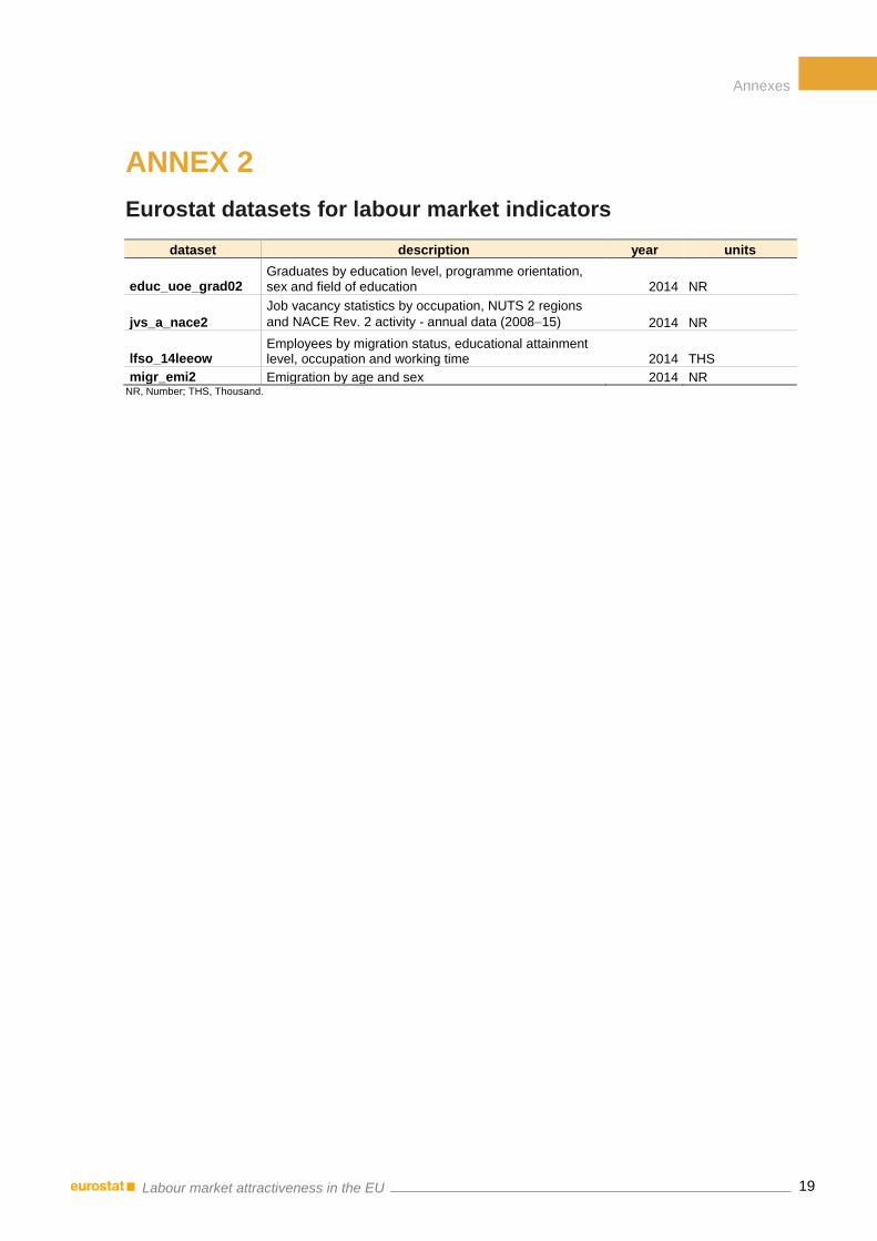
ANNEX 2

Eurostat datasets for labour market indicators

dataset description year units

educ_uoe_grad02 Graduates by education level, programme orientation, sex and field of education 2014 NR

jvs_a_nace2

Job vacancy statistics by occupation, NUTS 2 regions

and NACE Rev. 2 activity - annual data (2008–15) 2014 NR

lfso_14leeow Employees by migration status, educational attainment level, occupation and working time 2014 THS

migr_emi2 Emigration by age and sex 2014 NR NR, Number; THS, Thousand.

Annexes


ANNEX 3

Summary statistics on Labour Market Attractiveness set

variable mean n stdev cv

ARPR 16.84 28 3.822 0.227

AROPE 24.88 28 7.003 0.281

earn_OC[1]_Nace[B–F] 21.99 26 8.169 0.371

earn_OC[1]_Nace[G–N] 21.66 26 7.039 0.325

earn_OC[1]_Nace[P–S] 19.65 26 8.084 0.411

earn_OC[2]_Nace[B–F] 16.68 26 6.406 0.384

earn_OC[2]_Nace[G–N] 16.88 26 5.418 0.321

earn_OC[2]_Nace[P–S] 16.12 26 7.205 0.447

earn_OC[3]_Nace[B–F] 12.73 26 5.018 0.394

earn_OC[3]_Nace[G–N] 13.05 26 4.510 0.346

earn_OC[3]_Nace[P–S] 11.83 26 5.337 0.451

earn_OC[4]_Nace[B–F] 10.54 26 4.248 0.403

earn_OC[4]_Nace[G–N] 10.50 26 3.987 0.380

earn_OC[4]_Nace[P–S] 10.31 26 4.770 0.463

earn_OC[5]_Nace[B–F] 8.36 25 3.722 0.445

earn_OC[5]_Nace[G–N] 8.23 26 3.357 0.408

earn_OC[5]_Nace[P–S] 8.78 26 4.308 0.491

earn_OC[6]_Nace[B–F] 7.34 13 4.668 0.636

earn_OC[6]_Nace[G–N] 8.37 17 3.961 0.473

earn_OC[6]_Nace[P–S] 8.08 16 4.048 0.501

earn_OC[7]_Nace[B–F] 8.84 26 3.997 0.452

earn_OC[7]_Nace[G–N] 8.45 26 3.605 0.427

earn_OC[7]_Nace[P–S] 8.45 23 4.280 0.506

earn_OC[8]_Nace[B–F] 9.07 26 4.024 0.444

earn_OC[8]_Nace[G–N] 8.95 26 3.649 0.408

earn_OC[8]_Nace[P–S] 7.49 23 3.492 0.466

earn_OC[9]_Nace[B–F] 8.01 26 3.601 0.449

earn_OC[9]_Nace[G–N] 7.30 26 3.239 0.444

earn_OC[9]_Nace[P–S] 7.56 26 3.741 0.495

emp_T[F] 47.40 28 5.471 0.115

emp_T[P] 9.55 28 6.764 0.708

emp_Y[15–24] 29.93 28 12.472 0.417

emp_Y[25–64] 70.82 28 5.965 0.084

emp_Y[GE65] 5.72 28 3.010 0.527

emp_Y[15–24]_ED[0–2] 21.51 28 12.135 0.564

emp_Y[15–24]_ED[3–4] 62.21 28 13.026 0.209

emp_Y[15–24]_ED[5–8] 16.02 28 8.998 0.562

emp_Y[25–64]_ED[0–2] 16.40 28 11.835 0.722

emp_Y[25–64]_ED[3–4] 47.84 28 13.232 0.277

emp_Y[25–64]_ED[5–8] 35.41 28 8.727 0.246

emp_Y[15–24]_Nace[A] 6.38 26 8.063 1.264

emp_Y[15–24]_Nace[B–E] 16.60 28 8.450 0.509

emp_Y[15–24]_Nace[F] 6.81 28 2.239 0.329

emp_Y[15–24]_Nace[G–I] 36.75 28 7.242 0.197

emp_Y[15–24]_Nace[J] 2.63 25 1.030 0.391

emp_Y[15–24]_Nace[K] 1.85 17 0.874 0.473

Annexes


emp_Y[15–24]_Nace[L] 0.67 8 0.395 0.592

emp_Y[15–24]_Nace[M–N] 7.47 28 2.254 0.302

emp_Y[15–24]_Nace[O–Q] 14.38 28 6.581 0.458

emp_Y[15–24]_Nace[R–U] 6.50 28 2.265 0.348

emp_Y[25–64]_Nace[A] 5.26 28 4.873 0.926

emp_Y[25–64]_Nace[B–E] 17.43 28 5.650 0.324

emp_Y[25–64]_Nace[F] 6.91 28 1.273 0.184

emp_Y[25–64]_Nace[G–I] 23.32 28 3.717 0.159

emp_Y[25–64]_Nace[J] 3.10 28 0.813 0.262

emp_Y[25–64]_Nace[K] 3.29 28 2.225 0.677

emp_Y[25–64]_Nace[L] 0.81 28 0.498 0.616

emp_Y[25–64]_Nace[M–N] 8.74 28 2.145 0.245

emp_Y[25–64]_Nace[O–Q] 25.62 28 5.179 0.202

emp_Y[25–64]_Nace[R–U] 5.06 28 2.067 0.409

expend_ED[5–8] 1.28 23 0.424 0.333

disp_income 13 323 26 3 736 0.280

GDP 26 839 28 11 430 0.426

GVAgr 1.72 25 1.731 1.009

low_work 10.74 28 3.547 0.330

mat_depriv 10.45 28 7.975 0.763

pop_Total 18 106 210 28 23 370 416 1.291

pop_Y[0–14] 15.71 28 1.802 0.115

pop_Y[15–24] 11.68 28 1.097 0.094

pop_Y[25–64] 54.89 28 2.015 0.037

pop_Y[65–74] 9.59 28 1.098 0.114

pop_Y[GE75] 8.14 28 1.403 0.172

rooms_pp 1.60 28 0.367 0.229

training 10.59 28 8.017 0.757

unemp_Y[15–24] 8.75 28 3.508 0.401

unemp_Y[GE25] 6.19 28 3.320 0.536 n, number of countries; stdev, standard deviation; cv, coefficient of variation.

Annexes


ANNEX 4

Summary statistics on labour market indicators

variable mean n stdev cv

Skills mismatch 59.3 8 20.035 0.338

Mobility 17.92 25 14.384 0.802

Emigration 0.79 28 0.603 0.764 n, number of countries; stdev, standard deviation; cv, coefficient of variation.

Annexes


ANNEX 5

Averages of top 10 separator variables of clusters

cluster GD

P

(x1

03)

ea

rn_

OC

[3]_

Na

ce

[P–

S]

em

p_

Y[2

5–

64]_

Na

ce[K

]

ex

pe

nd

_E

D[5–

8]

ea

rn_

OC

[7]_

Na

ce

[P–

S]

ea

rn_

OC

[5]_

Na

ce

[P–

S]

ea

rn_

OC

[9]_

Na

ce

[P–

S]

po

p_

To

tal

(x1

06

)

dis

p_

inc

om

e

(x1

03)

ea

rn_

OC

[4]_

Na

ce

[P–

S]

AT-BE-CY-MT 28.5 15.3 4.4 1.6 11.6 11.1 9.2 5.2 17.7 12.8

BG-HU-LV-RO 16.0 5.0 2.0 0.8 3.7 3.5 3.1 9.8 8.2 4.5

CZ-SK-SI 22.3 8.2 2.5 1.0 5.6 5.6 4.5 6.0 11.6 7.1

DE-FR-UK 31.2 14.6 3.6 1.5 10.6 10.7 9.3 70.4 18.2 12.5

DK-FI-NL-SE 33.5 15.6 2.9 2.0 13.5 13.5 11.5 9.4 15.7 14.3

EE-LT-PL-PT 20.4 6.7 1.9 1.2 4.9 4.5 4.0 13.2 11.1 5.8

EL-HR 18.0 - 2.6 - - - - 7.6 10.3 -

ES-IT 25.7 12.6 2.8 0.9 9.0 9.5 8.7 5.4 15.1 11.0

IE 36.8 20.2 5.0 1.3 16.3 15.2 14.1 4.6 13.8 18.2

LU 73.0 23.4 13.2 - - 14.8 12.8 0.6 - 19.5

sep = Varb/Varw 34.395 30.24 28.781 20.025 19.772 19.02 17.749 17.176 17.024 14.995 (-) not available.

Varb, Variation between clusters; Varw, Variation within clusters.

Annexes


ANNEX 6

Correlation between labour market indicators and Labour Market Attractiveness

variable Skills mismatch Mobility Emigration

statistic p-value statistic p-value statistic p-value

ARPR 0.33 0.420 -0.09 0.659 0.19 0.322

AROPE 0.38 0.352 -0.25 0.237 0.24 0.223

earn_OC[1]_Nace[B–F] 0.00 1.000 0.34 0.115 -0.07 0.749

earn_OC[1]_Nace[G–N] 0.21 0.610 0.39 0.068 0.02 0.917

earn_OC[1]_Nace[P–S] 0.02 0.955 0.43 0.042 0.14 0.489

earn_OC[2]_Nace[B–F] -0.10 0.821 0.43 0.040 0.08 0.707

earn_OC[2]_Nace[G–N] -0.14 0.736 0.48 0.022 0.10 0.639

earn_OC[2]_Nace[P–S] -0.07 0.867 0.47 0.023 0.22 0.281

earn_OC[3]_Nace[B–F] -0.12 0.779 0.49 0.017 0.14 0.483

earn_OC[3]_Nace[G–N] -0.02 0.955 0.48 0.020 0.10 0.612

earn_OC[3]_Nace[P–S] -0.10 0.823 0.55 0.006 0.24 0.241

earn_OC[4]_Nace[B–F] -0.24 0.570 0.47 0.025 0.10 0.625

earn_OC[4]_Nace[G–N] -0.07 0.867 0.51 0.013 0.16 0.444

earn_OC[4]_Nace[P–S] -0.12 0.779 0.47 0.023 0.24 0.245

earn_OC[5]_Nace[B–F] -0.07 0.867 0.50 0.018 0.08 0.688

earn_OC[5]_Nace[G–N] -0.05 0.910 0.43 0.039 0.10 0.610

earn_OC[5]_Nace[P–S] -0.24 0.570 0.47 0.025 0.18 0.371

earn_OC[6]_Nace[B–F] -0.31 0.456 0.37 0.259 -0.09 0.775

earn_OC[6]_Nace[G–N] -0.21 0.645 0.61 0.016 0.01 0.978

earn_OC[6]_Nace[P–S] -0.03 0.957 0.28 0.334 -0.04 0.888

earn_OC[7]_Nace[B–F] -0.40 0.320 0.48 0.022 0.08 0.709

earn_OC[7]_Nace[G–N] -0.31 0.456 0.45 0.031 0.15 0.454

earn_OC[7]_Nace[P–S] -0.19 0.651 0.43 0.057 0.14 0.529

earn_OC[8]_Nace[B–F] -0.33 0.420 0.43 0.039 0.09 0.677

earn_OC[8]_Nace[G–N] -0.36 0.385 0.55 0.006 0.25 0.225

earn_OC[8]_Nace[P–S] -0.31 0.456 0.53 0.015 0.18 0.422

earn_OC[9]_Nace[B–F] -0.24 0.570 0.49 0.019 0.08 0.699

earn_OC[9]_Nace[G–N] -0.05 0.911 0.47 0.025 0.13 0.537

earn_OC[9]_Nace[P–S] -0.07 0.867 0.46 0.029 0.17 0.399

emp_T[F] -0.57 0.139 -0.23 0.265 -0.28 0.149

emp_T[P] -0.17 0.693 0.57 0.003 0.19 0.343

emp_Y[15–24] -0.76 0.028 0.24 0.254 0.01 0.976

emp_Y[25–64] -0.64 0.086 0.42 0.034 -0.18 0.352

emp_Y[GE65] 0.02 0.955 0.21 0.314 0.16 0.418

emp_Y[15–24]_ED[0–2] 0.24 0.570 0.22 0.291 0.14 0.491

emp_Y[15–24]_ED[3–4] -0.19 0.651 -0.45 0.025 -0.53 0.004

emp_Y[15–24]_ED[5–8] 0.29 0.493 0.37 0.066 0.56 0.002

emp_Y[25–64]_ED[0–2] 0.52 0.183 0.11 0.593 0.34 0.080

emp_Y[25–64]_ED[3–4] -0.29 0.493 -0.38 0.060 -0.52 0.005

emp_Y[25–64]_ED[5–8] -0.33 0.420 0.57 0.003 0.47 0.012

emp_Y[15–24]_Nace[A] 0.36 0.385 -0.34 0.109 0.39 0.051

emp_Y[15–24]_Nace[B–E] 0.31 0.456 -0.58 0.002 -0.56 0.002

emp_Y[15–24]_Nace[F] -0.55 0.160 0.19 0.359 -0.31 0.109

emp_Y[15–24]_Nace[G–I] 0.29 0.493 0.06 0.784 0.22 0.269

Annexes


emp_Y[15–24]_Nace[J] 0.14 0.736 0.17 0.462 0.16 0.434

emp_Y[15–24]_Nace[K] 0.40 0.600 0.25 0.383 0.16 0.535

emp_Y[15–24]_Nace[L] - - 0.64 0.119 -0.17 0.693

emp_Y[15–24]_NaceM_N 0.21 0.610 0.39 0.053 0.08 0.684

emp_Y[15–24]_Nace[O–Q] -0.52 0.183 0.55 0.005 0.04 0.851

emp_Y[15–24]_Nace[R–U] -0.45 0.260 0.53 0.006 0.27 0.171

emp_Y[25–64]_Nace[A] 0.24 0.570 -0.43 0.032 0.13 0.495

emp_Y[25–64]_Nace[B–E] 0.24 0.570 -0.59 0.002 -0.58 0.001

emp_Y[25–64]_Nace[F] -0.50 0.207 -0.11 0.588 -0.34 0.072

emp_Y[25–64]_Nace[G–I] 0.33 0.420 -0.10 0.621 0.18 0.358

emp_Y[25–64]_Nace[J] -0.69 0.058 0.58 0.002 0.07 0.711

emp_Y[25–64]_Nace[K] 0.00 1.000 0.47 0.017 0.38 0.044

emp_Y[25–64]_Nace[L] -0.52 0.183 0.30 0.152 -0.15 0.433

emp_Y[25–64]_NaceM_N -0.19 0.651 0.51 0.008 0.07 0.707

emp_Y[25–64]_Nace[O–Q] -0.21 0.610 0.41 0.040 0.15 0.455

emp_Y[25–64]_Nace[R–U] -0.14 0.736 0.51 0.009 0.23 0.239

expend_ED[5–8] -0.07 0.867 0.40 0.071 0.13 0.561

disp_income -0.07 0.867 0.46 0.028 -0.03 0.885

GDP -0.31 0.456 0.51 0.009 0.10 0.603

GVAgr -0.04 0.939 -0.15 0.496 0.20 0.350

low_work 0.29 0.493 -0.09 0.667 0.06 0.769

mat_depriv 0.45 0.260 -0.49 0.014 0.11 0.565

pop_Total 0.52 0.183 -0.24 0.253 -0.36 0.063

pop_Y[0–14] -0.45 0.260 0.35 0.090 0.23 0.244

pop_Y[15–24] -0.36 0.385 0.13 0.531 0.32 0.097

pop_Y[25–64] 0.10 0.823 -0.31 0.129 -0.03 0.879

pop_Y[65–74] -0.19 0.651 -0.10 0.637 -0.43 0.023

pop_Y[GE75] 0.10 0.823 0.14 0.519 -0.22 0.251

rooms_pp -0.27 0.520 0.55 0.004 0.38 0.046

training -0.35 0.399 0.57 0.003 -0.11 0.576

unemp_Y[15–24] 0.02 0.955 0.00 0.983 0.07 0.711

unemp_Y[GE25] 0.29 0.493 -0.09 0.682 0.07 0.719 (-) Only two datapoints available.

Annexes


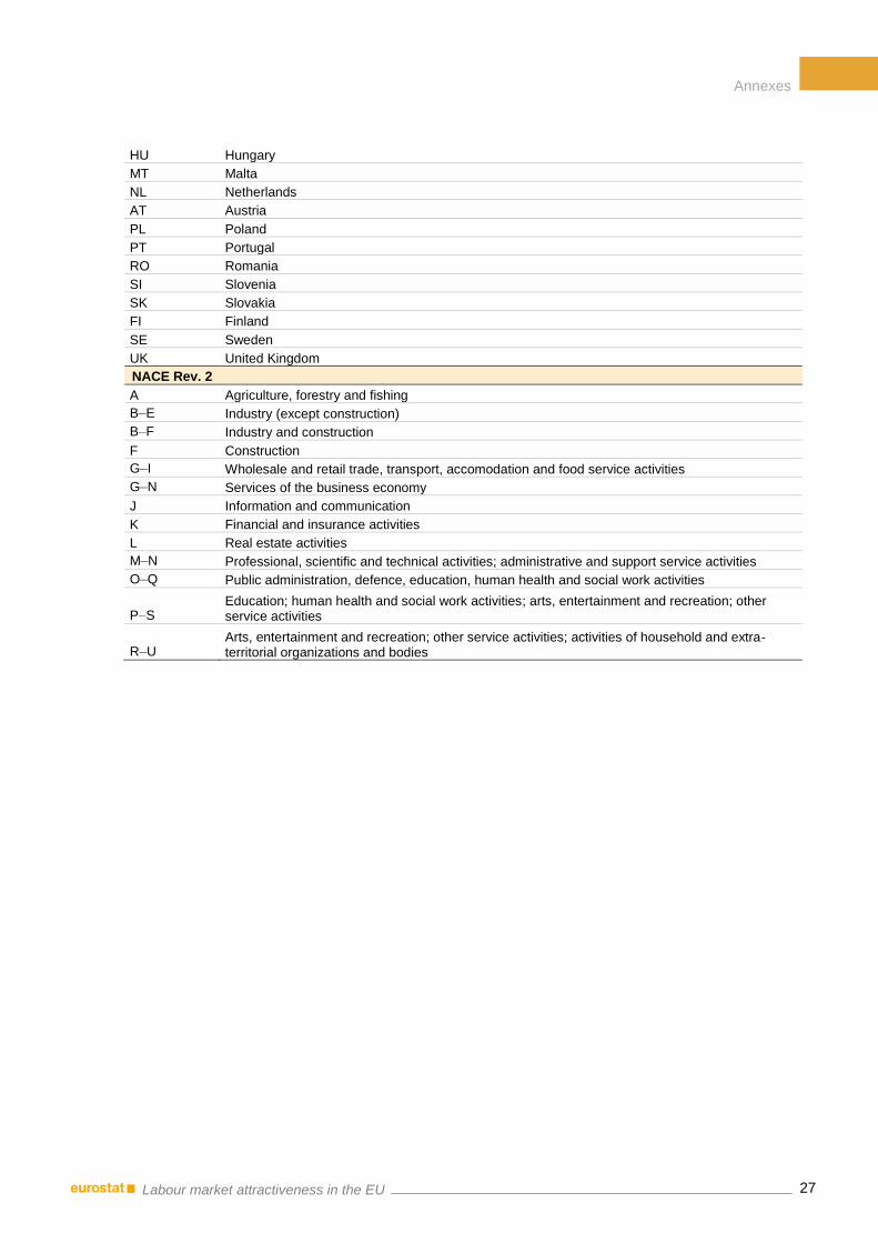
ANNEX 7

Information on ISCED 11 education levels, ISCED-F 13 fields of education, ISCO-O8 job titles, EU-28 countries and NACE Rev. 2 economic activity sectors

ISCED 11

0–2 Less than primary, primary and lower secondary education

3–4 Upper secondary and post-secondary non-tertiary education

5–8 Tertiary education

ISCED-F 13

00 Generic programmes and qualifications

01 Education

02 Arts and humanities

03 Social sciences, journalism and information

04 Business, administration and law

05 Natural sciences, mathematics and statistics

06 Information and Communication Technologies (ICTs)

07 Engineering, manufacturing and construction

08 Agriculture, forestry, fisheries and veterinary

09 Health and welfare

10 Services

99 Unknown

ISCO-08

0 Armed forces occupations

1 Managers

2 Professionals

3 Technicians and associate professionals

4 Clerical support workers

5 Service and sales workers

6 Skilled agricultural, forestry and fishery workers

7 Craft and related trades workers

8 Plant and machine operators and assemblers

9 Elementary occupations

EU-28

BE Belgium

BG Bulgaria

CZ Czech Republic

DK Denmark

DE Germany (until 1990 former territory of the FRG)

EE Estonia

IE Ireland

EL Greece

ES Spain

FR France

HR Croatia

IT Italy

CY Cyprus

LV Latvia

LT Lithuania

LU Luxembourg

Annexes


HU Hungary

MT Malta

NL Netherlands

AT Austria

PL Poland

PT Portugal

RO Romania

SI Slovenia

SK Slovakia

FI Finland

SE Sweden

UK United Kingdom

NACE Rev. 2

A Agriculture, forestry and fishing

B–E Industry (except construction)

B–F Industry and construction

F Construction

G–I Wholesale and retail trade, transport, accomodation and food service activities

G–N Services of the business economy

J Information and communication

K Financial and insurance activities

L Real estate activities

M–N Professional, scientific and technical activities; administrative and support service activities

O–Q Public administration, defence, education, human health and social work activities

P–S Education; human health and social work activities; arts, entertainment and recreation; other service activities

R–U Arts, entertainment and recreation; other service activities; activities of household and extra-territorial organizations and bodies

Getting in touch with the EU

In person

All over the European Union there are hundreds of Europe Direct Information Centres. You can

find the address of the centre nearest you at: http://europa.eu/contact

On the phone or by e-mail

Europe Direct is a service that answers your questions about the European Union. You can

contact this service

– by freephone: 00 800 6 7 8 9 10 11 (certain operators may charge for these calls),

– at the following standard number: +32 22999696 or

– by electronic mail via: http://europa.eu/contact

Finding information about the EU

Online

Information about the European Union in all the official languages of the EU is available on the

Europa website at: http://europa.eu

EU publications

You can download or order free and priced EU publications from EU Bookshop at:

http://bookshop.europa.eu. Multiple copies of free publications may be obtained by contacting

Europe Direct or your local information centre (see http://europa.eu/contact)

EU law and related documents

For access to legal information from the EU, including all EU law since 1951 in all the official

language versions, go to EUR-Lex at: http://eur-lex.europa.eu

Open data from the EU

The EU Open Data Portal (http://data.europa.eu/euodp/en/data) provides access to datasets from

the EU. Data can be downloaded and reused for free, both for commercial and non-commercial

purposes.

http://europa.eu/contact


http://europa.eu/

http://bookshop.europa.eu/


http://eur-lex.europa.eu/

http://data.europa.eu/euodp/en/data

How

does attrition affect persistent poverty rates ? The case of EU-SILC

2018 edition


In this work we present a framework developed for the European Big Data Hackathon 2017. This framework is divided in two parts: an exploration part, which is aimed to better understand the EU global labour market and to capture its heterogeneity; and an inferential part, whose goal is to establish associations between characteristics of the EU labour market and indicators designed to capture important aspects of the labour market (i.e. Skills mismatch, Mobility and Emigration). For the exploration part, we developed the concept of Labour Market Attractiveness, which consists of a combination of socio-economic and demographic variables from Eurostat datasets. Using data mining techniques, such as social networks and clustering analysis, we showed that this combined set consistently captured the country-level heterogeneity in the EU, forming well-defined clusters. For the inferential part, we used model selection analysis and weighted network correlation analyses to establish associations between the characteristics of the EU labour market and the labour market indicators. We argue that the combination of both exploration and inferential parts can disentangle the complex dynamics of the EU labour market and help setting effective policies to tackle typical problems of a fast-changing global labour market environment.

For more informationhttp://ec.europa.eu/eurostat/

KS-TC-18-002-EN-N

ISBN 978-92-79-80731-2

http://ec.europa.eu/eurostat/

labour market attractiveness in the...

Documents