Lefebvre : Université du Québec à Montréal and CIRPÉE

lefebvre.pierre@uqam.ca

Merrigan : Université du Québec à Montréal and CIRPÉE

merrigan.philip@uqam.ca

Corresponding authors: Pierre Lefebvre/Philip Merrigan, Department of Economics, UQAM, CP 8888, Succ. Centre-ville, Montréal, QC, Canada

H3C 3P8

The analysis is based on Statistics Canada’s Youth in Transition Survey (YITS) restricted-access Micro Data Files, which contain anonymized

data collected in the YITS and are available at the Québec Inter-university Centre for Social Statistics (QICSS), one of the Canadian Research

Data Center network. All computations on these micro-data were prepared by the authors who assume the responsibility for the use and

interpretation of these data. We thank Anne Motte and an anonymous referee for their comments and useful suggestions on the first version of

this paper. This research was funded by the Canada Millennium Scholarship Foundation.

Cahier de recherche/Working Paper 10-45

Labour Outcomes of Graduates and Dropouts of High School and

Post-secondary Education: Evidence for Canadian 24- to 26-year-olds

in 2005

Pierre Lefebvre

Philip Merrigan

Novembre/November 2010

(First version November 2009, revised January 2010)

Abstract: The purpose of this research is to estimate the impact of education, with a particular focus on education levels lower than a university diploma, on the labour market and social outcomes of the 24- to 26-year-old Canadians found in the fourth wave of the Youth in Transition Survey (YITS), conducted by Statistics Canada in 2006. We focus on differences between individuals who did not pursue college or university level degrees. We find that dropouts perform very poorly for most of the outcomes we analyse. Our most important result is that males who finish their high-school degree very late (after 19 years of age), perform, ceteris paribus, at many levels like dropouts. This suggests that policy makers should be taking a very close look at “second chance” or “adult education” programs across Canada. Keywords: Education levels, high school and postsecondary dropouts, graduate and continuers, earnings, wage rates, employment, employment insurance and social assistance, volunteer activities, youth skills

JEL Classification: I21, I28

2

1. Introduction

The purpose of this research is to estimate the impact of education, with a particular focus on

education levels lower than a university degree or college diploma, on the labour market and social

outcomes of the 24- to 26-year-old Canadians found in the fourth wave of the Youth in Transition

Survey-Cohort B (YITS-B), conducted by Statistics Canada and which concerns the period of

January 2004 to December 2005. Most of the literature on the impact of education is concerned

with the gaps between individuals with only a high school diploma and a university degree (BA).

However, as observed by Boothby and Drewes (2006), about two-thirds of those with a

postsecondary education (PSE) acquired such education outside universities (such as community

colleges, trade institutions, or other vocational programs). Rising tuition fees and supply

constraints (availability of university “seats”) in the 1990s according to Fortin (2005) and Fortin

and Lemieux (2005) have limited educational achievement and increased returns to university

education. This educational policy may have induced potential university students to consider PSE

outside universities where the fees are generally lower. We provide estimates of early labour

market outcomes for different levels of education obtained across different educational settings.

Although respondents in cycle 4 of the YITS are young (24-26 years) in terms of life-cycle

labour supply decisions, we can get a good sense of who gets the better start after the completion

of schooling. Surprisingly, our results show that even at such a young age, important differences

exist between individuals with varying levels of education. In this respect, the YITS is an excellent

data set to address this issue. First, we observe very detailed information on the type of degrees or

diplomas respondents receive, if any. Second, the information on labour supply is plentiful as the

following variables are available in the survey: the months of work experience from ages 18 to 26,

hourly wages, annual earnings, number of jobs, and training. Finally, the YITS provides the age at

which a high school diploma was received, a very important piece of information, as we shall see

later, as well as a host of socio-demographic variables available for regression analysis.

The specific objective of the paper is to estimate the impact of different levels of education on

labour and social outcomes and in particular for those individuals with lower educational

attainments. We classify, for the purposes of regression analysis, levels of education into six main

groups: 1) university graduates; 2) college graduates; 3) graduates from a diversity of post-

secondary education (PSE) programs different from programs leading to a college diploma (trade,

vocational, apprenticeship) with a high school diploma; 4) high school (HS) graduates with some

3

partial PSE education and without a diploma or certificate (they can be considered as PSE or

university dropouts); 5) HS graduates (with HS only or an equivalency); and, 6) HS dropouts (no

HS diploma). In another set of regressions, we replace these classes (but use the same control

variables) with an alternative classification based on the age of graduation from HS (four

categories are constructed: individuals who graduated between 15 and 19 years of age, 20 and 26

years of age, age of graduation not stated, and no HS diploma). All regressions are performed by

gender as males and females face different labour markets and occupy different types of jobs.

There are several reasons why our analysis concentrates on low-education groups. First, we

seek to determine whether an individual whose highest educational attainment is a HS diploma has

better job market prospects than a dropout. It will be difficult to make the case for public policies

aimed at increasing high school graduation rates if this is not the case. Second, comparing those

who obtain their HS diploma at a late juncture, probably in adult education or “second chance

education”, with HS dropouts, will inform us as to the value of these diplomas relative to dropping

out. We want to compare young Canadians with young Americans in the United States, where

Heckman and Lafontaine (2008) find that, controlling for skills, individuals with a General

Equivalency Diploma or “GED” have similar wages to dropouts. This is an economically

important question as provincial governments spend considerable amounts of money in these

“second chance” programs. Individuals may also be losing valuable experience on the job market

participating in these programs. If we find that these programs are inefficient, some type of

overhaul should be considered by provincial governments.

The labour market outcomes are classified into four main groups: 1) employment; 2) receipt of

social assistance or Employment Insurance (EI) benefits in year 2005; 3) annual earnings in 2005

and wages rates of last job; 4) employer and career training1. A final social outcome is analysed:

volunteer activity and the frequency of such activities. These activities may be indicative of social

and civic engagement by the respondent.

The paper is structured as follows: section 2 reviews recent research on the topic of education

and its impacts on different outcomes. Section 3 and 4 present respectively the data from the

YITS, labour market outcomes, and explanatory variables. Section 5 presents the characteristics

1 We consider that individuals who answered yes to: “Not including any schooling or training already discussed, in the

last two years, have you attended other courses or training programs related to a job or career?” received career

training . Individuals who answered yes to the question: “Did you participate in any courses or training programs

organized by any of your employers in the last two years?” are considered to have received employer training.

4

and labour market outcomes of youth by gender and level of education by December 2005. The

results from multivariate regressions are discussed in section 6. Section 7 offers policy

implications and concludes with a summary and some final observations.

2. Review of recent research

Most of the Canadian research on education outcomes has emphasized returns and used Census

data. Updating an earlier 2006 study, Bourdarbat et al (2008), rely on 1981 to 2001 Census files to

estimate the skill premium, measured in weekly earnings and adjusted for experience, for the 16 to

65 age group full-time workers, and for seven educational levels. For men, they find a large (40%)

wage gap between university and high school graduates which increased steeply between 1995 and

2000, and that the return to education for young men also grew substantially during the 1980s and

early 1990s, in contrast to other evidence suggesting stable returns over the last two decades. The

two education levels below HS, (some years of education and some HS) have negative returns (10-

20%) relative to a HS diploma. The returns for the two education levels above HS ((1) some

postsecondary education; (2) a postsecondary degree) have low returns compared to HS

(respectively 5% and 15%) but are slowly increasing over time. The supplementary return for

postgraduates over BA graduates is around 10% with marginal changes over the years.

For women, the returns to education – as measured by the skill premium relative to high school

graduates - are systematically larger than for men; and most wage differentials due to education

among women have been relatively constant over time. The return to high school completion has

remained stable, as is the case for men. The two education levels below HS (some years of

education, some HS) have higher negative returns (15-25%) relative to a HS diploma than for

men. The returns for the two education levels above HS have also higher returns compared to HS

(respectively 15% and 18%, higher than for males) but are rather flat over time. The

supplementary return for postgraduates over BA graduates is around 15% and slightly increasing

over the years. The wage gaps adjusted for experience are larger, especially for men, highlighting

the importance of controlling for others factors in wage regressions.

But the existing education literature has provided few estimates of the returns to post-secondary

non-university education from a community college or through a trade diploma, and even less for

the returns to apprenticeship training (Gunderson, 2009). Gunderson and Krashinsky (2005) use

5

the 2001 Canadian census to estimate an average return of 3.9% for each year of basic education

acquired by an individual plus an additional return for completing key phases of education. For

completing a trade certificate over and above completing high-school, the returns averaged about

3%, although they were negative for females (-3.4%) and positive for males (5.5%).

Boothby and Drewes (2006) use the 1981, 1991 and 2001 Canadian censuses and also find

small earning premiums for those with a non-university PSE (community colleges, trade

institutions, and other vocational educations) compared to high school graduates, with the

premium being smaller for females than for males. The premium increased, however, for

individuals with both a trade certificate and a high school degree (1980 to 1985). But the earnings

premiums are substantially lower than the earnings difference between high school graduates and

university graduates (Bachelor's degree). Ferrer and Riddell (2002) use the 1996 Canadian census

and estimate rates of return of approximately 8% annually for completing a community college or

a trade diploma compared to HS; the difference between HS graduates and HS dropouts is around

12-16%, while the earnings difference between HS graduates and university graduates is

significantly higher, between 36-47%.

The only published study to our knowledge specifically on college graduates from community

colleges or CEGEPs, is Boudarbat (2008) who uses the National Survey of Graduates (NSG) for

years 1990 and 1995 and analyses their earnings two years after their graduation retaining those

aged 16 to 65 years (!). They are categorized in five fields of study and prospective gains are

calculated by field of study. It is not clear which graduates are retained in terms of education

programs (technical, trade, vocational?) in this study.

Hansen (2006), with the same NSG surveys, analyses wage differences between university

graduates and college graduates (including those from trade schools). He also examines wage

differences between individuals on the basis of their field of studies, and type of industry the

respondent reports for his job as well as his occupation. He finds that the ceteris paribus

differences in earnings based on the type of degree have decreased from 1992 to 2002 for both

males and females. Furthermore, he uses the Census Public files of 1991 and 2001 to compute the

internal rate of return for university education (by type of studies and region) relative to a

secondary level of education. He finds that the rate of return has slightly increased from 9 to 11%

across all fields and regions.

6

Hansen (2007), with cycle 3 of the YITS, analyses the earnings difference between post-

secondary graduates and high-school graduates by region (4) as well as differences between post-

secondary graduates according to their field of study (7) and their occupations (4). Other

dependent variables are analyzed such as schooling interruptions and the regional mobility of

graduates. The results demonstrate that those who have a high school diploma do better than

dropouts. A strange result is that « Low-PSE » (lower than university) graduates do better than

« High-PSE » (university graduates). This could be due to the very young age of the respondents

in cycle 3 of the YITS (22 to 24). In other words, recent university graduates are at a lower point

on their age-earnings profiles – because they are recent graduates – but will catch-up and surpass

college graduates. Education effects are found to be stronger for females.

Using cycle 3 of the YITS-cohort-B (aged 22-24 in December 2003), Campolieli et al. (2009)

examine fifteen outcomes (from wages to employment, to subsequent skill acquisition and to

job/pay satisfaction) for dropouts who are compared to high school graduates who did not pursue

postsecondary education. With respect to the determinants of dropping out (from a first stage of

their analysis to calculate an instrumented dropout variable), they find no gender effect (which is

surprising; provinces are control variables but their estimated parameters are not presented). They

find that dropping out of HS compared to having only a HS diploma is associated significantly

with a much lower probability of being employed (18 points lower), of having a stable job (19

points lower), of a lower starting and ending wage in the first job, of lower wages in their final job

and of a lower probability of job training. Dropouts do not seem to be “able to compensate or

substitute for their lack of formal education by acquiring skills through subsequent training” (page

13, Campolieli et al.).

Influential results, presented by Oreopoulos (2005, 2006, 2007) who uses compulsory

schooling laws that force students to take an extra year of school experience, indicate that this

extra year of schooling will increase annual earnings on average by 10 to 12% as well as generate

significant benefits for health, employment, decreasing poverty, and raise subjective measures of

well-being.

Concerns about high-school dropouts regularly dominate policy discussions in the field of

education. Analysts focus on interventions that will provide incentives for dropouts to eventually

return to school and obtain their high-school diploma or the equivalent. However, little is known

about the returns of such policies that can be costly for governments. A substantial proportion of

7

high school graduates in Canada obtain their high-school diploma by way of equivalencies. The

exact number of young adults who obtain their diploma this way is difficult to ascertain but in the

YITS at least 4.2% of females and 5.3% of males obtain their diploma between the ages of 20 and

26.

There is some recent evidence in the United States which shows that focusing on high school

graduation rates as a measure of a successful education policy could be a mistake. In some recent

work, Heckman and Lafontaine (2006, 2008, 2008a, 2008b) and Cameron and Heckman (2003)

demonstrate that high school certificates that are named GEDs (i.e. are obtained by equivalencies)

have a questionable value in the labour market:

“A substantial body of scholarship summarised in Heckman and LaFontaine (2008) shows that

the GED program does not benefit most participants, and that GEDs perform at the level of

dropouts in the U.S. labour market. The GED program conceals major problems in American

society.” Heckman and Lafontaine (2008)

The papers show that once regression analysis controls for measures of IQ when the child is

young, GED graduates sometimes actually do worst in the labour market than dropouts having

never received a high school diploma or the equivalent. This result sheds some doubt on the value

of these GEDs. Given their costs, governments may reconsider their investments in this area or try

to increase the value of GEDs.

We can closely observe the educational choices of young adults in Canada with two

comprehensive data sets: the Youth in Transition Survey (YITS) and the National Longitudinal

Survey of Income and Youth (NLSCY) which is not used in this paper. The YITS-B cohort (18-20

years old in 1999) is observed at four different time periods separated by 2 years. In cycle 4,

respondents are 24 to 26 years old. Therefore, it is possible to observe those who do not graduate

by the age of 20 for 4 to 6 years and reveal how they finally obtain their high school diploma. It is

also possible to measure how well they are doing in the labour market when compared to actual

dropouts. In particular, we will be performing probit regressions of employment on education

(high school graduation before the age 20 versus graduation between ages 20 to 26 versus

dropouts) and other characteristics; in particular measures which proxy skill levels (Heckman and

Lafontaine use IQ). Other outcomes are labour market earnings and wages with estimations

performed by OLS or Tobit. As mentioned in the introduction, if conditional on skills, adult

8

education individuals do not perform better than dropouts, some serious doubts about the efficacy

of such programs can be entertained.

Hansen (2006, 2007) examines “early” graduates (the 2007 paper uses data from cycle 3 of the

YITS; the 2006 paper used the National Graduates Survey and examines earnings differences

between college and university graduates across disciplines) and their labour market outcomes by

education level (and field of study and occupation) but does not tackle the question of the efficacy

of educational attainments at a finely disaggregated level or of “GEDs”.

In summary, Canadian studies have shown the existence of significant earnings premium

associated with university graduation compared to high school graduation. However the earnings

gains progression associated with acquiring education beyond high school and below a university

bachelor’s degree is less documented for young adults. Nonetheless the Canadian postsecondary

non-university education system offers a large diversity of programs from the special CEGEP

college tracks in Québec to heterogeneous community colleges in the rest of Canada and trade

schools (see below for the education status of youth below the university level). Moreover, many

students do not obtain a PSE certificate. Thus, it is important to study early labour market

outcomes of youth having less schooling than a university degree.

A large number of papers in the last thirty years show that education has a significant private

direct life-time effect on earnings. However, other dimensions of the effects of education should

be considered. For example, Hansen (2006) shows that the probability of being unemployed is

significantly lower among male university graduates than among trade school/college graduates in

the nineties. The experience of unemployment or non-employment may entail that society has to

support through employment insurance or social assistance the less educated. Spells of

unemployment and non-employment or social assistance reduce labour market experience and

therefore decrease life-time income, even if their earnings are relatively modest. It is also possible

that education creates other benefits to society that are not reflected in the earnings of the

educated. Some studies (Oreopoulos, 2007; Moretti et al., 2004) find that students with additional

schooling experience, besides substantial gains to lifetime wealth and better health, are less likely

to be either depressed, looking for work, be in a low-skilled manual occupation, or unemployed.

Adults with more schooling are also more likely to report being satisfied overall with the life they

lead, and are better citizens (in terms of participation and involvement in political life).

Mis en forme : Retrait : Première ligne: 0 cm

9

3. Data set and education status

The YITS data set

The analysis is based on the 12,435 cohort-B respondents interviewed in cycle 4 of the YITS.

They are aged from 24 to 26 as of December 31 2005. After excluding deceased respondents,

those residing in the United States and a few not residing in any of the ten provinces, 12,259 youth

were categorised according to ten education levels as derived from the variables related to high

school and post-secondary status in the survey.

Educational attainment and attendance

The YITS includes many variables on the education status of respondents from which we

derive their education level. The first one is the individual’s high school status as of December

2005 (graduate, leaver, continuer, not stated). Very few persons are high school continuers (55)

because individuals are aged 24 to 26. A second variable identifies the highest certificate, diploma

or degree obtained as of December 2005, from a high school diploma or equivalent to a Ph. D.

degree.2 Two other variables specify on the one hand the highest education level attended as of

December 2005 (less than a high school completion, high school graduation, some post-secondary

education – certificate, and graduation from a post-secondary program),3 and, on the other hand,

the highest level of post-secondary education attended4 across all programs and institutions as of

December 2005, from attestations of a vocational specialisation, to a registered apprenticeship

program, college program straight up to a Ph.D. degree.5 Again, some youth who have graduated

2 About one hundred respondents have a degree, certificate or license from a professional association (accounting,

banking, or insurance) and other levels of post-secondary education (a very general category). 3 For this variable, a little less than 500 respondents are categorized as not stated.

4 The universe of this variable also includes respondents who may have graduated from this level, may still be in a

program, or may have left a program. 5 Approximately 250 respondents had taken a diploma, certificate or license from a professional association

(accounting, banking, or insurance) and the unspecified other levels of post-secondary studies (a very general

category).

10

from high school declared that they have attended a PSE program but their program is not stated

(we classified them as HS graduates with a non-stated PSE status).

The levels of education derived from these four variables are presented in the first panel of

Table 1. Although ten education levels can be identified, in the main estimations only seven levels

of education are used. The continuers (in university, college, other PSE programs, or HS) are

excluded because as of December 2005 they are classified as attending a PSE program or HS. In

some estimations are also excluded the small group of HS graduates who have obtained or have

attended some PSE programs but cannot be classified because their status is in the not-stated

category for all education variables. The ten groups (1a, 1b, 2a, 2b, 3a, 3b, 3c, 4a, 4b, 5) are the

following by level:

1) University level: a) graduates with a bachelor’s degree or graduate-level diploma, certificate

or degree; b) continuers (some may have already a bachelor’s degree or a higher degree,

diploma or certificate).

2) College level: a) graduates (college or CEGEP diploma, university diploma lower than BA

or certificate below bachelor’s degree); b) continuers.

3) Other post-secondary education (PSE) level: a) PSE graduates from a private business or

training institute, or with a trade certification (all having a high school diploma); b) high school

graduates who have pursued college or other PSE studies and can be considered as dropouts of

these programs; c) high school graduates who have a different degree, diploma or certificate

than college and are continuers.

4) High school level: a) high school graduates who have not pursued any other studies as of

December 2005; b) and high school graduates who have graduated from any PSE program or

have taken any type post-secondary education as of December 2005.6

5) Less than high school (high school dropouts). These youth have not completed their high

school diploma (or equivalency) and have not taken any post-secondary education as of

December 2005. Some (55) were high school continuers as of December 2005 and according to

the other education variables are considered as college graduates (2) and dropouts (49). The

number of high school dropouts is smaller than the number of leavers given by the variable

high school status, because some have benefited from “first/second” chance programs and have

pursued or obtained a PSE certificate, diploma or degree as of December 2005. They are

categorized in the preceding education categories.

6 These youth, approximately 500 respondents are in the not-stated category for all the variables, except the high

school status variable. We decided to keep them in a separate category instead of dropping them of the sample. But in

some estimation they were excluded since results for this category were difficult to interpret compared to the others

(see descriptive statistics for this group).

11

Finally, 14 respondents could not be classified (they received the “not stated” status for all the

education variables) and were dropped from the sample. Thus, 12,259 respondents (6,263 females

and 5,996 males) can be potentially used for estimations, including 2,693 respondents (1,428

females and 1,265 males) who by December 2005 are attending an education program. In the

estimations, we exclude continuers, ending up with a sample of 4,835 females and 4,731 males,

abstracting from missing information for explanatory variables, reducing the number of

observations in the regressions.

Table 1 presents the percentage of individuals for each of the ten levels of education by gender,

for Canada and by region of residence in cycle 4 of the YITS. A striking fact is the gender gap in

educational attainment. Females have higher levels of education than males in all regions and are

much less likely to be high school dropouts. For Canada, and almost all provinces, more than fifty

percent of females have obtained or pursue a university degree or college diploma, the exceptions

being Manitoba-Saskatchewan and Alberta. For Canada more than fifty percent of youth (females

or males) have obtained or pursue a non-university PSE education. The percentage for university

PSE education is much lower (30% for females and 21% for males). Females are also more likely

to be continuers in university and college programs. Residents of Québec, in particular males, are

more likely than in the other provinces to be in the college education category, which can be

explained by the role of colleges in the PSE education system (technical college diplomas are

offered in CEGEP, and a CEGEP college diploma - technical or general - is compulsory for

university admission). A rather large proportion of individuals (around 25%) have a lower than

university or college PSE education status. At this level, except in Québec, males are more likely

to have a high school diploma and be considered as continuers at some level of education. Around

10 to 12% of individuals with a high school diploma can be considered as dropouts of PSE

education (i.e. those with a high school diploma with partial studies at the PSE level category). In

Canada, 11% of females and 17% of males surveyed in cycle 4 of the YITS have only a HS

diploma and no higher certificates or degrees. These proportions are higher in some provinces, in

particular in Manitoba-Saskatchewan and Alberta and for males. The percentage of “high school

dropouts” is different than the percentage with no high school diploma because some of these have

a PSE credential and are therefore not included in the high-school dropout category.

Age at high school diploma

12

The “age at which a youth obtained a high school or equivalency certificate (HS)” variable was

used to create an alternative educational status variable for regression purposes. Four variables

were derived from it: 1) Graduated HS between the ages of 15 and 19; 2) Graduated from HS

between the ages of 20 and 26; 3) HS degree but no stated age of completion, according to

information collected in cycles 3 and 4; 4) No HS degree (nonetheless some respondents have

declared receipt of a PSE diploma, certificate or degree). The bottom panel of Table 1 presents the

percentage in each category. A very large percentage of youth completed their HS diploma

between ages 15 and 19. Again, there is a gender gap: males are less likely to obtain a HS diploma

between ages 15 and 19 and they are over-represented in the group receiving their diploma

between 20 to 26 years of age. Finally, very few respondents still pursue a HS diploma at ages 24

to 26 (most are men), and males are much more likely than females to be HS dropouts.

4. Labour market outcomes and explanatory variables

Labour market outcomes

The YITS contains a large diversity of information related to the labour market over cycles 1 to

4 of the survey. We retained labour market outcomes derived in cycle 4, as a large number of

youth are no longer enrolled in education programs and have joined the labour market. Earlier

labour market outcomes are much more delicate to interpret as a large majority of youth are

simultaneously holding a part-time or full-time job (in particular in the summer months) while

enrolled full-time or part-time in education programs. Table 2 presents outcome measures used as

dependent variables. Eight outcomes are studied: (1) the probability of being employed in

December 2005; (2) the probability of receiving EI benefits in 2005; (3) the probability of

receiving social assistance in 2005; (4) annual earnings in 2005; (5) hourly wages; (6) monthly

wages; (7) the probability of career and employer training; (8) the probability and intensity of

participating in volunteer activities. These outcomes are analysed by education level in a

regression context.

Explanatory variables

Regressions are performed with two sets of explanatory variables based on education. The first

set is based on educational attainment and corresponds to seven of the ten categories enumerated

13

in the sub-section “Educational attainment and attendance” in Section 4. We use seven categories

because we exclude continuers from the regression samples. Our goal is to estimate the impact of

education for those who are not in school. These included categories are: University graduate,

College-Graduate, PSE-trade, PSE-part-HS, High-school-other (not-stated PSE program), High-

School-other, and Dropout (See Table 3, for definitions). Certain regressions exclude from the

sample the respondents from the High-school-other as the interpretation of the coefficient is not

clear. Because we include a constant in all regressions, we must exclude one of the seven

categories, we chose University-Graduate which becomes the reference category. A second set of

regressions is based on education variables which depend on the age of graduation. In this case we

have four categories, HS age 15-19 years, HS age 20-26 years, HS age not stated, and Dropout

(see Table 3, for definitions). Again, a constant is included in the analysis; therefore we exclude

the Dropout variable, the reference category.

We also perform some regressions with what we call a low education sample. We do this

because we believe that the wage structure could be different for the low education group. Hence

we exclude University and College graduates because they face a different labour market. Also,

unobserved skills are (arguably) higher amongst college and university graduates. This sample

should reduce problems associated with unobserved “skills heterogeneity”. In this case, when we

use educational attainment variables as regressors, we include 4 categories (or 3 sometimes

leaving out High-school-other because it is not significant). The reference category is chosen to be

High-School-other. The same 4 “education” variables as in the full sample appear for the low-

education sample regressions based on age of HS graduation.

Finally, we sometimes contrast samples based on the number of months respondents have been

out of school. In general, the gap between high and low education students is higher when more

time has expired since leaving school. Therefore, one sample is composed of students who have

left school 6 months or sooner before the survey while the other uses a 12 month cut off.

The first basic group of control variables other than education are: age and province of

residence. The second group consists of background characteristics: having a child, household

structure (couple, single, other), citizenship by birth, language (English, French, English and

French), visible minority, urban status, work limitations, and a social support scale. The third

group of variables refers to the youth’s self-reported skills (computer, writing, reading,

communication, problem solving, and math). These skill variables are very important for our

14

comparisons of dropouts with individuals who received their high school degree in the second

chance system. Indeed, we wish to compare them on the basis of similar skill levels, as in

Heckman and Lafontaine, with dropouts. Two other variables appear as regressors: number of

months having a job (computed over the months from January 1999 to December 2004) and

number of months the youth was a full-time student, at the high school or postsecondary levels

(January 1999 to December 2005). The experience variable is crucial as dropouts, for example,

should have more experience on average than university graduates.

15

5. Characteristics of youth, occupations and industries by level of education and gender

Table A1 presents the characteristics and labour outcomes of respondents by gender for the

seven levels of education, with a sample including the youth with a HS diploma and unstated PSE

education, finished or attended by December 2005, and excluding continuers (university, college,

PSE, HS). What is most remarkable is the strong link between characteristics and educational

attainments: university graduates are less likely to have children, to be citizens by birth, more

likely to be part of a visible minority, more likely to have English and French as reported

language, to live in an urban setting, less likely to have work limitations, have a much higher score

on the social support scale, have higher skills and have accumulated much higher student months

and also accumulated more working months. HS only graduates and HS dropouts present less

favourable characteristics on all dimensions. Females are also different from males for all

educational attainments: they are more likely to live with a child, in particular if they have a lower

educational attainment, are less likely to be part of visible minority, to live in an urban setting,

more likely to have work limitations, have a higher score of social support, and have higher skills

in writing, reading and oral communications.

Labour outcomes are also correlated with education levels: earnings, wage rates and monthly

wages of university and colleges graduates are much higher than those with lower educational

attainments. The disparities for males compared to females is less severe since they have

accumulated more working months (experience) and females are much more likely to have a child

and be out of the labour market (as is indicated by the probability of having a job on December

2005). The probability of having received employment insurance during year 2005 is correlated

with education: the lowest rate of 9% is for male university graduates and it increases with the

lower educations levels, reaching 17 to 19% for males having a HS only or being a HS dropout

(the higher rates for females may be partly explained by the likelihood of having giving birth). A

small proportion has received social assistance during 2005. But the rates increase sharply for

lower education levels, in particular for females. Employer and career training are prevalent

phenomena for all education levels but those with the lowest rates are the less educated. Finally,

volunteering activities are more likely pursued by females and by those having higher education

levels.

Mis en forme : Interligne : 1,5 ligne

16

The last panel of Table A1 presents the same statistics by the age of completion of the high

school diploma. The same pattern of differences in characteristics and labour outcomes can be

observed between the four groups (HS between 15-19 years, HS between 20-26 years, HS age not-

stated, and Dropout).

Table A2 presents the two digit code7 occupations (10) and industries (16) of the respondents

having declared an eligible job in cycle 4 (it is the last job declared that we retain)8 for the ten

levels of education and by gender. Continuers (university, college, PSE, HS) and dropouts are

much more likely to declare no job. Surprisingly a small percentage in all education categories

report having a management occupation. A large proportion of youth, especially females, declared

a job associated with business, finance and administration, for all educational levels, except

dropouts. Occupations associated with health are also the domain of females with very few having

a HS only diploma or no HS diploma. The occupations in the social sciences, education and

government are largely occupied by the university graduates or continuers. The sales and service

occupations are dominated by education levels below university, especially the lower levels which

are predominantly occupied by females. The main occupations for males with low levels of

education are those associated with trade, transport and equipment operation.

For the industries where individuals are employed, the university level youth are concentrated

in the education services, the professional, scientific and technical services, the trade services, and

public administration. A traditional division by gender can be observed: females are more present

in the education services, health care, and social assistance sectors as well as the accommodation

and food services sector where youth with lower education levels are overrepresented. Males with

lower education levels are predominantly in the construction, manufacturing, trade, transportation

and warehousing, and primary sectors.

6. Econometric results

We present all estimated models with the same set of control variables and by gender. For each

dependent variable, the regressions are performed with different samples. The first includes all

individuals who are out of school (non-continuers); the second excludes from the first those who

were not full-time students in the past 6 months while the third excludes those who were not full-

7 There were not enough respondents to adopt a four digit classification.

8 Up to 7 jobs can be reported over the period Jan04-Dec05, but most respondents (52%) report one job, 29% report a

second job, 13% a third job, 5% a fourth job, and the rest (2%) between 5 and 7 jobs.

17

time students over the last twelve months. The latter samples are constructed so that they are

composed of students who had some time to look for work and get their feet wet in the labour

market. These three samples are sometimes reduced by excluding university or college graduates.

Employment outcomes

We start with the results for the probability of being employed in Table 4A where university

and College graduates are in the sample. When the outcome is binary, as is the case for

employment, we present the marginal effects of the variables. These effects are computed at the

mean of all the explanatory variables. An example is useful to understand what is measured with

marginal effects. The estimated marginal effect for Dropout in column (1) for females in Table 4A

is -0.194. This means that, all things equal, the probability of working is 0.194 points lower for a

dropout compared to a university graduate. Because this result is computed for a baseline case

with a probability of working around 90%, this is a large difference.

The regressions by gender (Table 4A) show some differences between males and females as the

PSE-part-HS effect is very large and negative for females in all samples while it is not significant

for males in the restricted (based on the number of months out of school) samples (columns (5)

and (6)). In fact, none of the male education coefficients are significant in the most restricted

sample, probably a reflection of a very strong labour market pre-crash period (the PSE-trade

coefficient however remains large). For females, only one marginal effect is significant in the most

restricted sample (column (3)), however the values of some coefficients are relatively large. For

females, having a child has a negative effect on the probability of having a job. For both genders,

having some work-limitations has negative effects on the probability of having a job. In Québec,

females are most likely to be observed with a job and for males it is for those living in Manitoba-

Saskatchewan and Alberta. Very few skills effects are statistically significant.

Table 4B presents the results for a sample excluding college and university graduates for

alternative specifications based on academic degrees or age of graduation from high school.

Again, a very strong economy will create job opportunities across skill levels. Very few

coefficients are statistically significant for both males and females. Surprisingly, we find no

differences between dropouts and those with only a high school diploma only. As for age of

graduation effects, the results are very different between males and females. There is a very large

positive coefficient for females who receive their degree between 20 and 26. For males, the

18

coefficient for the 15-19 group is .037 but not significant. Remarkably, age of graduation does not

seem to make a difference for males. As for the other control variables, again for females with

lower education levels, having a child means leaving the labour market. For both genders, work-

limitations have negative effects on the probabilities of having a job while living in an urban area

increases the probabilities of having a job. Few skills effects are statistically significant, the

exceptions being oral-skill for males and the problem-solving skill for females.

We turn to the probability of receiving employment insurance benefits (EI) in year 2005 in

Table 5A. The specifics of the samples are in the notes at the bottom of the table. For the

education variables the results are different across genders. For most estimations, youth having a

child have been excluded since this control variable is likely simultaneously determined with

parental leave benefits of the employment insurance policy (illustrated in column (2) for females).

For the full sample of females in (1), PSE-trade has a lower statistical significant probability of

employment benefits and college graduates have a higher probability compared to university

graduates. For the full sample of males in (3), the higher statistically significant probabilities of EI

benefits are for high school graduates with incomplete PSE diploma or certificate or with HS only.

For both genders, the Dropout variable coefficient is not statistically different of the reference

category (university graduates). More likely they may be not eligible for EI. For the lower

education youth samples of columns (2) and (4), almost all coefficients are not statistically

significant for both genders, except female high school graduates with incomplete PSE studies.

For the specification with ages at HS graduation as explanatory variables, restricted to lower

education youth, the males who have graduated between the ages of 20 to 26 are much more likely

to have received EI benefits in 2005 compared to HS dropouts. For the other control variables, we

find that males living in the Atlantic Provinces or in Québec are more likely to receive EI benefits

compared to males in Ontario. Youth who declared themselves as a visible minority have a

significantly lower probability of receiving EI benefits. Few of the skills coefficients are

statistically significant; the exceptions are solving-problem skill for females and computer skill for

males.

The probability of receiving social assistance is analysed in Table 5B. This probability is linked

to EI benefits sinceas, in many cases, individuals turn to social assistance once benefits are

exhausted. The results are very similar across genders. For the full sample of males and females in

(1) and (3), there is a higher and statistically significant probability of receiving social assistance

19

as compared to university graduates for Dropout and the High-School-other groups, the effect

being particularly large for male dropouts at 0.098. Other education coefficients in (1) and (3) are

very similar. Turning to the sample of low-education individuals, we find very little differences

across education groups as compared to the High-School-other group and the coefficients across

genders are similar. When the estimates are significant, their value remain small between -0.015

and 0.021. When we regress with the age at graduation variables, we find there are no differences

between dropouts and those who graduate at a later age; however those graduating early have a

significantly lower probability of receiving social assistance, the effects are not very large as they

value -0.024 for females and -0.030 for males. We find statistically significant effects of receiving

social assistance for the following other control variables: positive effects for females and negative

effects for males living in Québec, and positive effects for both genders living in British Columbia

compared to youth living in Ontario; negative effects for females having a child; positive effects

for living in an urban area. Some of the skill effects are statistically significant but their negative

impacts on the probability of receiving social assistance are very small.

Earnings and wages outcomes

2005 annual earnings

We continue with annual earnings as the dependent variable, computed as the sum of wages or

salaries and net income from self-employment. We performed the regressions with a Tobit method

because of the presence of 0 earnings for some individuals. The effects on annual earnings of the

education variables reflect a mixture of effects on hourly wages and hours of work. The results are

presented in Tables 6 to 9.

Table 6 shows that the consequence of being a dropout is considerably more severe for males,

particularly for the restrictive samples in (2), (3) for females and (5) and (6), for males. In (6), the

male Dropout coefficient is -$15,915 while it is -$10,861 in (3) for females, a difference of more

than five thousand dollars. The High-School-other and PSE-part-HS coefficients are almost

identical within a gender but are sizably more negative for males. The opposite is true for PSE-

trade. The results demonstrate the distinct advantage university graduates have over all other

groups.

In table 7, we restrict the sample to individuals with less than a college diploma. We start by

analyzing the coefficients on the variables based on the age of graduation. Very different

20

conclusions emerge from the regressions depending on gender. For males, there is a distinct

advantage of finishing earlier compared to being a dropout or obtaining a diploma later, as the

coefficient for HS age 15-19 years is $5,178 and significant while for age 20-26 it is -$1,960 (but

not significant). For females, the 20-26 group stands out with a coefficient of $5,071 (but not

significant), which is like with the positive effect (compared to Dropout) on the probability of

being employed. The results, for males, confirm the finding by Heckman that GED’s, ceteris

paribus, do not do better in the labour market for earnings than dropouts. It is highly surprising

that females finishing high-school between 15 and 19 do not do better than female dropouts even

for this low education sample.

For to the specification with academic degrees (Table (7), first 3 coefficients), (with the low

education sample), we find that the males in the Dropout group perform very poorly compared to

the High-School-other group while the PSE-trade group does very well. For females, there is very

little difference across education groups, particularly in (3), a surprising result. Trade degrees seem

to be more useful for males than females for both employment and earnings.

The effects of the other control variables are as expected. We find statistically significant large

effects on earnings for all groups: provincial effects negative for the Atlantic Provinces and

Québec and positive for Alberta; negative effects for females having a child; negative effects for

work limitations; positive effects for higher scores of social-support. Experience on the labour

market, measured by work-months since 1998 has also strong positive effects on earnings. Many

of the skill effects are significant and large: oral-skills for females, math-skills for both genders.

Some are significant but have an unexpected negative sign: reading-skills for males, a result which

may partially linked to the type of job, and computer-skills for lower educated males. For females

with lower education levels, computer-skills have a large positive effect on earnings.

Hourly wage and monthly earnings

We now turn to the hourly wage, the measure closest to the workers’ marginal productivity. We

start with the results in Table 8. Restrictions made on the basis of how long one has finished

schooling, do not have much impact on the value of the “degree” coefficients for both males and

females. Obviously, university graduates do much better, as the wage rates are around 18 percent

higher than College graduates for females and 16 percent higher for males. It is striking that PSE-

trade males do as good as College graduates. This is not the case for females as the PSE-trade

coefficient is close to the Dropout coefficients. In fact, the Dropout coefficient is less negative

21

than the High-School-other coefficient for females while it is 4 percentage points higher for males.

It is possible that selection bias is at work here as the dropouts in the wage sample are probably

from the right tail of the distribution of unobserved skills (conditional on being a dropout). We

saw earlier that more dropouts are out of employment making their sample of individuals with

wages less representative of their group as a whole. In column (3) for females and males of Table

8, we observe that male dropouts do very poorly relative to the High-School-other group while this

is not the case for females; furthermore, the PSE-trade males do much better than the High-

School-other males.

Table 9 excludes recent graduates (6 months in (1) and 12 months in (2) and (3)) and university

and college graduates. In Columns (1)-(2), we observe again that PSE-trade graduates do much

better than High-School-other, in particular males, while male dropouts do considerably worst

which is not the case for females. Turning to age at graduation, we find no differences for females,

compared to dropouts, while males that graduate earlier perform statistically better than dropouts,

the coefficient for the 20-26 years group is only .01 smaller than the 15-19 years group, but is far

from being significant. The results for the effects of the other control variables are similar to those

for annual earnings.

Table 10 presents the results for monthly earnings which reflect both effects of hours worked

and hourly wages. We present only results excluding recent graduates; (1) and (2) present results

for the specification with academic degrees. For all females, in (1), there is a monotonic decrease

in the education degree variables. However, the difference between the High-School-other and

Dropout coefficient is very small at 37 dollars. The difference for males is considerably larger at

136 dollars. What is striking for males is the PSE-trade coefficient at -$276 and not significant,

which says that the monthly earnings of the PSE-trade group are statistically identical to university

graduates. In (2), for males, the 12 month restriction increases (in absolute value) the coefficient to

-$363, significant at 10%. However, it is less negative than the coefficient on College graduates.

The PSE trade degree leads to very good paying jobs for males. The results with a sample of less

educated individuals show no differences across degrees for females compared to High-School-

other. For males, the higher degrees are statistically significant at the 10 or 5 percent level.

Some conclusions stand out for earnings at the yearly, monthly or hourly rates. First, university

graduates, even at such an early stage, perform much better on the job market than individuals

with lesser degrees, even college graduates. Second, dropouts do worse than individuals with a

22

high school diploma only, but this is particularly true of males. For females, the differences are

generally small and not significant, while the opposite is true for males, where differences are

large and statistically significant. This result is intriguing because males trail females in high

school graduation rates. The monetary incentive for males of receiving their high-school degree is

larger than for females and yet they trail their female counterparts.

A similar dichotomy emerges when we contrast dropouts with individuals who received their

high school degree between the ages of 20-26. In general, females with such a degree do better

than dropouts, albeit the differences between these two groups are not statistically significant,

while the contrary is true for males, however again, the differences are generally not statistically

significant.

Training outcomes

Our next outcome is employer or career training treated as a binary variable (receiving training

or not). Results are presented in Table11. All regressions exclude those having been a full-time

student over the past 12 months. Column (1) considers all female respondents and employer

training. University and college graduates receive far more of this type of training than those with

lower degrees which have marginal effects ranging from -0.093 to -0.-164. For males, in (2),

surprisingly, not one education coefficient is statistically significant. The same pattern as for

employer training in (2) is true for females and career training with effects approximately 50%

lower than the coefficients for employer training. For males, in (4), only PSE-trade is negative and

significant, possibly a chance result. In columns (5) and (6), the dependent variable takes the value

of one if the respondent received training in career or employer training, the differences between

males and females is even more striking with lower degree females whose probability is 20 points

lower than university graduates, the negative effect estimated for college graduates is also rather

high at -0.074. For males, none of the coefficients are statistically significant. When we restrict the

sample to the lower education individuals, we observe in Table 12 that the differences between the

low education groups are in almost all cases not statistically significant. Therefore, there is a

dichotomy in terms of training for females, university and college graduates are in one class, while

the others are in another. Finally, for the other control variables, one result is striking for Québec:

there are large negative statistically significant coefficients for almost all samples and for both

type of trainings in particular for males compared to the other regions.

23

Volunteer activities

Table 13A presents the marginal effects for the regression with the binary variable for

participation in volunteer activities as dependent variable. One major result stands out, and this is

true for all samples, university graduates have a much higher probability of participating in

volunteer activities than all other type of graduates. Curiously, the effects are the smallest for

female dropouts and females with only a high school diploma. This may be due to the fact that

they have more time on their hands when they are not working; moreover there is a significant

female gender effect with the overall sample (columns (1)-(2)). The results show no differences on

the basis of age of graduation, which is not surprising given the results based on degrees. When

the sample are restricted to youth with lower education levels, the results in Table 13B show that

the estimations do not capture effects based on education, and age at HS graduation.

The conclusions are unchanged when an ordered logit is run to explain differences in the

frequency of volunteer activities. These results are presented in Table 14 in terms of odds ratio for

different samples (females and males, and un-restricted and restricted samples by education

levels).

Some statistically significant effects of the other control variables can be singled out for the

probability and intensity of volunteer activities. Females do more volunteering. The regional

effects are negative for the Atlantic Provinces and Québec and positive for the other regions

compared to Ontario. Work limitations and a higher social support scale have positive effects

while residing in an urban area discourage volunteering.

7. Summary of the results and some concluding policy implication

Using data from the Youth in Transition Survey (YITS), this paper provides a detailed analysis

of the effect of educational attainment on earnings, employment, receipts of employment insurance

and social assistance, job training, and volunteer activities. Our results demonstrate that there are

considerable differences between males and females as to the relationship between education

attainment and labour market outcomes. For the probability of employment, the differences, by

gender, are less striking than for earnings. By gender in Table 4A, only one educational degree

variable has a significant effect in columns (3) and (6), which includes only individuals who have

24

been out of school for a minimum of twelve months. The very tight pre-crash labour market may

explain why differences across degrees are not very strong.

The effect of education levels on the probability of receiving employment insurance (EI) is

partly driven by the regional factors and, for females, on the likelihood of having a child. Results

show no differences between university graduates and dropouts. The differences are by gender,

female college graduates and high school graduates with incomplete post secondary education

have a higher probability of EI and trades graduates have a lower probability. For males, graduates

with only high school, high school graduates with incomplete postsecondary education and

finishing high school beyond the age of 19 have a much higher probability of receiving EI

benefits.

The effect of degrees on the probability of receiving social assistance is small. However, we

find no differences between the effect of being a dropout and the effect of finishing high school at

a late age for both males and females.

The “dropout” effect has a very large and negative effect on the labour market earnings of

young males when compared to men with a high school or trade degrees. The effect is much

smaller for females when compared to the effect of these same degrees. Furthermore, for males,

there is no statistical difference between individuals who have dropped out and those who finish

their degree after 19 years of age. The same is true of females, but the coefficient on the dummy

variable of obtaining the degree after 19 is rather large at $5,071 for the sub-sample of low-

educated females.

Major differences emerge once again between males and females for the probability of

employer or career training. The probability of training is much lower for females with degrees

that are lower than a university level degree and much lower (compared to a university graduate)

for dropouts than for those with a high school degree only. This is also the case for males, but to a

much lesser degree, as the degree coefficients are in almost all cases not significant. However, the

differences are very small between individuals with lower level degrees for both males and

females.

The results concerning dropouts and earnings (annual and monthly, and wage rate) replicate

results from former studies showing that dropping out of high school has severe consequences in

the labour market in particular for male earnings. The novel results for earnings, which is a

replication of the Heckman and Lafontaine results, but only for males, show that dropouts and

25

males who receive their degree after 19, but who have similar characteristics, make the same

annual and monthly earnings. This is a very important result for policy purposes as millions of

dollars each year are spent to help individuals obtain their high school degree in settings different

from high school. How to react to this is complicated because the evidence is not clear for females.

One reason for this result could be that these adult education programs may be concentrating on

cognitive skills rather than other social skills or self-control skills that could be more helpful to

low-skill individuals on the job market. However, this remains speculative. Experimentation with

different types of programs across the nation could show the way on how to reform these programs

to make them work for males in particular.

This paper shows as many others that university and college education yields high returns even

at a very early stage in the labour market, with the university degree dominating. But the most

important result shows that for males, obtaining a high school degree later in life may have little

value on the job market. It would be unreasonable for the government to abolish second chance

programs on this basis possibly sending a contradictory signal to young persons as to the

importance of a high school degree. However, the amount of resources spent in these programs

could be used more efficiently if some of these were redirected towards supporting the teenage

youth before they drop out and to increase high school graduation rates by the age of 18.9 This

orientation can be easily defended by the dismal state of dropouts, particularly males.

The results also demonstrate that trade degrees obtained by males have a much higher value

than those obtained by females. One hypothesis explaining this result could be that several of the

trade jobs occupied by males are partly controlled by unions who seek to reduce the supply of

these jobs, particularly construction jobs.

The results concerning the three lower levels of education (dropouts, and high school graduates

with some partial postsecondary education,10

graduates with a high school diploma only) indicate

that differences in term of earnings are rather small and not always statistically significant. This

suggests that youth should be incited and supported in obtaining a certificate or a diploma from

postsecondary studies and in pursuing college programs for those with only a high school diploma.

9 Lefebvre and Merrigan (2009a) who analyse the gender gap in dropping out of high school propose public policy

approaches for the reduction of the male-female gap and some radical measures as well as some experimental

approaches (pilot projects). 10

We considered this group as college or university “dropouts”.

26

The results of some of the other control variables also offer implications on labour outcomes of

youth. Work limitations (physical or mental condition, or health problems reducing the amount or

the kind of activity a person can or could do at work) have negative effects on almost all

outcomes. Treating these conditions or health problems should be a preoccupation. Having a child

is associated with negative outcomes for females. This indicates that young women support a very

high proportion of the “costs” of a maternity and that having a child at a young age is likely

conducive to lower educational attainment. The outcomes of youth, whatever their education level,

are influenced by the state of the economy of their region of residence (urban or not, and province)

as shown by the effects of the provinces. Although skills are self-declared, their effects indicate

that some skills are associated with an important premium: oral-skills for females, computer skills

for females with lower education, math-skills for both genders. Surprisingly some skills are

associated with significant negative effects: writing or reading skills, computer-skills for males

with lower education.

One weakness of the study is the aggregated character in terms of field of studies for some

degrees. For example, the sample size of college graduates did not permit us to examine the

outcomes for some specific programs: technical programs in Québec’s CEGEP versus graduates

having only a diploma in the general program, or community college diplomas by duration in the

other provinces. The same remark applies to university graduates. The sample size of university

graduates with a diploma higher that a bachelor’s degree is very small.

The Analytical Files of the Censuses11

with their very large samples and very detailed

information on schooling attainments and field of studies could provide assessments of the

benefits of the investments in human capital made by individuals and all levels of governments.12

11

One in five households (20%) received the long census questionnaire, which contained the eight questions from the

short form plus 53 additional questions on topics such as education, ethnicity, mobility, income, employment and

dwelling characteristics. The files sample one out of five respondents to the long questionnaire. 12

See Lefebvre and Merrigan (2009b) who examine the evolution of the returns to education and experience from

1991 to 2006 by gender, provinces, and ages of youth aged 21 to 35 years.

27

References

Boothby, D. and T. Drewes (2006). “Post-secondary Education in Canada: Returns to University, College

and Trades Education.” Canadian Public Policy, Vol. 32, No. 1, 1-22.

Boudarbat, B. (2008). “Earnings and Community College Field of Study Choice in Canada,” Economics of

Education Review, 27 (1): 79-93.

Boudarbat, Brahim, Thomas Lemieux and W. Craig Riddell (2006). “Recent Trends in Wage Inequality

and the Wage Structure in Canada” in Dimensions of Inequality in Canada edited by David A. Green

and Jonathan Kesselman. Vancouver: UBC Press, pp. 273-306.

Cameron, S. and J. Heckman (1993). “The Nonequivalence of High School Equivalents,” Journal of Labor

Economics, 11 (1, Part 1): 1-47.

Campolieti, M., T. Fang and M. Gunderson (2009). “Labour Market Outcomes and Skills Acquisition of

High-School Dropouts,” Canadian Labour Market and Skills Researcher Network, Working Paper, No.

16.

Ferrer, A. and W.C. Riddell (2002). “The Role of Credentials in the Canadian Labour Market,” Canadian

Journal of Economics, 35 (4): 879-905.

Fortin, Nicole (2005). “Rising Tuition and Supply Constraints: Explaining Canada-U.S. Differences in

University Enrollment Rates,’’ in Higher Education in Canada, edited by Charles Beach, Robin W.

Boadway and R. Marvin McInnis, John Deutsch Institute, February 2005, .pp. 369-413. Fortin, Nicole and Thomas Lemieux (2005). “Population Aging and Human Capital Investment by

Youth,”Paper submitted to HRSDC as part of the Skills Research Initiative.

Gunderson, Morley and Harry Krashinsky (2005). Returns to Education and Apprenticeship Training, Ontario:

Ontario Ministry of Training Colleges and Universities, 2005.

Gunderson, Morley (2009). “Review of Canadian and International Literature on Apprenticeships,” Report to

Human Resources and Social Development Canada.

Hankivsky, Olena (2008). “Cost Estimates of Dropping Out of High School in Canada,” Canadian Council

on Learning.

Hansen, J. (2007). “Education and Early Labour Market Outcomes in Canada,” Report prepared for

Learning Policy Directorate, Strategic Policy, Human Resources and Social Development Canada, SP-

793-12-07E.

Hansen, J. (2006). “Returns to University Level Education: Variations Within Disciplines, Occupations and

Employment Sectors,” Report prepared for Learning Policy Directorate, Strategic Policy, Human

Resources and Social Development Canada, SP-662-09-06E.

Heckman, James and Paul LaFontaine (2006). “Bias Corrected Estimates of GED Returns,” Journal of

Labor Economics, 24(3), July 2006, 661-700. NBER Working Paper 12018

(http://www.nber.org/papers/w12018).

Heckman, James J., and Paul LaFontaine (2008). The GED and the Problem of Noncognitive Skills in

America, Chicago: University of Chicago Press, Forthcoming.

Heckman, J. J. and P. A. LaFontaine (2008a). “The American High School Graduation Rate: Trends and

Levels,” Unpublished manuscript, University of Chicago, Department of Economics.

Heckman, J. J. and P. A. LaFontaine (2008b) “Testing the Test: What the GED Reveals and Conceals,”

Unpublished book manuscript, University of Chicago, Department of Economics.

Lefebvre, Pierre and Philip Merrigan (2009a). “Gender Gap in Dropping Out of High School: Evidence

from the Canadian NLSCY Youth,” Working Paper, UQAM and Canada Millennium Scholarship

Foundation.

Lefebvre, Pierre and Philip Merrigan (2009b). “Returns to Education: Results from the 1991-2006

Canadian Analytic Census files,” Working Paper, UQAM and Canada Millennium Scholarship

Foundation.

Moretti, Enrico, Kevin Milligan and Philip Oreopoulos (2004). “Does Education Improve Citizenship?

Evidence from the U.S. and the U.K,” Journal of Public Economics, 88 (9): 1667-1695.

28

Oreopoulos, Philip (2007)., “Do Dropouts Drop Out Too Soon? Wealth, Health and Happiness from

Compulsory Schooling,” Journal of Public Economics 91(11–12): 2213–29.

Oreopoulos, Philip (2006). “The Compelling Effects of Compulsory Schooling: Evidence from Canada,”

Canadian Journal of Economics, 39(2): 22-52.

Oreopoulos, P. (2005). “Canadian Compulsory School Laws and their Impact on Educational,” Analytical

Studies Branch Research Paper Series, Statistics Canada, catalogue no. 11F0019MIE, No. 251.

29

Table 1: Education status of 24-26-year-olds youth, by region of residence in cycle 4 of the YTIS Canada Atlantic

provinces

Québec Ontario Manitoba-

Saskatchewan

Alberta British Columbia

Female Male Female Male Female Male Female Male Female Male Female Male Female Male

Education levels obtained or pursued on December 2005

University graduate

University continuer

University

22.3

7.7

30.0

15.2

5.3

20.5

27.4

7.9

35.3

16.7

4.2

28.2

20.4

8.1

28.2

11.9

3.8

15.7

25.4

7.6

33.0

18.7

5.7

24.4

18.0

9.9

22.9

14.7

4.3

19.0

16.1

5.9

22.0

12.9

4.1

17.0

23.1

7.8

30.9

13.6

9.2

22.8

College graduate

College continuer

College

20.1

4.6

24.7

18.5

3.9

22.4

17.2

1.8

19.0

18.7

2.2

20.9

21.0

6.8

27.8

23.0

6.9

29.9

23.4

4.2

27.6

18.0

2.9

20.9

16.3

2.4

18.7

14.4

3.4

17.8

16.9

3.4

20.3

15.7

1.2

16.9

15.3

5.4

20.9

16.1

4.8

20.9

PSE graduate continuer

HS

PSE trade/vocational

PSE partial-with HS

PSE

10.5

3.7

10.3

24.5

11.9

3.8

11.7

27,4

8.2

7.1

10.3

25,6

14.2

6.3

10.7

31,2

10.1

2.2

10.7

23,0

5.9

2.0

13.3

21,2

11.3

3.5

9.1

23,9

14.3

2.9

11.8

29,0

12.8

5.4

9.2

27,4

12.5

4.2

12.7

29,4

10.7

4.9

10.1

25,7

12.8

5.7

9.5

28,0

8.6

2.9

13.3

24,8

13.9

6.2

10.8

30,9

High-School-other

High school & other PSE

High school

10.8

5.4

16.2

16.6

3.9

20.5

12.0

4.1

16.1

17.1

3.8

20.9

7.9

6.3

14.2

15.7

5.7

20.9

7.7

4.6

12.3

15.0

3.3

18.3

14.9

5.4

20.3

22.2

3.1

25.3

19.6

6.3

25.9

21.6

4.1

25.7

13.4

5.5

18.9

16.2

2.2

18.4

High school dropout 4.8 9.3 4.0 6.2 6.6 12.3 3.3 7.5 5.7 8.7 6.0 12.6 4.5 7.1

Total 100 100 100 100 100 100 100 100 100 100 100 100 100 100 Age youth obtained a high school diploma

15-19 years

20-24 years

Age missing

No high school diploma

86.9

4.2

3.2

5.8

79.6

5.3

4.5

10.7

91.2

2.5

1.2

4.2

82.5

5.9

3.8

7.8

84.3

5.1

3.0

7.6

74.3

7.6

3.8

14.3

88.7

4.0

2.7

4.6

82.6

4.5

4.3

8.7

87.4

4.7

2.1

5.8

80.7

6.2

2.7

10.4

82.1

4.6

5.8

7.5

76.9

4.9

4.7

13.5

88.4

3.4

3.3

4.8

81.6

2.4

7.7

8.3

Observations un-weighted

Weighted

6,263

585,242

5,996

609,282

1,138

43,504

1,051

45,417

1,325

145,665

1,290

150,898

1,763

208,245

1,708

220,357

876

38,033

841

39,408

689

75,500

657

75,807

472

74,295

449

77,396

Source: Authors’ calculation from cycle 4 weighted micro-data of the YITS survey. Percentage may not add to 100 because of rounding.

.

30

Table 2: Labour outcome measures and definitions in cycle 4 of the YITS

Measures Definition

Employed Had a job in December 2005

Employment insurance 1 if received employment insurance in 2005, 0 otherwise

Social assistance 1 if received social assistance in 2005, 0 otherwise

Earnings Annual wages plus net self-employment earnings in 2005

Hour wage rate last job Log hourly wage of last job declared Jan04-Dec05

Monthly wage last job Monthly wage of last job declared Jan04-Dec05

Employer training Took employer organized training Jan04-Dec05

Career training Took job or career related training Jan04-Dec05

Total training Took employer or career training Jan04-Dec05

Volunteer activities

1 if any type of volunteer unpaid activities, 0 otherwise

Frequency of activities 1 no volunteer activities to 5 once a week

31

Table 3: Selected explanatory variables (reference case for regressions in parenthesis) used in estimations

Age Age 24 to 26 years as of December 2005

Male 1 if male, 0 otherwise in estimations with both gender

(Separated, divorced, n.s.) 1 if marital status separated, divorced or not stated, 0 otherwise

Married, common law 1 if married or common law, 0 otherwise

Single 1 if single, 0 otherwise

Have children 1 if have one or more children, 0 otherwise

Citizen by birth 1 if Canadian by birth, 0 otherwise

(English and French) 1 if speak English and French, 0 otherwise

English 1 if speak English only, 0 otherwise

French 1 if speak French only, 0 otherwise

Other language 1 if other than English or French or not stated, 0 otherwise

Visible minority 1 if visible minority, 0 otherwise

Urban 1 if live in an urban area, 0 otherwise

Limitations-work 1 if have work limitations (physical, mental or health) sometimes or often, 0 otherwise

Social support scale Social support received from friends, family, and other sources; standardized scale with

mean 0 and standard deviation of 1

Computer skills Self-reported 1 poor to 5 excellent

Writing skills Self-reported 1 poor to 5 excellent

Reading skills Self-reported 1 poor to 5 excellent

Communicating skills Self-reported 1 poor to 5 excellent

Problem solving skills Self-reported 1 poor to 5 excellent

Math skills Self-reported 1 poor to 5 excellent

Work months Number of months had a job Jan99 to Dec04

Student months Number of months was a full-time student Jan99 to Dec05

(Ontario) 1 if lives in Ontario, 0 otherwise

Atlantic provinces 1 if lives in any Atlantic province, 0 otherwise

Québec 1 if lives in Québec, 0 otherwise

Manitoba-Saskatchewan 1 if lives in Manitoba or Saskatchewan, 0 otherwise

Alberta 1 if lives in Alberta, 0 otherwise

British Columbia 1 if lives in British Columbia, 0 otherwise

Age youth obtained his/her high school diploma or equivalency

(No HS diploma) 1 if no high school diploma or equivalency, 0 otherwise

HS 15-19 years 1 if high school diploma obtained at ages 15 to 19, 0 otherwise

HS 20-26 years 1 if high school diploma obtained at ages 20 to 26, 0 otherwise

HS age not stated 1 if high school diploma obtained at age not stated, 0 otherwise

Education status: highest certificate, diploma or degree attained or attended as of December 2005

(University graduate) 1 if bachelor’s degree, first professional degree, graduate-level diploma or certificate

above bachelor’s and below master’s, master’s degree, Ph.D. degree, diploma,

certificate or license from a professional association (accounting, banking or insurance),

other level of postsecondary, 0 otherwise

University continuer 1 if same programs as university graduate taken as of December 2005, 0 otherwise

College graduate 1 if college or CEGEP diploma, university transfer diploma at a college or CEGEP,

college post-diploma or graduate level program (college diploma or higher first),

university diploma or certificate below bachelor’s (undergraduate level), 0 otherwise

College continuer 1 if same programs as college graduate taken as of December 2005, 0 otherwise

PSE-trade 1 if postsecondary attestation of vocational specialisation, private business school or

training institute diploma or certificate, registered apprenticeship program, 0 otherwise

PSE-part-HS 1 if high school diploma and some partial postsecondary studies without certificate,

diploma or degree, 0 otherwise

PSE-grad-HS-continuer 1 if high school diploma, graduate and continuer of postsecondary program, 0 other wise

High-School-other 1 if high school diploma only, 0 other wise

High school and other PSE 1 if high school diploma only and other not stated postsecondary programs, 0 other wise

Dropout 1 if no high school diploma or equivalency, 0 otherwise

32

Table 4A: Marginal effects of Probit estimations of having a job in December 2005, by level of education and gender

Specification

Sample

(1)

Females

(2)

Females 6 months

(3)

Females 12 months

(4)

Males

(5)

Males 6 months

(6)

Males 12 months

College-graduate

PSE-trade

PSE-part-HS

High School-only

High-School-other

Dropout

Age

Atlantic Provinces

Québec

Man-Saskatchewan

Alberta

British Columbia

Children

Couple

Single

Citizen by birth

English

French

Visible-minority

Urban

Limitations-work

Social-support-scale

Computer-skill

Writing-skill

Reading-skill

Oral-skill

Solving-prob.-skill

Math-skill

Work-months

Student-months

-0.054**

(0.02)

-0.105**

(0.05)

-0.111***

(0.04)

-0.056 (0.04)

-0.083**

(0.04)

-0.194***

(0.07)

0.008 (0.01)

0.001 (0.02)

0.030 (0.02)

0.009 (0.02)

0.018 (0.02)

0.036+

(0.02)

-0.149****

(0.02)

-0.029 (0.05)

-0.023 (0.05)

-0.012 (0.03)

0.023 (0.02)

0.018 (0.02)

-0.038 (0.04)

0.035**

(0.02)

-0.053****

(0.02)

0.004 (0.01)

0.012+

(0.01)

-0.009 (0.01)

-0.009 (0.01)

0.008 (0.01)

0.022**

(0.01)

-0.004 (0.01)

0.005****

(0.00)

-0.001 (0.00)

-0.040+

(0.02)

-0.073 (0.05)

-0.079**

(0.04)

-0.010 (0.04)

-0.031 (0.03)

-0.091+

(0.05)

0.008 (0.01)

0.006 (0.02)

0.045**

(0.02)

0.014 (0.02)

0.015 (0.02)

0.028 (0.02)

-0.137****

(0.02)

-0.026 (0.04)

-0.018 (0.04)

0.006 (0.03)

0.006 (0.02)

-0.005 (0.02)

-0.011 (0.03)

0.029+

(0.02)

-0.047***

(0.01)

0.002 (0.01)

0.007 (0.01)

-0.011 (0.01)

-0.004 (0.01)

0.013+

(0.01)

0.017**

(0.01)

-0.003 (0.01)

0.004****

(0.00)

0.001 (0.00)

-0.029 (0.02)

-0.079 (0.05)

-0.075**

(0.04)

-0.003 (0.04)

-0.049 (0.03)

-0.078 (0.05)

0.001 (0.01)

0.012 (0.03)

0.050****

(0.01)

0.002 (0.02)

0.020 (0.01)

0.024* (0.01)

-0.112****

(0.02)

0.020 (0.03)

0.016 (0.07)

-0.002 (0.02)

0.022 (0.02)

-0.021 (0.02)

-0.039 (0.04)

0.020 (0.01)

-0.020 (0.01)

0.003 (0.01)

0.009 (0.01)

-0.012 (0.01)

-0.004 (0.01)

0.013**

(0.01)

0.009 (0.01)

-0.001 (0.01)

0.001****

(0.00)

-0.001 (0.00)

-0.031 (0.02)

-0.117**

(0.06)

-0.045 (0.03)

-0.013 (0.03)

-0.070+

(0.04)

-0.113**

(0.05)

0.002 (0.01)

-0.014 (0.02)

0.007 (0.02)

0.014 (0.02)

0.016 (0.02)

0.004 (0.02)

-0.011 (0.03)

0.076**

(0.03)

0.043 (0.05)

-0.030 (0.02)

0.025 (0.02)

-0.021 (0.04)

-0.035 (0.03)

0.024 (0.02)

-0.049****

(0.01)

-0.003 (0.01)

0.006 (0.01)

0.010 (0.01)

0.007 (0.01)

0.004 (0.01)

-0.008 (0.01)

0.006 (0.01)

0.005****

(0.00)

-0.002***

(0.00)

-0.024 (0.02)

-0.065 (0.05)

-0.026 (0.03)

0.045**

(0.02)

-0.033 (0.03)

-0.064 (0.05)

0.007 (0.01)

-0.009 (0.02)

0.022 (0.02)

0.025+

(0.01)

0.017 (0.02)

0.018 (0.02)

-0.009 (0.02)

0.049 (0.04)

0.024 (0.05)

-0.029 (0.02)

0.021 (0.02)

-0.015 (0.04)

-0.043 (0.03)

0.019 (0.02)

-0.044****

(0.01)

-0.001 (0.01)

0.002 (0.01)

0.013 (0.01)

0.006 (0.01)

0.007 (0.01)

-0.009 (0.01)

0.005 (0.01)

0.005****

(0.00)

-0.000 (0.00)

-0.011 (0.02)

-0.073 (0.05)

-0.024 (0.02)

0.020 (0.02)

-0.020 (0.03)

-0.044 (0.04)

0.013**

(0.01)

-0.013 (0.01)

0.015 (0.02)

0.019* (0.01)

0.035****

(0.01)

0.003 (0.02)

-0.012 (0.02)

0.035 (0.02)

0.021 (0.03)

-0.021***

(0.01)

0.023 (0.02)

0.010 (0.02)

-0.025 (0.03)

-0.001 (0.01)

-0.008 (0.01)

0.000 (0.01)

0.002 (0.01)

0.009 (0.01)

0.005 (0.01)

0.001 (0.01)

-0.003 (0.01)

-0.001 (0.00)

0.003****

(0.00)

0.000 (0.00)

N 4,622 4,375 3,725 4,498 4,265 3,803

Pseudo R2 0.192 0.203 0.139 0.140 0.141 0.124

Marginal effects for discrete change of dummy variable from 0 to 1; standard errors in parentheses: + p < 0.10,

** p < 0.05,

*** p < 0.01,

**** p < 0.001.

(1) to (6) exclude university and college continuers, pse graduate with high school continuers, and language not stated; not a full-time student for the last 6 or 12

months (July05-Dec05 or Jan05-Dec05). Reference category for education status is university graduate.

33

Table 4B: Marginal effects of Probit estimations of having a job in December 2005, by level of education and gender, lower education

Specification (1) (2) (3) (4) (5) (6)

Sample Females Females 6 months Males Males 6 months Females 6 months Males 6 months

College graduate

PSE-trade -0.031 (0.05) -0.054 (0.05) -0.008 (0.04) -0.08 (0.03)

PSE-part-HS -0.044 (0.04) -0.064* (0.04) 0.027 (0.02) 0.009 (0.02)

High School-only 0.013 (0.04) 0.022 (0.04) 0.048+

(0.02) 0.063****

(0.01)

High-School-other

Dropout -0.089***

(0.05) -0.058 (0.04) -0.028 (0.03) -0.028 (0.03)

HS age 15-19 years 0.023 (0.04) 0.037 (0.02)

HS age 20-24 years 0.086***

(0.03) 0.006 (0.03)

HS age not stated -0.004 (0.06) 0.016 (0.03)

Age 0.005 (0.02) 0.005 (0.01) -0.007 (0.01) 0.001 (0.01) 0.004 (0.01) 0.003 (0.01)

Atlantic Provinces -0.009 (0.04) -0.001 (0.03) -0.005 (0.01) -0.001 (0.02) 0.003 (0.03) 0.000 (0.02)

Québec -0.005 (0.06) 0.046 (0.05) 0.002 (0.04) 0.019 (0.03) 0.048 (0.05) 0.024 (0.03)

Man-Saskatchewan 0.002 (0.04) 0.021 (0.04) 0.027 (0.02) 0.028 (0.02) 0.025 (0.04) 0.029 (0.02)

Alberta 0.014 (0.04) 0.021 (0.04) 0.032 (0.03) 0.027 (0.02) 0.029 (0.04) 0.026 (0.02)

British Columbia 0.024+ (0.04) 0.043 (0.04) -0.002 (0.03) 0.013 (0.02) 0.044 (0.04) 0.010 (0.02)

Children -0.152****

(0.03) -0.147****

(0.03) -0.021 (0.03) -0.021 (0.03) -0.155****

(0.03) -0.023 (0.03)

Couple 0.090 (0.08) 0.004 (0.07) 0.090**

(0.03) 0.063*

(0.03) 0.015 (0.07) 0.060+

(0.03)

Single 0.025 (0.08) 0.016 (0.07) 0.059 (0.05) 0.046 (0.06) 0.024 (0.07) 0.038 (0.05)

Citizen by birth -0.050 (0.05) -0.019 (0.05) -0.037***

(0.01) -0.062****

(0.02) -0.016 (0.05) -0.064****

(0.02)

English -0.015 (0.05) -0.030 (0.04) 0.022 (0.03) 0.017 (0.03) -0.031 (0.04) 0.020 (0.03)

French -0.012 (0.05) -0.025 (0.05) 0.030 (0.03) 0.043**

(0.02) -0.025 (0.05) 0.044**

(0.02)

Visible-minority -0.096 (0.09) -0.077 (0.09) -0.055 (0.06) -0.064 (0.06) -0.064 (0.09) -0.068 (0.06)

Urban 0.062***

(0.03) 0.045 (0.03) 0.043**

(0.02) 0.039**

(0.02) 0.048+

(0.03) 0.042**

(0.02)

Limitations-work -0.097****

(0.03) -0.087***

(0.03) -0.045****

(0.02) -0.038**

(0.01) -0.090***

(0.03) -0.041***

(0.02)

Social-support-scale 0.005 (0.01) -0.001 (0.01) -0.000 (0.01) 0.003 (0.01) -0.002 (0.01) 0.003 (0.01)

Computer-skill 0.021 (0.01) 0.018 (0.01) 0.002 (0.01) -0.002 (0.01) 0.017 (0.01) -0.002 (0.01)

Writing-skill -0.010 (0.02) -0.017 (0.02) 0.011 (0.01) 0.015 (0.01) -0.015 (0.02) 0.015 (0.01)

Reading-skill -0.013 (0.02) -0.007 (0.02) 0.005 (0.01) 0.001 (0.01) -0.006 (0.02) 0.002 (0.01)

Oral-skill -0.010 (0.01) 0.007 (0.01) 0.014 (0.01) 0.016+ (0.01) 0.006 (0.01) 0.018

** (0.01)

Solving-prob.-skill 0.052 (0.02) 0.035**

(0.02) -0.005 (0.01) -0.003 (0.01) 0.034**

(0.02) -0.004 (0.01)

Math-skill -0.000 (0.01) 0.007 (0.01) -0.004 (0.01) -0.007 (0.01) 0.008 (0.01) -0.005 (0.01)

Work-months 0.007***

(0.00) 0.007****

(0.00) 0.007****

(0.00) 0.006****

(0.00) 0.007***

(0.00) 0.006****

(0.00)

Student-months -0.000 (0.00) 0.001 (0.00) -0.001 (0.00) 0.000 (0.00) 0.001 (0.00) 0.000 (0.00)

N 1,919 1,805 2,467 2,348 1,805 2,3483

Pseudo-R2 0.199 0.209 0.190 0.206 0.206 0.200

Marginal effects for discrete change of dummy variable from 0 to 1; Standard errors in parentheses: + p < 0.10,

** p < 0.05,

*** p < 0.01,

**** p < 0.001. (1) to (6)

exclude university and college graduates and continuers, pse graduates with high school continuers, and language not stated; not a full-time student for the last 6

months, July05-Dec05. Reference category for education status is High-School-other and no HS diploma for specification with age received a HS diploma.

34

Table 5A: Marginal effects of Probit estimations of employment insurance benefits in 2005 by level of education and gender

Specification (1) (2) (3) (4) (5) (6)

Sample Females Females

Lower education

Males Males

Lower education

Female

Lower education

Males

Lower education

College graduate 0.037+ (0.02) 0.050 (0.04)

PSE-trade -0.042**

(0.02) -0.022 (0.03) 0.045 (0.05) -0.056 (0.04)

PSE-part-HS 0.029 (0.03) 0.084**

(0.03) 0.093+ (0.05) -0.015 (0.03)

High school-only -0.006 (0.05) 0.036 (0.06) 0.053 (0.06) -0.040 (0.04)

High-School-other -0.014 (0.03) 0.103+ (0.06)

Dropout 0.006 (0.05) 0.038 (0.05) 0.053 (0.06) -0.041 (0.03)

HS age 15-19 years -0.006 (0.04) 0.010 (0.03)

HS age 20-26 years -0.013 (0.05) 0.197**

(0.08)

HS age not stated 0.038 (0.07) 0.009 (0.06)

Age -0.003 (0.01) 0.017 (0.02) 0.012 (0.01) 0.008 (0.02) -0.010 (0.01) 0.017 (0.02)

Atlantic Provinces 0.061**

(0.03) 0.009 (0.03) 0.135****

(0.04) 0.149****

(0.04) 0.094**

(0.04) 0.142***

(0.05)

Québec 0.036 (0.03) 0.001 (0.06) 0.092+ (0.05) 0.157

** (0.07) 0.106 (0.07) 0.150

+ (0.08)

Man-Saskatchewan -0.014 (0.02) -0.045 (0.03) -0.000 (0.03) -0.027 (0.03) 0.021 (0.04) -0.032 (0.04)

Alberta -0.006 (0.02) -0.083***

(0.03) 0.027 (0.04) -0.006 (0.05) -0.024 (0.02) 0.001 (0.05)

British Columbia -0.015 (0.03) -0.058+ (0.04) 0.031 (0.04) 0.003 (0.04) 0.009 (0.04) 0.021 (0.05)

Children 0.227****

(0.03) -0.035 (0.03)

Couple -0.006 (0.05) 0.006 (0.07) -0.022 (0.10) -0.022 (0.08) -0.065 (0.04) -0.053 (0.11)

Single -0.019 (0.06) -0.012 (0.07) -0.035 (0.11) -0.041 (0.09) -0.106 (0.07) -0.100 (0.15)

Citizen by birth 0.002 (0.03) 0.103***

(0.03) -0.061 (0.05) -0.083 (0.07) -0.029 (0.06) -0.101 (0.08)

English 0.003 (0.02) 0.039 (0.03) -0.057 (0.04) -0.025 (0.05) 0.029 (0.02) -0.036 (0.06)

French 0.089**

(0.04) 0.102 (0.07) 0.042 (0.04) 0.020 (0.04) 0.039 (0.06) 0.020 (0.05)

Visible-minority -0.053**

(0.02) 0.030 (0.07) -0.067**

(0.03) -0.101**

(0.04) -0.062***

(0.02) -0.105**

(0.05)

Urban -0.060***

(0.02) -0.024 (0.03) -0.043+ (0.03) -0.007 (0.02) -0.014 (0.03) -0.026 (0.03)

Limitations-work 0.031 (0.02) 0.004 (0.03) 0.007 (0.02) 0.012 (0.03) -0.002 (0.02) 0.017 (0.03)

Social-support-scale -0.004 (0.01) 0.020+ (0.01) 0.001 (0.01) 0.006 (0.01) 0.001 (0.01) 0.002 (0.01)

Computer-skill -0.003 (0.01) -0.020 (0.01) -0.022***

(0.01) -0.019+ (0.01) -0.011 (0.01) -0.014 (0.01)

Writing-skill -0.002 (0.01) -0.023 (0.02) 0.000 (0.01) -0.002 (0.01) 0.005 (0.02) -0.007 (0.01)

Reading-skill 0.005 (0.01) 0.011 (0.02) 0.006 (0.01) -0.006 (0.02) -0.003 (0.01) 0.007 (0.02)

Oral-skill 0.007 (0.01) -0.006 (0.01) -0.004 (0.01) 0.008 (0.01) -0.000 (0.01) -0.005 (0.01)

Solving-prob.-skill 0.031***

(0.01) 0.038**

(0.02) 0.008 (0.01) -0.010 (0.02) 0.037***

(0.01) -0.012 (0.02)

Math-skill -0.004 (0.01) 0.010 (0.01) 0.004 (0.01) 0.015 (0.01) -0.000 (0.01) 0.013 (0.01)

Work-months -0.000 (0.00) 0.004****

(0.00) -0.001 (0.00) -0.001 (0.00) -0.001 (0.00) 0.000 (0.00)

Student-months 0.000 (0.00) 0.000 (0.00) 0.001 (0.00) 0.000 (0.00)

N

Pseudo R2

2,812

0.0800

1,735

0.0809

3,357

0.0770

2,276

0.0811

985

0.1025

1,878

0.0960 Marginal effects for discrete change of dummy variable from 0 to 1; standard errors in parentheses: + p < 0.10, ** p < 0.05, *** p < 0.01, **** p < 0.001. (1) to (4) exclude university

and college continuers, pse graduate with high school continuers, and language not stated; (2) and (4) include having a child; (5)-(6) also excludes university and college graduates;

(1)-(6) not a full-time student for the last 12 months, Jan05-Dec05. Reference category for education status is university graduate and no HS diploma for specification with age.

35

Table 5B: Marginal effects of Probit estimations of having received social assistance in 2005 by level of education and gender

Specification

Sample

(1)

Females

(2)

Female

Lower education

(3)

Males

(4)

Males

Lower education

(5)

Female

Lower education

(6)

Males

Lower education

College graduate 0.001 (0.01) 0.008 (0.01)

PSE-trade 0.006 (0.01) -0.015**

(0.01) -0.002 (0.00) -0.012****

(0.00)

PSE-part-HS 0.016+ (0.01) -0.007 (0.01) 0.025

*** (0.02) -0.006 (0.00)

High school-only 0.015 (0.02) -0.011 (0.01) 0.001 (0.01) -0.011****

(0.00)

High-School-other 0.024***

(0.01) 0.032***

(0.02)

Dropout 0.047***

(0.03) 0.014 (0.01) 0.098****

(0.06) 0.021**

(0.01)

HS age15-19 years -0.024***

(0.01) -0.030***

(0.01)

HS age 20-26 years 0.018 (0.02) -0.005 (0.00)

HS age not stated 0.006 (0.02) -0.011***

(0.00)

Age

Atlantic Provinces

Québec

Man-Saskatchewan

Alberta

British Columbia

Children

Couple

Single

Citizen by birth

English

French

Visible-minority

Urban

Limitations-work

Social-support-scale

Computer-skill

Writing-skill

Reading-skill

Oral-skill

Solving-prob.-skill

Math-skill

Work-months

0.008 (0.01)

0.003 (0.01)

0.015***

(0.01)

0.016 (0.02)

0.002 (0.02)

0.028+ (0.02)

-0.001 (0.00)

0.001 (0.00)

-0.004***

(0.00)

-0.002 (0.01)

0.002 (0.01)

-0.008***

(0.00)

0.020 (0.02)

0.007 (0.02)

0.025 (0.02)

-0.004 (0.01)

0.003 (0.01)

-0.011***

(0.00)

-0.001 (0.00)

-0.004 (0.00)

0.034***

(0.01)

-0.023***

(0.01)

-0.002 (0.01)

-0.001 (0.01)

0.000 (0.00)

0.002 (0.01)

-0.005 (0.00)

-0.000 (0.00)

0.011****

(0.00)

-0.004***

(0.00)

0.001 (0.00)

-0.002 (0.00)

0.002 (0.00)

-0.001 (0.00)

-0.002 (0.00)

-0.001 (0.00)

-0.001****

(0.00)

0.000 (0.00)

-0.002 (0.01)

-0.014 (0.01)

0.060****

(0.02)

-0.059***

(0.02)

-0.004 (0.02)

-0.013 (0.02)

-0.009 (0.01)

-0.003 (0.01)

-0.010 (0.01)

-0.007 (0.01)

0.029****

(0.01)

-0.011***

(0.00)

0.004 (0.00)

-0.004 (0.00)

0.004 (0.00)

-0.002 (0.00)

-0.005 (0.01)

-0.004 (0.00)

-0.002****

(0.00)

0.000 (0.00)

-0.004+

(0.00)

-0.003 (0.00)

0.019***

(0.01)

-0.008+

(0.00)

-0.001 (0.01)

-0.003 (0.01)

-0.000 (0.00)

-0.002 (0.00)

-0.004+ (0.00)

0.001 (0.00)

0.006****

(0.00)

-0.001 (0.00)

0.002**

(0.00)

-0.003**

(0.00)

0.004***

(0.00)

-0.001 (0.00)

0.000 (0.00)

-0.001 (0.00)

-0.000****

(0.00)

-0.000 (0.00)

-0.007+

(0.00)

-0.005 (0.00)

0.033***

(0.02)

-0.012 (0.01)

0.003 (0.01)

-0.014 (0.02)

0.004 (0.01)

0.001 (0.01)

-0.008 (0.00)

0.003 (0.00)

0.011****

(0.00)

-0.002 (0.00)

0.005***

(0.00)

-0.004 (0.00)

0.008**

(0.00)

-0.003 (0.00)

0.001 (0.00)

-0.001 (0.00)

-0.001****

(0.00)

0.000 (0.00)

-0.002 (0.01)

-0.014 (0.01)

0.060****

(0.02)

-0.058**

(0.02)

-0.005 (0.02)

-0.011 (0.02)

-0.008 (0.01)

-0.007 (0.01)

-0.007 (0.01)

-0.009 (0.01)

0.030****

(0.01)

-0.009**

(0.00)

0.004 (0.00)

-0.004 (0.00)

0.004 (0.00)

-0.003 (0.00)

-0.006 (0.01)

-0.004 (0.00)

-0.002****

(0.00)

0.000 (0.00)

-0.008**

(0.00)

-0.005 (0.00)

0.042***

(0.02)

-0.017+

(0.01)

0.000 (0.01)

-0.019 (0.02)

0.004 (0.01)

0.001 (0.01)

-0.010+ (0.00)

0.003 (0.00)

0.014***

(0.00)

-0.002 (0.00)

0.005***

(0.00)

-0.004 (0.00)

0.009**

(0.00)

-0.004 (0.00)

0.001 (0.00)

-0.002 (0.00)

-0.001****

(0.00)

-0.000 (0.00)

N 4,622 1,919 4,498 2,467 1,919 2,467

Pseudo R2 0.366 0.338 0.341 0.330 0.349 0.313

Marginal effects for discrete change of dummy variable from 0 to 1; standard errors in parentheses: + p < 0.10,

** p < 0.05,

*** p < 0.01,

**** p < 0.001. (1) to (6)

excludes university and college continuers, pse graduate with high school continuers, and language not stated. Reference category for education status is

university graduate (1) and (3); High-School-other (2) and (4); and no HS diploma for specification with age received a HS diploma (5)-(6).

36

Table 6: Tobit estimations of 2005 annual earnings in dollars by educational levels and gender Specification

Sample

(1)

Females

(2)

Females 6 months

(3)

Females 12 months

(4)

Males

(5)

Males 6 months

(6)

Males 12 months

College-graduate -4312***

(1109) -3893***

(1106) -4697***

(1182) -5048***

(2055) -4888* (1106) 7062

*** (2083)

PSE-trade -10233***

(1549) -9226***

(1591) -9669***

(1649) -7899***

(2858) -6412* (1591) -8345

*** (3145)

PSE-part-HS -9457***

(1348) -9101***

(1330) -9325***

(1420) -10446***

(2074) -9463***

(1330) -11366***

(2257)

High-School-other -10430***

(1611) -9151***

(1609) -8864***

(1689) -11518***

(2400) -9750***

(1609) -11437***

(2404)

Dropout -13890***

(2322) -11310***

(2058) -10861***

(2119) -16027***

(2776) -14209***

(2058) -15915***

(2853)

Age 2140***

(435) 2084***

(440) 1934***

(449) 1643* (722) 1966

** (440) 1337

+ (692)

Atlantic Provinces. -2151* (911) -2047

* (920) -2249

* (959) -7708

*** (1352) -7526

*** (920) -6948

*** (1377)

Québec -1192 (1583) -1033 (1543) -1418 (1674) -4856*

(1794) -4399*

(1543) -4381*

(1917)

Man-Saskatchewan -1491 (922) -1306 (935) -1876+

(980) -2434 (1754) -1683 (935) -1415

(1855)

Alberta 2269+ (1276) 2210

* (1303) 2942

* (1334) 9324

*** (2453) 9888

*** (1303) 11847

*** (2709)

British Columbia -1798 (1102) -2082+ (1105) -2451

* (1157) -2837

+ (1674) -2260 (1105) -2295 (1710)

Children -12559***

(917) -12509***

(915) -12529***

(934) -667 (1619) -383 (915) -72 (1681)

Couple 332 (2856) 278 (2920) -44 (3051) 6122 (5315) 3338 (2920) 2395 (5272)

Single -1437 (2862) -1523 (2930) -1482 (3058) -2623 (5290) -5346 (2930) -6672 (5261)

Citizen by birth 8 (1626) 53 (1586) 228 (1672) -825 (2952) -1408 (1586) 456 (2011)

English -287 (1208) -444 (1221) -285 (1336) 775 (1492) 463 (1221) 195 (1559)

French -371 (1278) -1423 (1213) -1431 (1284) -1632 (1941) -767 (1213) 342 (1956)

Visible-minority 612 (1696) 1930 (1566) 1868 (1642) -3567 (2295) -3312 (1566) -737 (1687)

Urban 1460 (782) 1683*

(798) 1350+

(804) -2183+

(1261) -2281+

(798) -2199

(1340)

Limitations-work -3723***

(955) -3936***

(974) -4079***

(1026) -7020***

(1419) -7041***

(974) -7120***

(1412)

Social-support-scale 894* (411) 812

+ (416) 778

+ (441) 592 (534) 624 (416) 909

+ (490)

Computer-skills 744+

(430) 539 (420) 504 (443) 7

(569) -130 (420) -627 (502)

Writing-skills -834 (571) -1122+

(574) -1221*

(601) -694 (713) -562

(574) -297

(735)

Reading-skills -921 (625) -423 (587) -222 (612) -1789*

(809) -1799*

(587) -1521+

(808)

Oral-skills 1237**

(442) 1365**

(417) 1508***

(441) 937 (1008) 1058 (417) 94 (752)

Solving-prob.-skills 672 (486) 528 (472) 425 (499) 892 (903) 981 (472) 2029**

(750)

Math-skills 1210***

(337) 1223***

(335) 1205***

(347) 1988***

(511) 2068***

(335) 1564**

(508)

Work-months 219***

(33) 234***

(35) 238***

(37) 437***

(51) 429***

(35) 440***

(56)

Student-months -136***

(32) -77* (33) 13 (36) -163

*** (43) -92

* (33) -6 (46)

Constant -32569**

(12183) -33472**

(12330) -30746* (12622) -13521 (20519) -21013 (12330) -4739 (20443)

N

Sigma

Pseudo-R2

Left-censored obs.

4,342

15063***

0.0160

363

(438)

4,137

14835***

0.0164

326

(443)

3,710

14593***

0.0191

309

(477)

4,279

23959***

0.008

195

(2253)

4,090

23976***

0.008

165

(443)

3,736

22857***

0.009

144

(2277)

Standard errors in parentheses: + p < 0.10,

* p < 0.05,

** p < 0.01,

*** p < 0.001. (1) to (6) exclude university and college continuers, pse graduate with high school

continuers, high school graduates with other pse non-stated, and language not stated; (2) and (4) not a full-time student for the last 6 months, July05-Dec05; (3)

and (6) not a full-time student for the last 12 months, Jan05-Dec05. Reference category for education status is university graduate.

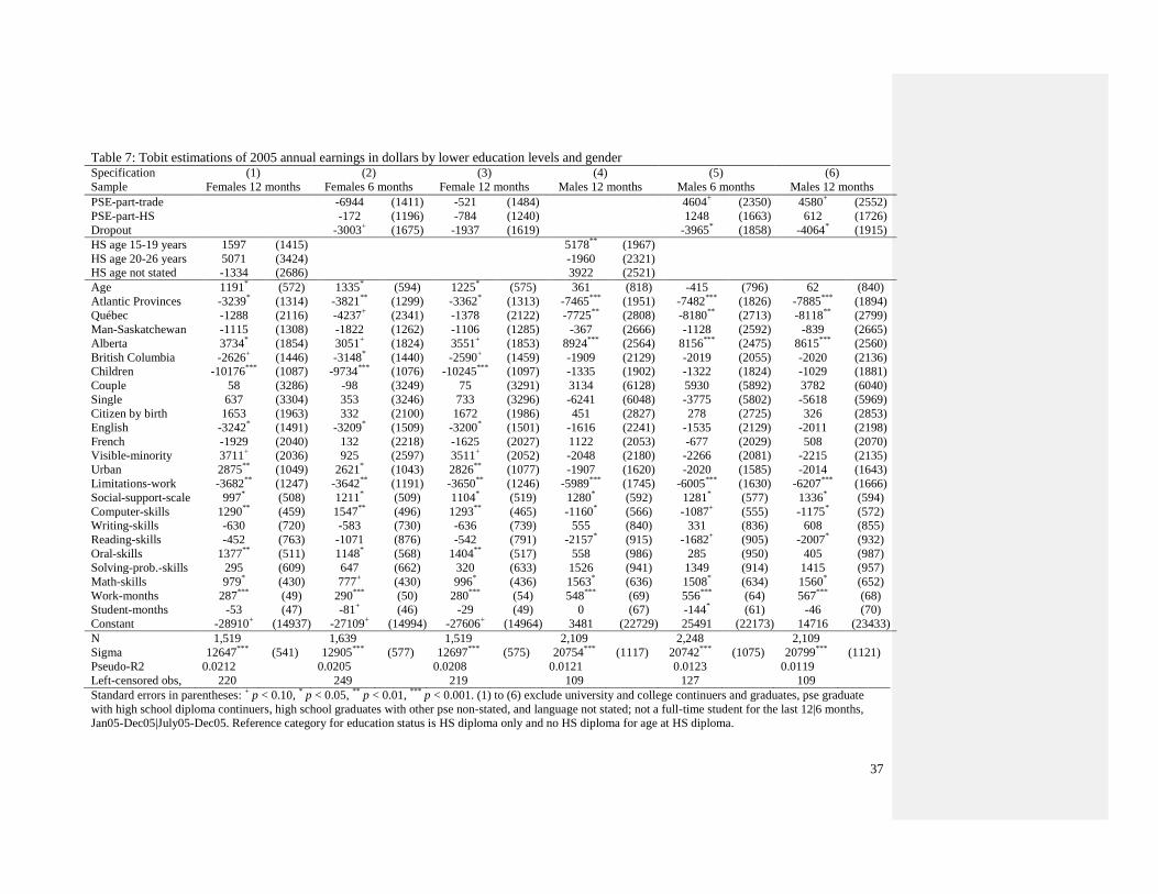
37

Table 7: Tobit estimations of 2005 annual earnings in dollars by lower education levels and gender Specification

Sample

(1)

Females 12 months

(2)

Females 6 months

(3)

Female 12 months

(4)

Males 12 months

(5)

Males 6 months

(6)

Males 12 months

PSE-part-trade -6944 (1411) -521 (1484) 4604+ (2350) 4580

+ (2552)

PSE-part-HS -172 (1196) -784 (1240) 1248 (1663) 612 (1726)

Dropout -3003+ (1675) -1937 (1619) -3965

* (1858) -4064

* (1915)

HS age 15-19 years 1597 (1415) 5178**

(1967)

HS age 20-26 years 5071 (3424) -1960 (2321)

HS age not stated -1334 (2686) 3922 (2521)

Age 1191* (572) 1335

* (594) 1225

* (575) 361 (818) -415 (796) 62 (840)

Atlantic Provinces -3239* (1314) -3821

** (1299) -3362

* (1313) -7465

*** (1951) -7482

*** (1826) -7885

*** (1894)

Québec -1288 (2116) -4237+ (2341) -1378 (2122) -7725

** (2808) -8180

** (2713) -8118

** (2799)

Man-Saskatchewan -1115 (1308) -1822 (1262) -1106 (1285) -367 (2666) -1128 (2592) -839 (2665)

Alberta 3734* (1854) 3051

+ (1824) 3551

+ (1853) 8924

*** (2564) 8156

*** (2475) 8615

*** (2560)

British Columbia -2626+ (1446) -3148

* (1440) -2590

+ (1459) -1909 (2129) -2019 (2055) -2020 (2136)

Children -10176***

(1087) -9734***

(1076) -10245***

(1097) -1335 (1902) -1322 (1824) -1029 (1881)

Couple 58 (3286) -98 (3249) 75 (3291) 3134 (6128) 5930 (5892) 3782 (6040)

Single 637 (3304) 353 (3246) 733 (3296) -6241 (6048) -3775 (5802) -5618 (5969)

Citizen by birth 1653 (1963) 332 (2100) 1672 (1986) 451 (2827) 278 (2725) 326 (2853)

English -3242* (1491) -3209

* (1509) -3200

* (1501) -1616 (2241) -1535 (2129) -2011 (2198)

French -1929 (2040) 132 (2218) -1625 (2027) 1122 (2053) -677 (2029) 508 (2070)

Visible-minority 3711+ (2036) 925 (2597) 3511

+ (2052) -2048 (2180) -2266 (2081) -2215 (2135)

Urban 2875**

(1049) 2621* (1043) 2826

** (1077) -1907 (1620) -2020 (1585) -2014 (1643)

Limitations-work -3682**

(1247) -3642**

(1191) -3650**

(1246) -5989***

(1745) -6005***

(1630) -6207***

(1666)

Social-support-scale 997* (508) 1211

* (509) 1104

* (519) 1280

* (592) 1281

* (577) 1336

* (594)

Computer-skills 1290**

(459) 1547**

(496) 1293**

(465) -1160* (566) -1087

+ (555) -1175

* (572)

Writing-skills -630 (720) -583 (730) -636 (739) 555 (840) 331 (836) 608 (855)

Reading-skills -452 (763) -1071 (876) -542 (791) -2157* (915) -1682

+ (905) -2007

* (932)

Oral-skills 1377**

(511) 1148* (568) 1404

** (517) 558 (986) 285 (950) 405 (987)

Solving-prob.-skills 295 (609) 647 (662) 320 (633) 1526 (941) 1349 (914) 1415 (957)

Math-skills 979* (430) 777

+ (430) 996

* (436) 1563

* (636) 1508

* (634) 1560

* (652)

Work-months 287***

(49) 290***

(50) 280***

(54) 548***

(69) 556***

(64) 567***

(68)

Student-months -53 (47) -81+ (46) -29 (49) 0 (67) -144

* (61) -46 (70)

Constant -28910+ (14937) -27109

+ (14994) -27606

+ (14964) 3481 (22729) 25491 (22173) 14716 (23433)

N

Sigma

Pseudo-R2

Left-censored obs,

1,519

12647***

0.0212

220

(541)

1,639

12905***

0.0205

249

(577)

1,519

12697***

0.0208

219

(575)

2,109

20754***

0.0121

109

(1117)

2,248

20742***

0.0123

127

(1075)

2,109

20799***

0.0119

109

(1121)

Standard errors in parentheses: + p < 0.10,

* p < 0.05,

** p < 0.01,

*** p < 0.001. (1) to (6) exclude university and college continuers and graduates, pse graduate

with high school diploma continuers, high school graduates with other pse non-stated, and language not stated; not a full-time student for the last 12|6 months,

Jan05-Dec05|July05-Dec05. Reference category for education status is HS diploma only and no HS diploma for age at HS diploma.

38

Table 8: OLS estimation of log hourly wage rate by educational levels and gender

Specification

Sample

(1)

Females

(2)

Females

(3)

Females

Lower education

(1)

Males

(2)

Males

(3)

Males

Lower education

College graduate -0.177***

(0.03) -0.189***

(0.03) -0.163***

(0.04) -0.165***

(0.04)

PSE-trade -0.228***

(0.05) -0.239***

(0.05) 0.100+ (0.05) -0.164

** (0.05) -0.167

** (0.06) 0.185

*** (0.05)

PSE-part-HS -0.277***

(0.04) -0.271***

(0.04) 0.071 (0.05) -0.285***

(0.05) -0.286***

(0.05) 0.042 (0.04)

High school-only -0.176***

(0.05) -0.204***

(0.05) 0.133* (0.05) -0.169

** (0.06) -0.182

** (0.06) 0.151

** (0.05)

High-School-other -0.350***

(0.05) -0.345***

(0.05) -0.313***

(0.05) -0.311***

(0.05)

Dropout -0.307***

(0.06) -0.308***

(0.06) 0.038 (0.05) -0.393***

(0.06) -0.390***

(0.06) -0.079* (0.04)

Age 0.060***

(0.01) 0.053***

(0.01) 0.048* (0.02) 0.039

** (0.01) 0.037

** (0.01) 0.027 (0.02)

Atlantic Provinces -0.159***

(0.03) -0.165***

(0.03) -0.220***

(0.04) -0.198***

(0.03) -0.200***

(0.03) -0.225***

(0.04)

Québec 0.022 (0.05) -0.011 (0.04) -0.094 (0.07) -0.079+ (0.04) -0.075 (0.05) -0.172

*** (0.05)

Man-Saskatchewan -0.105**

(0.03) -0.122***

(0.03) -0.114* (0.05) -0.116

*** (0.03) -0.126

*** (0.04) -0.189

*** (0.05)

Alberta 0.052 (0.04) 0.057 (0.04) 0.055 (0.06) 0.097**

(0.03) 0.098**

(0.03) 0.058 (0.04)

British Columbia 0.007 (0.04) -0.008 (0.03) -0.020 (0.05) 0.049 (0.04) 0.036 (0.04) 0.009 (0.06)

Children -0.117***

(0.03) -0.114***

(0.03) -0.085* (0.03) 0.047 (0.03) 0.050 (0.03) 0.015 (0.04)

Couple -0.008 (0.08) 0.003 (0.08) 0.034 (0.09) 0.017 (0.08) -0.003 (0.08) 0.018 (0.09)

Single -0.093 (0.08) -0.081 (0.08) -0.004 (0.09) -0.077 (0.08) -0.098 (0.08) -0.088 (0.09)

Citizen by birth -0.004 (0.05) 0.001 (0.05) 0.078 (0.10) -0.005 (0.05) -0.020 (0.05) -0.035 (0.07)

English 0.034 (0.04) 0.017 (0.03) -0.075+ (0.04) -0.051 (0.04) -0.047 (0.04) -0.088

* (0.04)

French -0.003 (0.04) 0.018 (0.04) 0.038 (0.07) 0.016 (0.04) 0.013 (0.04) 0.065 (0.05)

Visible-minority -0.012 (0.05) -0.015 (0.05) -0.011 (0.08) -0.049 (0.04) -0.079 (0.05) -0.114* (0.06)

Urban 0.019 (0.03) 0.022 (0.03) 0.094* (0.04) 0.020 (0.02) 0.027 (0.03) 0.028 (0.03)

Limitations-work -0.061* (0.02) -0.054

* (0.03) -0.059

+ (0.03) -0.009 (0.03) -0.010 (0.03) -0.003 (0.03)

Social-support-scale 0.026* (0.01) 0.026

* (0.01) 0.014 (0.02) 0.011 (0.01) 0.009 (0.01) 0.036

** (0.01)

Computer-skill 0.019 (0.01) 0.023+ (0.01) 0.028 (0.02) -0.006 (0.01) -0.005 (0.01) -0.015 (0.01)

Writing-skill -0.007 (0.02) -0.010 (0.02) -0.017 (0.02) 0.005 (0.01) 0.011 (0.02) 0.015 (0.02)

Reading-skill 0.002 (0.02) 0.004 (0.02) 0.033 (0.02) -0.040**

(0.01) -0.035* (0.02) -0.019 (0.02)

Oral-skill 0.015 (0.01) 0.015 (0.01) 0.003 (0.02) -0.023+ (0.01) -0.021 (0.01) -0.003 (0.02)

Solving-prob.-skill 0.005 (0.02) 0.004 (0.02) -0.008 (0.03) 0.036* (0.02) 0.030

+ (0.02) -0.003 (0.02)

Math-skill 0.030**

(0.01) 0.029**

(0.01) 0.034* (0.01) 0.040

*** (0.01) 0.037

** (0.01) 0.036

** (0.01)

Work-months 0.001 (0.00) 0.001 (0.00) 0.002 (0.00) 0.007***

(0.00) 0.007***

(0.00) 0.009***

(0.00)

Student-months 0.002+ (0.00) 0.003

* (0.00) 0.002 (0.00) -0.000 (0.00) 0.001 (0.00) -0.001 (0.00)

Constant 1.054**

(0.39) 1.233**

(0.38) 0.826 (0.53) 1.820***

(0.37) 1.844***

(0.39) 1.853***

(0.45)

N 4,029 3,609 1,539 4,006 3,663 2,116

Adj. R2 0.187 0.204 0.109 0.147 0.158 0.149

Marginal effects; for discrete change of dummy variable from 0 to 1; Standard errors in parentheses: + p < 0.10, * p < 0.05, ** p < 0.01, *** p < 0.001.

(1) to (3) exclude university and college continuers, pse graduate with high school continuers, and language not stated; (3) also excludes university and college graduates;

(2) not a full-time student for the last 6 months, July05-Dec05; (3) not a full-time student for the last 12 months, Jan05-Dec05. Reference category for education status is

university graduate (1) and (2); High-School-other (3).

39

Table 9: OLS estimation of ln hourly wage rate by lower educational levels and gender

Specification (1) (2) (3) (1) (2) (3)

Sample Females Females Females Males Males Males

PSE-trade 0.12* (0.05) 0.10

+ (0.05) 0.19

*** (0.05) 0.18

*** (0.05)

PSE-part-HS 0.08+ (0.05) 0.07 (0.05) 0.05 (0.04) 0.04 (0.04)

Dropout 0.05 (0.05) 0.04 (0.05) -0.08* (0.04) -0.08

* (0.04)

HS age 15-19 years -0.01 (0.05) 0.07+ (0.04)

HS age 20-26 years 0.05 (0.10) 0.06 (0.05)

HS age not stated 0.03 (0.08) 0.07 (0.06)

Age 0.04* (0.02) 0.05

* (0.02) 0.06

** (0.02) 0.01 (0.02) 0.03 (0.02) 0.04

* (0.02)

Atlantic provinces -0.22***

(0.04) -0.22***

(0.04) -0.2***

(0.04) -0.20***

(0.04) -0.21***

(0.05) -0.2***

(0.05)

Québec -0.03 (0.07) -0.06 (0.08) -0.05 (0.08) -0.16**

(0.05) -0.16**

(0.05) -0.2**

(0.05)

Man-Saskatchewan -0.15**

(0.05) -0.13* (0.05) -0.1

* (0.06) -0.19

*** (0.05) -0.19

*** (0.05) -0.2

*** (0.05)

Alberta 0.03 (0.06) 0.04 (0.06) 0.03 (0.06) 0.06 (0.04) 0.07 (0.04) 0.07+ (0.04)

British Columbia -0.06 (0.05) -0.04 (0.05) -0.05 (0.05) 0.01 (0.06) 0.02 (0.06) 0.03 (0.06)

Children -0.10**

(0.03) -0.09**

(0.04) -0.09* (0.04) 0.00 (0.04) 0.02 (0.04) 0.01 (0.04)

Couple 0.00 (0.10) 0.01 (0.10) -0.001 (0.10) 0.03 (0.10) 0.03 (0.10) 0.02 (0.10)

Single -0.04 (0.10) -0.01 (0.10) -0.02 (0.10) -0.08 (0.10) -0.07 (0.10) -0.08 (0.10)

Citizen by birth 0.18+ (0.10) 0.15 (0.11) 0.2 (0.11) -0.04 (0.06) -0.03 (0.07) -0.01 (0.07)

English -0.05 (0.05) -0.07 (0.05) -0.07 (0.05) -0.08* (0.04) -0.08

* (0.04) -0.08

+ (0.04)

French -0.05 (0.07) -0.02 (0.07) -0.04 (0.08) 0.04 (0.05) 0.07 (0.05) 0.06 (0.05)

Visible minority 0.04 (0.07) 0.02 (0.08) 0.01 (0.08) -0.09+ (0.05) -0.11

+ (0.06) -0.1

+ (0.06)

Urban 0.09* (0.04) 0.09

* (0.04) 0.10

* (0.04) 0.03 (0.03) 0.03 (0.03) 0.03 (0.03)

Limitations-work -0.05 (0.03) -0.06+ (0.03) -0.06

+ (0.03) 0.00 (0.03) 0.001 (0.03) -0.00 (0.04)

Social-support-scale 0.03+ (0.02) 0.03

+ (0.02) 0.04

* (0.02) 0.04

** (0.01) 0.04

** (0.01) 0.04

** (0.01)

Computer-skill 0.01 (0.02) 0.02 (0.02) 0.02 (0.02) -0.01 (0.01) -0.01 (0.01) -0.006 (0.01)

Writing-skill -0.02 (0.02) -0.01 (0.02) -0.01 (0.02) 0.01 (0.02) 0.02 (0.02) 0.02 (0.02)

Reading-skill 0.04 (0.03) 0.04 (0.03) 0.04 (0.03) -0.03 (0.02) -0.02 (0.02) -0.03+ (0.02)

Oral-skill 0.01 (0.02) 0.00 (0.02) -0.001 (0.02) -0.01 (0.02) -0.01 (0.02) -0.008 (0.02)

Solving-prob.-skill -0.02 (0.03) -0.01 (0.03) -0.01 (0.03) 0.002 (0.02) -0.00 (0.02) -0.00 (0.02)

Math-skill 0.03+ (0.01) 0.03

+ (0.02) 0.03

+ (0.02) 0.04

** (0.01) 0.04

** (0.01) 0.04

* (0.01)

Work-months 0.002 (0.00) 0.00 (0.00) 0.002 (0.00) 0.01***

(0.00) 0.01***

(0.00) 0.01***

(0.00)

Student-months 0.00 (0.00) 0.00 (0.00) 0.003+ (0.00) -0.00 (0.00) -0.00 (0.00) 0.00 (0.00)

Constant 1.00+ (0.56) 0.8 (0.59) 0.6 (0.57) 2.17

*** (0.44) 1.82

*** (0.47) 1.4

** (0.46)

N 1,445 1,342 1,342 2,082 1,957 1,957 1,957

Adjusted R2 0.116 0.114 0.111 0.158 0.161 0.148 0.148

Standard errors in parentheses: + p < 0.10,

* p < 0.05,

** p < 0.01,

*** p < 0.001. (1) to (3) exclude university and college graduates and continuers, pse graduate

with high school continuers, high school graduates with other non-stated pse, and language not stated; (1) not a full-time student for the last 6 months, July05-

Dec05; (2) and (3) non a full-time student for the last12 months, Jan05-Dec05. Reference is High-School-other and dropout for age at high school diploma.

40

Table 10: OLS estimations of monthly earnings when last worked at job by educational levels and gender

Specification (1) (2) (3) (1) (2) (3)

Sample Females

6 months

Females

12 months

Females lower

education 12 months

Males

6 months

Males

12 months

Male lower

education 12 months

College graduate -461***

(89) -485***

(95) -383**

(121) -428**

(134)

PSE-trade -637***

(137) -634***

(141) 134 (129) -276 (198) -363+ (214) 599

*** (181)

PSE-part-HS -664***

(114) -657***

(119) 96 (104) -622***

(132) -670***

(147) 256* (128)

High-School-other -786***

(140) -779***

(146) -788***

(151) -830***

(165)

Dropout -813***

(153) -820***

(159) -53 (117) -924***

(184) -974***

(194) -141 (120)

Age 113**

(37) 89* (37) 39 (53) 67 (45) 50 (47) 15 (57)

Atlantic Provinces -268***

(73) -274***

(75) -348***

(89) -395***

(105) -380***

(114) -334* (149)

Québec -32 (111) -34 (107) -321+ (181) -333

** (113) -307

* (119) -507

** (156)

Man-Saskatchewan -169* (83) -208

* (87) -164 (111) -239

* (103) -272

* (107) -346

* (140)

Alberta 159 (113) 168 (119) 194 (171) 574***

(123) 586***

(131) 526**

(161)

British Columbia -227* (100) -266

** (99) -264

* (118) 14 (135) -33 (146) -31 (167)

Children -332***

(68) -331***

(70) -271***

(78) 73 (120) 105 (124) 46 (144)

Couple -344 (247) -332 (255) -216 (206) -21 (355) -115 (369) -51 (384)

Single -503* (251) -483

+ (259) -328 (206) -331 (352) -413 (365) -356 (378)

Citizen by birth -163 (136) -147 (144) -3 (215) -139 (122) -194 (125) -241 (167)

English 38 (88) 31 (84) -253* (116) -96 (94) -62 (100) -118 (130)

French -74 (91) -79 (91) 102 (162) 49 (129) 106 (124) 204 (136)

Visible-minority 111 (136) 106 (143) 73 (209) -195 (120) -205 (127) -447**

(151)

Urban 93 (64) 90 (66) 135 (91) -63 (89) -43 (93) -20 (114)

Limitations-work -195**

(68) -184**

(70) -211* (83) -124 (110) -141 (115) 101 (131)

Social-support-scale 55+ (31) 51 (32) 44 (42) 60

+ (34) 66

+ (35) 122

** (44)

Computer-skill 66* (31) 77

* (32) 130

** (40) -64

+ (37) -81

* (38) -130

** (44)

Writing-skill 5 (45) 0 (47) 7 (48) -11 (52) 14 (55) -3 (65)

Reading-skill -15 (48) -5 (50) 24 (64) -102+ (53) -99

+ (56) -36 (61)

Oral-skill 68* (33) 78

* (35) 24 (41) -59 (50) -48 (53) -57 (65)

Solving-prob.-skill -1 (43) -9 (45) -31 (65) 75+ (46) 82

+ (48) 18 (57)

Math-skill 89***

(25) 78**

(26) 52 (34) 166***

(37) 129***

(38) 117**

(45)

Work-months 0 (3) 2 (3) 4 (6) 13***

(3) 14***

(3) 17***

(4)

Student-months 0 (3) 2 (3) 3 (4) -4 (3) 0 (3) -4 (5)

Constant -433 (1054) 56 (1061) 417 (1469) 1698 (1244) 2209+ (1326) 2490 (1557)

N 3,764

0.169

3,369

0.184

1,327

0.115

3,808

0.107

3,478

0.111

1,943

0.117 Adjusted-R2

Standard errors in parentheses: + p < 0.10,

* p < 0.05,

** p < 0.01,

*** p < 0.001. (1) to (3) exclude university and college continuers, pse graduate with high school

continuers, high school graduate with other non-stated pse, and language not stated; (1) not a full-time student for the last 6 months, July05-Dec05; (2) and (3) not

a full-time student for the last 12 months, Jan05-Dec05. Reference category for education status is university graduate and HS diploma for lower education

samples.

41

Table 11: Marginal effects of Probit estimations of employer or career or total training by level of education and gender

Specification (1) (2) (3) (4) (5) (6)

Sample Female Employer Male Employer Female Career Male Career Female both training Male both training

College graduate -0.045 (0.04) 0.009 (0.04) -0.026 (0.02) -0.006 (0.03) -0.074+ (0.04) -0.019 (0.05)

PSE-trade -0.111**

(0.06) -0.006 (0.07) -0.048**

(0.02) -0.072****

(0.02) -0.135**

(0.06) -0.075 (0.07)

PSE-part-HS -0.093+ (0.05) 0.021 (0.05) -0.050

** (0.02) -0.013 (0.03) -0.101

+ (0.05) 0.005 (0.05)

High-School-other -0.164***

(0.06) -0.010 (0.06) -0.062**

(0.03) -0.019 (0.03) -0.186***

(0.06) -0.044 (0.06)

Dropout -0.121+ (0.07) -0.035 (0.07) -0.066

** (0.03) -0.024 (0.04) -0.188

*** (0.07) -0.072 (0.07)

Age 0.012 (0.02) -0.004 (0.02) 0.002 (0.01) 0.012 (0.01) 0.010 (0.02) 0.003 (0.02)

Atlantic Provinces 0.001 (0.04) -0.005 (0.04) -0.032+ (0.02) -0.043

*** (0.02) -0.017 (0.04) -0.026 (0.04)

Québec -0.131***

(0.05) -0.086+ (0.05) 0.006 (0.03) -0.074

**** (0.02) -0.096

+ (0.05) -0.127

*** (0.05)

Man-Saskatchewan 0.003 (0.04) 0.089**

(0.04) -0.008 (0.02) 0.003 (0.02) 0.004 (0.04) 0.093**

(0.04)

Alberta -0.009 (0.04) 0.068 (0.04) 0.035 (0.03) 0.083**

(0.04) 0.005 (0.04) 0.127***

(0.04)

British Columbia 0.028 (0.05) 0.015 (0.05) 0.086***

(0.03) -0.000 (0.03) 0.085+ (0.05) 0.014 (0.05)

Children -0.071**

(0.04) -0.008 (0.04) -0.032+ (0.02) -0.002 (0.02) -0.081

** (0.04) 0.003 (0.04)

Couple 0.084 (0.08) -0.058 (0.11) 0.196**

(0.08) -0.054 (0.05) 0.147+ (0.08) -0.091 (0.12)

Single 0.054 (0.09) -0.150 (0.12) 0.194**

(0.08) -0.047 (0.06) 0.132 (0.09) -0.174 (0.12)

Citizen by birth -0.053 (0.06) 0.019 (0.06) 0.007 (0.03) 0.005 (0.03) -0.009 (0.06) 0.038 (0.06)

English -0.041 (0.04) -0.039 (0.04) 0.005 (0.02) -0.044+ (0.02) -0.022 (0.04) -0.068

+ (0.04)

French 0.045 (0.05) -0.014 (0.05) -0.019 (0.03) 0.001 (0.03) 0.043 (0.05) 0.002 (0.05)

Visible-minority 0.003 (0.06) -0.102+ (0.05) -0.010 (0.03) -0.048

** (0.02) 0.002 (0.06) -0.110

+ (0.06)

Urban 0.009 (0.03) 0.037 (0.03) -0.012 (0.02) -0.047**

(0.02) 0.022 (0.03) 0.026 (0.03)

Limitations-work 0.003 (0.04) -0.012 (0.04) 0.044**

(0.02) -0.021 (0.02) 0.044 (0.04) -0.011 (0.04)

Social-support-scale 0.022 (0.02) 0.056****

(0.01) 0.001 (0.01) 0.012 (0.01) 0.036**

(0.02) 0.048****

(0.01)

Computer-skill -0.023 (0.01) -0.015 (0.01) -0.010 (0.01) 0.016+ (0.01) -0.022 (0.01) -0.010 (0.01)

Writing-skill -0.011 (0.02) 0.013 (0.02) 0.004 (0.02) -0.005 (0.01) -0.019 (0.02) 0.024 (0.02)

Reading-skill 0.017 (0.02) -0.043**

(0.02) -0.013 (0.01) -0.014 (0.01) 0.008 (0.02) -0.047**

(0.02)

Oral-skill 0.022 (0.02) 0.025 (0.02) 0.004 (0.01) 0.017+ (0.01) 0.016 (0.02) 0.042

** (0.02)

Solving-prob.-skill 0.062***

(0.02) 0.037**

(0.02) 0.017 (0.01) -0.004 (0.01) 0.072****

(0.02) 0.025 (0.02)

Math-skill -0.006 (0.01) -0.018 (0.01) 0.001 (0.01) 0.010 (0.01) -0.006 (0.01) -0.009 (0.01)

Work-months 0.002 (0.00) 0.003**

(0.00) 0.000 (0.00) -0.001 (0.00) 0.001 (0.00) 0.003**

(0.00)

Student-months 0.001 (0.00) 0.002**

(0.00) 0.000 (0.00) 0.000 (0.00) 0.000 (0.00) 0.003**

(0.00)

N 3,527 3,643 3,708 3,736 3,527 3,643

Pseudo-R2 0.0454 0.0443 0.0460 0.0516 0.0481 0.0519

Marginal effects for discrete change of dummy variable from 0 to 1; Standard errors in parentheses: + p < 0.10,

** p < 0.05,

*** p < 0.01,

**** p < 0.001.

(1) to (6) excludes university and college continuers, pse graduate with high school continuers, high school graduates with other non-stated pse, and language not

stated; not a full-time student for the last 12 months, Jan05-Dec05. Reference category for education status is university graduate.

42

Table 12: Marginal effects of Probit estimations of employer or career or total training by lower level of education and gender

Specification (1) (2) (3) (4) (5) (6)

Sample Female Employer Male employer Female career Male career Female all Male all

PSE-trade 0.055 (0.06) -0.009 (0.07) -0.001 (0.03) -0.064****

(0.02) 0.044 (0.06) -0.059 (0.07)

PSE-part-HS 0.069 (0.05) 0.025 (0.04) 0.003 (0.02) -0.003 (0.02) 0.074 (0.05) 0.036 (0.04)

Dropout 0.021 (0.06) -0.014 (0.05) -0.008 (0.03) -0.007 (0.03) -0.019 (0.06) -0.016 (0.05)

Age 0.002 (0.03) -0.011 (0.02) 0.008 (0.01) 0.017 (0.01) 0.004 (0.03) 0.009 (0.02)

Atlantic Provinces -0.001 (0.06) -0.014 (0.05) -0.010 (0.02) -0.034+ (0.02) -0.016 (0.06) -0.014 (0.05)

Québec -0.107 (0.08) -0.111+ (0.07) 0.160

** (0.08) -0.103

**** (0.02) -0.011 (0.09) -0.169

** (0.07)

Man-Saskatchewan 0.100 (0.06) 0.027 (0.05) 0.029 (0.04) 0.013 (0.03) 0.100 (0.06) 0.044 (0.05)

Alberta 0.043 (0.06) 0.023 (0.05) 0.043 (0.04) 0.065 (0.04) 0.073 (0.07) 0.101+ (0.06)

British Columbia 0.056 (0.07) 0.059 (0.06) 0.112**

(0.05) 0.040 (0.04) 0.145**

(0.07) 0.088 (0.07)

Children 0.030 (0.05) -0.072 (0.05) -0.031 (0.02) -0.011 (0.02) 0.011 (0.05) -0.068 (0.05)

Couple 0.129 (0.10) -0.043 (0.13) 0.089 (0.06) -0.047 (0.04) 0.192+ (0.10) -0.072 (0.13)

Single 0.206**

(0.10) -0.129 (0.13) 0.134+ (0.07) -0.056 (0.06) 0.301

*** (0.10) -0.168 (0.13)

Citizen by birth 0.080 (0.09) 0.078 (0.07) 0.020 (0.03) 0.044**

(0.02) 0.077 (0.10) 0.110 (0.07)

English -0.050 (0.06) -0.013 (0.05) 0.049**

(0.02) -0.102***

(0.03) -0.016 (0.06) -0.070 (0.06)

French 0.151+ (0.09) -0.007 (0.06) -0.053

** (0.02) 0.023 (0.04) 0.073 (0.09) 0.015 (0.07)

Visible-minority 0.106 (0.12) -0.133**

(0.07) -0.032 (0.03) -0.048**

(0.02) 0.068 (0.11) -0.143**

(0.07)

Urban 0.031 (0.05) 0.032 (0.03) -0.016 (0.03) -0.037+ (0.02) 0.011 (0.05) 0.035 (0.04)

Limitations-work -0.011 (0.04) 0.014 (0.04) 0.020 (0.02) -0.022 (0.02) 0.031 (0.05) 0.007 (0.04)

Social-support-scale 0.006 (0.02) 0.060****

(0.02) 0.015 (0.01) 0.004 (0.01) 0.022 (0.02) 0.048***

(0.02)

Computer-skill 0.002 (0.02) -0.016 (0.02) -0.013 (0.01) 0.013 (0.01) 0.002 (0.02) -0.011 (0.02)

Writing-skill 0.004 (0.03) 0.023 (0.02) -0.002 (0.02) -0.015 (0.01) -0.018 (0.03) 0.034 (0.03)

Reading-skill 0.041 (0.03) -0.054**

(0.02) -0.002 (0.02) -0.008 (0.01) 0.052 (0.03) -0.062**

(0.03)

Oral-skill 0.020 (0.02) 0.029 (0.02) 0.002 (0.01) 0.011 (0.01) 0.019 (0.03) 0.046**

(0.02)

Solving-prob.-skill 0.020 (0.03) 0.062***

(0.02) 0.019 (0.01) 0.004 (0.01) 0.030 (0.03) 0.043+ (0.02)

Math-skill 0.010 (0.02) -0.018 (0.02) -0.003 (0.01) 0.011 (0.01) 0.002 (0.02) -0.001 (0.02)

Work-months 0.003+ (0.00) 0.004

** (0.00) 0.000 (0.00) -0.001 (0.00) 0.003 (0.00) 0.003

+ (0.00)

Student-months 0.000 (0.00) 0.003 (0.00) 0.001 (0.00) 0.001 (0.00) 0.001 (0.00) 0.004**

(0.00)

N 1,383 2,043 1,518 2,109 1,383 2,043

Pseudo-R2 0.048 0.0614 0.0839 0.0800 0.0583 0.0678

Marginal effects for discrete change of dummy variable from 0 to 1; Standard errors in parentheses: + p < 0.10,

** p < 0.05,

*** p < 0.01,

**** p < 0.001.

(1) to (6) excludes university and college continuers, pse graduate with high school continuers, high school graduates with other not-stated pse, language not

stated; not a full-time student for the last 12 months (Jan05-Dec05). Reference category for education status is high school diploma only.

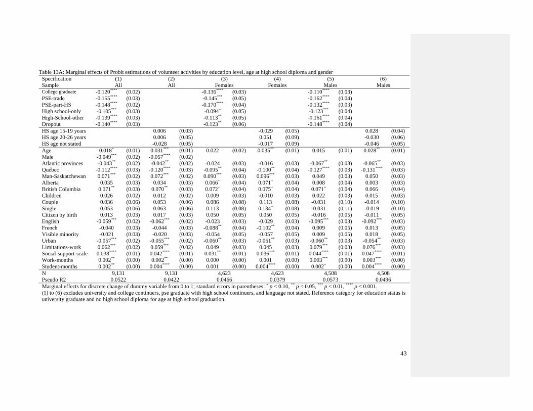
43

Table 13A: Marginal effects of Probit estimations of volunteer activities by education level, age at high school diploma and gender

Specification (1) (2) (3) (4) (5) (6)

Sample All All Females Females Males Males College graduate -0.120

**** (0.02) -0.136

**** (0.03) -0.110

**** (0.03)

PSE-trade -0.155****

(0.03) -0.145***

(0.05) -0.162****

(0.04)

PSE-part-HS -0.148****

(0.02) -0.170****

(0.04) -0.132****

(0.03)

High school-only -0.105***

(0.03) -0.094+ (0.05) -0.123

*** (0.04)

High-School-other -0.139****

(0.03) -0.113**

(0.05) -0.161****

(0.04)

Dropout -0.140****

(0.03) -0.123**

(0.06) -0.148****

(0.04)

HS age 15-19 years 0.006 (0.03) -0.029 (0.05) 0.028 (0.04)

HS age 20-26 years 0.006 (0.05) 0.051 (0.09) -0.030 (0.06)

HS age not stated -0.028 (0.05) -0.017 (0.09) -0.046 (0.05)

Age 0.018+ (0.01) 0.031

*** (0.01) 0.022 (0.02) 0.035

** (0.01) 0.015 (0.01) 0.028

** (0.01)

Male -0.049***

(0.02) -0.057****

(0.02)

Atlantic provinces -0.043**

(0.02) -0.042**

(0.02) -0.024 (0.03) -0.016 (0.03) -0.067**

(0.03) -0.065**

(0.03)

Québec -0.112****

(0.03) -0.120****

(0.03) -0.095**

(0.04) -0.100**

(0.04) -0.127****

(0.03) -0.131****

(0.03)

Man-Saskatchewan 0.071***

(0.02) 0.072***

(0.02) 0.090***

(0.03) 0.096***

(0.03) 0.049 (0.03) 0.050 (0.03)

Alberta 0.035 (0.03) 0.034 (0.03) 0.066+ (0.04) 0.071

+ (0.04) 0.008 (0.04) 0.003 (0.03)

British Columbia 0.071**

(0.03) 0.070**

(0.03) 0.072+ (0.04) 0.075

+ (0.04) 0.071

+ (0.04) 0.066 (0.04)

Children 0.026 (0.02) 0.012 (0.02) 0.009 (0.03) -0.010 (0.03) 0.022 (0.03) 0.015 (0.03)

Couple 0.036 (0.06) 0.053 (0.06) 0.086 (0.08) 0.113 (0.08) -0.031 (0.10) -0.014 (0.10)

Single 0.053 (0.06) 0.063 (0.06) 0.113 (0.08) 0.134+ (0.08) -0.031 (0.11) -0.019 (0.10)

Citizen by birth 0.013 (0.03) 0.017 (0.03) 0.050 (0.05) 0.050 (0.05) -0.016 (0.05) -0.011 (0.05)

English -0.059***

(0.02) -0.062***

(0.02) -0.023 (0.03) -0.029 (0.03) -0.095***

(0.03) -0.092***

(0.03)

French -0.040 (0.03) -0.044 (0.03) -0.088**

(0.04) -0.102**

(0.04) 0.009 (0.05) 0.013 (0.05)

Visible minority -0.021 (0.03) -0.020 (0.03) -0.054 (0.05) -0.057 (0.05) 0.009 (0.05) 0.018 (0.05)

Urban -0.057***

(0.02) -0.055***

(0.02) -0.060**

(0.03) -0.061**

(0.03) -0.060**

(0.03) -0.054**

(0.03)

Limitations-work 0.062***

(0.02) 0.059***

(0.02) 0.049 (0.03) 0.045 (0.03) 0.079***

(0.03) 0.076***

(0.03)

Social-support-scale 0.038****

(0.01) 0.042****

(0.01) 0.031**

(0.01) 0.036***

(0.01) 0.044****

(0.01) 0.047****

(0.01)

Work-months 0.002**

(0.00) 0.002**

(0.00) 0.000 (0.00) 0.001 (0.00) 0.003***

(0.00) 0.003***

(0.00)

Student-months 0.002**

(0.00) 0.004****

(0.00) 0.001 (0.00) 0.004****

(0.00) 0.002+ (0.00) 0.004

**** (0.00)

N

Pseudo R2

9,131

0.0522

9,131

0.0422

4,623

0.0466

4,623

0.0379

4,508

0.0573

4,508

0.0496

Marginal effects for discrete change of dummy variable from 0 to 1; standard errors in parentheses: + p < 0.10,

** p < 0.05,

*** p < 0.01,

**** p < 0.001.

(1) to (6) excludes university and college continuers, pse graduate with high school continuers, and language not stated. Reference category for education status is

university graduate and no high school diploma for age at high school graduation.

44

Table 13B: Marginal effects of Probit estimations of volunteer activities by lower education level, age at high school diploma and gender

Specification (1) (2) (3) (4) (5) (6)

Sample All All Females Females Males Males

PSE-trade -0.050 (0.04) -0.070 (0.05) -0.037 (0.05)

PSE-part-HS -0.039 (0.03) -0.084+ (0.04) -0.002 (0.03)

High school-only -0.017 (0.04) -0.027 (0.06) -0.008 (0.05)

High-School-other

Dropout 0.020 (0.01) 0.023 (0.02) 0.020 (0.02)

HS age 15-19 years -0.013 (0.05) 0.075 (0.09) -0.080+ (0.05)

HS age 20-26 years 0.022 (0.05) 0.093 (0.10) -0.031 (0.05)

HS age not stated 0.017 (0.01) 0.019 (0.02) 0.018 (0.02)

Male -0.081****

(0.02) -0.078****

(0.02)

Atlantic provinces -0.038 (0.03) -0.039 (0.03) -0.019 (0.05) -0.013 (0.05) -0.060**

(0.03) -0.059+ (0.03)

Québec -0.117***

(0.04) -0.117***

(0.04) -0.198****

(0.06) -0.195***

(0.06) -0.072 (0.05) -0.062 (0.05)

Man-Saskatchewan 0.070**

(0.03) 0.071**

(0.03) 0.053 (0.05) 0.059 (0.05) 0.083+ (0.04) 0.084

** (0.04)

Alberta 0.030 (0.04) 0.032 (0.04) 0.036 (0.06) 0.041 (0.06) 0.027 (0.04) 0.026 (0.04)

British Columbia 0.027 (0.04) 0.027 (0.04) 0.005 (0.06) 0.009 (0.06) 0.038 (0.05) 0.033 (0.05)

Children -0.002 (0.03) -0.001 (0.03) 0.004 (0.04) -0.000 (0.04) -0.022 (0.04) -0.022 (0.04)

Couple 0.028 (0.07) 0.027 (0.07) 0.077 (0.09) 0.087 (0.09) -0.025 (0.10) -0.028 (0.10)

Single 0.039 (0.07) 0.038 (0.07) 0.109 (0.09) 0.118 (0.09) -0.038 (0.11) -0.039 (0.11)

Citizen by birth -0.021 (0.05) -0.025 (0.05) -0.005 (0.08) -0.009 (0.08) -0.025 (0.07) -0.034 (0.07)

English -0.064+ (0.03) -0.064

+ (0.03) -0.038 (0.05) -0.037 (0.05) -0.078

+ (0.04) -0.075

+ (0.04)

French -0.047 (0.04) -0.041 (0.04) -0.029 (0.07) -0.034 (0.07) -0.034 (0.05) -0.028 (0.05)

Visible minority -0.015 (0.05) -0.016 (0.05) -0.107 (0.07) -0.106 (0.07) 0.065 (0.07) 0.070 (0.07)

Urban -0.048+ (0.03) -0.051

** (0.03) -0.017 (0.04) -0.022 (0.04) -0.070

** (0.03) -0.070

** (0.03)

Limitations-work 0.038+ (0.02) 0.039

+ (0.02) 0.014 (0.04) 0.017 (0.03) 0.057

** (0.03) 0.061

** (0.03)

Social-support-scale 0.033***

(0.01) 0.032***

(0.01) 0.013 (0.02) 0.015 (0.02) 0.046****

(0.01) 0.044****

(0.01)

Work-months 0.001 (0.00) 0.001 (0.00) 0.000 (0.00) 0.000 (0.00) 0.002 (0.00) 0.002 (0.00)

Student-months 0.003***

(0.00) 0.003***

(0.00) 0.003**

(0.00) 0.002+ (0.00) 0.003

*** (0.00) 0.003

*** (0.00)

N

Pseudo R2

4,394

0.0348

4,394

0.0336

1,920

0.0393

1,920

0.0400

2,474

0.0387

2,474

0.0414

Marginal effects for discrete change of dummy variable from 0 to 1; standard errors in parentheses: + p < 0.10,

** p < 0.05,

*** p < 0.01,

**** p < 0.001.

(1) to (6) excludes university and college graduates and continuers, PSE graduate with high school continuers, and language not stated. Reference category for

education status is high diploma only and no high school diploma for age at high school graduation.

45

Table 14: Odds ratio of ordered logit of frequency of volunteer activities by education levels and gender Specification (1) (2) (3) (4) (5) (6) (7) (8)

Sample Females Females Males Males Females Females Males Males

Lower education

College graduate -0.585**** -0.541****

(0.14) (0.16)

PSE-trade -0.689*** -0.918*** -0.318 -0.175

(0.24) (0.32) (0.28) (0.31)

PSE-part-HS -0.753**** -0.724**** -0.319 -0.044

(0.21) (0.19) (0.22) (0.20)

High school-only -0.411+ -0.631** -0.084 -0.003

(0.24) (0.25) (0.28) (0.30)

High-School-other -0.583** -0.872****

(0.24) (0.23)

Dropout -0.567** -0.865*** 0.0596 0.057

(0.28) (0.29) (0.26) (0.22)

HS age 15-19 years -0.154 0.153 -0.217 0.042

(0.23) (0.20) (0.23) (0.22)

HS age 20-26 years 0.171 -0.221 0.332 -0.606+

(0.36) (0.30) (0.40) (0.35)

HS age not stated -0.068 -0.300 0.415 -0.230

(0.42) (0.30) (0.47) (0.32)

Age 0.083 0.146** 0.072 0.141** 0.129 0.113 0.140 0.133

(0.06) (0.06) (0.07) (0.07) (0.10) (0.10) (0.10) (0.10)

Atlantic provinces -0.048 -0.015 -0.265+ -0.260+ -0.055 -0.022 -0.389+ -0.382+

(0.14) (0.14) (0.15) (0.15) (0.23) (0.23) (0.21) (0.21)

Québec -0.479*** -0.503*** -0.676**** -0.696**** -1.068*** -1.042*** -0.448 -0.393

(0.17) (0.17) (0.18) (0.18) (0.33) (0.33) (0.28) (0.28)

Man-Saskatchewan 0.390*** 0.413*** 0.320** 0.324** 0.263 0.291 0.480** 0.494**

(0.13) (0.13) (0.15) (0.15) (0.21) (0.21) (0.22) (0.21)

Alberta 0.217 0.233+ 0.0545 0.0340 0.0810 0.101 0.131 0.129

(0.14) (0.14) (0.17) (0.17) (0.22) (0.23) (0.25) (0.25)

British Columbia 0.368** 0.374** 0.382** 0.364+ 0.113 0.129 0.173 0.147

(0.17) (0.17) (0.19) (0.19) (0.27) (0.28) (0.26) (0.26)

Children 0.112 0.024 0.115 0.086 0.090 0.0572 -0.123 -0.124

(0.13) (0.13) (0.16) (0.17) (0.19) (0.19) (0.22) (0.22)

Couple 0.402 0.489 -0.253 -0.234 0.403 0.416 -0.396 -0.402

(0.36) (0.37) (0.60) (0.59) (0.50) (0.49) (0.75) (0.75)

Single 0.509 0.565 -0.272 -0.286 0.517 0.510 -0.510 -0.507

(0.37) (0.38) (0.59) (0.59) (0.51) (0.50) (0.74) (0.74)

Citizen by birth 0.243 0.249 -0.097 -0.061 0.080 0.057 -0.136 -0.174

(0.21) (0.21) (0.25) (0.24) (0.39) (0.38) (0.38) (0.37)

English -0.068 -0.096 -0.426*** -0.407*** -0.108 -0.113 -0.366+ -0.345

(0.12) (0.12) (0.14) (0.15) (0.22) (0.22) (0.22) (0.22)

French -0.383+ -0.453** 0.0990 0.122 -0.123 -0.184 -0.185 -0.139

(0.20) (0.21) (0.24) (0.25) (0.35) (0.35) (0.28) (0.28)

Visible minority -0.190 -0.202 -0.007 0.0378 -0.542 -0.546 0.286 0.313

(0.23) (0.23) (0.22) (0.22) (0.43) (0.42) (0.33) (0.32)

Urban -0.242** -0.240** -0.249** -0.217+ -0.040 -0.0585 -0.370** -0.367**

(0.11) (0.11) (0.12) (0.12) (0.18) (0.18) (0.16) (0.16)

Limitations-work 0.166 0.138 0.381*** 0.371*** 0.033 0.046 0.350** 0.375**

(0.12) (0.12) (0.13) (0.13) (0.15) (0.15) (0.17) (0.16)

Social-support-scale 0.119** 0.150*** 0.195**** 0.209**** 0.0737 0.091 0.259**** 0.251***

(0.06) (0.06) (0.06) (0.06) (0.08) (0.09) (0.08) (0.08)

Work-months 0.000 0.002 0.013*** 0.011** -0.003 -0.002 0.011 0.009

(0.00) (0.00) (0.00) (0.00) (0.01) (0.01) (0.01) (0.01)

Student-months 0.007 0.017**** 0.010** 0.021**** 0.019*** 0.016*** 0.021** 0.019***

(0.00) (0.00) (0.00) (0.00) (0.01) (0.01) (0.01) (0.01)

N

Pseudo R2

4,622

0.0287

4,622

0.0240

4,507

0.0370

4,507

0.0327

1,919

0.0261

1,919

0.0278

2,473

0.0263

2,473

0.0288

Standard errors in parentheses: + p < 0.10, ** p < 0.05, *** p < 0.01, **** p < 0.001. (1) to (8) excludes university and college

continuers, pse graduate with high school continuers, and language not stated. Reference category for education is university

graduate and no high school diploma for age at high school diploma. For low education levels, reference is high school diploma only.

46

Table A1: Characteristics and labour outcomes by education levels, age at high school diploma and gender,

YITS, 2005 University graduate College graduate PSE-trade

Females Males Females Males Females Males

Characteristics

Age 25.1 25.1 25.1 25.1 25.2 25.0

Atlantic Provinces 0.09 0.08 0.06 0.08 0.14 0.13

Québec 0.23 0.19 0.26 0.31 0.15 0.13

Man-Saskatchewan 0.05 0.06 0.05 0.05 0.10 0.07

Alberta 0.09 0.11 0.11 0.11 0.17 0.19

British Columbia 0.13 0.11 0.10 0.11 0.10 0.21

Children 0.09 0.06 0.25 0.15 0.35 0.18

Couple 0.39 0.27 0.46 0.34 0.37 0.25

Single 0.58 0.72 0.50 0.64 0.59 0.70

Citizen by birth 0.89 0.85 0.92 0.91 0.94 0.96

English only 0.57 0.63 0.61 0.59 0.71 0.73

French only 0.06 0.03 0.11 0.10 0.08 0.04

Visible-minority 0.12 0.18 0.09 0.08 0.05 0.10

Urban 0.88 0.91 0.90 0.84 0.85 0.80

Limitations-work 0.06 0.05 0.09 0.07 0.14 0.10

Social-support-scale 0.47 0.09 0.22 -0.11 0.07 -0.38

Computer-skill 3.78 4.09 3.65 3.73 3.31 3.76

Writing-skill 4.08 3.93 3.76 3.48 3.48 3.26

Reading-skill 4.24 4.12 4.03 3.72 3.75 3.53

Oral-skill 3.90 3.75 3.59 3.53 3.45 3.53

Solving-prob.-skill 3.77 3.95 3.56 3.79 3.53 3.75

Math-skill 3.16 3.74 2.94 3.43 2.81 3.32

Work-months 36.5 33.3 37.4 37.3 37.0 36.2

Student-months 41.5 42.9 23.9 25.6 17.1 18.8

Labour outcomes

Had job Dec05 0.95 0.91 0.92 0.93 0.89 0.85

Ln hourly wage $ 2.85 2.91 2.62 2.82 2.54 2.80

Monthy wage $ 2,615 2,942 2,016 2,785 1,709 2,888

Earnings $ 29,462 35,474 25,086 35,248 18,716 33,475

Employment insurance 0.10 0.09 0.19 0.15 0.12 0.13

EI income $ 494 289 1,043 608 709 598

Social assistance 0.01 0.03 0.01 0.01 0.04 0.02

Social assis. Income $ 46 5 38 65 271 6

Employer training 0.50 0.40 0.42 0.41 0.34 0.40

Career training 0.16 0.16 0.12 0.13 0.09 0.07

Any training 0.57 0.50 0.47 0.47 0.42 0.42

Volunteering 0.50 0.45 0.33 0.29 0.32 0.21

Volunteering scale 1.36 1.25 0.83 0.78 0.80 0.59

Observations

Weighted observations

1,483

131,245

919

93,270

1,325

117,993

1,177

113,441

279

21,599

216

22,966

47

Table A1 continued PSE-part-HS HS un-stated PSE High-School-only High school dropout

Females Males Females Males Females Males Females Males

Characteristics

Age 25.0 25.0 25.1 25.0 25.0 24.9 24.8 25.0

Atlantic Provinces 0.08 0.07 0.06 0.07 0.08 0.08 0.06 0.05

Québec 0.26 0.28 0.29 0.37 0.18 0.23 0.34 0.33

Man-Saskatchewan 0.06 0.07 0.07 0.05 0.09 0.09 0.08 0.06

Alberta 0.13 0.10 0.15 0.13 0.23 0.16 0.16 0.17

British Columbia 0.16 0.12 0.13 0.07 0.16 0.12 0.12 0.10

Children 0.37 0.15 0.19 0.17 0.44 0.19 0.67 0.31

Couple 0.46 0.27 0.41 0.24 0.50 0.32 0.53 0.28

Single 0.47 0.69 0.57 0.69 0.46 0.64 0.41 0.64

Citizen by birth 0.90 0.90 0.86 0.90 0.94 0.91 0.93 0.93

English only 0.58 0.59 0.55 0.47 0.73 0.68 0.60 0.57

French only 0.12 0.06 0.16 0.10 0.13 0.12 0.23 0.20

Visible-minority 0.12 0.14 0.16 0.10 0.06 0.08 0.11 0.07

Urban 0.83 0.81 0.89 0.84 0.74 0.70 0.69 0.67

Limitations-work 0.12 0.08 0.08 0.04 0.19 0.13 0.22 0.13

Social-support-scale 0.13 -0.23 -0.05 -0.10 -0.13 -0.41 -0.41 -0.54

Computer-skill 3.49 3.63 3.53 3.71 3.09 3.03 2.53 2.73

Writing-skill 3.66 3.53 3.77 3.56 3.46 3.12 3.37 2.88

Reading-skill 3.89 3.75 3.88 3.94 3.73 3.45 3.65 3.31

Oral-skill 3.46 3.49 3.51 3.75 3.39 3.38 3.23 3.38

Solving-prob.-skill 3.55 3.71 3.60 3.85 3.45 3.65 3.22 3.53

Math-skill 2.79 3.33 3.02 3.52 2.62 3.15 2.61 3.04

Work-months 36.2 37.0 33.7 35.0 35.5 38.4 30.7 35.4

Student-months 18.1 18.9 24.8 14.9 6.2 6.7 5.6 5.1

Labour outcomes

Had job Dec05 0.85 0.91 0.91 0.92 0.87 0.92 0.79 0.87

Ln hourly wage $ 2.48 2.66 2.62 2.75 2.37 2.68 2.35 2.59

Monthy wage $ 1,750 2,461 1,975 2,661 1,522 2,478 1,383 2,349

Earnings $ 18,159 29,529 22,785 32,771 17,479 31,859 10,928 25,799

Employment insurance 0.21 0.16 0.13 0.17 0.14 0.19 0.24 0.17

EI income $ 942 563 602 604 849 845 1,186 860

Social assistance 0.05 0.02 0.03 0.03 0.09 0.03 0.15 0.10

Social assis. Income $ 195 172 312 9 448 135 884 539

Employer training 0.35 0.40 0.44 0.39 0.29 0.37 0.29 0.32

Career training 0.09 0.11 0.07 0.12 0.09 0.10 0.06 0.09

Any training 0.44 0.46 0.47 0.47 0.37 0.41 0.33 0.36

Volunteering 0.28 0.25 0.35 0.28 0.34 0.21 0.31 0.21

Volunteering scale 0.77 0.58 0.87 0.79 0.74 0.48 0.78 0.46

Observations

Weighted observations

553

60,311

715

71,813

301

31,655

238

23,756

649

63,372

995

101,899

252

28,378

471

56,650

48

Table A1 end HS age 15-19 HS age 20-26 HS age not stated No HS

Females Males Females Males Females Males Females Males

Characteristics

Age 25.1 25.1 25.1 25.0 25.1 24.9 24.8 24.9

Atlantic Provinces 0.09 0.08 0.04 0.08 0.04 0.06 0.06 0.05

Québec 0.23 0.24 0.32 0.37 0.24 0.25 0.33 0.34

Man-Saskatchewan 0.06 0.07 0.07 0.08 0.04 0.04 0.07 0.06

Alberta 0.12 0.13 0.13 0.11 0.25 0.14 0.17 0.16

British Columbia 0.13 0.12 0.14 0.07 0.17 0.18 0.11 0.11

Children 0.21 0.12 0.40 0.16 0.46 0.11 0.63 0.26

Couple 0.45 0.31 0.42 0.31 0.49 0.27 0.49 0.27

Single 0.53 0.68 0.56 0.68 0.48 0.71 0.46 0.69

Citizen by birth 0.92 0.90 0.90 0.85 0.88 0.83 0.94 0.93

English only 0.63 0.65 0.64 0.60 0.69 0.72 0.61 0.58

French only 0.09 0.07 0.26 0.17 0.15 0.15 0.22 0.22

Visible-minority 0.10 0.10 0.08 0.15 0.13 0.27 0.10 0.07

Urban 0.83 0.82 0.75 0.77 0.81 0.78 0.73 0.68

Limitations-work 0.10 0.07 0.17 0.15 0.13 0.11 0.21 0.13

Social-support-scale 0.29 -0.12 -0.29 -0.42 -0.19 -0.58 -0.41 -0.52

Computer-skill 3.60 3.68 3.15 3.03 3.19 3.39 2.65 2.84

Writing-skill 3.83 3.55 3.33 3.11 3.64 3.11 3.35 2.92

Reading-skill 4.04 3.78 3.70 3.45 3.90 3.42 3.68 3.33

Oral-skill 3.65 3.55 3.35 3.56 3.41 3.41 3.29 3.37

Solving-prob.-skill 3.62 3.79 3.51 3.62 3.55 3.74 3.25 3.57

Math-skill 2.97 3.43 2.72 3.22 2.63 3.23 2.60 3.06

Work-months 37.2 37.2 29.5 33.2 33.4 34.2 31.8 35.9

Student-months 26.8 24.5 19.4 17.2 13.2 10.9 6.2 6.3

Labour outcomes

Had job Dec05 0.92 0.92 0.86 0.87 0.89 0.86 0.81 0.87

Ln hourly wage $ 2.66 2.80 2.44 2.65 2.44 2.68 2.37 2.61

Monthly wage $ 2,129 2,751 1,758 2,335 1,627 2,389 1,431 2,376

Earnings $ 24,868 34,904 16,946 24,026 15,940 28,898 11,600 26,863

Employment insurance 0.15 0.14 0.14 0.28 0.16 0.20 0.24 0.18

EI income $ 807 513 554 1,302 880 971 1,339 923

Social assistance 0.02 0.01 0.17 0.05 0.10 0.02 0.13 0.10

Social assis. Income $ 103 61 918 336 332 116 767 539

Employer training 0.42 0.41 0.28 0.36 0.38 0.27 0.28 0.33

Career training 0.12 0.13 0.14 0.11 0.05 0.08 0.08 0.08

Any training 0.48 0.47 0.37 0.44 0.41 0.32 0.34 0.37

Volunteering 0.38 0.32 0.41 0.20 0.29 0.19 0.31 0.21

Volunteering scale 0.99 0.82 0.98 0.44 0.69 0.36 0.82 0.48

Observations

Weighted observations

3,920

348,401

3,502

341,044

145

17,139

224

25,222

117

14,383

171

21,499

279

32,944

512

60,877

Source: Authors’ calculation from YITS weighed data. Notes: 1. for high school diploma age, the statistics exclude

university, college and PSE graduates with high school continuers, and high school graduates with other PSE non-

stated programs. Respondents with a non-stated language are excluded.

49

Table A2: Occupation code and industry code for eligible jobs in percentage by educational levels and gender –females | males

University

graduate

University

continuer

College

graduate

College

continuer

PSE

trade

PSE

grad.

con. HS

PSE

partial

HS

HS &

other

PSE

High

school

only

Dropout

Two digit occupation code (SOC 1991)

1.Management

2.Business, Finance, Administration

3.Natural and Applied Sciences

4.Health

5.Social Science, Educ., Government

6.Art, Culture, Recreation and Sport

7.Sales and Service

8.Trades, Transport and Equipment Operator

9.Primary Industry

10.Processing, Manufacturing, Utilities

11.Unclassified

12.No eligible job

4|7

19|14

7|28

12|2

27|15

7|5

16|16

2|4

1|2

1|1

*|*

5|6

2|5

19|15

4|9

5|3

34|28

8|5

15|14

3|4

1|2

1|3

-|-

8|12

3|5

25|10

4|19

13|1

7|4

6|6

29|17

2|23

2|4

2|7

-|*

7|6

3|5

21|14

3|18

11|3

14|4

5|7

36|20

*|14

*|2

1|8

-|-

8|5

3|6

25|14

3|11

9|1

9|7

4|3

33|23

1|17

1|5

3|6

*|*

9|7

3|6

25|14

3|11

9|1

9|7

4|3

33|23

1|17

1|5

3|6

*|*

9|7

5|5

23|13

3|13

9|*

1|2

5|4

38|13

4|30

*|4

3|10

-|-

10|5

5|5

27|10

2|9

9|2

13|4

4|5

23|20

*|21

3|8

5|5

*|*

9|7

4|5

20|8

*|4

2|1

*|*

3|2

45|19

7|30

2|9

6|15

-|1

11|7

3|3

6|10

*|1

3|*

*|*

2|2

43|16

7|33

2|10

6|14

*|*

27|12

Two digit industry code (NAICS 1997)

1.Agriculture

2.Forestry, Fishing, Oil and Gas

3.Utilities

4.Construction

5.Manufacturing

6.Trade

7.Transportation, Warehousing

8.Finance, Insurance, Real Estate, Leasing

9.Professional, Scientific and Technical Services

10.Management, Administration, Other Support

11.Education Services

12.Health Care, Social Assistance

13.Information, Culture, Recreation

14.Accommodation, Food Services

15.Other Services

16.Public Administration

17.Unclassified

18.No eligible job

1|1

1|2

1|1

1|4

4|8

10|9

1|3

6|10

11|19

3|3

21|10

19|5

7|7

4|2

4|2

5|10

*|*

5|6

*|*

*|*

*|*

4|2

8|5

1|10

1|*

8|6

11|13

1|5

28|25

11|4

6|6

4|4

4|2

4|2

*|-

10|14

2|2

1|2

*|1

2|11

4|14

14|12

2|3

6|5

9|10

6|5

4|3

21|3

5|7

6|7

7|5

3|7

1|*

7|6

*|*

*|*

-|*

*|8

4|20

22|10

*|*

7|9

5|12

5|3

10|5

18|3

4|7

8|5

4|4

4|8

*|-

11|6

*|1

*|3

*|1

1|9

5|9

17|13

2|2

7|5

6|7

10|8

7|9

13|3

6|8

9|9

5|4

3|3

*|*

9|7

*|1

*|3

*|1

1|9

5|9

17|13

2|2

7|5

6|7

10|8

7|9

13|3

6|8

9|9

5|4

3|3

*|*

9|7

*|-

*|3

-|*

2|16

5|17

18|22

4|3

5|*

7|7

5|7

2|3

15|*

5|6

6|2

13|4

2|2

*|*

13|9

3|5

3|4

-|*

3|7

6|11

8|18

3|3

4|7

7|7

4|2

12|4

16|2

4|3

11|5

3|2

4|9

-|*

7|8

1|3

3|5

*|*

2|16

8|19

19|19

3|5

7|2

3|3

6|5

2|*

8|3

8|5

12|5

8|3

*|1

*|1

11|7

1|6

*|4

-|-

*|15

6|16

18|18

*|5

5|2

-|2

5|4

*|-

12|3

1|3

11|6

8|4

*|*

-|2

32|10

Weighted number of observations: Females

: Males

133,191

94,383

45,588

33,026

120.158

114,694

27,644

23,683

62,403

74,165

62,403

74,165

21,845

23,061

32,493

24,107

63,862

103,049

29,094|

57,477

Source: Authors’ calculation from YITS cycle 4 weighted data. Notes: 1. Eligible job is last job occupied by December 2005. 2. * indicates an insufficient

number of observations; percentage has been added to missing. Due to rounding, percentage may not add to 100.