labsi working papers · alessandro innocenti tommaso nannicini roberto ricciuti university of siena...
TRANSCRIPT
Alessandro Innocenti
Tommaso Nannicini
Roberto Ricciuti
The Importance of Betting Early
January 2012
N. 37/2012
UNIVERSITY OF SIENA
LABSI WORKING PAPERS
The Importance of Betting Early*
Alessandro Innocenti Tommaso Nannicini Roberto Ricciuti
University of Siena, LabSi and Befinlab
Bocconi University, IGIER and IZA
University of Verona, LabSi and CESifo
Abstract
We analyze more than 1,250,000 bets on Italian soccer league matches. Our findings show that
bettors do not improve their performance as the season progresses. We obtain evidence that early
bettors, who place bets the days before the match, performed better then late bettors, who place bets
on the same day of the event. We attribute this outcome to the increase of noisy information released
the last day impairing late bettors’ capacity to use very simple prediction methods, such as team
rankings or last match result.
JEL-Code: D83, L83, D81
Keywords: sport forecasting, information overload, betting, prediction methods
* We thank seminar participants at the University of East Anglia, Luiss University, and University of Siena for useful
comments, Paolo Donatelli and Lucia Spadaccini for excellent research assistance. Financial support was provided by the
Italian “Ministero dell'Università e della Ricerca” (MIUR), under the “Progetti di Interesse Nazionale” (PRIN)
framework. Errors are ours and follow a random walk. E-mails: [email protected];
2
1. Introduction
This paper analyzes a large dataset of bets on Italian soccer league matches to investigate
bettors’ performance. The motivation for our study is twofold. The first is to investigate if non-
professional bettors exhibit learning as time passes. To examine this issue, we analyze the winning
percentages of bets placed in two different seasons of the Italian Serie A (that is, the Italian Major
League). The second motivation originates from the hypothesis that bettors are unable to efficiently
process all the available information. We investigate this assumption to check if bettors’ performance
depends on some specific pattern of information collecting. Betting on soccer relies on the
availability of objective information, such as team rankings and win-loss records, which represent
reasonably good predictors of match outcomes. Our dataset concerns non-experts betting small
amounts of money on multiple events to increase their potential profits and only win the bet if all the
events happen. For this reason, we believe that evidence can be significant to understand which
factors are relevant in determining how they process and make use of the available information.
The paper is organized as follows. Section 2 presents a review of the relevant literature and
discusses the relations with our approach. This is followed in Section 3 by the description of our
hypotheses, dataset and econometric framework. Results are presented and discussed in Section 4.
Section 5 summarizes and concludes.
2. Related literature
Since the 1970s, sport forecasting has been the object of extensive research focused mainly
on two purposes: to ascertain if betting markets are informationally efficient and enable learning
processes, and to check if experts make more accurate predictions than non-experts. Both strands of
the literature aim at analyzing the conditions under which the availability of comprehensive
information and professional advice is fully discounted by market prices (i.e., betting odds) and rules
out observable biases that could allow speculators to make higher-than-average returns.
A large body of empirical evidence supports the assumption that bettors’ behavior does not
conform to the rational decision model and is affected by a number of cognitive biases. First, bettors
show a clear tendency to under bet favorites and over bet long-shots. Second, they exhibit cognitive
biases such as confirmation, gambler’s fallacy and overconfidence related to inaccurate information
processing. Third, bettors adopt a series of heuristics whose suitability is context-dependent. Finally,
3
they are not effective enough in discounting the effect of noisy and redundant information and in
reducing the impact of information overload.
A major strand of research concerns horse-race betting, which is a naturally occurring asset
market in which the transmission of information from informed traders to uninformed traders is not
typically smooth. This betting market is efficient if it aggregates less-than-perfect information owned
by all the individuals and disseminates it to all the bettors through the publicly available information
that is given by track and bookmakers’ odds and handicappers’ picks.
The classical paper by Figlewski (1979) investigated odds and forecasts of a number of
bookmakers and experts concluding that racetrack betting markets discount quite well the available
information, although bettors exhibit different degrees of accuracy depending on whether they are
on-track bettors or off-track bettors. Snyder (1978), Hausch et al. (1981), Asch et al. (1984) and
Crafts (1985) provided clear evidence on the tendency to under bet favorites and to over bet long-
shots relatively to their true probability of winning. This finding was pointed out in laboratory
experiments by Preston and Baratta (1948) and Yaari (1965), who showed that subjects tend to
systematically undervalue events characterized by high probability and to overvalue events with low
probability. In the 1980s, the implications of these findings for market efficiency were discussed by a
wide literature, surveyed by Thaler and Ziemba (1988), Sauer (1998) and Williams (1999), who
concluded that: “The case for information efficiency in racetrack betting markets has thus not been
disproved (although neither has it been proved), at least in the sense of an opportunity to earn
systematic abnormal expected returns, except perhaps at the level of and in the sense of insiders
acting upon monopolistically held private information” (Williams 1999, p. 26).
If the analyses of the impact of insider information on racetrack betting led Williams to
cautious conclusions, the analyses of betting in other sports can usually assume that information on
market features spreads more easily. Baseball, basketball, football, and soccer are sports in which the
sources of insider information are less relevant than in racetrack. Pope and Peel (1989) analyzed the
fixed odds offered by bookmakers and the forecasts made by professional tipsters on UK soccer
league matches. They argued that betting market was efficient in preventing bettors to gain abnormal
returns on the basis of public information, but odds do not fully reflect the available information.
This finding was confirmed by Forrest and Simmons (2000), who consider newspaper tipsters
offering professional advices on English and Scottish soccer matches. They concluded that tipsters
show a clear inadequacy in discounting the information publicly available on the newspaper.
Moreover, their performance in predicting matches is less successful than following the very simple
strategy of betting on home wins.

4
That the condition of being experts is not necessarily associated with a high degree of
prediction accuracy was extensively discussed by Camerer and Johnson (1991) for various domains
(medical, financial, academic). Their conclusion is that experts’ superiority in processing information
is not strictly related to performance superiority, which is crucially affected by the matching of
experts’ cognitive abilities with “environmental demands” (Camerer and Johnson 1991, p. 213).
Similar findings for sport forecasting were provided by Boulier and Stekler (1999, 2003) for football,
basketball and tennis, by Glickman and Stern’s (1998) statistical methods to assess teams’ strength
on the basis of simple objective parameters, and by Anderson et al. (2005), who showed that in
soccer betting experts fail to predict better than non-experts. Significantly enough, experts exhibit
overconfidence by overestimating the accuracy of their forecasts.
An interpretation of this finding can be traced back to the classical paper by Oskamp (1965),
who argued that the extent of collected information cannot be directly related to predictive accuracy.
While predictive ability reaches a ceiling once a limited amount of information has been collected,
confidence in the ability to make accurate decisions continues to grow proportionally (Oskamp 1982,
Davis et al. 1994). This induces overconfidence in decision-makers, who become even more
convinced of their understanding of the case at hand independently on the quality of collected
information. Further exposure to sources of information is consequently distorted by the
confirmation bias, according to which once decision-makers devise a strong hypothesis, they will
tend to misinterpret or even misread new information unfavorable to this hypothesis (Kahneman and
Tversky 1973).
Einhorn and Hogarth (1975), Gigerenzer et al. (1999) Benartzi and Thaler (2001) Martignon
and Hoffrage (2002) and Rieskamp and Otto (2006) argued that decision making can be better
explained by models of heuristics rather than by the standard rational decision model. Quoting
Goldstein and Gigerenzer (2009, p. 3), “Cognitive heuristics are strategies that humans and other
animals use. We call them fast because they involve relatively little estimation and frugal because
they ignore information. A heuristic is not either good or bad per se. Its performance is dictated by
features of the information environment, such as low predictability, or high cue redundancy.”
Anderson et al. (2005) use the recognition heuristics to account for non-experts’ performance in
soccer betting. According to Newell and Shanks (2004), recognition heuristics is assumed to demand
little time, information, and cognitive effort, and exploits the relationship between a criterion value
(that is, success in home win) and its predictors (that is, team rank position).
Heuristics performs quite well in environments affected by noisy and redundant information
such as sport forecasting. Noisy information is defined as an information structure in which not only
can one signal indicates several states, but also several signals can occur in the same state (Bichler
5
and Butler 2007, Crawford and Sobel 1982). In Dieckmann and Rieskamp (2007), redundant
information is defined as information composed by pieces highly correlated with each other and
supporting the same prediction (positive redundancy), or that contradict each other and suggest
incompatible predictions (negative redundancy).
By referring again to Oskamp (1965), if bettors are provided with a very rich source of
information without activating a costly search process, confidence increases in relation to the beliefs
that they had before because they are able to find explanation for that. For example, Bettman et al.
(1993) provided support for the notion that people also select strategies adaptively in response to
information redundancy. They showed that participants choosing between gambles search only for a
subset of the available information when they encounter a redundant environment with positively
correlated attributes. Negatively correlated attributes, in contrast, give rise to search patterns
consistent with compensatory strategies that integrate more information. This cognitive bias is
known as the illusion of knowledge, according to which beyond a threshold, more information on the
event to predict increases self-confidence more than accuracy (Barber and Odean 2002).
This condition of information overload characterizes media information on Italian soccer,
which provides the ground for our empirical analysis. The amount of information to be processed is
greatly increased by the variety of communication systems on TV, internet and newspapers.
Furthermore, much of the information is not original and viewers process continuously information
received from other sources but differently presented. This situation leads bettors to be overwhelmed
by using too many sources too quickly and creates a condition of information overload. The
introduction of online betting caused further increase in the availability of information, which is also
diffuse by online betting sites.
To investigate these issues we analyzed more than 1,250,000 bets on Italian soccer matches.
Our database, which will be described in the next section, includes small bets, generally evenly
distributed across subjects. Thus, it can be assumed that individuals included in our dataset are non-
expert bettors.
3. Hypotheses, econometric strategy and data
Based on the literature surveyed in the previous section and on the data at hand, we intend to
test two behavioral hypotheses.
6
H1 (learning hypothesis): over time bettors improve their performance, as they get more
acquainted with the environment and the relative strength of the teams.
H2 (information overflow): as soon as the event approaches, the amount of noisy
information available to bettors increases therefore reducing their winning ability.
We use a unique (large) dataset of online bets provided by a provider specialized in this
field.1 The company is located in Southern Italy, but bets are made from all the country. Users have
to register and then bet online through credit card payments. We collect all matches of the last 10
game weeks of the Italian Soccer Major League (Serie A) for the season 2004/2005 and the first 10
game weeks for the season 2005/2006. Our dataset includes 1,205,597 single bets made by 7,093
registered users. Single bets may also be part of multiple bets including more then one event and may
concern several events (e.g., which team wins, draw, goals scored, goals scored in the first half, and
so forth). Multiple bets allow increasing potential profits and they are won only if all the events
happen at the same time.
In our analysis, we focus on the simplest events 1, X, 2, 12, 1X, and X2 (where “1” stands for
home win, “X” stands for draw, and “2” stands for away win). These types of event account for 85%
of all bets.2 The probability that bettor j correctly forecasts event i at time (i.e., game week) t can be
modeled as follows:
ijtitjtijtjijt ZXtfDISTWIN ''
)(
(1)
where j are individual fixed effects (capturing all the time-invariant characteristics of bettor j,
including his or her intrinsic level of sophistication), jtX is a vector of time-variant attributes of
bettor j (such as the amount of money bet at time t, or the number of other events linked to event i in
a multiple bet), itZ is a vector of time-variant attributes of event i (such as whether the home team or
the favorite team won the match), ijtDIST measures the distance from the time bettor j bets on event i
to the time event i takes place, )(tf is a function of time (i.e., game week), and ijt is an
idiosyncratic error clustered at the event level.
To test H1 (learning hypothesis), we introduce three specification of )(tf : linear trend (t);
quadratic trend (t plus t2); time dummies ( t ). To test H2 (information overflow), the coefficient of
1 See www.microgame.it.
2 Using all bets would not change the results. Details are available from the authors upon request.
7
interest is , and we expect to find . Each hypothesis is tested ceteris paribus (that is,
controlling for the other). Moreover, the inclusion of individual fixed effects in our main
specification accommodates for the (observable and unobservable) time-invariant characteristics
correlated with the outcome and the two treatments of interest.3
Our outcome variable is WINijt, a dummy variable equal to one if the bettor correctly forecasts
the outcome of the event, and zero otherwise. The main explanatory variable is the distance from the
event (DISTijt), and it is measured in two different ways. First, we use the variable betting distance,
which measures the distance of the individual bet from the event date in days. Second, we use betting
early, which is a dummy variable equal to zero if the bet is made before the day of the event, and to
one if it is made in the previous days. The control function )(tf , meant to evaluate the learning
hypothesis, is expressed in terms of the variable gameweek, which is the ordinal week of the
championship in which the match takes place.
The time-variant attributes of each event include several variables (Zit). The variable main
teams is equal to one if the bet concerns at least one team among F.C. Internazionale, Juventus F.C.,
A.C. Milan, and A.S. Roma (the four leading teams in Serie A during our sample period), and zero
otherwise. Strong wins is a dummy variable equal to one if the stronger team (measured by the
relative ranking position in the league) wins, and zero otherwise. Home wins is a dummy variable
equal to one if the home team wins, and zero otherwise. Among the time-variant attributes of each
bettor (Xjt), we include several variables as well. Amount user is the amount (in Euros) spent in game
week t of each championship from every bettor in one or more single bets. Other events captures the
number of the other single bets associated with the observed single bet within a multiple bet. Odds
measures the official evaluation that the betting company gives to each event.
Because of the so-called Calciopoli affair, the scandal that emerged in 2006 accusing
Juventus F.C., and other major teams including Milan A.C., A.C.F. Fiorentina, S.S. Lazio, and
Reggina of rigging games by selecting favorable referees in the season 2005/06, we include a
dummy variable for that season, in order to capture the possible effect of this fraud on the ability of
bettors to forecast results.4
3 From a behavioral point of view, it would have been also interesting to analyze the effect of overconfidence on betting.
Unfortunately, it was computationally impossible to relate the bet in game week t with the earnings/losses of the previous
weeks. Moreover, we constructed an interaction term timing*amount user, which was also meant to capture some
overconfidence, but it was never statistically significant and therefore we excluded it from our baseline estimations.
4 The name Calciopoli is a pun on Tangentopoli (rough English translation: Bribesville), a corruption-based scandal
emerged in the early '90s in Italian politics. As a result of the affair, the Italia Soccer Association stripped the 2004/05
and 2005/06 championships to Juventus F.C., and relegated the team to the second division. A number of officers of
8
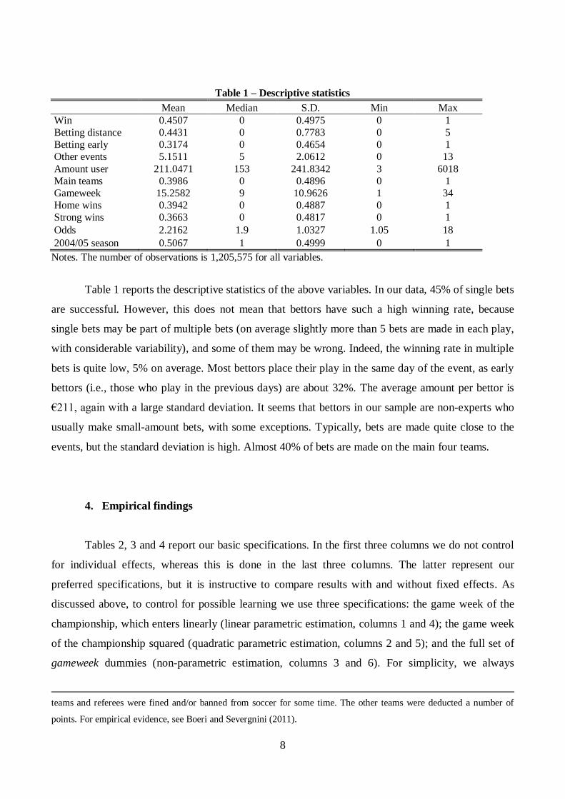
Table 1 – Descriptive statistics
Mean Median S.D. Min Max
Win 0.4507 0 0.4975 0 1
Betting distance 0.4431 0 0.7783 0 5
Betting early 0.3174 0 0.4654 0 1
Other events 5.1511 5 2.0612 0 13
Amount user 211.0471 153 241.8342 3 6018
Main teams 0.3986 0 0.4896 0 1
Gameweek 15.2582 9 10.9626 1 34
Home wins 0.3942 0 0.4887 0 1
Strong wins 0.3663 0 0.4817 0 1
Odds 2.2162 1.9 1.0327 1.05 18
2004/05 season 0.5067 1 0.4999 0 1
Notes. The number of observations is 1,205,575 for all variables.
Table 1 reports the descriptive statistics of the above variables. In our data, 45% of single bets
are successful. However, this does not mean that bettors have such a high winning rate, because
single bets may be part of multiple bets (on average slightly more than 5 bets are made in each play,
with considerable variability), and some of them may be wrong. Indeed, the winning rate in multiple
bets is quite low, 5% on average. Most bettors place their play in the same day of the event, as early
bettors (i.e., those who play in the previous days) are about 32%. The average amount per bettor is
€211, again with a large standard deviation. It seems that bettors in our sample are non-experts who
usually make small-amount bets, with some exceptions. Typically, bets are made quite close to the
events, but the standard deviation is high. Almost 40% of bets are made on the main four teams.
4. Empirical findings
Tables 2, 3 and 4 report our basic specifications. In the first three columns we do not control
for individual effects, whereas this is done in the last three columns. The latter represent our
preferred specifications, but it is instructive to compare results with and without fixed effects. As
discussed above, to control for possible learning we use three specifications: the game week of the
championship, which enters linearly (linear parametric estimation, columns 1 and 4); the game week
of the championship squared (quadratic parametric estimation, columns 2 and 5); and the full set of
gameweek dummies (non-parametric estimation, columns 3 and 6). For simplicity, we always
teams and referees were fined and/or banned from soccer for some time. The other teams were deducted a number of
points. For empirical evidence, see Boeri and Severgnini (2011).
9
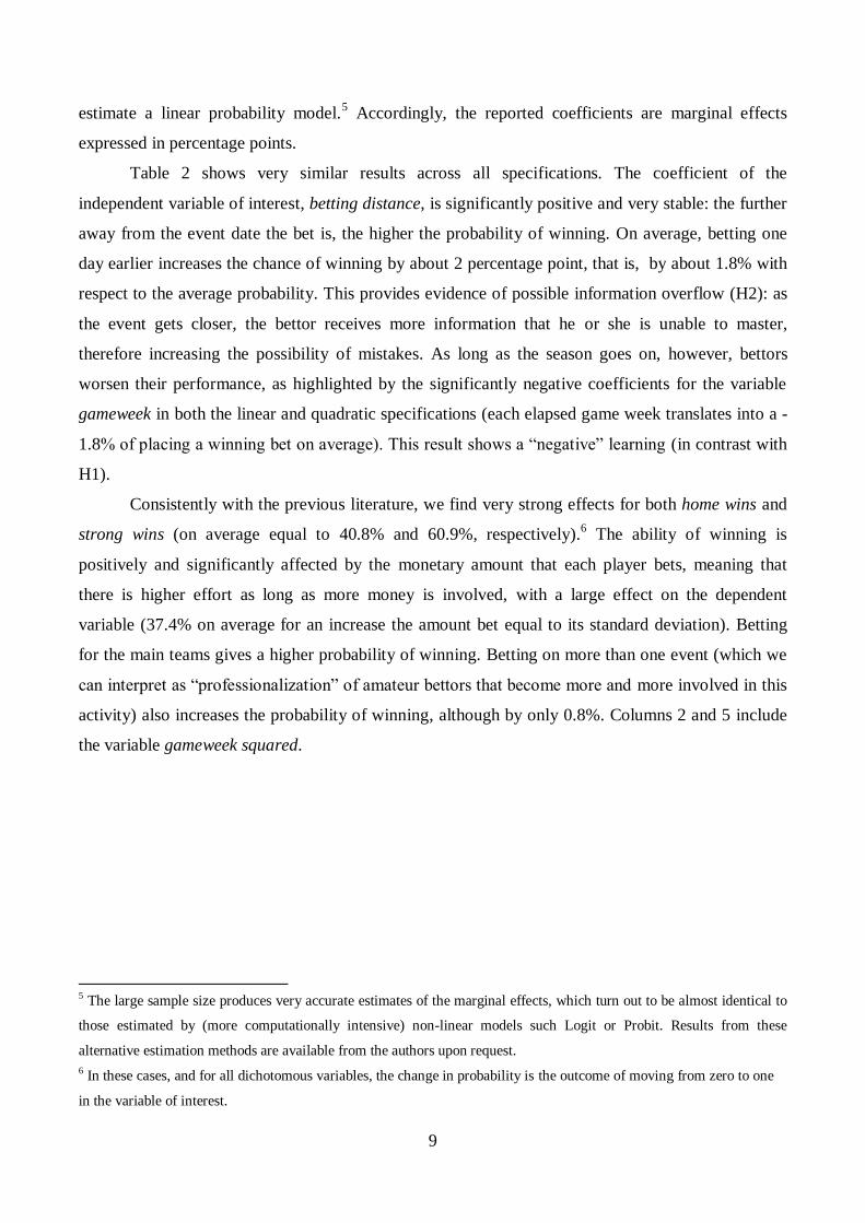
estimate a linear probability model.5 Accordingly, the reported coefficients are marginal effects
expressed in percentage points.
Table 2 shows very similar results across all specifications. The coefficient of the
independent variable of interest, betting distance, is significantly positive and very stable: the further
away from the event date the bet is, the higher the probability of winning. On average, betting one
day earlier increases the chance of winning by about 2 percentage point, that is, by about 1.8% with
respect to the average probability. This provides evidence of possible information overflow (H2): as
the event gets closer, the bettor receives more information that he or she is unable to master,
therefore increasing the possibility of mistakes. As long as the season goes on, however, bettors
worsen their performance, as highlighted by the significantly negative coefficients for the variable
gameweek in both the linear and quadratic specifications (each elapsed game week translates into a -
1.8% of placing a winning bet on average). This result shows a “negative” learning (in contrast with
H1).
Consistently with the previous literature, we find very strong effects for both home wins and
strong wins (on average equal to 40.8% and 60.9%, respectively).6 The ability of winning is
positively and significantly affected by the monetary amount that each player bets, meaning that
there is higher effort as long as more money is involved, with a large effect on the dependent
variable (37.4% on average for an increase the amount bet equal to its standard deviation). Betting
for the main teams gives a higher probability of winning. Betting on more than one event (which we
can interpret as “professionalization” of amateur bettors that become more and more involved in this
activity) also increases the probability of winning, although by only 0.8%. Columns 2 and 5 include
the variable gameweek squared.
5 The large sample size produces very accurate estimates of the marginal effects, which turn out to be almost identical to
those estimated by (more computationally intensive) non-linear models such Logit or Probit. Results from these
alternative estimation methods are available from the authors upon request.
6 In these cases, and for all dichotomous variables, the change in probability is the outcome of moving from zero to one
in the variable of interest.
10
Table 2 - Baseline specifications: distance from the event date (betting distance)
(1) (2) (3) (4) (5) (6)
Betting distance 0.008*** 0.008*** 0.007*** 0.008*** 0.008*** 0.008***
[0.001] [0.001] [0.001] [0.001] [0.001] [0.001]
Home wins 0.184*** 0.184*** 0.182*** 0.184*** 0.184*** 0.182***
[0.002] [0.002] [0.002] [0.001] [0.001] [0.001]
Strong wins 0.283*** 0.283*** 0.298*** 0.284*** 0.284*** 0.297***
[0.002] [0.002] [0.002] [0.001] [0.001] [0.001]
Gameweek -0.004*** -0.007***
-0.004*** -0.007***
[0.000] [0.000]
[0.000] [0.000]
Gameweek squared
0.000***
0.000***
[0.000]
[0.000]
Other events 0.007*** 0.008*** 0.007*** 0.007*** 0.007*** 0.007***
[0.000] [0.000] [0.000] [0.000] [0.000] [0.000]
Amount user 0.008 0.010* 0.006 0.008*** 0.010*** 0.006**
[0.005] [0.005] [0.003] [0.002] [0.002] [0.002]
Main teams 0.049*** 0.048*** 0.047*** 0.049*** 0.048*** 0.047***
[0.002] [0.002] [0.002] [0.001] [0.001] [0.001]
Odds -0.096*** -0.096*** -0.095*** -0.096*** -0.096*** -0.095***
[0.001] [0.001] [0.001] [0.000] [0.000] [0.000]
2004/05 season -0.013*** -0.030***
-0.014*** -0.031***
[0.004] [0.005]
[0.003] [0.003]
Gameweek dummies NO NO YES NO NO YES
Individual fixed effects NO NO NO YES YES YES
No. observations 1,205,575 1,205,575 1,205,575 1,205,575 1,205,575 1,205,575
No. individuals 7,093 7,093 7,093 7,093 7,093 7,093
Notes. Dependent variable: probability of correctly forecasting the single event (included in either a single or multiple
bet). Estimation method: linear probability model as in equation (1). P-values in brackets. Significance at the 5% level is
represented by ** and at the 1% level by ***.
We do not report its value since it is extremely small (in the order of four decimals); therefore
the linear specification is fairly good. The same applies to the following tables, when this variable is
included. As we would also expect, higher odds are related with a lower probability of winning (on
average by -46.0% for an increase of odds equal to its standard deviation).
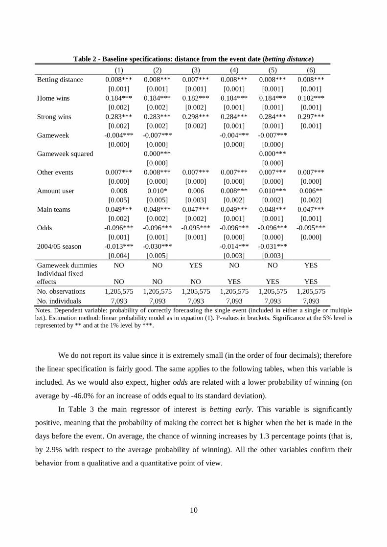
In Table 3 the main regressor of interest is betting early. This variable is significantly
positive, meaning that the probability of making the correct bet is higher when the bet is made in the
days before the event. On average, the chance of winning increases by 1.3 percentage points (that is,
by 2.9% with respect to the average probability of winning). All the other variables confirm their
behavior from a qualitative and a quantitative point of view.
11
Table 3 – Baseline specifications: betting before the event date (betting early)
(1) (2) (3) (4) (5) (6)
Betting early 0.013*** 0.013*** 0.011*** 0.013*** 0.013*** 0.011***
[0.001] [0.001] [0.001] [0.001] [0.001] [0.001]
Home wins 0.184*** 0.184*** 0.182*** 0.184*** 0.184*** 0.182***
[0.002] [0.002] [0.002] [0.001] [0.001] [0.001]
Strong wins 0.283*** 0.283*** 0.298*** 0.284*** 0.284*** 0.297***
[0.002] [0.002] [0.002] [0.001] [0.001] [0.001]
Gameweek -0.004*** -0.007***
-0.004*** -0.007***
[0.000] [0.000]
[0.000] [0.000]
Gameweek squared
0.000***
0.000***
[0.000]
[0.000]
Other events 0.008*** 0.008*** 0.007*** 0.007*** 0.008*** 0.007***
[0.000] [0.000] [0.000] [0.000] [0.000] [0.000]
Amount user 0.008 0.010* 0.006* 0.008*** 0.010*** 0.006**
[0.005] [0.005] [0.003] [0.002] [0.002] [0.002]
Main teams 0.048*** 0.048*** 0.047*** 0.049*** 0.048*** 0.047***
[0.002] [0.002] [0.002] [0.001] [0.001] [0.001]
Odds -0.096*** -0.096*** -0.095*** -0.096*** -0.096*** -0.095***
[0.001] [0.001] [0.001] [0.000] [0.000] [0.000]
2004/05 season -0.013*** -0.030***
-0.014*** -0.031***
[0.004] [0.005]
[0.003] [0.003]
Gameweek dummies NO NO YES NO NO YES
Individual fixed
effects NO NO NO YES YES YES
No. of observations 1,205,575 1,205,575 1,205,575 1,205,575 1,205,575 1,205,575
No. of individuals 7,093 7,093 7,093 7,093 7,093 7,093
Notes. Dependent variable: probability of correctly forecasting the single event (included in either a single or multiple
bet). Estimation method: linear probability model as in equation (1). P-values in brackets. Significance at the 5% level is represented by ** and at the 1% level by ***.
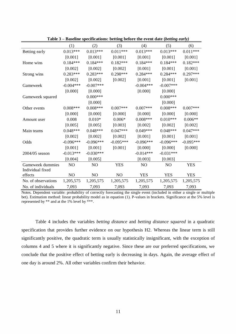
Table 4 includes the variables betting distance and betting distance squared in a quadratic
specification that provides further evidence on our hypothesis H2. Whereas the linear term is still
significantly positive, the quadratic term is usually statistically insignificant, with the exception of
columns 4 and 5 where it is significantly negative. Since these are our preferred specifications, we
conclude that the positive effect of betting early is decreasing in days. Again, the average effect of
one day is around 2%. All other variables confirm their behavior.
12
Table 4 – Alternative specifications: quadratic distance from the event date
(1) (2) (3) (4) (5) (6)
Betting distance 0.010*** 0.009*** 0.007*** 0.010*** 0.010*** 0.007***
[0.002] [0.002] [0.001] [0.001] [0.001] [0.001]
Betting distance squared -0.001 -0.001 0.000 -0.001** -0.001* 0.000
[0.001] [0.001] [0.001] [0.000] [0.000] [0.000]
Home wins 0.184*** 0.184*** 0.182*** 0.184*** 0.184*** 0.182***
[0.002] [0.002] [0.002] [0.001] [0.001] [0.001]
Strong wins 0.283*** 0.283*** 0.298*** 0.284*** 0.284*** 0.297***
[0.002] [0.002] [0.002] [0.001] [0.001] [0.001]
Gameweek -0.004*** -0.007***
-0.004*** -0.007***
[0.000] [0.000]
[0.000] [0.000]
Gameweek squared
0.000***
0.000***
[0.000]
[0.000]
Other events 0.007*** 0.008*** 0.007*** 0.007*** 0.007*** 0.007***
[0.000] [0.000] [0.000] [0.000] [0.000] [0.000]
Amount user 0.008 0.010* 0.006 0.008*** 0.010*** 0.006**
[0.005] [0.005] [0.003] [0.002] [0.002] [0.002]
Main teams 0.048*** 0.048*** 0.047*** 0.049*** 0.048*** 0.047***
[0.002] [0.002] [0.002] [0.001] [0.001] [0.001]
Odds -0.096*** -0.096*** -0.095*** -0.096*** -0.096*** -0.095***
[0.001] [0.001] [0.001] [0.000] [0.000] [0.000]
2004/05 season -0.013*** -0.030***
-0.014*** -0.031***
[0.004] [0.005]
[0.003] [0.003]
Gameweek dummies NO NO YES NO NO YES
Individual fixed effects NO NO NO YES YES YES
No. of observations 1,205,575 1,205,575 1,205,575 1,205,575 1,205,575 1,205,575
No. of individuals 7,093 7,093 7,093 7,093 7,093 7,093
Notes. Dependent variable: probability of correctly forecasting the single event (included in either a single or multiple bet).
Estimation method: linear probability model as in equation (1), with the addition of the regressor betting distance squared. P-
values in brackets. Significance at the 5% level is represented by ** and at the 1% level by ***.
The last three tables address some heterogeneity issues, that is, they assess whether the timing
effect is stronger in some specific subsamples. This is meant to further evaluate our information-
overflow interpretation of the “betting early” effect we identify in our data.
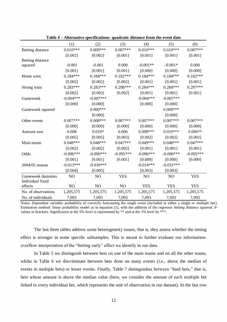
In Table 5 we distinguish between bets on one of the main teams and on all the other teams,
whilst in Table 6 we discriminate between bets done on many events (i.e., above the median of
events in multiple bets) or lesser events. Finally, Table 7 distinguishes between “hard bets,” that is,
bets whose amount is above the median value (here, we consider the amount of each multiple bet
linked to every individual bet, which represents the unit of observation in our dataset). In the last row
13
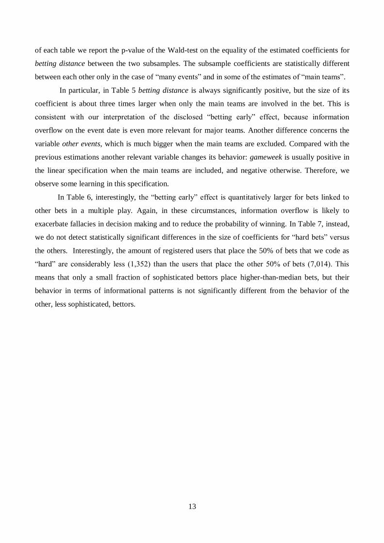
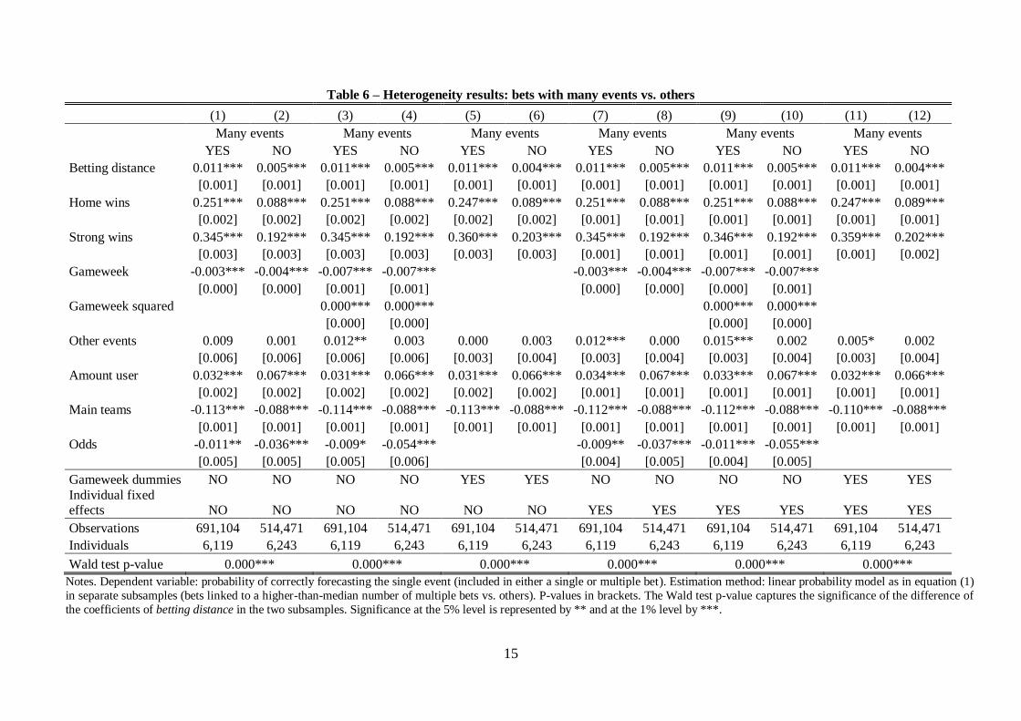
of each table we report the p-value of the Wald-test on the equality of the estimated coefficients for
betting distance between the two subsamples. The subsample coefficients are statistically different
between each other only in the case of “many events” and in some of the estimates of “main teams”.
In particular, in Table 5 betting distance is always significantly positive, but the size of its
coefficient is about three times larger when only the main teams are involved in the bet. This is
consistent with our interpretation of the disclosed “betting early” effect, because information
overflow on the event date is even more relevant for major teams. Another difference concerns the
variable other events, which is much bigger when the main teams are excluded. Compared with the
previous estimations another relevant variable changes its behavior: gameweek is usually positive in
the linear specification when the main teams are included, and negative otherwise. Therefore, we
observe some learning in this specification.
In Table 6, interestingly, the “betting early” effect is quantitatively larger for bets linked to
other bets in a multiple play. Again, in these circumstances, information overflow is likely to
exacerbate fallacies in decision making and to reduce the probability of winning. In Table 7, instead,
we do not detect statistically significant differences in the size of coefficients for “hard bets” versus
the others. Interestingly, the amount of registered users that place the 50% of bets that we code as
“hard” are considerably less (1,352) than the users that place the other 50% of bets (7,014). This
means that only a small fraction of sophisticated bettors place higher-than-median bets, but their
behavior in terms of informational patterns is not significantly different from the behavior of the
other, less sophisticated, bettors.
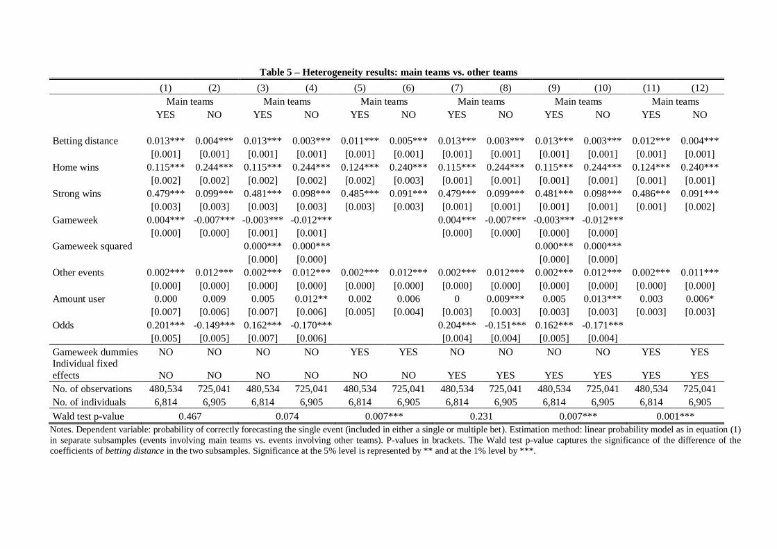
Table 5 – Heterogeneity results: main teams vs. other teams
(1) (2) (3) (4) (5) (6) (7) (8) (9) (10) (11) (12)
Main teams Main teams Main teams Main teams Main teams Main teams
YES NO YES NO YES NO YES NO YES NO YES NO
Betting distance 0.013*** 0.004*** 0.013*** 0.003*** 0.011*** 0.005*** 0.013*** 0.003*** 0.013*** 0.003*** 0.012*** 0.004***
[0.001] [0.001] [0.001] [0.001] [0.001] [0.001] [0.001] [0.001] [0.001] [0.001] [0.001] [0.001]
Home wins 0.115*** 0.244*** 0.115*** 0.244*** 0.124*** 0.240*** 0.115*** 0.244*** 0.115*** 0.244*** 0.124*** 0.240***
[0.002] [0.002] [0.002] [0.002] [0.002] [0.003] [0.001] [0.001] [0.001] [0.001] [0.001] [0.001]
Strong wins 0.479*** 0.099*** 0.481*** 0.098*** 0.485*** 0.091*** 0.479*** 0.099*** 0.481*** 0.098*** 0.486*** 0.091***
[0.003] [0.003] [0.003] [0.003] [0.003] [0.003] [0.001] [0.001] [0.001] [0.001] [0.001] [0.002]
Gameweek 0.004*** -0.007*** -0.003*** -0.012***
0.004*** -0.007*** -0.003*** -0.012***
[0.000] [0.000] [0.001] [0.001]
[0.000] [0.000] [0.000] [0.000]
Gameweek squared
0.000*** 0.000***
0.000*** 0.000***
[0.000] [0.000]
[0.000] [0.000]
Other events 0.002*** 0.012*** 0.002*** 0.012*** 0.002*** 0.012*** 0.002*** 0.012*** 0.002*** 0.012*** 0.002*** 0.011***
[0.000] [0.000] [0.000] [0.000] [0.000] [0.000] [0.000] [0.000] [0.000] [0.000] [0.000] [0.000]
Amount user 0.000 0.009 0.005 0.012** 0.002 0.006 0 0.009*** 0.005 0.013*** 0.003 0.006*
[0.007] [0.006] [0.007] [0.006] [0.005] [0.004] [0.003] [0.003] [0.003] [0.003] [0.003] [0.003]
Odds 0.201*** -0.149*** 0.162*** -0.170***
0.204*** -0.151*** 0.162*** -0.171***
[0.005] [0.005] [0.007] [0.006]
[0.004] [0.004] [0.005] [0.004]
Gameweek dummies NO NO NO NO YES YES NO NO NO NO YES YES Individual fixed
effects NO NO NO NO NO NO YES YES YES YES YES YES
No. of observations 480,534 725,041 480,534 725,041 480,534 725,041 480,534 725,041 480,534 725,041 480,534 725,041
No. of individuals 6,814 6,905 6,814 6,905 6,814 6,905 6,814 6,905 6,814 6,905 6,814 6,905
Wald test p-value 0.467 0.074 0.007*** 0.231 0.007*** 0.001***
Notes. Dependent variable: probability of correctly forecasting the single event (included in either a single or multiple bet). Estimation method: linear probability model as in equation (1)
in separate subsamples (events involving main teams vs. events involving other teams). P-values in brackets. The Wald test p-value captures the significance of the difference of the
coefficients of betting distance in the two subsamples. Significance at the 5% level is represented by ** and at the 1% level by ***.
15
Table 6 – Heterogeneity results: bets with many events vs. others
(1) (2) (3) (4) (5) (6) (7) (8) (9) (10) (11) (12)
Many events Many events Many events Many events Many events Many events
YES NO YES NO YES NO YES NO YES NO YES NO
Betting distance 0.011*** 0.005*** 0.011*** 0.005*** 0.011*** 0.004*** 0.011*** 0.005*** 0.011*** 0.005*** 0.011*** 0.004***
[0.001] [0.001] [0.001] [0.001] [0.001] [0.001] [0.001] [0.001] [0.001] [0.001] [0.001] [0.001]
Home wins 0.251*** 0.088*** 0.251*** 0.088*** 0.247*** 0.089*** 0.251*** 0.088*** 0.251*** 0.088*** 0.247*** 0.089***
[0.002] [0.002] [0.002] [0.002] [0.002] [0.002] [0.001] [0.001] [0.001] [0.001] [0.001] [0.001]
Strong wins 0.345*** 0.192*** 0.345*** 0.192*** 0.360*** 0.203*** 0.345*** 0.192*** 0.346*** 0.192*** 0.359*** 0.202***
[0.003] [0.003] [0.003] [0.003] [0.003] [0.003] [0.001] [0.001] [0.001] [0.001] [0.001] [0.002]
Gameweek -0.003*** -0.004*** -0.007*** -0.007***
-0.003*** -0.004*** -0.007*** -0.007***
[0.000] [0.000] [0.001] [0.001]
[0.000] [0.000] [0.000] [0.001]
Gameweek squared
0.000*** 0.000***
0.000*** 0.000***
[0.000] [0.000]
[0.000] [0.000]
Other events 0.009 0.001 0.012** 0.003 0.000 0.003 0.012*** 0.000 0.015*** 0.002 0.005* 0.002
[0.006] [0.006] [0.006] [0.006] [0.003] [0.004] [0.003] [0.004] [0.003] [0.004] [0.003] [0.004]
Amount user 0.032*** 0.067*** 0.031*** 0.066*** 0.031*** 0.066*** 0.034*** 0.067*** 0.033*** 0.067*** 0.032*** 0.066***
[0.002] [0.002] [0.002] [0.002] [0.002] [0.002] [0.001] [0.001] [0.001] [0.001] [0.001] [0.001]
Main teams -0.113*** -0.088*** -0.114*** -0.088*** -0.113*** -0.088*** -0.112*** -0.088*** -0.112*** -0.088*** -0.110*** -0.088***
[0.001] [0.001] [0.001] [0.001] [0.001] [0.001] [0.001] [0.001] [0.001] [0.001] [0.001] [0.001]
Odds -0.011** -0.036*** -0.009* -0.054***
-0.009** -0.037*** -0.011*** -0.055***
[0.005] [0.005] [0.005] [0.006]
[0.004] [0.005] [0.004] [0.005]
Gameweek dummies NO NO NO NO YES YES NO NO NO NO YES YES
Individual fixed effects NO NO NO NO NO NO YES YES YES YES YES YES
Observations 691,104 514,471 691,104 514,471 691,104 514,471 691,104 514,471 691,104 514,471 691,104 514,471
Individuals 6,119 6,243 6,119 6,243 6,119 6,243 6,119 6,243 6,119 6,243 6,119 6,243
Wald test p-value 0.000*** 0.000*** 0.000*** 0.000*** 0.000*** 0.000***
Notes. Dependent variable: probability of correctly forecasting the single event (included in either a single or multiple bet). Estimation method: linear probability model as in equation (1)
in separate subsamples (bets linked to a higher-than-median number of multiple bets vs. others). P-values in brackets. The Wald test p-value captures the significance of the difference of
the coefficients of betting distance in the two subsamples. Significance at the 5% level is represented by ** and at the 1% level by ***.
16
Table 7 – Heterogeneity results: bets involving larger-than-median amounts vs. others
(1) (2) (3) (4) (5) (6) (7) (8) (9) (10) (11) (12)
Hard bets Hard bets Hard bets Hard bets Hard bets Hard bets
YES NO YES NO YES NO YES NO YES NO YES NO
Betting distance 0.008*** 0.008*** 0.008*** 0.008*** 0.007*** 0.008*** 0.008*** 0.008*** 0.008*** 0.008*** 0.007*** 0.009***
[0.001] [0.001] [0.001] [0.001] [0.001] [0.001] [0.001] [0.001] [0.001] [0.001] [0.001] [0.001]
Home wins 0.184*** 0.184*** 0.184*** 0.184*** 0.182*** 0.182*** 0.184*** 0.184*** 0.184*** 0.184*** 0.182*** 0.183***
[0.003] [0.002] [0.003] [0.002] [0.003] [0.002] [0.001] [0.001] [0.001] [0.001] [0.001] [0.001]
Strong wins 0.295*** 0.274*** 0.295*** 0.274*** 0.311*** 0.284*** 0.295*** 0.274*** 0.295*** 0.274*** 0.311*** 0.284***
[0.004] [0.003] [0.004] [0.003] [0.004] [0.003] [0.001] [0.001] [0.001] [0.001] [0.001] [0.001]
Gameweek -0.003*** -0.004*** -0.008*** -0.007***
-0.003*** -0.005*** -0.008*** -0.007***
[0.000] [0.000] [0.001] [0.001]
[0.000] [0.000] [0.000] [0.000]
Gameweek squared
0.000*** 0.000***
0.000*** 0.000***
[0.000] [0.000]
[0.000] [0.000]
Other events 0.007*** 0.008*** 0.007*** 0.008*** 0.007*** 0.008*** 0.006*** 0.008*** 0.007*** 0.008*** 0.007*** 0.008***
[0.000] [0.000] [0.000] [0.000] [0.000] [0.000] [0.000] [0.000] [0.000] [0.000] [0.000] [0.000]
Amount user 0.043*** 0.054*** 0.042*** 0.053*** 0.041*** 0.053*** 0.043*** 0.055*** 0.042*** 0.054*** 0.041*** 0.053***
[0.003] [0.002] [0.003] [0.002] [0.003] [0.002] [0.001] [0.001] [0.001] [0.001] [0.001] [0.001]
Main teams -0.094*** -0.097*** -0.094*** -0.097*** -0.094*** -0.097*** -0.094*** -0.097*** -0.094*** -0.097*** -0.094*** -0.096***
[0.001] [0.001] [0.001] [0.001] [0.001] [0.001] [0.001] [0.001] [0.001] [0.001] [0.001] [0.001]
Odds 0.008 -0.032*** -0.018** -0.045***
0.007* -0.039*** -0.020*** -0.051***
[0.008] [0.005] [0.008] [0.006]
[0.004] [0.004] [0.005] [0.005]
Gameweek dummies NO NO NO NO YES YES NO NO NO NO YES YES
Individual fixed effects NO NO NO NO NO NO YES YES YES YES YES YES
No. of observations 596,037 609,538 596,037 609,538 596,037 609,538 596,037 609,538 596,037 609,538 596,037 609,538
No. of individuals 1,352 7,014 1,352 7,014 1,352 7,014 1,352 7,014 1,352 7,014 1,352 7,014
Wald test p-value 0.936 0.991 0.366 0.464 0.405 0.679
Notes. Dependent variable: probability of correctly forecasting the single event (included in either a single or multiple bet). Estimation method: linear probability model as in equation
(1) in separate subsamples (bets involving a higher-than-median amount of the multiple bet vs. others). P-values in brackets. The Wald test p-value captures the significance of the
difference of the coefficients of betting distance in the two subsamples. Significance at the 5% level is represented by ** and at the 1% level by ***.
5. Conclusion
We have analyzed more than 1,250,000 bets on Italian soccer matches to test if bettors
improve their winning percentage with respect to the timing of each bet. We do not find evidence of
improvement in bettors' performance attributable to learning. Even more, their performance gets
worse as the season moves forward. More interestingly, we find that betting timing matters. We
obtain a small but statistically significant difference in the winning probability of early bettors versus
late bettors. The poorer forecasting performance of later bettors is attributed to an inefficient
processing of information, also consistent with the heterogeneity results that we are able to disclose
thanks to the richness of the data.
The late bettors' decision process is affected by various cues that, unknown to the earlier
bettors, have scarce relevance for predicting the outcomes. The excess of noisy information
(especially harsh if the same individual decides to bet on the main teams or on multiple events)
reduces the possibility of using very simple prediction methods, such as team rankings or home team
winning. Moreover, the use of these criteria and cues greatly improves the possibility of placing a
winning bet. Our findings support the hypothesis that forecasting activity is negatively affected when
the number of cues is too large in comparison with information processing capacity, and provide an
explanation to the fact that in betting simple prediction rules usually perform better than models
based on extensive knowledge.
References
Anderson, P., Edman, J., and Ekman, M. (2005). Predicting the World Cup 2002 in soccer:
Performance and confidence of experts and non-experts. International Journal of
Forecasting, 21, 565–576.
Asch, P., Malkiel B. G., and Quandt, R. E. (1984). Market efficiency in racetrack betting. The
Journal of Business, 57, 165–175.
Barber, B. M., and Odean, T. (2002). Online investors: Do the slow die first?. The Review of
Financial Studies, 15, 455-487.
Benartzi, S., and Thaler, R. (2001). Naive diversification strategies in retirement saving plans.
American Economic Review, 91, 79–98.
Bettman, J. R., Johnson, E. J., Luce, M. F., and Payne, J. W. (1993). Correlation, conflict, and
choice. Journal of Experimental Psychology: Learning, Memory, and Cognition, 19, 931-
951.
Bichler, U. W., and Butler, M. (2007). Information economics. London: Routledge.
Boeri, T., and Severgnini, B. (2011), Match rigging and the career concerns of referees. Labour, 18,
349–359.
18
Boulier, B. L., and Stekler, H. O. (1999). Are sports seedings good predictors? An evaluation.
International Journal of Forecasting, 15, 83–91.
Boulier, B. L., and Stekler, H. O. (2003). Predicting the outcomes of National Footbal League
games. International Journal of Forecasting, 19, 257–270.
Camerer, C. F., and Johnson, E. J. (1991). The process–performance paradox in expert judgment:
How can experts know so much and predict so badly? In K. A. Ericsson, & J. Smith (Eds.),
Toward a general theory of expertise: Prospects and limits. New York: Cambridge Press,
195–217.
Crafts, N. F. R. (1985). Some evidence of insider knowledge in horse race betting in Britain.
Economica, 52, 295–304
Crawford, V. P., and Sobel, J. (1982). Strategic information transmission. Econometrica, 50, 1431–
1451.
Davis, F. D., Lohse, G. L., and Kottemann, J. E. (1994). Harmful effects of seemingly helpful
information on forecasts of stock earnings. Journal of Economic Psychology, 15, 253–267.
Dieckmann, A. and Rieskamp, J. (2007). The influence of information redundancy on probabilistic
inferences. Memory & Cognition, 35, 1801–1813.
Einhorn, H. J., and Hogarth, R. M. (1975). Unit weighting schemes for decision making.
Organizational Behavior and Human Performance, 13, 171–192.
Figlewski, S. (1979). Subjective information and market efficiency in a betting market. Journal of
Political Economy, 87, 75–88.
Forrest, D., and Simmons, R. (2000). Forecasting sport: the behaviour and performance of football
tipsters. International Journal of Forecasting, 16, 317–331.
Gigerenzer, G., and Todd, P. M., and the ABC Research Group (1999). Simple heuristics that make
us smart. New York: Oxford University Press.
Glickman, M. E., and Stern, H. S. (1998). A state-space model for emphasis on forecast evaluations.
national football league scores. Journal of the American Statistical Association, 93, 25–35.
Goldstein, D. G. and Gigerenzer, G. (2009). Fast and frugal forecasting. International Journal of
Forecasting, 25, 760-772.
Hausch, D. B., Ziemba, W. T., and Rubinstein, M. (1981). Efficiency of the market for racetrack
betting. Management Science, 27, 1435–1452.
Johnson, J. G., and Raab, M. (2003). Take the first: Option-generation and resulting choices.
Organizational Behavior and Human Decision Processes, 91, 215–229.
Kahneman, D., and Tversky, A. (1973). On the psychology of prediction. Psychological Review, 80,
237–251.
Klein, G., Wolf, S., Militello, L., and Zsambok, C. (1995). Characteristics of skilled option
generation in chess. Organizational Behavior and Human Decision Processes, 62, 63–69.
Martignon, L., and Hoffrage, U. (2002). Fast, frugal, and fit: Simple heuristics for paired
comparison. Theory and Decision, 52, 29–71.
Newell, B. R., and Shanks, D. R. (2004). On the role of recognition in decision making. Journal of
Experimental Psychology. Learning, Memory, and Cognition, 30, 923–935.
Oskamp, S. (1965). Overconfidence in case-study judgments. The Journal of Consulting Psychology,
2, 261–265.
Pope, P. F., & Peel, D. A. (1989). Information, prices and efficiency in a fixed-odds betting market.
Economica 56, 323–341.
Preston, M. G. and Baratta, P. (1948). An experimental study of the auction value of an uncertain
outcome. American Journal of Psychology, 61, 183–93.
Rieskamp, J., and Otto, P. E. (2006). SSL: A theory of how people learn to select strategies. Journal
of Experimental Psychology: General, 135, 207–236.
Sauer, R. D. 1998. The economics of wagering markets. Journal of Economic Literature, 36, 2021–
2064.

19
Snyder, W. W. (1978) Testing the efficient markets model, The Journal of Finance, 33, 1109-1118.
Thaler, R., and Ziemba, W. (1988). Parimutuel betting markets: Racetracks and lotteries. Journal of
Economic Perspectives, 2, 161–174.
Williams, L. V. (1999), Information efficiency in betting markets. A Survey, Bulletin of Economic
Research 51, 307-337.
Yaari, M. E. (1965). Convexity in the theory of choice under risk. Quarterly Journal of Economics,
79, 278–90.
LabSi Working Papers
ISSN 1825-8131 (online version) 1825-8123 (print version)
Issue Author Title
n. 1/2005 Roberto Galbiati Pietro Vertova
Law and Behaviours in Social Dilemmas: Testing the Effect of Obligations on Cooperation (April 2005)
n. 2/2005
Marco Casari Luigi Luini
Group Cooperation Under Alternative Peer Punish-ment Technologies: An Experiment (June 2005)
n. 3/2005 Carlo Altavilla Luigi Luini Patrizia Sbriglia
Social Learning in Market Games (June 2005)
n. 4/2005 Roberto Ricciuti Bringing Macroeconomics into the Lab (December 2005)
n. 5/2006 Alessandro Innocenti Maria Grazia Pazienza
Altruism and Gender in the Trust Game (February 2006)
n. 6/2006 Brice Corgnet Angela Sutan Arvind Ashta
The power of words in financial markets:soft ver-sus hard communication, a strategy method experi-ment (April 2006)
n. 7/2006 Brian Kluger Daniel Friedman
Financial Engineering and Rationality: Experimental Evidence Based on the Monty Hall Problem (April 2006)
n. 8/2006 Gunduz Caginalp Vladimira Ilieva
The dynamics of trader motivations in asset bub-bles (April 2006)
n. 9/2006 Gerlinde Fellner Erik Theissen
Short Sale Constraints, Divergence of Opinion and Asset Values: Evidence from the Laboratory (April 2006)
n. 10/2006
Robin Pope Reinhard Selten Sebastian Kube Jürgen von Hagen
Experimental Evidence on the Benefits of Eliminat-ing Exchange Rate Uncertainties and Why Expected Utility Theory causes Economists to Miss Them (May 2006)
n. 11/2006 Niall O'Higgins Patrizia Sbriglia
Are Imitative Strategies Game Specific? Experimen-tal Evidence from Market Games (October 2006)
n. 12/2007 Mauro Caminati Alessandro Innocenti Roberto Ricciuti
Drift and Equilibrium Selection with Human and Virtual Players (April 2007)
n. 13/2007 Klaus Abbink Jordi Brandts
Political Autonomy and Independence: Theory and Experimental Evidence (September 2007)
n. 14/2007 Jens Großer Arthur Schram
Public Opinion Polls, Voter Turnout, and Welfare: An Experimental Study (September 2007)
n. 15/2007 Nicolao Bonini Ilana Ritov Michele Graffeo
When does a referent problem affect willingness to pay for a public good? (September 2007)
n. 16/2007 Jaromir Kovarik Belief Formation and Evolution in Public Good Games (September 2007)
n. 17/2007 Vivian Lei Steven Tucker Filip Vesely
Forgive or Buy Back: An Experimental Study of Debt Relief (September 2007)
n. 18/2007 Joana Pais Ágnes Pintér
School Choice and Information. An Experimental Study on Matching Mechanisms (September 2007)
n. 19/2007
Antonio Cabrales Rosemarie Nagel José V. Rodrìguez Mora
It is Hobbes not Rousseau: An Experiment on Social Insurance (September 2007)
n. 20/2008 Carla Marchese Marcello Montefiori
Voting the public expenditure: an experiment (May 2008)
n. 21/2008 Francesco Farina Niall O’Higgins Patrizia Sbriglia
Eliciting motives for trust and reciprocity by attitudi-nal and behavioural measures (June 2008)
n. 22/2008 Alessandro Innocenti Alessandra Rufa Jacopo Semmoloni
Cognitive Biases and Gaze Direction: An Experimen-tal Study (June 2008)
n. 23/2008 Astri Hole Drange How do economists differ from others in distributive situations? (September 2008)
n. 24/2009 Roberto Galbiati Karl Schlag Joël van der Weele
Can Sanctions Induce Pessimism? An Experiment (January 2009)
n. 25/2009 Annamaria Nese Patrizia Sbriglia
Individuals’ Voting Choice and Cooperation in Re-peated Social Dilemma Games (February 2009)
n. 26/2009 Alessandro Innocenti Antonio Nicita
Virtual vs. Standard Strike: An Experiment (June 2009)
n. 27/2009
Alessandro Innocenti Patrizia Lattarulo Maria Grazia Pazien-za
Heuristics and Biases in Travel Mode Choice (December 2009)
n. 28/2010 S.N. O’Higgins Arturo Palomba Patrizia Sbriglia
Second Mover Advantage and Bertrand Dynamic Competition: An Experiment (May 2010)
n. 29/2010
Valeria Faralla Francesca Benuzzi Paolo Nichelli Nicola Dimitri
Gains and Losses in Intertemporal Preferences: A Behavioural Study (June 2010)
n. 30/2010
Angela Dalton Alan Brothers Stephen Walsh Paul Whitney
Expert Elicitation Method Selection Process and Method Comparison (September 2010)
n. 31/2010 Giuseppe Attanasi Aldo Montesano
The Price for Information about Probabilities and its Relation with Capacities (September 2010)
n. 32/2010 Georgios Halkias Flora Kokkinaki
Attention, Memory, and Evaluation of Schema Incon-gruent Brand Messages: An Empirical Study (September 2010)
n. 33/2010
Valeria Faralla Francesca Benuzzi Fausta Lui Patrizia Baraldi Paolo Nichelli Nicola Dimitri
Gains and Losses: A Common Neural Network for Economic Behaviour (September 2010)
n. 34/2010 Jordi Brandts Orsola Garofalo
Gender Pairings and Accountability Effect (November 2010)
n. 35/2011 Ladislav Čaklović Conflict Resolution. Risk-As-Feelings Hypothesis.(January 2011)
n. 36/2011 Alessandro Innocenti Chiara Rapallini
Voting by Ballots and Feet in the Laboratory (January 2011)
n. 37/2011 Alessandro Innocenti Tommaso Nannicini Roberto Ricciutiì
The Importance of Betting Early (January 2012)

LABSI WORKING PAPERS
ISSN 1825-8131 (ONLINE VERSION) 1825-8123 (PRINT VERSION)
LABSI EXPERIMENTAL ECONOMICS LABORATORY UNIVERSITY OF SIENA
PIAZZA S. FRANCESCO, 7 53100 SIENA (ITALY)
http://www.labsi.org [email protected]