lag time in water quality response to best management ... time in water quality... · expectations...

85

Nonpoint source (NPS) watershed projects often fail to meet expectations for water quality improvement because of lag time, the time elapsed between adoption of management changes and the detection of measurable improvement in water quality in the target water body. Even when management changes are well-designed and fully implemented, water quality monitoring eff orts may not show defi nitive results if the monitoring period, program design, and sampling frequency are not suffi cient to address the lag between treatment and response. Th e main components of lag time include the time required for an installed practice to produce an eff ect, the time required for the eff ect to be delivered to the water resource, the time required for the water body to respond to the eff ect, and the eff ectiveness of the monitoring program to measure the response. Th e objectives of this review are to explore the characteristics of lag time components, to present examples of lag times reported from a variety of systems, and to recommend ways for managers to cope with the lag between treatment and response. Important processes infl uencing lag time include hydrology, vegetation growth, transport rate and path, hydraulic residence time, pollutant sorption properties, and ecosystem linkages. Th e magnitude of lag time is highly site and pollutant specifi c, but may range from months to years for relatively short-lived contaminants such as indicator bacteria, years to decades for excessive P levels in agricultural soils, and decades or more for sediment accumulated in river systems. Groundwater travel time is also an important contributor to lag time and may introduce a lag of decades between changes in agricultural practices and improvement in water quality. Approaches to deal with the inevitable lag between implementation of management practices and water quality response lie in appropriately characterizing the watershed, considering lag time in selection, siting, and monitoring of management measures, selection of appropriate indicators, and designing eff ective monitoring programs to detect water quality response.

Lag Time in Water Quality Response to Best Management Practices: A Review

Donald W. Meals,* and Steven A. Dressing Tetra Tech, Inc.

Thomas E. Davenport U.S. Environmental Protection Agency

Over the past four decades, most watershed NPS projects

have reported little or no improvement in water quality

even after extensive implementation of conservation measures or

best management practices (BMPs) in the watershed. Examples

include the Lower Kissimmee River Basin in Florida, the Conestoga

Headwaters in Pennsylvania, Oakwood Lakes-Poinsett in South

Dakota, and Vermont’s LaPlatte River Watershed and St. Albans

Bay Watershed (Gunsalus et al., 1992; Koerkle, 1992; Goodman et

al., 1992; Gale et al., 1993; Meals, 1993,1996; Jokela et al., 2004).

Numerous factors contribute to the failure of such projects to

achieve water quality objectives, including insuffi cient landowner

participation, uncooperative weather, improper selection of BMPs

or selection of BMPs for other than water quality purposes, mistakes

in understanding of pollution sources, poor experimental design,

and inadequate level or distribution of BMPs.

One important reason NPS watershed projects may fail to meet

expectations for water quality improvement is lag time. Lag time is

an inherent characteristic of the natural and altered systems under

study that may be generally defi ned as the amount of time between

an action and the response to that action. For this analysis, we defi ne

lag time as the time elapsed between installation or adoption of man-

agement measures at the level projected to reduce NPS pollution and

the fi rst measurable improvement in water quality in the target water

body. Installation refers to the completion of the construction phase

for structural practices. Adoption refers to the full use of an installed

physical practice or management practice such as nutrient manage-

ment. Even in cases where a program of management measures is

well designed and fully implemented, water quality monitoring ef-

forts—even those designed to be “long-term”—may not show defi ni-

tive results if the monitoring period and sampling frequency are not

suffi cient to address the lag between treatment and response.

Th e objectives of this review are to explore the important com-

ponents of lag time, to present examples of lag times reported

from a variety of geographic regions and water resource settings,

and to recommend ways for managers to cope with the lag be-

tween treatment and response in watershed projects.

Elements of Lag TimeProject management, system, and eff ects measurement com-

ponents can be important determinants of lag between treatment

Abbreviations: BMP, best management practice; NNPSMP, National Nonpoint Source

Monitoring Program; NPS, nonpoint source.

D.W. Meals, Tetra Tech, Inc., 84 Caroline St., Burlington, VT 05401. S.A. Dressing, Tetra

Tech, Inc., 1799 Rampart Dr., Alexandria, VA 22308. T.E. Davenport, U.S Environmental

Protection Agency, Region 5, 77 W. Jackson Blvd., Chicago, IL 60604.

Copyright © 2010 by the American Society of Agronomy, Crop Science

Society of America, and Soil Science Society of America. All rights

reserved. No part of this periodical may be reproduced or transmitted

in any form or by any means, electronic or mechanical, including pho-

tocopying, recording, or any information storage and retrieval system,

without permission in writing from the publisher.

Published in J. Environ. Qual. 39:85–96 (2010).

doi:10.2134/jeq2009.0108

Published online 13 Nov. 2009.

Received 20 Mar. 2009.

*Corresponding author ([email protected]).

© ASA, CSSA, SSSA

677 S. Segoe Rd., Madison, WI 53711 USA

REVIEWS AND ANALYSES

86 Journal of Environmental Quality • Volume 39 • January–February 2010

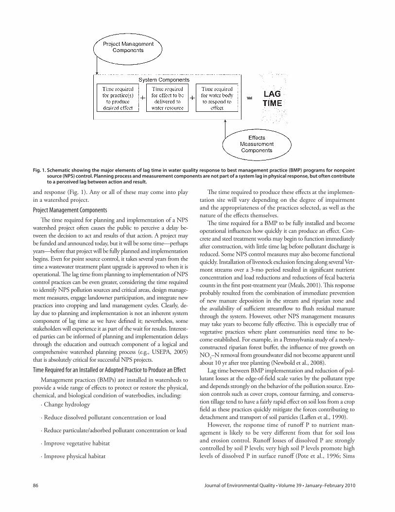
and response (Fig. 1). Any or all of these may come into play

in a watershed project.

Project Management Components

Th e time required for planning and implementation of a NPS

watershed project often causes the public to perceive a delay be-

tween the decision to act and results of that action. A project may

be funded and announced today, but it will be some time—perhaps

years—before that project will be fully planned and implementation

begins. Even for point source control, it takes several years from the

time a wastewater treatment plant upgrade is approved to when it is

operational. Th e lag time from planning to implementation of NPS

control practices can be even greater, considering the time required

to identify NPS pollution sources and critical areas, design manage-

ment measures, engage landowner participation, and integrate new

practices into cropping and land management cycles. Clearly, de-

lay due to planning and implementation is not an inherent system

component of lag time as we have defi ned it; nevertheless, some

stakeholders will experience it as part of the wait for results. Interest-

ed parties can be informed of planning and implementation delays

through the education and outreach component of a logical and

comprehensive watershed planning process (e.g., USEPA, 2005)

that is absolutely critical for successful NPS projects.

Time Required for an Installed or Adopted Practice to Produce an Eff ect

Management practices (BMPs) are installed in watersheds to

provide a wide range of eff ects to protect or restore the physical,

chemical, and biological condition of waterbodies, including:

· Change hydrology

· Reduce dissolved pollutant concentration or load

· Reduce particulate/adsorbed pollutant concentration or load

· Improve vegetative habitat

· Improve physical habitat

Th e time required to produce these eff ects at the implemen-

tation site will vary depending on the degree of impairment

and the appropriateness of the practices selected, as well as the

nature of the eff ects themselves.

Th e time required for a BMP to be fully installed and become

operational infl uences how quickly it can produce an eff ect. Con-

crete and steel treatment works may begin to function immediately

after construction, with little time lag before pollutant discharge is

reduced. Some NPS control measures may also become functional

quickly. Installation of livestock exclusion fencing along several Ver-

mont streams over a 3-mo period resulted in signifi cant nutrient

concentration and load reductions and reductions of fecal bacteria

counts in the fi rst post-treatment year (Meals, 2001). Th is response

probably resulted from the combination of immediate prevention

of new manure deposition in the stream and riparian zone and

the availability of suffi cient streamfl ow to fl ush residual manure

through the system. However, other NPS management measures

may take years to become fully eff ective. Th is is especially true of

vegetative practices where plant communities need time to be-

come established. For example, in a Pennsylvania study of a newly-

constructed riparian forest buff er, the infl uence of tree growth on

NO3–N removal from groundwater did not become apparent until

about 10 yr after tree planting (Newbold et al., 2008).

Lag time between BMP implementation and reduction of pol-

lutant losses at the edge-of-fi eld scale varies by the pollutant type

and depends strongly on the behavior of the pollution source. Ero-

sion controls such as cover crops, contour farming, and conserva-

tion tillage tend to have a fairly rapid eff ect on soil loss from a crop

fi eld as these practices quickly mitigate the forces contributing to

detachment and transport of soil particles (Lafl en et al., 1990).

However, the response time of runoff P to nutrient man-

agement is likely to be very diff erent from that for soil loss

and erosion control. Runoff losses of dissolved P are strongly

controlled by soil P levels; very high soil P levels promote high

levels of dissolved P in surface runoff (Pote et al., 1996; Sims

Fig. 1. Schematic showing the major elements of lag time in water quality response to best management practice (BMP) programs for nonpoint source (NPS) control. Planning process and measurement components are not part of a system lag in physical response, but often contribute to a perceived lag between action and result.

Meals et al.: Lag Time in Water Quality Response 87

et al., 2000). Where soil P levels are excessive, even if nutri-

ent management reduces P inputs to levels below crop removal

rates, it may take years to “mine” the P out of the soil to the

point where dissolved P in runoff is eff ectively reduced (Mc-

Collum, 1991; Zhang et al., 2004; Sharpley et al., 2007).

Time Required for the Eff ect to be Delivered to the Water Resource

Practice eff ects initially occur at or near the practice location,

yet managers and stakeholders usually want and expect the im-

pact of these eff ects to appear promptly in the water resource of

interest in the watershed. Th e time required to deliver an eff ect

to a water resource depends on a number of factors, including:

· Th e route for delivering the eff ect

· Directly in (e.g., streambed restoration) or

immediately adjacent to (e.g., shade) the water

resource

· Overland fl ow (particulate pollutants)

· Overland and subsurface fl ow (dissolved pollutants)

· Infi ltration groundwater and groundwater fl ow (e.g.,

nitrate)

· Th e path distance

· Th e path travel rate

· Fast (e.g., ditches and artifi cial drainage outlets to

surface waters)

· Moderate (e.g., overland and subsurface fl ow in porous

soils)

· Slow (e.g., infi ltration in absence of macropores and

groundwater fl ow)

· Very slow (e.g., transport in a regional aquifer)

· Hydrologic patterns during the study period

· Wet periods generally increase volume and rate of

transport

· Dry periods generally decrease volume and rate of

transport

Once in a stream, dissolved pollutants like N and P can move

rapidly downstream with fl owing water to reach a receiving body

relatively quickly. Even accounting for nutrient spiraling, the re-

peated uptake and release of nutrients by sediments, plants, or

animals during downstream transport (Newbold et al., 1981), dis-

solved nutrients are not likely to be retained in a river or stream sys-

tem for an extended period of time. Research in Vermont showed,

for example, that despite active cycling of dissolved P between

water, sediment, and plants in a river system, watershed P inputs

to the river were unlikely to be held back from Lake Champlain

by internal cycling for much more than 1 yr (Wang et al., 1999).

However, sediment and attached pollutants (e.g., P and

some synthetic chemicals) can take years to move downstream

as particles are repeatedly deposited, resuspended, and redepos-

ited within the drainage network by episodic high fl ow events.

Th is process can delay sediment and P transport (when P ad-

sorbed to sediment particles constitutes a large fraction of the

P load) from headwaters to outlet by years or even decades.

Th us, substantial lag time could occur between reductions of

sediment and P delivery into the headwaters and measurement

of those reductions at the watershed outlet.

Pollutants delivered predominantly in groundwater such as

nitrate N or some synthetic chemicals generally move at the rate

of groundwater fl ow, typically much more slowly than the rate of

surface water fl ow. About 40% of all N reaching the Chesapeake

Bay, for example, travels through groundwater before reaching

the Bay. Relatively slow groundwater transport introduces sub-

stantial lag time between reductions of N loading to groundwa-

ter and reductions in N loads to the Bay (Scientifi c and Tech-

nical Advisory Committee Chesapeake Research Consortium,

2005). Th e increased water storage created by summer fallow

crop systems adopted in the 1940s led to the development of

saline seeps in the Northern Great Plains that continued to ex-

pand into the 1970s (Miller et al., 1981). Groundwater nitrate

concentrations in upland areas of Iowa were still infl uenced by

the legacy of past agricultural management conducted more

than 25 yr earlier (Tomer and Burkart, 2003).

Contaminant time of travel in groundwater is also infl uenced

by the retardation factor, a term used to describe the delay in

transport of a substance through the soil due to sorption, result-

ing in a net contaminant velocity less than the rate of groundwa-

ter fl ow (Rao et al., 1985). Th e retardation factor is a function of

soil properties such as bulk density, organic carbon, and porosity

and of contaminant characteristics such as sorption coeffi cient.

Time Required for the Water Body to Respond to the Eff ect

Th e speed with which a water body responds to the eff ect(s)

produced by and delivered from management measures in the

watershed introduces another increment of lag time. Hydrau-

lic residence time (or the inverse, fl ushing rate), for example,

is an important determinant of how quickly a water body may

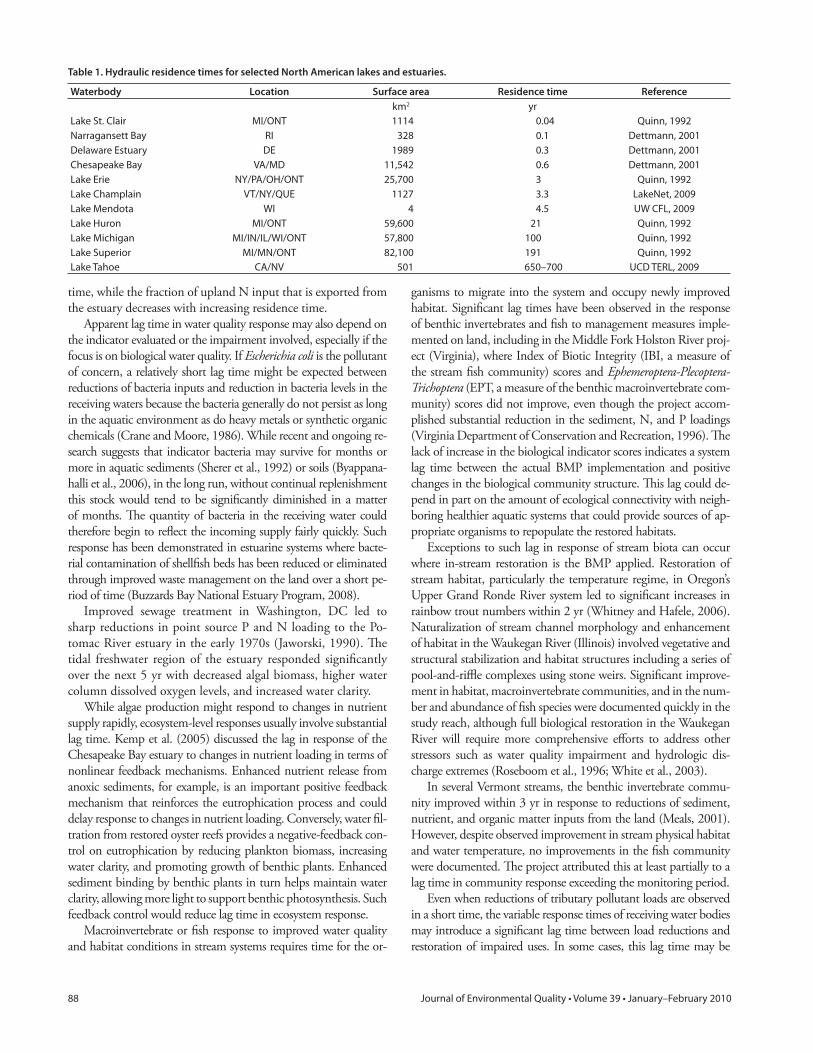
respond to changes in nutrient loading. Examples of residence

times for selected North American lakes and estuaries are shown

in Table 1. Simply on the basis of dilution, it will likely take

considerably longer for water column nutrient concentrations

to respond to a decrease in nutrient loading to Lake Superior

(residence time 191 yr) than to Lake St. Clair (residence time

0.04 yr). Beyond dilution alone, residence time infl uences how

a water body processes and exports nutrients. An analysis of an-

nual nutrient budgets for North Atlantic estuaries demonstrated

that the net fractional transport of N and P through estuaries to

the continental shelf is inversely correlated with the residence

time of water in the system (Nixon et al., 1996). Removal of N

by denitrifi cation and P loss by particulate settling were the pri-

mary processes responsible for removing nutrients, and the lon-

ger the water mass remains in the system, the greater the removal

of N and P. Similarly, Dettmann (2001) used modeling and data

from 11 North American and European estuaries to show that

the fraction of N denitrifi ed increases with increasing residence


time, while the fraction of upland N input that is exported from

the estuary decreases with increasing residence time.

Apparent lag time in water quality response may also depend on

the indicator evaluated or the impairment involved, especially if the

focus is on biological water quality. If Escherichia coli is the pollutant

of concern, a relatively short lag time might be expected between

reductions of bacteria inputs and reduction in bacteria levels in the

receiving waters because the bacteria generally do not persist as long

in the aquatic environment as do heavy metals or synthetic organic

chemicals (Crane and Moore, 1986). While recent and ongoing re-

search suggests that indicator bacteria may survive for months or

more in aquatic sediments (Sherer et al., 1992) or soils (Byappana-

halli et al., 2006), in the long run, without continual replenishment

this stock would tend to be signifi cantly diminished in a matter

of months. Th e quantity of bacteria in the receiving water could

therefore begin to refl ect the incoming supply fairly quickly. Such

response has been demonstrated in estuarine systems where bacte-

rial contamination of shellfi sh beds has been reduced or eliminated

through improved waste management on the land over a short pe-

riod of time (Buzzards Bay National Estuary Program, 2008).

Improved sewage treatment in Washington, DC led to

sharp reductions in point source P and N loading to the Po-

tomac River estuary in the early 1970s (Jaworski, 1990). Th e

tidal freshwater region of the estuary responded signifi cantly

over the next 5 yr with decreased algal biomass, higher water

column dissolved oxygen levels, and increased water clarity.

While algae production might respond to changes in nutrient

supply rapidly, ecosystem-level responses usually involve substantial

lag time. Kemp et al. (2005) discussed the lag in response of the

Chesapeake Bay estuary to changes in nutrient loading in terms of

nonlinear feedback mechanisms. Enhanced nutrient release from

anoxic sediments, for example, is an important positive feedback

mechanism that reinforces the eutrophication process and could

delay response to changes in nutrient loading. Conversely, water fi l-

tration from restored oyster reefs provides a negative-feedback con-

trol on eutrophication by reducing plankton biomass, increasing

water clarity, and promoting growth of benthic plants. Enhanced

sediment binding by benthic plants in turn helps maintain water

clarity, allowing more light to support benthic photosynthesis. Such

feedback control would reduce lag time in ecosystem response.

Macroinvertebrate or fi sh response to improved water quality

and habitat conditions in stream systems requires time for the or-

ganisms to migrate into the system and occupy newly improved

habitat. Signifi cant lag times have been observed in the response

of benthic invertebrates and fi sh to management measures imple-

mented on land, including in the Middle Fork Holston River proj-

ect (Virginia), where Index of Biotic Integrity (IBI, a measure of

the stream fi sh community) scores and Ephemeroptera-Plecoptera-Trichoptera (EPT, a measure of the benthic macroinvertebrate com-

munity) scores did not improve, even though the project accom-

plished substantial reduction in the sediment, N, and P loadings

(Virginia Department of Conservation and Recreation, 1996). Th e

lack of increase in the biological indicator scores indicates a system

lag time between the actual BMP implementation and positive

changes in the biological community structure. Th is lag could de-

pend in part on the amount of ecological connectivity with neigh-

boring healthier aquatic systems that could provide sources of ap-

propriate organisms to repopulate the restored habitats.

Exceptions to such lag in response of stream biota can occur

where in-stream restoration is the BMP applied. Restoration of

stream habitat, particularly the temperature regime, in Oregon’s

Upper Grand Ronde River system led to signifi cant increases in

rainbow trout numbers within 2 yr (Whitney and Hafele, 2006).

Naturalization of stream channel morphology and enhancement

of habitat in the Waukegan River (Illinois) involved vegetative and

structural stabilization and habitat structures including a series of

pool-and-riffl e complexes using stone weirs. Signifi cant improve-

ment in habitat, macroinvertebrate communities, and in the num-

ber and abundance of fi sh species were documented quickly in the

study reach, although full biological restoration in the Waukegan

River will require more comprehensive eff orts to address other

stressors such as water quality impairment and hydrologic dis-

charge extremes (Roseboom et al., 1996; White et al., 2003).

In several Vermont streams, the benthic invertebrate commu-

nity improved within 3 yr in response to reductions of sediment,

nutrient, and organic matter inputs from the land (Meals, 2001).

However, despite observed improvement in stream physical habitat

and water temperature, no improvements in the fi sh community

were documented. Th e project attributed this at least partially to a

lag time in community response exceeding the monitoring period.

Even when reductions of tributary pollutant loads are observed

in a short time, the variable response times of receiving water bodies

may introduce a signifi cant lag time between load reductions and

restoration of impaired uses. In some cases, this lag time may be

Table 1. Hydraulic residence times for selected North American lakes and estuaries.

Waterbody Location Surface area Residence time Reference

km2 yr

Lake St. Clair MI/ONT 1114 0.04 Quinn, 1992

Narragansett Bay RI 328 0.1 Dettmann, 2001

Delaware Estuary DE 1989 0.3 Dettmann, 2001

Chesapeake Bay VA/MD 11,542 0.6 Dettmann, 2001

Lake Erie NY/PA/OH/ONT 25,700 3 Quinn, 1992

Lake Champlain VT/NY/QUE 1127 3.3 LakeNet, 2009

Lake Mendota WI 4 4.5 UW CFL, 2009

Lake Huron MI/ONT 59,600 21 Quinn, 1992

Lake Michigan MI/IN/IL/WI/ONT 57,800 100 Quinn, 1992

Lake Superior MI/MN/ONT 82,100 191 Quinn, 1992

Lake Tahoe CA/NV 501 650–700 UCD TERL, 2009


relatively short. For example, researchers anticipate that the Ches-

apeake Bay could respond fairly rapidly to reductions in nutrient

loading, as incoming nutrients are quickly buried by sediment or

exported to the atmosphere or the ocean. Even beds of submerged

aquatic vegetation, critical to the Bay’s aquatic ecosystem, can return

within a few years after improvements in water clarity (Scientifi c and

Technical Advisory Committee Chesapeake Research Consortium,

2005). Bacteriological water quality in shellfi sh beds in Totten and

Eld Inlets (WA) estuaries improved rapidly in response to improved

animal waste management in the drainage area, but unfortunately

also deteriorated equally rapidly when animal waste management

practices on the land were abandoned (Spooner et al., 2008).

In contrast, lake response to changes in incoming P load is of-

ten delayed by recycling of P stored in aquatic sediments. When

P loads to Shagawa Lake (MN) were reduced by 80% through

tertiary wastewater treatment, residence time models predicted

new equilibrium P concentrations within 1.5 yr, but high in-lake

P levels continued to be maintained by recycling of P from lake

sediments (Larsen et al., 1979). Even more than 20 yr after the re-

duction of the external loading, sediment feedback of P continued

to infl uence the trophic state of the lake (Seo and Canale, 1999).

Similarly, St. Albans Bay (VT) in Lake Champlain failed to re-

spond rapidly to reductions in P load from its watershed. From 1980

through 1991, a combination of wastewater treatment upgrades

and intensive implementation of dairy waste management BMPs

through the Rural Clean Water Program (RCWP) brought about a

reduction of P loads to this eutrophic bay. However, water quality in

the bay did not improve signifi cantly; this pattern was attributed to

internal loading from sediments highly enriched in P from decades

of point and NPS inputs (Meals, 1992). Although researchers at

that time believed that the sediment P would begin to decline over

time as the internal supply was depleted, subsequent monitoring

has shown that P levels have not declined over the years as expected

(LCBP, 2008). Recent research has confi rmed that a substantial res-

ervoir of P continues to exist in the sediments that can be transferred

into the water under certain chemical conditions and nourish algae

blooms for many years to come (Druschel et al., 2005). In eff ect,

this internal loading has become a signifi cant source of P, one that

cannot be addressed by management measures on the land.

Eff ects Measurement Components of Lag Time

Watershed project managers are routinely pressed for results by a

wide range of stakeholders. Th e fundamental temporal components

of lag time control how long it will take for a response to occur, but

the eff ectiveness of measuring the response may cause a further delay

in recognizing it. It is possible for a response to occur unnoticed un-

less a suitable monitoring program is in place to detect it.

Th e magnitude of the potential eff ects produced by a water-

shed NPS management program depends on the eff ectiveness

of each unit of installed or adopted practices, the number of

practice units installed or adopted, the eff ectiveness with which

the practices are targeted to the correct pollutants and sources,

and numerous other factors. While not all responses can be

measured, the design of the monitoring program is a major

determinant of our ability to discern a response against the

background of the variability of natural systems.

In the context of lag time, sampling frequency with respect

to background variability is a key determinant of how long

it will take to document change. In a given system, taking n

samples per year provides a certain statistical power to detect a

trend. If the number of samples per year is reduced, statistical

power is reduced, and it may take longer to document a signifi -

cant trend or to state with confi dence that a concentration has

dropped below a water quality standard. Simply stated, taking

fewer samples a year is likely to introduce an additional “statis-

tical” lag time before a change can be eff ectively documented.

In an analysis of a monitoring program for the San Diego Coun-

ty (California) MS4 permit, Weston Solutions, Inc. (2005) assessed

the ability of a stormwater monitoring program to continue to de-

tect trends in receiving waters under diff erent sampling frequencies.

Th is analysis used existing data and projected trends into the future

using the slope of the current data set to predict when concentra-

tion of a constituent (based on a trend line from linear regression

against time) would drop below the water quality objective. An ex-

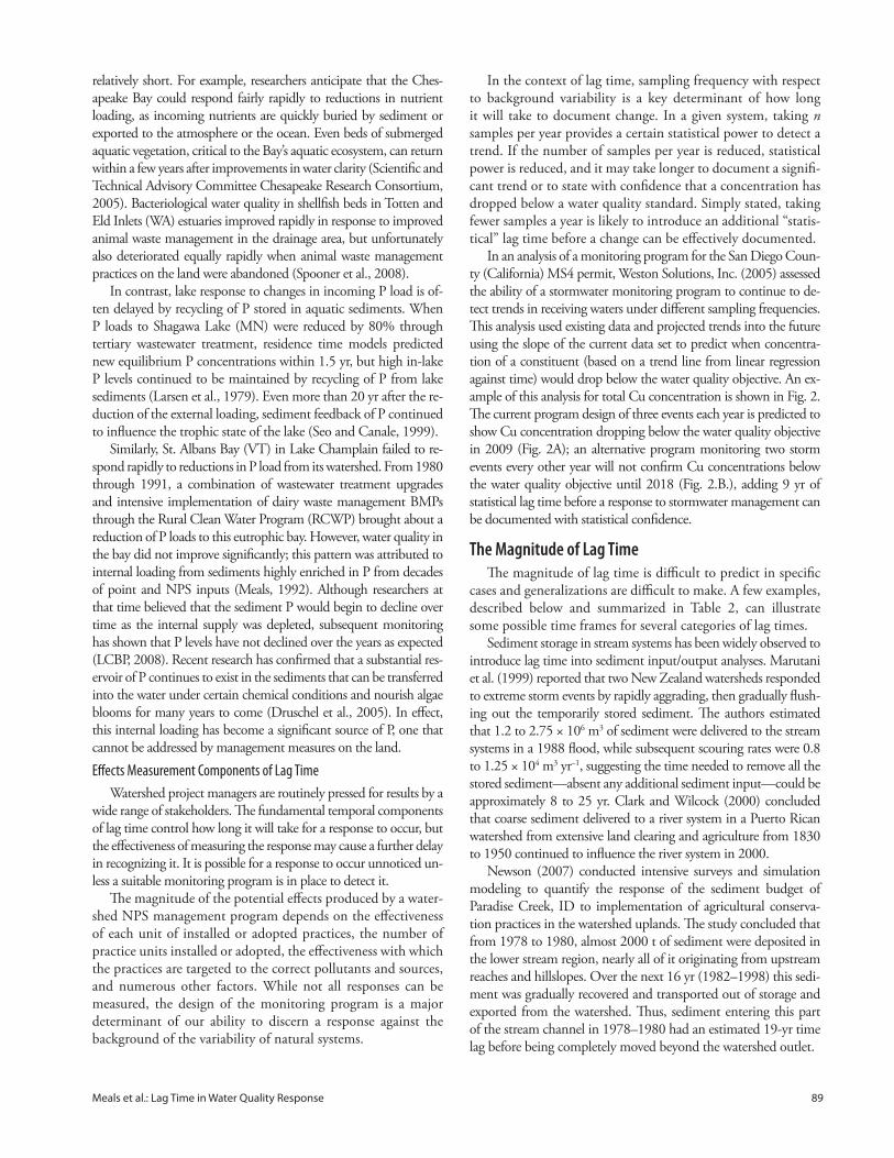
ample of this analysis for total Cu concentration is shown in Fig. 2.

Th e current program design of three events each year is predicted to

show Cu concentration dropping below the water quality objective

in 2009 (Fig. 2A); an alternative program monitoring two storm

events every other year will not confi rm Cu concentrations below

the water quality objective until 2018 (Fig. 2.B.), adding 9 yr of

statistical lag time before a response to stormwater management can

be documented with statistical confi dence.

The Magnitude of Lag TimeTh e magnitude of lag time is diffi cult to predict in specifi c

cases and generalizations are diffi cult to make. A few examples,

described below and summarized in Table 2, can illustrate

some possible time frames for several categories of lag times.

Sediment storage in stream systems has been widely observed to

introduce lag time into sediment input/output analyses. Marutani

et al. (1999) reported that two New Zealand watersheds responded

to extreme storm events by rapidly aggrading, then gradually fl ush-

ing out the temporarily stored sediment. Th e authors estimated

that 1.2 to 2.75 × 106 m3 of sediment were delivered to the stream

systems in a 1988 fl ood, while subsequent scouring rates were 0.8

to 1.25 × 104 m3 yr–1, suggesting the time needed to remove all the

stored sediment—absent any additional sediment input—could be

approximately 8 to 25 yr. Clark and Wilcock (2000) concluded

that coarse sediment delivered to a river system in a Puerto Rican

watershed from extensive land clearing and agriculture from 1830

to 1950 continued to infl uence the river system in 2000.

Newson (2007) conducted intensive surveys and simulation

modeling to quantify the response of the sediment budget of

Paradise Creek, ID to implementation of agricultural conserva-

tion practices in the watershed uplands. Th e study concluded that

from 1978 to 1980, almost 2000 t of sediment were deposited in

the lower stream region, nearly all of it originating from upstream

reaches and hillslopes. Over the next 16 yr (1982–1998) this sedi-

ment was gradually recovered and transported out of storage and

exported from the watershed. Th us, sediment entering this part

of the stream channel in 1978–1980 had an estimated 19-yr time

lag before being completely moved beyond the watershed outlet.


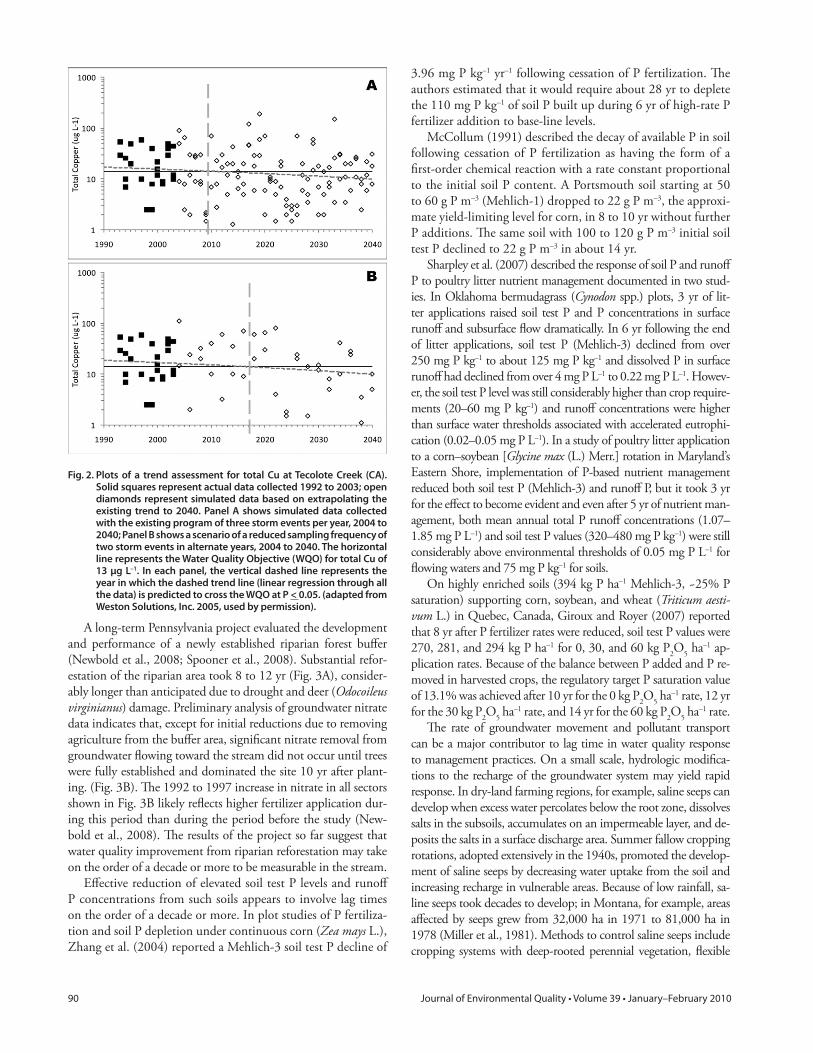
A long-term Pennsylvania project evaluated the development

and performance of a newly established riparian forest buff er

(Newbold et al., 2008; Spooner et al., 2008). Substantial refor-

estation of the riparian area took 8 to 12 yr (Fig. 3A), consider-

ably longer than anticipated due to drought and deer (Odocoileus virginianus) damage. Preliminary analysis of groundwater nitrate

data indicates that, except for initial reductions due to removing

agriculture from the buff er area, signifi cant nitrate removal from

groundwater fl owing toward the stream did not occur until trees

were fully established and dominated the site 10 yr after plant-

ing. (Fig. 3B). Th e 1992 to 1997 increase in nitrate in all sectors

shown in Fig. 3B likely refl ects higher fertilizer application dur-

ing this period than during the period before the study (New-

bold et al., 2008). Th e results of the project so far suggest that

water quality improvement from riparian reforestation may take

on the order of a decade or more to be measurable in the stream.

Eff ective reduction of elevated soil test P levels and runoff

P concentrations from such soils appears to involve lag times

on the order of a decade or more. In plot studies of P fertiliza-

tion and soil P depletion under continuous corn (Zea mays L.),

Zhang et al. (2004) reported a Mehlich-3 soil test P decline of

3.96 mg P kg–1 yr–1 following cessation of P fertilization. Th e

authors estimated that it would require about 28 yr to deplete

the 110 mg P kg–1 of soil P built up during 6 yr of high-rate P

fertilizer addition to base-line levels.

McCollum (1991) described the decay of available P in soil

following cessation of P fertilization as having the form of a

fi rst-order chemical reaction with a rate constant proportional

to the initial soil P content. A Portsmouth soil starting at 50

to 60 g P m–3 (Mehlich-1) dropped to 22 g P m–3, the approxi-

mate yield-limiting level for corn, in 8 to 10 yr without further

P additions. Th e same soil with 100 to 120 g P m–3 initial soil

test P declined to 22 g P m–3 in about 14 yr.

Sharpley et al. (2007) described the response of soil P and runoff

P to poultry litter nutrient management documented in two stud-

ies. In Oklahoma bermudagrass (Cynodon spp.) plots, 3 yr of lit-

ter applications raised soil test P and P concentrations in surface

runoff and subsurface fl ow dramatically. In 6 yr following the end

of litter applications, soil test P (Mehlich-3) declined from over

250 mg P kg–1 to about 125 mg P kg–1 and dissolved P in surface

runoff had declined from over 4 mg P L–1 to 0.22 mg P L–1. Howev-

er, the soil test P level was still considerably higher than crop require-

ments (20–60 mg P kg–1) and runoff concentrations were higher

than surface water thresholds associated with accelerated eutrophi-

cation (0.02–0.05 mg P L–1). In a study of poultry litter application

to a corn–soybean [Glycine max (L.) Merr.] rotation in Maryland’s

Eastern Shore, implementation of P-based nutrient management

reduced both soil test P (Mehlich-3) and runoff P, but it took 3 yr

for the eff ect to become evident and even after 5 yr of nutrient man-

agement, both mean annual total P runoff concentrations (1.07–

1.85 mg P L–1) and soil test P values (320–480 mg P kg–1) were still

considerably above environmental thresholds of 0.05 mg P L–1 for

fl owing waters and 75 mg P kg–1 for soils.

On highly enriched soils (394 kg P ha–1 Mehlich-3, ~25% P

saturation) supporting corn, soybean, and wheat (Triticum aesti-vum L.) in Quebec, Canada, Giroux and Royer (2007) reported

that 8 yr after P fertilizer rates were reduced, soil test P values were

270, 281, and 294 kg P ha–1 for 0, 30, and 60 kg P2O

5 ha–1 ap-

plication rates. Because of the balance between P added and P re-

moved in harvested crops, the regulatory target P saturation value

of 13.1% was achieved after 10 yr for the 0 kg P2O

5 ha–1 rate, 12 yr

for the 30 kg P2O

5 ha–1 rate, and 14 yr for the 60 kg P

2O

5 ha–1 rate.

Th e rate of groundwater movement and pollutant transport

can be a major contributor to lag time in water quality response

to management practices. On a small scale, hydrologic modifi ca-

tions to the recharge of the groundwater system may yield rapid

response. In dry-land farming regions, for example, saline seeps can

develop when excess water percolates below the root zone, dissolves

salts in the subsoils, accumulates on an impermeable layer, and de-

posits the salts in a surface discharge area. Summer fallow cropping

rotations, adopted extensively in the 1940s, promoted the develop-

ment of saline seeps by decreasing water uptake from the soil and

increasing recharge in vulnerable areas. Because of low rainfall, sa-

line seeps took decades to develop; in Montana, for example, areas

aff ected by seeps grew from 32,000 ha in 1971 to 81,000 ha in

1978 (Miller et al., 1981). Methods to control saline seeps include

cropping systems with deep-rooted perennial vegetation, fl exible

Fig. 2. Plots of a trend assessment for total Cu at Tecolote Creek (CA). Solid squares represent actual data collected 1992 to 2003; open diamonds represent simulated data based on extrapolating the existing trend to 2040. Panel A shows simulated data collected with the existing program of three storm events per year, 2004 to 2040; Panel B shows a scenario of a reduced sampling frequency of two storm events in alternate years, 2004 to 2040. The horizontal line represents the Water Quality Objective (WQO) for total Cu of 13 μg L–1. In each panel, the vertical dashed line represents the year in which the dashed trend line (linear regression through all the data) is predicted to cross the WQO at P < 0.05. (adapted from Weston Solutions, Inc. 2005, used by permission).


crop rotations, and surface drainage of upland recharge areas to re-

duce the amount of water percolating through the root zone. In

Montana, hydrologic controls, including planting of alfalfa (Medi-cago sativa L.) dropped the water table up to 200 cm and eff ectively

dried out the subsoil, reducing hydraulic pressures from the re-

charge to the discharge areas, eliminating saline discharge in < 5 yr

(Halvorson and Reule, 1980; Miller et al., 1981).

While groundwater levels may respond relatively quickly to

changes in vegetation, transport of solutes in groundwater can take

considerably longer, especially as the size of the system increas-

es. For example, Delaware’s Inland Bays, comprising a 77-km2

estuary on the state’s southern Atlantic coast, suff er from excessive

nutrient and sediment loading, resulting in degraded communi-

ties of benthic organisms, submerged vegetation, and fi sh. Nitrate

delivered to the Bays in groundwater discharge from agricultural

fi elds and poultry operations and from septic-system effl uent in

the 830-km2 watershed is one of the most severe stressors of the

Inland Bays. Studies and eff orts to reduce nitrate loading have

been underway for two decades, from state, university, and USGS

groundwater studies in the 1970s to a USDA Hydrologic Unit

Area (HUA) project in the 1990s to a total maximum daily load

(TMDL) in 2004. Unfortunately, estuary response to restoration

eff orts is constrained by the estimated 50 yr required for ground-

water to travel from agricultural land in the watershed to the Bays

(Bratton et al., 2004; Krantz et al., 2004).

In the Pequea and Mill Creek Watershed (Pennsylvania) Clean

Water Act Section 319 National Nonpoint Source Monitoring

Program (NNPSMP) Project (1994–2003), changes in fertilizer

applications to cropland in a 3.6 km2 watershed did not result in

reductions in stream N concentrations due to lag time between

applications and nutrients reaching stream channel. Groundwa-

ter age dating conducted during the study indicated that N ap-

plied to land reached springs in 2 to 3 yr, but groundwater fl ow to

the stream channel took 15 to 39 yr (Galeone, 2005).

Tomer and Burkart (2003) presented extensive evidence

from two ~30 ha Iowa agricultural watersheds that at least

several decades were required for subsurface water to travel

from the watershed divide to the stream and concluded that,

in many watersheds, changes in agricultural practices may take

several decades to fully eff ect changes in groundwater quality.

In their study watersheds, for example, groundwater concen-

trations of NO3–N in 2003 were still infl uenced by heavy N

fertilizer applications that occurred in the 1970s.

Researchers in the Walnut Creek Restoration (Iowa)

NNPSMP Project (1995–2005) conducted a groundwater

travel time analysis using a geographic information system

(GIS) and readily available soil and topographic data to evalu-

ate the time needed to observe changes in stream nitrate N

concentrations resulting from conversion of row crop land to

native prairie (Schilling and Wolter, 2007). Mean groundwa-

ter travel time in the 7.8 km2 watershed was estimated to be

10.1 yr, with a range from 2 d to 308 yr. Researchers estimated

that 10 to 22% of restored prairie areas contributed groundwa-

ter to streams in the Walnut Creek watershed within the 10-yr

Table 2. Examples of lag times reported in response to environmental impact or treatment.

Parameter(s) Scale Impact/Treatment Response lag Reference

Sediment Large watershed Extreme storm events 8–25 yr Marutani et al., 1999

Sediment River basin Land clearing/agriculture > 50 yr Clark and Wilcock, 2000

Sediment Large watershed Cropland erosion control 19 yr Newson, 2007

Chloride Large aquifer Road salt > 50 yr Bester et al., 2006

Salinity Field Hydrologic control/alfalfa cropping 5 yr Halvorson and Reule, 1980 Miller et al., 1981

NO3–N Small watersheds N fertilizer rates > 30 yr Tomer and Burkart, 2003

NO3–N River basin N fertilizer rates > 50 yr Bratton et al., 2004

NO3–N Large watersheds Nutrient management ≥ 5 yr STAC, 2005

NO3–N Small watershed Nutrient management 15–39 yr Galeone, 2005

NO3–N Small watershed Prairie restoration 10 yr Schilling and Spooner, 2006

NO3–N Small watershed Riparian forest buff er 10 yr Newbold et al., 2008

NO3–N Small watersheds N fertilizer rates 4–10 yr Owens et al., 2008

Soil test P Field P fertilizer rates 8–14 yr McCollum, 1991

Soil test P Plot P fertilizer rates 28 yr Zhang et al., 2004

Soil test P Field P fertilizer rates 10–14 yr Giroux and Royer, 2007

Soil and runoff P Plot/fi eld Poultry litter management > 5 yr Sharpley et al., 2007

P Lake WWTP upgrade > 20 yr Larsen et al., 1979

P Lake WWTP upgrade/agricultural BMPs > 20 yr LCBP, 2008

P, N, E. coli Small watersheds Livestock exclusion ≤ 1 yr Meals, 2001

Fecal bacteria Estuary Waste management < 1 yr BBNEP, 2008

Fecal bacteria Estuary Waste management 1 yr Spooner et al., 2008

Algal biomass, dissolved oxygen, water clarity

Estuary Wastewater treatment < 5 yr Jaworski, 1995

Macroinvertebrates Small watersheds Livestock exclusion 3 yr Meals, 2001

Macroinvertebrates Small watersheds Mine waste treatment 10 yr Chadwick et al., 1986

Fish fi rst order stream Habitat restoration 2 yr Whitney and Hafele, 2006

Fish Large watershed Conservation Reserve Program (before/after) 25 yr Marshall et al., 2008

Fish Small watershed Acid mine drainage treatment 3–9 yr Cravotta, 2009


project period. Despite this relatively small contribution, the

project was able to document signifi cant reductions in stream

nitrate concentrations in response to prairie restoration (Schil-

ling and Spooner, 2006) and researchers anticipate additional

nitrate reduction as reduced-nitrate groundwater from addi-

tional watershed area reaches the stream network.

Owens et al. (2008) reported that groundwater quality re-

sponse to changes in N fertilization rate took several years to

observe even in very small (< 2 ha) watersheds. When N appli-

cation rate was increased from 56 to 168 kg ha–1 yr–1, NO3–N

concentrations in groundwater and streamfl ow took 4 yr to

respond, and then continued to increase for 10 yr. After N ad-

ditions were discontinued, NO3–N in groundwater discharge

did not return to pre-treatment levels for 6 yr. Even where clay

layers forced groundwater discharge pathways to be very shal-

low, suggesting a potentially rapid response to changes in N

inputs, the lag in groundwater NO3–N concentration response

to management changes was still 3 yr or more.

Research in the Chesapeake Bay Watershed has emphasized the

likelihood of a substantial lag time between implementation of

BMPs and reductions in N loading to the Bay (Phillips and Lind-

sey, 2003; Scientifi c and Technical Advisory Committee Chesa-

peake Research Consortium, 2005). Groundwater supplies a sig-

nifi cant amount of water and N to streams in the watershed and

about half of the N load in streams in the Bay watershed is thought

to be transported through groundwater. Th e age of groundwater

in shallow aquifers in the Chesapeake Bay watershed ranges from

<1 to more than 50 yr. Th e median age of all samples was 10 yr,

with 25% of the samples having an age of 7 yr or less and 75%

of the samples having an age of up to 13 yr. Based on this age as

representative of time of travel, scientists estimated that in a sce-

nario of complete elimination of N applications in the watershed,

a 50% reduction in base fl ow nitrate concentrations would take

about 5 yr, with equilibrium reached in about 2040.

Bester et al. (2006) studied the impact of road salt on a mu-

nicipal wellfi eld outside Toronto, ON, using monitoring data

and numerical simulation. Th eir results suggested that the aqui-

fer system contains a large and heterogeneously distributed mass

of chloride and that some of the wells may not yet have reached

their maximum chloride concentrations even after 57 yr (1945–

2002) of road salt application. Conversely, the simulations indi-

cated that although the system responds rapidly to reductions in

salt loading, the residual chloride mass may take decades to fl ush

out, even if road salting were discontinued. Under conditions of

continuous salt input, attainment of equilibrium concentrations

in the system may require on the order of 100 yr.

In sum, at best only broad ranges of lag times can be gener-

alized. In the Chesapeake Bay watershed, where lag time issues

have been examined closely, Phillips and Lindsey (2003) pro-

posed some general guidelines for considering lag times in the

Bay restoration program (Table 3).

DiscussionSeveral important factors aff ect lag time. Scale is clearly an im-

portant infl uence; intuitively, response to BMPs should be more

rapid at small scales than in larger settings. Th e relationship between

scale and response, however, does not appear to be consistent (see

Table 2). Note that lag time for soil test P response to change in P

fertilizer rate was 28 yr in a plot study (Zhang et al., 2004); while

lag time for P, N, and E. coli response to livestock exclusion in small

watersheds was 1 yr or less (Meals, 2001). Physical processes, such

as sediment transport in streams, aff ect the rate at which response

to a perturbation or a management improvement is delivered to a

water body. Chemical processes, such as sorption kinetics in soils or

aquatic sediments, have often delayed expected responses to changes

in pollutant loading. Groundwater movement frequently controls

the rate at which changes in pollutant loads are delivered to receiv-

ing surface waters. Th e type of management, including selection

of appropriate BMPs, application of BMPs to critical source areas,

and achievement of a suffi ciently high level of treatment to eff ect

change, will aff ect the nature and speed of response in water quality.

Selection of an indicator and the design of the monitoring system

help determine how and when a water quality response to changes

in land management can be detected.

In most situations, some lag time between implementation

of BMPs and water quality response is inevitable. Although the

exact duration of the lag can rarely be predicted, in many cases

the lag time will exceed the length of typical monitoring periods,

Fig. 3. A. Plot of changes in basal area of trees in Zone 2 of a planted riparian forest buff er system in Pennsylvania, 1992 to 2007. B. Plot of mean annual nitrate concentrations in groundwater and stream water in the riparian forest buff er system, 1992 to 2007. “Field” refers to the corn fi eld draining to the buff er, “Zones 1 and 2” are the forested areas closest to the stream, and “Zone 3” refers to the herbaceous or grass fi lter strip between the forested zone and the upland fi eld. Standard deviations for individual points averaged 1.35 (range: 0.41–2.0) mg L–1 for groundwater and 0.61 (range: 0.25 to 1.2) mg L–1 for stream water. Sample sizes ranged from 15 to 28 per year (adapted from Newbold et al. 2008, used by permission).


making it problematic to document a water quality response. Sev-

eral possible approaches are proposed to deal with this challenge.

Recognize Lag time and Adjust ExpectationsIt usually takes time for a water body to become impaired

and it will take time to accomplish the clean-up. However,

once a water quality problem is recognized and action is taken,

the public and political system usually expect quick results.

Failure to meet such expectations may cause frustration, pes-

simism, and a reluctance to pursue further action. It is up to

scientists, investigators, and project managers to do a better

job explaining to all stakeholders in realistic terms that current

water quality impairments usually result from historically poor

land management and that immediate solutions should not be

expected. For example, a 2005 report (Scientifi c and Techni-

cal Advisory Committee Chesapeake Research Consortium,

2005) advised the Chesapeake Bay Program to better commu-

nicate the implications of the lag time between management

actions, watershed properties, and cycles in weather conditions

on the restoration of the Chesapeake Bay, noting that eff ective

communication of this point will be very important for con-

tinued support of eff orts to implement BMPs even though the

results of these actions often will not be immediately observed.

Characterize the WatershedBefore designing a NPS management program and an as-

sociated monitoring program, investigate important watershed

characteristics likely to infl uence lag time. Determining the time

of travel for groundwater movement is an obvious example. Wa-

tershed characterization is an important step in the project plan-

ning process (USEPA, 2005) and such characterization should

especially address important aspects of the hydrologic and geo-

logic setting, as well as documentation of NPS pollution sources

and the nature of the water quality impairment, all of which can

infl uence observed lag time in system response.

Consider Lag Time Issues in Selection, Siting,

and Monitoring of Best Management PracticesFirst and foremost, proper BMP selection must be based on

solving the problem and ensuring that landowners have the ca-

pability and willingness to implement and maintain the BMPs.

Lag time can, however, be an important factor in the fi nal design

of BMP systems, ensuring, for example, that when down-gradi-

ent BMPs are installed, they are ready to handle the anticipated

runoff or pollutant load from up-gradient sources. In addition

to that, when projects include targeted BMP monitoring to

document interim water quality improvements, recognition of

lag time may require an adjustment of the approach to target-

ing the management program. When designing a program for

projects that include BMP-specifi c monitoring, potential BMPs

should be evaluated to determine which practices might provide

the most rapid improvement in water quality, given watershed

characteristics. For example, practices aff ecting direct delivery of

nutrients into surface runoff and streamfl ow, such as barnyard

runoff management, may yield more rapid reductions in nutrient

loading to the receiving water than practices that reduce nutri-

ent leaching to groundwater, when groundwater time of travel is

measured in years. Fencing livestock out of streams may give im-

mediate water quality improvement, compared to waiting for ri-

parian forest buff ers to grow. Such considerations, combined with

application of other criteria such as cost eff ectiveness, can help

determine priorities for BMP programs in a watershed project.

Lag time should also be considered in locating management

practices within a watershed. Managers should consider the need

to demonstrate results to the public, which may be easier at small

scales, along with the need to achieve water quality targets and

consequent wider benefi ts at the large watershed scale. Where

sediment and sediment-bound pollutants from cropland erosion

are primary concerns, for example, implementing practices that

target the largest sediment sources closest to the receiving wa-

ter may provide a more rapid water quality benefi t than erosion

controls in the upper reaches of the watershed. Where ground-

water transport is a key determinant of response, application of

a groundwater travel time model such as that used in Walnut

Creek, Iowa (Schilling and Wolter, 2007) before application of

management changes could at least help managers understand

when to anticipate water quality response and communicate this

issue to the public, or at best support targeting of an initial round

of application of management measures to land areas where the

eff ects are expected to be transmitted to receiving waters quickly.

It is important to point out that factoring lag time into BMP

selection and targeting is not to say that long-term management

improvements like riparian forest buff er restoration should be

discounted or that upland sediment sources should be ignored.

Rather, it is suggested that planners and managers may want to

Table 3. Guidelines for considering lag times in the Chesapeake Bay restoration program (Phillips and Lindsey, 2003).

Nutrient sourceManagement practice implementation time Watershed residence time Implications for load reductions to Chesapeake Bay

Point sources Several years Hours to weeks Would provide most rapid improvement of water quality due to immediate reduction of source.

Dissolved nutrients from nonpoint sources

Several years Hours to months if associated with runoff /soil water

Years to decades if associated with groundwater (median time 10 yr)

Once fully treatments fully implemented, there would be a fairly rapid reduction of loads associated with runoff and

soil water. Nitrogen loads associated with groundwater would have a median time of 10 yr for water quality

improvements to be evident.

Sediment-associated nutrients from nonpoint sources

Several years Decades or longer, depending on location in watershed

Load reductions would be greatly infl uenced by streamfl ow variability. Storm events would deliver

sediment and associated nutrients contained on land and in stream corridors to the Bay may not show reductions

for decades due to long residence times.


consider implementing BMPs and treating sources likely to ex-

hibit short lag times fi rst to increase the probability of demon-

strating some water quality improvement as quickly as possible.

“Quick-fi x” practices with minimum lag time should not au-

tomatically replace practices implemented in locations that can

ultimately yield permanent reductions in pollutant loads.

Monitor Small Watersheds Close to SourcesIn cases where documentation of the eff ects of a manage-

ment program on water quality is a critical goal, lag time can

sometimes be minimized by focusing monitoring on small wa-

tersheds, close to pollution sources. Lag times introduced by

transport phenomena (e.g., groundwater travel, sediment fl ux

through stream networks) will likely be shorter in small water-

sheds than in larger basins. In the extreme, this principle im-

plies monitoring at the edge of fi eld or above/below a limited

treated area, but small watersheds (e.g., < 1500 ha) can also

yield good results. In the NNPSMP, projects monitoring BMP

programs in small watersheds (e.g., the Morro Bay Watershed

Project in California, the Jordan Cove Project in Connecticut,

the Pequea/Mill Creek Watershed Project in Pennsylvania, and

the Lake Champlain Basin Watersheds Project in Vermont)

were more successful in documenting improvements in water

quality in response to change than were projects that took place

in large watersheds (e.g., the Lightwood Knot Creek Project in

Alabama and the Sny Magill Watershed Project in Iowa) in the

7 to 10 yr time frame of the NNPSMP (Spooner et al., 2008).

Monitoring programs can be designed to get a better handle

on lag time issues. Monitoring indicators at all points along the

pathway from source to response or conducting periodic syn-

optic surveys over the course of a project will identify changes

as they occur and document progress toward the end response.

Special studies of sediment transport, soil P levels, groundwa-

ter dynamics, or receiving water behavior can shed light on

phenomena that aff ect lag time in water quality response. For

example, the Long Creek Watershed (NC) NNPSMP Project

(1993–2002) conducted special studies of the eff ects of a wet-

land on PAH concentrations in an urban stream, the use of mi-

crobial indicators to assess land use impacts, and interactions

between P and stream sediments to better explain the temporal

and spatial water quality response to a BMP program (Line

and Jennings, 2002). Supplementing a stream monitoring

program with special studies can help project managers under-

stand watershed processes, predict potential lag times, and help

explain delays in water quality improvement to stakeholders.

In the Walnut Creek (Iowa) watershed, no changes in stream

suspended sediment loads were documented, despite extensive

conversion of row crop land to prairie and reductions in fi eld

erosion predicted by RUSLE; a 22-mile stream survey revealed

that streambank erosion contributed more than 50% of Wal-

nut Creek sediment export (Spooner et al., 2008).

Select Indicators CarefullySome water quality variables can be expected to change more

quickly than others in response to management changes. For ex-

ample, Tomer and Burkart (2003) recommended that shallow

monitoring of unsaturated-zone waters, rather than in-stream

monitoring, may be the most reliable means to document the ef-

fects of changes in crop rotations and fertilization on water qual-

ity. As documented in the Jordan Cove (CT) NNPSMP Project

(1996–2005), peak storm fl ows from a developing watershed can

be reduced quickly through application of stormwater infi ltration

practices (Clausen, 2004). Reductions in nutrient loads in sur-

face waters might be expected to occur promptly in response to a

ban on winter application of animal waste in northern states. Th e

NNPSMP projects in California, North Carolina, Pennsylvania,

and Vermont (Spooner et al., 2008) demonstrated rapid reduc-

tions in nutrients and bacteria by reducing direct deposition of

livestock waste in surface waters through fencing livestock out of

streams. However, improvements in stream biota appear to come

much more slowly, beyond the time frame of many monitoring

eff orts. Where restoration of biological integrity is a goal, this may

argue for a more sustained monitoring eff ort to document a bio-

logical response to land treatment. Failing that, however, selection

of indicators that have relatively short lag times where possible will

make it easier (and quicker) to demonstrate success.

Incorporate Lag Time into Simulation ModelingIn long-term restoration eff orts in complex systems, simula-

tion models are often used for program planning, forecasting,

and evaluation. However, most current models do not handle

the lag time issue well; signifi cant improvements are needed

before models can represent actual landscape processes to pro-

vide more realistic predictions of water quality changes.

Design Monitoring Programs to Detect Change Eff ectivelyMonitor at locations and at a frequency suffi cient to detect

change with reasonable sensitivity. Assess background variability

before the project begins and conduct a minimum detectable

change analysis (Spooner et al., 1987; Richards and Grabow,

2003) to determine a sampling frequency suffi cient to document

the anticipated magnitude of change with statistical confi dence.

Although lag time will still be a factor in actual system response,

a paired-watershed design (Clausen and Spooner, 1993; King

et al., 2008), where data from an untreated watershed are used

to control for weather and other sources of variability, is one of

the most eff ective ways to document water quality changes in

response to improvements in land management. If a monitoring

program is intended to detect trends, evaluate statistical power to

determine the best sampling frequency for the project.

Target monitoring to the eff ects expected from the BMPs im-

plemented, in the sequence that those eff ects are anticipated. For

example, when the ultimate goal is habitat/biota restoration in an

urban stream, if BMPs are implemented fi rst that will alter peak

stormfl ows, design the monitoring program to track changes in hy-

drology. After the needed hydrologic restoration is achieved, moni-

toring can be redirected to track expected changes in channel mor-

phology. Once changes in channel morphology are documented,

monitoring can then focus on assessment of habitat and biological

community response. Response of stream hydrology is likely to be

quicker than restoration of stream biota and would therefore be a

valuable—and more prompt—indicator of progress.


ConclusionsLag time between implementation of management practices

on the land and water quality response is an unfortunate fact of

life in watershed management. Unless recognized and dealt with,

long lag time will frequently confound our ability to successfully

document improved water quality resulting from treatment of

NPS and may discourage vital restoration eff orts. While ongoing

and future research may provide us with better tools to predict

and account for lag time, it is essential that watershed monitor-

ing programs today recognize and grapple with this issue. Useful

approaches to deal with the inevitable lag between implementa-

tion of management practices and water quality response include

educating stakeholders on reasonable expectations, appropriately

characterizing the watershed and pollutant delivery processes; con-

sidering lag time in selection, siting, and monitoring of manage-

ment measures; selection of appropriate indicators with which to

assess progress; and designing eff ective monitoring programs to

detect water quality response and document eff ectiveness.

ReferencesBester, M.L., E.O. Frind, J.W. Molson, and D.L. Rudolph. 2006. Numerical

investigation of road salt impact on an urban wellfi eld. Ground Water 44:165–175.

Bratton, J.F., J.K. Böhlke, F.M. Manheim, and D.E. Krantz. 2004. Submarine ground water in Delmarva Peninsula coastal bays: Ages and nutrients. Ground Water 42:1021–1034.

Buzzards Bay National Estuary Program. 2008. Turning the tide on shellfi sh bed closures in Buzzards Bay during the 1990s. Available at http://www.buzzardsbay.org/shellclssuccess.htm (verifi ed 19 Oct. 2009).

Byappanahalli, M.N., R.L. Whitman, D.A. Shively, M.J. Sadowsky, and S. Ishii. 2006. Population structure, persistence, and seasonality of autochthonous Escherichia coli in temperate, coastal forest soil from a Great Lakes watershed. Environ. Microbiol. 8:504–513.

Chadwick, J.W., S.P. Canton, and R.L. Dent. 1986. Recovery of benthic invertebrate communities in Silver Bow Creek, Montana following improved metal mine wastewater treatment. Water Air Soil Pollut. 28:427–438.

Clark, J.J., and P.R. Wilcock. 2000. Eff ects of Land-use change on channel morphology in northeastern Puerto Rico. Geol. Soc. Am. Bull. 112:1763–1777.

Clausen, J.C. 2004. Jordan Cover Urban Watershed Section 319 National Monitoring Program Project. Annual Report. College of Agriculture and Natural Resources, Univ. of Connecticut, Storrs.

Clausen, J.C., and J. Spooner. 1993. Paired watershed study design. USEPA Publ. 841-F-93–009. U.S. Environ. Protection Agency, Washington, DC.

Crane, S.R., and J.A. Moore. 1986. Modeling enteric bacterial die-off : A review. Water Air Soil Pollut. 27:411–439.

Cravotta, C.A., III. 2009. Abandoned mine drainage in the Swatara Creek Basin, Southern Anthracite Coalfi eld, Pennsylvania, USA: 1. Streamwater-quality trends coinciding with the return of fi sh. Mine Water Environ. (in press).

Dettmann, E.H. 2001. Eff ect of water residence time on annual export and denitrifi cation of nitrogen in estuaries: A model analysis. Estuaries 24:481–490.

Druschel, G., A. Hartmann, R. Lomonaco, and K. Oldrid. 2005. Determination of sediment phosphorus concentrations in St. Albans Bay, Lake Champlain: Assessment of internal loading and seasonal variations of phosphorus sediment-water column cycling. Final Report prepared for Vermont Agency of Natural Resources, Dep. of Geology, Univ. of Vermont, Burlington.

Gale, J.A., D.E. Line, D.L. Osmond, S.W. Coff ey, J. Spooner, J.A. Arnold, T.J. Hoban, and R.C. Wimberly. 1993. Evaluation of the experimental rural clean water program. EPA-841-R-93–005. Natl. Water Quality Evaluation Project, NCSU Water Quality Group, Biological and Agric. Engineering Dep., North Carolina State Univ., Raleigh.

Galeone, D.G. 2005. Pequea and Mill Creek Watersheds Section 319 NMP Project: Eff ects of Streambank Fencing on Surface-water Quality. NWQEP Notes 118: August, 2005. North Carolina State Univ., Raleigh.

Giroux, M., and R. Royer. 2007. Long term eff ects of phosphate applications on yields, evolution of P soil test, saturation, and solubility in two very rich soils. Agrosolutions 18:17–24. Inst. de recherche et de développement en agroenvironnement (IRDA), Québec, Canada. (In French, with English abstract.)

Goodman, J., J.M. Collins, and K.B. Rapp. 1992. Nitrate and pesticide occurrence in shallow groundwater during the Oakwood Lakes-Poinsett RCWP project. p. 33–45. In Th e National Rural Clean Water Program Symp., September 1992. Orlando, FL. ORD EPA/625/R-92/006. USEPA, Washington, DC.

Gunsalus, B., E.G. Flaig, and G. Ritter. 1992. Eff ectiveness of agricultural best management practices implemented in the Taylor Creek/Nubbin Slough Watershed and the Lower Kissimmee River Basin. p. 161–171. In Th e National Rural Clean Water Program Symp., September 1992. Orlando, FL. ORD EPA/625/R-92/006. USEPA, Washington, DC.

Halvorson, A.D., and C.A. Reule. 1980. Alfalfa for hydrologic control of saline seeps. Soil Sci. Soc. Am. J. 44:370–374.

Jaworski, N. 1990. Retrospective of the water quality issues of the upper Potomac estuary. Aquat. Sci. 3:11–40.

Jokela, W.E., J.C. Clausen, D.W. Meals, and A.N. Sharpley. 2004. Eff ectiveness of agricultural best management practices in reducing phosphorus loading to Lake Champlain. p. 39–52. In T. Manley et al. (ed.) Lake Champlain: Partnership and research in the new millennium. Kluwer Academic/Plenum Publ., New York.

Kemp, W.M., W.R. Boynton, J.E. Adolf, D.F. Boesch, W.C. Boicourt, G. Brush, J.C. Cornwell, T.R. Fisher, P.M. Glibert, J.D. Hagy, L.W. Harding, E.D. Houde, D.G. Kimmel, W.D. Miller, R.I.E. Newell, M.R. Roman, E.M. Smith, and J.C. Stevenson. 2005. Eutrophication of Chesapeake Bay: Historical trends and ecological interactions. Mar. Ecol. Prog. Ser. 303:1–29.

King, K.W., P.C. Smiley, Jr., B.J. Baker, and N.R. Fausey. 2008. Validation of paired watersheds for assessing conservation practices in the Upper Big Walnut Creek watershed, Ohio. J. Soil Water Conserv. 63:380–395.

Koerkle, E.H. 1992. Eff ects of nutrient management on surface water quality in a small watershed in Pennsylvania. p. 193–207. In Th e National Rural Clean Water Program Symposium, September 1992. Orlando, FL. ORD EPA/625/R-92/006. USEPA, Washington, DC.

Krantz, D.E., F.T. Manheim, J.F. Bratton, and D.J. Phelan. 2004. Hydrogeologic setting and ground-water fl ow beneath a section of Indian River Bay, Delaware. Ground Water 42:1035–1051.

Lafl en, J.M., R. Lal, and S.A. El-Swaify. 1990. Soil erosion and a sustainable agricultura. p. 569–581. In C.A. Edwards et al. (ed.) Sustainable agriculture systems. Soil and Water Conserv. Soc., Ankeny, IA.

Lake Champlain Basin Program. 2008. State of the lake and ecosystem indicators report—2008. Available at http://www.lcbp.org/PDFs/SOL2008-web.pdf (verifi ed 19 Oct. 2009). Lake Champlain Basin Program, Grand Isle, VT.

LakeNet. 2009. Lake profi le: Champlain. Available at http://www.worldlakes.org/lakedetails.asp?lakeid = 8518 (verifi ed 19 Oct. 2009). LakeNet Secretariat, Annapolis, MD.

Larsen, D.P., J. Van Sickle, K.W. Malueg, and P.D. Smith. 1979. Th e eff ect of wastewater phosphorus removal on Shagawa Lake, Minnesota: Phosphorus supplies, lake phosphorus, and chlorophyll a. Water Res. 13:1259–1272.

Line, D.E., and G.D. Jennings. 2002. Long Creek watershed nonpoint source water quality monitoring project–Final report. North Carolina State Univ., Raleigh.

Marshall, D.W., A.H. Fayram, J.C. Panuska, J. Baumann, and J. Hennessey. 2008. Positive eff ects of agricultural land use changes on coldwater fi sh communities in Southwest Wisconsin streams. N. Am. J. Fish. Manage. 28:944–953.

Marutani, T., M. Kasai, L.M. Reid, and N.A. Trustrum. 1999. Infl uence of storm-related sediment storage on the sediment delivery from tributary catchments in the Upper Waipaoa River, New Zealand. Earth Surf. Processes Landforms 24:881–896.

McCollum, R.E. 1991. Buildup and decline of soil phosphorus: 30-Year trends on a Typic Umprabuult. Agron. J. 83:77–85.

Meals, D.W. 1992. Water quality trends in the St. Albans Bay, Vermont watershed following RCWP land treatment. p. 47–58. In Th e National Rural Clean Water Program Symp., September 1992. Orlando, FL. ORD EPA/625/R-92/006. USEPA, Washington, DC.

Meals, D.W. 1993. Assessing nonpoint source phosphorus control in the LaPlatte River watershed. Lake Reservoir Manage. 7:197–207.

Meals, D.W. 1996. Watershed-scale response to agricultural diff use pollution control programs in Vermont, USA. Water Sci. Technol. 33:197–204.


Meals, D.W. 2001. Water quality response to riparian restoration in an agricultural watershed in Vermont, USA. Water Sci. Technol. 43:175–182.

Miller, H.R., P.L. Brown, J.J. Donovan, R.N. Bergatino, J.L. Sondregger, and F.A. Schmidt. 1981. Saline seep development and control in the North American Great Plains—Hydrogeological aspects. Agric. Water Manage. 4:115–141.

Newbold, J.D., J.W. Elwood, R.V. O’Neil, and W. Van Winkle. 1981. Measuring nutrient spiralling in streams. Can. J. Fish. Aquat. Sci. 38:860–863.

Newbold, J.D., S. Herbert, B.W. Sweeney, and P. Kiry. 2008. Water quality functions of a 15-year-old riparian forest buff er system. p. 1–7. In Riparian ecosystems and buff ers: Working at the water’s edge. AWRA Summer Specialty Conf. Am. Water Resources Assoc., Virginia Beach, VA.

Newson, J. 2007. Measurement and modeling of sediment transport in a northern Idaho stream. Masters thesis. Biological and Agric. Eng., College of Graduate Studies, Univ. of Idaho, Moscow.

Nixon, S.W., J.W. Ammerman, L.P. Atkinson, V.M. Berounsky, G. Billen, W.C. Boicourt, W.R. Boynton, T.M. Church, D.M. Ditoro, R. Elmgren, J.H. Garber, A.E. Giblin, R.A. Jahnke, N.J.P. Owens, M.E.Q. Pilson, and S.P. Seitzinger. 1996. Th e fate of nitrogen and phosphorus at the land-sea margin of the North Atlantic Ocean. Biogeochemistry 35:141–180.

Owens, L.B., M.J. Shipitalo, and J.V. Bonta. 2008. Water quality response times to pasture management changes in small and large watersheds. J. Soil Water Conserv. 63:292–299.

Phillips, S.W., and B.D. Lindsey. 2003. Th e infl uence of ground water on nitrogen delivery to the Chesapeake Bay. USGS Fact Sheet FS-091–03. Available at http://md.water.usgs.gov/publications/fs-091–03/index.html (verifi ed 19 Oct. 2009). U.S. Geological Surv., MD-DE-DC Water Sci. Ctr., Baltimore, MD.

Pote, D.H., T.C. Daniel, A.N. Sharpley, P.A. Moore, D.R. Edwards, and D.J. Nichols. 1996. Relating extractable soil phosphorus to phosphorus losses in runoff . Soil Sci. Soc. Am. J. 60:855–859.

Quinn, F.H. 1992. Hydraulic residence times for the Laurentian Great Lakes. J. Great Lakes Res. 18:22–28.

Rao, P.S.C., A.G. Hornsby, and R.E. Jessup. 1985. Indices for ranking the potential for pesticide contamination of groundwater. Proc. Soil Crop Sci. Soc. Fla. 44:1–8.

Richards, R.P., and G.L. Grabow. 2003. Detecting reductions in sediment loads associated with Ohio’s conservation reserve enhancement program. J. Am. Water Resour. Assoc. 39:1261–1268.

Roseboom, D.P., T.E. Hill, J. Beardsley, J.A. Rodsater, and L. Duong. 1996. Waukegan River National Monitoring Program, biological and physical monitoring of Waukegan River restoration eff orts in biotechnical bank protection and pool/riffl e creation, 1996. ISWS CR-629:1998 Illinois State Water Survey, Champaign.

Schilling, K.E., and J. Spooner. 2006. Eff ects of watershed-scale land use change on stream nitrate concentrations. J. Environ. Qual. 35:2132–2145.

Schilling, K.E., and C.F. Wolter. 2007. A GIS-based groundwater travel time model to evaluate stream nitrate concentration reductions from land use change. Environ. Geol. 53:433–443.

Scientifi c and Technical Advisory Committee, Chesapeake Bay Program. 2005. Understanding “lag times” aff ecting the improvement of water quality in the Chesapeake Bay. STAC Publ. 05–001. Available at http://www.chesapeake.org/stac/Pubs/LagTimeReport.pdf (verifi ed 19 Oct. 2009). Chesapeake Bay Program, Edgewater, MD.

Seo, D., and R.P. Canale. 1999. Analysis of sediment characteristics and total phosphorus models for Shagawa Lake. J. Environ. Eng. 125:346–350.

Sharpley, A.N., S. Herron, and T. Daniel. 2007. Overcoming the challenges of phosphorus-based management in poultry farming. J. Soil Water Conserv. 62:375–389.

Sherer, B.M., J.R. Miner, J.A. Moore, and J.C. Buckhouse. 1992. Indicator bacterial survival in stream sediments. J. Environ. Qual. 21:591–595.

Sims, J.T., A.C. Edwards, O.F. Schoumans, and R.R. Simard. 2000. Integrating soil phosphorus testing into environmentally based agricultural management practices. J. Environ. Qual. 29:60–71.

Spooner, J., C.J. Jamieson, R.P. Maas, and M.D. Smolen. 1987. Determining statistically signifi cant changes in water quality pollutant concentrations. Lake Reservoir Manage. 3:195–201.

Spooner, J., L.A. Szpir, D.E. Line, D.L. Osmond, D.W. Meals, and G.L. Grabow. 2008. 2008 Summary Report: Section 319 National Monitoring Program Projects, National Nonpoint Source Watershed Project Studies, NCSU Water Quality Group, Biological and Agricultural Engineering Dep., North Carolina State Univ., Raleigh.

Tomer, M.D., and M.R. Burkart. 2003. Long-term eff ects of nitrogen fertilizer use on ground water nitrate in two small watersheds. J. Environ. Qual. 32:2158–2171.

USEPA. 2005. Handbook for developing watershed plans to restore and protect our waters. EPA 841-B-05–005. U.S. Environmental Protection Agency, Offi ce of Water, Washington, DC.

Virginia Department of Conservation and Recreation. 1996. Alternative watering systems for livestock-Th e Middle Fork Holston River builds on success. Available at http://www.epa.gov/owow/NPS/Section319II/VA.html (verifi ed 19 Oct. 2009). USEPA Offi ce of Wetlands, Oceans, and Watersheds, Washington, DC.

Wang, D., S.N. Levine, D.W. Meals, J.P. Hoff mann, J.C. Drake, and E.A. Cassell. 1999. Importance of in-stream nutrient storage to phosphorus export from a rural, eutrophic river in Vermont, USA. p. 205–223. In T.O. Manley and P.L. Manley (ed.) Lake Champlain in transition: From research toward restoration. Water Science and Application, Vol. 1, American Geophysical Union, Washington, DC.

Weston Solutions, Inc. 2005. Monitoring program recommendations for report of waste discharge. Report prepared for San Diego County Copermittees, County of San Diego, Watershed Protection, Dep. of Public Works. Available at http://www.westonsolutions.com/services/environmental_solutions/water_resources/index.htm (verifi ed 19 Oct. 2009). Weston Solutions, Inc., Carlsbad, CA.

White, W.P., J. Beardsley, J.A. Rodsater, L. Duong, and T.E. Hill. 2003. Biological and physical monitoring of Waukegan River restoration eff orts in biotechnical bank protection and pool/riffl e creation: Annual data report, May 31, 2003. Illinois Environ. Protection Agency, Springfi eld, IL.

Whitney, L., and R. Hafele. 2006. Stream restoration and fi sh in Oregon’s Upper Grand Ronde river system. NWQEP Notes. Available at http://www.bae.ncsu.edu/programs/extension/wqg/issues/notes123.pdf (verifi ed 19 Oct. 2009). North Carolina State Univ. Coop. Ext., Raleigh.

Zhang, T.Q., A.F. MacKenzie, B.C. Liang, and C.F. Drury. 2004. Soil test phosphorus and phosphorus fractions with long-term phosphorus addition and depletion. Soil Sci. Soc. Am. J. 68:519–528.

lag time in water quality response to best management ... time in water quality... · expectations...

Documents