lagrangian and hamiltonian structure of complex …marsden/wiki/uploads/oberwolfach/... ·...

LAGRANGIAN AND HAMILTONIAN

STRUCTURE OF

COMPLEX FLUIDS

Tudor S. Ratiu

Section de Mathematiques and Bernoulli Center

Ecole Polytechnique Federale de Lausanne, Switzerland

[email protected]

Joint work with Francois Gay-Balmaz

To appear in Advances in Applied Mathematics

Oberwolfach, July 2008

1

PLAN OF THE PRESENTATION

• Affine Lagrangian and Hamiltonian reduction

• Example 1: Ericksen-Leslie equations

• Example 2: Eringen equations

PUNCHLINE: All these equations are obtained by Euler-Poincareand Lie-Poisson reduction from material representation. These re-duction procedures need to be extended to include affine terms andthe groups have a relatively complicated internal structure adaptedto complex fluids.


2

AFFINE LAGRANGIAN ANDHAMILTONIAN REDUCTION

ρ : G→ Aut(V ) right representation, S = GsV ; multiplication is

(g1, v1)(g2, v2) = (g1g2, v2 + ρg2(v1)).

The Lie alebra s = gsV of S has bracket

ad(ξ1,v1)(ξ2, v2) = [(ξ1, v1), (ξ2, v2)] = ([ξ1, ξ2], v1ξ2 − v2ξ1),

where vξ denotes the induced action of g on V , that is,

vξ :=d

dt

∣∣∣∣t=0

ρexp(tξ)(v) ∈ V.

If (ξ, v) ∈ s and (µ, a) ∈ s∗ we have

ad∗(ξ,v)(µ, a) = (ad∗ξ µ+ v a, aξ),where aξ ∈ V ∗ and v a ∈ g∗ are given by

aξ :=d

dt

∣∣∣∣t=0

ρ∗exp(−tξ)(a) and 〈v a, ξ〉g := −〈aξ, v〉V ,

〈·, ·〉g : g∗ × g→ R and 〈·, ·〉V : V ∗ × V → R are the duality parings.Oberwolfach, July 2008

3

Lagrangian semidirect product theory

• L : TG× V ∗ → R which is right G-invariant.

• So, if a0 ∈ V ∗, define the Lagrangian La0 : TG→ R by La0(vg) :=L(vg, a0). Then La0 is right invariant under the lift to TG of theright action of Ga0 on G, where Ga0 := g ∈ G | ρ∗ga0 = a0.

• Right G-invariance of L permits us to define l : g× V ∗ → R by

l(TgRg−1(vg), ρ∗g(a0)) = L(vg, a0).

• For a curve g(t) ∈ G, let ξ(t) := TRg(t)−1(g(t)) and define thecurve a(t) as the unique solution of the following linear differ-ential equation with time dependent coefficients

a(t) = −a(t)ξ(t),

with initial condition a(0) = a0. Solution is a(t) = ρ∗g(t)(a0).


4

i With a0 held fixed, Hamilton’s variational principle

δ∫ t2t1La0(g(t), g(t))dt = 0,

holds, for variations δg(t) of g(t) vanishing at the endpoints.

ii g(t) satisfies the Euler-Lagrange equations for La0 on G.

iii The constrained variational principle

δ∫ t2t1l(ξ(t), a(t))dt = 0,

holds on g× V ∗, upon using variations (δξ, δa) of the form

δξ =∂η

∂t− [ξ, η], δa = −aη,

where η(t) ∈ g vanishes at the endpoints.

iv The Euler-Poincare equations hold on g× V ∗:∂

∂t

δl

δξ= − ad∗ξ

δl

δξ+δl

δa a.


5

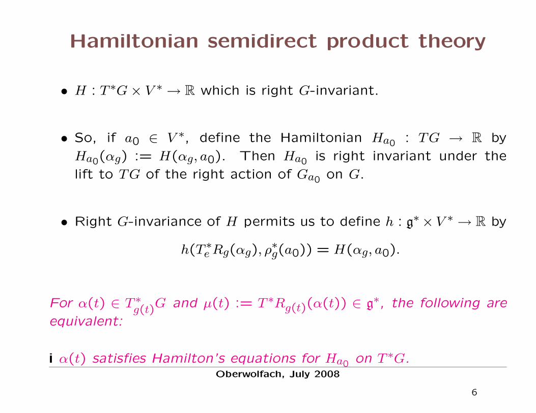
Hamiltonian semidirect product theory

• H : T ∗G× V ∗ → R which is right G-invariant.

• So, if a0 ∈ V ∗, define the Hamiltonian Ha0 : TG → R by

Ha0(αg) := H(αg, a0). Then Ha0 is right invariant under the

lift to TG of the right action of Ga0 on G.

• Right G-invariance of H permits us to define h : g∗× V ∗ → R by

h(T ∗eRg(αg), ρ∗g(a0)) = H(αg, a0).

For α(t) ∈ T ∗g(t)G and µ(t) := T ∗Rg(t)(α(t)) ∈ g∗, the following are

equivalent:

i α(t) satisfies Hamilton’s equations for Ha0 on T ∗G.Oberwolfach, July 2008

6

ii The Lie-Poisson equation holds on s∗:

∂

∂t(µ, a) = − ad∗(

δhδµ,

δhδa

)(µ, a) = −(

ad∗δhδµ

µ+δh

δa a, a

δh

δµ

), a(0) = a0

where s is the semidirect product Lie algebra s = gsV . The asso-ciated Poisson bracket is the Lie-Poisson bracket on the semidirectproduct Lie algebra s∗, that is,

f, g(µ, a) =

⟨µ,

[δf

δµ,δg

δµ

]⟩+

⟨a,δf

δa

δg

δµ−δg

δa

δf

δµ

⟩.

As on the Lagrangian side, the evolution of the advected quantitiesis given by a(t) = ρ∗

g(t)(a0).

Legendre transformation: h(µ, a) := 〈µ, ξ〉 − l(ξ, a), where µ = δlδξ. If

it is invertible, since

δh

δµ= ξ and

δh

δa= −

δl

δa,

the Lie-Poisson equations for h are equivalent to the Euler-Poincareequations for l together with the advection equation a+ aξ = 0.


7

Affine Lagrangian semidirect product theory

Let c ∈ F(G,V ∗) be a right one-cocycle, that is, it verifies the

property c(fg) = ρ∗g−1(c(f)) + c(g) for all f, g ∈ V ∗. This implies

that c(e) = 0 and c(g−1) = −ρ∗g(c(g)). Instead of the contragredient

representation ρ∗g−1 of G on V ∗ form the affine right representation

θg(a) = ρ∗g−1(a) + c(g).

Note thatd

dt

∣∣∣∣t=0

θexp(tξ)(a) = aξ + dc(ξ).

and

〈aξ + dc(ξ), v〉V = 〈dcT (v)− v a, ξ〉g,

where dc : g→ V ∗ is defined by dc(ξ) := Tec(ξ), and dcT : V → g∗ is

defined by

〈dcT (v), ξ〉g := 〈dc(ξ), v〉V .


8

• L : TG × V ∗ → R right G-invariant under the affine action(vh, a) 7→ (ThRg(vh), θg(a)) = (ThRg(vh), ρ∗

g−1(a) + c(g)).

• So, if a0 ∈ V ∗, define La0 : TG → R by La0(vg) := L(vg, a0).Then La0 is right invariant under the lift to TG of the rightaction of Gca0

on G, where Gca0:= g ∈ G | θg(a0) = a0.

• Right G-invariance of L permits us to define l : g× V ∗ → R by

l(TgRg−1(vg), θg−1(a0)) = L(vg, a0).

• For a curve g(t) ∈ G, let ξ(t) := TRg(t)−1(g(t)) and define thecurve a(t) as the unique solution of the following affine differ-ential equation with time dependent coefficients

a(t) = −a(t)ξ(t)− dc(ξ(t)),

with initial condition a(0) = a0. The solution can be written asa(t) = θg(t)−1(a0).


9

i With a0 held fixed, Hamilton’s variational principle

δ∫ t2t1La0(g(t), g(t))dt = 0,

holds, for variations δg(t) of g(t) vanishing at the endpoints.

ii g(t) satisfies the Euler-Lagrange equations for La0 on G.

iii The constrained variational principle

δ∫ t2t1l(ξ(t), a(t))dt = 0,

holds on g× V ∗, upon using variations of the form

δξ =∂η

∂t− [ξ, η], δa = −aη − dc(η),

where η(t) ∈ g vanishes at the endpoints.

iv The affine Euler-Poincare equations hold on g× V ∗:∂

∂t

δl

δξ= −ad∗ξ

δl

δξ+δl

δa a− dcT

(δl

δa

).


10

Lagrangian Approach to Continuum Theories

of Perfect Complex Fluids

Two key observations:

1. Enlarge the configuration manifold Diff(D) to a bigger group G

that contains variables in the Lie group O of order parameters.

2. The usual advection equations (for the mass density, the entropy,

the magnetic field, etc) need to be augmented by a new advected

quantity on which the group G acts by an affine representation.

O the order parameter Lie group, F(D,O) := χ : D → O smooth

Basic idea for complex fluids: enlarge the “particle relabeling group”

Diff(D) to the semidirect product G = Diff(D)sF(D,O).


11

Diff(D) acts on F(D,O) via the right action

(η, χ) ∈ Diff(D)×F(D,O) 7→ χ η ∈ F(D,O).

Therefore, the group multiplication is given by

(η, χ)(ϕ,ψ) = (η ϕ, (χ ϕ)ψ).

Fix a volume form µ on D, so identify densities with functions, one-

form densitities with one-forms, etc. But the dual actions will be

of course different once these identifications are used.

The Lie algebra g of the semidirect product group is

g = X(D)sF(D, o),

and the Lie bracket is computed to be

ad(u,ν)(v, ζ) = (adu v, adν ζ + dν · v − dζ · u),

where adu v = −[u,v], adν ζ ∈ F(D, o) is given by adν ζ(x) :=

adν(x) ζ(x), and dν ·v ∈ F(D, o) is given by dν ·v(x) := dν(x)(v(x)).Oberwolfach, July 2008

12

g∗ = Ω1(D)sF(D, o∗)

through the pairing

〈(m, κ), (u, ν)〉 =∫D

(m · u + κ · ν)µ.

The dual map to ad(u,ν) is

ad∗(u,ν)(m, κ) =(£um + (div u)m + κ · dν, ad∗ν κ+ div(uκ)

).

Explanation of the symbols:

• κ · dν ∈ Ω1(D) denotes the one-form defined by

κ · dν(vx) := κ(x)(dν(vx))

• ad∗ν κ ∈ F(D, o∗) denotes the o∗-valued mapping defined by

ad∗ν κ(x) := ad∗ν(x)(κ(x)).

• uκ is the 1-contravariant tensor field with values in o∗ defined by

uκ(αx) := αx(u(x))κ(x) ∈ o∗.Oberwolfach, July 2008

13

So uκ is a generalization of the notion of a vector field. X(D, o∗)denotes the space of all o∗-valued 1-contravariant tensor fields.

• div(u) denotes the divergence of the vector field u with respect to

the fixed volume form µ. Recall that it is defined by the condition

(div u)µ = £uµ.

This operator can be naturally extended to the space X(D, o∗) as

follows. For w ∈ X(D, o∗) we write w = waεa where (εa) is a basis

of o∗ and wa ∈ X(D). We define div : X(D, o∗)→ F(D, o∗) by

divw := (divwa)εa.

Note that if w = uκ we have

div(uκ) = dκ · u + (div u)κ.

Split the space of advected quantities in two: usual ones and new

ones that involve affine actions and cocycles.Oberwolfach, July 2008

14

Affine representation space: V ∗1 ⊕V∗

2 , V ∗i are subspaces of the space

of all tensor fields on D, possibly with values in a vector space.

• V ∗1 is only acted upon by the component Diff(D) of G.

• The action of G on V ∗2 is affine, with the restriction that the affine

term only depends on the second component F(D,O) of G.

• Right affine representation of G = Diff(D)sF(D,O) on V ∗1 ⊕ V∗

2 :

(a, γ) ∈ V ∗1 ⊕ V∗

2 7→ (aη, γ(η, χ) + C(χ)) ∈ V ∗1 ⊕ V∗

2 ,

where γ(η, χ) denotes the representation of (η, χ) ∈ G on γ ∈ V ∗2 ,

and C ∈ F(F(D,O), V ∗2 ) satisfies the cocycle identity

C((χ ϕ)ψ) = C(χ)(ϕ,ψ) + C(ψ).

The representation ρ and the affine term c in the general theory are

ρ∗(η,χ)−1(a, γ) = (aη, γ(η, χ)) and c(η, χ) = (0, C(χ)).


15

• The infinitesimal action of (u, ν) ∈ g on γ ∈ V ∗2 is:

γ(u, ν) = γu + γν.

• The diamond operation: for (v, w) ∈ V1 ⊕ V2 we have

(v, w) (a, γ) = (v a+ w 1 γ,w 2 γ),

where 1 and 2 are associated to the induced representations ofthe first and second component of G on V ∗2 . On the right hand side, is associated to the representation of Diff(D) on V ∗1 . Usually, V ∗1is naturally the dual of some space V1 of tensor fields on D. Forexample the (p, q) tensor fields are naturally in duality with the (q, p)tensor fields. For a ∈ V ∗1 and v ∈ V1, the duality pairing is given by

〈a, v〉 =∫D

(a · v)µ,

where · denotes the contraction of tensor fields.

• The affine cocycle is c(η, χ) = (0, C(χ)). Hence

dcT (v, w) = (0,dCT (w)).


16

• For a Lagrangian l = l(u, ν, a, γ) : [X(D)sF(D, o)]s [V ∗1⊕V∗

2 ]→ R,

the affine Euler-Poincare equations become∂

∂t

δl

δu= −£u

δl

δu− (div u)

δl

δu−δl

δν· dν +

δl

δa a+

δl

δγ1 γ

∂

∂t

δl

δν= − ad∗ν

δl

δν− div

(uδl

δν

)+

δl

δγ2 γ − dCT

(δl

δγ

),

and the advection equations area+ au = 0γ + γu + γν + dC(ν) = 0.


17

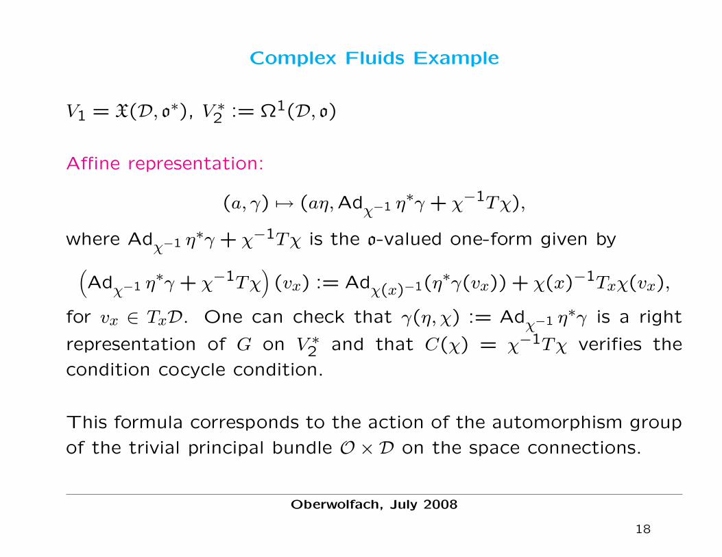
Complex Fluids Example

V1 = X(D, o∗), V ∗2 := Ω1(D, o)

Affine representation:

(a, γ) 7→ (aη,Adχ−1 η∗γ + χ−1Tχ),

where Adχ−1 η∗γ + χ−1Tχ is the o-valued one-form given by(Adχ−1 η

∗γ + χ−1Tχ)

(vx) := Adχ(x)−1(η∗γ(vx)) + χ(x)−1Txχ(vx),

for vx ∈ TxD. One can check that γ(η, χ) := Adχ−1 η∗γ is a right

representation of G on V ∗2 and that C(χ) = χ−1Tχ verifies the

condition cocycle condition.

This formula corresponds to the action of the automorphism group

of the trivial principal bundle O ×D on the space connections.


18

For this example we have

γu = £uγ, γν = − adν γ and dC(ν) = dν,

where adν γ ∈ Ω1(M, o) and dν ∈ Ω1(D, o) are the one-forms

(adν γ) (vx) := adν(x)(γ(vx)) = [ν(x), γ(vx)], dν(vx) := Txν(vx) ∈ o.

A direct computation shows that

w 1 γ = (divw) · γ − w · i dγ ∈ Ω1(D),

w 2 γ = −Tr(ad∗γ w) ∈ F(D, o∗),dCT (w) = −divw ∈ F(D, o∗),

where Tr denotes the trace of the o∗-valued (1,1) tensor

ad∗γ w : T ∗D × TD → o∗, (αx, vx) 7→ ad∗γ(vx)(w(αx)).

In coordinates we have Tr(ad∗γ w) = ad∗γiwi.


19

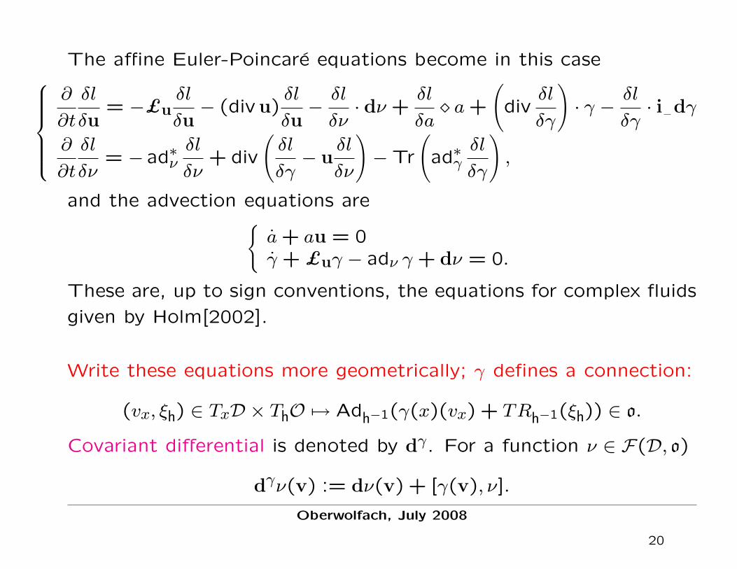
The affine Euler-Poincare equations become in this case∂

∂t

δl

δu= −£u

δl

δu− (div u)

δl

δu−δl

δν· dν +

δl

δa a+

(div

δl

δγ

)· γ −

δl

δγ· i dγ

∂

∂t

δl

δν= − ad∗ν

δl

δν+ div

(δl

δγ− u

δl

δν

)−Tr

(ad∗γ

δl

δγ

),

and the advection equations area+ au = 0γ + £uγ − adν γ + dν = 0.

These are, up to sign conventions, the equations for complex fluids

given by Holm[2002].

Write these equations more geometrically; γ defines a connection:

(vx, ξh) ∈ TxD × ThO 7→ Adh−1(γ(x)(vx) + TRh−1(ξh)) ∈ o.

Covariant differential is denoted by dγ. For a function ν ∈ F(D, o)

dγν(v) := dν(v) + [γ(v), ν].


20

The covariant divergence of w ∈ X(D, o∗) is the function

divγ w := divw −Tr(ad∗γ w) ∈ F(D, o∗),defined as minus the adjoint of the covariant differential, that is,∫

D(dγν · w)µ = −

∫D

(ν · divγ w)µ

for all ν ∈ F(D, o).

Note that the Lie derivative of γ ∈ Ω1(D, o) can be written as

£uγ(v) = d(γ(u))(v) + iudγ(v)

= dγ(γ(u))(v)− [γ(v), γ(u)] + dγγ(u,v)− [γ(u), γ(v)]

= dγ(γ(u))(v) + iuB(v),

where

B := dγγ = dγ + [γ, γ],

is the curvature of the connection induced by γ.

Note also that, using covariant differentiation, we have

w 1 γ = (divw) · γ − w · i dγ = (divγ w) · γ − w · i B.Oberwolfach, July 2008

21

Therefore, in terms of dγ,divγ, and B = dγγ, the equations read∂

∂t

δl

δu= −£u

δl

δu− (div u)

δl

δu−δl

δν· dν +

δl

δa a+

(divγ

δl

δγ

)· γ −

δl

δγ· i B

∂

∂t

δl

δν= − ad∗ν

δl

δν− div

(uδl

δν

)+ divγ

δl

δγ,

and a+ au = 0γ + dγ(γ(u)) + iuB + dγν = 0.

The Curvature Representation

Want to reformulate the reduction process and the equations of

motion in terms of (u, ν, a, B), instead of (u, ν, a, γ), where B =

dγγ = dγ + [γ, γ] ∈ Ω2(D, o) is the curvature of γ. With this choice

of variables the action of G becomes linear instead of affine. We

shall also assume that the Lagrangian L, and hence also l, depend

on γ only through B. We shall use therefore standard Euler-Poincare

reduction for semidirect products.Oberwolfach, July 2008

22

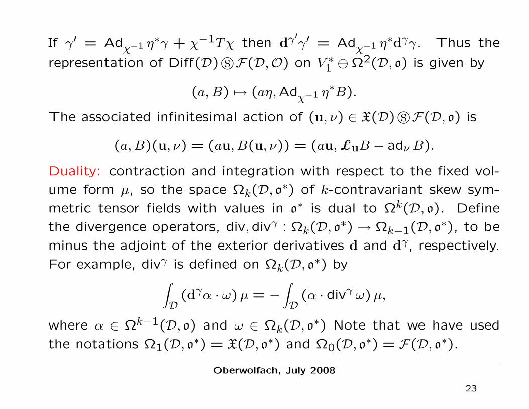
If γ′ = Adχ−1 η∗γ + χ−1Tχ then dγ′γ′ = Adχ−1 η∗dγγ. Thus the

representation of Diff(D)sF(D,O) on V ∗1 ⊕Ω2(D, o) is given by

(a,B) 7→ (aη,Adχ−1 η∗B).

The associated infinitesimal action of (u, ν) ∈ X(D)sF(D, o) is

(a,B)(u, ν) = (au, B(u, ν)) = (au,£uB − adν B).

Duality: contraction and integration with respect to the fixed vol-

ume form µ, so the space Ωk(D, o∗) of k-contravariant skew sym-

metric tensor fields with values in o∗ is dual to Ωk(D, o). Define

the divergence operators, div,divγ : Ωk(D, o∗)→ Ωk−1(D, o∗), to be

minus the adjoint of the exterior derivatives d and dγ, respectively.

For example, divγ is defined on Ωk(D, o∗) by∫D

(dγα · ω)µ = −∫D

(α · divγ ω)µ,

where α ∈ Ωk−1(D, o) and ω ∈ Ωk(D, o∗) Note that we have used

the notations Ω1(D, o∗) = X(D, o∗) and Ω0(D, o∗) = F(D, o∗).


23

If (v, b) ∈ V1 ⊕ Ω2(D, o∗) and (a,B) ∈ V ∗1 ⊕ Ω2(D, o), then

(v, b) (a,B) = (v a+ b 1 B, b 2 B),

where

b 1 B = (div b) · i B − b · i dB ∈ Ω1(D)

b 2 B = −Tr(ad∗B b) = − ad∗Bij bij ∈ F(D, o∗).

The (usual semidirect product) Euler-Poincare equation are

∂

∂t

δl

δu= −£u

δl

δu− (div u)

δl

δu−δl

δν· dν +

δl

δa a

+(

divδl

δB

)· i B −

δl

δB· i dB

∂

∂t

δl

δν= − ad∗ν

δl

δν+

δl

δB2 B −Tr

(ad∗B

δl

δB

),

and the advection equations area+ au = 0B + £uB − adν B = 0.

The affine EP equations imply these standard EP equations.Oberwolfach, July 2008

24

Affine Hamiltonian semidirect product theory

RT∗

g is the lift of right translation on G: RT∗

g (αf) = T ∗Rg−1(αf).

Let C : G×G→ T ∗G be a smooth map such that Cg(f) := C(g, f) ∈T ∗fgG, for all f, g ∈ G and define Ψg : T ∗G→ T ∗G by

Ψg(αf) := RT∗

g (αf) + Cg(f),

where C : G×G→ T ∗G satisfies Cg(f) ∈ T ∗fgG, for all f, g ∈ G.

The following are equivalent.

i Ψg is a right action.

ii For all f, g, h ∈ G, the affine term C verifies the property

Cgh(f) = Ch(fg) +RT∗

h (Cg(f)).

iii There exists α ∈ Ω1(G) such that Cg(f) = α(fg)−RT ∗g (α(f)).Oberwolfach, July 2008

25

The one-form α is unique if we assume that α(e) = 0, which is what

we will do from now on. Let Ω10(G) := α ∈ Ω1(G) | α(e) = 0 and

C(G) = C : G×G→ T ∗G | Cgh(f) = Ch(fg) +RT∗

h (Cg(f)), ∀f, g, h ∈G.

Let G act on (T ∗G,Ωcan) by the right affine action

Ψg(βf) := RT∗

g (βf) + Cg(f),

where C ∈ C(G). Let α ∈ Ω10(G) be the one-form associated to C.

i tα : βq ∈ (T ∗G,Ωcan) 7→ βq −α(q) ∈ (T ∗G,Ωcan− π∗Gdα) symplectic.

The action induced by Ψg on (T ∗G,Ωcan−π∗Gdα) through tα is RT∗

g .

ii Suppose that dα is G-invariant. Then the action Ψg is symplectic

relative to the canonical symplectic form Ωcan.


26

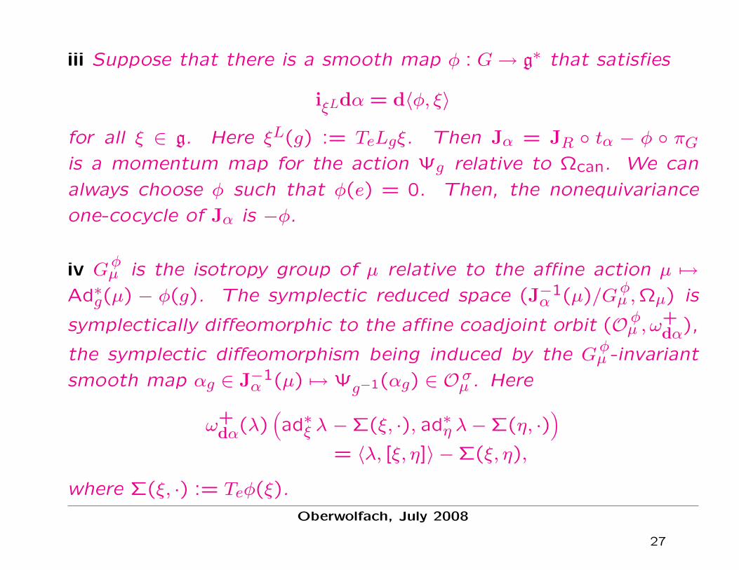
iii Suppose that there is a smooth map φ : G→ g∗ that satisfies

iξLdα = d〈φ, ξ〉

for all ξ ∈ g. Here ξL(g) := TeLgξ. Then Jα = JR tα − φ πGis a momentum map for the action Ψg relative to Ωcan. We can

always choose φ such that φ(e) = 0. Then, the nonequivariance

one-cocycle of Jα is −φ.

iv Gφµ is the isotropy group of µ relative to the affine action µ 7→

Ad∗g(µ) − φ(g). The symplectic reduced space (J−1α (µ)/Gφ

µ ,Ωµ) is

symplectically diffeomorphic to the affine coadjoint orbit (O φµ , ω

+dα),

the symplectic diffeomorphism being induced by the Gφµ -invariant

smooth map αg ∈ J−1α (µ) 7→ Ψg−1(αg) ∈ O σ

µ . Here

ω+dα(λ)

(ad∗ξ λ −Σ(ξ, ·), ad∗η λ−Σ(η, ·)

)= 〈λ, [ξ, η]〉 −Σ(ξ, η),

where Σ(ξ, ·) := Teφ(ξ).


27

Now work on the semidirect product GsV . Modify the cotangent

lift of right translation by adding the term

C(g,v)(f, u) := (0fg, v + ρg(u), c(g)),

where c ∈ F(G,V ∗) is a group one-cocycle , that is, it verifies

c(fg) = ρ∗g−1(c(f)) + c(g). Thus, the affine right action on T ∗S is:

Ψ(g,v)(αf , (u, a)) = (RT∗

g (αf), v + ρg(u), ρ∗g−1(a) + c(g))

All properties of the preceding theorem hold (long calculations).

For example, α ∈ Ω10(S) associated to the affine term C is given by

α(g, v)(ξg, (v, u)) = 〈c(g), u〉,

for (ξg, (v, u)) ∈ T(g,v)S,

Jα(βf , (u, a)) = (T ∗Lf(βf) + u a− dcT (u), a)

and

−φ(f, u) = (u c(f)− dcT (u), c(f)) ∈ s∗.

So, by the theoremOberwolfach, July 2008

28

J−1α (µ, a)/S φ(µ,a) is symplectomorphic to

O φ(µ,a) =

(Ad∗g µ+ u (ρ∗

g−1(a) + c(g))− dcT (u), ρ∗g−1(a) + c(g)

)∣∣∣ (g, u) ∈ S

relative to the symplectic form

ω+B (λ, b)

((ad∗ξ λ+ u b− dcT (u), bξ + dc(ξ)

),(

ad∗η λ+ w b− dcT (w), bη + dc(η)))

= 〈λ, [ξ, η]〉+ 〈b, uη − wξ〉+ 〈dc(η), u〉 − 〈dc(ξ), w〉.

Recall that the affine coadjoint orbits O φ(µ,a) are the symplectic

leaves of the Poisson manifold s∗ with Poisson bracket

f, gdα(µ, a) =

⟨µ,

[δf

δµ,δg

δµ

]⟩+

⟨a,δf

δa

δg

δµ−δg

δa

δf

δµ

⟩

+

⟨dc

(δf

δµ

),δg

δa

⟩−⟨dc

(δg

δµ

),δf

δa

⟩.

With this geometric background we can state the Hamiltonian

analogue of the affine Lagrangian semidirect product theorem.


29

H : T ∗G× V ∗ → R right-invariant under the G-action

(αh, a) 7→ (RT∗

g (αh), θg(a)) := (RT∗

g (αh), ρ∗g−1(a) + c(g)).

In particular, the function Ha0 := H|T ∗G×a0 : T ∗G→ R is invariantunder the induced action of the isotropy subgroup Gca0

of a0 relativeto the affine action θ, for any a0 ∈ V ∗. Recall that

θg(a) := ag + c(g)

for any g ∈ G and a ∈ V ∗.

For α(t) ∈ T ∗g(t)G and µ(t) := T ∗eRg(t)(α(t)) ∈ g∗, the following are

equivalent:

i α(t) satisfies Hamilton’s equations for Ha0 on T ∗G.

ii The following affine Lie-Poisson equation holds on s∗:

∂

∂t(µ, a) =

(− ad∗δh

δµ

µ−δh

δa a+ dcT

(δh

δa

),−a

δh

δµ− dc

(δh

δµ

)), a(0) = a0.

The evolution of the advected quantities is given by a(t) = θg(t)−1(a0).


30

Hamiltonian Approach to Continuum Theories

of Perfect Complex Fluids

This is the counterpart of the Lagrangian approach, so the Lie-Poisson space is(

[X(D)sF(D, o)] s [V1 ⊕ V2])∗ ∼= Ω1(D)×F(D, o∗)× V ∗1 × V

∗2 .

with affine Lie-Poisson bracket given by

f, g(m, κ, a, γ) =∫D

m ·[δf

δm,δg

δm

]µ

+∫Dκ ·

(adδf

δκ

δg

δκ+ d

δf

δκ·δg

δm− d

δg

δκ·δf

δm

)µ

+∫Da ·(δf

δa

δg

δm−δg

δa

δf

δm

)+∫Dγ ·(δf

δγ

δg

δm+δf

δγ

δg

δκ−δg

δγ

δf

δm−δg

δγ

δf

δκ

)µ

+∫D

(dC

(δf

δκ

)·δg

δγ− dC

(δg

δκ

)·δf

δγ

)µ.


31

For a Hamiltonian h = h(m, κ, a, γ) : Ω1(D)×F(D, o∗)×V ∗1 ×V∗

2 → R,

the affine Lie-Poisson equations become

∂

∂tm = −£ δh

δmm− div

(δh

δm

)m− κ · d

δh

δκ−δh

δa a−

δh

δγ1 γ

∂

∂tκ = − ad∗δh

δκ

κ− div(δh

δmκ

)−δh

δγ2 γ + dCT

(δh

δγ

)∂

∂ta = −a

δh

δm∂

∂tγ = −γ

δh

δm− γ

δh

δκ− dC

(δh

δκ

).

Complex Fluids Example

V1 = X(D, o∗), V ∗2 := Ω1(D, o) and all formulas were already pre-

sented. The affine Lie-Poisson equations become in this case:


32

∂

∂tm = −£ δh

δmm− div

(δh

δm

)m− κ · d

δh

δκ−δh

δa a

−(

divγδh

δγ

)γ +

δh

δγ· i dγγ

∂


δκ

κ− div(δh

δmκ

)− divγ

δh

δγ∂

∂ta = −a

δh

δm∂

∂tγ = −dγ

(γ

(δh

δm

))− i δh

δmdγγ − dγ

δh

δκ

or, in matrix notation (like in Holm[2002] up to sign conventions)miκaaγai

=−

mk∂i + ∂kmi κb∂i ( a)i ∂jγ

bi − γ

bj,i

∂kκa κcCcba 0 δba∂j − Cbcaγcja∂k 0 0 0

γak∂i + γai,k δab∂i + Cacbγci 0 0

(δh/δm)k

(δh/δκ)b

δh/δa

(δh/δγ)jb


33

The associated affine Lie-Poisson bracket is

f, g(m, κ, a, γ) =∫D

m ·[δf

δm,δg

δm

]µ

+∫Dκ ·

(adδf

δκ

δg

δκ+ d

δf

δκ·δg

δm− d

δg

δκ·δf

δm

)µ

+∫Da ·(δf

δa

δg

δm−δg

δa

δf

δm

)µ

+∫D

[(dγδf

δκ+ £ δf

δmγ

)·δg

δγ−(dγδg

δκ+ £ δg

δmγ

)·δf

δγ

]µ.

Curvature Representation

The affine action on connections becomes a linear action on thecurvature and one can therefore reduce. The relevant group is

[Diff(D)sF(D,O)] s[V ∗1 ⊕ Ω2(D, o)

],

where Diff(D)sF(D,O) acts on Ω2(D, o) by the representation

B 7→ Adχ−1 η∗B,

and where the space V ∗1 is only acted upon by the subgroup Diff(D).Oberwolfach, July 2008

34

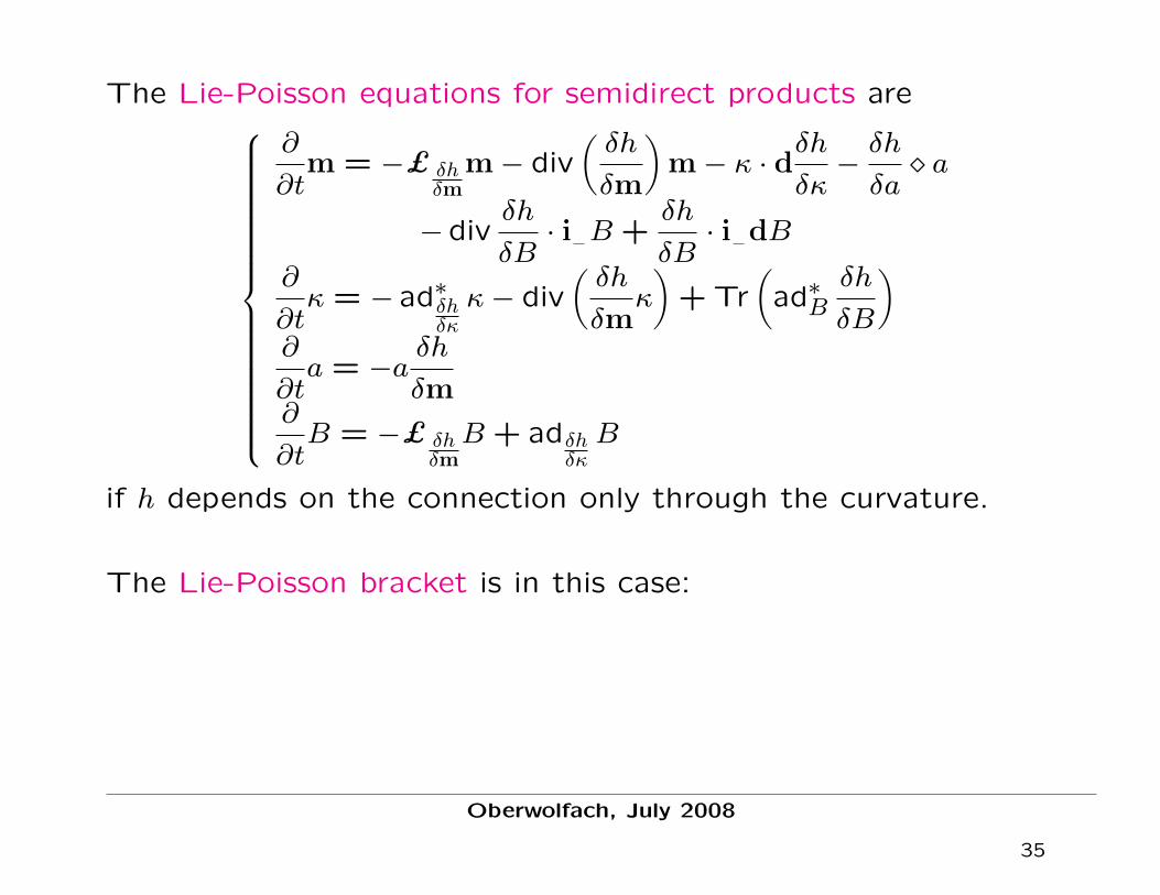
The Lie-Poisson equations for semidirect products are

∂

∂tm = −£ δh

δmm− div

(δh

δm

)m− κ · d

δh

δκ−δh

δa a

−divδh

δB· i B +

δh

δB· i dB

∂


δκ

κ− div(δh

δmκ

)+ Tr

(ad∗B

δh

δB

)∂

∂ta = −a

δh

δm∂

∂tB = −£ δh

δmB + adδh

δκB

if h depends on the connection only through the curvature.

The Lie-Poisson bracket is in this case:


35

f, g(m,κ, a,B) =∫D

m ·[δf

δm,δg

δm

]µ

+∫Dκ ·

(adδf

δκ

δg

δκ+ d

δf

δκ·δg

δm− d

δg

δκ·δf

δm

)µ

+∫Da ·(δf

δa

δg

δm−δg

δa

δf

δm

)µ

+∫D

[(£ δf

δmB − adδf

δκB

)·δg

δB−(£ δg

δmB − adδg

δκB

)·δf

δB

]µ.

The map

(m, ν, a, γ) 7→ (m, ν, a,dγγ)

is a Poisson map relative to the affine Lie-Poisson bracket and this

Lie-Poisson bracket.


36

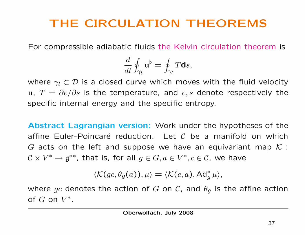
THE CIRCULATION THEOREMS

For compressible adiabatic fluids the Kelvin circulation theorem is

d

dt

∮γt

u[ =∮γtTds,

where γt ⊂ D is a closed curve which moves with the fluid velocity

u, T = ∂e/∂s is the temperature, and e, s denote respectively the

specific internal energy and the specific entropy.

Abstract Lagrangian version: Work under the hypotheses of the

affine Euler-Poincare reduction. Let C be a manifold on which

G acts on the left and suppose we have an equivariant map K :

C × V ∗ → g∗∗, that is, for all g ∈ G, a ∈ V ∗, c ∈ C, we have

〈K(gc, θg(a)), µ〉 = 〈K(c, a),Ad∗g µ〉,

where gc denotes the action of G on C, and θg is the affine action

of G on V ∗.


37

Define the Kelvin-Noether quantity I : C × g× V ∗ → R by

I(c, ξ, a) :=

⟨K(c, a),

δl

δξ(ξ, a)

⟩.

Fixing c0 ∈ C, let ξ(t), a(t) satisfy the affine Euler-Poincare equations

and define g(t) to be the solution of g(t) = TRg(t)ξ(t) and, say,

g(0) = e. Let c(t) = g(t)c0 and I(t) := I(c(t), ξ(t), a(t)). Then

d

dtI(t) =

⟨K(c(t), a(t)),

δl

δa a− dcT

(δl

δa

)⟩.

Abstract Hamiltonian version: Some examples do not admit a

Lagrangian formulation. Nevertheless, a Kelvin-Noether theorem

is still valid for the Hamiltonian formulation. The Kelvin-Noether

quantity is now the mapping J : C × g∗ × V ∗ → R defined by

J(c, µ, a) := 〈K(c, a), µ〉.


38

Fixing c0 ∈ C, let µ(t), a(t) satisfy the affine Lie-Poisson equations

and define g(t) to be the solution of

g(t) = TRg(t)

(δh

δµ

), g(0) = e.

Let c(t) = g(t)c0 and J(t) := J(c(t), µ(t), a(t)). Then

d

dtJ(t) =

⟨K(c(t), a(t)),−

δh

δa a+ dcT

(δh

δa

)⟩.

In the case of dynamics on the group G = Diff(D), the standard

choice for the equivariant map K is

〈K(c, a),m〉 :=∮c

1

ρm,

where c ∈ C = Emb(S1,D), the manifold of all embeddings of the

circle S1 in D, m ∈ Ω1(D), and ρ is advected as (Jη)(ρ η).


39

Consider the affine Euler-Poincare equations for complex fluids.

Suppose that one of the linear advected variables, say ρ, is ad-

vected as (Jη)(ρ η). Then

d

dt

∮ct

1

ρ

δl

δu=∮ct

1

ρ

(−δl

δν· dν +

δl

δa a+

δl

δγ1 γ

),

where ct is a loop in D which moves with the fluid velocity u.

Similarly, consider the affine Lie-Poisson equations for complex flu-

ids. Suppose that one of the linear advected variables, say ρ, is

advected as (Jη)(ρ η). Then

d

dt

∮ct

1

ρm =

∮ct

1

ρ

(−κ · d

δh

δκ−δh

δa a−

δh

δγ1 γ

),

where ct is a loop in D which moves with the fluid velocity u, defined

be the equality

u :=δh

δm.


40

There is also a circulation theorem associated to the variable γ

because of the equation

∂

∂tγ + £uγ = −dν + adν γ.

Let ηt be the flow of the vector field u, let c0 be a loop in D and

let ct := ηt c0. Then, by change of variables, we have

d

dt

∮ctγ =

d

dt

∮c0η∗t γ =

∮c0η∗t (γ + £uγ)

=∮c0η∗t (−dν + adν γ) =

∮ct

adν γ ∈ o,

that is, the γ-circulation law is

d

dt

∮ctγ =

∮ct

adν γ ∈ o.


41

EXAMPLE 1:ERICKSEN-LESLIE EQUATIONS

Liquid crystal state: a distinct phase of matter observed between

the crystalline (solid) and isotropic (liquid) states. Three main

types of liquid crystal states, depending upon the amount of order:

Nematic liquid crystal phase: characterized by rod-like molecules,

no positional order, but tend to point in the same direction.

Cholesteric (or chiral nematic) liquid crystal phase: molecules re-

semble helical springs, which may have opposite chiralities. Molecules

exhibit a privileged direction, which is the axis of the helices.

Smectic liquid crystals are essentially different form both nematics

and cholesterics: they have one more degree of orientational or-

der. Smectics generally form layers within which there is a loss of

positional order, while orientational order is still preserved.Oberwolfach, July 2008

42

Three main theories:

Director theory due to Oseen, Frank, Zocher, Ericksen and Leslie

Micropolar and microstretch theories, due to Eringen, which takeinto account the microinertia of the particles and which is applica-ble, for example, to liquid crystal polymers

Ordered micropolar approach, due to Lhuillier and Rey, which com-bines the director theory with of the micropolar models.

In all that follows D ⊂ R3 and all boundary conditions are ignored:in all integration by parts the boundary terms vanish. We fix avolume form µ on D.

EXAMPLE: DIRECTOR THEORY (nematics, cholesterics)

Assumption: only the direction and not the sense of the moleculesmatter. The preferred orientation of the molecules around a pointis described by a unit vector n : D → S2, called the director, and nand −n are assumed to be equivalent.


43

Ericksen-Leslie equations in a domain D, constraint ‖n‖ = 1, are:

ρ

(∂

∂tu +∇uu

)= grad

∂F

∂ρ−1− ∂j

(ρ∂F

∂n,j·∇n

),

ρJD2

dt2n− 2qn + h = 0,

∂

∂tρ+ div(ρu) = 0

u Eulerian velocity , ρ mass density , n : D → R3 director (n equiva-lent to -n), J microinertia constant, and F (n,n,i) is the free energy .The axiom of objectivity requires that

F (ρ−1, A−1n, A−1∇nA) = F (ρ−1,n,∇n),

for all A ∈ O(3) for nematics, or for all A ∈ SO(3) for cholesterics.

h := ρ∂F

∂n− ∂i

(ρ∂F

∂n,i

).

is the h molecular field. q is unknown and determined by

2q := n · h− ρJ∥∥∥∥Dn

dt

∥∥∥∥2

44

This is seen in the following way.

Take the dot product with n of the second equation to get

2q = ρJn ·D2

dt2n + n · h = n · h− ρJ

∥∥∥∥Dn

dt

∥∥∥∥2

since ‖n‖2 = 1 implies n · Dndt = 0 and hence, taking one more

material derivative gives

n ·D2

dt2n = −

∥∥∥∥Dn

dt

∥∥∥∥2.

Think of the function q in the Ericksen-Leslie equation the way

one regards the pressure in ideal incompressible homogeneous fluid

dynamics, namely, the q is an unknown function determined by the

imposed constraint ‖n‖ = 1.

WHAT IS THE STRUCTURE OF THESE EQUATIONS?


45

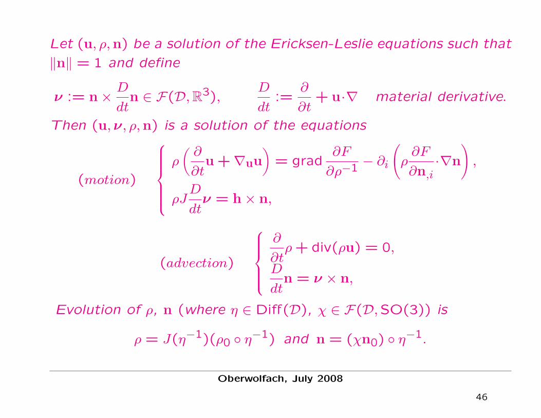
Let (u, ρ,n) be a solution of the Ericksen-Leslie equations such that

‖n‖ = 1 and define

ν := n×D

dtn ∈ F(D,R3),

D

dt:=

∂

∂t+ u·∇ material derivative.

Then (u,ν, ρ,n) is a solution of the equations

(motion)

ρ

(∂

∂tu +∇uu

)= grad

∂F

∂ρ−1− ∂i

(ρ∂F

∂n,i·∇n

),

ρJD

dtν = h× n,

(advection)

∂

∂tρ+ div(ρu) = 0,

D

dtn = ν × n,

Evolution of ρ, n (where η ∈ Diff(D), χ ∈ F(D,SO(3)) is

ρ = J(η−1)(ρ0 η−1) and n = (χn0) η−1.


46

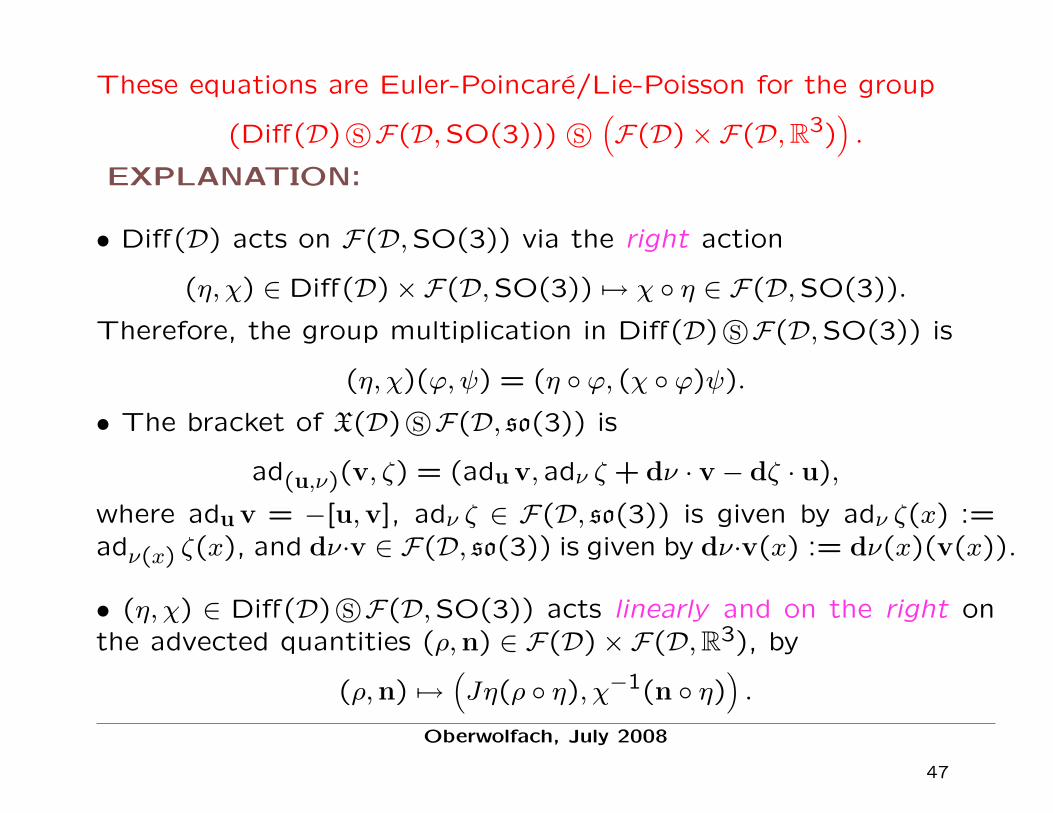
These equations are Euler-Poincare/Lie-Poisson for the group

(Diff(D)sF(D,SO(3))) s(F(D)×F(D,R3)

).

EXPLANATION:

• Diff(D) acts on F(D,SO(3)) via the right action

(η, χ) ∈ Diff(D)×F(D,SO(3)) 7→ χ η ∈ F(D,SO(3)).

Therefore, the group multiplication in Diff(D)sF(D,SO(3)) is

(η, χ)(ϕ,ψ) = (η ϕ, (χ ϕ)ψ).

• The bracket of X(D)sF(D, so(3)) is


where adu v = −[u,v], adν ζ ∈ F(D, so(3)) is given by adν ζ(x) :=adν(x) ζ(x), and dν·v ∈ F(D, so(3)) is given by dν·v(x) := dν(x)(v(x)).

• (η, χ) ∈ Diff(D)sF(D,SO(3)) acts linearly and on the right onthe advected quantities (ρ,n) ∈ F(D)×F(D,R3), by

(ρ,n) 7→(Jη(ρ η), χ−1(n η)

).


47

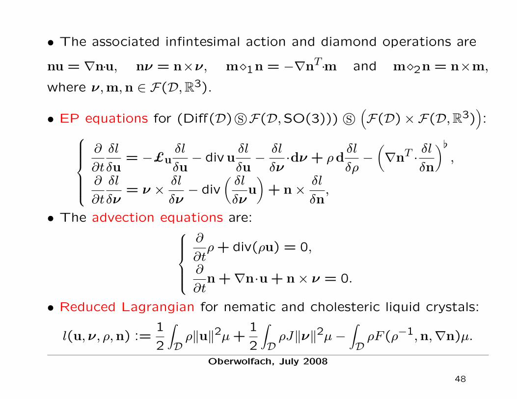
• The associated infintesimal action and diamond operations are

nu = ∇n·u, nν = n×ν, m1n = −∇nT·m and m2n = n×m,

where ν,m,n ∈ F(D,R3).

• EP equations for (Diff(D)sF(D,SO(3))) s(F(D)×F(D,R3)

):

∂

∂t

δl

δu= −£u

δl

δu− div u

δl

δu−δl

δν·dν + ρd

δl

δρ−(∇nT ·

δl

δn

)[,

∂

∂t

δl

δν= ν ×

δl

δν− div

(δl

δνu)

+ n×δl

δn,

• The advection equations are:∂


∂

∂tn +∇n·u + n× ν = 0.

• Reduced Lagrangian for nematic and cholesteric liquid crystals:

l(u,ν, ρ,n) :=1

2

∫Dρ‖u‖2µ+

1

2

∫DρJ‖ν‖2µ−

∫DρF (ρ−1,n,∇n)µ.


48

• The functional derivatives of the Lagrangian l are:

m :=δl

δu= ρu[, κ :=

δl

δν= ρJν,

δl

δρ=

1

2‖u‖2 +

1

2J‖ν‖2−F +

1

ρ

∂F

∂ρ−1,

δl

δn= −ρ

∂F

∂n+∂i

(ρ∂F

∂n,i

)= −h.

• By the Legendre transformation, the Hamiltonian is:

h(m,κ, ρ,n) :=1

2

∫D

1

ρ‖m‖2µ+

1

2J

∫D

1

ρ‖κ‖2µ+

∫DρF (ρ−1,n,∇n)µ.

• The Poisson bracket for liquid crystals is given by:

f,g(m, ρ,κ,n) =∫D

m ·[δf

δm,δg

δm

]µ

+∫D

κ ·(δf

δκ×δg

δκ+ d

δf

δκ·δg

δm− d

δg

δκ·δf

δm

)µ

+∫Dρ

(dδf

δρ·δg

δm− d

δg

δρ·δf

δm

)µ

+∫D

[(n×

δf

δκ+∇n ·

δf

δm

)δg

δn−(n×

δg

δκ+∇n ·

δg

δm

)δf

δn

]µ.


49

• The Kelvin circulation theorem for liquid crystals reads:

d

dt

∮ct

u[ =∮ct

1

ρ∇nT ·h where h = ρ

∂F

∂n− ∂i

(ρ∂F

∂n,i

).

Now do the converse: show that the EP equations imply the Ericksen-Leslie equations. For this one needs to show first that if ν and nare solutions of the EP equations then:

(i) ‖n0‖ = 1 implies ‖n‖ = 1 for all time.

(ii) Ddt(n·ν) = 0. Therefore, n0·ν0 = 0 implies n·ν = 0 for all time.

(iii) Suppose that n0·ν0 = 0 and ‖n0‖ = 1. Then

D

dtn = ν × n becomes ν = n×

D

dtn

and

ρJD

dtν = h× n becomes ρJ

D2

dt2n− 2qn + h = 0.


50

If (u,ν, ρ,n) is a solution of the Euler-Poincare equations with initial

conditions n0 and ν0 satisfying ‖n0‖ = 1 and n0 · ν0 = 0, then

(u, ρ,n) is a solution of the Ericksen-Leslie equations.

The q does not appear in the Euler-Poincare formulation relative to

the variables (u,ν, ρ,n), since in this case, the constraint ‖n‖ = 1

is automatically satisfied.

Consequence of this theorem: the Ericksen-Leslie equations are

obtained by Lagrangian reduction. Right-invariant Lagrangian

L(ρ0,n0) : T [Diff(D)sF(D,SO(3))]→ R

induced by the Lagrangian l (make it right invariant after freezing

the parameters (ρ0,n0)). Assume that ‖n0‖ = 1 and ν0 ·n0 = 0.

A curve (η, χ) ∈ Diff(D)sF(D,SO(3)) is a solution of the Euler-

Lagrange equations for L(ρ0,n0), with initial condition u0, ν0 iff

(u, ν) := (η η−1, χχ−1 η−1)


51

is a solution of the Ericksen-Leslie equations, where

ρ = J(η−1)(ρ0 η−1) and n = (χn0) η−1.

The curve η ∈ Diff(D) describes the Lagrangian motion of the

fluid or macromotion and the curve χ ∈ F(D,SO(3)) describes the

local molecular orientation relative to a fixed reference frame or

micromotion. Standard choice for the initial value of the director is

n0(x) := (0,0,1), for all x ∈ D.

In this case we obtain

n =

χ13χ23χ33

η−1.

This relation is usually taken as a definition of the director, when

the 3-axis is chosen as the reference axis of symmetry.


52

Standard choice for F is the Oseen-Zocher-Frank free energy :

ρF (ρ−1,n,∇n) = K2 (n · curl n)︸︷︷︸chirality

+1

2K11 (div n)2︸︷︷︸

splay

+1

2K22 (n · curl n)2︸︷︷︸

twist

+1

2K33 ‖n× curl n‖2︸︷︷︸

bend

,

where K2 6= 0 for cholesterics and K2 = 0 for nematics. The

free energy can also contain additional terms due to external elec-

tromagnetic fields. The constants K11,K22,K33 are respectively

associated to the three principal distinct director axis deformations

in nematic liquid crystals, namely, splay, twist, and bend.

One-constant approximation : K11 = K22 = K33 = K. Free energy

is, up to the addition of a divergence,

ρF (ρ−1,n,∇n) =1

2K‖∇n‖2.


53

Recall that the molecular field was given by

δl

δn= −ρ

∂F

∂n+ ∂i

(ρ∂F

∂n,i

)= −h.

In the case of the Oseen-Zocher-Frank free energy for nematics

(that is, K2 = 0), the vector h is given by

h =K11 grad div n−K22(A curl n + curl(An))

+K33(B× curl n + curl(n×B)),

where A := n·curl n and B := n× curl n.

In the case of the one-constant approximation, h = −K∆n.


54

EXAMPLE 2:ERINGEN EQUATIONS

This is the micropolar theory of liquid crystals. There is a more

general approach to microfluids, in general.

Microfluids are fluids whose material points are small deformable

particles. Examples of microfluids include liquid crystals, blood,

polymer melts, bubbly fluids, suspensions with deformable particles,

biological fluids.

SKETCH OF ERINGEN’S THEORY

A material particle P in the fluid is characterized by its position X

and by a vector Ξ attached to P that denotes the orientation and

intrinsic deformation of P . Both X and Ξ have their own motions,

X 7→ x = η(X, t) and Ξ 7→ ξ = χ(X,Ξ, t), called respectively the

macromotion and micromotion.Oberwolfach, July 2008

55

The material particles are thought of as very small, so a linear

approximation in Ξ is permissible for the micromotion:

ξ = χ(X, t)Ξ,

where χ(X, t) ∈ GL(3)+ := A ∈ GL(3) | det(A) > 0.

The classical Eringen theory considers only three possible groups in

the description of the micromotion of the particles:

GL(3)+ ⊃ K(3) ⊃ SO(3),

where

K(3) =A ∈ GL(3)+ | there exists λ ∈ R such that AAT = λI3

.

These cases correspond to micromorphic, microstretch, and mi-

cropolar fluids. The Lie group K(3) is a closed subgroup of GL(3)+

that is associated to rotations and stretch.

The general theory admits other groups describing the micromotion.Oberwolfach, July 2008

56

Eringen’s equations for non-dissipative micropolar liquid crystals

ρD

dtul = ∂l

∂Ψ

∂ρ−1− ∂k

(ρ∂Ψ

∂γakγal

), ρσl = ∂k

(ρ∂Ψ

∂γlk

)− εlmnρ

∂Ψ

∂γamγan,

D

dtρ+ ρdiv u = 0,

D

dtjkl + (εkprjlp + εlprjkp)νr = 0,

D

dtγal = ∂lνa + νabγ

bl − γar∂lur.

u ∈ X(D) Eulerian velocity, ρ ∈ F(D) mass density, ν ∈ F(D,R3),

microrotation rate, where we use the standard isomorphism between

so(3) and R3, jkl ∈ F(D,Sym(3)) microinertia tensor (symmetric),

σk, spin inertia is defined by

σk := jklD

dtνl + εklmjmnνlνn =

D

dt(jklνl),

and γ = (γabi ) ∈ Ω1(D, so(3)) wryness tensor. This variable is de-

noted by γ = (γai ) when it is seen as a form with values in R3.

Ψ = Ψ(ρ−1, j, γ) : R× Sym(3)× gl(3)→ R is the free energy.Oberwolfach, July 2008

57

The axiom of objectivity requires that

Ψ(ρ−1, A−1jA,A−1γA) = Ψ(ρ−1, j,γ),

for all A ∈ O(3) (for nematics and nonchiral smectics), or for all

A ∈ SO(3) (for cholesterics and chiral smectics).

These equations are Euler-Poincare/Lie-Poisson for the group

(Diff(D)sF(D,SO(3))) s (F(D)×F(D,Sym(3))×F(D, so(3))) .

EXPLANATION:

• Diff(D) acts on F(D,SO(3)) via the right action

(η, χ) ∈ Diff(D)×F(D,SO(3)) 7→ χ η ∈ F(D,SO(3)).

Therefore, the group multiplication in Diff(D)sF(D,SO(3)) is

(η, χ)(ϕ,ψ) = (η ϕ, (χ ϕ)ψ).


58

• The bracket of X(D)sF(D, so(3)) is


where adu v = −[u,v], adν ζ ∈ F(D, so(3)) is given by adν ζ(x) :=

adν(x) ζ(x), and dν·v ∈ F(D, so(3)) is given by dν·v(x) := dν(x)(v(x)).

• (η, χ) ∈ Diff(D)sF(D,SO(3)) acts linearly and on the right on

the advected quantities (ρ, j) ∈ F(D)×F(D,Sym(3)), by

(ρ, j) 7→(Jη(ρ η), χT (j η)χ

).

• (η, χ) ∈ Diff(D)sF(D,SO(3)) acts on γ ∈ Ω1(D, so(3)) by

γ 7→ χ−1(η∗γ)χ+ χ−1Tχ.

This is a right affine action. Note that γ transforms as a connection.


59

• The reduced Lagrangian

l :[X(D)sF(D,R3)

]s[F(D)⊕F(D,Sym(3))⊕Ω1(D, so(3))

]→ R

is given by

l(u,ν, ρ, j, γ) =1

2

∫Dρ‖u‖2µ+

1

2

∫Dρ (jν ·ν)µ−

∫DρΨ(ρ−1, j, γ)µ.

The affine Euler-Poincare equations for l are:

ρ

(∂

∂tu +∇uu

)= grad

∂Ψ

∂ρ−1− ∂k

(ρ∂Ψ

∂γakγa),

jD

dtν − (jν)× ν = −

1

ρdiv

(ρ∂Ψ

∂γ

)+ γa ×

∂Ψ

∂γa,

∂


D

dtj + [j, ν] = 0,

∂

∂tγ + £uγ + dγν = 0,

which are the Eringen equations after the change of variables γ 7→−γ. Here dγν(v) := dν(v) + [γ(v),ν].


60

L(ρ0,j0,γ0) : T [Diff(D)sF(D,SO(3))]→ R induced by the Lagrangian

l by right translation and freezing the parameters . A curve (η, χ) ∈Diff(D)sF(D,SO(3)) is a solution of the Euler-Lagrange equa-

tions associated to L(ρ0,j0,γ0) if and only if the curve

(u,ν) := (η η−1, χχ−1 η−1) ∈ X(D)sF(D,SO(3))

is a solution of the previous equations with initial conditions (ρ0, j0, γ0).

The evolution of the mass density ρ, the microinertia j, and the

wryness tensor γ is given by

ρ = J(η−1)(ρ0η−1), j =(χj0χ

−1)η−1, γ = η∗

(χγ0χ

−1 + χTχ−1).

If the initial value γ0 is zero, then the evolution of γ is given by

γ = η∗(χTχ−1

).

This relation is usually taken as a definition of γ when using the

Eringen equations without the last one. This is often the case in

the literature.


61

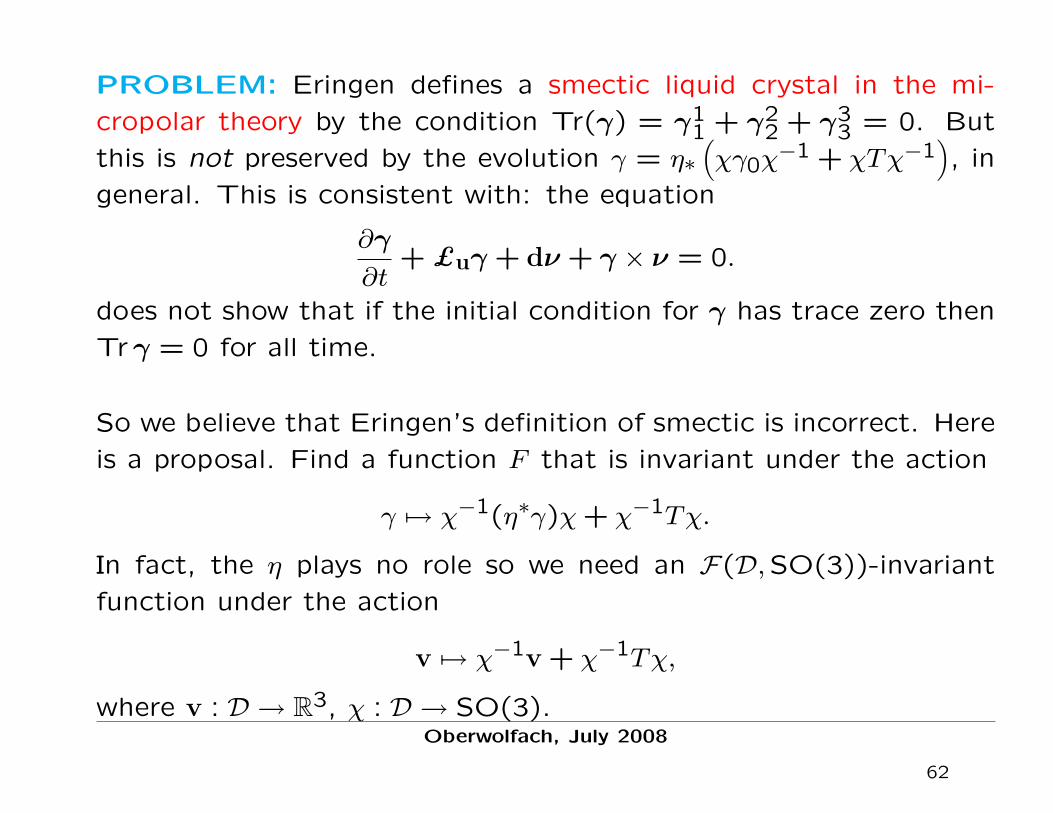
PROBLEM: Eringen defines a smectic liquid crystal in the mi-

cropolar theory by the condition Tr(γ) = γ11 + γ2

2 + γ33 = 0. But

this is not preserved by the evolution γ = η∗(χγ0χ

−1 + χTχ−1), in

general. This is consistent with: the equation

∂γ

∂t+ £uγ + dν + γ × ν = 0.

does not show that if the initial condition for γ has trace zero then

Tr γ = 0 for all time.

So we believe that Eringen’s definition of smectic is incorrect. Here

is a proposal. Find a function F that is invariant under the action

γ 7→ χ−1(η∗γ)χ+ χ−1Tχ.

In fact, the η plays no role so we need an F(D,SO(3))-invariant

function under the action

v 7→ χ−1v + χ−1Tχ,

where v : D → R3, χ : D → SO(3).Oberwolfach, July 2008

62

The affine Lie-Poisson bracket is in this case equal to:

f, g(m,κ, ρ, j) =∫D

m ·[δf

δm,δg

δm

]µ

+∫Dκ ·

(adδf

δκ

δg

δκ+ d

δf

δκ·δg

δm− d

δg

δκ·δf

δm

)µ

+∫Dρ

(d

(δf

δρ

)δg

δm− d

(δg

δρ

)δf

δm

)µ

+∫Dj ·(

div

(δf

δj

δg

δm

)+

[δf

δj,δg

δκ

]− div

(δg

δj

δf

δm

)−[δg

δj,δf

δκ

])µ

+∫D

[(dγδf

δκ+ £ δf

δmγ

)·δg

δγ−(dγδg

δκ+ £ δg

δmγ

)·δf

δγ

]µ

where the brackets in the second to last term denote the usual

commutator bracket of matrices. Circulation theorems are:

d

dt

∮ct

u[ =∮ct

∂Ψ

∂i·di+

∂Ψ

∂γ·i dγ −

1

ρdiv

(ρ∂Ψ

∂γ

)·γ.

andd

dt

∮ct

γ =∮ct

ν × γ

63

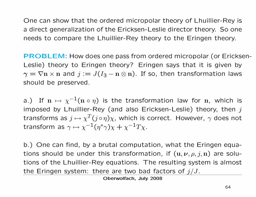
One can show that the ordered micropolar theory of Lhuillier-Rey is

a direct generalization of the Ericksen-Leslie director theory. So one

needs to compare the Lhuillier-Rey theory to the Eringen theory.

PROBLEM: How does one pass from ordered micropolar (or Ericksen-

Leslie) theory to Eringen theory? Eringen says that it is given by

γ = ∇n× n and j := J(I3 − n⊗ n). If so, then transformation laws

should be preserved.

a.) If n 7→ χ−1(n η) is the transformation law for n, which is

imposed by Lhuillier-Rey (and also Ericksen-Leslie) theory, then j

transforms as j 7→ χT (j η)χ, which is correct. However, γ does not

transform as γ 7→ χ−1(η∗γ)χ+ χ−1Tχ.

b.) One can find, by a brutal computation, what the Eringen equa-

tions should be under this transformation, if (u,ν, ρ, j,n) are solu-

tions of the Lhuillier-Rey equations. The resulting system is almost

the Eringen system: there are two bad factors of j/J.Oberwolfach, July 2008

64

lagrangian and hamiltonian structure of complex …marsden/wiki/uploads/oberwolfach/... ·...

Documents