Lale: Consistent Automated Machine LearningGuillaume Baudart, Martin Hirzel, Kiran Kate, Parikshit Ram, and Avraham Shinnar

IBM Research, USA

12345678

910111213

141516

1718

1920

Figure 1: Lale example for consistent automated machine learning, explained in Section 3.

ABSTRACT

Automated machine learning makes it easier for data scientists todevelop pipelines by searching over possible choices for hyperpa-rameters, algorithms, and even pipeline topologies. Unfortunately,the syntax for automated machine learning tools is inconsistentwith manual machine learning, with each other, and with errorchecks. Furthermore, few tools support advanced features such astopology search or higher-order operators. This paper introducesLale, a library of high-level Python interfaces that simplifies andunifies automated machine learning in a consistent way.

1 INTRODUCTION

Machine learning (ML) is widely used in various data science prob-lems. There are many ML operators for data preprocessing (scaling,missing imputation, categorical encoding), feature extraction (prin-cipal component analysis, non-negative matrix factorization), andmodeling (boosted trees, neural networks). A machine learningpipeline consists of one or more operators that take the input datathrough a series of transformations to finally generate predictions.Given the plethora of ML operators (for example, in the widelyused scikit-learn library [5]), the task of finding a good ML pipelinefor the data at hand (which involves not only selecting operatorsbut also appropriately configuring their hyperparameters) can betedious and time consuming if done manually. This has led to awider adoption of automated machine learning (AutoML), with

AutoML Workshop @ KDD’20, August 22–27, 2020, Page 1https://sites.google.com/view/automl2020-workshop/.

the development of novel algorithms (such as SMAC [12], hyper-opt [3], and subsequent recent work [16]), open source libraries(auto-sklearn [10], hyperopt-sklearn [4, 15], TPOT [17]), and evencommercial tools.

Scikit-learn provides a consistent programming model for man-ual ML [5], and various other tools (such as XGBoost [6], Light-GBM [14], and Tensorflow’s tf.keras.wrappers.scikit_learn) maintainconsistency with this model whenever appropriate. AutoML toolsusually feature two pieces – (i) a way to define the search spacecorresponding to the pipeline topology, the operator choices inthat topology, and their respective possible hyperparameter con-figurations, and (ii) an algorithm that explores this search spaceto optimize for predictive performance. Many of these also try tomaintain consistency with the scikit-learn model but only when theuser gives up all control and lets the tool completely automate theML pipeline configuration, eschewing item (i) above. Users oftenwant to retain some control over the automation, for example, tocomply with domain-specific requirements by specifying opera-tors or hyperparameter ranges to search over. While fine-grainedcontrol over the automation is possible (we will discuss examples),users need to manually configure the search space. This searchspace specification differs for each of the different AutoML toolsand differs from the manual programming model.

We believe that proper abstractions are necessary to provide aconsistent programming model across the entire spectrum of con-trolled automation. To this end, we introduce Lale, an open-sourcePython library1, built upon mathematically grounded abstractions

arX

iv:2

007.

0197

7v1

[cs

.LG

] 4

Jul

202

0

AutoML Workshop @ KDD’20, August 22–27, 2020, Page 2 Guillaume Baudart, Martin Hirzel, Kiran Kate, Parikshit Ram, and Avraham Shinnar

1 pipe = Pipeline([2 ('transform', PCA(n_components=4)),3 ('classify', LinearSVC(dual=False, C=10))])4 pipe.fit(train_X, train_y)

Figure 2: Example for manual scikit-learn pipeline.

1 pipe = Pipeline([2 ('transform', PCA()),3 ('classify', RandomForestClassifier())])4 N = [2, 4, 8]5 C = [1, 10, 100, 1000]6 param_grid = [7 {'transform__n_components': N,8 'classify': [LinearSVC(dual=False)],9 'classify__C': C},10 {'transform__n_components': N,11 'classify': [RandomForestClassifier(n_estimators=12)]}]12 grid = GridSearchCV(pipe, param_grid=param_grid)13 grid.fit(train_X, train_y)

Figure 3: Example for scikit-learn GridSearchCV.

of the elements of the pipeline (for example, topology, operator, hy-perparameter configurations), and designed around scikit-learn [5]and JSON Schema [18]. Lale provides a programming interface forspecifying pipelines and search spaces in a consistent manner whileproviding fine-grained control across the automation spectrum. Theabstractions also allow us to provide a consistent programminginterface for capabilities for which no such interface currently exists:(i) search spaces with higher-order operators (operators, such asensembling, that have other operators as hyperparameters), and(ii) search spaces that include search for the pipeline topology viacontext-free grammars [7]. The contributions of this paper are:1. A pipeline specification syntax that is consistent across the au-

tomation spectrum and grounded in established technologies.2. Automatic search space generation from pipelines and schemas

for a consistent experience across existing AutoML tools.3. Higher-order operators (for ensembles, batching, etc.) with auto-

matic AutoML search space generation for nested pipelines.4. A grammar syntax for pipeline topology search that is a natural

extension of the pipeline syntax.Overall, we hope Lale will make data scientists more productive

at finding pipelines that are consistent with their requirements andyield high predictive performance.

2 PROBLEM STATEMENT

Consistency is a core problem for AutoML and existing librariesfall short on this front. This section uses concrete examples frompopular (Auto-)ML libraries to present four shortcomings in existingsystems. We strive to do so in a factual and constructive way.

P1: Provide a consistent programming model across the automationspectrum. There is a spectrum of AutoML ranging from manualmachine learning (no automation) to hyperparameter tuning, op-erator selection, and pipeline topology search. Unfortunately, as

1https://github.com/ibm/lale

1 N = scope.int(hp.qloguniform('N', 2, 8, 1))2 C = hp.lognormal('C', 1, 1000)3 estim = HyperoptEstimator(4 preprocessing=[pca('transform', n_components=N)],5 classifier=hp.choice('classify', [6 liblinear_svc('classify.svc', dual=False, C=C),7 random_forest('classify.rf', n_estimators=12)]),8 algo=tpe.suggest, max_evals=100, trial_timeout=120)9 estim.fit(train_X, train_y)

Figure 4: Example for hyperopt-sklearn.

1 estim = AutoSklearnClassifier(2 include_preprocessors=['pca'],3 include_estimators=['liblinear_svc', 'random_forest'],4 time_left_for_this_task=1800, per_run_time_limit=120)5 estim.fit(train_X, train_y)

Figure 5: Example for auto-sklearn based on SMAC.

users progress across this spectrum, the state-of-the-art librariesrequire them to learn and use different syntax and concepts.

Figure 2 shows an example from the no-automation end of thespectrum using scikit-learn [5]. The code assembles a two-steppipeline of a PCA transformer and a LinearSVC classifier and manuallysets their hyperparameters, for example, n_components=4.

The example in Figure 3 automates hyperparameter tuning andoperator selection using GridSearchCV from scikit-learn. Lines 1–3resemble Figure 2. Lines 4–11 specify a search space, consisting ofa list of two dictionaries. In the first dictionary, Line 7 specifies thelist of values to search over for the n_components hyperparameter ofthe PCA operator; Line 8 specifies the classify step of the pipelineto be a LinearSVC operator; and Line 9 specifies the list of values tosearch over for the C hyperparameter of the LinearSVC operator. Thesecond dictionary is similar, but specifies the RandomForestClassifier.

The syntax for a pipeline (Figure 2 Lines 1–3) differs from that fora search space (Figure 3 Lines 4–11). The mental model is that op-erators and hyperparameters are pre-specified and then the searchspace selectively overwrites them with different choices. To do so,the code uses strings to name steps and hyperparameters, with adouble underscore ('__') name mangling convention to connectthe two. Relying on strings for names can cause hard-to-detectmistakes [1]. In contrast, using a single syntax for both manual andautomated pipelines would make them more consistent and wouldobviate the need for mangled strings to link between the two.

P2: Provide a consistent programming model across different Au-toML tools. Compared to GridSearchCV, Bayesian optimizers such ashyperopt-sklearn [15] and auto-sklearn [10] speed up search usingsmarter search strategies. Unfortunately, each of these AutoMLtools comes with its own syntax and concepts.

Figure 4 shows an example using the hyperopt-sklearn [15] wrap-per for hyperopt [3]. Line 1 specifies a discrete search space Nwith alogarithmic prior, a range from 2..8, and a quantization to multiplesof 1. Line 2 specifies a continuous search space Cwith a logarithmicprior and a range from 1..1000. Line 4 sets the transform step of thepipeline to pca with hyperparameter n_components=N. Lines 5–7 setthe classify step to a choice between linear_svc and random_forest.

Lale: Consistent Automated Machine Learning AutoML Workshop @ KDD’20, August 22–27, 2020, Page 3

Figure 5 shows the same example using auto-sklearn [10]. Whilepower users can use the ConfigurationSpace used by SMAC [12] toadjust search spaces for individual hyperparameters, we elide thisfor brevity. Line 2 sets the preprocessor to 'pca' and Line 3 sets theclassifier to a choice of 'linear_svc' or 'random_forest'.

The syntaxes for the three AutoML tools in Figures 3, 4, and 5 dif-fer. There are three ways to refer to the same operator: PCA, pca(..),and 'pca'. There are three ways to specify an operator choice: a listof dictionaries, hp.choice, and a list of strings. The mental modelvaries from overwriting to nested configuration to string-basedconfiguration. Users must learn new syntax and concepts for eachtool and must rewrite code to switch tools. Moreover, as we con-sider more sophisticated pipelines (beyond the simple two-step onepresented in the example), the search space specifications get evenmore convoluted and diverse between these existing specificationschemes. A unified syntax would make these tools more consistent,easier to learn, and easier to switch. Furthermore, this syntax shouldunify not just AutoML tools but also be consistent with the manualend of the spectrum (P1). More specifically, given that scikit-learnsets the de-facto standard for manual ML, the syntax should bescikit-learn compatible.

P3: Support topology search and higher-order operators in Au-toML tools. The tools previously discussed search operators andhyperparameters but do not optimize the topology of the pipelineitself. There are some tools that do, including TPOT [17], Recipe [8],and AlphaD3M [9]. Unfortunately, their methods for specifyingthe search space are inconsistent with manual machine learningand established tools. TPOT does not allow the user to specify thesearch space for pipeline topologies (the user can specify the set ofoperators and can fix the pipeline topology, disabling the topologysearch). Recipe and AlphaD3M use context-free grammars to spec-ify the search space for the topology, but in a manner inconsistentwith each other or with other levels of automation.

Some transformers (e.g. RFE in Figure 6 Line 7) and estimators(e.g. AdaBoostClassifier) are higher-order : they take other operatorsas arguments. Using the AutoML tools discussed so far to searchinside their nested operators is not straightforward. The aforemen-tioned TPOT, Recipe, and AlphaD3M do not handle higher-orderoperators in their search for pipeline topology.

A unified syntax for topology search and higher-order operatorsthat is a natural extension of the syntax for manual machine learn-ing, algorithm selection, and hyperparameter tuning would makeAutoML more expressive while keeping it consistent.

P4: Check for invalid configurations early and prune them out ofsearch spaces. Even if the search for each hyperparameter uses avalid range in isolation, their combination can violate side con-straints. Worse, these errors may be detected late, wasting time.

Figure 6 shows a misconfigured pipeline: the hyperparametersfor LR in Line 7 are valid in isolation but invalid in combination.Unfortunately, this is not detected when the pipeline is created onLine 7. Instead, when Line 10 tries to fit the pipeline, it first fits thefirst step of the pipeline (see RFE in Line 6). Only then does it try tofit the LR and detect the mistake. This wastes 10 minutes (Line 15).

In contrast, a declarative specification of the side constraintswould both speed up this manual example and enable AutoMLsearch space generators to prune cases that violate constraints,

1234567

89

10111213

1415

16

Figure 6: Example of scikit-learn error checking.

thus speeding up the automated case too. Furthermore, in somesituations, invalid configurations cause more harm than just wastedtime, leading optimizers astray (Section 6). It is possible (with vary-ing levels of difficulty) to incorporate these side constraints withthe search space specification schemes used by the tools discussedearlier, but they each have inconsistent methods for doing this.Moreover, the complexity of these specifications make them errorprone. Additionally, while these side constraints help the optimizer,they do not directly help detect misconfigurations (as in Figure 6).Custom validators would need to be written for each tool.

3 PROGRAMMING ABSTRACTIONS

This section shows Lale’s abstractions for consistent AutoML, ad-dressing the problem statements P1 ∧ P2 ∧ P3 ∧ P4 from Section 2.

3.1 Abstractions for Declarative AutoML

An individual operator is a data science algorithm (aka. a primitiveor a model), which may be a transformer or an estimator such asclassifier or a regressor. Individual operators are modular buildingblocks from libraries such as scikit-learn. Figure 1 Lines 2–6 con-tain several examples, e.g., import LinearSVC as SVM. Mathematically,Lale views an individual operator as a function of the form

indivOp : θhyperparams → Dfit → Din → Dout

This view uses currying: it views an operator as a sequence offunctions each with a single argument and returning the next inthe sequence. An individual operator (e.g., SVM) is a function fromhyperparameters θhyperparams (e.g., dual=False) to a function fromtraining data Dfit (e.g., train_X, train_y) to a function from inputdataDin (e.g., test_X) to output dataDout (e.g., predicted in Figure 1Line 17). In the beginning, all arguments are latent, and each stepin the sequence captures the next argument as given. The scikit-learn terminology for the three curried sub-functions is init, fit, andpredict. Viewing operators as mathematical functions avoids com-plications arising from in-place mutation. It lets us conceptualizebindings as lifecycle: each bound, or captured, argument unlocksthe functionality of the next state in the lifecycle.

A pipeline is a directed acyclic graph (DAG) of operators anda pipeline is itself also an operator. Since a pipeline contains op-erators and is an operator, it is highly composable. Furthermore,

AutoML Workshop @ KDD’20, August 22–27, 2020, Page 4 Guillaume Baudart, Martin Hirzel, Kiran Kate, Parikshit Ram, and Avraham Shinnar

viewing both individual operators and pipelines as special casesof operators makes the concepts more consistent. An exampleis make_pipeline(make_union(PCA, RFC), SVM), which is equivalent to((PCA & RFC) >> ConcatFeatures >> SVM). Here, & is the and combina-tor and >> is the pipe combinator. Combinators make edges moreexplicit and code more concise. An expression x & y composes xand y without introducing additional edges. An expression x >> y

introduces edges from all sinks of subgraph x to all sources of y.Mathematically, Lale views a pipeline as a function of the form

pipeline : θtopology → θhyperparams → Dfit → Din → Dout

This uses currying just like individual operators, plus an additionalθtopology at the start to capture the steps and edges. A pipelineis trainable if both θtopology and θhyperparams are given, i.e., thehyperparameters of all steps have been captured. To fit a trainablepipeline, iterate over the steps in a topological order induced bythe edges. For each step s , let Ds

fit be the training data for the step,which is either the pipeline’s training data if s is a source or thepredecessors’ output data Ds

fit = [Dpout]p∈preds(s) otherwise. Then,

recalling that s is a curried function, calculate strained = s(Dsfit) and

Dsout = strained(Ds

fit). The trained pipeline substitutes trained stepsfor trainable steps in θtopology. To make predictions with a trainedpipeline, simply interpret >> as function composition ◦.

An operator choice is an exclusive disjunction of operators and isitself also an operator. Operator choice specifies algorithm selection,and by being an operator, addresses problem P1 from Section 2. Anexample is (SVM | RFC), where | is the or combinator. Mathematically,Lale views an operator choice as a function of the form

opChoice : θsteps → θhyperparams → Dfit → Din → Dout

This again uses currying. Argument θsteps is the list of operatorsto choose from. The θhyperparams of an operator choice consists ofan indicator for which of its steps is being chosen, along with thehyperparameters for that chosen step. Onceθhyperparams is captured,the operator choice is equivalent to just the chosen step, as shownin the visualization after Figure 1 Line 20.

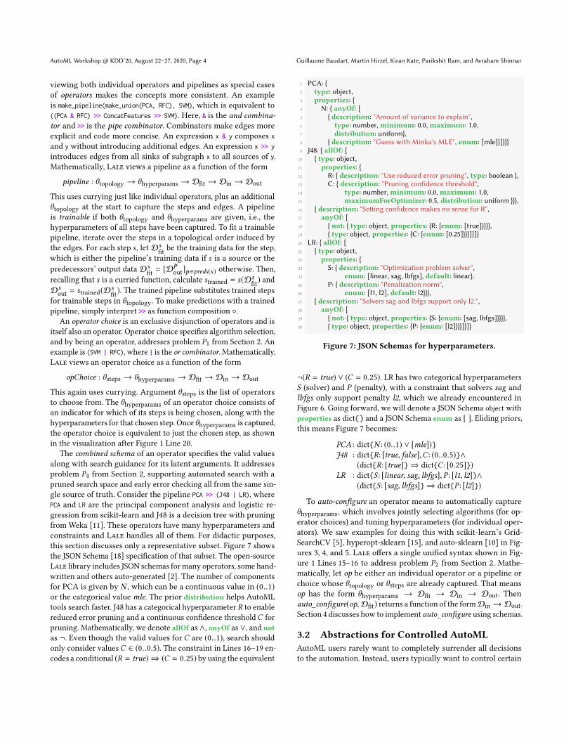
The combined schema of an operator specifies the valid valuesalong with search guidance for its latent arguments. It addressesproblem P4 from Section 2, supporting automated search with apruned search space and early error checking all from the same sin-gle source of truth. Consider the pipeline PCA >> (J48 | LR), wherePCA and LR are the principal component analysis and logistic re-gression from scikit-learn and J48 is a decision tree with pruningfrom Weka [11]. These operators have many hyperparameters andconstraints and Lale handles all of them. For didactic purposes,this section discusses only a representative subset. Figure 7 showsthe JSON Schema [18] specification of that subset. The open-sourceLale library includes JSON schemas for many operators, some hand-written and others auto-generated [2]. The number of componentsfor PCA is given by N , which can be a continuous value in (0..1)or the categorical value mle. The prior distribution helps AutoMLtools search faster. J48 has a categorical hyperparameter R to enablereduced error pruning and a continuous confidence thresholdC forpruning. Mathematically, we denote allOf as ∧, anyOf as ∨, and not

as ¬. Even though the valid values for C are (0..1), search shouldonly consider valuesC ∈ (0..0.5). The constraint in Lines 16–19 en-codes a conditional (R = true) ⇒ (C = 0.25) by using the equivalent

1 PCA: {2 type: object,3 properties: {4 N: { anyOf: [5 { description: "Amount of variance to explain",6 type: number,minimum: 0.0,maximum: 1.0,7 distribution: uniform},8 { description: "Guess with Minka's MLE", enum: [mle]}]}}}9 J48: { allOf: [10 { type: object,11 properties: {12 R: { description: "Use reduced error pruning", type: boolean },13 C: { description: "Pruning confidence threshold",14 type: number,minimum: 0.0, maximum: 1.0,15 maximumForOptimizer: 0.5, distribution: uniform }}},16 { description: "Setting confidence makes no sense for R",17 anyOf: [18 { not: { type: object, properties: {R: {enum: [true]}}}},19 { type: object, properties: {C: {enum: [0.25]}}}]}]}20 LR: { allOf: [21 { type: object,22 properties: {23 S: { description: "Optimization problem solver",24 enum: [linear, sag, lbfgs], default: linear},25 P: { description: "Penalization norm",26 enum: [l1, l2], default: l2}}},27 { description: "Solvers sag and lbfgs support only l2.",28 anyOf: [29 { not: { type: object, properties: {S: {enum: [sag, lbfgs]}}}},30 { type: object, properties: {P: {enum: [l2]}}}]}]}

Figure 7: JSON Schemas for hyperparameters.

¬(R = true) ∨ (C = 0.25). LR has two categorical hyperparametersS (solver) and P (penalty), with a constraint that solvers sag andlbfgs only support penalty l2, which we already encountered inFigure 6. Going forward, we will denote a JSON Schema object withproperties as dict{} and a JSON Schema enum as [ ]. Eliding priors,this means Figure 7 becomes:

PCA : dict{N : (0..1) ∨ [mle])}J48 : dict{R: [true, false],C: (0..0.5)}∧

(dict{R: [true]} ⇒ dict{C: [0.25]})LR : dict{S : [linear, sag, lbfgs], P : [l1, l2]}∧

(dict{S : [sag, lbfgs]} ⇒ dict{P : [l2]})

To auto-configure an operator means to automatically captureθhyperparams, which involves jointly selecting algorithms (for op-erator choices) and tuning hyperparameters (for individual oper-ators). We saw examples for doing this with scikit-learn’s Grid-SearchCV [5], hyperopt-sklearn [15], and auto-sklearn [10] in Fig-ures 3, 4, and 5. Lale offers a single unified syntax shown in Fig-ure 1 Lines 15–16 to address problem P2 from Section 2. Mathe-matically, let op be either an individual operator or a pipeline orchoice whose θtopology or θsteps are already captured. That meansop has the form θhyperparams → Dfit → Din → Dout. Thenauto_configure(op,Dfit) returns a function of the formDin → Dout.Section 4 discusses how to implement auto_configure using schemas.

3.2 Abstractions for Controlled AutoML

AutoML users rarely want to completely surrender all decisionsto the automation. Instead, users typically want to control certain

Lale: Consistent Automated Machine Learning AutoML Workshop @ KDD’20, August 22–27, 2020, Page 5

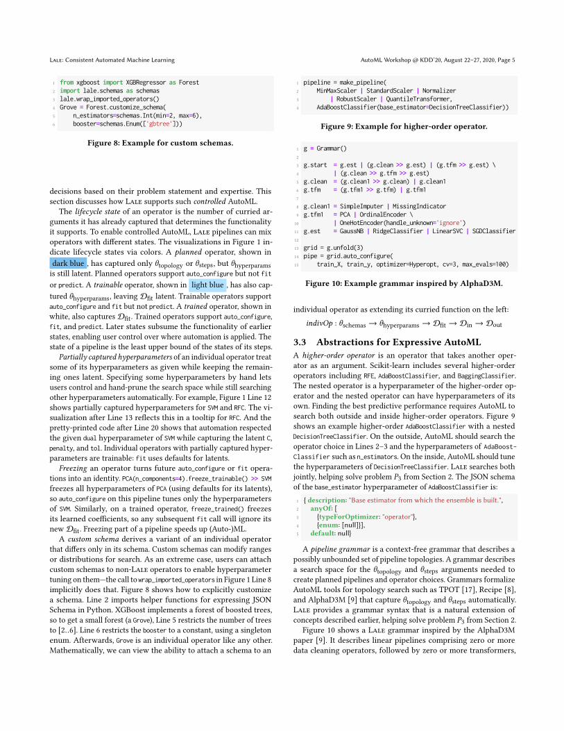
1 from xgboost import XGBRegressor as Forest2 import lale.schemas as schemas3 lale.wrap_imported_operators()4 Grove = Forest.customize_schema(5 n_estimators=schemas.Int(min=2, max=6),6 booster=schemas.Enum(['gbtree']))

Figure 8: Example for custom schemas.

decisions based on their problem statement and expertise. Thissection discusses how Lale supports such controlled AutoML.

The lifecycle state of an operator is the number of curried ar-guments it has already captured that determines the functionalityit supports. To enable controlled AutoML, Lale pipelines can mixoperators with different states. The visualizations in Figure 1 in-dicate lifecycle states via colors. A planned operator, shown indark blue , has captured only θtopology or θsteps, but θhyperparamsis still latent. Planned operators support auto_configure but not fitor predict. A trainable operator, shown in light blue , has also cap-tured θhyperparams, leaving Dfit latent. Trainable operators supportauto_configure and fit but not predict. A trained operator, shown inwhite, also captures Dfit. Trained operators support auto_configure,fit, and predict. Later states subsume the functionality of earlierstates, enabling user control over where automation is applied. Thestate of a pipeline is the least upper bound of the states of its steps.

Partially captured hyperparameters of an individual operator treatsome of its hyperparameters as given while keeping the remain-ing ones latent. Specifying some hyperparameters by hand letsusers control and hand-prune the search space while still searchingother hyperparameters automatically. For example, Figure 1 Line 12shows partially captured hyperparameters for SVM and RFC. The vi-sualization after Line 13 reflects this in a tooltip for RFC. And thepretty-printed code after Line 20 shows that automation respectedthe given dual hyperparameter of SVMwhile capturing the latent C,penalty, and tol. Individual operators with partially captured hyper-parameters are trainable: fit uses defaults for latents.

Freezing an operator turns future auto_configure or fit opera-tions into an identity. PCA(n_components=4).freeze_trainable() >> SVM

freezes all hyperparameters of PCA (using defaults for its latents),so auto_configure on this pipeline tunes only the hyperparametersof SVM. Similarly, on a trained operator, freeze_trained() freezesits learned coefficients, so any subsequent fit call will ignore itsnew Dfit. Freezing part of a pipeline speeds up (Auto-)ML.

A custom schema derives a variant of an individual operatorthat differs only in its schema. Custom schemas can modify rangesor distributions for search. As an extreme case, users can attachcustom schemas to non-Lale operators to enable hyperparametertuning on them—the call towrap_imported_operators in Figure 1 Line 8implicitly does that. Figure 8 shows how to explicitly customizea schema. Line 2 imports helper functions for expressing JSONSchema in Python. XGBoost implements a forest of boosted trees,so to get a small forest (a Grove), Line 5 restricts the number of treesto [2..6]. Line 6 restricts the booster to a constant, using a singletonenum. Afterwards, Grove is an individual operator like any other.Mathematically, we can view the ability to attach a schema to an

1 pipeline = make_pipeline(2 MinMaxScaler | StandardScaler | Normalizer3 | RobustScaler | QuantileTransformer,4 AdaBoostClassifier(base_estimator=DecisionTreeClassifier))

Figure 9: Example for higher-order operator.

1 g = Grammar()2

3 g.start = g.est | (g.clean >> g.est) | (g.tfm >> g.est) \4 | (g.clean >> g.tfm >> g.est)5 g.clean = (g.clean1 >> g.clean) | g.clean16 g.tfm = (g.tfm1 >> g.tfm) | g.tfm17

8 g.clean1 = SimpleImputer | MissingIndicator9 g.tfm1 = PCA | OrdinalEncoder \10 | OneHotEncoder(handle_unknown='ignore')11 g.est = GaussNB | RidgeClassifier | LinearSVC | SGDClassifier12

13 grid = g.unfold(3)14 pipe = grid.auto_configure(15 train_X, train_y, optimizer=Hyperopt, cv=3, max_evals=100)

Figure 10: Example grammar inspired by AlphaD3M.

individual operator as extending its curried function on the left:

indivOp : θschemas → θhyperparams → Dfit → Din → Dout

3.3 Abstractions for Expressive AutoML

A higher-order operator is an operator that takes another oper-ator as an argument. Scikit-learn includes several higher-orderoperators including RFE, AdaBoostClassifier, and BaggingClassifier.The nested operator is a hyperparameter of the higher-order op-erator and the nested operator can have hyperparameters of itsown. Finding the best predictive performance requires AutoML tosearch both outside and inside higher-order operators. Figure 9shows an example higher-order AdaBoostClassifier with a nestedDecisionTreeClassifier. On the outside, AutoML should search theoperator choice in Lines 2–3 and the hyperparameters of AdaBoost-Classifier such as n_estimators. On the inside, AutoML should tunethe hyperparameters of DecisionTreeClassifier. Lale searches bothjointly, helping solve problem P3 from Section 2. The JSON schemaof the base_estimator hyperparameter of AdaBoostClassifier is:1 { description: "Base estimator from which the ensemble is built.",2 anyOf: [3 {typeForOptimizer: "operator"},4 {enum: [null]}],5 default: null}

A pipeline grammar is a context-free grammar that describes apossibly unbounded set of pipeline topologies. A grammar describesa search space for the θtopology and θsteps arguments needed tocreate planned pipelines and operator choices. Grammars formalizeAutoML tools for topology search such as TPOT [17], Recipe [8],and AlphaD3M [9] that capture θtopology and θsteps automatically.Lale provides a grammar syntax that is a natural extension ofconcepts described earlier, helping solve problem P3 from Section 2.

Figure 10 shows a Lale grammar inspired by the AlphaD3Mpaper [9]. It describes linear pipelines comprising zero or moredata cleaning operators, followed by zero or more transformers,

AutoML Workshop @ KDD’20, August 22–27, 2020, Page 6 Guillaume Baudart, Martin Hirzel, Kiran Kate, Parikshit Ram, and Avraham Shinnar

1 g = Grammar()2

3 g.start = g.process >> g.features >> g.model4 g.process = g.process1 | ((g.process1 & g.process) >> Concat)5 g.features = g.feature1 \6 | (((g.feature1 | g.est) & g.features) >> Concat)7 g.model = g.est8

9 g.process1 = NoOp | MinMax | Standard | Norm | Robust10 g.feature1 = NoOp | PCA | PolynomialFeatures | Nystroem11 g.est = GaussianNB | GradientBoostingClassifier | KNN \12 | RandomForestClassifier | ExtraTreesClassifier \13 | QDA | PassiveAggressiveClassifier \14 | DecisionTreeClassifier | LR | XGB | LGBM | SVC

Figure 11: Example grammar inspired by TPOT.

followed by exactly one estimator. This is implemented via recursivenon-terminals: g.clean on Line 5 is a recursive definition, and so isg.tfm on Line 6, implementing a search space with sub-pipelines ofunbounded length. While AlphaD3M uses reinforcement learningto search over this grammar, Figure 10 does something far lesssophisticated. Line 13 unfolds the grammar to depth 3, obtaining abounded planned pipeline, and Line 14 searches that using hyperopt,with no further modifications required.

Figure 11 shows a Lale grammar inspired by TPOT [17]. It de-scribes possibly non-linear pipelines, which use not only >> but alsothe & combinator. Recall that (x & y) >> Concat applies both x andy to the same data and then concatenates the features from both.Besides transformers, Line 6 also uses estimators with &, turningtheir predictions into features for downstream operators. This isnot supported in scikit-learn pipelines but is supported in Lale.

Progressive disclosure is a design technique that makes thingseasier to use by only requiring users to learn new features when andas they need them. The starting point for Lale is manual machinelearning, and thus, the scikit-learn code in Figure 2 is also validLale code. User needs to learn zero new features if they do notuse AutoML. To use algorithm selection, users only need to learnabout the | combinator and the auto_configure function. To expresspipelines more concisely, users can learn about the >> and & combi-nators, but those are optional syntactic sugar for make_pipeline andmake_union from scikit-learn. To use hyperparameter tuning, usersonly need to learn about wrap_imported_operators. To exercise morecontrol over the search space, users can learn about freeze andcustom schemas. While schemas are a non-trivial concept, Laleexpresses them in JSON Schema [18], which is a widely-adoptedand well-documented standard proposal. To use higher-order opera-tors, users need not learn new syntax, as Lale supports scikit-learnsyntax for them. Finally, to use grammars, users need to add ‘g.’ infront of their pipeline definitions; however, all the other features,such as the | combinator and the auto_configure function, continueto work the same with or without grammars.

4 SEARCH SPACE GENERATION

This section describes how to map the programming model fromSection 3 to work directly with three popular AutoML tools: scikit-learn’s GridSearchCV [5], hyperopt [4], and SMAC [12], the librarybehind auto-sklearn [10].

4.1 From Grammars to Planned Pipelines

Lale offers two approaches for using a grammar with GridSearch-CV, hyperopt, and SMAC: unfolding and sampling. Both approachesproduce a planned pipeline, which can be directly used as theinput for the compiler in Section 4.2. Unfolding and sampling aremerely intended as proof-of-concept baseline implementations. Inthe future, we will also explore integrating Lale grammars directlywith AutoML tools that support them, such as AlphaD3M [9].

Unfolding first expands the grammar to a given depth, such as 3in the example from Figure 10 Line 13. Then, it prunes all disjunctscontaining unresolved nonterminals, so that only planned Laleoperators (individual, pipeline, or choice) remain.

Sampling traverses the grammar by following each nonterminal,picking a random step in each choice, and unfolding each pipeline.The result is a planned pipeline without any operator choices.

4.2 From Planned Pipelines to Existing Tools

This section sketches how to map a planned pipeline (which in-cludes a topology, steps for operator choices, and schemas for indi-vidual operator) to a search space in the format required by Grid-SearchCV, hyperopt, or SMAC. The running example for this sec-tion is the pipeline PCA >> (J48 | LR) with the individual operatorschemas in Figure 7.

Lale’s search space generator has two phases: normalizer andbackend. The normalizer translates the schemas of individual oper-ators separately. The backend combines the schemas for the entirepipeline and finally generates a tool-specific search space.

The normalizer processes the schema for an individual operatorin a bottom-up pass. The desired end result is a search space inLale’s normal form, which is ∨(dict{cat∗, cont∗}∗). At each level,the normalizer simplifies children and hoists disjunctions up.

PCA:dict{N : (0..1)} ∨ dict{N : [mle]}J48 :dict{R: [false],C: (0..0.5)} ∨ dict{R: [true, false],C: [0.25]}LR :dict{S : [linear], P : [l1, l2]} ∨ dict{S : [linear, sag, lbfgs], P : [l2]}

The backend starts by first combining the search spaces for alloperators in the pipeline. Each pipeline becomes a ‘dict’ over itssteps; each operator choice becomes an ‘∨’ over its steps with addeddiscriminantsD to track what was chosen; and each individual oper-ator simply comes from the normalizer. This yields an intermediaterepresentation (IR) whose nesting structure reflects the operatornesting of the original pipeline. For our running example, this is:

dict

0: dict{N : (0..1)} ∨ dict{N : [mle]}

1:©­­­«(dict{D: [J48],R: [false],C: (0..0.5)} ∨dict{D: [J48],R: [true, false],C: [0.25]}

)∨(

dict{D: [LR], S : [linear], P : [l1, l2]} ∨dict{D: [LR], S : [linear, sag, lbfgs], P : [l2]}

) ª®®®¬

The remainder of the backend is specific to the targeted AutoMLtools, which the following text describes one by one.

The hyperopt backend of Lale is the simplest because hyperoptsupports nested search space specifications that are conceptuallysimilar to the Lale IR. For instance, an exclusive disjunction ‘∨’from the IR can be translated into a hyperopt hp.choice, an examplefor which occurs in Figure 4 Line 5. Similarly, a ‘dict’ from the IR canbe translated into a Python dictionary that hyperopt understands.

Lale: Consistent Automated Machine Learning AutoML Workshop @ KDD’20, August 22–27, 2020, Page 7

For working with higher-order operators, Lale adds additionalmarkers that enable it to reconstruct nested operators later.

The SMAC backend has to flatten Lale’s nested IR into a grid ofdisjuncts with discriminants D. To do this, it internally uses a namemangling encoding that extends the __mangling of scikit-learn, anexample for which occurs in Figure 3 Line 7. Each element of thegrid needs to be a simple ‘dict’ with no further nesting. For ourrunning example, the result in mathematical notation is:

dict{N : (0..1),D: [J48],R: [false], C: (0..0.5)}∨ dict{N : (0..1),D: [J48],R: [true, false], C: [0.25] }∨ dict{N : [mle], D: [J48],R: [false], C: (0..0.5)}∨ dict{N : [mle], D: [J48],R: [true, false], C: [0.25] }∨ dict{N : (0..1),D: [LR], S : [linear], P : [l1, l2] }∨ dict{N : (0..1),D: [LR], S : [linear, sag, lbfgs], P : [l2] }∨ dict{N : [mle], D: [LR], S : [linear], P : [l1, l2] }∨ dict{N : [mle], D: [LR], S : [linear, sag, lbfgs], P : [l2] }

Next, the SMAC backend adds conditionals that tell the Bayesianoptimizer which variables are relevant for which disjunct, andfinally outputs the search space in SMAC’s PCS format.

The GridSearchCV backend starts from the same flattened gridrepresentation that is also used by the SMAC backend. Then, itdiscretizes each continuous hyperparameter into a categorical byfirst including the default and then sampling a user-configurablenumber of additional values from its range and prior distribution(such as uniform in Figure 7 Line 7). The generated search space inmathematical notation is:

dict{N : [0.50, 0.01],D: [J48],R: [false],C: [0.25, 0.01]}∨ dict{N : [0.50, 0.01],D: [J48],R: [true, false],C: [0.25]}∨ dict{N : [mle],D: [J48],R: [false],C: [0.25, 0.01]}∨ dict{N : [mle],D: [J48],R: [true, false],C: [0.25]}∨ dict{N : [0.50, 0.01],D: [LR], S : [linear], P : [l1, l2]}∨ dict{N : [0.50, 0.01],D: [LR], S : [linear, sag, lbfgs], P : [l2]}∨ dict{N : [mle],D: [LR], S : [linear], P : [l1, l2]}∨ dict{N : [mle],D: [LR], S : [linear, sag, lbfgs], P : [l2]}

5 IMPLEMENTATION

This section highlights some of the trickier parts of the Lale imple-mentation, which is entirely in Python.

To implement lifecycle states, Lale uses Python subclassing. Forexample, the Trainable is a subclass of Planned, adding a fitmethod.Subclassing lets users treat an operator as also still belonging to anearlier state, e.g., in a mixed-state pipeline. The Lale implementa-tion adds Python 3 type hints so users can get additional help fromtools such as MyPy, PyCharm, or VSCode.

To implement the combinators >>, &, and |, Lale uses Python’soverloaded __rshift__, __and__, and __or__ methods. Python onlysupports overriding these as instance methods. Therefore, unlike inscikit-learn, Lale planned operators are object instances, not classes.This required emulating the scikit-learn __init__with __call__.

The implementation carefully avoids in-place mutation of op-erators by methods such as auto_configure, fit, customize_schema, orunfold. This prevents unintended side effects and keeps the imple-mentation consistent with the mathematical function abstractionsfrom Section 3.1. Unfortunately, in scikit-learn, fit does in-placemutation, so for compatibility, Lale supports that but with a depre-cation warning.

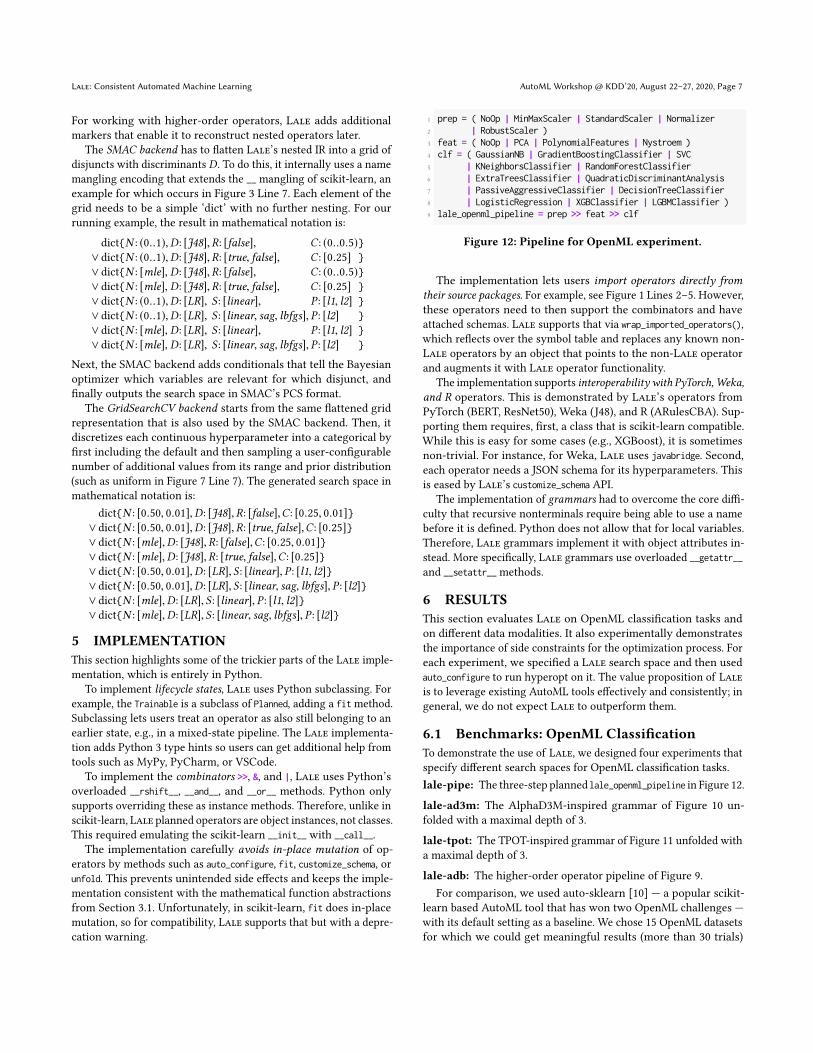
1 prep = ( NoOp | MinMaxScaler | StandardScaler | Normalizer2 | RobustScaler )3 feat = ( NoOp | PCA | PolynomialFeatures | Nystroem )4 clf = ( GaussianNB | GradientBoostingClassifier | SVC5 | KNeighborsClassifier | RandomForestClassifier6 | ExtraTreesClassifier | QuadraticDiscriminantAnalysis7 | PassiveAggressiveClassifier | DecisionTreeClassifier8 | LogisticRegression | XGBClassifier | LGBMClassifier )9 lale_openml_pipeline = prep >> feat >> clf

Figure 12: Pipeline for OpenML experiment.

The implementation lets users import operators directly fromtheir source packages. For example, see Figure 1 Lines 2–5. However,these operators need to then support the combinators and haveattached schemas. Lale supports that via wrap_imported_operators(),which reflects over the symbol table and replaces any known non-Lale operators by an object that points to the non-Lale operatorand augments it with Lale operator functionality.

The implementation supports interoperability with PyTorch,Weka,and R operators. This is demonstrated by Lale’s operators fromPyTorch (BERT, ResNet50), Weka (J48), and R (ARulesCBA). Sup-porting them requires, first, a class that is scikit-learn compatible.While this is easy for some cases (e.g., XGBoost), it is sometimesnon-trivial. For instance, for Weka, Lale uses javabridge. Second,each operator needs a JSON schema for its hyperparameters. Thisis eased by Lale’s customize_schemaAPI.

The implementation of grammars had to overcome the core diffi-culty that recursive nonterminals require being able to use a namebefore it is defined. Python does not allow that for local variables.Therefore, Lale grammars implement it with object attributes in-stead. More specifically, Lale grammars use overloaded __getattr__

and __setattr__methods.

6 RESULTS

This section evaluates Lale on OpenML classification tasks andon different data modalities. It also experimentally demonstratesthe importance of side constraints for the optimization process. Foreach experiment, we specified a Lale search space and then usedauto_configure to run hyperopt on it. The value proposition of Laleis to leverage existing AutoML tools effectively and consistently; ingeneral, we do not expect Lale to outperform them.

6.1 Benchmarks: OpenML Classification

To demonstrate the use of Lale, we designed four experiments thatspecify different search spaces for OpenML classification tasks.lale-pipe: The three-step plannedlale_openml_pipeline in Figure 12.

lale-ad3m: The AlphaD3M-inspired grammar of Figure 10 un-folded with a maximal depth of 3.

lale-tpot: The TPOT-inspired grammar of Figure 11 unfolded witha maximal depth of 3.

lale-adb: The higher-order operator pipeline of Figure 9.For comparison, we used auto-sklearn [10] — a popular scikit-

learn based AutoML tool that has won two OpenML challenges —with its default setting as a baseline. We chose 15 OpenML datasetsfor which we could get meaningful results (more than 30 trials)

AutoML Workshop @ KDD’20, August 22–27, 2020, Page 8 Guillaume Baudart, Martin Hirzel, Kiran Kate, Parikshit Ram, and Avraham Shinnar

Table 1: Accuracy for 15 OpenML classification tasks

Absolute accuracy (mean and standard deviation over 5 runs) 100 ∗ (accuracy/autoskl − 1)Dataset autoskl lale-pipe lale-tpot lale-ad3m lale-adb askl-adb lale-pipe lale-tpot lale-ad3m lale-adb

australian 85.09 (0.44) 85.44 (0.72) 85.88 (0.57) 86.84 (0.00) 86.05 (1.62) 84.74 (3.11) 0.41 0.93 2.06 1.13blood 77.89 (1.39) 76.28 (5.22) 77.49 (2.46) 74.74 (0.74) 77.09 (0.74) 74.74 (0.84) -2.08 -0.52 -4.05 -1.04breast-cancer 73.05 (0.58) 71.16 (1.20) 71.37 (1.15) 69.47 (3.33) 70.95 (2.05) 72.42 (0.47) -2.59 -2.31 -4.90 -2.88car 99.37 (0.10) 98.25 (1.16) 99.12 (0.12) 92.71 (0.63) 98.28 (0.26) 98.25 (0.25) -1.13 -0.25 -6.70 -1.09credit-g 76.61 (1.20) 74.85 (0.52) 74.12 (0.55) 74.79 (0.40) 76.06 (1.27) 76.24 (1.02) -2.29 -3.24 -2.37 -0.71diabetes 77.01 (1.32) 77.48 (1.51) 76.38 (1.11) 77.87 (0.18) 75.98 (0.48) 75.04 (1.03) 0.61 -0.82 1.12 -1.33hill-valley 99.45 (0.97) 99.25 (1.15) 100.0 (0.00) 96.80 (0.21) 100.00 (0.00) 99.10 (0.52) -0.20 0.55 -2.66 0.55jungle-chess 88.06 (0.24) 90.29 (0.00) 88.90 (2.05) 74.14 (2.02) 89.41 (2.29) 86.87 (0.20) 2.54 0.96 -15.80 1.53kc1 83.79 (0.31) 83.48 (0.75) 83.48 (0.54) 83.62 (0.23) 83.30 (0.36) 84.02 (0.31) -0.38 -0.38 -0.21 -0.58kr-vs-kp 99.70 (0.04) 99.34 (0.07) 99.43 (0.00) 96.83 (0.14) 99.51 (0.10) 99.47 (0.16) -0.36 -0.27 -2.87 -0.19mfeat-factors 98.70 (0.08) 97.58 (0.28) 97.18 (0.50) 97.55 (0.07) 97.52 (0.40) 97.94 (0.08) -1.14 -1.54 -1.17 -1.20phoneme 90.31 (0.39) 89.06 (0.67) 89.56 (0.36) 76.57 (0.00) 90.11 (0.45) 91.36 (0.21) -1.39 -0.83 -15.20 -0.22shuttle 87.27 (11.6) 99.94 (0.01) 99.93 (0.04) 99.89 (0.00) 99.98 (0.00) 99.97 (0.01) 14.51 14.50 14.45 14.56spectf 87.93 (0.86) 87.24 (1.12) 88.45 (2.25) 83.62 (6.92) 88.45 (2.63) 89.66 (2.92) -0.78 0.59 -4.90 0.59sylvine 95.42 (0.21) 95.00 (0.61) 94.41 (0.75) 91.31 (0.12) 95.15 (0.20) 95.07 (0.14) -0.45 -1.07 -4.31 -0.29

using the default settings of Auto-sklearn. The selected datasetscomprise 5 simple classification tasks (test accuracy > 90% in allour experiments) and 10 harder tasks (test accuracy < 90%). Foreach experiment, we used a 66% − 33% validation-test split, and a5-fold cross validation on the validation split during optimization.Experiments were run on a 32 cores (2.0GHz) virtual machine with128GB memory, and for each task, the total optimization time wasset to 1 hour with a timeout of 6 minutes per trial.

Table 1 presents the results of our experiments. For each ex-periment, we report the test accuracy of the best pipeline foundaveraged over 5 runs. Note that for the shuttle dataset, 3 out of 5runs of auto-sklearn resulted in a MyDummyClassifier being returnedas the result. Since we were trying to evaluate the default settings,we did not attempt debugging it, but according to the tool’s issuelog, other users have encountered it before. The column askl-adbreports the accuracy of auto-sklearn when the set of classifiers islimited to AdaBoost with only data pre-processing. These resultsare presented for comparison with the lale-adb experiments, asthe data preprocessing operators in Figure 9 were chosen to matchthose of auto-sklearn as much as possible. Also note that the defaultsetting for auto-sklearn uses meta-learning.

The results show that carefully crafted search spaces (e.g., TPOT-inspired grammar, or pipelines with higher-order operators) and off-the-shelf optimizers such as hyperopt can achieve accuracies thatare competitive with state-of-the-art tools. These experiments thusvalidate Lale’s controlled approach to AutoML as an alternative toblack-box solutions. In addition, these experiments illustrate thatLale is modular enough to easily express and compare multiplesearch spaces for a given task.

6.2 Case Studies: Other Modalities

While all the examples so far focused on tasks for tabular datasets,the core contribution of Lale is not limited to those. This sectiondemonstrates Lale’s versatility on three datasets from differentmodalities. Table 2 summarizes the results.Text. We used the Drug Review dataset for predicting a ratinggiven by a patient to a drug. The Drug Review dataset has a text col-umn calledreview, to which the pipeline applies eitherTfidfVectorizer

Table 2: Performance of the best pipeline using Lale with

hyperopt. The mean and stdev are over 3 runs.

modality dataset mean stdev metric

Text Drug Review 1.9237 0.06 test RMSEImage CIFAR-10 93.53% 0.11 test accuracyTime-series Epilepsy 73.15% 8.2 test accuracy

from scikit-learn or a pretrained BERT embeddings, which is a textembedding based on neural networks. The dataset also has numericcolumns, which are concatenated with the result of the embedding.

1 planned_pipeline = (2 Project(columns=['review']) >> (BERT | TfidfVectorizer)3 & Project(columns={'type': 'number'})4 ) >> Cat >> (LinearRegression | XGBRegressor)

Image. We used the CIFAR-10 computer vision dataset. We pickedthe ResNet50 deep-learning model, since it has been shown to dowell on CIFAR-10. Our experiments kept the architecture of ResNet50fixed and tuned learning-procedure hyperparameters.

Time-series. We used the Epilepsy dataset, a subset of the TUHSeizure Corpus, for classifying seizures by onset location (general-ized or focal). We used a three-step pipeline:

1 planned = Window \2 >> (KNeighborsClassifier| XGBClassifier| LogisticRegression) \3 >> Voting

We implemented a popular pre-processing method [19] in a Windowoperator with three hyperparametersW , O , and T . Note that thistransformer leads to multiple samples per seizure. Hence, duringevaluation, each seizure is classified by taking a vote of the predic-tions made by each sample generated from it.

6.3 Effect of Side Constraints on Convergence

Lale’s search space compiler takes rich hyperparameter schemasincluding side constraints and translates them into semanticallyequivalent search spaces for different AutoML tools. This raises thequestion of how important those side constraints are in practice.

Lale: Consistent Automated Machine Learning AutoML Workshop @ KDD’20, August 22–27, 2020, Page 9

Figure 13: Convergence with planned pipeline LR | KNN.

Figure 14: Convergence with planned pipeline J48 | LR | KNN.

To explore this, we did an ablation study where we generated notjust the constrained search spaces that are default with Lale butalso unconstrained search spaces that drop side constraints. Withhyperopt on the unconstrained search space, some iterations areunsuccessful due to exceptions, for which we reported np.float.max

loss. Figure 13 plots the convergence for the Car dataset on theplanned pipeline LR | KNN. Both of these operators have a few sideconstraints. Whereas the unconstrained search space causes someinvalid points early in the search, the two curves more-or-lesscoincide after about two dozen iterations. The story looks verydifferent in Figure 14 when adding a third operator J48 | LR | KNN.In the unconstrained case, J48 has many more invalid runs, causinghyperopt to see so many np.float.max loss values from J48 that itgives up on it. In the constrained case, on the other hand, J48 has noinvalid runs, and hyperopt eventually realizes that it can configureJ48 to obtain substantially better performance.

6.4 Dataset Details

In order to be specific about the exact datasets for reproducibility,Table 3 report the URLs for accessing those.

7 RELATEDWORK

There are various search tools, designed around scikit-learn [5],and each usually focused on a particular novel optimization algo-rithm. Auto-sklearn [10] uses the search space specification andoptimization algorithm of SMAC [12]. Hyperopt-sklearn [15] usesits own search space specification scheme and a novel optimizerbased on Tree-structured Parzen Estimators (TPE) [3]. Scikit-learnalso comes with its own GridSearchCV and RandomizedSearchCVclasses. Auto-Weka [20] is a predecessor of auto-sklearn that alsouses SMAC but operates on operators from Weka [11] instead of

Table 3: Dataset details for reproducibility.

Dataset URL

australian https://www.openml.org/d/40981blood https://www.openml.org/d/1464breast-cancer https://www.openml.org/d/13car https://www.openml.org/d/40975credit-g https://www.openml.org/d/31diabetes https://www.openml.org/d/37hill-valley https://www.openml.org/d/1479jungle-chess https://www.openml.org/d/41027kc1 https://www.openml.org/d/1067kr-vs-kp https://www.openml.org/d/3mfeat-factors https://www.openml.org/d/12phoneme https://www.openml.org/d/1489shuttle https://www.openml.org/d/40685spectf https://www.openml.org/d/337sylvine https://www.openml.org/d/41146

CIFAR-10 https://en.wikipedia.org/wiki/CIFAR-10Drug Review https://archive.ics.uci.edu/ml/datasets/Drug+Revi+

Dataset+%28Drugs.com%29Epilepsy https://www.ncbi.nlm.nih.gov/pmc/articles/

PMC6246677

scikit-learn. TPOT [17] is designed around scikit-learn and usesgenetic programming to search for pipeline topologies and operatorchoices. This usually leads to the generation of many misconfig-ured pipelines, wasting execution time. RECIPE [8] prunes awaythe misconfigurations to save execution time by validating gener-ated pipelines with a grammar for linear pipelines. AlphaD3M [9]makes use of a grammar in a generative manner (instead of justfor validation) with a deep reinforcement learning based algorithm.Katz et al. [13] similarly use a grammar for Lale pipelines with AIplanning tools. In contrast to these tools, the contribution of thispaper is not a novel optimization algorithm but rather a more con-sistent programming model with search space generation targetingexisting tools.

8 CONCLUSION

This paper describes Lale, a library for semi-automated data sci-ence. Lale contributes a syntax that is consistent with scikit-learn,but extends it to support a broad spectrum of automation includingalgorithm selection, hyperparameter tuning, and topology search.Lale works by automatically generating search spaces for estab-lished AutoML tools, extending their capabilities to grammar-basedsearch and to search inside higher-order operators. The experi-ments show that search spaces crafted using Lale achieve resultsthat are competitive with state-of-the-art tools while offering moreversatility.

AutoML Workshop @ KDD’20, August 22–27, 2020, Page 10 Guillaume Baudart, Martin Hirzel, Kiran Kate, Parikshit Ram, and Avraham Shinnar

REFERENCES

[1] Guillaume Baudart, Martin Hirzel, Kiran Kate, Louis Mandel, and Avraham Shin-nar. 2019. Machine Learning in Python with No Strings Attached. In Work-shop on Machine Learning and Programming Languages (MAPL). 1–9. https://doi.org/10.1145/3315508.3329972

[2] Guillaume Baudart, Peter Kirchner, Martin Hirzel, and Kiran Kate. 2020. Min-ing Documentation to Extract Hyperparameter Schemas. In ICML Workshop onAutomated Machine Learning (AutoML@ICML). https://arxiv.org/abs/2006.16984

[3] James Bergstra, Rémi Bardenet, Yoshua Bengio, and Balázs Kégl. 2011. Algo-rithms for Hyper-Parameter Optimization. In Conference on Neural InformationProcessing Systems (NIPS). http://papers.nips.cc/paper/4443-algorithms-for-hyper-parameter-optimizat

[4] James Bergstra, Brent Komer, Chris Eliasmith, Dan Yamins, and David D. Cox.2015. Hyperopt: a Python Library for Model Selection and HyperparameterOptimization. Computational Science & Discovery 8, 1 (2015). http://dx.doi.org/10.1088/1749-4699/8/1/014008

[5] Lars Buitinck, Gilles Louppe, Mathieu Blondel, Fabian Pedregosa, AndreasMueller, Olivier Grisel, Vlad Niculae, Peter Prettenhofer, Alexandre Gramfort,Jaques Grobler, Robert Layton, Jake VanderPlas, Arnaud Joly, Brian Holt, andGaël Varoquaux. 2013. API Design for Machine Learning Software: Experiencesfrom the scikit-learn Project. https://arxiv.org/abs/1309.0238

[6] Tianqi Chen and Carlos Guestrin. 2016. XGBoost: A Scalable Tree BoostingSystem. In Conference on Knowledge Discovery and Data Mining (KDD). 785–794.http://doi.acm.org/10.1145/2939672.2939785

[7] Noam Chomsky. 1956. Three models for the description of language. IRE Trans-actions on Information Theory 2, 3 (1956), 113–124.

[8] Alex G. C. de Sá, Walter José G. S. Pinto, Luiz Otavio V. B. Oliveira, and Gisele L.Pappa. 2017. RECIPE: A Grammar-Based Framework for Automatically EvolvingClassification Pipelines. In European Conference on Genetic Programming (EuroGP).246–261. https://link.springer.com/chapter/10.1007/978-3-319-55696-3_16

[9] Iddo Drori, Yamuna Krishnamurthy, Raoni Lourenco, Remi Rampin, KyunghyunCho, Claudio Silva, and Juliana Freire. 2019. Automatic Machine Learning byPipeline Synthesis using Model-Based Reinforcement Learning and a Grammar.In Workshop on Automatic Machine Learning (AutoML). https://www.automl.org/wp-content/uploads/2019/06/automlws2019_Paper34.pdf

[10] Matthias Feurer, Aaron Klein, Katharina Eggensperger, Jost Springenberg, ManuelBlum, and Frank Hutter. 2015. Efficient and Robust Automated Machine Learning.In Conference on Neural Information Processing Systems (NIPS). 2962–2970. http://papers.nips.cc/paper/5872-efficient-and-robust-automated-machine-learning

[11] Mark Hall, Eibe Frank, Geoffrey Holmes, Bernhard Pfahringer, Peter Reutemann,and Ian H. Witten. 2009. The WEKA Data Mining Software: An Update. SIGKDD

Explorations Newsletter 11, 1 (Nov. 2009), 10–18. http://doi.acm.org/10.1145/1656274.1656278

[12] Frank Hutter, Holger H. Hoos, and Kevin Leyton-Brown. 2011. SequentialModel-Based Optimization for General Algorithm Configuration. In Interna-tional Conference on Learning and Intelligent Optimization (LION). 507–523.https://doi.org/10.1007/978-3-642-25566-3_40

[13] Michael Katz, Parikshit Ram, Shirin Sohrabi, and Octavian Udrea. 2020. ExploringContext-Free Languages via Planning: The Case for Automating Machine Learn-ing. In International Conference on Automated Planning and Scheduling (ICAPS),Vol. 30. 403–411. https://www.aaai.org/ojs/index.php/ICAPS/article/view/6686

[14] Guolin Ke, Qi Meng, Thomas Finley, Taifeng Wang, Wei Chen, Weidong Ma,Qiwei Ye, and Tie-Yan Liu. 2017. LightGBM: A highly efficient gradient boostingdecision tree. In Conference on Neural Information Processing Systems (NIPS). 3146–3154. http://papers.nips.cc/paper/6907-lightgbm-a-highly-efficient-gradient-boosting-decision-tree.pdf

[15] Brent Komer, James Bergstra, and Chris Eliasmith. 2014. Hyperopt-Sklearn:Automatic Hyperparameter Configuration for Scikit-Learn. In Python in ScienceConference (SciPy). 32–37. http://conference.scipy.org/proceedings/scipy2014/komer.html

[16] Sijia Liu, Parikshit Ram, Deepak Vijaykeerthy, Djallel Bouneffouf, Gregory Bram-ble, Horst Samulowitz, Dakuo Wang, Andrew Conn, and Alexander G Gray. 2020.An ADMM Based Framework for AutoML Pipeline Configuration. In Conferenceon Artificial Intelligence (AAAI). 4892–4899. https://aaai.org/ojs/index.php/AAAI/article/view/5926

[17] Randal S. Olson, Ryan J. Urbanowicz, Peter C. Andrews, Nicole A. Laven-der, La Creis Kidd, and Jason H. Moore. 2016. Automating Biomedical DataScience Through Tree-Based Pipeline Optimization. In European Conferenceon the Applications of Evolutionary Computation (EvoApplications). 123–137.https://doi.org/10.1007/978-3-319-31204-0_9

[18] Felipe Pezoa, Juan L. Reutter, Fernando Suarez, Martín Ugarte, and DomagojVrgoč. 2016. Foundations of JSON Schema. In International Conference on WorldWide Web (WWW). 263–273. https://doi.org/10.1145/2872427.2883029

[19] Kaspar Schindler, Howan Leung, Christian E. Elger, and Klaus Lehnertz.2006. Assessing seizure dynamics by analysing the correlation struc-ture of multichannel intracranial EEG. Brain 130, 1 (11 2006), 65–77.arXiv:http://oup.prod.sis.lan/brain/article-pdf/130/1/65/992272/awl304.pdf https://doi.org/10.1093/brain/awl304

[20] Chris Thornton, Frank Hutter, Holger H. Hoos, and Kevin Leyton-Brown. 2013.Auto-WEKA: Combined Selection and Hyperparameter Optimization of Clas-sification Algorithms. In Conference on Knowledge Discovery and Data Mining(KDD). 847–855. https://doi.org/10.1145/2487575.2487629