lambert guidance
TRANSCRIPT

8/13/2019 Lambert Guidance
http://slidepdf.com/reader/full/lambert-guidance 1/122
Orbital Rendezvous Using an Augmented Lambert
Guidance Scheme
by
Sara Jean MacLellan
B.S. Aerospace Engineering
Embry-Riddle Aeronautical University, 2003
SUBMITTED TO THE DEPARTMENT OF AERONAUTICS AND ASTRONAUTICS
IN PARTIAL FULFILLMENT OF THE REQUIREMENTS FOR THE DEGREE OF
MASTER OF SCIENCE IN AERONAUTICS AND ASTRONAUTICS
AT THE
MASSACHUSETTS INSTITUTE OF TECHNOLOGY
JUNE 2005
© 2005 Sara Jean MacLellan. All rights reserved.
The author hereby grants to MIT permission to reproduce and distribute publicly paper
and electronic copies of this thesis document in whole or in part.
Signature of Author: ., ,
Department of Aeronautics and AstronauticsMay 06, 2005
Certified by:. .
Andrew Staugler
Senior Member of the Technical Staff
The Charles Stark Draper Laboratory, Inc.
Technical Advisor
Accepted by: . - ..
Richard H. Battin, Ph.D.Senior Lecturer of Aeronautics and Astronautics
0i 4j Thesis Supervisor
Accepted by: ,MASSCHUETTSTTTJaime Peraire, Ph.D.
MASSACHUSETTS INSTITUTEOF TECHNOLOGY
DEC 0 1 2005E -
LIBRARIES
Professor of Aeronautics and Astronautics
Chair, Committee on Graduate Students
ACi-u rS

8/13/2019 Lambert Guidance
http://slidepdf.com/reader/full/lambert-guidance 2/122
[This page intentionally left blank.]

8/13/2019 Lambert Guidance
http://slidepdf.com/reader/full/lambert-guidance 3/122
Orbital Rendezvous Using an Augmented Lambert
Guidance Scheme
by
Sara Jean MacLellan
Submitted to the Department of Aeronautics and Astronautics
on May 06, 2005, in partial fulfillment of the
requirements for the degree of
Master of Science in Aeronautics and Astronautics
Abstract
The development of an Augmented Lambert Guidance Algorithm that matches the po-sition and velocity of an orbiting target spacecraft is presented in this thesis. The Aug-
mented Lambert Guidance Algorithm manipulates the inputs given to a preexisting Lam-bert guidance algorithm to control the boost of a launch vehicle, or chaser, from the
surface of the Earth to a transfer trajectory enroute to the aim point. After the chaser
coasts along this transfer trajectory for a time, a manoeuver is performed to match the po-
sition and velocity of the target spacecraft. A three degree-of-freedomnmodel was created
to simulate the dynamics of the chaser and target spacecraft. The simulation was used toevaluate the ability and versatility of the Augmented Lambert Guidance Algorithm. The
analysis proved that the methods developed in this thesis create a feasible algorithm to
performn the desired tasks.
Technical Advisor: Andrew Staugler
Title: Senior Member of the Technical Staff, C.S. Draper Laboratory
Thesis Supervisor: Richard H. Battin, Ph.D.Title: Senior Lecturer of Aeronautics and Astronautics
3

8/13/2019 Lambert Guidance
http://slidepdf.com/reader/full/lambert-guidance 4/122
[This page intentionally left blank.]

8/13/2019 Lambert Guidance
http://slidepdf.com/reader/full/lambert-guidance 5/122
Acknowledgments
May 06, 2005
Over the past two years, I've had the opportunity to attend the best engineering school
in the country and perform research for a company that has been intimately involved with
advancing space technologies since the dawn of the space age. I thank The Charles Stark
Draper Laboratory for supporting me throughout this time.
There is one particular person at Draper that I can't thank enough, my technical
advisor Andy Staugler. Andy, it was a pleasure working with you the past two years and
I thank you for a.llof the time you have spent working with me. I thank you for helping me
work out most of the kinks in my simulation (we'll just forget about that offset position
:issue) and especially all of the dozen or so times you read through the rough drafts of this
dlocument.
I've had the pleasure of learning Astrodynamics from the man who literally wrote the
book. Thank you Prof. Battin for all you have taught me. You truly are an inspiration.
There is no way I could have gone through this without Evan. I can't believe you were
able to put up with me when I was under so much stress. I don't know how I would have
survived these two years if I couldn't come home and see you every day. I also thank
sonle other members of my family: MIymom and Russ for their generosity in helping with
my housing costs. My wonderful grandparents that have supported me throughout my
college education and deserve a great big thank you. Jenny, thanks for picking up the
phone when I call, you always do say the right things.
To my officemates: Gordon, Theresia, and Dave thanks for being there to help me
pass the time when I just didn't want to work. You guys mlade coming to that white,
windowless cube actually bearable. I'd also like to thank Anil Rao who is kind of like
our unofficial office mate. Thanks for helping me figure out where I wanted to work, and
thanks for all the advice and words of wisdom. I will truly miss you when I go to JPL.
5
8/13/2019 Lambert Guidance
http://slidepdf.com/reader/full/lambert-guidance 6/122
This thesis was prepared at The Charles Stark Draper Laboratory, Inc., under contract
N00030-05-C-0008, sponsored by the U.S. Navy.
I:'ublication of this thesis does not constitute approval by Draper or the sponsoring agency
of the findings or conclusions contained herein. It is published for the exchange and
stimulation of ideas.
Sara Jean MacLellan
6
I , I I - -j

8/13/2019 Lambert Guidance
http://slidepdf.com/reader/full/lambert-guidance 7/122
Contents
I Introduction
1.1 Motivation .
1.2 Concept, Scope, & Objectives ...............
1.3 Thesis Overview .
:2 Guidance Algorithm
2.1 Lambert's Problem.
2.1.1 Properties of the Problem
2.1.2 Governing Equations .
2.1.3 Solution Techniques .
2.2 Lambert Guidance . . . . . . . .
.3 Rendezvous Problem
3.1 Problem Definition.
3.2 Assumptions. ...........
3.2.1 Initial and Target Conditio]
3.2.2 ]Dynamics.
3.2.3 Vehicle.
3.2.4 Boost Control .......
3.3 Requirements ...........
3.3.1 Vehicle Specifications . . .
. . . . . .. . . . . . . . . . . . . . . .
. . . . . . . . . . . . . . . . . .... .
. . . . . . . . . . . . . . . . . . . .. . .
. . . . . . . . . . . . . . . . . . . .. .
. . . . . . . . . . . . . . . . . . . . . .
as . . . . . . . . . . . . . . . . . . . . .
. . . . . . . . . . . . . . . . . . . . . .
. . . . . . . . . . . . . . . . . . . . . .
. . . . . . . . . . . . . . . . . . . . . .
. . . . . . . . . . . . . . . . . . . . . .
7
19
19
21
23
25
27
27
30
32
36
37
38
39
39
40
41
42
43
43
. . . . . . . . .
. . . . . . . . .
. . . . . . . . .

8/13/2019 Lambert Guidance
http://slidepdf.com/reader/full/lambert-guidance 8/122
3.3.2 Target Orbits .............................
3.4 Success Criteria ................................
4 Augmenting Lambert
4.1 General Procedure.
4.2 Initialization . ..........
4.2.1 First Guess .......
4.2.2 Propagation.
4.2.3 Thrust Direction ....
4.2.4 Burn Time .
4.2.5 Modified Target Position
4.3 State Propagation ........
4.3.1 Matching Position
4.3.2 Matching Velocity .
4.4 Iteration
5 Models Simulation
5.1 Models.
5.1.1 Symbol Definition .
5.1.2 Vehicle Staging Model.
5.1.3 3-DOF Dynamics Model .......
5.1.4 Guidance Model. ...........
5.1.5 Steering Model.
5.2 Simulation. ..................
5.2.1 Implementation.
5.2.2 Validation.
5.2.3 Sources of Terminal State Deviation.
8
46
47
49
50
53
53
54
55
55
56
57
58
60
62
63
64
64
65
66
68
71
74
75
78
85
........................
........................
........................
........................
........................
........................
................................................
........................
........................
.................
.................
.................
.................
.................
.................
..................................
.................
.................

8/13/2019 Lambert Guidance
http://slidepdf.com/reader/full/lambert-guidance 9/122
6 ALGA Performance Analysis 89
6.1 Operational Region ................... ............ 90
6.1.1 Mission Timing ............................. 90
6.1.2 Target Orbits .............................. 91
6.1.3 Approach Paths ............................. 92
6.1.4 Distances . . . . . . . . . . . . . . . . ... . . . . . . . . . . . . 96
6.1.5 Summary of Boundaries and Approach Paths ............ 97
6.2 Evaluation Results ............................... 97
6.2.1 Baseline Performance Envelope . . . . . . . . . . . . . . . . . 97
6.2.2 Sample Trajectories ........................... 103
7 Conclusions 113
7.1 Summary of Results . . . . . . . . . . . . . . . . . . . .......... 113
7.2 Future Work ................................... 115
A Other Conic Sections 117
A.1 Parabola . . . . . . . . . . . . . . . . . . . . . . . . . . . . . . . . . . 117
A.2 Hyperbola . . . . . . . . . . . . . . . . . . . . . . . . . . . . . . . . . 118
1]3 Boost Sizing Spreadsheet 121
9

8/13/2019 Lambert Guidance
http://slidepdf.com/reader/full/lambert-guidance 10/122
[This page intentionally left blank.]

8/13/2019 Lambert Guidance
http://slidepdf.com/reader/full/lambert-guidance 11/122
List of Figures
2-1 Guidance System Flow Chart
2-2 Two Possible Paths .........
2-3 Elliptical Transfer .
2-4 Lambert Algorithm Flow Chart . .
2-5 Lambert Guidance Vector Diagram
3-1 Intercept Diagram .........
3-2 Rendezvous Diagram ........
3-3 Trajectory Comparison .......
4-1 False Target Diagram ........
4-2 ALGA Flow Diagram ........
4-3 Rendezvous Velocity Vectors ....
4-4 Gravity Vectors.
4-5 Matching Position ..........
4-6 Matching Position Vector Addition
4-7 Matching Position Error ......
4-8 Matching Velocity .
4-9 Matching Velocity Vector Addition
5-1 Model Diagram.
5-2 Vehicle Model Diagram .......
28
29
33
36
38
39
42
. . . .. . . . . . . . . . . . . . . . . . . ...1
. . . . . . . . . . . . . . . . . . . . . . 52
.... . . . . . . . . . . . . . . ... I 54
.... . . . . . . . . . . . . . . . . . 57
.... . . . . . . . . . . . . . . . . . 59
.... . . . . . . . . . . . . . . . . . 59
.... . . . . . . . . . . . . . . . . . 60
.... . . . . . . . . . . . . . . . . . 61
.... . . . . . . . . . . . . . . . . . 62
64
66
11
26
......................
..................................................................
......................
......................
......................
......................
......................

8/13/2019 Lambert Guidance
http://slidepdf.com/reader/full/lambert-guidance 12/122
3-DOF Dynamics Model Diagram ............
Guidance Model Diagram ................
Transition of Execution Rate ...............
Execution of 3rd Stage Cut-off and 4th Stage Correction
Steering Model Diagram .................
Mock Range Clearance Manoeuver.
Matching 7L by Reduction of uGOver Time ......
4th Stage Manoeuver ...................
Simulink: 3-DOF Dynamics Model ...........
Simulink: GSLV Dynamics Subsystem .........
Intercept Trajectory ...................
Mass and Thrust Profiles for Intercept Sample .....
VL vs. R for Intercept Sample ..............
VG for Intercept Sample .................
B for Intercept Sample Trajectory ............
Change in B for 4th Stage Burn .............
Target Trajectories That Meet Requirements ........
Overtaking Trajectory ....................
Overtaking Trajectory - Position and Velocity Comparison
Head-On Trajectory .....................
Head-On Trajectory - Position and Velocity Comparison
I7vs. Distance - 100km - Overtaking Target ........
T vs. Distance - 100km - Heading to Target ........
T vs. Distance - 500km - Overtaking Target ........
lT vs. Distance - 500km - Heading to Target ........
Profile of 0° Plane Change Trajectory ............
View of 150 Plane Change Trajectory ............
...1
..3
...3
...5
...5
...9
...9
....00
....00
....04
....05
12
5-3
5-4
5-5
5-6
5-7
5-8
5-9
5-10
5-11
5-12
5-13
5-14
5-15
5-16
5-17
5-18
67
69
69
70
71
72
73
74
76
77
80
81
83
83
84
85
6-1
6-2
6-3
6-4
6-5
6-6
6-7
6-8
6-9
6-10
6-11
. . . . .
. . . . .
. . . . .
. . . . .
. . . . .
. . . . .
. . . . .
. . . . .
. . . . .
. . . . .
. . . . .
. . . . .
. . . . .
. . . . .
. . . . .
. . . . I
. . . . . .
. . . . . .
. . . . . .
. . . . . .
. . . . . .
. . . . . .
. . . . . .
. . . . . .
. . . . . .
. . . . . .
. . . . . .
. . . . . .
. . . . . .
. . . . . .
. . . . . .
. . . . . .

8/13/2019 Lambert Guidance
http://slidepdf.com/reader/full/lambert-guidance 13/122
6-12 Profile View of 15° Plane Change Trajectory with r'mo,,d 1
Edge-On View of 15° Plane Change Trajectory
Av vs. Time for 0° and 150 Plane Change . .
Tb vs. Time for 0° and 15° Plane Change . . .
r and i? Comparison for 0° Plane Change . . .
7 and (i Comparison for 0° Plane Change . . .
Rerr arid Ver, for 0° Plane Change .......
err,and V,er for 150 Plane Change ......
Parabolic Transfer .............
Hyperbolic Transfer .............
with moa
. . . . . .
. . . . . .
. . . . . .
. . . . . .. . . . . . .
. . . . . . .
......... 106
......... 108
......... 108
......... 109
......... 109
......... 110
......... 110
................. .117
.... . . . . . . . . . . . . . 119
13
6-13
6-14
6-15
6-16
6-17
6-18
6--19
A-1
A-2
. . . . . . . .. 106

8/13/2019 Lambert Guidance
http://slidepdf.com/reader/full/lambert-guidance 14/122
[This page intentionally left blank.]

8/13/2019 Lambert Guidance
http://slidepdf.com/reader/full/lambert-guidance 15/122

8/13/2019 Lambert Guidance
http://slidepdf.com/reader/full/lambert-guidance 16/122
[This page intentionally left blank.]

8/13/2019 Lambert Guidance
http://slidepdf.com/reader/full/lambert-guidance 17/122
Chapter 1
Introduction
The purpose for the research conducted in this thesis is to develop a new guidance al-
gorithm. This new algorithm can be used for missions that launch from Earth, or any
other solid-surfaced celestial body, and match the position and velocity of a spacecraft in
orbit. This chapter provides the motivation behind pursuing such a guidance scheme, the
concept and scope of the research, and the objectives to be accomplished. Finally, the
topics to be covered are outlined by chapter.
1.1 Motivation
I:n the area of mission design, two particular topics that are currently of public and
scientific interest involve the launching of a spacecraft into orbit to eventually inspect
and/or dock with another craft in space.
The first topic pertains to humans living and working in space. With the tragic loss of
Space Shuttle Columbia and her seven crew on February 01, 2003, NASA is now requiring
the inspection of the exterior of the shuttle prior to returning to Earth. In the event of
another incident of ceramic tile damage or the occurrence of any other factor that would
impair the shuttle from reentering the Earth's atmosphere, the Orbiter and its crew are
now required to manoeuver to the ISS and wait for another Shuttle to be readied and
17
8/13/2019 Lambert Guidance
http://slidepdf.com/reader/full/lambert-guidance 18/122
launch a rescue mission.
In November 2004, the ISS was hit by a crisis that almost led to the evacuation of
its three crew members. The previous crew was given permission to eat some of the
food stored on the station intended for the next crew. However, by the time the new
crew arrived, the food reserves had not been replenished. This oversight led to the crew
rationing its food until a cargo ship could dock with the ISS weeks later.
Because the ISS is now going to be used as a life-raft of sorts for the crew of the Orbiter,
there is an even greater need to be able to get such resources as food, water, oxygen and/or
medical supplies on the ISS in a short period of time. Hence, new guidance algorithms
must be developed to accommodate the new demands of being able to launch from the
Earth and rendezvous with the orbiting ISS in a short period of time.
The creation of a guidance algorithm that conforms to the rapid ascent requirements
can also be applied to other missions where time may not be as critical. This secondary
use could help in the management of the aging satellite fleet.
Since the advent of commercial satellites in the 1960's, companies have been launching
equipment into orbit to facilitate such common services as cellular telephones, GPS, radio,
and the internet. With this ever-growing and aging satellite fleet, questions have been
raised about ways in which the mature satellites can be inspected, refurbished, refueled,
or removed from orbit.
Several missions have be constructed to support the upkeep or demise of these old
satellites. In particular, there are three missions that have either been recently launched
or are planning to launch in the near future: DART, XSS-11, and Orbital Express. These
three missions are all geared to demonstrate the ability of a spacecraft to autonomously
rendezvous, inspect, refuel, and/or service another satellite. Extending the lives of the
current fleet of orbiting satellites by way of smaller maintenance missions carries with
it the potential to saving money, reduce 'space junk', and change the way satellites are
designed.
18

8/13/2019 Lambert Guidance
http://slidepdf.com/reader/full/lambert-guidance 19/122
F'rom fly-by visual inspections and/or rendezvousing with an ailing craft to sending
up an ambulance of sorts to the ISS, the possible missions that use the new guidance
algorithm are as diverse as the hundreds of satellites in orbit. However, all the missions
have one component in common: the launch of another craft to reach the vicinity of the
already orbiting satellite.
C)ne option for the launch from Earth is a direct-ascent trajectory. In the direct-
ascent scenario. the payload would be able to immediately connect to, or inspect, the
mnalfunctioning satellite instead of the more traditional approach of launching the payload
into a parking orbit and performing manoeuvres to reach the target satellite.
The advantage of the direct-ascent trajectory is that the inspection and/or rendezvouscan occur in a matter of minutes after the launch of the spacecraft instead of the hours
:it imay take using the traditional method. In the situation where the crew of the ISS is
in dire need of oxygen or supplies, the speediness with which a craft can get from the
surface of the Earth to the spacecraft is the most important aspect of the mission.
In this thesis, the attention is centered on a guidance algorithm capable of accomplish-
ing the direct-ascent trajectory in a relatively short time span. Focusing on the guidance
algorithm leads to easier implementation in current launch vehicles by making simple
software changes.
1.2 Concept, Scope, Objectives
WiNhen lanning a direct-ascent, quick-response mission, one way to minimize the time
needed to get the relatively small amount of supplies into orbit is to use a launch vehiclethat is abundant and readily available. Hence, the use of small commercially available
launch vehicles (or surplus missiles) make the most sense when planning missions of this
sort.
These types of vehicles have standard guidance algorithms that may not be capable of
19

8/13/2019 Lambert Guidance
http://slidepdf.com/reader/full/lambert-guidance 20/122
getting the payload to rendezvous with another spacecraft. To remedy this, these vehicles
could add functionality to their existing guidance algorithms by simply adding, either into
the existing processor or to another connected computer, an algorithm that modifies the
inputs to the existing guidance algorithm. These modified inputs would alow the vehicle
to match the position and velocity of the spacecraft in orbit.
One common guidance algorithm used in these type of small launch vehicles is the
Lambert Guidance Algorithm. There have been a multitude of papers published exam-
ining the characteristics of the Lambert Problem, which provide the framework of the
Lambert Guidance Algorithm. Most notably are the many papers written by Battin in
References [3]-[5]. More recently, Burns and Scherock in Reference [6] looked at how a
Lambert Guidance Algorithm can be modified to match the position and velocity of a
ballistic target. The research in this thesis goes one step beyond the work done by Burns
and Scherock and creates an Augmented Lambert Guidance Algorithm that modifies the
inputs to a Lambert Guidance Algorithm with the objective of matching the position and
velocity of an orbiting spacecraft.
The purpose of creating the Augmented Lambert Guidance Algorithm is to investigate
the possibility of constructing such an algorithm, not to create a final version to be imple-
mented on an actual launch vehicle. Therefore, only an initial version of the Augmented
Lambert Guidance Algorithm was developed. The newly-developed algorithm will then
be evaluated to quantify how well both the position and velocity of the launch vehicle
payload match those of an orbiting spacecraft.
The first-order evaluation consists of creating a computer simulation, which utilizes
various assumptions to simplify a range of factors. This simulation is created using a three
degree-of-freedom model of the launch vehicle dynamics. As a result, the launch vehicle
is essentially a point mass and is not concerned with the orientation, or attitude, of the
craft. Additionally, the simulation only manages the guidance system and not the other
systems of the launch vehicle, meaning that the intricacies of such items as the sensors,
20

8/13/2019 Lambert Guidance
http://slidepdf.com/reader/full/lambert-guidance 21/122
attitude control, stage separation control, and thrust vector control mechanisms will be
severely simplified or eliminated.
The focus of this thesis is solely on the ability of the Augmented Lambert Guidance
Algorithm to control the launch vehicle while thrusting; therefore, not all of the aspects
of the mission can or will be analyzed. Because such tasks as docking with an orbiting
spacecraft and/or controlling the inanoeuvres of one spacecraft around another for in-
spection require a higher fidelity model, they will not be considered ill this thesis. For
an example of possible inspection manoeuvres, and the fidelity needed to analyze them,
see \Woffinden's Masters thesis (Reference [12]). Because the docking manoeuvres are
rneglected, the payload of the launch vehicle will only match the position and velocity of:thespacecraft in orbit instead of fully rendezvousing. However, the term 'rendezvous', as
used in the rest of this thesis, refers to this matching of the position and velocity between
the launch vehicle payload, also referred to as the chaser, and the orbiting spacecraft, or
target spacecraft-.
1.3 Thesis Overview
()ne of the main requirements in designing the Augmented Lambert Guidance Algorithm
is that it must work with a preexisting Lambert. Guidance Algorithm to guide the chaser.
Therefore, the first task is to explore the theory behind the Lambert Guidance Algorithm.
Chapter 2 discusses the fundamental problem that defines the Lambert Guidance Algo-
rithm, which is known as Lambert's Problem. Tile properties of the problem along with
the governing equations and solution techniques are described. Then, the implementation
of Lambert's problem into a guidance algorithm is shown to provide a background for the
development of the Augmented Lambert Guidance Algorithm.
After the principles of the Lambert Guidance Algorithm have been discussed, Chapter
3 defines the rendezvous problem in the context of the missions described in Section 1.1.
21

8/13/2019 Lambert Guidance
http://slidepdf.com/reader/full/lambert-guidance 22/122
The assumptions used to better characterize the problem are then outlined. From these
assumptions, the requirements of the launch vehicle are specified along with the necessary
constraints on the orbit of the spacecraft.
Chapter 4 describes the development of the Augmented Lambert Guidance Algorithm
by adhering to the assumptions given in Chapter 3. After the construction of the Aug-
mented Lambert Guidance Algorithm was completed, a simulation was made to provide
a first-order evaluation of the abilities of the newly-developed Augmented Lambert Guid-
ance Algorithm. Chapter 5 depicts the four functional models used in the creation of a
simulation and discusses how the functional models are implemented in the simulation
software and executed over time.
Following the creation of the simulation, Chapter 6 provides an analysis of how well
the Augmented Lambert Guidance Algorithm succeeds in rendezvousing with an orbiting
spacecraft. The analysis covers a specified operational area based on the missions that
will use this new algorithm. Finally, Chapter 7 summarizes the results of the evaluation,
offers conclusions and describes what future work may be done in this area.
22

8/13/2019 Lambert Guidance
http://slidepdf.com/reader/full/lambert-guidance 23/122
Chapter 2
Guidance Algorithm
For the missile programs of the 1950's through the newest missions headed to Saturn
and beyon(l, engineers have been tasked to develop robust and versatile guidance systems
that ensure success in spite of the unpredictability of many variables. Inconsistencies in
isuch quantities as gravity, thrust, stage separation forces, and a host of others, all have
an impact on the position and velocity of a spacecraft. Because of these variabilities, an
(oInboardguidance system is needed to adapt to the changing conditions and control the
spacecraft to ensure it satisfies the mission objectives.
One main component of the guidance system is the guidance algorithm. The guidance
algorithm defines how the vehicle is steered while traveling from one point to another.
IFor a spacecraft: outside any discernable atmosphere, thereby eliminating any aerody-
namic control, the only method of steering is to ignite an engine and thrust. Figure 2-1
outlines how the components of the onboard guidance system interact with the guidance
algorithm to adjust the thrust and steer the spacecraft. The guidance algorithm takes
inputs from Navigation and Targeting and outputs the velocity-to-be-gained to Steering.
Then Steering and Flight Control collaborate to actually alter the thrust direction. After
the thrust direction is changed, Navigation updates the spacecraft's position and velocity
and the flow of information begins again; therefore- the interactions between the elements
23

8/13/2019 Lambert Guidance
http://slidepdf.com/reader/full/lambert-guidance 24/122
occur in a closed-loop manner.
Guidance
Figure 2-1: Guidance System Flow Chart
Given the spacecraft's current position from Navigation and an aim point from Target-
ing, there exists an infinite number of trajectories that will get the craft from its existing
location to its destination. To limit the number of possible solutions, another constraint
must be implemented. While there are many constraints from which to choose, fixing the
time of flight between the two points, which corresponds to a Lambert Guidance Algo-
rithm, is a reasonable and common choice for time-sensitive applications such as intercept
and rendezvous.
A Lambert Guidance Algorithm solves for the velocity-to-be-gained by first focusing
on a terminal state where the vehicle can shut off its engines and coast to the target. By
focusing on this terminal state, the problem transforms into determining a transfer orbit
that intersects both the current position and final destination with a transfer time between
the two points equal to the remaining flight time; this is known as the Lambert Problem.
The solution to Lambert's Problem is the correlated velocity, which is the instantaneous
velocity needed at the current position for the spacecraft to be on the transfer orbit
to the target. The Lambert Guidance Algorithm then takes the correlated velocity from
Lambert's Problem and calculates the velocity-to-be-gained, which measures the difference
in velocity between the current velocity and correlated velocity at the current time. The
24

8/13/2019 Lambert Guidance
http://slidepdf.com/reader/full/lambert-guidance 25/122
spacecraft will then use the velocity-to-be-gained to control its thrust direction over time
through Steering and Flight Control to a point where the spacecraft velocity matches
the correlated velocity. At this point, the spacecraft terminates its thrust and coasts
predictably to the target.
Fronl determining the orbital elements of celestial bodies to guiding spacecraft and
rockets, the solution to Lanbert's Problem has been essential to the study of Astrody-
namics. In this chapter, the properties of Lambert's Problem are explained, the governing
equations are listed, and methods to solve the problem are discussed. The implementation
of the Lambert Problem solution into a guidance algorithm will then be detailed. This
chapter gives a general understanding of Lambert Guidance, which provides a basis forth-le evelopment of the Augmented Lambert Guidance Algorithm discussed in Chapter 4.
2.1 Lambert's Problem
Given an initial position (ri), final position (2), and a time of flight (), the solution to
l:,ambert's Problem gives the instantaneous velocity (L) needed for a craft to coast on a
unique orbit from f7 to r2 in the time () with gravity being the only force acting on the
blody.
2.1.1 Properties of the Problem
VVith he invariant time of flight, the number of possible solution trajectories between the
initial and final destinations is limited to two. By defining the transfer angle, 0, as the
angle between r and Fi2, he dot product theorem stated in Equation 2.1 is used to find
the specific value of 0.
0 = arccos (_ (2.1)r1 r2
On the interval from 0° to 360° there are two solutions, one in which 0° < 0 < 180° and
another when 180( < 0 < 360°. The two values of 0 represent the two possible directions
25
8/13/2019 Lambert Guidance
http://slidepdf.com/reader/full/lambert-guidance 26/122
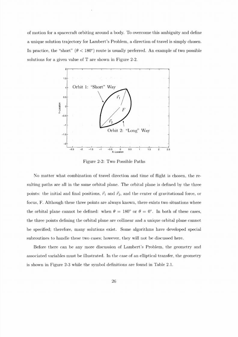
of motion for a spacecraft orbiting around a body. To overcome this ambiguity and define
a unique solution trajectory for Lambert's Problem, a direction of travel is simply chosen.
In practice, the "short" (0 < 180°) route is usually preferred. An example of two possible
solutions for a given value of 7l are shown in Figure 2-2.
c0
o
II
-2.5 -2 -1.5 -1 -0.5 0 0.5 1 1.5 2 2.5X-Location
Figure 2-2: Two Possible Paths
No matter what combination of travel direction and time of flight is chosen, the re-
sulting paths are all in the same orbital plane. The orbital plane is defined by the three
points: the initial and final positions, fr and r2, and the center of gravitational force, or
focus, F. Although these three points are always known, there exists two situations where
the orbital plane cannot be defined: when 0 = 180° or 0 = 0°. In both of these cases,
the three points defining the orbital plane are collinear and a unique orbital plane cannot
be specified; therefore, many solutions exist. Some algorithms have developed special
subroutines to handle these two cases; however, they will not be discussed here.
Before there can be any more discussion of Lambert's Problem, the geometry and
associated variables must be illustrated. In the case of an elliptical transfer, the geometry
is shown in Figure 2-3 while the symbol definitions are found in Table 2.1.
26

8/13/2019 Lambert Guidance
http://slidepdf.com/reader/full/lambert-guidance 27/122
a
Figure 2-3: Elliptical Transfer
Table 2.1: Symbol Definition
Symbol Definition
r- Starting Position Vector
r-2 Destination Position Vector0 Transfer angle
a Semi-major axis
c Chord
p Semiparameter
s Semiperimeter
e Eccentricity
El Eccentric Anomaly of Fr
E2 Eccentric Anomaly of 2
fi True Anomaly of r
f2 True Anomaly of r'i1i Velocity at i
i/72 Velocity at r2
In addition, similar drawings can be made for parabolic and hyperbolic transfers, which
can be found in Appendix A. More information about the derivation of these quantities
and their meanings can be found in several references, but most notably in Reference [2].
27

8/13/2019 Lambert Guidance
http://slidepdf.com/reader/full/lambert-guidance 28/122
2.1.2 Governing Equations
To solve Lambert's Problem, all of the values in Table 2.1 must be found to fully describe
the orbit and find the correlated velocity. After the path, either "short" or "long", has
been chosen, some quantities are found simply from the geometry, i.e.
= arccos (r 2 (2.2)
c= r2 2 2r r2cos (2.3)
rl + r 2+ Cs = - 2 (2.4)
The other quantities must be described in terms of the given quantities, ri, 2, T, and
those found from the geometry, 0, s, and c. The equations that describe the rest of the
quantities were developed by Lagrange after Lambert theorized that, "the orbital transfer
time () depends only upon the semimajor axis (a), the sum of the distances of the
initial and final points of the arc from the center of force (r1 + r2 ), and the length of the
chord joining these points (c)" [2]. Lagrange was the first to supply the analytic formulas
to prove Lambert's theories; therefore, these formulas are called Lagrange's Equations
and are stated in Equations 2.5-2.9 for an elliptic transfer. The Lagrange Equations for
parabolic and hyperbolic orbits are, again, listed in Appendix A. The two quantities ¥,
and cos were defined to simplify the set of equations (2.7-2.9).
1
-= (E2-E1l) (2.5)2
1cos=
ecos (E1 + E
2) (2.6)
2
= 2a2 (V1 sin cos ) (2.7)
r1 + r2 = 2a(1 - cos cos ) (2.8)
rr 2 cos- 0 = a(cos4' cos ) (2.9)2
28

8/13/2019 Lambert Guidance
http://slidepdf.com/reader/full/lambert-guidance 29/122
As can be seen by this set of equations, there are three equations and three unknowns:
a, , and . The methods of solving this set of equations is the subject of section
.2.1.3; however, once a solution is found, the other quantities listed in Table 2.1 can be
ascertained from Equations 2.10 and 2.11 for the elliptic transfer.
rl'r2sin 2osin- 2 (2.10)
a sin '
eC=/-- i(2.11)a
By finding '?, 0, a, p, and e, the unique orbit is completely defined, but the correlated
velocity still needs to be found. This is where another part of Lagrange's work is used.
Lagrange Coefficients, or F and G functions, are usually used in the form shown in
Equations 2.12 and 2.13. In this form, the position and velocity, Fr and i72,of a point
anywhere on the orbit can be found by knowing the position and velocity of another
point on the same orbit, where F, G, , and G are constants defined by the unique
transfer orbit. These equations are mainly used to propagate the position and velocity of
cl spacecraft on an orbit.
2 = F£~ + Gl (2.12)
i'2= FrF + Gi7l (2.13)
With some careful manipulation, the velocities at two points on an orbit, Ui and r2, can
be found given the two corresponding positions on that orbit, r' and r'2.
r-- F2t~l= ,G (2.14)
Gf¥ - r15 -2 (2.15)
In the case of Lambert's Problem, the correlated velocity is found by solving for iU in
29

8/13/2019 Lambert Guidance
http://slidepdf.com/reader/full/lambert-guidance 30/122
Equation 2.14. The quantities F, G, F, and G for elliptic orbits are found from Equations
2.16-2.19. Appendix A lists the Lagrange Coefficients for the Parabolic and Hyperbolic
cases.
F = 1- 2(1- cos) = 1 -(1 - cosT) (2.16)P rl
G = r2 r1 sin = '- f( sin ) (2.17)
F= / tan -cos _ 1 _ :- =- sin (2.18)p 2 p rl r rlr2
G1- (1 - cos) = 1- (1 - cos) (2.19)
The Lagrange Coefficients can also be used to solve Lambert's Problem without first
using Lagrange's Equations. As it turns out, F, G, F, and G, are not independent,
because they are described by only three unknowns: p, a, and A. Therefore, three of
the equations can be solved for the three unknowns and fully describe the unique orbit
between r'1 and r 2.
The derivation of the Lagrange Equations can be found in Reference [2] while the
derivation of the Lagrange Coefficients is shown in Reference [1].
2.1.3 Solution Techniques
Upon closer inspection of these two sets of three equations (2.7-2.9 and 2.16-2.18) no
amount of algebraic operations can analytically solve either set of equations for all three
unknowns, which means the they are transcendental and must be solve iteratively. This
property of the problem along with the importance of solving Lambert's Problem to the
study of Astrodynamics is what has spurred the development of several algorithms to solve
Lambert's Problem. Creating algorithms to iteratively find a solution has commanded
attention from scholars since Lambert first published his solution almost 250 years ago.
From Lambert's original solution to many algorithms developed by commercial companies
30
8/13/2019 Lambert Guidance
http://slidepdf.com/reader/full/lambert-guidance 31/122
and the military, there are a plethora of papers and documentation on how to solve this
problem.
While these algorithms were developed for varying reasons, their methods are all sim-
ilar: they choose an independent iteration parameter and either Lagrange's Equations or
Lagrange's Coefficients to solve for the unique solution orbit, then solve for the correlated
velocity.
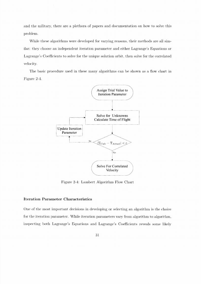
The basic procedure used in these many algorithms can be shown as a flow chart in
Figure 2-4.
Assign Trial Value to
Iteration Parameter
Figure 2-4: Lambert Algorithm Flow Chart
Iteration Parameter Characteristics
()he of the most important decisions in developing or selecting an algorithm is the choice
for the iteration parameter. While iteration parameters vary from algorithm to algorithm,
inspecting both Lagrange's Equations and Lagrange's Coefficients reveals some likely
31

8/13/2019 Lambert Guidance
http://slidepdf.com/reader/full/lambert-guidance 32/122
candidates for the iteration parameter, i.e. p, a, , and 4'. In addition, other quantities
have been utilized such as fl, the true anomaly and e, the eccentricity. These quantities
have also been transformed into other forms such as W2' or sin2 V4. Essentially any
quantity can be used as long as it either directly or indirectly involves one of the three
unknowns in the set of chosen equations.
Although any of these quantities can be chosen and used to solve Lambert's Problem,
some have characteristics that make them less desirable while others have advantageous
qualities, which must be taken into consideration when looking at an algorithm. For in-
stance, a has many characteristics associated with it that make it an unattractive iteration
parameter candidate. The time of flight equation (2.7) is a double-value function of a, so
a goes to infinity for a parabolic orbit, which may cause computational errors in an algo-
rithm. Furthermore, there are issues with other parameters such as p because according
to Battin in Reference [2] the semiparameter has the same value for all orbits in a 180°
transfer orbit, which in some cases may cause erroneous results. By choosing the true
anomaly as an iteration parameter, a singularity or multiple solutions when 0 = 180° can
be avoided, yet the orbital plane can still not be defined as stated previously in Section
2.1.1.
An important characteristic of an iteration parameter is its versatility. Throughout the
discussion of solving Lambert's Problem, it has been noted that there are three different
variations of both the Lagrange Equations and Lagrange Coefficients, one for each of the
elliptic, parabolic, and hyperbolic transfer orbit cases. It would be useful to have an
iteration parameter that is versatile and would encompass all possible orbits.
Some candidate iteration parameters that are defined for all orbits are the eccentricity,
true anomaly, and semiparameter. Furthermore, there are a host of other iteration pa-
rameters that are defined in terms of the eccentric, parabolic, and hyperbolic anomalies.
Based on the algorithms developed in References [2] and [8], the iteration parameters that
use the anomalies are developed using the difference between the anomaly values at the
32

8/13/2019 Lambert Guidance
http://slidepdf.com/reader/full/lambert-guidance 33/122
two positions. Therefore the actual iteration parameter ends up being AE, A/, and AH.
Where AE is tlhe change in eccentric anomaly, AO is the change ill parabolic anomaly,
and AH is the change in hyperbolic anomaly.
A = (E2 - E) (2.20)
zAx ( - 31)
AH = (H2 - H)
(2.21)
(2.22)
One iteration parameter that uses the anomaly differences is X as seen in Equation 2.23.
AE2
elliptic
0 parabolic
AH
2
(2.23)
hyberbolic
By definition E, > El and H2 > H1, hence the range of values for X can vary from
positive to negative with no discontinuities. Furthermore, values of X greater than zero
corresplond to ellipses, while values less than zero are hyperbolas and a value equal to zero
represents a parabolic orbit.
Other sets of iteration parameters that also have this property are X and .r defined
in Equations 2.24 and 2.25.
sin2 (AE)
0
-_ inh (AH)
tan2 (AE)
0
- tanh 2 (AH)4\~1
elliptic
parabolic
hyperbolic
elliptic
parabolic
hyperbolic
(2.24)
(2.25)
33

8/13/2019 Lambert Guidance
http://slidepdf.com/reader/full/lambert-guidance 34/122
2.2 Lambert Guidance
For any moment in time, the spacecraft's position and velocity, R and VR, are known and
the correlated velocity, fL, that satisfies the Lambert Problem can be found as described
in the previous section. Therefore, to get the spacecraft on the transfer trajectory found
from Lambert's Problem, a change in velocity () is needed. This Av' will be referred
to as the velocity-to-be-gained () and can be found from Equation 2.26.
VG = VL - VR (2.26)
A vector diagram of the relationship between iR, VL, and VG is shown in Figure 2-5.
VG
Figure 2-5: Lambert Guidance Vector Diagram
Once VG is calculated, it is fed into a steering algorithm, which has its own logic to
manipulate the thrust to reduce 'vG over time.
34

8/13/2019 Lambert Guidance
http://slidepdf.com/reader/full/lambert-guidance 35/122
Chapter 3
Rendezvous Problem
From the discussion in Chapter 2, a thrusting spacecraft can be steered, using Lambert
Guidance, from an initial position to a point where the engines can be shut off and the
spacecraft will coast to its final destination. One particular application where Lambert
Guidance can be used is that of the intercept problem. Whether it is an Earth-launched
ballistic missile intercepting a target on the ground, having one spacecraft performing a
fly-by inspection of another, or any of the other possible missions, vehicles using Lambert
Guidance for intercept missions have been successful.
To get a better understanding of an intercept problem, the fly-by inspection scenario
i.; outlined and a diagram of the mission is shown in Figure 3-1. For this mission, the
'Inspector" spacecraft, or chaser, on an initial orbit would execute a single manoeuver
burn using a Lambert Guidance Algorithm to get onto a transfer trajectory that reaches
the target point. Once 'G has been reduced to the cut-off value, the thrust terminates
and the chaser coasts the rest of the way to target point on the transfer trajectory. Onceat the target point, the fly-by inspection occurs and the chaser continues on the transfer
orbit while the "'Target" continues on its original orbit. Although the two spacecraft get
il:L lose proximity, their velocities at the target point are such that their positions diverge
soon after their closest encounter.
35

8/13/2019 Lambert Guidance
http://slidepdf.com/reader/full/lambert-guidance 36/122
-- Chaser's Position After InterceptTarget's Position After Intercept
*Not to Scale Chaser's Original Orbit
Figure 3-1: Intercept Diagram
While a Lambert Guidance Algorithm is well-suited for intercept problems, it does
not have direct control over the spacecraft's velocity when it gets to the target point;
therefore, applications such as rendezvous, which require a specific velocity at the target
point, must either use a different guidance algorithm, or use a modified Lambert Guidance
Algorithm.
The development of a particular method to modify a Lambert Guidance Algorithm
(LGA) to create an Augmented Lambert Guidance Algorithm (ALGA) is discussed in
detail in Chapter 4; however, the rendezvous problem description, including assumptions
and success criteria, is the subject of this chapter.
3.1 Problem Definition
Figure 3-2 shows a typical trajectory for the rendezvous missions discussed in this thesis.
A launch vehicle, initially at rest on the surface of the Earth, launches off its platform and
performs the first burn, which is referred to as the boost phase. The engine is then cut
off and the vehicle coasts on the transfer trajectory. Some time later, the chaser performs
36

8/13/2019 Lambert Guidance
http://slidepdf.com/reader/full/lambert-guidance 37/122
a secon(l burn inanoeuver to match both the position and velocity of the orbiting target
spacecraft. The target and chaser follow the same orbit after the second burn until a time
when the terminal manoeuvres for inspection and/or docking are performed.
Burn 2
/,Target and Chaser
Follow Same Orbit
*Not to Sca
*
fer Trajectory
(Coast)
Figure 3-2: Rendezvous Diagram
3.2 Assumptions
Be ore the process of designing the ALGA could commence, assumptions were made to
provide a framework from which to develop the algorithm. These assumptions dictate the
dynamic equations used along with the initial conditions and vehicle configuration used
to further characterize how to create the ALGA.
3.2.1 Initial and Target Conditions
At the launch tin-Le,he chaser knows all of its physical characteristics, i.e. weight, number
of stages, etc. along with its position on the globe perfectly and is at rest at the surface
37

8/13/2019 Lambert Guidance
http://slidepdf.com/reader/full/lambert-guidance 38/122
of the Earth.
R (0) = 'o (3.1)
fR(0) = (3.2)
Additionally, the chaser is given the exact position and velocity of the target spacecraft
at the launch time along with the time of flight to the target, 'T.
r--/c(O) .=s/co (3.3)
Vs /c(O) = es/c0 (3.4)
The target spacecraft is designated as a non-manoeuvering target; therefore, its path is
an orbit around the Earth. Given the initial conditions and the specification that it moves
in a predictable orbit, the position and velocity (r/c and v%/,)of the target spacecraft can
be found by propagating the initial conditions along the orbit over a time interval using
Lagrange Coefficients. The target conditions are then found from Equations 3.5 and 3.6.
fT = f,/c((T) (3.5)
lvT = X/c(T) (3.6)
3.2.2 Dynamics
One major assumption is that all of the motion is governed by the two-body approxima-
tion. This assumption provides sufficient accuracy to perform a first-order evaluation of
the ALGA and significantly simplifies the necessary equations.
In combination with the two-body approximation, the target spacecraft and chaser's
motion will be found with respect to the Earth, which will be modeled as a non-rotating,
perfect sphere with gravity being proportional to the square of the distance from the
38

8/13/2019 Lambert Guidance
http://slidepdf.com/reader/full/lambert-guidance 39/122
center of the Earth as described by Newton's Second Law.
Although effects from the oblateness of the earth, atmospheric drag, solar radiation
pressure and third-body gravitation would perturb the actual trajectory of the vehicles,
they will be neglected for this analysis.
3.2.3 Vehicle
For the rendezvous mission scenarios to be investigated in this thesis, the target spacecraft
was elected to be launched from the surface of the Earth on either a land- or sea-based
platform. The vehicle is assumed to have multiple stages to bring a payload to orbit;
therefore, the chaser will consist of three boost stages and the payload.
As stated before, the LGA has no direct control over the velocity of a spacecraft
when it gets to its destination. A second burn provides the necessary velocity change
needed to match both the position and velocity of the target spacecraft. To execute
this manoeuver, the spacecraft payload must have a motor and fuel available to achieve
the second manoeuver. Hence, the payload will consist of an additional 4 th stage engine
attached to the 100 kg structure and equipment (i.e., cameras, sensors, etc.) essential to
the mission.
The second burn, also known as the 4 th stage manoeuver, was chosen to have a constant
thrust magnitude and a fixed thrust direction with respect to the Earth for the entire burn
tinie, Tb. The 4t" stage ignites at a time, 7' 4 th, SO hat after the 4th stage burn the chaser
can terminate its thrust and arrive at the target point at the given time, ¶'.
74t =F - b (3.7)
Dictated by the amount of velocity change needed to rendezvous with the target, b, and
therefore 7Tl4 th, are both variable quantities. Consequently, the 4 th stage is assumed to be
able to initiate and terminate its thrust according to these values. Tile chaser can begin
39
8/13/2019 Lambert Guidance
http://slidepdf.com/reader/full/lambert-guidance 40/122
its terminal guidance either immediately after the 4 th stage cut-off or at any future time.
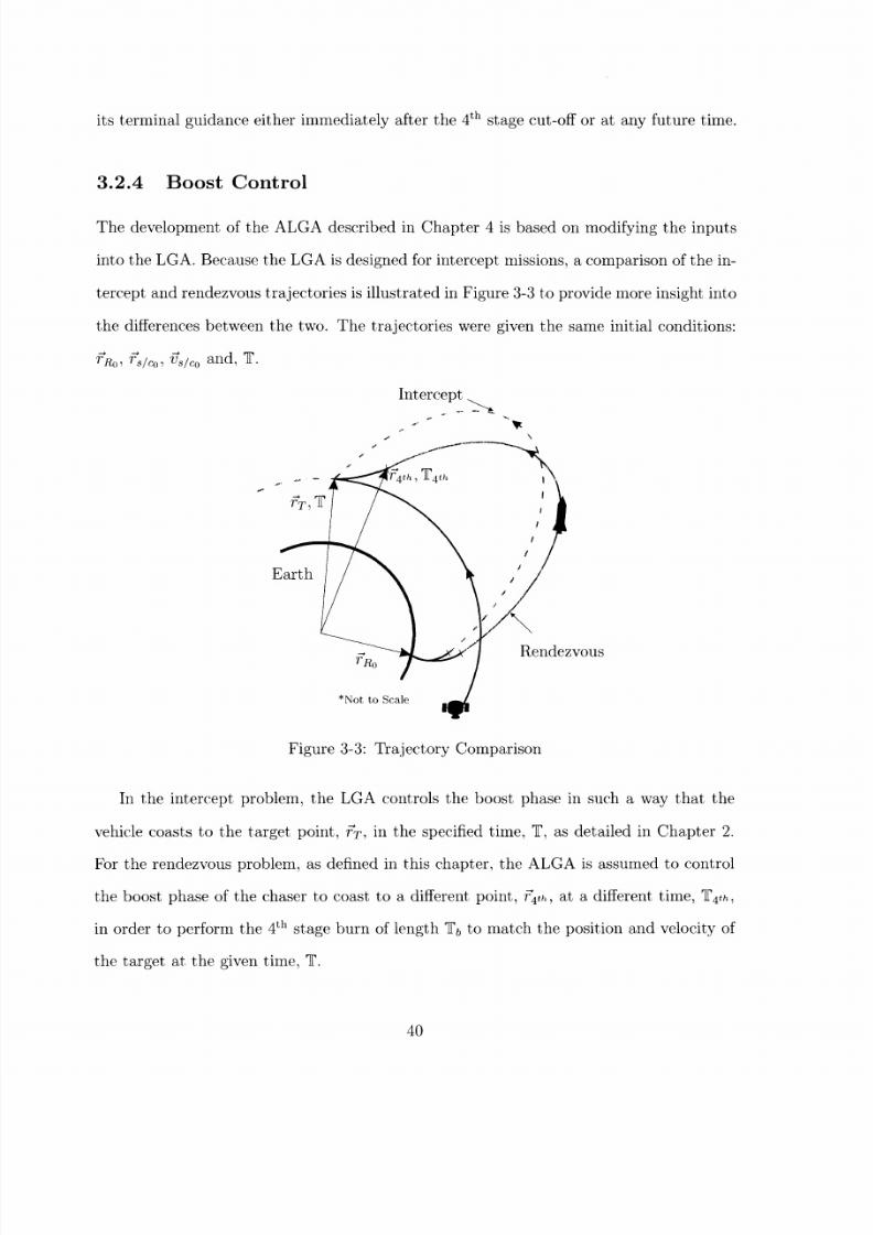
3.2.4 Boost Control
The development of the ALGA described in Chapter 4 is based on modifying the inputs
into the LGA. Because the LGA is designed for intercept missions, a comparison of the in-
tercept and rendezvous trajectories is illustrated in Figure 3-3 to provide more insight into
the differences between the two. The trajectories were given the same initial conditions:
TRo, rs/co, vs/co and, T.
Intercept
ZVOUS
Figure 3-3: Trajectory Comparison
In the intercept problem, the LGA controls the boost phase in such a way that the
vehicle coasts to the target point, rT, in the specified time, ¶', as detailed in Chapter 2.
For the rendezvous problem, as defined in this chapter, the ALGA is assumed to control
the boost phase of the chaser to coast to a different point, i4th, at a different time, 'l 4 th,
in order to perform the 4 th stage burn of length Tb to match the position and velocity of
the target at the given time, 7.
40

8/13/2019 Lambert Guidance
http://slidepdf.com/reader/full/lambert-guidance 41/122

8/13/2019 Lambert Guidance
http://slidepdf.com/reader/full/lambert-guidance 42/122
Delta II - Developed mainly to launch US Air Force payloads into GPS or LEO orbits,
the Delta II is available in two- and three-stage versions (with a zeroth solid rocket
booster stage) to accommodate both small and medium payloads. The first and
second stages are liquid fueled and the optional third stage is solid fueled.
Minotaur - Used by the US Air Force, this launch vehicle combines parts from the
Minuteman II ICBM and Pegasus XL launch vehicle (Made by The Orbital Sciences
Corporation) to launch small payloads into LEO orbits. Its four stages are solid
fueled.
Taurus - This solid fueled four-stage launch vehicle originally used a Peacekeeper missile
for the first stage and a Pegasus as an upper stage to launch military payloads.
Then The Orbital Sciences Corporation used a commercial first stage to create a
commercial version and launch small payloads into LEO and GTO.
Boost Sizing
The vehicle design specification values for the Space Launch Systems described previously,
again gathered from Reference [7], were tabulated in a spreadsheet and then averaged.
The tabulated data from Reference [7] can be found in Appendix B. Using engineering
judgement, values were then chosen for the specific quantities needed for the boost stages.
The following table describes the specifications of the chosen chaser to be used in the
simulation.
Table 3.1: Boost Stage Specifications
Engine Statistics MassStage Thrust Burn Time ISP Structural Propellant Fraction
Newtons Seconds Seconds Kg Kg unitless
1 1,409,250 78.05 258.10 4276.50 45221.25 0.91
2 746,600 70.46 278.50 2141.00 20496.80 0.91
3 186,200 95.52 289.24 794.25 6143.00 0.89
42
8/13/2019 Lambert Guidance
http://slidepdf.com/reader/full/lambert-guidance 43/122
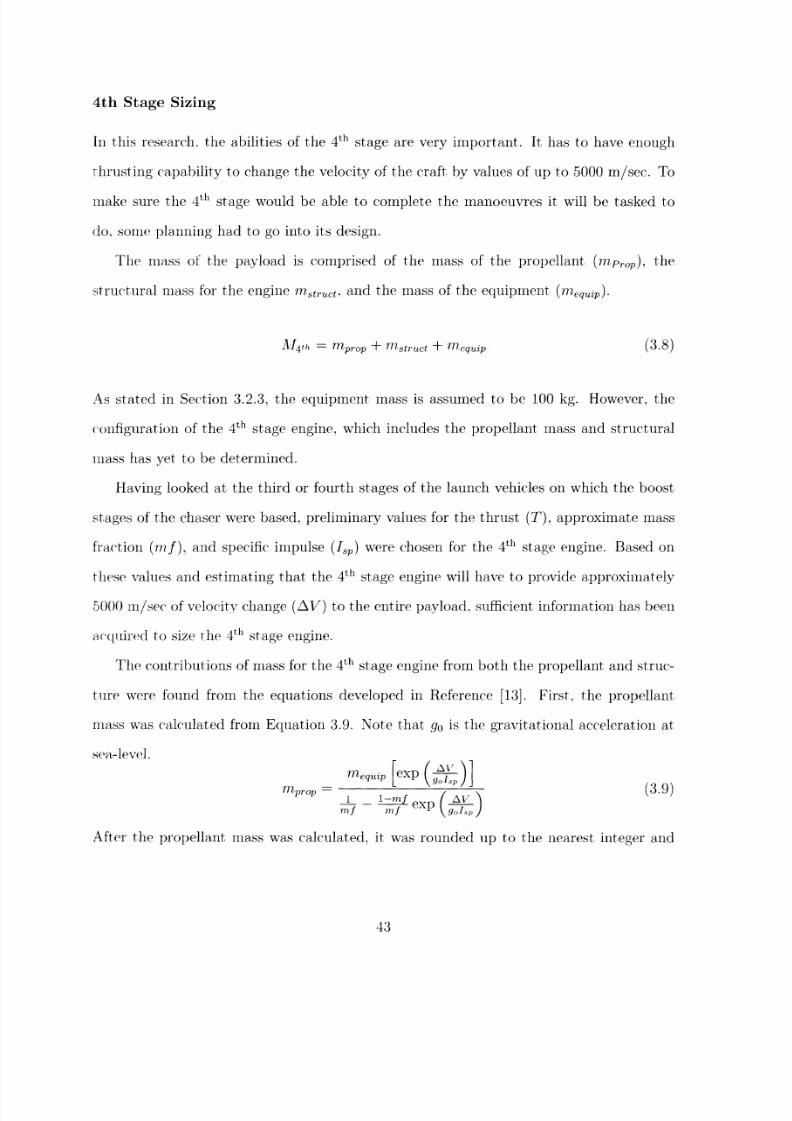
4th Stage Sizing
[In his research, the abilities of the 4 th stage are very important. It has to have enough
1hrusting capability to change the velocity of the craft by values of up to 5000 m/sec. To
make sure the 4th stage would be able to complete the manoeuvres it will be tasked to
do, some planning had to go into its design.
The mass of the payload is comprised of the mass of the propellant (m'prp), the
structural mass for the engine mnt,r,,t, and the mass of the equipment (mequip).
A'Ith = mprop + Mstruct + me quip (3.8)
As stated in Section 3.2.3, the equipment mass is assumed to be 100 kg. However, the
configuration of the 4th stage engine, which includes the propellant mass and structural
mass has yet to be determined.
Having looked at the third or fourth stages of the launch vehicles on which the boost
stages of the chaser were based, preliminary values for the thrust (T), approximate mass
fraction (f), and specific impulse (Ip) were chosen for the 4 th stage engine. Based on
these values and estimating that the 4 th stage engine will have to provide approximately
5000 m/sec of velocity change (AV) to the entire payload, sufficient information has been
acqluired to size he 4 stage engine.
The contributions of mass for the 4th stage engine from both the propellant and struc-
ture were found from the equations developed in Reference [13]. First, the propellant
mass was calculated from Equation 3.9. Note that go is the gravitational acceleration at
sea-level.mequi [exp (g),I,p
Aeprop All (3.9)f1 emfxpAV
After the propellant nmasswas calculated, it was rounded up to the nearest integer and
43

8/13/2019 Lambert Guidance
http://slidepdf.com/reader/full/lambert-guidance 44/122
Equation 3.10 is then used to find the structural mass.
mtprop(1m f) (3.10)istruct m f
mf
As a consequence of having a limited amount of fuel, there is a finite amount of time
in which the 4 th stage engine can burn fuel and produce thrust. Given the propellant
mass, the maximum burn time was calculated from Equation 3.11.
Ispgomrprop (3.11)bmax-- T
After all of the calculations, the 4 th stage engine specifications are now known and are
shown in Table 3.2.
Table 3.2: 4th Stage Engine Specifications
Engine Statistics Mass
Stage Thrust Burn Time ISP Structural Propellant FractionNewtons Seconds Seconds Kg Kg unitless
4 10,000 264.87 300 100 900 0.90
3.3.2 Target Orbits
Based on the capabilities of the US Space Launch Systems, it is impractical to try and
rendezvous with a target spacecraft in such a high altitude orbit as a geostationary com-
munications satellite, because the Space Launch Systems simply do not have enough fuel
to reach those high altitude orbits. Therefore, the possible orbits for the target spacecraft
are limited to Low Earth Orbits (LEO), which are defined as orbits whose semimajor axis
is between 100km and 500km greater than the radius of the Earth.
Because of the limited fuel, the chaser launch vehicle is presumed to not have enough
fuel to reach the parabolic and hyperbolic escape velocities; consequently, the focus is
primarily on circular and elliptic target orbits.
44

8/13/2019 Lambert Guidance
http://slidepdf.com/reader/full/lambert-guidance 45/122
3.4 Success Criteria
After the development of the ALGA, it must be tested for its effectiveness. To this end,
computer models are created to replicate the conditions of an actual test flight. Test.cases
are constructed that utilize various initial conditions for the chaser and an assortment of
target orbits, which adhere to the requirements outlined previously. The information
gene]rated by the test cases is used as inputs to the Simulink simulation software, which
executes the logic dictated by the models over the given time interval, ¶'. The models
used in the simulation to test the ALGA are described in Chapter 5.
At the completion of the simulation, the effectiveness of the ALGA in guiding the
chaser to rendezvous with the target can be evaluated for that particular test case. The
evaluation is based on four factors. Two of the factors are based on calculating the
deviation in the position and velocity of the chaser with respect to the target. The
position and velocity errors, Rer and Ve,, respectively, are defined as the magnitude
difference between the value for the chaser and the value for the target spacecraft at the
rendezvous time. 1'.
Re,, = l R - /cl (3.12)
Verr fjR - Us/cI (3.13)
A. test case is deemed successful if the following four criteria are met:
1. The chaser does not impact the Earth - The magnitude of the chaser's position
vector (R) is never less than the radius of the Earth (r).
rR > re (3.14)
2. The 4 h stage does not run out of fuel - The burn time needed to perform the
45

8/13/2019 Lambert Guidance
http://slidepdf.com/reader/full/lambert-guidance 46/122
rendezvous does not exceed the maximum burn time of the 4 th stage.
(3.15)b < bmax
3. The Position Error is within tolerable limits - The value is less than 100 meters.
Rerr < 100 m (3.16)
4. The Velocity Error is within tolerable limits - The value is less than 0.5 me-
ters/second.
Verr < 0.5 m/sec (3.17)
46

8/13/2019 Lambert Guidance
http://slidepdf.com/reader/full/lambert-guidance 47/122
Chapter 4
Augmenting Lambert
Starting with a preexisting Lambert Guidance Algorithm (LGA) in conjunction with
the assumptions outlined in Chapter 3, a method was devised to create the Augmented
Lambert Guidance Algorithm (ALGA) for use in rendezvous missions. This method
entails the creation of an adjunct algorithm that modifies the inputs into the original LGA
as opposed to explicitly altering it. The inspiration for creating an adjunct algorithm that
utilizes the given LGA stems from the implementation in an actual launch vehicle. The
adjunct algorithm could be placed on a supplementary processor or as a separate function
within the existing guidance algorithm processor. Essentially, the adjunct algorithm could
be se(l as an optional module that could be added based on the rmission requirements.
Tihe general procedure used to generate the ALGA is derived from the work done by
Burns and Scherock as described in Reference [6]. In their analysis, they ignored the
effects of the changing gravity vector during the 4 th stage burn because their chaser and
target were both traveling on ballistic trajectories and their burn times were relativelyshort (<50 seconds). In contrast, the missions discussed in this thesis have the target in an
orbital trajectory and the burn times are anticipated to be long (100-300 seconds) due to
tllhe arge ANi hanges (maximum of 5000 m/sec). Therefore, ignoring the shifting gravity
vector could not be upheld for the analysis in this thesis. Consequently, the method
47

8/13/2019 Lambert Guidance
http://slidepdf.com/reader/full/lambert-guidance 48/122
derived in this chapter builds upon the technique created by Burns and Scherock. This
new method provides insight into how to modify the inputs to the LGA while including
compensation for the varying gravity vector during the 4 th stage burn.
4.1 General Procedure
As stated in Chapter 3, the objective of the ALGA is to get the chaser on a transfer tra-
jectory that reaches r4that the time 7 4 th. It is then the adjunct algorithm's task to modify
the inputs given to the LGA to produce the expected transfer trajectory. Considering
what values the LGA needs to compute vcG, the adjunct algorithm is only able to modify
the target position, T, the current position, rR, and/or the time of flight, T7,given to the
LGA. Consequently, there are seven possible combinations of modified inputs that could
be given to the LGA and produce the same transfer trajectory.
1. Modify only the target position. INPUTS: fiTmod, 7, and ¥R
2. Modify only the time of flight. INPUTS: , ,,mod, and r
3. Modify only the current position. INPUTS: r, T, and 'RRmod
4. Modify the target position and the time of flight. INPUTS: ¥Tmod, Tmod, and ¥R
5. Modify the target position and the current position. INPUTS: Tmod, 7, and rRmod
6. Modify the time of flight and the current position. INPUTS: , mo,,d and irRmod
7. Modify all three inputs. INPUTS: 'iTmod, 7Tmod,and ¥rRmod
In this thesis, the choice was made to implement option one, thereby only modifying
one input into the LGA; the target position, T. Figure 4-1 shows the relationship between
the actual target point, modified target position, and the ignition point; T, Tmod,and
'r4th, respectively.
48

8/13/2019 Lambert Guidance
http://slidepdf.com/reader/full/lambert-guidance 49/122
I
Zvous
Figure 4-1: False Target Diagram
By fixing the time of flight, several properties of the modified target position become
evident. First, as a result of the 4th stage burn, the chaser never reaches FrTmod providing
the 4t11 tage engine ignites); so, an important characteristic of rTTmod s that it is a false
target. Another feature of this point is that the time to get from f'4tho rTmod is equal to
the time to get from 4 th to T, which is the burn time, T b.
Calculating r;)mod requires that the chaser reach rt th at I'4 th; hence, it would be helpful
to know those values. However, 4th and T 4 th are dependant on the values of the thrust
direction vector, B 1L, and the burn time, 7Tb.Both of these values are initially unknown
and are, coincidentally, needed by the other systems on the chaser to successfully exe-
c-ute the 4th stage nanoeuver. Therefore, in addition to calculating rTmod, the adjunct
algorithm is also responsible for calculating Tb and B 4 th.
The goal of the adjunct algorithm as part of the ALGA is to exploit the properties of
the LGA and the methods used by Burns and Scherock to calculate the three unknown
Values: Trnod,l B41 th, and Tb. The modified technique is outlined in Figure 4-2. As can be
seen from the flow chart, there are five main steps (shown by bold outline): Initialization,
St-ate Propagation, Match Velocity, Match Position, and Iteration.
49

8/13/2019 Lambert Guidance
http://slidepdf.com/reader/full/lambert-guidance 50/122
Figure 4-2: ALGA Flow Diagram
The Initialization block employs the method used by Burns and Scherock to find initial
approximations for the three unknowns. Therefore, the initialization values are found by
50

8/13/2019 Lambert Guidance
http://slidepdf.com/reader/full/lambert-guidance 51/122
nLeglecting he change in the acceleration due to gravity while the 4th stage engine is
thrusting. The LGA is run using either the quantities from the Initialization block or
the values from the previous time step depending on whether this is the first time the
ALGA is called. The state produced by the LGA is propagated forward to get values at
the rendezvous time in the State Propagation block. These terminal conditions are then
used by the Match Position and NMatchVelocity blocks to generate updated values for the
unknowns. The Matching Position block produces a more accurate value of ¥Tmodwhile
the Matching Velocity block updates the values for B 4 th and 7b. The outputs of these two
blocks collectively compensate for the effects due to the variation in gravity during the
4 th stage burn. Finally, an outer iteration loop is used to produce more accurate values
for r-7'od, 4th, alnd Tb.
z4.2 Initialization
On the first call to the ALGA, the only information given is the initial conditions as
described in Section 3.2.1. The goal of the initialization block is to take the initial con-
ditions and produce reasonable approximations for the three unknowns. This is done by
making a first guess for the three unknowns, propagating the chaser's state forward to
findllhe terminal conditions, then updating the values for the three unknowns based on
the assumption that the gravity vector during the 4 th stage burn doesn't change.
4.2.1 First Guess
The first-guess step entails setting the 4 th stage burn time to zero and the modified target
position equal to the actual target position and running these values through the LGA.
7b = 0 (4.1)
'rTmod= T (4.2)
51

8/13/2019 Lambert Guidance
http://slidepdf.com/reader/full/lambert-guidance 52/122
By setting these initial conditions, the resulting output from the LGA is essentially the
correlated velocity needed to be on an intercept trajectory to the target.
4.2.2 Propagation
Using the current chaser position, and the correlated velocity computed by the LGA, the
chaser's position and velocity are propagated forward in time by rITo define the terminal
conditions of the initialization trajectory. The propagation is accomplished using the
Lagrange Coefficients method mentioned in Section 2.1.1. To find more information on
using the Lagrange Coefficients to propagate a spacecraft's trajectory, see References [2]
and [11].
The terminal conditions defined by the propagation of the initialization trajectory gives
the chaser's velocity, R, at the actual target point, T, and provides the adjunct algorithm
with a starting point from which to begin its calculations for the three unknowns.
Figure 4-3 is the area highlighted in Figure 4-1 and illustrates the initialization tra-
jectory along with the chaser's velocity and the target spacecraft's velocity at the actual
target point.
InitializationTrajectory
Figure 4-3: Rendezvous Velocity Vectors
52

8/13/2019 Lambert Guidance
http://slidepdf.com/reader/full/lambert-guidance 53/122
4.2.3 Thrust Direction
iAs can be seen from the figure, Ai7 is the relative change in velocity that needs to occur
to make the velocities of the chaser and target match, which is the reason for the 4 th stage
burn. The initial value of Ai7 is found from Equation 4.3.
At = v/c- 'R (4.3)
Once a value for Ai7 has been found, the next step in the initialization is to find the
thrust direction required to reduce Ai7 to zero by the rendezvous time, T'. To do this,
the chaser initiates a 4 th stage manoeuver at 4th in the direction of B4th. By aligningI:,Ith with Ait, 2iRchanges over time and constantly reduces Ai. Reducing AiYt o zero
accomplishes the goal of matching the velocity. The 4 thstage thrust direction vector B4 th
is then defined by a unit vector in the direction of At. As it turns out, the magnitude of
Ak5 as well as its direction is needed in future calculations; therefore, Ai7 will be passed
out of the Initialization block and B4th will be extracted from that value when needed.
4.2.4 Burn Time
Rmemnlbering that 'l4t1, s calculated by subtracting b fom ' (Equation 3.7). the value
of b is a reasonable choice for the next unknown to be calculated.
The thrust provided by the 4 th stage engine is used to reduce Ai7 to zero over the burn
time, b. Therefore, Al5 can be calculated by integrating the acceleration experienced by
the chaser over the same interval.
Ae= i R(t) dt (4.4)
Given that the 4th stage provides a constant thrust and burns its fuel at a constant rate,
AJ, where Mo4th is the initial mass of the 4thstage, the acceleration due to thrust can be
53

8/13/2019 Lambert Guidance
http://slidepdf.com/reader/full/lambert-guidance 54/122

8/13/2019 Lambert Guidance
http://slidepdf.com/reader/full/lambert-guidance 55/122
When the position offset is found, the modified target position can finally be calculated
from Equation 4.9
Tmod = rT - (4.9)
4.3 State Propagation
UJsing he burn time, modified target position, and thrust direction vector calculated from
Equations 4.7, 4.9, and 4.3 will result in the chaser not matching the position and velocity
of the target spacecraft due to the change in gravity vector during the burn. Figure 4-4
shows the gravity vectors when the 4th stage ignites and at the target point along with
its effect on the chaser during the burn.
94th
Figure 4-4: Gravity Vectors
Not, accounting for the variation in gravity results in the acceleration experienced by
the chaser, aR, being rotated. The amount of rotation is governed by how much the
gravity vector changes from the ignition point to the final position after the burn. This
change is denoted by Ag! in the figure. As a consequence of the rotating acceleration
vector, the position and velocity of the chaser also change direction and the chaser is
driven away from the desired target location as shown by the dotted trajectory.
The objective of the State Propagation block in conjunction with the Match Position
and Match Velocity blocks is to calculate values of B 4 th, Tmod, and T b that account for
55

8/13/2019 Lambert Guidance
http://slidepdf.com/reader/full/lambert-guidance 56/122
the change in gravity over the burn time.
To more accurately represent the dynamics, gravity is now included in the acceleration
equation experienced by the chaser and is shown in Equation 4.10.
aR = B4th R (4.10)[M4th glt
Unfortunately, this equation cannot be analytically integrated with respect to time
like Burns and Scherock were able to do for the acceleration when ignoring gravity. To
remedy this, a method was devised to account for the gravity variation.
First, the current chaser position along with the correlated velocity produced from the
call to the LGA is propagated forward using Lagrange Coefficients. This is identical to
the propagation done in the Initialization block in Section 4.2.2, except it is propagated
forward to the ignition time, 74th. The value of 74th is given by either the Initialization
block or the value from the previous iteration.
The second step involves using a separate fourth-order Runge-Kutta integrator to
numerically integrate Equation 4.10 over the burn time, b. The initial conditions given
to the Runge-Kutta integrator are the position and velocity output from the Lagrange
Coefficient propagation. The result of this second propagation is the predicted position, rp,
and velocity, /ip, of the chaser after coasting, executing the 4th stage burn and accounting
for the effects of gravity. From these predicted values, the position and velocity of the
target spacecraft are matched using the following techniques.
4.3.1 Matching Position
Figure 4-5 shows a possible miss-trajectory as predicted by the State Propagation block
using values for 7 4 th, irTmod, and Ai7 from either the Initialization block or from the
previous iteration.
To find a better value of rTmod,the difference in the predicted position and target
56

8/13/2019 Lambert Guidance
http://slidepdf.com/reader/full/lambert-guidance 57/122
Trnodfdp
Figure 4-5: Matching Position
spacecraft position is found.
rmiss = rp - rT (4.11)
This value for the miss distance is then subtracted from target position given to the LGA.
T,w = rTmod ¥rmiss (4.12)
A diagram of the vector addition is shown in Figure 4-6.
Figure 4-6: Matching Position Vector Addition
Once an updated value of FTneu,s calculated it is used as an input to the LGA to get
a new value of G. The State Propagation block is then executed again to acquire an
updated predicted position and miss distance. This procedure is repeated until the value
of FT_,, changes minimally over successive iterations. To find the appropriate number of
57
--- -- - - -- - - -- - -

8/13/2019 Lambert Guidance
http://slidepdf.com/reader/full/lambert-guidance 58/122
iterations, the magnitude of the miss distance versus the number of iterations was charted
for one call to ALGA and one set of initial conditions. Figure 4-7 shows a logarithmic
decrease in the magnitude of the miss distance over successive iterations. As can be seen
by this particular example, the predicted miss distance for the sixth iteration is on the
order of 10-6. Several other trajectories were examined and it was established that six
iterations leads to sufficient accuracy. Additionally, the three lines represent the three
outer loop iterations as shown in Figure 4-2 and discussed further in Section 4.4.
MatchPosition rror s. Iteration
2 3 4 5 6IterationNumber
7 8 9 10
Figure 4-7: Matching Position Error
4.3.2 Matching Velocity
Using the predicted velocity, p, from the Runge-Kutta integrator and Equations 4.6 and
4.7, an updated value for the thrust direction vector, B 4 th, and burn time, Tb, can be
calculated. This updated value, again, takes into account the velocity difference due to
gravity.
Figure 4-8 shows the predicted velocity with respect to the target spacecraft velocity
58
104
102
100
I-
10- 2L
0
a
.e
a.
-10
10- 4
10- 6
10- 8
_.
I_1[
I1

8/13/2019 Lambert Guidance
http://slidepdf.com/reader/full/lambert-guidance 59/122
aIlnd he value of' Af passed from the Initialization block or the previous time step, which
is parallel to the thrust direction vector, Bth.
s/c
Figure 4-8: Matching Velocity
The first calculation to find improved values for the thrust direction vector and burn
time is to take the difference between the predicted chaser velocity and target velocity.
miss = s/cl, lp (4.13)
This miss velocity is an additional change in velocity that the 4 th stage needs to provide
to the chaser to match the velocity of the target spacecraft. Therefore, the miss velocity
is added to the initial value of the velocity change, A&.
A/nnet,= Av + &miss (4.14)
Figure 4-9 shows a diagram of the vector addition used to calculate the new velocity
change.
The updated velocity change, AVw, is now a closer approximation to how much
velocity change the 4th stage needs to provide. Given that the thrust supplied by the
4.1 stage is constant, the burn time must be adjusted to accommodate the new velocity
change. Equation 4.15 is used to calculate the new burn time.
Tb new = LIth - exp () (4.15)
59

8/13/2019 Lambert Guidance
http://slidepdf.com/reader/full/lambert-guidance 60/122
Figure 4-9: Matching Velocity Vector Addition
4.4 Iteration
The techniques employed to update the values of Tmod, B 4 th and Tb did so by matching
the position and velocity separately. Because the position and velocity of the chaser are
coupled, an iteration scheme needs to be implemented to get increased accuracy for the
valuesof i¥Tmod, B4 th and Tb-
This can be seen by running the same initial condition, but only changing the number
of iterations used to calculate the three unknown values. Table 4.1 shows the difference
in Rerr and Verr when the number of iterations is increased from 2 to 3 for one particular
set of initial conditions.
Table 4.1: Rerr and Verrvs. Iterations
Iteration Rerr, (m) Verr (m/s)
1 30.5858 0.2686
2 51.5083 0.1422
3 10.0722 0.0798
Consequently, the number of iterations chosen for the ALGA used in this thesis is
three. This provides sufficient accuracy given the success criteria outlined in Section 3.4.
Once the three iterations are performed, the ALGA outputs Tmod, Tb, and AVi (re-
membering that B 4 th is the unit vector of AIf) to be saved and used in the next call to
ALGA at a future time step.
60
A,

8/13/2019 Lambert Guidance
http://slidepdf.com/reader/full/lambert-guidance 61/122
Chapter 5
Models & Simulation
Modeling and Simulation of physical systems has become an indispensable tool in evaluat-
ing and developing new algorithms, software, and hardware in not only the space industry,
but in every engineering field. Using such computer software as MATLAB, Simulink, and
functions written in C-code, several models were created to embody the physical charac-
teristics of the chaser, target spacecraft, and the environment in which they both operate.
Tile implementation of the logic contained in the models over time creates the computer
simulation, which will be used as a first-order assessment of the Augmented Lambert
Guidance Algorithm (ALGA) developed in Chapter 4.
After the logic and equations dictated by the models are integrated into the simulation
software, the robustness and versatility of the ALGA can be tested by running several
simulations with various initial conditions. The results of running multiple simulations are
used to gauge how successful the ALGA is at manoeuvering the chaser to rendezvous with
the target spacecraft. The success of the algorithm will be determined by how well it meetsthe criteria laid out in Chapter 3 and will be discussed comprehensively in Chapter 6. But
first, this chapter focuses on the logic and equations used to mimic the physical properties
of the two vehicles and the dynamics of motion. These equations define the models, which
are implemented using simulation software to create the computer simulation.
61

8/13/2019 Lambert Guidance
http://slidepdf.com/reader/full/lambert-guidance 62/122
5.1 Models
The simulation used to evaluate the ALGA includes four separate functional models whose
interactions are depicted in Figure 5-1. The current time measured from launch and the
remaining flight time is available in all of the models. The four models are described in
this chapter in conjunction with diagrams outlining their operations performed. These
models implement the assumptions outlined in Chapter 3.
Figure 5-1: Model Diagram
The Vehicle Staging Model encompasses the physical characteristics of the chaser, from
the mass depletion as a result of the burning of fiel to the execution of the stage separation.
The 3-DOF Vehicle Dynamics Model doubly integrates the accelerations experienced by
both the chaser and target spacecraft to provide the position and velocity of both vehicles.
The execution of the ALGA is contained in the Guidance Model, while the Steering Model
manages how the thrust of the chaser is directed throughout the trajectory from launch
to rendezvous.
5.1.1 Symbol Definition
Although most of the symbols used in the four functional models have been defined and
used throughout the preceding chapters, a table is included here as a refresher.
62

8/13/2019 Lambert Guidance
http://slidepdf.com/reader/full/lambert-guidance 63/122
Table 5.1: Model Symbols
Symbol DefinitionAIR Mass- Chaser
T Thrust- Chaser
B Steering Vector
r/Ic Position- Target
's/c Velocity- Target
iR Position- Chaser
i7'R Velocity- Chaser
/)Gc Velocity-to-be-GainedB 4th Thrust DirectionVector- 4 th Stage
14th Mass- 4 th StageTb Burn Time - 4th StageTsi Thrust - it h Stage
Alsi Mass - ith StageMlpay Mass- Payload
aT Acceleration- Thrust
aR Acceleration- Chaser
as/c Acceleration- Target
gR Gravity- Chaser
9/c Gravity- Target
5.1.2 Vehicle Staging Model
A generic small launch vehicle (GSLV), as discussed in Chapter 3, was chosen to be used as
the chaser in the simulation. The staging conditions for the GSLV have been implemented
to follow the vehicle model flow chart shown in Figure 5-2. A stage controller receives
cut-off signals from the Guidance Model, which it uses along with it's own logic to give
signals to each of the stage motor subsystems. These signals indicate when it is time to
either ignite the motor and begin expending fuel or to separate the remaining fuel and
structural mass from the vehicle. This controller is where the physical limitations of the
rocket stages are implemented. For instance, no two stages can be burning at the same
time and the current stage cannot ignite without having first deployed the previous stages.
Each of these stage motor subsystems controls a mechanism that computes the pro-
pellant rernaining in the storage tanks after the motor is given the signal to ignite. While
63

8/13/2019 Lambert Guidance
http://slidepdf.com/reader/full/lambert-guidance 64/122
the propellant mass is depleting, the model also outputs the thrust value produced by the
particular engine. When one motor is ignited, the thrust produced by the other stages
is zero. Furthermore, once a stage is separated it contributes values of zero for the mass
and thrust into the summations at the right of the diagram. To accurately represent the
chaser's thrust and mass characteristics at any time during the simulation, the thrust and
mass contributions from all of the stages is summed and output from the Vehicle Staging
Model.
I. I
cut-off si T
AIR
M 4th
L-…. _____________------- ____J
Figure 5-2: Vehicle Model Diagram
5.1.3 3-DOF Dynamics Model
Accurately describing the motion of the chaser relative to the Earth is critical to creating
a useful simulation. Based on the assumptions outlined in Chapter 3, the equation of
motion for the chaser and target are described by Equation 5.1.
dr+ r- aT = (5.1)dt2 r3
64

8/13/2019 Lambert Guidance
http://slidepdf.com/reader/full/lambert-guidance 65/122
W7Jithhis equation, the only information needed to calculate the state of the chaser or
target at any time are initial values for their positions and velocities, R(O) and r/c(O),
and i(0O) and iVs/l.(0), espectively and any external acceleration caused by the engine
thrust, UT. To determine a future state, the equation needs to be numerically integrated
over the specified time interval for each of the spacecraft.
Figure 5-3 shows the 3-DOF Dynamics model used to perform the numerical inte-
gration to find the current position and velocity of the two spacecraft in the simulation.
r-…-------------------------UR _ rt 2 _1t
T
Bl
- 1--
I
- - - )---b
X
X
- Jti Ul
a to vi
aT
+_f=~oAd
YRv "n Iixe
t2 dt
i t) -
rR
I s/c
Figure 5-3: 3-DOF Dynamics Model Diagram
This nmodelnputs the thrust and mass given by the Vehicle Staging Model and the
thrust direction vector supplied by the Steering Model. From these input values, the
specific force, or acceleration due to thrust, of the Launch Vehicle is calculated from
65
III
--- ' """" """"~'
i JII·IUI

8/13/2019 Lambert Guidance
http://slidepdf.com/reader/full/lambert-guidance 66/122
Equation 5.2.
T
aT IR (5.2)
Meanwhile, the Earth model calculates the acceleration due to gravity for each of the
spacecraft from Equation 5.2 using the previous value of their respective positions.
YR =3 rR (5.3)
9/cr rS/C(5.4)F/
Equation 5.1 can now be rearranged and simplified by using the values of gR and !s/c
from Equations 5.3 and 5.4 and substituting aR and d/l, for the second-order differentials.
The resulting equations represent the accelerations of the chaser and target, respectively.
aR = aT - YR (5.5)
ds/c = -S/C (5.6)
The 3-DOF Dynamics Model outputs the current velocities and positions of the chaser and
target spacecraft by twice numerically integrating the two differential equations (Equa-
tions 5.5 and 5.6). The numerical integration performed in this simulation is governed by
a variable step-size Runge-Kutta fourth- and fifth-order integration scheme.
5.1.4 Guidance Model
Once the current position and velocity for the chaser and target spacecraft have beencalculated, the task of guiding the chaser on to the rendezvous trajectory can be un-
dertaken. The guidance model is depicted in Figure 5-4 where the Augmented Lambert
Guidance Algorithm is detailed in Chapter 4. Per the discussion in the previous chapter,
the Guidance Model takes inputs of the current position and velocity as computed by the
3-DOF Dynamics Model. From these values and M1th from the Vehicle Staging Model,
66

8/13/2019 Lambert Guidance
http://slidepdf.com/reader/full/lambert-guidance 67/122
I- 1
cut-offsigna.ls
B4 th
Figure 5-4: Guidance Model Diagram
the ALGA outputs the values for YVR,iG, Tb, and B4th to be used in the cut-off controller
and the Steering Model. In addition, quantities such as r,Tm,d and Ai are saved to be
used the next time ALGA is called.
To limit the amount of computing power needed to run the ALGA, it, is called at a
rate of 2 Hz. Consequently, the VG is updated every half-second. The ALGA is called at
this rate until ;il is less than 100 m/sec. After this benchmark, the ALGA is called at a
rate of 100 Hz. Figure 5-5 shows an example of how vG is affected by the change in the
rate a.t which the ALGA is called.
150
100
'a
a)
a)
00.)
a)0
50
0
-50
218.5 219 219.5 220 220.5 221 221.5 222Time - seconds
VGy't'Gz
Figure 5-5: Transition of Execution Rate
67
, , ! , , ,
2 Hz
10 Hz
l . _

8/13/2019 Lambert Guidance
http://slidepdf.com/reader/full/lambert-guidance 68/122
This increase in rate is done to get a more accurate value of -iY around the time
that the boost stages are cut-off by the cut-off controller and the coast phase begins. A
perfect cut-off controller would be able to terminate thrusting when 7VGs exactly zero; in
practice, this is very difficult to do. Therefore, the boost is cut-off when EJGalls below
a predetermined value. The cut-off value is dependant on how often is computed and
the amount of thrust being provided by the engine. Given the specifications tabulated in
Section 3.3.1, the 3rd stage is jettisoned when iG is reduced to a value below 2.0 m/sec.
The importance of reducing the velocity error due to cut-off is discussed in Section 5.2.3.
Immediately after the 3 rd stage jettison, the 4 th stage ignites to reduce VG at a slower
rate due to significantly lower thrust. When V' is reduced to a value below 0.10 m/sec, the
direction of VG is held fixed, or frozen. From this point on, the controller runs at a rate of
1000 Hz, but the ALGA stops running and constantly outputs the last calculated values
for i G, b, and B 4 th. The remaining magnitude of i7Gis reduced further by subtracting
the change in chaser velocity over the time interval between runs from the magnitude of
'G. This is done until the magnitude of VG is below 0.02 m/s. A plot of vG versus time
through the 3rd stage jettison and 4th stage correction burn is shown in Figure 5-6.
'UG4
3
0 2
a,
1
C
-1
-2
cut-off
/
"""VGxI VG |
162.85 162.9 162.95 163 163.05 163.1 163.15 163.2 163.25Time seconds
Figure 5-6: Execution of 3 rd Stage Cut-off and 4th Stage Correction
68
3rd
- I - UGzI
_' I . . . I . .I . . I
M
Feeze
t '~k4:11
1 . v l

8/13/2019 Lambert Guidance
http://slidepdf.com/reader/full/lambert-guidance 69/122

8/13/2019 Lambert Guidance
http://slidepdf.com/reader/full/lambert-guidance 70/122
The Steering Model is comprised of the steering controller and four subsystems that
dictate which value is used for the steering direction, B. The steering controller outputs
an execution signal to the particular subsystem based on the current time of flight and
also includes the necessary input value: R, G, or B4th. The value for B is determined
by the logic contained in the particular subsystem signaled by the steering controller.
Range Clearance Gravity Turn
Even though the specific range safety requirements imposed at any Earth-based launch
site are not modeled in this simulation, the steering controller implements an initial phase
that mimics a possible range safety trajectory.
Whether the chaser is launched from either a land- or sea-based platform, the rocket is
configured to launch vertically. From ignition, the steering controller positions the thrust
vector perpendicular to the launch platform making B align with R. Therefore, B is
defined by a unit vector in the direction of r'R.
After 10 seconds, the chaser performs a gravity turn. A gravity turn is performed by
aligning the thrust vector with the velocity vector of the rocket; hence, B is defined by
the unit vector in the direction of lR. The gravity turn is performed for an additional 10
seconds after the vertical portion. The mock range clearance manoeuver profile is shown
in Figure 5-8.
N~
Gravity Turn
Vertical
Earth*Not to Scale
Figure 5-8: Mock Range Clearance Manoeuver
70

8/13/2019 Lambert Guidance
http://slidepdf.com/reader/full/lambert-guidance 71/122
IBoost Steering
After the 20 second clearance manoeuver, the chaser begins to steer as guided by the
output of the guidance system. Recalling from Sections 2.2 and 5.1.4, the Guidance Model
outputs the velocity-to-be-gained, v;G, which is the instantaneous change in velocity needed
to get. the chaser on the correct transfer trajectory. In practice, however, the spacecraft's
velocity cannot instantaneously change by 'cG o match the correlated velocity; therefore,
the spacecraft will have to thrust to change it's velocity.
The Steering Model is required to change the thrust direction in a way that will
reduce cG ver time without specific knowledge of the thrust produced by the rocket
engines due to the potential variabilities. To this end, the Steering Model controls the
rocket during boost by producing a steering command that will align the thrust vector
with 'Uc;, ubsequently reducing it. Figure 5-9 shows the results of aligning the thrust
vector with 'c;Gfor a particular trajectory.
VJ and RIZnnn
4000
a 2000o 2000a,U,
a,
- - LxVLy
- - 4 'Lz
t'RyURz
50 100 150 200Time- seconds
Figure 5-9: Matching 'ILby Reduction of c Over Time
In this example, the velocity for this spacecraft starts at zero and increases due to the
engines thrusting. Even though the value of '7L changes over time, the thrust provides
71
u.,vv I - . - I I
-·-- ·
.+-·c l
.ZI
·1"' *·Y;s-"...rr
''
·- ·: , T V . . .

8/13/2019 Lambert Guidance
http://slidepdf.com/reader/full/lambert-guidance 72/122
more than enough acceleration to steadily decrease the difference between the Lambert
solution and the spacecraft velocity over successive time steps.
Once fG is below a predetermined threshold, the thrust is terminated and the space-
craft coasts on the orbit found by the augmented Lambert Guidance Algorithm until it
is time to perform the 4 th stage burn.
4 th Stage Manoeuver
Subsequent to the boost and the coast periods, the chaser begins the 4 th stage manoeuver
to match the position and velocity of target spacecraft. During this manoeuver, the
steering controller aims the thrust vector in the direction dictated by the ALGA, B 4 th.
The steering vector remains constant throughout the entire 4 th stage manoeuver until the
rendezvous time is reached and the 4 th stage manoeuver is complete.
Coast
Target's Orbit
Earth
*Nc
Figure 5-10: 4 th Stage Manoeuver
5.2 Simulation
After the development of the equations and logic contained in the four functional models,
the next step is to integrate all of the components together into a cohesive unit known
as the simulation. The software used to implement the logic and equations defined by
72

8/13/2019 Lambert Guidance
http://slidepdf.com/reader/full/lambert-guidance 73/122
the four functional models is the same software used to execute the interactions between
those models over time. This software made by MathWorks, Inc. is called Simulink and it
works with another MathWorks program, MATLAB to implement the logic and produce
useable results. These two programs work in concert to pass information back and forth
performing the calculations outlined in the models over time while saving information
necessary to evaluate the ALGA. The technical specifications of these two programs are:
Simulink: Version 6.1 (Release 14) with Service Pack 1
MATLAB: Version 7.0.1.24704 (Release 14) with Service Pack 1
These programs were executed on a computer using the LINUX operating system.
Using this combination of hardware and software. a first-order, 3-DOF simulation was
created. This simulation consists of a four-stage launch vehicle that, using the ALGA
developed in Chapter 4, rendezvous's with a spacecraft orbiting the Earth. Included in
this section is a brief discussion of how the models were implemented using a combination
of Simulink blocks and functions written in C-code. In addition, the method of interaction
betweenSimulink and MATLAB is presented. After the implementation the simulation
was l)ut through several tests to validate the accuracy of the entire simulation by looking
at the models and the simulation as a whole. After the validation, the portions of the
simulation that significantly contribute to the terminal state deviation of the chaser from
the nominal trajectory are identified and discussed.
5.2.1 Implementation
The first step in creating the simulation used to evaluate the ALGA is to take the equations
and logic contained in the model descriptions and translate them into a form that Simulink
can understand. C)nce this is done, MIATLAB is used to interface with Simulink by
supplying the inputs and collecting the outputs.
73

8/13/2019 Lambert Guidance
http://slidepdf.com/reader/full/lambert-guidance 74/122
Model Translation
The earlier model discussion simply outlined the equations or logic used to manipulate
the given inputs and produce the given outputs. It is in Simulink where these equations
and logic are executed by using a combination of pre-defined blocks, which are built into
Simulink, and defining new blocks that use functions written in C-code in a form Simulink
can understand.
Figure 5-11 shows the 3-DOF Dynamics Model as a representation of how the models
are implemented in Simulink. The inputs and outputs are represented by ovals as shown
in the diagram. The 'Multiplication & Division' block computes the value of dT as given
in Equation 5.2. This value is then given to the GSLV Dynamics Subsystem. Subsystem
blocks are used to simplify the diagrams in Simulink. In this model, there are two subsys-
tems, one to calculate the position and velocity of the chaser and the other to calculate
the position and velocity of the target spacecraft.
Tells MATLAB
To Save Data
Inputs
S/C Dynamics iS/C V
Sub-System
Blocks
Figure 5-11: Simulink: 3-DOF Dynamics Model
74
b/L Vel
;
-11( -- '

8/13/2019 Lambert Guidance
http://slidepdf.com/reader/full/lambert-guidance 75/122
The 'GSLV Dynamics' subsystem is shown in Figure 5-12. The Spacecraft Dynam-
ics' subsystem is similar to the 'GSLV Dynamics' Subsystem and is not shown. It is in
these subsystem blocks where the double integration is carried out. First the 'Addition
& Subtraction' block computes R from Equation 5.5, then the integration is completed
using Simulink's 'Integration' blocks as shown in the diagram. The 'Earth Model' sub-
system contains the blocks necessary to calculate !R from Equation 5.3. Once all of the
calculations in the GSLV Dynamics' subsystem are completed, the position and velocity
of the chaser are output back to the 3-DOF Dynamics Model, which is then passed to the
(Cuidance Model. The 'Spacecraft Dynamics' subsystem similarly finds R and #R and
(loes the integration to find the position and velocity of the target spacecraft.
IntegrationAddition Blockso. A,~ ~~Blocks0.
S
Figure 5-12: Simulink: GSLV Dynamics Subsystem
The remaining models are implemented in a similar fashion. Most of the components
of the models were implemented using native Simulink blocks; however, the LGA, stage
controller, and cut-off controller were written in C-code and new Sirnulink blocks were
created to integrate these three functions into the simulation. After the individual models
were created in Simulink, they were connected together to complete the simulation.
75

8/13/2019 Lambert Guidance
http://slidepdf.com/reader/full/lambert-guidance 76/122
As stated before, data is passed back and forth between MATLAB and Simulink using
a combination of MATLAB scripts and specific blocks in Simulink. In this simulation,
the initial conditions, as described in Section 3.2.1, were given to the simulation via a
MATLAB script and variables on the MATLAB workspace. A MATLAB script generated
the initial conditions for the many test cases used to evaluate the ALGA, which were then
delivered to the MATLAB workspace. Simulink can then grab this data, i.e. the target
position, from the workspace by using a 'From Workspace' block. The target position is
then used as dictated by the models. Similarly, Simulink has several ways to extract data
from the simulation and give it back to MATLAB. There are two blocks that convert the
data from Simulink into a form that MATLAB can use. Once the data is converted it can
be loaded back into the MATLAB workspace and other MATLAB scripts can be used to
create plots to view the data.
An example of one method to exchange information is shown in Figure 5-11. The
'Thrust.mat' and 'Mass.mat' Simulinkblocks convert the thrust and mass data into MAT-
LAB data files and saves them to the current directory under the names 'Thrust.mat' and
'Mass.mat', respectively. The other method of converting data is to use a 'To Workspace'
block, which is not pictured. This block saves the data directly to the MATLAB workspace
with the variable name given in the block.
Subsequent to implementing the models into Simulink, creating MATLAB scripts to
pass necessary information to Simulink, and providing a means to get data out of Simulink,
the task of validating the simulation can begin.
5.2.2 Validation
The validation of the models used in the simulation is carried out to confirm that the
implementation of the model into Simulink accurately represents the equations derived
in the model descriptions as given in Section 5.1. The execution of the model validation
is the most crucial step in assuring that the evaluation of the ALGA is valuable and
76

8/13/2019 Lambert Guidance
http://slidepdf.com/reader/full/lambert-guidance 77/122
accurate.
There are many possible validation methods, i.e., comparing results to flight data,
comparing results to cases which can also be solved analytically, etc. The method used to
validate this simulation is to run several trajectories using a Lambert Guidance Algorithm,
which has alreacly been verified to produce sufficiently accurate outputs. Then, the LGA
is replaced by the ALGA and more trajectories are simulated to validate the parts of the
model associated with the ALGA. Several simulations are run and the data is then plotted
by MATLAB so that it may be analyzed. The model is considered validated if the logic in
the model description is adhered to or the data plotted by running multiple simulations
can be checked against known values or values that can be calculated analytically.
Running intercept trajectories using an LGA will test the Vehicle Staging Model, the
3-DOF Dynamics model, the cut-off controller in the Guidance Model, and the Steering
Model except the 4 th stage subsystem; essentially, all of the simulation parts are tested
besides those dealing with the 4th stage manoeuver and the ALGA.
The next step is then to validate the parts of the model associated with the 4 th stage
nmanoeuverand the ALGA including the execution of the 4 th stage burn at the appropriate
time, l4 th. and in the correct direction, B 4 th. This involves replacing the LGA with the
ALGA and again running several trajectories to validate the rest of the simulation. The
steps to validate each model are briefly discussed here.
A sample intercept trajectory is shown in Figure 5-13 as a representative of the several
trajectories used to validate the Vehicle Staging Model, 3-DOF Dynamics model, the cut-
off controller in the Guidance Model, and the Steering Model as discussed previously.
For completeness, the initial and target conditions are also listed here.
ret = [2097576 -2717648 5375425] m
i'(O) = [-2668983 -4510008 3635517] m
'R(°) = [O 0 0] m/sec = 1623 sec
77

8/13/2019 Lambert Guidance
http://slidepdf.com/reader/full/lambert-guidance 78/122
Intercept Trajectory
0.8
0.6
0.4
D 0.2
_ 0cZw
N -0.2
-0.4
-0.6
-0.8
-1 -0.5 0 0.5 1
X - Earth Radii
Figure 5-13: Intercept Trajectory
Vehicle Staging Model
The quantities T and MR are the two outputs from the Vehicle Staging Model. From the
vehicle specifications outlined in Section 3.3.1, the values of T and AIR can be analytically
determined over time and compared against the output of the model.
Because the quantities can be analytically computed, a plot of T and AIR versus time
is a simple and accurate method of validating this model. Furthermore, as can be seen
from the plots in Figure 5-14, the stage controller executed its logic successively, i.e., the
previous stage mass is jettisoned before the next engine ignites, etc.
3-DOF Dynamics Model
The motion of a non-thrusting vehicle over time when acted upon only by gravity is
well known, when using the two-body approximation, and can be analytically calculated.
Using this information and recognizing that the LGA used has already been verified to
78

8/13/2019 Lambert Guidance
http://slidepdf.com/reader/full/lambert-guidance 79/122

8/13/2019 Lambert Guidance
http://slidepdf.com/reader/full/lambert-guidance 80/122

8/13/2019 Lambert Guidance
http://slidepdf.com/reader/full/lambert-guidance 81/122

8/13/2019 Lambert Guidance
http://slidepdf.com/reader/full/lambert-guidance 82/122
Thrust Direction During Boost
0.8
0.6
nA
vu.-
o 0.2
0
q)
. -0.2
-0.4
-0.6
-0.8t0.
.~~~~~~. . . . . . . . . . . . . . . .
:Boost Steering5 . . . . . . . 2 0.... . .. .... . .
0 50 100 150 200 250
Time - seconds
Figure 5-17: B for Intercept Sample Trajectory
Stage Controller 4 th Stage Steering
It is the job of the ALGA to compute both the 4 th stage ignition time, F th, and steering
vector for the 4 th stage manoeuver, B 4 th. Therefore, the validation of the 4 th stage com-
ponents of the Steering Model and the stage controller can only be accomplished after
the LGA is replaced by the ALGA in the simulation.
A plot of the steering vector, B, versus time shows whether or not the 4 th stage
manoeuver was executed and if it was executed at the correct time and proper direction
as dictated by the values given by the ALGA. Figure 5-18 shows B over the entire missiontime for one particular rendezvous trajectory.
By comparing the plot in Figure 5-18 with the thrust profile (not shown) it can be
confirmed that the simulation executed the 4 th stage manoeuver after a time of coasting.
In addition, B 4 th remained constant during the entire 4 th stage burn. Checking the plotted
values against those given by the ALGA verifies that the values of 7 4 th and B 4 th are
82
'\ Rangp Clearance & Gravity Turn
. . .
I I I I I
L. .
·-- · ·--·-·--- ·-- · · · - · · ·- ·-~ · . . . . . . . . . . . · · · :·-
. . . I ·
... .... -
.... I... -
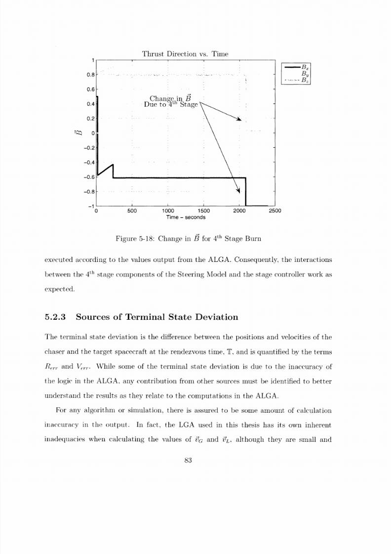
8/13/2019 Lambert Guidance
http://slidepdf.com/reader/full/lambert-guidance 83/122

8/13/2019 Lambert Guidance
http://slidepdf.com/reader/full/lambert-guidance 84/122

8/13/2019 Lambert Guidance
http://slidepdf.com/reader/full/lambert-guidance 85/122
range of coast times used in this thesis are on the order of 10 m and less than 0.1 m/sec,
respectively.
4 th Stage Ignition Timing
Along with the velocity-to-be-gained, the ALGA outputs the burn time, and thrust di-
rection vector of the 4 th stage manoeuver. This burn time, ¶7b, is used by the cut-off
controller to calculate the ignition time of the 4 th stage engine, which is passed to the
stage controller by way of the cut-off signals and is used to tell the engine when to start
burning fel.
As stated in Section 5.1.4, the maximum rate at which the simulation is called is 1000
[Hz.herefore, the minimum lapse in time between when the cut-off signals are updated
and when these updated signals are read by the stage controller is 0.001 seconds. Assuming
that the burn time is calculated to more than three decimal places of accuracy, there is
an associated velocity discrepancy of at most 0.0009 m/sec by the time the 4 th stage burn
is executed. This may seem like a trivial amount of time, but with speeds ranging from 3
to 7 k:m/sec, this discrepancy translates in to a deviation of approximately 3 to 7 meters
f:)r terminal position alone.
4 th"Stage Mass Difference
Dluring the first three boost phases, the Vehicle Staging Model does not know how much
fiuel s going to be expended for the short 4 th stage correction burn as described in Section
5.1.4. Therefore, the 4 th stage mass (M4 th) given by the Vehicle Staging Model does
not account for the reduced mass due to the fuel burn. The calculation of rlb and B 4 th
in the ALGA along with the state propagation by the Runge-Kutta integrator depend
on ilth, which is given as 1100 kg until a more accurate value is calculated. A more
accurate calculation of MAth isn't achieved until the end of the boost phase when the
4 th stage correction burn is executed. Consequently, the values of Ilb and B 4th have a
85

8/13/2019 Lambert Guidance
http://slidepdf.com/reader/full/lambert-guidance 86/122
computational inaccuracy proportional to the mass of the fuel expelled during the 4 th
stage correction burn, which is approximately 1 to 2 kg. This mass difference is small
compared to the total mass of the 4 th stage, but this difference in mass still effects the
terminal state deviation of the chaser.
86
8/13/2019 Lambert Guidance
http://slidepdf.com/reader/full/lambert-guidance 87/122
Chapter 6
ALGA Performance Analysis
After the developn-mentof the Augmented Lambert Guidance Algorithm, as described
in Chapter 4, the task of creating a computer simulation to evaluate the robustness,
versatility, and overall ability of the ALGA was undertaken. Chapter 5 illustrated the
models created to mimic the physical characteristics of the chaser, target spacecraft, and
the environment in which they both operate. These models were then implemented over
time through the use of simulation software. Once the models and the simulation were
completed, the evaluation of the ALGA was able to commence.
The evaluation consists of quantifying how well the ALGA completes the task of
getting the chaser to rendezvous with a target spacecraft in orbit around the Earth. To
this end, a multitude of test cases were created to survey the expected operational region
of the rendezvous missions. But first, the boundaries of this region must be defined. The
boundaries are characterized by several parameters, including the range of mission times,
the likely target orbits, and the possible approach paths that the chaser may take to getto the target spacecraft. Once the range of parameters have been found, the test cases
are created.
After each of these test cases is run, the positions and velocities of both the chaser
and target spacecraft are found at the rendezvous time to calculate Re,, and Ve,,. The
87
8/13/2019 Lambert Guidance
http://slidepdf.com/reader/full/lambert-guidance 88/122
performance of the ALGA is then measured with respect to the success criteria outlined in
Chapter 3. The results of running these various test cases are then plotted and discussed.
6.1 Operational Region
The definition of the operational region is primarily based on the discussion of the possible
types of missions that would use the ALGA, as described in Section 1.1. Conforming to
these mission descriptions, the mission timing and the characterization of the target orbits
are the two major contributors to the boundaries of the operational region.
Because the 4th
stage engine has a finite amount of fuel, it is the most influential factorin determining whether the chaser can rendezvous with the target spacecraft. No matter
how accurate the ALGA computes the values of B 4 th, 7'b, and irTmd, if the chaser does
not have enough fuel to burn for the entire predicted burn time, the chaser will never
rendezvous with the target spacecraft.
Because the success of the rendezvous mission relies heavily on the amount of Ait, any
factor that may increase the required amount of Ai/ must be examined. Therefore, the
two possible approach paths that the chaser is able to take to reach the target will also
be discussed in this section.
6.1.1 Mission Timing
Recall from Section 1.1 that the expected missions employing this algorithm have the
desire to reach the target expeditiously; therefore, the segment of the mission time from
launch to rendezvous, 7, is chosen to be less than an hour.
Furthermore, the LGA used in this thesis has an inherent limitation that restricts the
value of 7. The LGA yields inaccurate results when the coast phase time, Tcp, of the
transfer trajectory is less than 200 seconds. With this constraint and considering that the
possible maximum time for the boost phase, rlBPma is 244 seconds, the lower bound for
88

8/13/2019 Lambert Guidance
http://slidepdf.com/reader/full/lambert-guidance 89/122

8/13/2019 Lambert Guidance
http://slidepdf.com/reader/full/lambert-guidance 90/122
above the Earth at closest approach) greater than 100km. To reduce the number of test
cases, and the ensuing number of results plots, only circular orbits were used during the
evaluation of the ALGA.
Now that the target orbits have been limited to circular trajectories, the next step is
to investigate the possibility of another orbital element effecting the ability of the chaser
to rendezvous with the target spacecraft. There is a property of the target orbit that
has a significant effect on the amount of fuel required by the chaser to rendezvous with
the target spacecraft. This property is the difference in inclination of the target orbit
with respect to the inclination of the chaser's transfer trajectory. As the difference in
inclination between the two spacecraft grows, the required amount of Ai¥ grows as well.
The primary evaluation will focus on the test cases where the chaser is launched in
such a way that it does not have to make a plane change to rendezvous with the target.
By eliminating the plane change, the evaluation of the ALGA will show the maximum
range of successful test cases. Section 6.2.2 illustrates the difference between test cases
that differ by just the inclination change.
6.1.3 Approach Paths
To achieve the rendezvous point from the launch position, there are two possible approach
paths: Overtaking and Head-On. The importance in differentiating the two approach
paths is derived from the amount of Ai¥ that the 4 th stage engine must provide to the
chaser. The velocity characteristics of the two approach paths are briefly discussed here.
Overtaking Trajectory
The Overtaking trajectory is shown in Figure 6-2. For the Overtaking trajectory, the
chaser and target spacecraft are traveling in the same direction before the 4 th stage ma-
noeuver.
In this case, the target spacecraft has a higher speed than the chaser before the 4 th
90

8/13/2019 Lambert Guidance
http://slidepdf.com/reader/full/lambert-guidance 91/122
Chaser Overtaking Target
-0.5 0
X - Earth Radii
0.5 1
Figure 6-2: Overtaking Trajectory
Velocity Comparison
0 500 1000 1500 2000 2500 3000
Time - seconds
Position Comparison
0 500 1000 1500 2000 2500 3000
Time - seconds
Figure 6-3: Overtaking Trajectory - Position and Velocity Comparison
91
1
0.8
0.6
0.4
I 0.2c
w 0
N -0.2
-0.4
-0.6
-0.8
-1
Transfer Trajectto Launch
' .4 ----":t--------- '--------- i
Rendezvous... ' :Point - - -...-
, , - i-1
x 10-3
1
0.5
0
-0.5
-1
0
a,.)
uJ
-cr
C.I
-r-CZ
LU
1
0.5
0
-0.5
-1 . ,'-I
_
r- T . . . .... i ... ;. T I I Ia·
4 ·-ri -·
.·fr
\i
I
-0011
-·,0r . . ..

8/13/2019 Lambert Guidance
http://slidepdf.com/reader/full/lambert-guidance 92/122
stage. Therefore, the chore of the chaser's 4 th stage engine is to provide enough thrust to
increase its speed. Figure 6-3 shows the x, y, and z components of both the velocity and
position for the target spacecraft versus the chaser.
The top graph compares the velocity of the two spacecraft. For this particular set of
initial conditions, the chaser ignites its 4 h stage engine at approximately 2800 seconds.
At this time the chaser's approximate speed is roughly 7.67 km/sec while the target's
is 7.84 km/sec. Additionally, the relative speed between the two spacecraft, since they
are traveling in nearly the same direction, is estimated by simply finding the magnitude
difference between the chaser and target spacecraft. Beginning with a relative velocity
difference of 0.17 km/sec, the chaser executes the 4 th stage burn and both the chaser and
target are traveling at the 7.84 km/sec.
Head-On Trajectory
Figure 6-4 shows the Head-On trajectory. In this situation, the chaser and target space-
craft are traveling in opposite directions toward the same rendezvous point.
Again, the target spacecraft has a higher speed than the chaser before the 4 th stage
manoeuver and needs the thrust from the 4 th stage burn to match the velocity of the
target. However, because the two spacecraft are traveling in opposite directions, the
relative velocity difference between the two cannot be computed by simply finding the
magnitude difference between the two quantities.
The velocity and position comparisons for a Head-On trajectory is shown in Figure 6-
5. The particular Head-On trajectory shown in these graphs requires that the chaser's 4 th
stage engine ignites at roughly 1100seconds, when the chaser's speed is approximately 2.19
km/sec. Meanwhile, the target spacecraft is traveling in roughly the opposite direction at
7.61 km/sec. Because of the approach path, the relative speed between the two craft is
estimated by adding their two respective speeds. Therefore, the relative velocity difference
is roughly 9.8 km/sec.
92

8/13/2019 Lambert Guidance
http://slidepdf.com/reader/full/lambert-guidance 93/122
Chaser Head-On to Target
Transfer Trajectory SpacecraftOrbit
,, . t --- -
: ;-_- _ -- - -i/ 7
. t i
i i "t-~;·; _T; /~T-=-~~-
-1 -0.5 0
X - Earth Radii
0.5
Figure 6-4: Head-On Trajectory
Velocity Comparison
0 200 400 600 800 1000 1200 1400
Time - seconds
Position Comparison
200 400 600 800
Time - seconds
1000 1200 1400
Figure 6-5: Head-On Trajectory - Position and Velocity Comparison
93
0.5
acc
zuJ
N
0
-0.5
-1
x 10- 3
1
0.5
0
-0.5
-1
0a,
cow
a,
c
LU
I
O
.cL
0.5
U
0
- - Zs/crs/cb
rRy- Rz
__/1L
r
·
s r
r . , .. .. e .· . T :' - ' G _ _.
-
1
1
I--
- I- ,A4,- , -
'?T`" '
1
.-
I __ i -

8/13/2019 Lambert Guidance
http://slidepdf.com/reader/full/lambert-guidance 94/122
It can be seen that for this particular set of initial conditions, the 4th stage engine
simply doesn't have enough fuel and thrust capability to match the position and velocity
of the target spacecraft. Recall that the 4th stage engine was designed to provide a
maximum velocity change of 5000 m/sec and that the orbital speed of a spacecraft in
a 100 or 500 km orbit is 7844 or 7612 m/sec, respectively; therefore, for any head-on
trajectory, the chaser's 4th stage engine would have to provide well over 5000 m/sec
of velocity change to rendezvous with the orbiting target spacecraft. So, for the 4th
stage engine and operational regions defined previously, none of the head-on approach
trajectories will result in a successful rendezvous. To verify this, the head-on trajectories
will still be run through the simulation.
Consequently, the evaluation will be performed for both the Overtaking approach
and the Head-On approach over the entire operational region. By looking at trajectories
following both approach paths, the evaluation will better quantify the ability of this
specific 4th stage engine while using the ALGA.
6.1.4 Distances
Previously, Section 2.1.1 discussed the possibility of two solution trajectories between the
launch point and rendezvous point. Because the direction of travel was chosen to only
traverse the "short" route, the transfer angle, , does not exceed 1800. Therefore, the
linear distance (d) measured from the launch point to the rendezvous point, for any given
set of initial conditions, should not exceed a value of twice the radius of the Earth plus
the altitude of the target spacecraft (2r + hl/c). However, when the value of 0 gets in the
vicinity of 180°, the LGA may not be able to distinguish which direction is the "short"
way. Therefore, the actual value of d may be slightly greater than 2ro .
d = rT- R < (2rq3+1 ) (6.2)
94
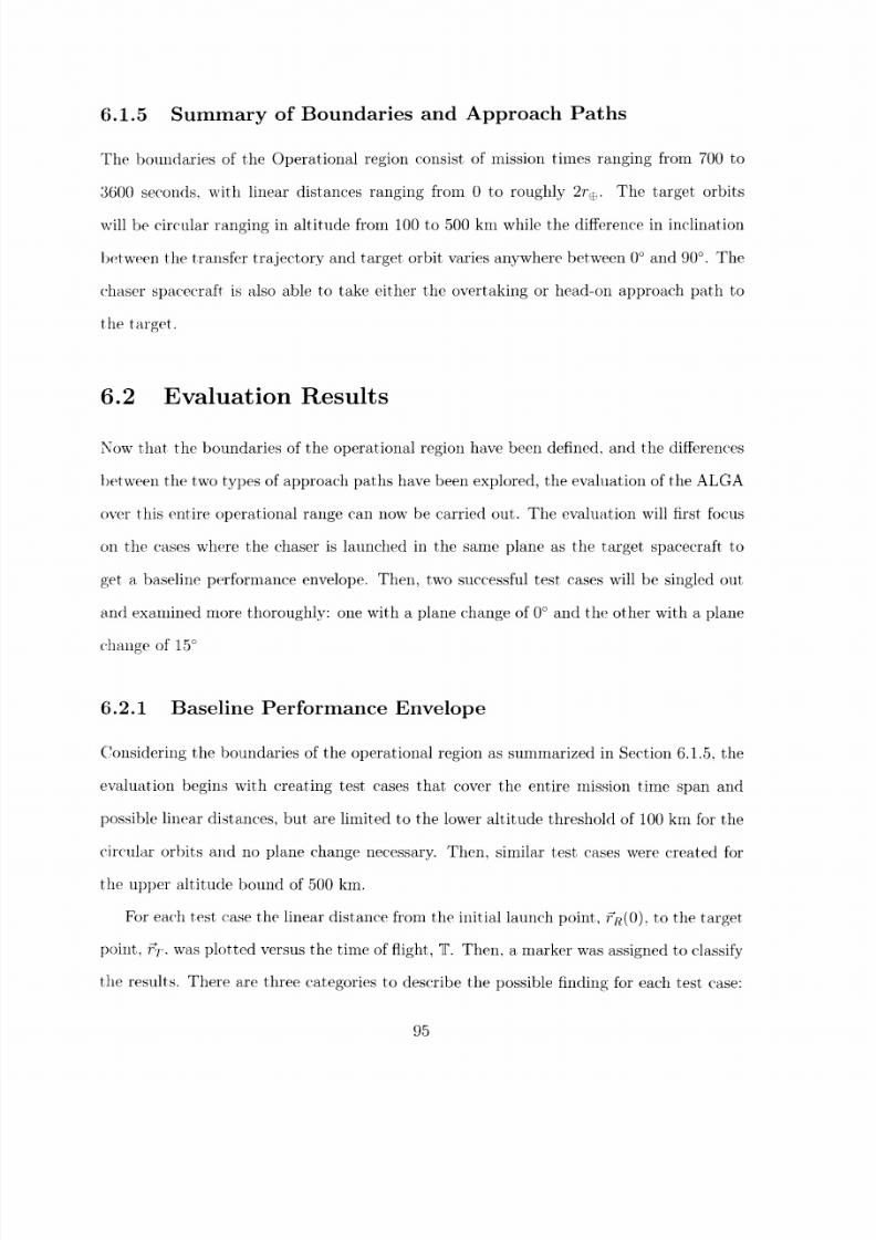
8/13/2019 Lambert Guidance
http://slidepdf.com/reader/full/lambert-guidance 95/122
6.1.5 Summary of Boundaries and Approach Paths
The boundaries of the Operational region consist of mission times ranging from 700 to
3;00 seconds, with linear distances ranging from 0 to roughly 2re. The target orbits
will be circular ranging in altitude from 100 to 500 km while the difference in inclination
between the transfer trajectory and target orbit varies anywhere between 0° and 90°. The
chaser spacecraft is also able to take either the overtaking or head-on approach path to
the target.
6.2 Evaluation Results
Now that the boundaries of the operational region have been defined, and the differences
between the two types of approach paths have been explored, the evaluation of the ALGA
over this entire operational range can now be carried out. The evaluation will first focus
on the cases where the chaser is launched in the same plane as the target spacecraft to
get a baseline performance envelope. Then, two successful test cases will be singled out
and examined more thoroughly: one with a plane change of 0° and the other with a plane
change of 15°
6i.2.1 Baseline Performance Envelope
Considering the boundaries of the operational region as summarized in Section 6.1.5. the
evaluation begins with creating test cases that cover the entire mission time span and
possible linear distances, but are limited to the lower altitude threshold of 100 km for the
circular orbits and no plane change necessary. Then, similar test cases were created for
the upper altitude b)ound of 500 km.
For each test case the linear distance from the initial launch point, R(O),to the target
point, Ft, was plotted versus the time of flight, 'T. Then, a marker was assigned to classify
the results. There are three categories to describe the possible finding for each test case:
95

8/13/2019 Lambert Guidance
http://slidepdf.com/reader/full/lambert-guidance 96/122

8/13/2019 Lambert Guidance
http://slidepdf.com/reader/full/lambert-guidance 97/122
TOF vs Distance - 100 km Height - Overtake~~~~~~~,. . .,
1000 1500 2000 2500 3000 3500Time (seconds)
* Good
x Not Enough Fuel
O Runs Into Earth
Figure 6-6: ¶ vs. Distance - 100km - Overtaking Target
TOF vs Distance - 100 km Height - Head On
O x xo ° . ,'0O 0 0 0o0 0 00 0 0 0 .
O0 0 0 0 0 0
0 00 0
0000 0
0
I 1 ~i·F i
500 1000 1500 2000 2500 3000 3500Time (seconds)
Not Enough FuelO Runs Into Earth
Figure 6-7: vs. Distance - 100km- Heading to Target
97
2
1.5
0r
LU
1-
. _
0.5
0-00 -0- 0 k0 i O00 ;T· s. o oooo o ...000 0 0 0
O 0 ** * O ~ *~*
0 O -
,-*
*,
O O * ,0 * .
.* . .
X X
I IK X :,(
x x x
x x, x x i x xx x~~~~~~~~~~~~~~~~~~~~~~
500
2
: 1.50CZ
t:
-
U)
0q)
0.5
-
IV,
11
"I
I
t
x
I
XI11 _ I
I !

8/13/2019 Lambert Guidance
http://slidepdf.com/reader/full/lambert-guidance 98/122
TOF vs Distance - 500 km Height - Overtake, .... ~~~~~~~~~~~~~~~~~~~~~~~~~~~~~~~~~~~~~~~~~~~~~~~~~~~
000oo 0000- oO Il.. oC) O U
0
0 0 o
0-
0O
0
0
00 o
0 *0 *
0 a0 , *
0 * * *
* X
x.~' x,
0 0
, o0 0o **
* * A,, o
a
X
x
x x
A
0o000
x.
Xx
X
x'
... : X. .
xx
x
X a X
ooO 8tQ, ti, .t f'00 0' :...
* *** * ** *
x* * ** * *
a
x
X ;. x ...
A
x-x( x
* x ·x' '
%: x ~~xA A
'A'A
0.5
05(
00 1000 1500 2000 2500 3000 3500
Time (seconds)
* Good
x Not Enough Fuel
O Runs Into Earth
Figure 6-8: vs. Distance - 500km - Overtaking Target
TOF vs Distance - 500 km Height - Head On
O o x.°o °0o 00 000 .0 x0 0 0 x x ' xx x x0A x
0 0 X
0 0A '
0 0
)O 1000 1500 2000 2500 3000 3500
Time (seconds)
x Not Enough Fuel
O Runs Into Earth
Figure 6-9: ¶ vs. Distance - 500km - Heading to Target
98
2
1.5.E5
c
c:C.
U
1
0.5
05(
2
1.5:5CZ
It
(U"oU)CCZLU)0"'
a~
o O
1

8/13/2019 Lambert Guidance
http://slidepdf.com/reader/full/lambert-guidance 99/122

8/13/2019 Lambert Guidance
http://slidepdf.com/reader/full/lambert-guidance 100/122

8/13/2019 Lambert Guidance
http://slidepdf.com/reader/full/lambert-guidance 101/122

8/13/2019 Lambert Guidance
http://slidepdf.com/reader/full/lambert-guidance 102/122

8/13/2019 Lambert Guidance
http://slidepdf.com/reader/full/lambert-guidance 103/122
8/13/2019 Lambert Guidance
http://slidepdf.com/reader/full/lambert-guidance 104/122
8/13/2019 Lambert Guidance
http://slidepdf.com/reader/full/lambert-guidance 105/122
Tb & B34th
Figures 6-14 to 6-15 both show a similar trend in the calculation of Tb, and B 4 th: the
values start with the Initialization block value and exponentially reach their final value
over the course of the boost phase. The final values of 'Tb, and Bth are then used to
execute the 4 th stage manoeuver. Per the discussion of zone predictability in Section
6.2.1, the value of Av is expected to change over the course of the boost phase. This is
confirmed by Figure 6-14 showing approximately 315 m/sec and 265 m/sec decrease in
t;he predicted Av versus the ending Av for the 0° plane change and 15° plane change,
respectively. These figures also show that the amount of Av is substantially greater for
the 150plane change trajectory than the 0° plane change trajectory, which was expected.
With the decreasing value of Av as time progresses, the value of the burn time de-
creases accordingly, due to the dependance of the burn time on the required amount of
Au. Hence, the burn time is greater for the 150plane change trajectory than the 0 plane
change trajectory.
iAccuracy
With the values of iT,,od, Tb, and B 4th calculated for these two trajectories, the next logical
step is to look at the accuracy as measured by the quantities R,,rr and V,.,. described in
Section 3.4. The values of Rerr and Verr llustrate how well the ALGA was able to guide
the chaser during boost, calculate the proper ignition time, and determine thrust direction
of the 4 th stage manoeuver, which drives the chaser to match the position and velocity of
the target spacecraft.
Before looking at the exact values of Rer and Ve,, the position and velocity of both
the 0 plane change test case and 15° plane change test case are compared to the position
and velocity of the target spacecraft. Figures 6-16 and 6-17 show the comparisons for
each of the test cases. These figures confirm that the position of the chaser in both test
cases reaches the vicinity of the target spacecraft with comparable velocities.
105

8/13/2019 Lambert Guidance
http://slidepdf.com/reader/full/lambert-guidance 106/122
Av vs. Time
Time - seconds
Figure 6-14: Av vs. Time for 0° and 15° Plane Change
r- Odeg I
15deg
Tb vs. Time
50 100 150 200 250
Time - seconds
I--- Odeg
15deg
300
Figure 6-15: Tb vs. Time for 0° and 15° Plane Change
106
rd7:0C-)C)
$Cl
C),I<L
.1
240
235
230
vD //O
C)c 220
[ 215
210
205
9nn0

8/13/2019 Lambert Guidance
http://slidepdf.com/reader/full/lambert-guidance 107/122
Velocity Comparison
1000 1500
Time - seconds
Position Comparison
1000 1500
Time - seconds
2000 25
2000
--s/cx
... s/cz
I-VRzRy... , Rz
00
- r-/crs/c,
rRx
rRy.... Rz
2500
Figure 6-16: and i Comparison for 0 Plane Change
Velocity Comparison
1000 1500
Time - seconds
Position Comparison
1000 1500
Time - seconds
2000
2000
2500
- - s/cars/cb
rRxrRyTRz
500
Figure 6-17: Fiand i Comparison for 00 Plane Change
107
Vo0a,cn
in
a)
EI
.)oa)
5000
0
-5000
''·~~~~Nb -~~~~
0 500
x 106
Ea,CD)a,EIc
oC)
0.0_oa-
5
0
-5
0r
44- ~ ~~~~
I%%I
iIi i i~N
0 500
C:00a)
a,EI
0
5000
0
-5000
0 500
I - - -
x 106
._a,E
C
5
0
-5
- -
Nb
NbNb
NbNb
Nb
0 500 2

8/13/2019 Lambert Guidance
http://slidepdf.com/reader/full/lambert-guidance 108/122

8/13/2019 Lambert Guidance
http://slidepdf.com/reader/full/lambert-guidance 109/122

8/13/2019 Lambert Guidance
http://slidepdf.com/reader/full/lambert-guidance 110/122
8/13/2019 Lambert Guidance
http://slidepdf.com/reader/full/lambert-guidance 111/122

8/13/2019 Lambert Guidance
http://slidepdf.com/reader/full/lambert-guidance 112/122

8/13/2019 Lambert Guidance
http://slidepdf.com/reader/full/lambert-guidance 113/122

8/13/2019 Lambert Guidance
http://slidepdf.com/reader/full/lambert-guidance 114/122

8/13/2019 Lambert Guidance
http://slidepdf.com/reader/full/lambert-guidance 115/122

8/13/2019 Lambert Guidance
http://slidepdf.com/reader/full/lambert-guidance 116/122

8/13/2019 Lambert Guidance
http://slidepdf.com/reader/full/lambert-guidance 117/122
fl.
I/
/
{/
LI,
Figure A-2: Hyperbolic Transfer
=C- /(A. 15)a
aF = 1--(1 - cosh2) (A.16)
I
G= I- j (sinh 21- 2) (A. 17)
F =- J/ sinh (A.18)r 12
aG = 1----(1 -cosh 2) (A.19)
'r2
117

8/13/2019 Lambert Guidance
http://slidepdf.com/reader/full/lambert-guidance 118/122

8/13/2019 Lambert Guidance
http://slidepdf.com/reader/full/lambert-guidance 119/122

8/13/2019 Lambert Guidance
http://slidepdf.com/reader/full/lambert-guidance 120/122
[This page intentionally left blank.]

8/13/2019 Lambert Guidance
http://slidepdf.com/reader/full/lambert-guidance 121/122

8/13/2019 Lambert Guidance
http://slidepdf.com/reader/full/lambert-guidance 122/122