lanczos algorithm: theory and...
TRANSCRIPT
m
Preliminaries
Krylov subspaces
Iteration scheme
Application: S=1 BAHC
Application: S=1/2 XYchain
Application: S=1/2 Ising intransversal field (ITF)
Lanczos Algorithm: Theory and Aplications
J. Almeida1,2
1Department of Theoretical Physics, University of Ulm (Ulm, Germany)2 these notes are largely based on the book "Matrix Computations", by G. H. Gollub and C. F. Van
Loan
York (United Kingdom), April 2012

m
Preliminaries
Krylov subspaces
Iteration scheme
Application: S=1 BAHC
Application: S=1/2 XYchain
Application: S=1/2 Ising intransversal field (ITF)
Outline
1 Preliminaries
2 Krylov subspaces
3 Iteration scheme
4 Application: S=1 Bond-alternating Heisenberg chain
5 Application: S=1/2 XY-Heisenberg chain
6 Application: S=1/2 ITF

m
Preliminaries
Krylov subspaces
Iteration scheme
Application: S=1 BAHC
Application: S=1/2 XYchain
Application: S=1/2 Ising intransversal field (ITF)
Eigensystem solution in many-body systems
Problem: Huge Hilbert spaces in many-body systems
Sztotal S = 3
2 S = 1 S = 12
0 1.703.636 73.789 9241 1.650.792 69.576 7922 1.501.566 58.278 4953 1.281.280 43.252 2204 1.024.464 28.314 665 766.272 16.236 126 534.964 8.074 17 347.568 3.4328 209.352 1.2219 116.336 352
10 59.268 7811 27.456 1212 11.440 113 4.22414 1.35315 36416 7817 1218 1
Table: Dimension of sectors with well defined total z-axis spin projection in aL = 12 spin chain. Note: an 8-byte representation of a 11585× 11585 matrixoccupies 1GB of memory.

m
Preliminaries
Krylov subspaces
Iteration scheme
Application: S=1 BAHC
Application: S=1/2 XYchain
Application: S=1/2 Ising intransversal field (ITF)
Lanczos algorithm: Preliminaries
Theorem (Courant-Fischer Minimax Theorem):
If A ∈ Rn×n is symmetric then, for k = 1 . . . n:
λk(A) = maxdim(S)=k
min0 6=y∈S
yT AyyT y
(1)
with λn(A) ≤ λn−1(A) ≤ · · · ≤ λ2(A) ≤ λ1(A) the egenvalues of A.
Extremal Eigenvalues:
i/ k = 1:
λ1(A) = maxyT AyyT y
(2)
ii/ k = n:
λn(A) = minyT AyyT y
(3)
m
Preliminaries
Krylov subspaces
Iteration scheme
Application: S=1 BAHC
Application: S=1/2 XYchain
Application: S=1/2 Ising intransversal field (ITF)
Lanczos algorithm: Preliminaries
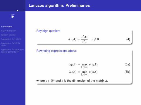
Rayleigh quotient
r(x;A) =xT AxxT x
x 6= 0 (4)
Rewritting expressions above
λ1(A) = max‖y‖=1
r(y;A) (5a)
λn(A) = min‖y‖=1
r(y;A) (5b)
where y ∈ Rn and n is the dimension of the matrix A.
m
Preliminaries
Krylov subspaces
Iteration scheme
Application: S=1 BAHC
Application: S=1/2 XYchain
Application: S=1/2 Ising intransversal field (ITF)
Lanczos algorithm: preliminaries
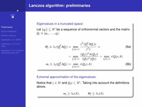
Eigenvalues in a truncated space:
Let {qi} ⊆ Rn be a sequence of orthonormal vectors and the matrixQj ≡ [q1, . . . , qj].
Mj ≡ λ1(QTj AQj) = max
‖y‖=1
yT(QTj AQj)y
yT y= (6a)
= max‖y‖=1
(Qjy)T A(Qjy)(Qy)T(Qy)
= max‖y‖=1
r(Qjy;A)
mj ≡ λj(QTj AQj) = min
‖y‖=1r(Qjy;A) (6b)
Extremal approximation of the eigenvalues:
Notice that y ∈ Rj and Qjy ⊂ Rn. Taking into account the definitionsabove,
mj ≥ λn(A), Mj ≤ λ1(A).

m
Preliminaries
Krylov subspaces
Iteration scheme
Application: S=1 BAHC
Application: S=1/2 XYchain
Application: S=1/2 Ising intransversal field (ITF)
Lanczos algorithm: preliminaries
Eigenvalues in a truncated space:
Let {qi} ⊆ Rn be a sequence of orthonormal vectors and the matrixQj ≡ [q1, . . . , qj].
Mj ≡ λ1(QTj AQj) = max
‖y‖=1
yT(QTj AQj)y
yT y= (7a)
= max‖y‖=1
(Qjy)T A(Qjy)(Qy)T(Qy)
= max‖y‖=1
r(Qjy;A)
mj ≡ λj(QTj AQj) = min
‖y‖=1r(Qjy;A) (7b)
Extremal approximation of the eigenvalues:
The lanczos algorithm can be derived by considering how togenerate the qj vectors so that mj and Mj are increasingly betterestimates of λn(A) and λ1(A).
m
Preliminaries
Krylov subspaces
Iteration scheme
Application: S=1 BAHC
Application: S=1/2 XYchain
Application: S=1/2 Ising intransversal field (ITF)
Lanczos algorithm: Krylov subspaces
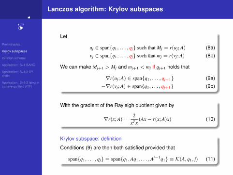
Let
uj ∈ span{q1, . . . , qj} such that Mj = r(uj;A) (8a)
vj ∈ span{q1, . . . , qj} such that mj = r(vj;A) (8b)
We can make Mj+1 > Mj and mj+1 < mj if qj+1 holds that
∇r(uj;A) ∈ span{q1, . . . , qj+1} (9a)
−∇r(vj;A) ∈ span{q1, . . . , qj+1} (9b)
With the gradient of the Rayleigh quotient given by
∇r(x;A) =2
xT x(Ax− r(x;A)x) (10)
Krylov subspace: definition
Conditions (9) are then both satisfied provided that
span{q1, . . . , qj} = span{q1,Aq1, . . . ,Aj−1q1} ≡ K(A, q1, j) (11)
m
Preliminaries
Krylov subspaces
Iteration scheme
Application: S=1 BAHC
Application: S=1/2 XYchain
Application: S=1/2 Ising intransversal field (ITF)
Lanczos algorithm: Krylov subspaces
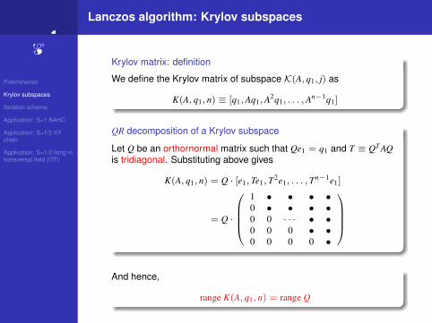
Krylov matrix: definition
We define the Krylov matrix of subspace K(A, q1, j) as
K(A, q1, n) ≡ [q1,Aq1,A2q1, . . . ,An−1q1]
QR decomposition of a Krylov subspace
Let Q be an orthornormal matrix such that Qe1 = q1 and T ≡ QT AQis tridiagonal. Substituting above gives
K(A, q1, n) = Q · [e1, Te1, T2e1, . . . , Tn−1e1]
= Q ·
1 • • • •0 • • • •0 0 · · · • •0 0 0 • •0 0 0 0 •
And hence,
range K(A, q1, n) = range Q
m
Preliminaries
Krylov subspaces
Iteration scheme
Application: S=1 BAHC
Application: S=1/2 XYchain
Application: S=1/2 Ising intransversal field (ITF)
Lanczos algorithm: recapitulation of main ideas
First idea
We have seen that the maximal eigevalues of a certainsymmetric matrix A restricted to the Krylov subspace K(A, q1, j) givebetter estimates upon increasing the dimension j (since it ’follows’the gradient of the Rayleigh quotient)
In general, the operations of truncation and diagonalisation of thematrix A in this new space are numerically costly.
Second idea
We have seen however that in principle it is possible to find anorthonormal basis of the Krylov space K(A, q1, j) such that thematrix A restricted to this space and written in this basis has atridiagonal form: this shots with the same stone the costs ofobtaining iteratively better estimates of the original eigensystem.

m
Preliminaries
Krylov subspaces
Iteration scheme
Application: S=1 BAHC
Application: S=1/2 XYchain
Application: S=1/2 Ising intransversal field (ITF)
Lanczos algorithm: iteration equations
By definition
T = QT AQ ≡
α1 β1 · · · 0
β1 α2. . .
.... . .
. . .. . .
.... . .
. . . βj−10 · · · βj−1 αn
with
{αi = qT
i Aqi
βi = qTi+1Aqi
By construction
QA = TQ⇐⇒ [Aq1, Aq2, . . . , Aqn] =
= [α1q1 + β1q2, β1q1 + α2q2 + β2q3, . . . , βn−1qn−1 + αnqn]
q2 = 1/β1(A− α1)q1
q3 = 1/β2{(A− α2)q2 − β1q1
}· · ·qk = 1/βk−1
{(A− αk−2)qk−1 − βk−2qk−2
}, 2 < k < n
0 = (A− αn)qn − βn−1qn−1
m
Preliminaries
Krylov subspaces
Iteration scheme
Application: S=1 BAHC
Application: S=1/2 XYchain
Application: S=1/2 Ising intransversal field (ITF)
Lanczos algorithm: iteration equations
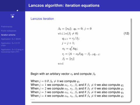
Lanczos iteration
β0 = ‖r0‖; q0 = 0; j = 0
while(βj 6= 0) (12)
qj+1 = rj/βj;
j = j + 1;
αj = qTj Aqj;
rj = (A− αjI)qj − βj−1qj−1;
βj = ‖rj‖end
Begin with an arbitary vector r0 and compute β0
When j = 0 if β0 6= 0 we compute q1When j = 1 we compute α1, r1, β1 and if β1 6= 0 we also compute q2When j = 2 we compute α2, r2, β2 and if β2 6= 0 we also compute q3When j = 3 we compute α3, r3, β3 and if β3 6= 0 we also compute q4When j = 4 we compute α4, r4, β4 and if β4 6= 0 we also compute q5· · ·

m
Preliminaries
Krylov subspaces
Iteration scheme
Application: S=1 BAHC
Application: S=1/2 XYchain
Application: S=1/2 Ising intransversal field (ITF)
Lanczos algorithm: a simplest example
Matlab(R) code% Create a random symmetric matrixD=200for i=1:D,for j=1:i,A(i,j)=rand;A(j,i)=A(i,j);
endend
% Iteration with j=0r0=rand(D,1);b0=sqrt(r0’*r0);q1=r0/b0;a1=q1’*A*q1
% Iteration with j=1r1=A*q1-a1*q1;b1=sqrt(r1’*r1)q2=r1/b1;a2=q2’*A*q2
% Iteration with j=2r2=A*q2-a2*q2-b1*q1;b2=sqrt(r2’*r2)q3=r2/b2;a3=q3’*A*q3
% Create matrix QQ=[q1 q2 q3];% Check orthogonalityEYE=Q’*Q% Check the tridiagonal truncationT=Q’*A*Q
Outputoctave:6> lanczosD = 200a1 = 3.6694b1 = 1.2412a2 = 0.18896b2 = 0.82261a3 = -0.38889EYE =
1.0000 0.0 0.00.0 1.0000 0.00.0 0.0 1.0000
T =
3.6694 1.2412 0.01.2412 0.1889 0.8226
0.0 0.8226 -0.3888

m
Preliminaries
Krylov subspaces
Iteration scheme
Application: S=1 BAHC
Application: S=1/2 XYchain
Application: S=1/2 Ising intransversal field (ITF)
Lanczos algorithm: othogonality and termination of theiteration
Theorem: othogonality and termination
Theorem: Let A ∈ Rn×n be symmetric and assume q1 ∈ Rn has unit2-norm. Then the Lanczos iteration (12) runs until j = m wherem = rank K(A, q1, n).
Moreover, for j = 1 : m we have that Qj = [q1, . . . , qj] hasorthonormal columns that span K(A, q1, j).
Corollary: βj = 0⇐⇒ span K(A, q1, j + 1) ⊆ span K(A, q1, j)

m
Preliminaries
Krylov subspaces
Iteration scheme
Application: S=1 BAHC
Application: S=1/2 XYchain
Application: S=1/2 Ising intransversal field (ITF)
Lanczos algorithm: headers of a complete Lanczos routine
Restart mode routine
void findEigenvectors_restartMode(int nev, int ncv, int& nit, double tol,const base_Obj& seed,vector<double>& evalue,vector<base_Obj*>& evector,double& min_beta, double& err,double zero_modes_shift=0.0 )
Low-level restart mode routine
void findEigenvectors(int nev, int ncv, int& nit, double tol,const base_Obj& seed,vector<double>& evalue,vector<base_Obj*>& evector,double& min_beta, double& err,int target_nev=-1,vector<double> rm_evalue=vector<double>(0),vector<base_Obj*> rm_evector=vector<base_Obj*>(0),double zero_modes_shift=0.0)

m
Preliminaries
Krylov subspaces
Iteration scheme
Application: S=1 BAHC
Application: S=1/2 XYchain
Application: S=1/2 Ising intransversal field (ITF) Application 1
S=1 Bond-alternated Heisenberg chain:measuring the hidden AKLT order

m
Preliminaries
Krylov subspaces
Iteration scheme
Application: S=1 BAHC
Application: S=1/2 XYchain
Application: S=1/2 Ising intransversal field (ITF)
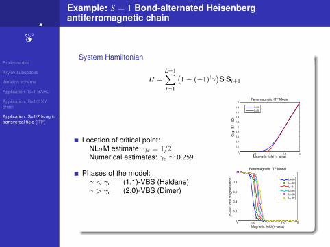
Example: S = 1 Bond-alternated Heisenbergantiferromagnetic chain
System Hamiltonian
H =
L−1∑i=1
(1− (−1)iγ
)SiSi+1
The ground states of this model are particular realizations of the valencebond solids (VBS) as described by Affleck, Kennedy, Lieb and Tasaki(see next slide).
Critical properties and phases
Location of critical point:NLσM estimate: γc = 1/2Numerical estimates: γc ' 0.259
Phases of the model:γ < γc (1,1)-VBS (Haldane)γ > γc (2,0)-VBS (Dimer)

m
Preliminaries
Krylov subspaces
Iteration scheme
Application: S=1 BAHC
Application: S=1/2 XYchain
Application: S=1/2 Ising intransversal field (ITF)
AKLT Physics
AKLT Hamiltonian
HAKLT =
L−1∑i=1
SiSi+1 + β(SiSi+1)2, β = − 1
3
The exact ground state of this model can be expressed using anextended S = 1/2 Hilbert space and is denoted as m = 1, n = 1 valencebond solid (i.e, a (1,1)-VBS).
Properties of the ground state
The AKLT antiferromagnet has continuous SU(2) symmetry,exponentially decaying correlations, a gap and a unique infinitevolume ground state.
with OBC there exist four orthogonal ground states (1 singlet, 1triplet).
with PBC the ground state is unique (1 singlet).
All these ground states converge to the same one in the infinitevolume limit.

m
Preliminaries
Krylov subspaces
Iteration scheme
Application: S=1 BAHC
Application: S=1/2 XYchain
Application: S=1/2 Ising intransversal field (ITF)
AKLT Physics
Hidden order of the ground state
In the usual z-axis projection basis, the AKLT ground state reveals ahidden antiferromagnetic order:
|ψ0〉 = C1| . . . 0+0−0+−+000−. . . 〉+C2| . . . 00+−+00−0+0−. . . 〉+. . .
We say it is topological order because:It is conditioned by the configuration of the degrees of freedom at
the endsIt can not be detected by means of local operators
String Order Parameter
The AKLT order can bedetected with a non local orderparameter mapped from theoryof preroughening surfacetransitions:
Ostr = lim|i−j|→∞
⟨S z
i
j−1∏k=i
eiπS zk S z
j
⟩

m
Preliminaries
Krylov subspaces
Iteration scheme
Application: S=1 BAHC
Application: S=1/2 XYchain
Application: S=1/2 Ising intransversal field (ITF)
Example: exactly solvable XY model
Computing the String Order Parameter
0.0
0.1
0.2
0.3
0.4
0.0 0.1 0.2 0.3 0.4
SO
P
γ
S=1 Bold-Alternating Heisenberg Chain (OBC)
DMRG, L=350
DMRG, L=90
0 0.2 0.4 0.6 0.8 10
0.1
0.2
0.3
0.4
γ
SO
P
S=1 Bond−alternating Heisenberg chain (PBC)
Lanczos, L=14

m
Preliminaries
Krylov subspaces
Iteration scheme
Application: S=1 BAHC
Application: S=1/2 XYchain
Application: S=1/2 Ising intransversal field (ITF) Application 2
S=1/2 Heisenberg XY chain: an integrablesystem

m
Preliminaries
Krylov subspaces
Iteration scheme
Application: S=1 BAHC
Application: S=1/2 XYchain
Application: S=1/2 Ising intransversal field (ITF)
Example: exactly solvable XY model
Hamiltonian (with Periodic Boundary Conditions)
HXY = −12
L−1∑j=1
(σxi σ
xi+1 + σy
i σyi+1)− (σx
1σxL + σy
1σyL)
= −σ+1 σ−L − σ
−1 σ
+L +
L−1∑j=1
{− σ+
i σ−i+1 − σ
−i σ
+i+1
}
with σ±j = 12 (σ
xj ± iσy
j )
Jordan-Wigner transformation
HXY = −L−1∑j=1
(C†i Ci+1 + CiC†i+1)− (−1)NF+1(C†1 CL + C1C†L)
with C±m =
m−1∏j=1
(−σzj )σ±m , and NF the total number of fermions
.

m
Preliminaries
Krylov subspaces
Iteration scheme
Application: S=1 BAHC
Application: S=1/2 XYchain
Application: S=1/2 Ising intransversal field (ITF)
Example: exactly solvable XY model
Fourier-Transforming Hamiltonian
aq =1√
L
L∑m=1
eiqmCm, Cm =1√
L
∑q
e−iqmaq
L−1∑j=1
C†j Cj+1 =1L
L−1∑j=1
∑qq′
a†q aq′e−i(q′−q)je−iq′
L−1∑j=1
C†j+1Cj =1L
L−1∑j=1
∑qq′
a†q aq′ei(q−q′)jeiq
±(C†1 CL + C1C†L) =1L
∑qq′
(a†q aq′eiqLe−iq′ e−iq′L︸ ︷︷ ︸±1
+a†q aq′eiqe−iq′L eiqL︸︷︷︸±1
)
with the choice of momentum boundary conditions:{if NF odd eiqL = +1⇒ q = 2π
L kif NF even eiqL = −1⇒ q = 2π
L k + πL

m
Preliminaries
Krylov subspaces
Iteration scheme
Application: S=1 BAHC
Application: S=1/2 XYchain
Application: S=1/2 Ising intransversal field (ITF)
Example: exactly solvable XY model
Diagonal form of the Hamiltonian
HXY = −1L
∑qq′
a†q aq′
e−iq′( L−1∑
j=1
e−i(q′−q)j + e−i(q′−q)L)
+
+ eiq( L−1∑
j=1
ei(q−q′)j + ei(q−q′)L) = −2
∑q
cos(q)a†q aq
Ground state energy of a XY-spin chain with PBC
The lowest energy configuration corresponds exactly to L/2fermions with momenta in the semicircle with positive cosine.
Since boundary conditions are periodic (in contrast with anti-periodic) we have to consider L even and hence momenta of theform q = 2πk/L + π/L.
The momenta that fulfill at the same time the conditions above canbe parametrized as q̃k = −π/2 + (2k − 1)π/L, with k = 1 . . . L/2
Hence, E0XY = −2
L/2∑k=1
cos(q̃k)a†q aq =−2
sin(π/L)
m
Preliminaries
Krylov subspaces
Iteration scheme
Application: S=1 BAHC
Application: S=1/2 XYchain
Application: S=1/2 Ising intransversal field (ITF)
Example: exactly solvable XY model
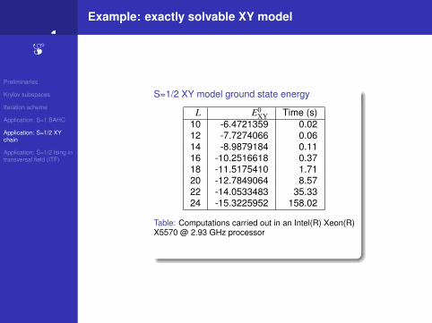
S=1/2 XY model ground state energy
L E0XY Time (s)
10 -6.4721359 0.0212 -7.7274066 0.0614 -8.9879184 0.1116 -10.2516618 0.3718 -11.5175410 1.7120 -12.7849064 8.5722 -14.0533483 35.3324 -15.3225952 158.02
Table: Computations carried out in an Intel(R) Xeon(R)X5570 @ 2.93 GHz processor

m
Preliminaries
Krylov subspaces
Iteration scheme
Application: S=1 BAHC
Application: S=1/2 XYchain
Application: S=1/2 Ising intransversal field (ITF) Application 3
S=1/2 Ising in transversal field: a mostparadigmatic model
m
Preliminaries
Krylov subspaces
Iteration scheme
Application: S=1 BAHC
Application: S=1/2 XYchain
Application: S=1/2 Ising intransversal field (ITF)
Example: S = 1 Bond-alternated Heisenbergantiferromagnetic chain
System Hamiltonian
H =
L−1∑i=1
(1− (−1)iγ
)SiSi+1
Location of critical point:NLσM estimate: γc = 1/2Numerical estimates: γc ' 0.259
Phases of the model:γ < γc (1,1)-VBS (Haldane)γ > γc (2,0)-VBS (Dimer)
0 0.5 1 1.5 20
0.2
0.4
0.6
0.8
1
1.2
1.4
1.6
1.8
2
Magnetic field (x−axis)
Ga
p (
E1
−E
0)
Ferromagnetic ITF Model
L=10
L=20
0 0.5 1 1.5 20
0.2
0.4
0.6
0.8
1
Magnetic field (x−axis)z−
axis
to
tal m
ag
ne
tiza
tio
n
Ferromagnetic ITF Model
L=10
L=12
L=14
L=16
L=18
L=20
m
Preliminaries
Krylov subspaces
Iteration scheme
Application: S=1 BAHC
Application: S=1/2 XYchain
Application: S=1/2 Ising intransversal field (ITF)
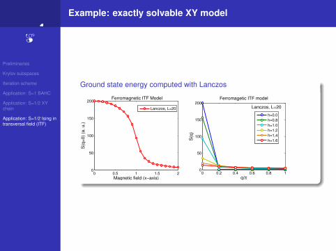
Example: exactly solvable XY model
Ground state energy computed with Lanczos
0 0.5 1 1.5 20
50
100
150
200
Magnetic field (x−axis)
S(q
=0
) (a
. u
.)
Ferromagnetic ITF Model
Lanczos, L=20
0 0.2 0.4 0.6 0.8 10
50
100
150
200Ferromagetic ITF model
q/π
S(q
)
h=0.0
h=0.8
h=1.0
h=1.2
h=1.4
h=1.6
Lanczos, L=20