land inequality and the origin of divergence and

DISCUSSION PAPER SERIES

ABCD

www.cepr.org

Available online at: www.cepr.org/pubs/dps/DP3817.asp www.ssrn.com/xxx/xxx/xxx

No. 3817

LAND INEQUALITY AND THE ORIGIN OF DIVERGENCE AND OVERTAKING IN THE GROWTH

PROCESS: THEORY AND EVIDENCE

Oded Galor, Omer Moav and Dietrich Vollrath

INTERNATIONAL MACROECONOMICS

ISSN 0265-8003

LAND INEQUALITY AND THE ORIGIN OF DIVERGENCE AND OVERTAKING IN THE GROWTH

PROCESS: THEORY AND EVIDENCE

Oded Galor, Brown University and CEPR Omer Moav, Hebrew University of Jerusalem and CEPR

Dietrich Vollrath, Brown University

Discussion Paper No. 3817 March 2003

Centre for Economic Policy Research 90–98 Goswell Rd, London EC1V 7RR, UK

Tel: (44 20) 7878 2900, Fax: (44 20) 7878 2999 Email: [email protected], Website: www.cepr.org

This Discussion Paper is issued under the auspices of the Centre’s research programme in INTERNATIONAL MACROECONOMICS. Any opinions expressed here are those of the author(s) and not those of the Centre for Economic Policy Research. Research disseminated by CEPR may include views on policy, but the Centre itself takes no institutional policy positions.

The Centre for Economic Policy Research was established in 1983 as a private educational charity, to promote independent analysis and public discussion of open economies and the relations among them. It is pluralist and non-partisan, bringing economic research to bear on the analysis of medium- and long-run policy questions. Institutional (core) finance for the Centre has been provided through major grants from the Economic and Social Research Council, under which an ESRC Resource Centre operates within CEPR; the Esmée Fairbairn Charitable Trust; and the Bank of England. These organizations do not give prior review to the Centre’s publications, nor do they necessarily endorse the views expressed therein.

These Discussion Papers often represent preliminary or incomplete work, circulated to encourage discussion and comment. Citation and use of such a paper should take account of its provisional character.

Copyright: Oded Galor, Omer Moav and Dietrich Vollrath

CEPR Discussion Paper No. 3817

March 2003

ABSTRACT

Land Inequality and the Origin of Divergence and Overtaking in the Growth Process: Theory and Evidence*

This research suggests that the distribution of land within and across countries affected the nature of the transition from an agrarian to an industrial economy, generating diverging growth patterns across countries. Land abundance, which was beneficial in early stages of development, generated in later stages a hurdle for human capital accumulation and economic growth among countries in which land ownership was unequally distributed. The qualitative change in the role of land in the process of industrialization affected the transition to modern growth and has brought about changes in the ranking of countries in the world income distribution. Some land abundant countries that were associated with the club of the rich economies in the pre-industrial revolution era and were marked by an unequal distribution of land, were overtaken in the process of industrialization by land scarce countries and were dominated by other land abundant economies in which land distribution was rather equal. The theory focuses on the economic incentives that led landowners to resist growth enhancing educational expenditure. The basic premise of this research, regarding the negative effect of land inequality on public expenditure on education is supported empirically based on cross-state data from the High School Movement in the first half of the 20th century in the US.

JEL Classification: O10 and O40 Keywords: development, growth, human capital accumulation and land inequality

Oded Galor Department of Economics Brown University Providence RI 02912 USA Tel: (1 972) 281 6071 Fax: (1 401) 863 1970 Email: [email protected] For further Discussion Papers by this author see: www.cepr.org/pubs/new-dps/dplist.asp?authorid=110467

Omer Moav Department of Economics Hebrew University of Jerusalem Mt. Scopus Jerusalem 91905 ISRAEL Tel: (972 2) 588 3121 Fax: (972 2) 581 6017 Email: [email protected] For further Discussion Papers by this author see: www.cepr.org/pubs/new-dps/dplist.asp?authorid=143936

Dietrich Vollrath Department of Economics Brown University Providence RI 02912 USA Email: [email protected] For further Discussion Papers by this author see: www.cepr.org/pubs/new-dps/dplist.asp?authorid=158770

*We thank Josh Angrist, Andrew Foster, Eric Gould, Vernon Henderson, Saul Lach, Victor Lavy, Daniele Paserman, and David Weil for helpful discussions and seminar participants at Brown University, Tel-Aviv University, the NBER Summer Institute, 2002, and the Economics of Water and Agriculture, 2002, for helpful comments. Galor’s research is supported by NSF Grant SES-0004304.

Submitted 07 February 2003

1 Introduction

This research suggests that the distribution of land within and across countries affected

the nature of the transition from an agrarian to an industrial economy, generating di-

verging growth patterns across countries. Land abundance, which was beneficial in early

stages of development, brought about a hurdle for human capital accumulation and eco-

nomic growth among countries that were marked by an unequal distribution of land

ownership. The qualitative change in the role of land in the process of industrialization

has brought about changes in the ranking of countries in the world income distribution.

Some land abundant countries which were associated with the club of the rich economies

in the pre-industrial revolution era and were characterized by an unequal distribution

of land, were overtaken in the process of industrialization by land scarce countries and

were dominated by other land abundant economies in which land distribution was rather

equal.

The accumulation of physical capital in the process of industrialization has raised

the importance of human capital in the growth process, reflecting the high degree of

complementarity between capital and skills. Investment in human capital, however, has

been sub-optimal due to credit markets imperfections, and public investment in education

has been growth enhancing. Nevertheless, human capital accumulation has not benefited

all sectors of the economy. Due to a low degree of complementarity between human

capital and land,1 universal public education has increased the cost of labor beyond

the increase in average labor productivity in the agricultural sector, reducing the return

to land. Landowners, therefore, had no economic incentives to support these growth

enhancing educational policies as long as their stake in the productivity of the industrial

1Although, rapid technological change in the agricultural sector may increase the return to humancapital (e.g., Foster and Rosenzweig (1996) in the context of the Green Revolution in India), the returnto education is typically lower in the agricultural sector, as evident by the distribution of employment inthe agricultural sector. For instance, as reported by the U.S. department of Agriculture (1998), 56.9%of agricultural employment consists of high school dropouts, in contrast to an average of 13.7% in theeconomy as a whole. Furthermore, 16.6% of agricultural employment consists of workers with 13 ormore years of schooling, in contrast to an average of 54.5% in the economy as a whole.

2

sector was insufficient.2

The adverse effect of the implementation of universal public education on landown-

ers’ income from agricultural production is magnified by the degree of concentration of

land ownership. The theory suggests therefore that as long as landowners have affected

the political process and thereby the implementation of education reforms, inequality in

the distribution of land ownership has been a hurdle for human capital accumulation

and has thereby impeded the process of industrialization and the transition to modern

growth.3 In these economies an inefficient education policy persisted and the growth

path was retarded.4 In contrast, in societies in which agricultural land was scarce or

land ownership was distributed rather equally, growth enhancing education policies were

implemented.5 The process of industrialization fueled by the accumulation of physical

capital, has raised the interest of landowners in the productivity of the industrial sector

and might have brought about a qualitative change in landowners’ attitudes towards

education reforms. In particular, among land abundant economies, those in which land

is equally distributed adopted growth-enhancing public education earlier, generating di-

verging growth patterns across countries.6

2Landowners may benefit from the economic development of other segments of the economy due to:capital ownership, household’s labor supply to the industrial sector, extraction, taxation, the provisionof public goods, and demand spillover from economic development of the urban sector.

3Consistently with the proposed theory, Deininger and Squire (1998) document that the level ofeducation and economic growth over the period 1960-1992 are inversely related to land inequality (acrosslandowners) and the relationship is more pronounced in developing countries.

4In contrast to the political economy mechanism proposed by Persson and Tabellini (2000), whereland concentration induces landowners to divert resources in their favor via distortionary taxation, inthe proposed theory land concentration induces lower taxation so as to assure lower public expenditureon education, resulting in a lower economic growth. The proposed theory is therefore consistent withempirical findings that taxation is positively related to economic growth (e.g., Perotti (1996)).

5The potentially adverse relationship between natural resources and growth is evident even in smallertime frames. Sachs and Warner (1995) and Gylfason (2001) document a significant inverse relationshipbetween natural resources and growth in the post World-War II era. Gylfason finds that a 10% increasein the amount of natural capital is associated with a fall of about 1% in the growth rate. Furthermore,Gylfason (2001) argues that natural resources crowd out human capital. In a cross section study, hereports significant negative relationships between the share of natural capital in national wealth andpublic spending on education, expected years of schooling, and secondary-school enrollments.

6According to the theory, therefore, land reform would bring about an increase in the investmentin human capital. The differential increase in the productivity of workers in the industrial and theagricultural sectors would generate migration from the agricultural to the industrial sector accompanied

3

The predictions of the theory regarding the adverse effect of the concentration

of land ownership on the implementation of education reforms is examined empirically

based on cross-state data from the High School Movement in the first half of the 20th

century in the US. Variations in public spending on education across states in the US

during the high school movement are utilized in order to examine the thesis that land

inequality was a hurdle for public investment in human capital. Historical evidence from

the US on education expenditures and land ownership in the period 1880-1950 suggests

that land inequality had a significant adverse effect on the timing of educational reforms

during the high school movement in the United States.

In addition, anecdotal evidence suggests that indeed the distribution of land within

and across countries affected the nature of the transition from an agrarian to an industrial

economy and has been significant in the emergence of sustained differences in human

capital, income levels, and growth patterns across countries.7 The link between land

reforms and the increase in governmental investment in education that is apparent in

the process of development of several countries lends credence to the proposed theory.

The process of development in Korea was marked by a major land reform that

was followed by a massive increase in governmental expenditure on education. During

the Japanese occupation in the period 1905-1945, land distribution in Korea became

increasingly skewed and in 1945 nearly 70% of Korean farming households were simply

tenants [Eckert, 1990]. In 1949, the Republic of Korea instituted the Agricultural Land

Reform Amendment Act that drastically affected landholdings. Individuals could only

own land if they cultivated or managed it themselves, they could own a maximum of

three hectares, and land renting was prohibited. This land reform had dramatic effect

on landownership. Owner cultivated farm households increased from 349,000 in 1949

to 1,812,000 in 1950, and tenant farm households declined from 1,133,000 in 1949 to

nearly zero in 1950. [Yoong, 2000]. Consistent with the proposed theory, following the

by an increase in agricultural wages and a decline in agricultural employment. Consistent with theproposed theory, Besley and Burgess (2000) find that over the period 1958-1992 in India, land reformshave raised agricultural wages, despite an adverse effect on agricultural output.

7See Gerber (1991), Colleman and Caselli (2001) and Bertocchi (2002) as well.

4

decline in the inequality in the distribution of land, expenditure on education soared. In

1948, Korea allocated 8% of government expenditures to education. Following a slight

decline due to the Korean war, educational expenditure in South Korea has increased

to 9.2% in 1957 and 14.9% in 1960, remaining at about 15% thereafter. Land reforms

and the subsequent increase in governmental investment in education were followed by

a stunning growth performance that permitted Korea to nearly triple its income relative

to the United States in about twenty years, from 9% in 1965 to 25% in 1985. Hence,

consistently with the proposed theory, prior to its land reforms Korea’s income level

was well below that of land-abundant countries in North and South America. However,

in the aftermath of the Korean’s land reform and its apparent effect on human capital

accumulation, Korea overtook some land abundant countries in South America that were

characterized by unequal distribution of land (Table 1).

North and South America provide anecdotal evidence for differences in the process

of development, and possibly overtaking, due to the effects of the distribution of land

ownership on education reforms within land-abundant economies. As argued by Sokoloff

(2000) the original colonies in North and South America had vast amounts of land per

person and income levels comparable to the European ones. North and Latin America

differed in the distribution of land and resources. The United States and Canada were

deviant cases in their relatively egalitarian distribution of land. For the rest of the

new world, land and resources were concentrated in the hand of a very few, and this

concentration persisted over a very long period [Sokoloff, 2000].8 Consistent with the

proposed theory, these differences in land distribution between North and Latin America,

were associated with significant differences in investment in human capital. As argued

by Coatsworth (1993 pp 26-7) in the US there was a widespread property ownership,

early public commitment to educational spending, and a lesser degree of concentration

of wealth and income whereas in Latin America public investment in human capital

remained well below the levels achieved at comparable levels of national income in more

8For instance, in Mexico in 1910, 0.2% of the active rural population owned 87% of the land [Estevo,1983].

5

developed countries.9 Furthermore, Sokoloff (2000) maintains that although all of the

economies in the western hemisphere were rich enough in the early 19th century to have

established primary schools, only the United States and Canada made the investments

necessary to educate the general population. The proposed theory suggests that the

divergence in the growth performance of North and Latin America in the second half

of the twentieth century, as documented in Table 1 (e.g., Argentina, Brazil, Chile and

Mexico vs. the US and Canada), may be attributed in part to the more equal distribution

of land in the North, whereas the overtaking (e.g., Mexico and Columbia overtaken by

Korea and Taiwan) may be attributed to the positive effect of land abundance in early

stages of development and its adverse effect in later stages of development.

The disparity in income per capita across countries has markedly increased in

the last two centuries and reversals of relative income levels have been documented

[Maddison, 2001, Acemoglu et al. 2002]. Divergence and overtaking, was attributed

to initial differences in effective resources [Galor and Weil, 2000], geography [Diamond

1997, and Sacks and Werner 1995] institutions [North, 1981, Engerman and Sokoloff,

1997, Acemoglu et al. 2002], asymmetrical effects of international trade [Galor and

Mountford, 2001], and the voracity effect [Lane and Tornel, 1996].10

In contrast, the proposed theory suggests that in economies marked by an unequal

distribution of land ownership, land abundance that was a source of richness in early

stages of development, is in fact the factor that led in later stages to under-investment

in human capital and slower economic growth. In unequal societies, land and resource

abundance, which made nations prosperous in the eve industrialization, had generated

economic incentives for their owners that stifle economic growth over a long lasting

period.

9As argued by Sokolof (2000), even among Latin American countries variations in the degree ofinequality in the distribution of land ownership were reflected in variation in investment in humancapital. In particular, Argentina, Chile and Uruguay in which land inequality was less pronouncesinvested significantly more in education.10See Roderigues and Sachs (1999) as well.

6

2 The Basic Structure of the Model

Consider an overlapping-generations economy in a process of development. In every pe-

riod the economy produces a single homogeneous good that can be used for consumption

and investment. The good is produced in an agricultural sector and in a manufactur-

ing sector using land, physical and human capital as well as raw labor. The stock of

physical capital in every period is the output produced in the preceding period net of

consumption and human capital investment, whereas the stock of human capital in every

period is determined by the aggregate public investment in education in the preceding

period. The supply of land is fixed over time and output grows due to the accumulation

of physical and human capital.

2.1 Production of Final Output

The output in the economy in period t, yt, is given by the aggregate output in the

agricultural sector, yAt , and in the manufacturing sector, yMt ;

yt = yAt + y

Mt . (1)

2.1.1 The Agricultural Sector

Production in the agricultural sector occurs within a period according to a neoclassical,

constant-returns-to-scale production technology, using labor and land as inputs. The

output produced at time t, yAt , is

yAt = F (Xt, Lt), (2)

where Xt and Lt are land and the number of workers, respectively, employed by the

agricultural sector in period t. Hence, workers’ productivity in the agricultural sector is

independent of their level of human capital. The production function is strictly increasing

and concave, the two factors are complements in the production process, FXL > 0, and

the function satisfies the neoclassical boundary conditions that assure the existence of

7

an interior solution to the producers’ profit-maximization problem.11

Producers in the agricultural sector operate in a perfectly competitive environment.

Given the wage rate per worker, wAt , and the rate of return to land, ρt, producers in period

t choose the level of employment of labor, Lt, and land, Xt, so as to maximize profits.

That is, {Xt, Lt} = argmax [F (Xt, Lt) − wtLt − ρtXt]. The producers’ inverse demand

for factors of production is therefore,

wAt = FL(Xt, Lt);

ρt = FX(Xt, Lt).(3)

2.1.2 Manufacturing Sector

Production in the manufacturing sector occurs within a period according to a neoclas-

sical, constant-returns-to-scale, Cobb-Douglas production technology using physical and

human capital as inputs. The output produced at time t, yMt , is

yMt = Kαt H

1−αt = Htk

αt ; kt ≡ Kt/Ht; α ∈ (0, 1), (4)

where Kt and Ht are the quantities of physical capital and human capital (measured

in efficiency units) employed in production at time t. Both factors depreciate fully after

one period. In contrast to the agricultural sector, human capital has a positive effect on

workers’ productivity in the manufacturing sector, increasing workers’ efficiency units of

labor.

Producers in the manufacturing sector operate in a perfectly competitive environ-

ment. Given the wage rate per efficiency unit of human capital, wMt , and the rate of

return to capital, Rt, producers in period t choose the level of employment of capital,

Kt, and the number of efficiency units of human capital, Ht, so as to maximize profits.

That is, {Kt,Ht} = argmax [Kαt H

1−αt −wMt Ht−RtKt]. The producers’ inverse demand

11The abstraction from technological change is merely a simplifying assumption. The introductionof endogenous technological change would allow output in the agricultural sector to increase over timedespite the decline in the number of workers in this sector.

8

for factors of production is therefore

Rt = αkα−1t ≡ R(kt);

wMt = (1− α)kαt ≡ wM(kt).(5)

2.2 Individuals

In every period a generation which consists of a continuum of individuals of measure 1 is

born. Individuals live for two periods. Each individual has a single parent and a single

child. Individuals, within as well as across generations, are identical in their preferences

and innate abilities but they may differ in their wealth.

Preferences of individual i who is born in period t (a member i of generation t) are

defined over second period consumption,12 cit+1, and a transfer to the offspring, bit+1.

13

They are represented by a log-linear utility function

uit = (1− β) log cit+1 + β log bit+1, (6)

where β ∈ (0, 1).In the first period of their lives individuals devote their entire time for the acqui-

sition of human capital. In the second period of their lives individuals join the labor

force, allocating the resulting wage income, along with their return to capital and land,

between consumption and income transfer to their children. In addition, individuals

transfer their entire stock of land to their offspring.

An individual i born in period t receives a transfer, bit, in the first period of life. A

fraction τ t ≥ 0 of this capital transfer is collected by the government in order to financepublic education, whereas a fraction 1−τ t is saved for future income. Individuals devote

their first period for the acquisition of human capital. Education is provided publicly free

of charge. The acquired level of human capital increases with the real resources invested

12For simplicity we abstract from first period consumption. It may be viewed as part of the consump-tion of the parent.13This form of altruistic bequest motive (i.e., the “joy of giving”) is the common form in the recent

literature on income distribution and growth. It is supported empirically by Altonji, Hayashi andKotlikoff (1997).

9

in public education. The number of efficiency units of human capital of each member of

generation t in period t+1, ht+1, is a strictly increasing, strictly concave function of the

government real expenditure on education per member of generation t, et.14

ht+1 = h(et), (7)

where h(0) = 1, limet→0+ h0(et) =∞, and limet→∞ h0(et) = 0. Hence, even in the absence

of real expenditure on public education individuals posses one efficiency unit of human

capital - basic skills.

In the second period life, members of generation t join the labor force earning

the competitive market wage wt+1. In addition, individual i derives income from capital

ownership, bit(1− τ t)Rt+1, and from the return on land ownership, xiρt+1, where x

i is the

quantity of land owned by individual i. The individual’s second period income, I it+1, is

therefore

Iit+1 = wt+1 + bit(1− τ t)Rt+1 + x

iρt+1. (8)

A member i of generation t allocates second period income between consumption,

cit+1, and transfers to the offspring, bit+1, so as to maximize utility subject to the second

period budget constraint

cit+1 + bit+1 ≤ I it+1. (9)

Hence the optimal transfer of a member i of generation t is,15

bit+1 = βI it+1. (10)

The indirect utility function of a member i of generation t, vit is therefore

vit = log Iit+1 + ξ ≡ v(I it+1), (11)

14A more realistic formulation would link the cost of education to (teacher’s) wages, which may varyin the process of development. As can be derived from section 2.4, under both formulations the optimalexpenditure on education, et, is an increasing function of the capital-labor ratio in the economy, andthe qualitative results remain therefore intact.15Note that individual’s preferences defined over the transfer to the offspring, bit, or over net transfer,

(1− τ t)bit, are represented in an indistinguishable manner by the log linear utility function. Under both

definitions of preferences the bequest function is given by bit+1 = βIit+1.

10

where ξ ≡ (1 − β) log(1 − β) + β log β. The indirect utility function is monotonically

increasing in I it+1.

2.3 Physical Capital, Human Capital, and Output

Let Bt denote the aggregate level of intergenerational transfers in period t. It follows

from (8) and (10) that,

Bt = βyt. (12)

A fraction τ t of this capital transfer is collected by the government in order to finance

public education, whereas a fraction 1− τ t is saved for future consumption. The capital

stock in period t+ 1, Kt+1, is therefore

Kt+1 = (1− τ t)βyt, (13)

whereas the government tax revenues are τ tβyt.

Since population is normalized to 1, the education expenditure per young individual

in period t, et, is,

et = τ tβyt, (14)

and the stock of human capital, employed in the manufacturing sector in period t + 1,

Ht+1, is therefore,

Ht+1 = θt+1h (τ tβyt) , (15)

where, θt+1 is the fraction (and the number) of workers employed in the manufacturing

sector. Hence, output in the manufacturing sector in period t+ 1 is,

yMt+1 = [(1− τ t)βyt]α[θt+1h (τ tβyt)]

1−α ≡ yM(yt, τ t, θt+1) (16)

and the physical-human capital ratio kt+1 ≡ Kt+1/Ht+1 is,

kt+1 =(1− τ t)βytθt+1h(τ tβyt)

≡ k(yt, τ t, θt+1), (17)

where kt+1 is strictly decreasing in τ t and in θt+1, and strictly increasing in yt. As follows

from (5), the capital share in the manufacturing sector is

(1− τ t)βytRt+1 = αyMt+1, (18)

11

and the labor share in the manufacturing sector is given by

θt+1h(τ tβyt)wMt+1 = (1− α)yMt+1. (19)

The supply of labor to agriculture, Lt+1, is equal to 1− θt+1. Output in the agri-

culture sector in period t+ 1 is therefore

yAt+1 = F (X, 1− θt+1) ≡ yA(θt+1;X) (20)

As follows from the properties of the production functions as long as, X > 0,

and τ t < 1, noting that yt > 0 for all t, both sectors are active in t + 1. Hence, since

individuals can either supply one unit of labor to the agriculture sector and receive the

wage wAt+1 or supply ht+1 units of human capital to the manufacturing sector and receive

the wage income ht+1wMt+1 it follows that

wAt+1 = ht+1wMt+1 ≡ wt+1, (21)

and the division of labor between the two sectors, θt+1, noting (3), (5) and (17) is

determined accordingly.

Since the number of individuals in each generation is normalized to 1, aggregate

wage income in the economy, which equals to the sum of labor shares in the two sectors,

equals wt+1. Namely, as follows from (3), (19) and (20),

wt+1 = (1− θt+1)FL(X, 1− θt+1) + (1− α)yMt+1. (22)

Lemma 1 The fraction of workers employed by the manufacturing sector in period t+1,

θt+1 :

(a) is uniquely determined:

θt+1 = θ(yt, τ t;X),

where θX(yt, τ t;X) < 0, θy(yt, τ t;X) > 0, and limy→∞ θ(yt, τ t;X) = 1.

(b) maximizes the aggregate wage income, wt+1, and output yt+1 in period t+ 1 :

θt+1 = argmaxwt+1 = argmax yt+1.

12

Proof.

(a) Substitution (3), (5), and (17) into (21) it follows that

FL(X, 1− θt+1) = h(τ tβyt)(1− α)

µ(1− τ t)βytθt+1h(τ tβyt)

¶α

, (23)

and therefore the Lemma follows from the properties of the agriculture production tech-

nology, F (X,Lt), and the concavity of h(et).

(b) Since θt+1 equalizes the marginal return to labor in the two sectors, and since the

marginal product of factors is decreasing in both sectors, part (b) follows. ¤

Corollary 1 Given land size, X, prices in period t + 1 are uniquely determined by yt

and τ t. That iswt+1 = w(yt, τ t);Rt+1 = R(yt, τ t);ρt+1 = ρ(yt, τ t).

Proof. Follows from (3), (5), (17), (20) and Lemma 1. ¤

2.4 Efficient Expenditure on Public Education

This section demonstrates that the level of expenditure on public schooling (and hence

the level of taxation) that maximizes aggregate output is optimal from the viewpoint of

all individuals except for landowners who own a large fraction of the land in the economy.

Lemma 2 Let τ ∗t be the tax rate in period t, that maximizes aggregate output in period

t+ 1,

τ ∗t ≡ argmax yt+1(a) τ ∗t equates the marginal return to physical capital and human capital:

θt+1wM(kt+1)h

0(τ ∗tβyt) = R(kt+1).

(b) τ ∗t = τ ∗(yt) ∈ (0, 1) and τ ∗(yt)yt, is strictly increasing in yt.

(c) τ ∗t = argmaxwt+1 and dwt+1/dτ t > 0 for τ t ∈ (0, τ ∗t ).(d) τ ∗t = argmin ρt+1 and dρt+1/dτ t < 0 for τ t ∈ (0, τ ∗t ).

13

(e) τ ∗t = argmax θ(yt, τ t;X) and dθ(yt, τ t;X)/dτ t > 0 for τ t ∈ (0, τ ∗t ).(f) τ ∗t = argmax y

Mt+1 and dy

Mt+1/dτ t > 0 for τ t ∈ (0, τ ∗t ).

(g) τ ∗t = argmax(1− τ t)Rt+1 and d(1− τ t)Rt+1/dτ t > 0 for τ t ∈ (0, τ ∗t ).

Proof.

(a) As follows from (16) and (20) aggregate output in period t+ 1, yt+1 is

yt+1 = yM(yt, τ t, θt+1) + y

A(θt+1;X). (24)

Hence, since τ ∗t = argmax yt+1 and since, as established in Lemma 1, θt+1 = argmax yt+1,

it follows form the envelop theorem that the value of τ ∗t satisfies the condition in part

(a).

(b) It follows from part (a), (5) and (17) that

(1− τ ∗t )βyth(τ ∗tβyt)

=α

(1− α)h0(τ ∗tβyt).

Hence, τ∗t = τ ∗(yt) < 1 and τ ∗t > 0 for all yt > 0 (since limet→0+ h0(et) =∞) and τ ∗(yt)yt

is strictly increasing in yt.

(c) Follows from the differentiation of wt+1 in (22) with respect to τ t using the envelop

theorem since, as established in Lemma 1, θt+1 = argmaxwt+1.

(d) Follows from part (c) noting that along the factor price frontier ρt decreases in wAt

and therefore in wt.

(e) Follows from part (c) noting that, as follows from the properties of the production

function (2), Lt+1 and wAt+1 are inversely related and hence θt+1 = 1− Lt+1 is positively

related to wAt+1 and therefore to wt+1.

(f) Follows from differentiating yMt+1 in (16) with respect to τ t noting that yMt+1 is strictly

increasing in θt+1 and as follows from part (e) dθ(X, yt, τ t)/dτ t > 0 for τ t ∈ (0, τ ∗).(g) Follows from part (f) noting that, as follows from (18), (1−τ t)Rt+1 = αyMt+1/(βyt).¤

The size of the land, X, has two opposing effects on τ ∗t . Since a larger land size

implies that employment in the manufacturing sector is lower, the fraction of the labor

force whose productivity is improved due to taxation that is designed to finance universal

14

public education is lower. In contrast, the return to each unit of human capital employed

in the manufacturing sector is higher while the return to physical capital is lower, since

human capital in the manufacturing sector is scarce. Due to the Cobb-Douglass pro-

duction function in the manufacturing sector the two effects cancel one another and as

established in Lemma 2 the value of τ ∗t is independent of the size of land.

Furthermore, since the tax rate is linear and the elasticity of substitution between

human and physical capital in the manufacturing sector is unitary, as established in

Lemma 2, the tax rate that maximizes aggregate output in period t+ 1 also maximizes

the wage per worker, wt+1, and the net return to capital, (1− τ ∗t )Rt+1. If the elasticity

of substitution would be larger than unity but finite, then the tax rate that maximizes

the wage per worker would have been larger than the optimal tax rate and the tax rate

that maximizes the return to capital would have been lower, yet strictly positive. If the

elasticity of substitution is smaller than unity, the opposite holds.

Corollary 2 The optimal level of taxation from the viewpoint of individual i, is τ ∗t for

a sufficiently low xi.

Proof. Since the indirect utility function, (11), is a strictly increasing function of

the individual’s second period wealth, and since as established in Lemma 2, wt+1, and

(1 − τ t)Rt+1 are maximized by τ ∗t , it follows from (8) that, for a sufficiently low xi,

τ ∗t = argmax v(Iit+1). ¤

Hence, the optimal level of taxation for individuals whose land ownership is suf-

ficiently low equals the level of taxation (and hence the level of expenditure on public

schooling) that maximizes aggregate output.

2.5 Political Mechanism

Suppose that changes in the existing educational policy require the consent of all seg-

ments of society. In the absence of consensus the existing educational policy remains

intact.

15

Suppose that consistently with the historical experience, societies initially do not

finance education (i.e., τ 0 = 0). It follows that unless all segments of society would find

it beneficial to alter the existing educational policy the tax rate will remain zero. Once

all segments of society find it beneficial to implement educational policy that maximizes

aggregate output, this policy would remain in effect unless all segment of society would

support an alternative policy.

2.6 Landlords’ Desirable Schooling Policy

Suppose that in period 0 a fraction λ ∈ (0, 1) of all young individuals in society areLandlords while a fraction 1−λ are landless. Each landlord owns an equal fraction, 1/λ,

of the entire stock of land, X, and is endowed with bL0 units of output. Since landlord

are homogeneous in period 0 and since land is bequeathed from parent to child and each

individual has a single child and a single parent, it follows that the distribution of land

ownership in society and the division of capital within the class of landlord is constant

over time, where each landlord owns X/λ units of land and bLt units of output in period

t.

The income of each landlord in the second period of life, ILt+1, as follows from (8)

and Corollary 1 is therefore

ILt+1 = w(yt, τ t) + (1− τ t)R(yt, τ t)bLt + ρ(yt, τ t)X/λ, (25)

and bLt+1, as follows from (10) is therefore

bLt+1 = β[w(yt, τ t) + (1− τ t)R(yt, τ t)bLt + ρ(yt, τ t)X/λ] ≡ bL(yt, bLt , τ t;X/λ) (26)

Proposition 1 For any given level of capital and land ownership of each landlord (bLt ,λ;X)

there exists a sufficiently high level of output byt = by(bLt ,λ;X) above which the optimaltaxation from a Landlord’s viewpoint, τLt , maximizes aggregate output, i.e.,

τLt ≡ argmax ILt+1 = τ ∗t for yt ≥ bytwhere by(bLt , 1;X) = 0; limλ→0 by(bLt ,λ;X) =∞;

16

byλ(bLt ,λ;X) < 0; byX(bLt ,λ;X) > 0.Proof. Follows from the properties of the agriculture production function (2), Lemma

1 and 2, noting that, since 1 − θt+1 = argmax ρt+1, for bLt = 0, dILt+1/dwt+1 > 0 if

λ > 1− θt+1. ¤

Corollary 3 For any given level of capital and land ownership of each landlord (bLt ,λ;X)

there exists a sufficiently high level of output byt = by(bLt ,λ;X) above which the level oftaxation, τ ∗t , that maximizes aggregate output, is optimal from the viewpoint of every

member of society.

Lemma 3 (a) The equilibrium tax rate in period t, τ t, is equal to either 0 or τ∗t , i.e.,

τ t ∈ {0, τ ∗t};

(b) If t is the first period in which τ t = τ ∗t then

τ t = τ∗t ∀t ≥ t.

Proof. follows from the political structure, Corollary 2 and the assumption that τ 0 = 0.

¤

Lemma 4 Landlords desirable tax rate in period t, τLt ,

τLt =

τ ∗t if bLt ≥ bt;

0 if bLt < bt,

where

bt =w(yt, 0)− w(yt, τ ∗t ) + [ρ(yt, 0)− ρ(yt, τ

∗t )]X/λ

(1− τ ∗t )R(yt, τ ∗t )−R(yt, 0)≡ b(yt;X/λ),

and there exists a sufficiently large λ such that, b(yt,X/λ) = 0 for any yt.

Proof. Follows from (25) and Lemma 3. ¤

Corollary 4 The switch to the efficient tax rate τ ∗t occurs when bLt ≥ bt, i.e.,

bLt ≥ bt if and only if t ≥ t.

17

3 The Process of Development

This section analyzes the evolution of an economy from an agricultural to an industrial-

based economy. It demonstrates that the gradual decline in the importance of the agri-

cultural sector along with an increase in the capital holdings in landlords’ portfolio may

alter the attitude of landlords towards educational reforms. In societies in which land is

scarce or its ownership is distributed rather equally, the process of development allows

the implementation of an optimal education policy, and the economy experiences a sig-

nificant investment in human capital and a rapid process of development. In contrast, in

societies where land is abundant and its distribution is unequal, an inefficient education

policy will persist and the economy will experience a lower growth path as well as lower

level of output in the long-run.

Proposition 2 The conditional evolution of output per capita, as depicted in Figure 1,

is given by

yt+1 =

ψ0(yt) ≡ (βyt)αθt+11−α + F (X, 1− θt+1) for τ = 0;

ψ∗(yt) ≡ [(1− τ ∗t )βyt]α[θt+1h(τ

∗tβyt)]

1−α + F (X, 1− θt+1) for τ = τ ∗,

where,

ψ∗(yt) > ψ0(yt) for yt > 0.

dψj(yt)/dyt > 0, d2ψj(yt)/dy

2t < 0, ψ

j(0) = F (X, 1) > 0, dψj(yt)/dX > 0, and

limyt→∞ dψj(yt)/dyt = 0, j = 0, ∗.

Proof. The proof follows from (1), (13), (15), (16) and (20), applying the envelop

theorem noting that, as follows from Lemma 1 and Lemma 2, θt+1 = argmax yt+1 and

τ ∗t = argmax yt+1. ¤Note that the evolution of output per capita, given schooling policy, is independent

of the distribution of land and income.

Corollary 5 Given the size of land, X, there exists a unique y0 and a unique y∗ such

that

y0 = ψ0(y0)

18

and

y∗ = ψ∗(y∗)

where y∗ > y0.

3.1 The Dynamical System

The evolution of output, as follows from Lemma 3 and Proposition 2, is

yt+1 =

ψ0(yt) for t < t

ψ∗(yt) for t ≥ t.The timing of the switch from a zero tax rate to the efficient tax rate τ ∗t occurs, as

established in Corollary 4 once bLt ≥ bt. Since τ t = 0 for all t < t, and since bt =

b(yt;X/λ), the timing of the switch, t, is determined by the co evolution of {yt, bLt } forτ t = 0

yt+1 = ψ0(yt)

bLt+1 = b0(yt, b

Lt )

Let the bb locus (depicted in Figure 2) be the set of all pairs (bLt , yt) such that, for

τ t = 0, bLt is in a steady state. i.e., b

Lt+1 = b

Lt .

In order to simplify the exposition of the dynamical system it is assumed that the

value of β is sufficiently small,

β < 1/R(yt, 0) ∀yt (A1)

where as follows from (3), (5) and Lemma 1, R(yt, 0) <∞ for all yt and therefore there

exists a sufficiently small β such that A1 holds.

Lemma 5 Under A1, there exists a continuous single-valued function ϕ(yt;X/λ),such

that along the bb locus

bLt = ϕ(yt;X/λ) ≡ β[w(yt, 0) + ρ(yt, 0)X/λ]

1− βR(yt, 0)> 0,

19

where for sufficiently small λ,

ϕ(0, X/λ) < b(0,X/λ).

and for λ = 1

b(yt;X/λ) < ϕ(yt;X/λ) for all yt.

Furthermore, as depicted in Figure 2, for τ = 0,

bLt+1 − bLt R 0 if and only if bLt Q ϕ(yt;X/λ).

Proof. Follows from (26), A1, and Lemma 4, noting that for λ = 1, ILt = yt and hence

τ ∗t = argmax ILt+1. ¤

Let yy0 be the locus (depicted in Figure 2) of all pairs (bLt , yt) such that, for τ t = 0,

yt is in a steady state equilibrium,. i.e., yt+1 = yt.

Lemma 6

yy0 = {(yt, bLt ) : yt = y0, bLt ∈ R+}

Furthermore, as depicted in Figure 2, for τ = 0,

yt+1 − yt R 0 if and only if yt Q y0.

Proof. Follows from Proposition 2 and Corollary 5. ¤

Corollary 6 For a sufficiently low λ there exists y > 0 such that

b(y;X/λ) = ϕ(y;X/λ).

Proof. follows from Lemma 5 and Proposition 16. ¤

Lemma 7 Let y(X/λ) be the smallest value of yt such that b(yt;X/λ) = ϕ(yt;X/λ).

Under A1

dy(X/λ)/dλ ≤ 0,

where limλ→0 y(X/λ) =∞.

20

Proof. It follows from the properties of b(yt;X/λ) and ϕ(yt;X/λ), noting that w(yt, τ t),

ρ(yt, τ t) and R(yt, τ t), are independent of λ, and ρ(yt, 0) > ρ(yt, τ∗t ) for all yt > 0. ¤

In order to simplify the exposition of the dynamical system it is assumed that

y(X/λ) is unique.

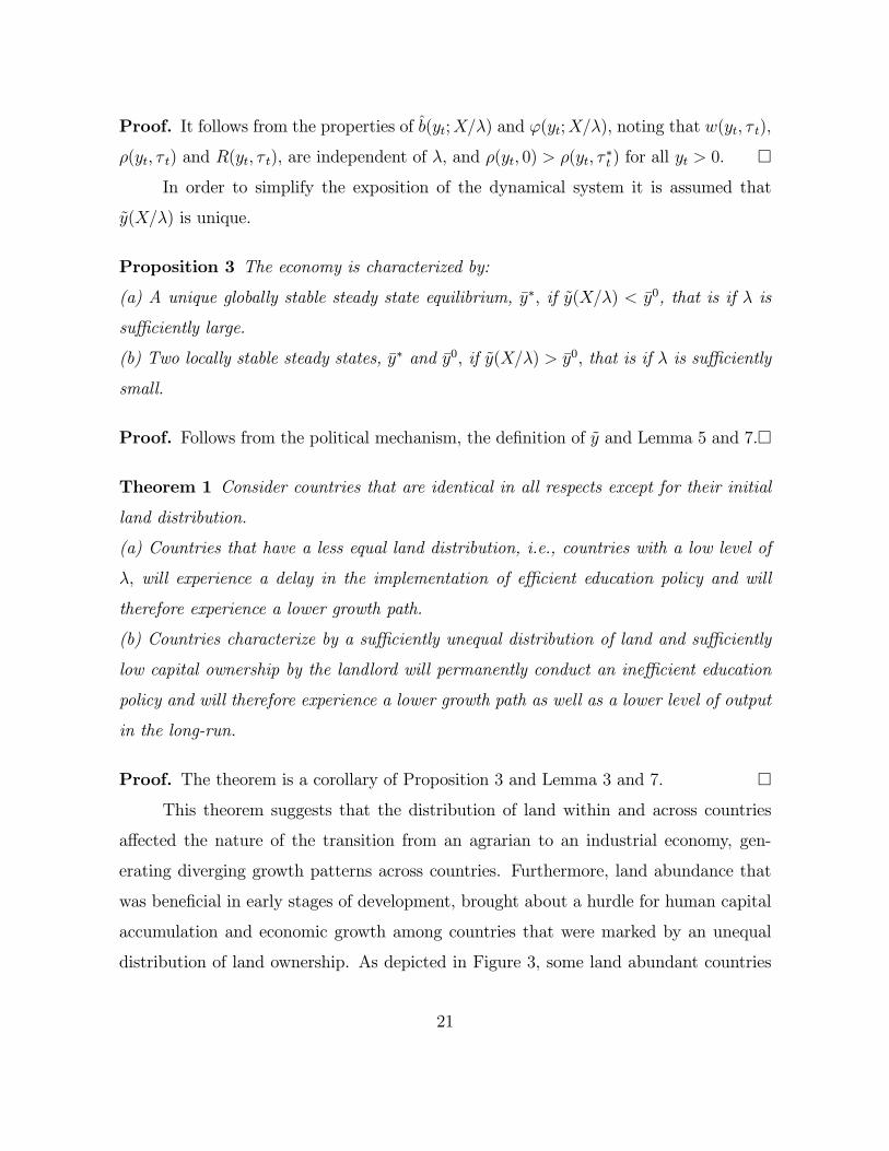
Proposition 3 The economy is characterized by:

(a) A unique globally stable steady state equilibrium, y∗, if y(X/λ) < y0, that is if λ is

sufficiently large.

(b) Two locally stable steady states, y∗ and y0, if y(X/λ) > y0, that is if λ is sufficiently

small.

Proof. Follows from the political mechanism, the definition of y and Lemma 5 and 7.¤

Theorem 1 Consider countries that are identical in all respects except for their initial

land distribution.

(a) Countries that have a less equal land distribution, i.e., countries with a low level of

λ, will experience a delay in the implementation of efficient education policy and will

therefore experience a lower growth path.

(b) Countries characterize by a sufficiently unequal distribution of land and sufficiently

low capital ownership by the landlord will permanently conduct an inefficient education

policy and will therefore experience a lower growth path as well as a lower level of output

in the long-run.

Proof. The theorem is a corollary of Proposition 3 and Lemma 3 and 7. ¤This theorem suggests that the distribution of land within and across countries

affected the nature of the transition from an agrarian to an industrial economy, gen-

erating diverging growth patterns across countries. Furthermore, land abundance that

was beneficial in early stages of development, brought about a hurdle for human capital

accumulation and economic growth among countries that were marked by an unequal

distribution of land ownership. As depicted in Figure 3, some land abundant countries

21

which were associated with the club of the rich economies in the pre-industrial revolu-

tion era and were characterized by an unequal distribution of land, were overtaken in

the process of industrialization by land scarce countries. The qualitative change in the

role of land in the process of industrialization has brought about changes in the ranking

of countries in the world income distribution.

4 Evidence from the US High School Movement

The central hypothesis of this research, that land inequality adversely affected the timing

of education reform, is examined empirically utilizing variations in public spending on

education across states in the US during the high school movement. Historical evidence

from the US on education expenditures and land ownership in the period 1880-1950

suggests that land inequality had a significant adverse effect on the timing of educational

reforms during the high school movement in the United States.

4.1 The US High School Movement 1910-1940

The qualitative changes in the education structure in the United States during the pe-

riod 1900-1950 and the variations in the timing of these education reforms across states

provides a potentially fertile setting for the test of the theory.

During the time period 1910-1940, the education system in US underwent a major

transformation, from an insignificant secondary education to a nearly universal secondary

education.16 As established by Goldin (1998) in 1910, high school graduation rates were

about 9-15% in the Northeast and the Pacific regions and about 4% in the South. By

1950, graduation rates were nearly 60% in the Northeast and the Pacific regions, and

about 40% in the South. Furthermore, Goldin and Katz (1997) document significant

variation in the timing of these changes and their extensiveness across regions states.

The average real expenditure for education per child rose by 127% in the period 1900-

1920 and by 186% in the period 1920-1950 due to widening enrollment as well as the

16See the comprehensive studies of Goldin (1998, 1999) and Goldin and Katz (1997)

22

higher cost associated with high school education.17

The high school movement and its qualitative effect on the structure of educa-

tion in the US reflected an educational shift towards non-agricultural learning that is

at the heart of the proposed hypothesis. The high school movement was undertaken

with thought towards building a skilled work-force for the services and manufacturing

sectors. As argued by Goldin (1999), “American high schools adapted to the needs of

the modern workplace of the early twentieth century. Firms in the early 1900s began

to demand workers who knew, in addition to the requisite English, skills that made

them more effective managers, sales personnel, and clerical workers. Accounting, typing,

shorthand, algebra, and specialized commercial courses were highly valued in the white-

collar sector. Starting in the late 1910s, some of the high-technology industries of the

day, such as chemicals, wanted blue-collar craft workers who had taken plane geometry,

algebra, chemistry, mechanical drawing, and electrical shop.”

Goldin and Katz (1997) exploit the significant differences in high school graduation

and attendance rates across states in order to examine the factors that were associated

with high levels of secondary education. They find that states in the U.S. that were

leaders in secondary education had high and equally distributed income and wealth and

that homogeneity of economic and social conditions were conducive to the establishment

of secondary education.

4.2 Data

In light of the proposed theory, we exploit variations in the public expenditure on edu-

cation across states in the US to examine the effect of land inequality on the high school

movement.

The historical data that is utilized in this study is gathered from several sources.

The variables, their sources, and their method of construction are reported in the Ap-

pendix.

17Goldin (1997) estimates that the cost of educating a high-school student is twice that of anelementary-school student.

23

• Income across states over this period is measured using estimates provided byEasterlin (1957) for 1900, 1920 and 1950. As these are the only years with available

income estimates, we will be limited to consideration of these years alone.

• The characterization of the timing of the high school movement is based on theclassification of Goldin (1998). As is reflected from their study, in 1900 the high-

school movement has just barely begun, by 1920 it had been well underway, and

by 1950 most of the changes in secondary education had been completed.

• In order to capture the effect of land inequality on the high school movement, weexamine the effect of the land inequality prior to the onset on the process on the

variations in the high school movement across states. The US census of 1880 is

therefore used in order to construct the Gini coefficient on land distribution.

4.3 Testable Predictions

According to the proposed theory, the nature of the relationship between land inequality

and public expenditure on education changes over time as states develop. In early stages

of development (i.e. prior to the onset of the high school movement in about 1910), the

level of development of each state does not necessitate investment in high school educa-

tion. Hence, land inequality would be expected to have limited effect on the educational

expenditures, and variations in educational expenditures would reflect mostly differences

in income across states. In later stages, however, as argued by Goldin (1999), high school

education was needed in order to produce skilled worker for the industrial and the ser-

vice sectors. At this stage, due to the lower complementarity of high school education

with the agricultural sector, the concentration of land would be expected to adversely

affect educational expenditure, and variation across states reflected variations in land

inequality as well as in income across states. Ultimately, as the necessary skills were

formed by 1940, variations in educational expenditures across states would be expected

to reflect mostly variations in income.

Hence, in the context of the available data, the prediction of the theory is that:

24

(a) There exits an insignificant relationship between initial land conditions and education

expenditures in either 1900 or in 1950, controlling for income.

(b) There exist a significant negative relationship between land inequality and education

expenditures in 1920, controlling for income.

4.4 Empirical Specification and Results

The empirical analysis is based on simple cross-sectional OLS regressions of states in

each of the years 1900, 1920, and 1950.18 Expenditure on education per child is the

dependent variable in each case. Income per capita in the years 1900, 1920 and 1950,

respectively, and the Gini coefficient for farm size distribution in 1880 are included as

explanatory variables. Land inequality in 1880, rather than the contemporary measure

of land inequality, is used for each of the 3 time periods, in order to capture the long-term

impacts of initial land inequality and to avoid the endogeneity associated with changes

in land distribution over time.

In addition we include the following controls: value per farm in 1880, the interaction

of value per farm with the Gini coefficient, the percentage of population that is black,

the percentage of population that is urban, and a dummy variable indicating if a state

is in the West.19

In order to separate the effect of land inequality from other characteristics of land,

“value per farm” and in some specifications its interaction with land inequality are

included as a control variables. The percent of the population that resides in an urban

environment is included to control for several possible influences: (a) economies of scale in

education that are more pronounced in urban areas, (b) variations in teacher salaries and

18It should be noted that another avenue of empirical investigation would be to examine the differ-ences in land conditions within states over time and their impacts on education expenditures. Thisresearch avenue, however, would generate severe problems of endogeneity. Furthermore, variations inland inequality over time within states are smaller than that across states at any given time and are toosubtle to offer much explanatory power.19Data on Income inequality in the US over this period is not available and thus is not part of our

control variables. Goldin and Katz (1997) constructed a proxy for wealth inequality across states in thisperiod based on the number of car per capita.

25

thus educational expenditures vary between rural-intensive and urban-intensive states,

and (c) the increased demand for education in urban-intensive states.

The dummy variable for the West is designed to capture the westward expansion

of settlements in the US. During the early part of the period of study, the western

states were relatively new to the U.S. and very lightly populated.20 Easterlin (1961)

describes the western economy having two characteristics. The first is a high portion of

the workforce in mining as opposed to agriculture or manufacturing,21 the second is a

very low dependency ratio. The West dummy is designed to capture differential effects

that can be attributed to these influences. As will become apparent, this control does not

affect the qualitative results. The percentage of population that is black is designed to

capture the differential effects of racial policies on educational expenditures or lingering

effects of Reconstruction.

Tables 2-4 report the outcome of the cross-sectional regressions for each of the years

1900, 1920 and 1950. Column (1) in each table shows the simple regression of expenditure

per child on income per capita. In 1900, the R-squared of this regression is roughly 85%.

In contrast, in 1920 the R-squared of the same regression is only 43%. Hence, in 1920,

there are wide differences in education expenditure beyond those explained simply by

income per capita. As is apparent from columns (4)-(6) land conditions are one of the

significant determinants of the variations in educational expenditure differences in 1920.22

Columns (2) and (3) in each table include further controls for urbanization, percent-

age black, and the west dummy. The effect of the percentage of black in the population

on expenditures per child is significantly negative under some specifications and insignif-

icant in all others. This is likely to be an outcome of the low enrollment rates of black

students, as well as the under-funding of black schools across the southern states. The

20Their low population density would potentially raise the amount of resources necessary to educatechildren to the same level as a state further east with higher population and smaller distances to cover.This is particularly important given the rising prevalence of rural busing in this period.21Although the complementarity between human capital and the agricultural and the mining sectors

are rather similar, land inequality does not capture the concentration of ownership in the mining sector.22For reasons explained in the Appendix, the 1900 regression includes only 43 states while the 1920

and 1950 regressions included 45 states. Restricting the 1920 and 1950 regressions to the same 43 statesas in 1900 has no effect on the results.

26

west dummy has a significant positive impact in both 1920 and 1950. This is consistent

with the findings of Goldin (1999) that enrollment rates in the west were generally higher

than in most other areas of the U.S.

The effect of land inequality on educational expenditure, controlling for other land

characteristics, is captured in columns (4)-(6) of Tables 2-4. As depicted in Table 2,

for the year 1900, land inequality has an insignificant effect on educational expenditure,

consistently with the theory’s testable predictions. However, as depicted in Table 3 for

the year 1920, and consistently with the testable predictions, land inequality as captured

by the Gini index on farm size in 1880, has a significant negative effect in all specifications.

In the year 1950, as depicted in Table 4, the impacts of land inequality on educational

expenditure is insignificant. Consistently with the testable predictions, once the high

school movement had been completed, the significant negative impact of land inequality

seen in 1920 is no longer present.23

It is interesting to note that as is apparent from all columns of Tables 2-4, the

positive effect of income per capita on educational expenditure increases over the entire

period. Hence, consistent with the proposed theory, land inequality determines the

timing of educational reforms, but income per capita determines the level of educational

expenditures. The rising importance of education over the period 1900-1950 magnified

the role of income per capita in the determination of variations in educational expenditure

across states.

Interestingly, the inclusion of land characteristics removes much of the significance

and size of the coefficient on the percentage of black in the population. It appears

that some of the racial differences in education outcomes worked through the poor land

distributions left behind by the plantation system in the south. (See Margo [1990] for

further discussion of the relationship between race and education in the South).

23The results for 1920 are consistent with the finding of Goldin and Katz (1997) that inequalityis associated with poor education outcomes during the high school movement. The proposed theoryidentifies an explicit mechanism through which land inequality adversely affected education outcomes.

27

5 Concluding Remarks

The proposed theory suggests that land inequality affected the nature of the transition

from an agrarian to an industrial economy generating diverging growth patterns across

countries. Land abundance, which was beneficial in early stages of development, gen-

erated in later stages a hurdle for human capital accumulation and economic growth

among countries in which land ownership was unequally distributed. The qualitative

change in the role of land in the process of industrialization affected the transition to

modern growth and has brought about changes in the ranking of countries in the world

income distribution. Some land abundant countries that were associated with the club

of the rich economies in the pre-industrial revolution era and were marked by an un-

equal distribution of land, were overtaken in the process of industrialization by land

scarce countries and were dominated by other land abundant economies in which land

distribution was rather equal.

The central hypothesis of this research that land inequality adversely affected the

timing of education reform is examined empirically, utilizing variations in public spending

on education across states in the US during the high school movement. Historical evi-

dence from the US on education expenditures and land ownership in the period 1880-1950

suggests that land inequality had a significant adverse effect on the timing of educational

reforms during the high school movement in the United States.

The theory abstracts from the sources of distribution of population density across

countries in the pre-industrialization era. The Malthusian mechanism, that positively

links population size to effective resources in each region, suggests that the distribution

of population density in the world economy should reflect in the long run the distribu-

tion of productive land across the globe. Hence, one could have argued that significant

economic variations in effective land per capita in the long run are unlikely. Never-

theless, there are several sources of variations in effective resources per-capita in the

pre-industrial world. First, due to rapid technological diffusion across countries and con-

tinents in the era of “innovations and discoveries” (e.g., via colonialism) population size

28

in the technologically receiving countries has not completed their adjustment prior to

industrialization, and population density in several regions were therefore below their

long-run level. Second, inequality in the distribution of land ownership within countries

(due to geographical conditions, for instance) prevented population density from fully

reflecting the productivity of land. Variations in population density across the globe

may therefore reflect variations in climate, settlement date, disease, colonization, and

inequality.

In contrast to the recent literature that attempts to disassociate the role of geog-

raphy and institutions in economic development, the theory suggest that geographical

conditions and institutions are intimately linked. Geographical conditions that were as-

sociated with increasing returns in agricultural, or in the extraction of natural resources

led to the emergence of a class of wealthy landlords that ultimately affected adversely the

implementation of an efficient institution of public education. Furthermore, geograph-

ical conditions were the prime determinant of the timing of the agricultural revolution

[Diamond (1997)] and due to the interaction between technological progress and pop-

ulation growth [Malthus (1789) and Boserup (1965)] the cause of variation in the level

of technology and population density, in geographically isolated regions despite similar

levels of output per capita. Hence, the link that was created between geographically

isolated areas in the era of discoveries, and the associated diffusion of technology, gen-

erated geographically-based variations in effective land per capita, that according to the

proposed theory led to the implementation of different institutions of public education.

The paper implies that differences in the evolution of social structures across coun-

tries may reflect differences in land abundance and its distribution. In particular, the

dichotomy between workers and capitalists is more likely to persist in land abundant

economies in which land ownership is unequally distributed. As argued by Galor and

Moav (2000), due to the complementarity between physical and human capital in produc-

tion, the Capitalists were among the prime beneficiaries of the accumulation of human

capital by the masses. They had therefore the incentive to financially support public

education that would sustain their profit rates and would improve their economic well

29

being, although would ultimately undermine their dynasty’s position in the social ladder

and would bring about the demise of the capitalist-workers class structure. As implied

by the current research, the timing and the degree of this social transformation depend

on the economic interest of landlords. In contrast to the Marxian hypothesis, this paper

suggests that workers and capitalists are the natural economic allies that share an inter-

est in industrial development and therefore in the implementation of growth enhancing

universal public education, whereas landlords are the prime hurdle.

30

Appendix - Data Sources

Education Expenditures - This is obtained from the Historical Statistics of the United

States for 1920 and 1950, and from the U.S. Bureau of Education, Report of the Com-

missioner of Education for 1900. These expenditures are reported in current dollars,

and are converted to 1929 dollars to match the income per capita estimates.

Expenditure per child - The number of relevant children in a year is taken from the U.S.

Census. The relevant age ranges are 5-20 years in 1900, 7-20 years in 1920, and 5-19

years in1950. Although, the age ranges in each year are not consistent, we assume that

they remain comparable over time. Furthermore, it should be noted that since we are not

comparing expenditure per child across periods, these differences in reference population

are not significant.

Value per farm - Obtained from the U.S. Census in the relevant year. The exact measure

is the value of land and land improvements (in dollars) for each state. This value is

divided by the number of farms in order to obtain the value per farm.

Gini coefficient of farm distribution - This measure was constructed for each year from

farm distribution data in the U.S. Census. For 1950 and 1920, the Census reports the

distribution of number of farms and total acreage of farms by bin size. This allows

for a straightforward estimation of a Gini coefficient. The bins used in 1950 are more

refined than the ones in 1920. In 1900 and 1880, the Census only reports the distribution

of number of farms, not their total acreage. In order to estimate a Gini, assumptions

must be made regarding the average size of a farm within each bin. For this, we turn

to the 1920 data as a guide. In most cases, the average farm size is very close to

the average expected if farms were distributed uniformly over the bin (for example, the

average farm size in 1920 in the 20-50 acre bin is close to 35 acres). Therefore, in 1880

we use the average size expected in each bin as the actual average size in each bin. The

only remaining complication is in the case where the bin for farms greater than 1000

acres. We assume that the average size of farms in this bin in 1880 is 1800 acres. These

values are lower than that in 1920 (2500 acres), but when used these values make the

31

total acreage across all bins come out very closely to the actual total farmland acreage

across states. Once these assumptions are made, Gini coefficients can be estimated for

1880. Full data concerning the calculation of these Gini coefficients is available from

the authors upon request.

Percent black - This variable is taken from the U.S. Census in the relevant years.

West Dummy - This variable equals 1 for the following states: Arizona, California,

Colorado, Idaho, Montana, Nevada, New Mexico, Oregon, Utah, and Washington, and

is 0 for all others states.

Income per capita - These are estimates by Easterlin from Population Redistribution and

Economic Growth: United States, 1870-1950, edited by Kuznets and Thomas (1957).

See their work for descriptions of how this data is constructed.

Excluded states - In the regressions presented, the number of states was either 43 or 45.

States that were excluded were generally not part of the U.S. in the time period or had

serious data issues (particularly in 1880 or 1900). Those states excluded in the 1900

regressions are: Alaska, Arizona, Hawaii, New Mexico, North Dakota, Oklahoma, and

South Dakota. Those states excluded from the 1920 and 1950 regressions are Alaska,

Hawaii, North Dakota, Oklahoma, and South Dakota.

Percent Urban - The fraction of the population residing in urban areas, where urban

area is defined as any city/town with more than 4,000 people. It is calculated based on

the corresponding U.S. Census.

32

References

[1] Acemoglu, D. and S. Johnson, Robinson, J. A (2002), “Reversal of Fortune: Geog-

raphy and Institutions in the Making of the Modern World Income Distribution ”

Quarterly Journal of Economics, 117.

[2] Besley T, Burgess R (2000) “Land reform, poverty reduction, and growth: Evidence

from India” Quarterly Journal of Economics 115 (2): 389-430 May.

[3] Boserup, E., (1965). The Conditions of Agricultural Progress Aldine Publishing

Company, Chicago, Il.

[4] Benabou, R. (2000), “Unequal Societies: Income Distribution and the Social Con-

tract, American Economic Review, 90, 96-129.

[5] Bertocchi, G.,. (2002), “The Law of Primogeniture and the Transition from Landed

Aristocracy to Industrial Democracy,” University of Medena.

[6] Caselli, F., and W.J. Coleman, (2001), “The US structural transformation and

regional convergence: A reinterpretation,” Journal of Political Economy, 109, 584-

616

[7] Coatsworth, John H. “Notes on the Comparative Economic History of Latin Amer-

ica and the United States.” In Development and Underdevelopment in America,

Bernecker, Walther and Hans Werner Tobler, Eds. Walter de Gruyter. 1993

[8] Deninger K, and Squire, L (1998), “New Ways of Looking at Old Issues: Inequality

and Growth”, Journal of Development Economics, 57, 259-287.

[9] Diamond, J. (1997).Guns, Germs, and Steel: The Fates of Human Societies.

[10] Easterlin, Richard A.. 1957 ”Regional Growth of Income: Long Term Tendencies.”

in Population Redistribution and Economic Growth: United States, 1870-1950, Vol.

2: Analysis of Economic Change. Edited by Simon Kuznets, Ann Ratner Miller,

and Richard A. Easterlin. American Philosophical Society: Philadelphia.

[11] Eckert, C.J. Korea Old and New: A History. Seoul. 1990.

[12] Engerman, Stanley L., and Kenneth L. Sokoloff. 1997. “Factor Endowments, Insti-

tutions, and Differential Paths of Growth Among New World Economies: A View

from Economic Historians of the United States.” In Stephen Haber, ed., How Latin

America Fell Behind. Stanford, Calif.: Stanford University Press

33

[13] Estevo, Gustavo. The Struggle for Rural Mexico. Bergin and Garvey, South Hadley,

MA. 1983.

[14] Fox. “Agricultural Wages in England.” Journal of the Royal Statistical Society, Vol.

66. London. 1903.

[15] Galor, O. and Zeira, J. (1993), ‘Income Distribution and Macroeconomics’, Review

of Economic Studies, vol. 60, pp. 35-52.

[16] Galor, Oded and Weil, David N. (2000) “Population, Technology and Growth: From

the Malthusian Regime to the Demographic Transition,” American Economic Re-

view, 90(4), pp. 806-828.

[17] Galor, O. and O. Moav (2002), “Natural Selection and the Origin of Economic

Growth,” Quarterly Journal of Economics, 117.

[18] Galor, O. and O. Moav (2000), Das Human Kapital”.

[19] Gerber, J., (1991), “Public-School Expenditures in the Palntation Sates, 1910,”

Explorations in Economic History, 28, 309-322.

[20] Goldin, C., (1999) “Egalitarianism and the Returns to Education During the Great

Transformation of American Education”. The Journal of Political Economy, 107(6):

S65-S94.

[21] Goldin, C., (1998), “America’s Graduation from High School: The Evolution and

Spread of Secondary Schooling in the Twentieth Century,” Journal of Economic

History. 58: 345-74.

[22] Goldin, C. and L. F. Katz (1998), ‘The Origins of Technology-Skill Complementary’,

Quarterly Journal of Economics, vol. 113, pp.693-732.

[23] Goldin, C. and Katz, L. F., (1997), ”Why the United States Led in Education:

Lessons from Secondary School Expansion, 1910 to 1940.” NBER Working Paper

no. 6144.

[24] Gylfason T. (2001).“Natural Resources, Education, and Economic Development,”

European Economic Review (45)4-6 847-859.

[25] Inter-university Consortium for Political and Social Research. Historical, Demo-

graphic, Economic and Social Data: The United States, 1790-1970 [Computer file].

Ann Arbor, MI.

34

[26] Kuznets, S. (1955), ‘Economic Growth and Income Equality’, American Economic

Review, vol. 45, pp. 1-28.

[27] Lane P.R. and A. Tornel (1996). “Power, Growth and the Voracity Effect,” Journal

of Economic Growth, 1, 213-242.

[28] Loveman, Brian. Allende’s Chile: Political Economy of the Peaceful Road to Disas-

ter. Latin American Studies Association. 1974.

[29] Lucas, Robert E. , Jr. (2000). “Some Macroeconomics for the 21st Century,” Journal

of Economic Perspectives, 14, 159-168.

[30] Maddison, Angus. Monitoring the World Economy 1820-1992. OECD. 1995

[31] Margo, Robert A.. 1990. Race and Schooling in the South, 1880-1950: An Economic

History. University of Chicago Press: Chicago.

[32] Mokyr, Joel. The Lever of Riches, New York: Oxford University Press, 1990.

[33] North, Douglas C. (1981) Structure and Change in Economic History, W.W. Norton

& Co., New York.

[34] Perotti, R. (1996), ‘Growth, Income Distribution, and Democracy: What the Data

Say’, Journal of Economic Growth, vol. 1, pp. 149-87.

[35] Persson, T. and G. Tabellini, Political Economics: Explaining Economic Policy,

MIT Press 2000.

[36] Pritchett, L. (1997), “Divergence, Big Time,” Journal of Economic Perspectives,

11, 3-18.

[37] Quah, D. (1997). “Empirics for Growth and Distribution: Stratification, Polariza-

tion and Convergence Clubs,” Journal of Economic Growth, 2, 27-60.

[38] Ringer, F. (1979) Education and Society in Modern Europe, Indiana University

Press, Bloomington.

[39] Sachs, Jeffrey and Andrew M. Warner. (1995). “Natural Resource Abundance and

Economic Growth.” NBER Working Paper 5398.

[40] Sokoloff, Kenneth. “Institutions, Factor Endowments, and Paths of Development in

the New World.” Villa Borsig Workshop Series. www.dse.de/ef/instn/sokoloff.htm.

2000.

35

[41] Rodrigues, F. and Sachs, J.D. (1999) “Why do Resource Abundance Economies

Grow More slowly?” Journal of Economic Growth, 4, 277 - 304.

[42] U.S. Bureau of Education. 1870-1950. Report of the Commissioner of Education.

Government Printing Office: Washington D.C..

[43] U.S. Bureau of the Census. 1989. Historical Statistics of the United States: Colonial

Times to 1970. Kraus International Publications: White Plains, NY.

[44] U.S. Department of Agriculture, Profile of Hired Farmworkers, 1998 Annual Aver-

ages.

[45] Wright, D.G. (1970) Democracy and Reform 1815-1885, Longman, London.

[46] Yoong, D.J. 2000 “Land Reform, Income Redistribution, and Agricultural Produc-

tion in Korea.” Economic Development and Cultural Change. 48(2)

36

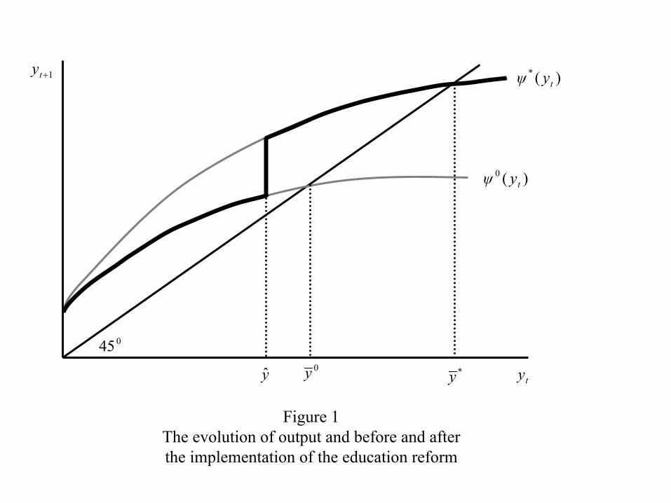
Figure 1The evolution of output and before and afterthe implementation of the education reform

1+ty

ty*y0yy

045

)(*tyψ

)(0tyψ

ty

λβ /ty

)(ˆ tyb0y

0bb

0yy

*y

Figure 2The Evolution of output and Landowner’s bequestprior to the implementation of education reform

Figure 3Overtaking – country A is relatively richer in land, however, due to land inequality it fails to implement efficient schooling and is overtaken by country B. Alternatively, for a lower degree of inequality, country A will eventually implement education reforms and ultimately takeover country B (not captured in the figure).

1+ty

tyBy ][ *Ay ][ 0By

045

Btyψ )]([ *

Btyψ )]([ 0

Ay

Atyψ )]([ 0

By0Ay0

Table 1: GDP per Capita Relative to the US

Country Note 1870 1900 1913 1930 1940 1950 1960 1994Australia 154.70 104.96 103.73 77.04 84.64 75.40 76.29 75.80USA 100.00 100.00 100.00 100.00 100.00 100.00 100.00 100.00New Zealand 126.78 105.47 97.57 80.14 90.23 88.74 84.79 66.84UK 132.80 112.13 94.82 83.52 93.27 71.52 76.57 72.54Canada 65.93 67.33 79.39 73.28 72.47 73.61 75.57 81.31Switzerland 88.40 86.21 79.27 99.04 89.90 93.38 109.77 92.29Belgium 107.45 89.16 78.39 78.34 63.62 55.84 60.56 76.32Netherlands 107.45 86.25 74.43 87.89 67.17 61.11 72.23 76.00Germany 77.86 76.51 72.23 65.10 79.01 44.72 75.61 84.62Argentina 53.36 67.29 71.55 65.59 59.33 52.09 49.66 37.10Denmark 78.43 70.85 70.93 82.60 70.13 69.81 75.73 85.54Austria 76.31 70.83 65.72 58.04 56.78 38.97 58.62 76.59France 75.62 69.56 65.05 72.17 57.05 54.54 66.76 79.61Sweden 67.72 62.52 58.34 63.30 69.22 70.39 77.62 74.04Ireland *** 72.16 60.91 51.50 46.35 44.40 36.75 39.02 55.94Chile 47.58 50.01 50.53 46.44 39.98 38.45 34.40Italy 59.71 42.63 47.24 45.88 48.86 35.78 51.72 72.68Norway 53.03 43.02 42.87 54.29 52.98 51.91 58.51 81.40Spain *** 56.00 49.80 42.49 47.38 28.81 25.04 30.71 55.58Finland 45.05 39.55 38.63 41.62 44.57 43.15 54.06 65.48Greece *** 30.54 38.36 38.86 20.38 28.63 45.04Mexico 28.90 28.25 27.64 22.04 22.17 21.78 24.85 22.59South Africa ** 27.34 23.51 23.44 15.29Philippines * 25.22 26.72 21.33 13.51 13.29 9.81Portugal *** 44.16 34.38 25.51 24.69 24.32 22.27 27.65 49.11Japan 30.16 27.71 25.14 28.62 39.40 19.57 34.66 86.42Colombia 23.75 23.29 23.70 27.00 21.82 22.33 23.74Venezuela 20.04 20.80 55.37 57.64 77.55 86.89 37.17Peru 19.95 19.54 22.78 25.98 23.64 27.01 14.32Turkey *** 18.45 15.37 19.36 13.57 16.09 18.90S. Korea * 20.75 17.86 18.86 23.50 9.15 11.63 44.35Indonesia * 26.74 18.19 17.28 19.26 16.19 9.13 10.10 12.18Thailand * 29.18 19.82 15.94 11.86 8.86 9.19 20.80

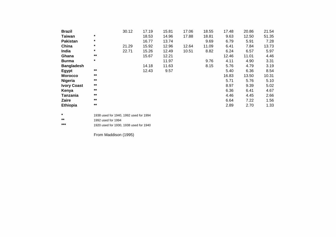
Brazil 30.12 17.19 15.81 17.06 18.55 17.48 20.86 21.54Taiwan * 18.53 14.96 17.88 18.81 9.63 12.50 51.35Pakistan * 16.77 13.74 9.69 6.79 5.91 7.28China * 21.29 15.92 12.96 12.64 11.09 6.41 7.84 13.73India * 22.71 15.26 12.49 10.51 8.82 6.24 6.57 5.97Ghana ** 15.67 12.21 12.46 11.01 4.46Burma * 11.97 9.76 4.11 4.90 3.31Bangladesh 14.18 11.63 8.15 5.76 4.79 3.19Egypt ** 12.43 9.57 5.40 6.36 8.54Morocco ** 16.83 13.50 10.31Nigeria ** 5.71 5.76 5.10Ivory Coast ** 8.97 9.39 5.02Kenya ** 6.36 6.41 4.67Tanzania ** 4.46 4.45 2.66Zaire ** 6.64 7.22 1.56Ethiopia ** 2.89 2.70 1.33

* 1938 used for 1940, 1992 used for 1994** 1992 used for 1994*** 1920 used for 1930, 1938 used for 1940

From Maddison (1995)

Table 2 - 1900

(1) (2) (3) (4) (5) (6)Exp/Child Exp/Child Exp/Child Exp/Child Exp/Child Exp/Child

Exp Variable in 1900 in 1900 in 1900 in 1900 in 1900 in 1900Income per capita 0.0515 ** 0.0473 ** 0.0310 ** 0.0253 ** 0.0250 ** 0.0344 **(in 1900) (15.41) (9.25) (3.90) (2.98) (2.88) (6.00)

Percent Urban 4.3893 6.9113 6.0582 6.4669 1.4306(in 1900) (0.96) (1.36) (1.07) (1.07) (0.29)

Percent Black -16.3616 ** -10.3195 * -9.8481 -11.0278 *(in 1900) (3.81) (1.72) (1.53) (1.70)

West Dummy 2.3209 3.6219 3.5902(1.03) (1.47) (1.44)

Gini of farm size -10.3157 -12.9530 8.4675(in 1880) (1.22) (0.90) (0.59)

Value per farm 0.0009 0.0005 0.0003(in 1880) (1.67) (0.26) (0.13)

Value x Gini 0.0009 0.0013(in 1880) (0.23) (0.30)

Constant -3.6445 ** -3.1346 ** 4.6074 * 7.8658 ** 9.0543 5.8511(2.39) (1.98) (1.79) (1.98) (1.37) (0.93)

Adj R-squared 0.8492 0.8356 0.8764 0.8813 0.8779 0.8741

total observations 43 43 43 43 43 43

Method OLS OLS OLS OLS OLS OLS

Absolute values of t-ratios are given in parentheses** indicates significance at 5%* indicates significance of 10%

Table 3 - 1920



Percent Urban -63.2109 ** -29.7652 ** -30.6677 ** -28.4024 ** -54.8714 **(in 1920) (4.33) (2.10) (2.32) (2.08) (3.67)

Percent Black -55.3037 ** -13.1901 -12.9234 -37.8683 *(in 1920) (3.65) (0.71) (0.69) (1.74)

West Dummy 17.2578 ** 21.8742 ** 21.1836 **(3.49) (4.67) (4.41)

Gini of farm size -58.5236 ** -74.0453 ** -68.2059 **(in 1880) (3.30) (2.68) (2.03)

Value per farm -0.0004 -0.0040 -0.0088(in 1880) (0.25) (0.78) (1.46)

Value x Gini 0.0077 0.0165(in 1880) (0.74) (1.34)

Constant -4.7883 -8.9532 22.0132 ** 34.8223 ** 42.7961 ** 43.2102 **(0.58) (1.28) (2.52) (3.76) (3.00) (2.48)

Adj R-squared 0.4269 0.5941 0.7561 0.8024 0.8000 0.7031




Table 4 - 1950



Percent Urban -50.8679 * -2.7542 -15.0726 -9.9397 -53.8111 *(in 1950) (1.79) (0.12) (0.61) (0.40) (1.92)

Percent Black 25.8008 16.4902 24.9224 -48.8358(in 1950) (0.97) (0.48) (0.73) (1.31)

West Dummy 37.6302 ** 36.0743 ** 33.5774 **(6.09) (5.00) (4.55)

Gini of farm size 11.1579 -37.1389 -13.2087(in 1880) (0.39) (0.81) (0.24)

Value per farm 0.0031 -0.0078 -0.0174 *(in 1880) (1.32) (0.93) (1.74)

Value x Gini 0.0224 0.0415 **(in 1880) (1.35) (2.09)

Constant 0.3783 3.9067 -2.9764 1.2903 19.9228 24.2772(0.03) (0.29) (0.21) (0.07) (0.87) (0.86)

Adj R-squared 0.6281 0.6463 0.8102 0.8102 0.8142 0.7178




land inequality and the origin of divergence and

Documents