Land Reform and Productivity: A Quantitative Analysiswith Micro Data†

Tasso AdamopoulosYork University

Diego RestucciaUniversity of Toronto

November 2013 - Preliminary and Incomplete

Abstract

We assess the effects of a major land policy change on farm size and agricultural productivity,using a quantitative model and micro-level data. In particular, we study the 1988 land reform inthe Philippines, which was an extensive land redistribution program that imposed a ceiling of 5hectares on all land holdings while at the same time severely restricting the transferability of theredistributed farm lands. Our micro data allow us to track a set of Philippine farmers, before andafter the reform, offering rich input and output information at the parcel-level. This data allows usto obtain precise measures of farm-level productivity, and study how the choices of farmers changedfollowing the reform. We decompose the change in aggregate agricultural productivity, following thereform, into: (a) a reallocation effect, whereby farming activity is shifted from large farms to smallfarms and (b) a within-farm effect. We find that the source of the within-farm effect is a changein the crop mix between cash crop and food crops. We develop a quantitative model with a non-degenerate distribution of farm sizes that features an occupational-choice decision for the farmer.A farm operator chooses between two technologies: a “cash crop” and a “food crop” technology.The cash crop technology has higher TFP but requires a higher fixed cost. A land reform reducesaggregate agricultural productivity not only by reallocating resources from large/high productivityfarms to small/low productivity farms, but also by altering how farmers sort themselves acrosstechnologies. We calibrate the model to the agricultural sector of the Philippines before the reform.We find that the land reform reduces average farm size by 9% and agricultural productivity by 5%.From the overall productivity effect, 60% is accounted for by the misallocation channel, while therest by the selection channel. We also find that other changes occurring alongside the reform canmask the effects of the reform in time series data.

JEL classification: O11, O14, O4.Keywords: agriculture, misallocation, within-farm productivity growth, land reform.

†Contact: Tasso Adamopoulos, tasso@econ.yorku.ca; Diego Restuccia, diego.restuccia@utoronto.ca

1

1 Introduction

A key challenge in the literature on misallocation and development is to measure quantitatively how

specific establishment-level policies affect productivity at the industry level. For the very poor coun-

tries in particular, understanding how farm-level policies affect aggregate agricultural productivity

is an especially pressing issue. This is because the poorest countries: (a) are particularly unproduc-

tive in agriculture and devote a lot of resources to it, when compared to rich countries (Restuccia,

Yang, and Zhu, 2008) and (b) on average undertake farming at a much smaller operational scale

than rich countries (Adamopoulos and Restuccia, forthcoming).

The purpose of this paper is to assess the effects of a major land-policy change on farm size and

agricultural productivity, using a quantitative model and micro-level data. In particular, we study

the 1988 land reform in the Philippines, known as the Comprehensive Agrarian Reform Program

(CARP). CARP was an extensive land redistribution program that imposed a ceiling of 5 hectares on

all land holdings, while at the same time severely restricting the transferability of the redistributed

farm lands. We combine two sources of micro data to study the size and productivity effects of the

land reform: (a) Decennial Agricultural Census Data, which offer a complete enumeration of farms,

land and labor inputs at the farm level in two separate cross sections, before and after the reform;

(b) Philippines Cash Cropping Project, a panel of farm survey data, which tracks a much more

limited number of rural households before and after the reform but offers a wealth of information

on all inputs and outputs at the parcel and farm level. Combining these two sources of micro data

allows us to measure choices on farm size, input mix, output mix, and productivity changes before

and after the reform. Relative to previous studies this allows us to study the channels through

which land policy affects agricultural productivity at the industry level. In particular, we can

decompose the change in aggregate agricultural productivity into: (a) a reallocation effect, whereby

farming activity is shifted from large farms to small farms, and (b) a within-farm effect, whereby

productivity changes at the farm level over time. Given that we observe outputs and inputs as well

2

as their prices separately at the parcel level, we do not have to rely on industry deflators to compute

farm-level productivity.

A nice feature of using a panel of farm surveys is that it permits tracking a particular farmer

over time and therefore it allows the researcher to also observe the source of the within-farm effect

following the reform. Looking inside the farm, we can address whether the farmer is doing something

different after the policy change compared to before: e.g. change in the crop mix or change in the

input mix. Further, there will be farmers that were initially below the land reform ceiling (and still

are) and those that were initially above and are now brought down as a result of the reform. This

type of exercise in a given country over time controls for farmer ability and for location since land

quality and climate can be kept constant. Our data indicate a change in the crop mix between food

cropping and cash cropping, for the same set of farmers.

To study the effects of the Philippine land reform, we develop a quantitative model that builds on

the model of farm size of Adamopoulos and Restuccia (forthcoming). This is a two-sector model

of agriculture and non-agriculture that features a non-degenerate distribution of farm sizes. Farm

size is endogenized by embedding a Lucas (1978) span-of-control model of firm size in agriculture

into a standard two-sector model. The novelty of the model lies in that agricultural goods are not

produced by a representative farm but instead by farmers who are heterogeneous with respect to

their ability in managing a farm. In this model farmer-level productivity is drawn from a known

distribution but is fixed, that is the farmer cannot take any action to affect the productivity of

the farm. We extend the model of farm size in Adamopoulos and Restuccia (2011) by including

an occupational choice decision for the farmer. The farmer chooses whether to become a hired

worker or an operator of a farm, and as an operator can choose between two technologies, a “cash

crop” technology and a “food crop” technology. The cash crop technology has higher TFP but also

requires a higher fixed operating cost. The motivation for this broad technology-choice specification

is dictated by our farm survey data.

3

In this framework, in the absence of any idiosyncratic distortions the farm size distribution and the

allocation of farmers across occupations and technologies is optimal. A land reform that imposes

a ceiling reduces farm size and aggregate agricultural productivity through two channels: (1) by

reallocating resources from large/high productivity farms to small/low productivity farms - the

misallocation effect, and (2) by altering how farmers sort themselves across occupations and across

technologies - the selection effect. In particular the selection effect induced by the land reform,

consists of an increase in the number of operators and a technology switch towards the higher

productivity cash crop. Then at the sectoral level productivity drops because overall there are now

more low ability farmers operating farms, while the ones that switch to larger scale cash cropping

face a binding ceiling on their operations. Both the misallocation channel and the selection channel

reduce aggregate agricultural productivity.

We calibrate the model to the agricultural sector of the Philippine economy before the reform,

matching in particular the farm and land distributions from the survey data prior to the reform.

We discipline the parameters of the technology choice from the farm survey data, on farm cropping

patterns. In our baseline quantitative experiment we impose the land reform policy limiting farm

size to 5 hectares as if this is the only thing happening and and we study the consequences of this

policy for average farm size, aggregate agricultural productivity, and the distribution of farm-level

productivities. We find that the land reform alone reduces average farm size by 9.3% and aggregate

agricultural productivity by 5%. We then decompose the change in productivity into a reallocation

effect and a selection effect. We find that out of the 5% drop in productivity, 60% is accounted for

by the misallocation channel directly.

We also examine how farm size and productivity are affected when we combine the ceiling with

the other changes occurring alongside the reform over the same period, such as overall productivity

growth in the economy (captured by productivity growth in non-agriculture), change in land per

capita, change in the relative price of cash to food crops, crop-specific productivity changes. We

4

find that taking these changes into account can mask the effects of the land reform. As a result

when looking at times series data one might not observe the negative effect of the reform on size

and productivity. In this sense, it is useful to look at the land reform through the lens of the model,

because it allows you to disentangle the impact of the land reform from other factors.

2 Land Reforms

We focus on a specific policy that distorts farm size in a stark way: land reform. By land reform here

we mean the redistribution of land from land-rich (e.g. large landowners) to land-poor (e.g. tenants,

smallholders, landless). In practice many land reforms involved the legislation of a maximum ceiling

on land holdings, with a redistribution of the land in excess of the ceiling. Often such land reforms

were accompanied by restrictions on the land sales and land rental markets. Land reforms have

been very prevalent in developing countries in the second half of the 20th century.

In Table 1 we have compiled a set of land reforms that have been implemented since the 1950s for

countries for which we were able to obtain data. The middle column indicates the period of the land

reform. The column to the right provides the explicit legislated ceiling imposed by the reform. This

ceiling per se might not be a good description of how restrictive or binding the reform was, as these

countries differ in their pre-reform average farm size. One way to measure the restrictiveness of the

reform is to look at the ratio of the ceiling to the pre-reform average farm size. This restrictiveness

ratio varies quite a bit across reforms: e.g. 1.75 in the Philippines, 9 in Bangladesh. Of course

these reforms can also vary in the degree of enforcement. In the first column we calculate the

change in average farm size before and after the reform using census data from the World Census

of Agriculture (and where such data are absent from the respective national agricultural censuses).

What is noteworthy, is that in all these cases average farm size dropped following the reform. This

should be put in perspective, since the tendancy for average farm size is to increase over time,

5

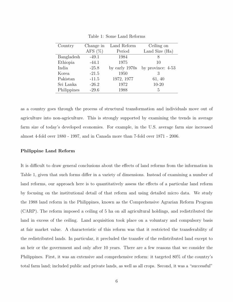
Table 1: Some Land Reforms

Country Change in Land Reform Ceiling onAFS (%) Period Land Size (Ha)

Bangladesh -49.1 1984 8Ethiopia -44.1 1975 10India -25.8 by early 1970s by province: 4-53Korea -21.5 1950 3Pakistan -11.5 1972, 1977 61, 40Sri Lanka -26.2 1972 10-20Philippines -29.6 1988 5

as a country goes through the process of structural transformation and individuals move out of

agriculture into non-agriculture. This is strongly supported by examining the trends in average

farm size of today’s developed economies. For example, in the U.S. average farm size increased

almost 4-fold over 1880 - 1997, and in Canada more than 7-fold over 1871 - 2006.

Philippine Land Reform

It is difficult to draw general conclusions about the effects of land reforms from the information in

Table 1, given that such forms differ in a variety of dimensions. Instead of examining a number of

land reforms, our approach here is to quantitatively assess the effects of a particular land reform

by focusing on the institutional detail of that reform and using detailed micro data. We study

the 1988 land reform in the Philippines, known as the Comprehensive Agrarian Reform Program

(CARP). The reform imposed a ceiling of 5 ha on all agricultural holdings, and redistributed the

land in excess of the ceiling. Land acquisition took place on a voluntary and compulsory basis

at fair market value. A characteristic of this reform was that it restricted the transferability of

the redistributed lands. In particular, it precluded the transfer of the redistributed land except to

an heir or the government and only after 10 years. There are a few reasons that we consider the

Philippines. First, it was an extensive and comprehensive reform: it targeted 80% of the country’s

total farm land; included public and private lands, as well as all crops. Second, it was a “successful”

6

reform: 80% of the targeted land had been redistributed by the early 2000s. Third, the reform was

restrictive. From the countries that we were able to obtain data for in Table 1 it was the most

restrictive, with a restrictiveness ratio of 1.75. Finally, it is a relatively recent reform, and as a

result good data exists before and after the reform.

3 Data Analysis

To study the effects of the Philippine land reform on farm size and productivity we use aggregate

and micro-level data. The aggregate sectoral data allow us to observe what has happened to farm

size and agricultural productivity for Philippine agriculture as a whole. The micro level data allow

us to conduct a deeper investigation of the sources of the changes in farm size and productivity.

We use two sources of micro-level farm data for the Philippines: (a) the decennial agricultural

censuses, and (b) the Philippines Cash Cropping Project. The decennial agricultural censuses are

undertaken by the National Statistics Office (NSO) of the Republic of the Philippines (we use the

1981 and 2002 Census of Agriculture) and provide a complete enumeration of farms covering the

entire country. Even though the census data is comprehensive it does not provide information on

outputs or other inputs (besides land and hired labor) at the farm level. In order to calculate

productivity with precision at the farm-level, in addition to the Census data, we use more detailed

survey data. In particular, we use household survey data from the International Food Policy

Research Institute (IFPRI), known as the Philippines Cash Cropping Project (PCCP) which was

conducted in the Bukidnon province on the island of Mindanao.1

1Mindanao is the second largest island (after Luzon) in the Philippines, located in the south-east of the country.Bukidnon is the food basket of the island. Compared to Luzon, Mindanao has a more even distribution of rainfallthroughout the year, is not on the path of typhoons, and has lower population density.

7

1985 1990 1995 2000 200512

13

14

15

16

17

18

19

20

Year

Re

al V

A P

er

Wo

rke

r in

Ag

ricu

ltu

re

Land Reform, 1988

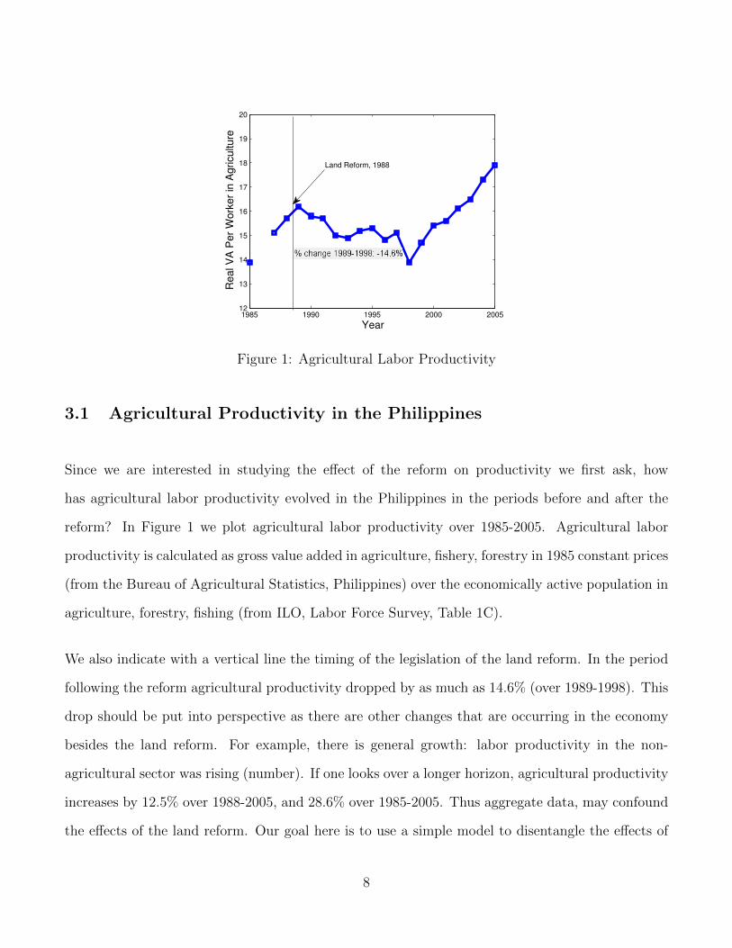
Figure 1: Agricultural Labor Productivity

3.1 Agricultural Productivity in the Philippines

Since we are interested in studying the effect of the reform on productivity we first ask, how

has agricultural labor productivity evolved in the Philippines in the periods before and after the

reform? In Figure 1 we plot agricultural labor productivity over 1985-2005. Agricultural labor

productivity is calculated as gross value added in agriculture, fishery, forestry in 1985 constant prices

(from the Bureau of Agricultural Statistics, Philippines) over the economically active population in

agriculture, forestry, fishing (from ILO, Labor Force Survey, Table 1C).

We also indicate with a vertical line the timing of the legislation of the land reform. In the period

following the reform agricultural productivity dropped by as much as 14.6% (over 1989-1998). This

drop should be put into perspective as there are other changes that are occurring in the economy

besides the land reform. For example, there is general growth: labor productivity in the non-

agricultural sector was rising (number). If one looks over a longer horizon, agricultural productivity

increases by 12.5% over 1988-2005, and 28.6% over 1985-2005. Thus aggregate data, may confound

the effects of the land reform. Our goal here is to use a simple model to disentangle the effects of

8

the reform from other changes that may be occurring along side the reform in the Philippines over

the same period.

3.2 Changes in Farm Size - Census Data

We note that in the census data a farm is an operational unit regardless of ownership or legal status.

A farm may consist of more than one parcels, as long as all are under the same management and

use the same means of production.

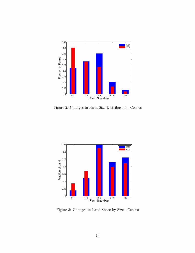
In the last decennial census before the reform (1981) average farm size was 2.85 ha. By the 2002

census (there was a decennial census in 1991 but given that the land reform had largely not been

implemented by that time we look at the next census) average farm size had dropped to 2.01 ha,

a drop of 29.6%. This drop in average scale of operation is also evident when examining the farm

size distribution in Figure 2, which shows the share of farms within each size category for 1981 and

2002. As is clear there has been a shift in the mass of farms from larger scale farms (2+ ha) to

smaller scale farms (less that 1 ha) over 1981-2002.

In Figure 3 we plot the share of farm land operated by farms within each farm size category. This

graph also indicates a shift in land mass from larger farms (2+ ha) to smaller farms (0-2 ha).

3.3 Survey Micro Data

In the PCCP survey data 448 households were interviewed in four rounds over 1984-85 (just before

the reform). Then the original households and their children were interviewed again in five rounds

(seasons) over 2002-03.2 Although the number of farms is much more limited than in the census,

2Bouis and Haddad (1990) contains a detailed description of the project and an analysis of the 1984-85 data.

9

0−1 1−2 2−5 5−10 10+0

0.05

0.1

0.15

0.2

0.25

0.3

0.35

0.4

0.45

Farm Size (Ha)

Fra

ctio

n o

f F

arm

s

1981

2002

Figure 2: Changes in Farm Size Distribution - Census

0−1 1−2 2−5 5−10 10+0

0.05

0.1

0.15

0.2

0.25

0.3

0.35

Farm Size (Ha)

Fra

ctio

n o

f L

an

d

1981

2002

Figure 3: Changes in Land Share by Size - Census

10

it tracks the same set of households before and after the reform. The survey offers a wealth of

information, with precise and detailed measurement of inputs and outputs at the parcel and farm

level.3 There are two important benefits of using this data for production-unit productivity calcu-

lations. First, in contrast to many establishment-level studies that have access only to information

on sales and input expenditures by establishment, we observe quantities and prices of outputs and

inputs separately at the parcel-level. This allows us to obtain more precise measures of real produc-

tivity without having to resort to using industry level deflators. Second, the fact that we observe

this information at the parcel level, and we know which parcels are operated by which households,

we are able to accurately aggregate productivity up to the farm-level. To appreciate the benefit

of this contrast it to many other industry studies which only observe information at the plant or

establishment level, without being able to identify the common firm to which several plants may

belong.

We use the PCCP survey data in order to understand how the land reform affects productivity at

the farm-level. In particular, how does the land reform alter the farmer’s allocation of resources

across activities within the farm? This within farm effect, in combination with the more obvious

reallocation effect, will allow us to get a better handle of the effects of the reform for agricultural

productivity in the Philippines over time.

In 1984-85, when the first rounds of the survey were conducted, the study area was primarily

engaged in corn, rice, and sugarcane production plus some other crops such as bananas, cacao,

rubber, coffee, pineapples, coconut. We group these crops into two categories based on the purpose

of production. The first category, food crops, include corn and rice, which are produced on a semi-

subsistence basis by farmers for their own consumption and for sale to the market. The second

category, cash crops, are crops for which production is undertaken on a commercial scale and its

3This survey provides rich data not only on production, but also on consumption and nutrition patterns ofhouseholds, as the primary purpose of the survey was to study the effect of agricultural commercialization onnutrition.

11

primary purpose is to sell to the market and/or export. Among cash crops, the pre-dominant one

in the study area is sugarcane and to a lesser extent coffee, coconut, and rubber. The dominance

of sugarcane production as a cash crop was facilitated by the establishment of a sugar mill in the

area named BUSCO, which provided farmers with the opportunity to switch from corn and rice

to sugarcane production. In our sample there are farms that produce exclusively food crops, those

that produce exclusively cash crops, and those that mix production between the two types.

We use our data to study the allocation of resources across cash and food crops at the farm level,

and how the land reform affects that allocation. This crop mix decision at the farm level constitutes

the “within” farm mechanism we emphasize.

To compare farm-level productivity across farms and across time (from 1984-85 to 2002-03) we use

as constant prices for all farms the average 2002-03 crop and intermediate input prices to calculate

value added. By fixing prices to their averages across farms in 2002-03, we are effectively purging

the effect of price changes from changes in value added. Thus changes in value added reflect real

changes. Productivity by farm in 1984-85 is calculated as the weighted average of productivities

over the four rounds in that first wave of the survey. Similarly, productivity by farm in 2002-03 is

calculated as the weighted average of productivities over the five seasons in this second wave of the

survey.

In order to control for farmer ability and location we only focus on the farms that are present in

both 1984-85 and 2002-03. This allows us to construct a two-year panel, with observations for the

same set of farms in each year. There are 167 farms with productivity data in both years. We group

the cash crop farms and mixed crop farms together because they are similar in their characteristics.

Thus it should be clear that the category “cash crop” farms includes both those that produce only

cash crops and those that produce cash crops and some food crops. The category “food crops”

includes those that produce only food crops. Another categorization that we will emphasize is that

between “small” - below 5 ha, and “large” - above 5 ha, where the cutoff of 5 ha is chosen to match

12

Table 2: Number of Farms By Crop and Size

1984-85 2002-03All Crops 167 167< 5 Ha 130 1415+ Ha 37 26

Cash Crops 103 123< 5 Ha 71 995+ Ha 32 24

Food Crops 64 44< 5 Ha 59 425+ Ha 5 2

the ceiling in the 1988 land reform. Table 2 reports the number of farms by crop and size in each

of the two years of the panel.

There are two shifts that occurred over time that are apparent from this table. First, a shift from

food crop farms to cash crop farms. Given that the set of farms is the same in each year, this

indicates that some farmers switched from producing food crops to cash crops.4 Second, there is a

shift from large scale farms to small scale farms. This is true for both types of crops. Interestingly,

the number of farms over 5 ha is not eliminated. This is consistent with the census data reported

above. In sum, the share of cash crop farms increased from 62% in 1984-85 to 74% by 2002-03,

while the share of small farms increased from 78% to 84% over the same period.

Table 3 displays average farm size and labor productivity by crop. Labor productivity is measured

as value added at constant 2002-03 prices over the number of work days. The number of work

days is a more precise measure of labor input as it counts how many full days are worked. This is

one of the advantages of our data as it reports days worked by task on each of the farm’s parcel.

4In 1984-85 the mixed crop farms are the biggest component of “cash crop” farms (97 out of 103). By 2002-03mixed farms still remain the largest component of cash crop farms (76 of 123) but there is a major increase in thenumber of pure cash crop farms.

13

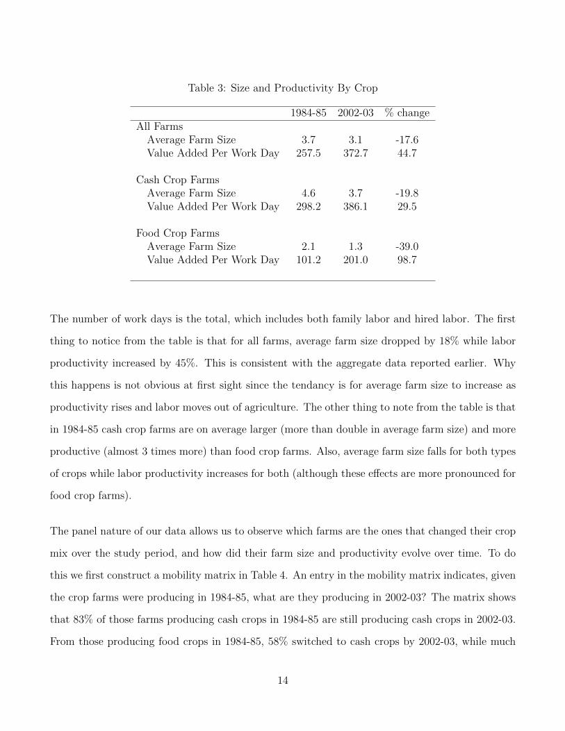
Table 3: Size and Productivity By Crop

1984-85 2002-03 % changeAll Farms

Average Farm Size 3.7 3.1 -17.6Value Added Per Work Day 257.5 372.7 44.7

Cash Crop FarmsAverage Farm Size 4.6 3.7 -19.8Value Added Per Work Day 298.2 386.1 29.5

Food Crop FarmsAverage Farm Size 2.1 1.3 -39.0Value Added Per Work Day 101.2 201.0 98.7

The number of work days is the total, which includes both family labor and hired labor. The first

thing to notice from the table is that for all farms, average farm size dropped by 18% while labor

productivity increased by 45%. This is consistent with the aggregate data reported earlier. Why

this happens is not obvious at first sight since the tendancy is for average farm size to increase as

productivity rises and labor moves out of agriculture. The other thing to note from the table is that

in 1984-85 cash crop farms are on average larger (more than double in average farm size) and more

productive (almost 3 times more) than food crop farms. Also, average farm size falls for both types

of crops while labor productivity increases for both (although these effects are more pronounced for

food crop farms).

The panel nature of our data allows us to observe which farms are the ones that changed their crop

mix over the study period, and how did their farm size and productivity evolve over time. To do

this we first construct a mobility matrix in Table 4. An entry in the mobility matrix indicates, given

the crop farms were producing in 1984-85, what are they producing in 2002-03? The matrix shows

that 83% of those farms producing cash crops in 1984-85 are still producing cash crops in 2002-03.

From those producing food crops in 1984-85, 58% switched to cash crops by 2002-03, while much

14

Table 4: Crop Mobility Matrix

2002-031984-85 cash crops food crops

cash crops 0.83 0.17

food crops 0.58 0.42

Table 5: Mobility Matrix - Size

2002-031984-85 cash cr. food cr.

cash cr. 5.1 2.3

food cr. 2.5 1.6

AFS, 1984-85

2002-031984-85 cash cr. food cr.

cash cr. -16.5 -68.3

food cr. -5.6 1.3

AFS, % change

less switching occurred the other way. So overall there was a shift of farmers towards cash cropping

(as was seen with the summary statistics earlier).

In Tables 5 and 6 we examine what the levels and the changes in average farm size and productivity

respectively, for each of the four entries in the crop mobility matrix. Of particular interest, are the

characteristics of the farms that switched from food crops to cash crops. The tables indicate that,

from the food crop farms in 1984-85, it was the largest in size and the most productive among food

crop farms that switched to cash cropping by 2002-03. Also these switching farms are the ones that

exhibited the strongest productivity growth among all farms over the time period (largely the effect

of catch-up within the cash crop).

15

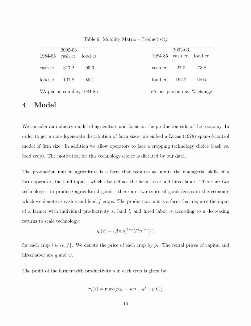
Table 6: Mobility Matrix - Productivity

2002-031984-85 cash cr. food cr.

cash cr. 317.2 95.6

food cr. 107.8 85.1

VA per person day, 1984-85

2002-031984-85 cash cr. food cr.

cash cr. 27.0 78.8

food cr. 162.2 150.5

VA per person day, % change

4 Model

We consider an industry model of agriculture and focus on the production side of the economy. In

order to get a non-degenerate distribution of farm sizes, we embed a Lucas (1978) span-of-control

model of firm size. In addition we allow operators to face a cropping technology choice (cash vs.

food crop). The motivation for this technology choice is dictated by our data.

The production unit in agriculture is a farm that requires as inputs the managerial skills of a

farm operator, the land input - which also defines the farm’s size and hired labor. There are two

technologies to produce agricultural goods: there are two types of goods/crops in the economy

which we denote as cash c and food f crops. The production unit is a farm that requires the input

of a farmer with individual productivity s, land l, and hired labor n according to a decreasing

returns to scale technology:

yi(s) = (Aκis)1−γ(lαn1−α)γ,

for each crop i ∈ {c, f}. We denote the price of each crop by pi. The rental prices of capital and

hired labor are q and w.

The profit of the farmer with productivity s in each crop is given by

πi(s) = max{piyi − wn− ql − piCi}

16

where Ci is a fixed cost of operation in each crop in units of output of the crop. The first order

conditions with respect to land and hired labor inputs are given by eqns 2 and 3 in notes. We note

that these FOC’simply:

n

l=

(1− α)

α

q

w,

It is optimal for farmers in both crops to choose the same hired labor - land ratio regardless of size.

The input demand functions are the following:

li(s) =

(α

q

) 1−γ(1−α)1−γ

(1− αw

) γ(1−α)1−γ

(γpi)1

1−γAκis,

li(s) =

(α

q

) γα1−γ(

1− αw

) 1−γα1−γ

(γpi)1

1−γAκis,

Given these demands, yi(s) can be readily computed. Profits can be written as:

πi(s) = (1− γ)piyi(s)− piCi.

Note that the input demand functions are linear in s and so is output. Then profits is an affine

function of s. We can derive the optimal functions n, l, y, pi which are all afine functions of s. Thus,

more able farmers operate larger farms, demand more labor, produce more output, and make more

profits. Then for a given distribution of managerial ability the model implies a distribution of farm

sizes.

The productivity of farmers is drown from a discrete set S according to a cdf F (s) and pdf f(s).

Given that πi(s) is affine in s, there are two thresholds that determine the fraction of people being

workers, cash crop farmers and food crop farmers. We denote the occupational choice by oi(s) with

the convention that oi(s) = 1 if πi ≥ max{π−i(s), w} so an individual with ability s chooses to

17

operate a farm in crop i and 0 otherwise. Then the clearing conditions are:

∑i

∑s

li(s)oi(s)f(s) = L,

∑i

∑s

ni(s)oi(s)f(s) = Nw

where Nw =∑

i

∑s(1− oi(s))f(s) is the fraction of workers in the economy.

A competitive equilibrium is a set of prices (q, w), occupational decision rules oi(s), and farmers

decision functions ni(s), li(s), πi(s) such that: (i) Given prices, farmers optimize, (ii) Given prices,

oi are optimal occupational choice decisions, and (iii) markets clear.

For reasonable parameter values that are in line with the calibration (κc > κf and Cc > Cf ) the

occupational choice and crop choice decisions of farmers are characterized by two thresholds s and

s, such that,

πf (s) = w

πf (s) = πc(s)

Then those farmers with ability below s will become hired workers, those with ability between

s and s will become food farm operators, and those with ability above s will become cash crop

operators. So s determines the split between operators and farmers (occupational choice decision)

and s determines the split between cash croppers and food croppers (crop technology choice).

4.1 Land Reform

We model land reform as a maximum land level lmax ceiling for farm size. In general, farm operation

cannot exceed this level although in practice there are a few farms that do. This occurs mainly

18

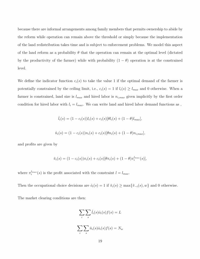
because there are informal arrangements among family members that permits ownership to abide by

the reform while operation can remain above the threshold or simply because the implementation

of the land redistribution takes time and is subject to enforcement problems. We model this aspect

of the land reform as a probability θ that the operation can remain at the optimal level (dictated

by the productivity of the farmer) while with probability (1 − θ) operation is at the constrained

level.

We define the indicator function ci(s) to take the value 1 if the optimal demand of the farmer is

potentially constrained by the ceiling limit, i.e., ci(s) = 1 if li(s) ≥ lmax and 0 otherwise. When a

farmer is constrained, land size is lmax and hired labor is ni,max given implicitly by the first order

condition for hired labor with li = lmax. We can write land and hired labor demand functions as ,

li(s) = (1− ci(s))li(s) + ci(s)[θli(s) + (1− θ)lmax],

ni(s) = (1− ci(s))ni(s) + ci(s)[θni(s) + (1− θ)ni,max],

and profits are given by

πi(s) = (1− ci(s))πi(s) + ci(s)[θπi(s) + (1− θ)πlmaxi (s)],

where πlmaxi (s) is the profit associated with the constraint l = lmax.

Then the occupational choice decisions are oi(s) = 1 if πi(s) ≥ max{π−i(s), w} and 0 otherwise.

The market clearing conditions are then:

∑i

∑s

li(s)oi(s)f(s) = L

∑i

∑s

ni(s)oi(s)f(s) = Nw

19

where Nw is the share of hired labor in the economy, i.e.,Nw =∑

i

∑s(1− oi(s))f(s).

Hence, land reform affects not only land demand directly, but indirectly affect hired labor, occu-

pational choice decisions and demand functions of unconstrained farmers by general equilibrium

effects.

5 Quantitative Analysis

5.1 Calibration

We calibrate a benchmark economy without any restriction on farm size to pre-reform Philip-

pines, using the survey data. The parameters to be calibrated are: technological parameters

{A, κc, κf , α, γ, {s}}, distributional parameters, and the land endowment L. Some parameter values

are chosen based on a priori information, while others are solved for as part of the solution to the

model’s equilibrium in order to match targets in the data.

We choose the distribution of farmer ability to match the distribution of farm sizes in the survey data

(panel) in 1984-85. The distribution of farmer ability is approximated by a log-normal distribution

with mean µ and variance σ2. We approximate the set of farmer abilities with a linearly spaced grid

of 6000 points in [smin, smax], with smin close to 0 and smax equal to 15 which ensures a maximum

sized farm of 23 hectares, the largest farm in our panel in 1984-85. Our calibration involves a loop

for the parameters of the productivity distribution: given values for (µ, σ), we construct a discrete

approximation to a log-normal distribution of ability and solve the model matching the rest of the

targets. The model then yields a distribution of farm sizes. We choose (µ, σ) to minimize the

distance between the size distribution of farms in the model relative to the data.

20

We normalize economy-wide productivity A and the food crop-specific productivity κf to 1 for the

benchmark economy. Given that the two crop prices are exogenous in our formulation we normalize

the relative price of cash crops to food crops to unity. We set the span-of-control parameter to

0.7 and then choose α to match a land income share of 20%. The aggregate land endowment is

chosen to match an average farm size of 3.7 hectares (panel data for 1984-85). We then choose the

remaining parameters - the two fixed operating costs (Cf , Cc) and the cash crop TFP κc - to match

three data targets: (1) a share of hired labor in total farm labor of 61.1%; (2) a share of cash crop

operators in total operators of 61.7%; (3) a ratio of average output per worker between cash crops

and food crops of 2.95. The model parameters along with their targets and calibrated values are

provided in Table 7.

Table 7: Parameterization

Parameter Value Target

Technological ParametersA 1 Normalizationκf 1 Normalizationpc/pf 1 Normalizationγ 0.7 span-of-controlα 0.3 land income shareκc 1.21 Ratio of average crop productivitiesCf -0.56751 Share of hired labor in total farm laborCc -0.51119 Share of cash crop operators in total operators

Parameters of Ability Distributionµ -0.85714 Size distributionσ 1.25 Size distribution

Land EndowmentL 1.4393 Average farm size

The calibrated model does well in matching the farm size distribution by choice of the parameters

of the ability distribution (see Figure 4). While not calibrated to do so the model matches well the

distribution of land, e.g. it reproduces the observation that about 45% of the land is in farms of

less than 5 ha (see Figure 5).

21

<1 1−2 2−5 5−7 7−10 10−15 15+0

0.05

0.1

0.15

0.2

0.25

0.3

0.35

Farm Size Class in Ha

Fra

ction o

f F

arm

s

Model

Data

Figure 4: Share of Farms by Size

<1 1−2 2−5 5−7 7−10 10−15 15+0

0.05

0.1

0.15

0.2

0.25

0.3

0.35

Farm Size Class in Ha

Fra

ction o

f Land

Model

Data

Figure 5: Share of Land in Farms by Size

22

Table 8: Changes in Farm Size and Productivity

Enforcementθ = 1 θ = 0.5 θ = 0.2 θ = 0

Average Farm Size (%∆) 0 -3.6 -6.6 -9.3

Output Per Worker (%∆) 0 -1.9 -3.5 -5.0

5.2 Results

The main quantitative experiment we conduct is the following: we take the benchmark economy

calibrated to pre-reform Philippines, and consider the land reform variant of the model of Section

4.1, feeding in the legislated ceiling of 5 hectares. In Table 8 we show the effect of the land reform

on farm size and productivity for different levels of enforcement θ. The results indicate that the

land reform leads to a drop in both labor productivity and average farm size. Further, the drops

in productivity and average farm size are larger the greater the degree of enforcement (lower θ). A

value of θ = 1 means that the reform is not enforced at all, so there is no change in average farm

size or productivity. A value of θ = 0 means that the land reform is fully enforced so the effects are

the strongest: a 5% drop in productivity and a 9.3% drop in average farm size. In the data 16%

of farms are more than 5 hectares. The θ that guarantees this share is around 0.01 (closer to 0 in

other words).

Next, we study in more detail what causes the drop in productivity in the model by examining

the effect of the reform on productivity growth by crop and the occupational choice allocation. We

focus on the case of full enforcement of the land reform. The results are presented in Table 9.

The intuition behind the main mechanism of the model is the following. The land reform by

imposing a ceiling on land holdings reduces the farm size for all farmers s that had a farm operation

23

Table 9: Effects of Land Reform (θ = 0)

%∆ in aggregate output per worker -5.0

%∆ in cash crop output per worker -6.9

%∆ in food crop output per worker 3.3

∆ in hired labor (%) - 1.0

∆ in cash crop operators (%) 5.0

∆ in food crop operators (%) -4.0

above the ceiling (direct effect) - these are the constrained farmers. This causes an oversupply of

land in the land market reducing the price of land q. For a given occupational allocation between

hired workers - operators and food crop operators - cash crop operators, the decline in farm size for

the constrained operators implies a decline in the demand for labor for the constrained operators,

given the hired labor is proportional to farm size. This tends to reduce the overall demand for labor

in the market, which tends to reduce the wage rate w.

The decrease in the wage rate and the rental price of land means that factor inputs are now

cheaper, which increases the demand for hired labor and land by the unconstrained operators

(general equilibrium effect). The misallocation effect of the land reform on productivity is the

reallocation of farming activity from larger more productive operators to smaller less productive

operators. In other words, the land reform distorts size by inefficiently “propping up” previously

small farms and restricting efficient large farms - so that less able operators become artificially

large. This reduces both farm size and productivity. For a given allocation of hired workers-

operators (i.e., given s) the decrease in w and q increase the profits for all food crop farmers (see

profits in equilibrium) while reducing w. This means that there will be an increase in the number

of operators and a decrease in the number of hired workers. In other words, as s falls some farmers

24

switch from hired workers to operators. Note, that the generated increase in the demand for hired

labor tends to increase w.

For a given allocation of food crop operators - cash crop operators (i.e. for a given s) and for given

decreases in w, q profits will increase for both food crop farmers and cash crop farmers but will

increase more so for cash crop farmers because κc > κf . That is, there is a switch of operators to

the higher productivity crop, so you get more operators flowing to cash crops. These changes in the

occupational allocation and crop choice of farmers impart a selection effect on productivity. The

decrease in s means that you get more low ability operators in food crops. The decrease in s means

that the more able food crop farmers are switching to cash crops. These effects will both tend to

dampen productivity in food crops. But these food crop farmers are the ones that are less likely to

be constrained. So because of the general equilibrium effect of the decrease in w and q they hire

more and produce more. Here this positive productivity effect dominates the effect of the selection

effect and food crop farming productivity increases in equilibrium. The decline in s means that

you have more low ability operators entering cash cropping. This selection effect tends to dampen

productivity. Plus, these operators are the ones being hit by the ceiling. Combined these effects

reduce productivity in cash crops. The overall effect on selection depends on these changes as well

as output shares (plus some other minor terms). Given that cash crops have the highest output

share, quantitatively the selection in cash cropping dominates leading to a fall in productivity. So

here both the selection and reallocation effects reduce productivity. However, selection could in

principle go the other way if the food crops’ effect dominated (i.e., if they had the higher output

share).

We also decompose the overall effect on productivity into the reallocation and misallocation effects.

The counterfactual experiment we run is the following: what would be the effect on productivity if

we precluded the occupational allocation to change but still required the land and labor markets to

clear - that is, if reallocation was the only channel through which productivity was changing. The

25

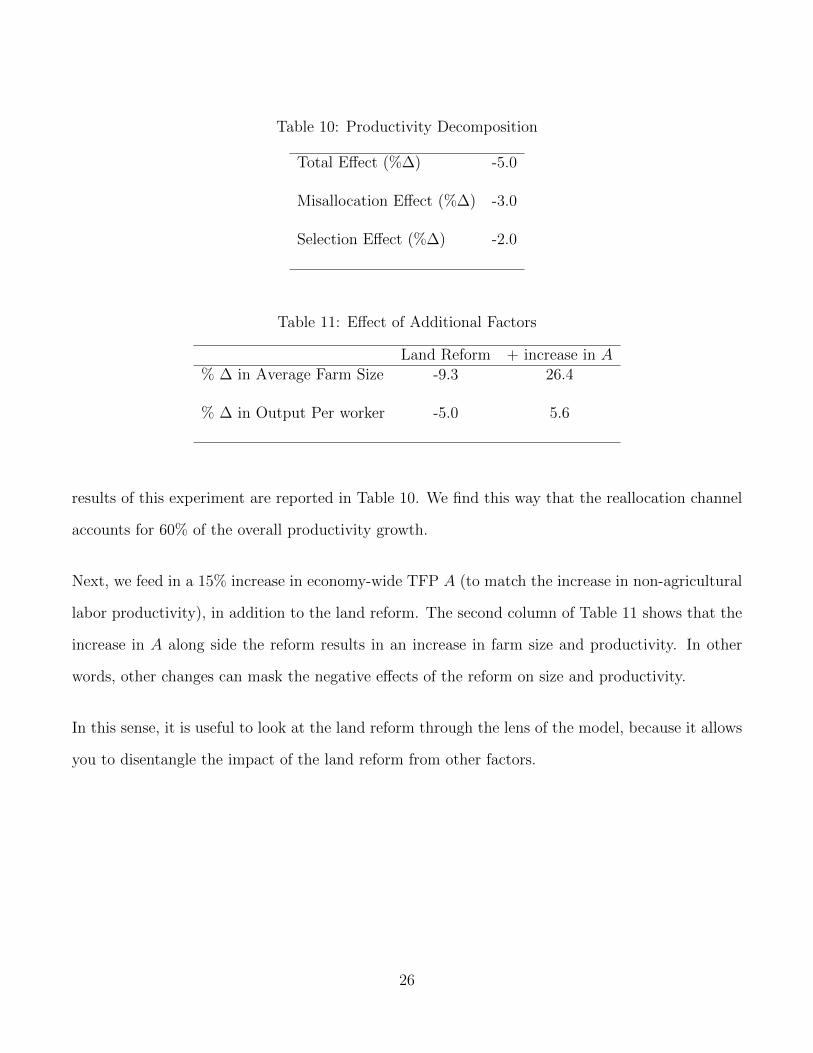
Table 10: Productivity Decomposition

Total Effect (%∆) -5.0

Misallocation Effect (%∆) -3.0

Selection Effect (%∆) -2.0

Table 11: Effect of Additional Factors

Land Reform + increase in A% ∆ in Average Farm Size -9.3 26.4

% ∆ in Output Per worker -5.0 5.6

results of this experiment are reported in Table 10. We find this way that the reallocation channel

accounts for 60% of the overall productivity growth.

Next, we feed in a 15% increase in economy-wide TFP A (to match the increase in non-agricultural

labor productivity), in addition to the land reform. The second column of Table 11 shows that the

increase in A along side the reform results in an increase in farm size and productivity. In other

words, other changes can mask the negative effects of the reform on size and productivity.

In this sense, it is useful to look at the land reform through the lens of the model, because it allows

you to disentangle the impact of the land reform from other factors.

26

References

Adamopoulos, T., and D. Restuccia (forthcoming), “The Size Distribution of Farms and Interna-

tional Productivity Differences,” American Economic Review.

Banerjee, A. V. (1999), “Prospects and Strategies for Land Reforms,” in B. Pleskovic and J. Stiglitz

(eds), Annual World Bank Conference on Development Economics 1999, Washington, DC, World

Bank, 253-84.

Besley, T., and R. Burgess (2000),“Land Reform, Poverty Reduction, and Growth: Evidence from

India,” Quarterly Journal of Economics, 389-430.

Borras, S.M. (2003), “Inclusion-Exclusion in Public Policies and Policy Analyses: The Case of

Philippine Land Reform, 1972-2002,” Journal of International Development 15, 1049-1065.

Bouis, H.E., and L.J. Haddad (1990), Agricultural Commercialization, Nutrition, and the Rural

Poor: A Study of Philippine Farm Households, Boulder, Colorado, U.S.A: Lynne Rienner.

Lucas, R. (1978), “On the Size Distribution of Business Firms,” Bell Journal of Economics, 9(2),

508-23.

Restuccia, D., D.T. Yang, and X. Zhu (2008), “Agriculture and Aggregate Productivity: A Quan-

titative Cross-Country Analysis”, Journal of Monetary Economics 55(2), 234-250.

Saulo-Adriano, L. (1991), “A General Assessment of the Comprehensive Agrarian Reform Program,”

Working Paper Series No.91-13, Philippine Institute for Development Studies.

27