Landmark-Based Speech Recognition:

Report of the 2004 Johns Hopkins Summer Workshop

Mark Hasegawa-Johnson (jhasegaw@uiuc.edu),James Baker (jim@sandboxscribe.com),

Steven Greenberg (steveng@cogsci.berkeley.edu),Katrin Kirchhoff (katrin@ee.washington.edu),Jennifer Muller (jsmuller@ling.ohio-state.edu),

Kemal Sonmez (kemal@speech.sri.com),Sarah Borys (sborys@uiuc.edu),Ken Chen (kenchen@ucsd.edu),

Amit Juneja (juneja@glue.umd.edu),Karen Livescu (klivescu@sls.csail.mit.edu),

Srividya Mohan (srividya@jhu.edu),Emily Coogan (ecoogan@uiuc.edu),

Tianyu Wang (gtg746b@prism.gatech.edu)1

January 31, 2005

1This research would have been impossible without the support of Andreas Stolcke, John Makhoul, OwenKimball, Spyros Matsoukas, Dimitra Vergyri, Luciana Ferrer, Nima Mesgarani, Yanli Zheng, Tarun Pruthi,Shihab Shamma, Carol Espy-Wilson, Jeff Bilmes, Partha Niyogi, Jim Glass, T.J. Hazen, Eric Fosler-Lussier,Fred Jelinek, Sanjeev Khudanpur, the National Science Foundation, and the Department of Defense.

Contents

1 Introduction 3

1.1 Methods: Overview . . . . . . . . . . . . . . . . . . . . . . . . . . . . . . . . . . . . . 4

2 Background 6

2.1 Speech Perception: Distinctive Features . . . . . . . . . . . . . . . . . . . . . . . . . 62.2 Speech Perception: Landmarks . . . . . . . . . . . . . . . . . . . . . . . . . . . . . . 92.3 Pronunciation Variability . . . . . . . . . . . . . . . . . . . . . . . . . . . . . . . . . 122.4 Empirical Study of Pronunciation Variability . . . . . . . . . . . . . . . . . . . . . . 14

3 Distinctive Feature Definition 17

3.1 Distinctive Features . . . . . . . . . . . . . . . . . . . . . . . . . . . . . . . . . . . . 173.1.1 Manner of Articulation . . . . . . . . . . . . . . . . . . . . . . . . . . . . . . 213.1.2 Syllable Structure . . . . . . . . . . . . . . . . . . . . . . . . . . . . . . . . . 233.1.3 Voicing . . . . . . . . . . . . . . . . . . . . . . . . . . . . . . . . . . . . . . . 233.1.4 Place of Articulation . . . . . . . . . . . . . . . . . . . . . . . . . . . . . . . . 243.1.5 Vowel Features . . . . . . . . . . . . . . . . . . . . . . . . . . . . . . . . . . . 25

3.2 Entropes . . . . . . . . . . . . . . . . . . . . . . . . . . . . . . . . . . . . . . . . . . . 253.2.1 The Significance of Entropy for Lexical Discrimination . . . . . . . . . . . . . 263.2.2 What is an Entrope? . . . . . . . . . . . . . . . . . . . . . . . . . . . . . . . . 263.2.3 The Importance of Prosodic Accent . . . . . . . . . . . . . . . . . . . . . . . 293.2.4 Computation of Entropic Potential . . . . . . . . . . . . . . . . . . . . . . . . 293.2.5 The Boundary Valence - Binding Syllables . . . . . . . . . . . . . . . . . . . . 303.2.6 Entropy Hierarchy . . . . . . . . . . . . . . . . . . . . . . . . . . . . . . . . . 303.2.7 Automatic Generation of Pronunciation Models . . . . . . . . . . . . . . . . . 31

4 Landmark Detection and Classification 32

4.1 Related Work . . . . . . . . . . . . . . . . . . . . . . . . . . . . . . . . . . . . . . . . 324.2 Speech Data and Acoustic Observations . . . . . . . . . . . . . . . . . . . . . . . . . 344.3 SVM Computation of Posterior Probabilities . . . . . . . . . . . . . . . . . . . . . . 354.4 Frame-Based Manner Classification . . . . . . . . . . . . . . . . . . . . . . . . . . . . 354.5 Landmark Detection SVMs . . . . . . . . . . . . . . . . . . . . . . . . . . . . . . . . 374.6 Place Classification Results . . . . . . . . . . . . . . . . . . . . . . . . . . . . . . . . 394.7 Vowel Nasalization . . . . . . . . . . . . . . . . . . . . . . . . . . . . . . . . . . . . . 424.8 Prosody . . . . . . . . . . . . . . . . . . . . . . . . . . . . . . . . . . . . . . . . . . . 444.9 Use of Duration Probabilities to Improve Landmark Detection Accuracy . . . . . . . 474.10 Discussion . . . . . . . . . . . . . . . . . . . . . . . . . . . . . . . . . . . . . . . . . . 48

1

5 Rescoring Using a Generative Feature-Based Pronunciation Model 51

5.1 From Words to Landmarks and Distinctive Features . . . . . . . . . . . . . . . . . . 525.1.1 The Production-Based Pronunciation Model . . . . . . . . . . . . . . . . . . . 525.1.2 Integration with SVM classifiers . . . . . . . . . . . . . . . . . . . . . . . . . 54

5.2 Related Work . . . . . . . . . . . . . . . . . . . . . . . . . . . . . . . . . . . . . . . . 565.3 Experiments . . . . . . . . . . . . . . . . . . . . . . . . . . . . . . . . . . . . . . . . . 575.4 Discussion . . . . . . . . . . . . . . . . . . . . . . . . . . . . . . . . . . . . . . . . . . 59

6 Discriminative Rescoring Using Landmarks 63

6.1 Conversion to Confusion Networks . . . . . . . . . . . . . . . . . . . . . . . . . . . . 636.2 Landmark Selection Using a Maximum-Entropy Technique . . . . . . . . . . . . . . . 656.3 Score Queries and Rescoring . . . . . . . . . . . . . . . . . . . . . . . . . . . . . . . . 666.4 Results and Analysis . . . . . . . . . . . . . . . . . . . . . . . . . . . . . . . . . . . . 676.5 Conclusions . . . . . . . . . . . . . . . . . . . . . . . . . . . . . . . . . . . . . . . . . 68

7 Lattice Rescoring 69

7.1 Introduction . . . . . . . . . . . . . . . . . . . . . . . . . . . . . . . . . . . . . . . . . 697.2 Existing Approaches . . . . . . . . . . . . . . . . . . . . . . . . . . . . . . . . . . . . 697.3 Maximum Entropy WER-based Rescoring of Confusion Networks . . . . . . . . . . . 707.4 Features and Experiments . . . . . . . . . . . . . . . . . . . . . . . . . . . . . . . . . 71

8 Conclusions 73

A Appendices 74

A.1 Support Vector Machine Tutorial . . . . . . . . . . . . . . . . . . . . . . . . . . . . . 74A.2 Articulatory Feature Set . . . . . . . . . . . . . . . . . . . . . . . . . . . . . . . . . . 76A.3 Phoneme-to-AF and AF-to-DF Mappings . . . . . . . . . . . . . . . . . . . . . . . . 76

2

Chapter 1

Introduction

The goal of the Landmark-Based Speech Recognition team at WS04 was to develop a radically newclass of speech recognition acoustic models by (1) using regularized machine learning algorithms inhigh-dimensional observation spaces to train the parameters of (2) psychologically realistic informa-tion structures. Six faculty-level researchers, four graduate students, and two undergraduates spentsix weeks at Johns Hopkins University (July 4-August 16, 2004) training and testing technologicalmodels of the acoustic and pronunciation variability of words in conversational telephone speech.None of the tested systems was able to beat the state of the art for conversational telephone speech,but a number of subsidiary goals were successfully achieved, and these successes indicate a pathforward for this research. Specific successes include the following. First, support vector machines(SVMs) were able to perform many binary phoneme detection and classification tasks with verylow error rates; for example, CV and VC transitions (onsets and offsets of the feature [consonan-tal]) were detected with 3% per-frame error rate, on a task for which chance is 50%. Second, adynamic Bayesian network (DBN) pronunciation model, coupled with SVM phonetic classifiers, wasable to correctly label the articulatory changes underlying radical pronunciation variants including/n/→nasalized vowel, /t/→alveolar glide, /g/→/y/. Third, a rescoring system was able to success-fully choose salient landmark differences among the words in alternate recognizer hypotheses, and tocall landmark detectors as necessary to choose the better hypothesis. Preliminary error analysis sug-gests that, with training data more fully representative of pronunciation variants in conversationaltelephone speech, the rescoring system would have achieved a statistically significant improvementin word error rate.

Since at least 1955, psychophysical experiments in human speech perception have demonstratedthat speech perception is multi-scale and structured: coarse-scale information (prosody, syllablestructure, sonorancy) can be perceived independently of fine-grained information (place of articula-tion) [118, 146, 116, 89, 90, 142, 20, 52]. Human ability to generalize quickly and effortlessly fromone speaking style, signal-to-noise ratio (SNR), or channel condition to another has been attributedto this multi-scale characteristic of speech perception [1, 76, 144]. Despite the importance of multi-scale perception in human speech perception, psychologically realistic multi-scale models have failedto outperform single-scale models such as the hidden Markov model (HMM). The apparent causeof the success of the HMM is the property of simultaneously optimal parameters: it is possible tosimultaneously adjust every parameter in an HMM in order to optimize a global recognition per-formance metric (maximum likelihood, maximum mutual information, or minimum classificationerror). Until the 1990s, the HMM was the only large vocabulary speech recognition model withthe characteristic of simultaneously optimal parameters and, therefore, psychologically realistic hi-erarchical multi-scale models were not competitive. The research performed at WS04 demonstrates,we believe, that the HMM is no longer the only game in town. We have developed psychologicallyrealistic multi-scale speech recognition models with parameters that can be optimized in pursuit of

3

a global speech recognition performance metric.Current-generation automatic speech recognition (ASR) systems are based on an architecture

(HMMs) that is both time-consuming to train, and extremely vulnerable to acoustic interference andvariation in speaking style. The conventional methods for enhancing ASR performance often requireenormous amounts of data collection and annotation, as well as extensive training on representativematerial. This dependence on training materials shapes the entire fabric of ASR methodologyand makes it exceedingly difficult (and expensive) to introduce innovative concepts into speechrecognition. As a consequence, the pace of innovation and refinement is considerably slower than itmight otherwise be.

Current-generation ASR systems represent words as sequences of context-dependent phonemes.In order to train acoustic models proficient in classifying phonemic units vast amounts of trainingmaterial are required. Even with such material, state-of-the-art recognition systems generally mis-classify 30 to 40% of the phonetic constituents [62]. Performance improves only slightly when a wordtranscript is provided. And yet, phonetic classification is critical for ASR performance; the worderror rate (WER) is highly correlated with phonetic classification error [64, 65]. Substantial improve-ment of phonetic classification would likely yield a significant gain in ASR performance. Moreover,if phonetic classification were extremely accurate, and pronunciation models in the lexicon preciselymatched the phonetic classification data, ASR performance would improve dramatically [114]. Un-fortunately, ASR systems are nowhere close to achieving such goals. An entirely different approachis required - one that melds state-of-the-art phonetic classifiers with realistic pronunciation modelsrepresentative of the speaking styles and conditions associated with the recognition task.

1.1 Methods: Overview

This report describes both phoneme classification and large vocabulary speech recognition systemsthat use a landmark-based, distinctive-feature based lexical representation. The goal of all researchdescribed in this report is as follows: we aim to apply recently developed methods from artificialintelligence (specifically support vector machines, dynamic Bayesian networks, and maximum en-tropy classification) in order to implement, in the form of an automatic speech recognizer, currenttheories of human speech perception and phonology (specifically landmark-based speech perception,nonlinear phonology, and articulatory phonology).

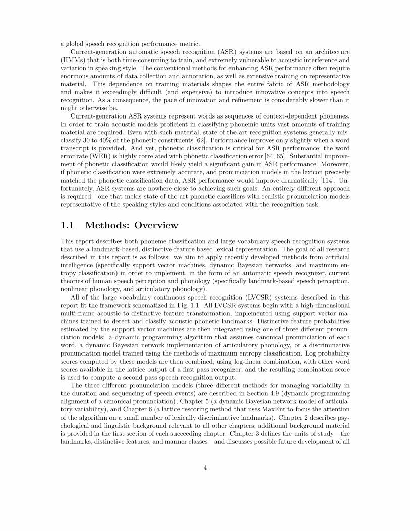
All of the large-vocabulary continuous speech recognition (LVCSR) systems described in thisreport fit the framework schematized in Fig. 1.1. All LVCSR systems begin with a high-dimensionalmulti-frame acoustic-to-distinctive feature transformation, implemented using support vector ma-chines trained to detect and classify acoustic phonetic landmarks. Distinctive feature probabilitiesestimated by the support vector machines are then integrated using one of three different pronun-ciation models: a dynamic programming algorithm that assumes canonical pronunciation of eachword, a dynamic Bayesian network implementation of articulatory phonology, or a discriminativepronunciation model trained using the methods of maximum entropy classification. Log probabilityscores computed by these models are then combined, using log-linear combination, with other wordscores available in the lattice output of a first-pass recognizer, and the resulting combination scoreis used to compute a second-pass speech recognition output.

The three different pronunciation models (three different methods for managing variability inthe duration and sequencing of speech events) are described in Section 4.9 (dynamic programmingalignment of a canonical pronunciation), Chapter 5 (a dynamic Bayesian network model of articula-tory variability), and Chapter 6 (a lattice rescoring method that uses MaxEnt to focus the attentionof the algorithm on a small number of lexically discriminative landmarks). Chapter 2 describes psy-chological and linguistic background relevant to all other chapters; additional background materialis provided in the first section of each succeeding chapter. Chapter 3 defines the units of study—thelandmarks, distinctive features, and manner classes—and discusses possible future development of all

4

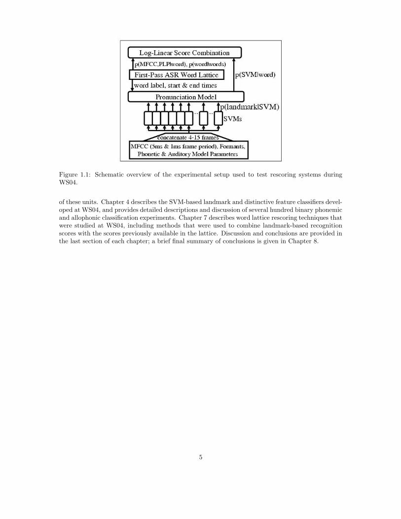
Figure 1.1: Schematic overview of the experimental setup used to test rescoring systems duringWS04.

of these units. Chapter 4 describes the SVM-based landmark and distinctive feature classifiers devel-oped at WS04, and provides detailed descriptions and discussion of several hundred binary phonemicand allophonic classification experiments. Chapter 7 describes word lattice rescoring techniques thatwere studied at WS04, including methods that were used to combine landmark-based recognitionscores with the scores previously available in the lattice. Discussion and conclusions are provided inthe last section of each chapter; a brief final summary of conclusions is given in Chapter 8.

5

Chapter 2

Background

This section reviews some of the background on which the research at WS04 was based. We claim,as the foundation of our research, publications in three disciplines: speech psychology (especiallyspeech perception), linguistics (especially phonology), and machine learning. This section reviewsresults in speech psychology and linguistics; relevant background in machine learning and automaticspeech recognition is reviewed in the first section of each succeeding chapter.

2.1 Speech Perception: Distinctive Features

In 1952, Jakobson, Fant and Halle suggested encoding each phoneme as a vector of binary “distinctivefeatures:” voiced vs. unvoiced, lowpass vs. highpass, spectrally compact vs. spectrally diffuse [82].The idea that a phoneme can be decomposed into independently manipulable dimensions is quite old:classical Greek, Hebrew, Arabic, and Japanese, for example, mark secondary distinctions such asvowel length and consonant gemination (Arabic), voicing (Japanese), and syllable-initial aspirationor glottalization (classical Greek) by means of diacritics. The Hangul writing system, published byKing Sejong of Korea in 1446 [132], independently encodes the place, manner, and voicing of everyconsonant: each consonant is composed of a fundamental symbol encoding place (labial, dental,alveolar, velar, or pharyngeal), modified by diacritics encoding manner and voicing. In 1876, thephonetician Alexander Bell proposed an international phonetic alphabet, capable of representing anyplace or manner distinction specified by any of the world’s languages [8]. Bell’s initial notation wasbased on a symbol encoding the place of the consonant, annotated by diacritics encoding mannerand voicing, much like the Hangul system; because of the high cost of typesetting Bell’s symbols,his notation was eventually replaced by an international consensus system called the InternationalPhonetic Alphabet (IPA) [80]. Given the very long history of place-manner notation, the binarydistinctive feature notation of Jakobson, Fant, and Halle was significant primarily for two reasons.First, their notation was the first to declare that all phonemic distinctions can be encoded in abinary notation, as opposed to the N-ary place and manner distinctions proposed by Sejong andBell. Second, their notation was important in part because, within three years after Jakobson’spaper, Miller and Nicely were able to prove the psychological reality of a nearly binary distinctivefeature notation similar to Jakobson’s [118].

Miller and Nicely [118] asked listeners to transcribe noisy recordings of consonant-vowel syllables.Miller and Nicely compiled their results into confusion matrices, in which element (i, j) of the matrixshows the number of times that phoneme i was mis-recognized as phoneme j (Fig. 2.1). Humanlisteners rarely misunderstand nonsense syllables under quiet listening conditions, but with enoughnoise, it is possible to get listeners to make mistakes, and the mistakes they make are revealing.First, some distinctive features are more susceptible to noise than others: place of articulation isreliably communicated only at SNR above -6dB, while sonorancy is reliably communicated even at

6

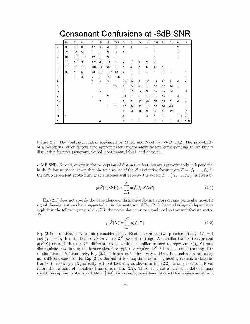
Figure 2.1: The confusion matrix measured by Miller and Nicely at -6dB SNR. The probabilityof a perceptual error factors into approximately independent factors corresponding to six binarydistinctive features (sonorant, voiced, continuant, labial, and alveolar).

-12dB SNR. Second, errors in the perception of distinctive features are approximately independent,in the following sense: given that the true values of the N distinctive features are F = [f1, . . . , fN ]T ,

the SNR-dependent probability that a listener will perceive the vector F = [f1, . . . , fN ]T is given by

p(F |F, SNR) ≈

N∏

i=1

p(fi|fi, SNR) (2.1)

Eq. (2.1) does not specify the dependence of distinctive feature errors on any particular acousticsignal. Several authors have suggested an implementation of Eq. (2.1) that makes signal-dependenceexplicit in the following way, where X is the particular acoustic signal used to transmit feature vectorF :

p(F |X) =

N∏

i=1

p(fi|X) (2.2)

Eq. (2.2) is motivated by training considerations. Each feature has two possible settings (fi = 1and fi = −1), thus the feature vector F has 2N possible settings. A classifier trained to represent

p(F |X) must distinguish 2N different labels, while a classifier trained to represent p(fi|X) onlydistinguishes two labels; the former therefore typically requires 2N−1 times as much training dataas the latter. Unfortunately, Eq. (2.2) is incorrect in three ways. First, it is neither a necessarynor sufficient condition for Eq. (2.1). Second, it is suboptimal as an engineering system: a classifiertrained to model p(F |X) directly, without factoring as shown in Eq. (2.2), usually results in fewererrors than a bank of classifiers trained as in Eq. (2.2). Third, it is not a correct model of humanspeech perception. Volaitis and Miller [164], for example, have demonstrated that a voice onset time

7

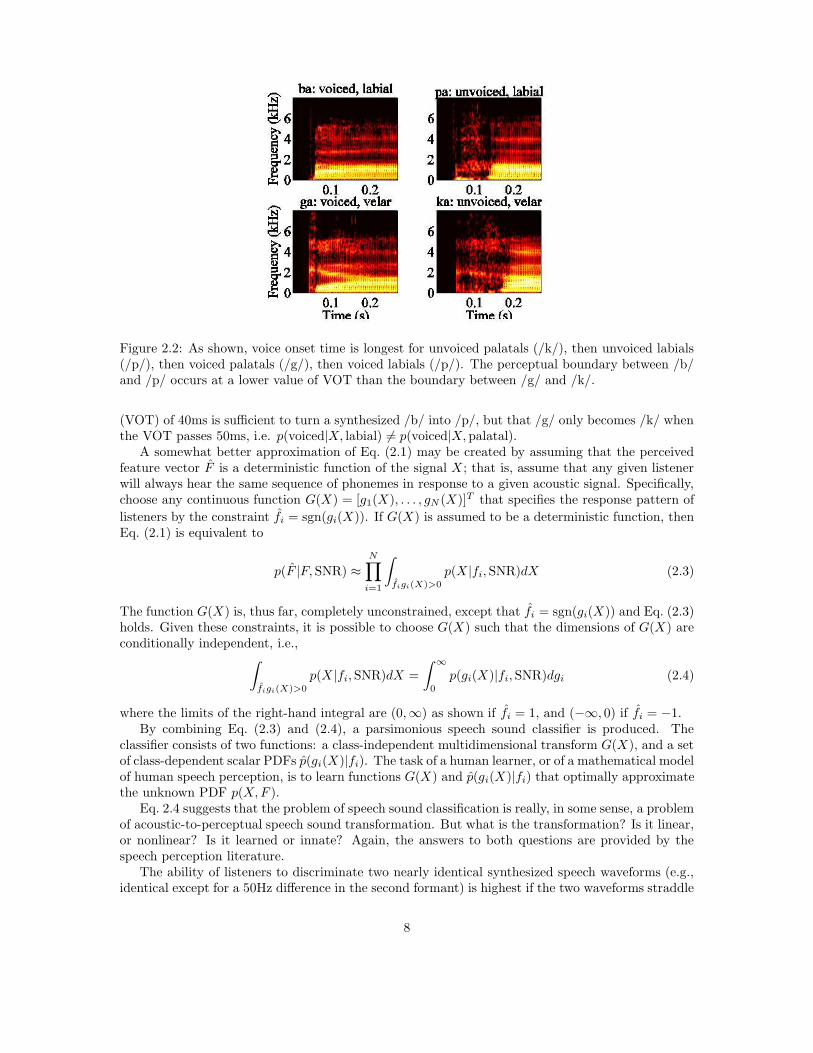
Figure 2.2: As shown, voice onset time is longest for unvoiced palatals (/k/), then unvoiced labials(/p/), then voiced palatals (/g/), then voiced labials (/p/). The perceptual boundary between /b/and /p/ occurs at a lower value of VOT than the boundary between /g/ and /k/.

(VOT) of 40ms is sufficient to turn a synthesized /b/ into /p/, but that /g/ only becomes /k/ whenthe VOT passes 50ms, i.e. p(voiced|X, labial) 6= p(voiced|X, palatal).

A somewhat better approximation of Eq. (2.1) may be created by assuming that the perceivedfeature vector F is a deterministic function of the signal X ; that is, assume that any given listenerwill always hear the same sequence of phonemes in response to a given acoustic signal. Specifically,choose any continuous function G(X) = [g1(X), . . . , gN (X)]T that specifies the response pattern of

listeners by the constraint fi = sgn(gi(X)). If G(X) is assumed to be a deterministic function, thenEq. (2.1) is equivalent to

p(F |F, SNR) ≈

N∏

i=1

∫

figi(X)>0

p(X |fi, SNR)dX (2.3)

The function G(X) is, thus far, completely unconstrained, except that fi = sgn(gi(X)) and Eq. (2.3)holds. Given these constraints, it is possible to choose G(X) such that the dimensions of G(X) areconditionally independent, i.e.,

∫

figi(X)>0

p(X |fi, SNR)dX =

∫ ∞

0

p(gi(X)|fi, SNR)dgi (2.4)

where the limits of the right-hand integral are (0,∞) as shown if fi = 1, and (−∞, 0) if fi = −1.By combining Eq. (2.3) and (2.4), a parsimonious speech sound classifier is produced. The

classifier consists of two functions: a class-independent multidimensional transform G(X), and a setof class-dependent scalar PDFs p(gi(X)|fi). The task of a human learner, or of a mathematical modelof human speech perception, is to learn functions G(X) and p(gi(X)|fi) that optimally approximatethe unknown PDF p(X, F ).

Eq. 2.4 suggests that the problem of speech sound classification is really, in some sense, a problemof acoustic-to-perceptual speech sound transformation. But what is the transformation? Is it linear,or nonlinear? Is it learned or innate? Again, the answers to both questions are provided by thespeech perception literature.

The ability of listeners to discriminate two nearly identical synthesized speech waveforms (e.g.,identical except for a 50Hz difference in the second formant) is highest if the two waveforms straddle

8

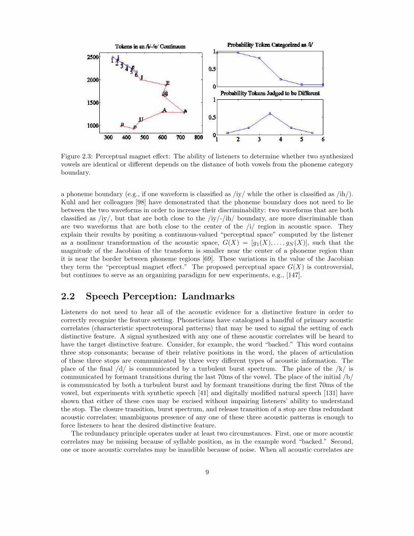
Figure 2.3: Perceptual magnet effect: The ability of listeners to determine whether two synthesizedvowels are identical or different depends on the distance of both vowels from the phoneme categoryboundary.

a phoneme boundary (e.g., if one waveform is classified as /iy/ while the other is classified as /ih/).Kuhl and her colleagues [98] have demonstrated that the phoneme boundary does not need to liebetween the two waveforms in order to increase their discriminability: two waveforms that are bothclassified as /iy/, but that are both close to the /iy/-/ih/ boundary, are more discriminable thanare two waveforms that are both close to the center of the /i/ region in acoustic space. Theyexplain their results by positing a continuous-valued “perceptual space” computed by the listeneras a nonlinear transformation of the acoustic space, G(X) = [g1(X), . . . , gN(X)], such that themagnitude of the Jacobian of the transform is smaller near the center of a phoneme region thanit is near the border between phoneme regions [69]. These variations in the value of the Jacobianthey term the “perceptual magnet effect.” The proposed perceptual space G(X) is controversial,but continues to serve as an organizing paradigm for new experiments, e.g., [147].

2.2 Speech Perception: Landmarks

Listeners do not need to hear all of the acoustic evidence for a distinctive feature in order tocorrectly recognize the feature setting. Phoneticians have catalogued a handful of primary acousticcorrelates (characteristic spectrotemporal patterns) that may be used to signal the setting of eachdistinctive feature. A signal synthesized with any one of these acoustic correlates will be heard tohave the target distinctive feature. Consider, for example, the word “backed.” This word containsthree stop consonants; because of their relative positions in the word, the places of articulationof these three stops are communicated by three very different types of acoustic information. Theplace of the final /d/ is communicated by a turbulent burst spectrum. The place of the /k/ iscommunicated by formant transitions during the last 70ms of the vowel. The place of the initial /b/is communicated by both a turbulent burst and by formant transitions during the first 70ms of thevowel, but experiments with synthetic speech [41] and digitally modified natural speech [131] haveshown that either of these cues may be excised without impairing listeners’ ability to understandthe stop. The closure transition, burst spectrum, and release transition of a stop are thus redundantacoustic correlates; unambiguous presence of any one of these three acoustic patterns is enough toforce listeners to hear the desired distinctive feature.

The redundancy principle operates under at least two circumstances. First, one or more acousticcorrelates may be missing because of syllable position, as in the example word “backed.” Second,one or more acoustic correlates may be inaudible because of noise. When all acoustic correlates are

9

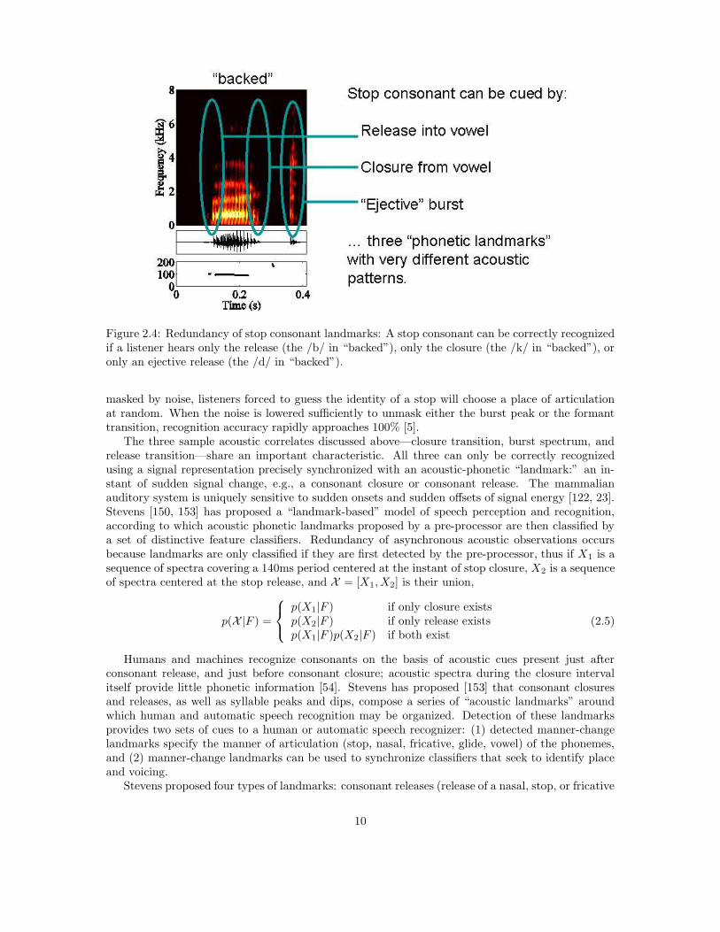
Figure 2.4: Redundancy of stop consonant landmarks: A stop consonant can be correctly recognizedif a listener hears only the release (the /b/ in “backed”), only the closure (the /k/ in “backed”), oronly an ejective release (the /d/ in “backed”).

masked by noise, listeners forced to guess the identity of a stop will choose a place of articulationat random. When the noise is lowered sufficiently to unmask either the burst peak or the formanttransition, recognition accuracy rapidly approaches 100% [5].

The three sample acoustic correlates discussed above—closure transition, burst spectrum, andrelease transition—share an important characteristic. All three can only be correctly recognizedusing a signal representation precisely synchronized with an acoustic-phonetic “landmark:” an in-stant of sudden signal change, e.g., a consonant closure or consonant release. The mammalianauditory system is uniquely sensitive to sudden onsets and sudden offsets of signal energy [122, 23].Stevens [150, 153] has proposed a “landmark-based” model of speech perception and recognition,according to which acoustic phonetic landmarks proposed by a pre-processor are then classified bya set of distinctive feature classifiers. Redundancy of asynchronous acoustic observations occursbecause landmarks are only classified if they are first detected by the pre-processor, thus if X1 is asequence of spectra covering a 140ms period centered at the instant of stop closure, X2 is a sequenceof spectra centered at the stop release, and X = [X1, X2] is their union,

p(X|F ) =

p(X1|F ) if only closure existsp(X2|F ) if only release existsp(X1|F )p(X2|F ) if both exist

(2.5)

Humans and machines recognize consonants on the basis of acoustic cues present just afterconsonant release, and just before consonant closure; acoustic spectra during the closure intervalitself provide little phonetic information [54]. Stevens has proposed [153] that consonant closuresand releases, as well as syllable peaks and dips, compose a series of “acoustic landmarks” aroundwhich human and automatic speech recognition may be organized. Detection of these landmarksprovides two sets of cues to a human or automatic speech recognizer: (1) detected manner-changelandmarks specify the manner of articulation (stop, nasal, fricative, glide, vowel) of the phonemes,and (2) manner-change landmarks can be used to synchronize classifiers that seek to identify placeand voicing.

Stevens proposed four types of landmarks: consonant releases (release of a nasal, stop, or fricative

10

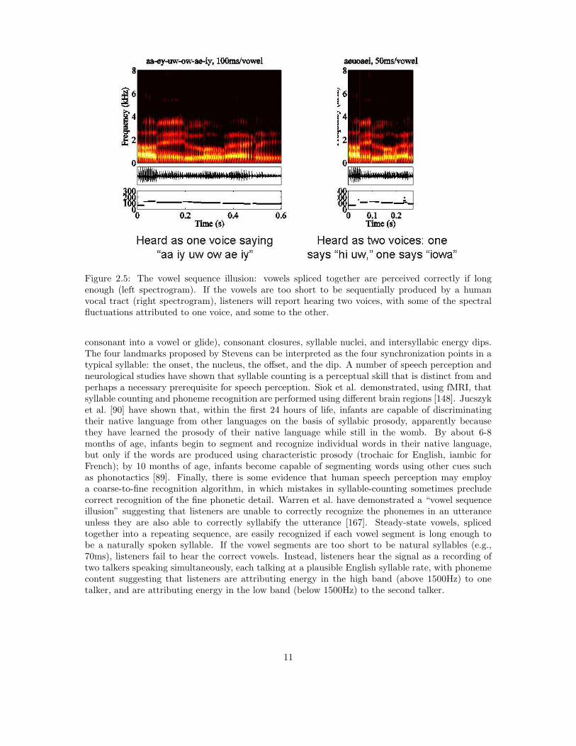
Figure 2.5: The vowel sequence illusion: vowels spliced together are perceived correctly if longenough (left spectrogram). If the vowels are too short to be sequentially produced by a humanvocal tract (right spectrogram), listeners will report hearing two voices, with some of the spectralfluctuations attributed to one voice, and some to the other.

consonant into a vowel or glide), consonant closures, syllable nuclei, and intersyllabic energy dips.The four landmarks proposed by Stevens can be interpreted as the four synchronization points in atypical syllable: the onset, the nucleus, the offset, and the dip. A number of speech perception andneurological studies have shown that syllable counting is a perceptual skill that is distinct from andperhaps a necessary prerequisite for speech perception. Siok et al. demonstrated, using fMRI, thatsyllable counting and phoneme recognition are performed using different brain regions [148]. Jucszyket al. [90] have shown that, within the first 24 hours of life, infants are capable of discriminatingtheir native language from other languages on the basis of syllabic prosody, apparently becausethey have learned the prosody of their native language while still in the womb. By about 6-8months of age, infants begin to segment and recognize individual words in their native language,but only if the words are produced using characteristic prosody (trochaic for English, iambic forFrench); by 10 months of age, infants become capable of segmenting words using other cues suchas phonotactics [89]. Finally, there is some evidence that human speech perception may employa coarse-to-fine recognition algorithm, in which mistakes in syllable-counting sometimes precludecorrect recognition of the fine phonetic detail. Warren et al. have demonstrated a “vowel sequenceillusion” suggesting that listeners are unable to correctly recognize the phonemes in an utteranceunless they are also able to correctly syllabify the utterance [167]. Steady-state vowels, splicedtogether into a repeating sequence, are easily recognized if each vowel segment is long enough tobe a naturally spoken syllable. If the vowel segments are too short to be natural syllables (e.g.,70ms), listeners fail to hear the correct vowels. Instead, listeners hear the signal as a recording oftwo talkers speaking simultaneously, each talking at a plausible English syllable rate, with phonemecontent suggesting that listeners are attributing energy in the high band (above 1500Hz) to onetalker, and are attributing energy in the low band (below 1500Hz) to the second talker.

11

2.3 Pronunciation Variability

Conventional ASR systems model utterances as sequences of words, and words as sequences ofphonemes. As a consequence, pronunciation models contain only phonemic elements. In conversa-tional speech, however, the acoustic implementation of a phoneme varies substantially as a functionof speaking style, dialect, individual idiolect, prosodic context, and phonemic context. Current-generation systems attempt to model variability by creating a variety of context-dependent allophonemodels, including, e.g., triphone and quinphone models, function-word dependent models [101], andmodels dependent on prosodic context variables such as pitch accent and intonational phrase bound-ary [32]. While triphone models are capable of representing a surprising amount of contextual vari-ability, there is a limit to this approach: each 100% increase in the number of trainable allophonemodels requires a 100% increase in the amount of labeled training data. Context-dependent phonemodels have also proven surprisingly incapable of duplicating the high accuracy of human listenersin the task of recognizing phonemes in nonsense syllables. Human listeners recognize phonemesin nonsense syllables with 98.5% accuracy under quiet listening conditions [50, 1, 2]. By contrast,automatic speech recognizers rarely achieve more than 75% phoneme recognition accuracy, even un-der “quiet listening conditions” (e.g., read text). For conversational corpora, such as Switchboard,classification accuracy rarely exceeds 60-70%, even when the words are known in advance (i.e., auto-matic alignments rather than unconstrained recognition is performed) [62]. One may conclude fromsuch evidence that the speech signal is not organized in terms of phonemes, allophones, or any othertemporally sequenced units (“beads on a string”). But which units are more likely to capture thenatural variation observed in spoken language?

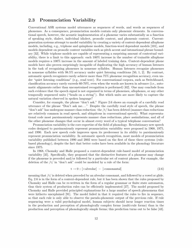
Consider, for example, the phrase “don’t ask.” Figure 2.6 shows an example of a carefully readutterance of the phrase “Don’t ask me. . . ” Despite the carefully read style of speech, the phrase“don’t ask” has undergone manner class reduction: the /t/ has been deleted (manner class reductionsare relatively common in read speech, and ubiquitous in conversational speech). What representa-tional code most parsimoniously represents manner class reductions, place assimilations, and all ofthe other phoneme changes that occur in almost every word of a typical telephone conversation?

Pronunciation variability is the core expertise of the field of phonology. Revolutionary new speechcodes designed to parsimoniously represent pronunciation variability were proposed in 1968, 1975,and 1990. Each new speech code improves upon its predecessor in its ability to parsimoniouslyrepresent pronunciation variability. In automatic speech recognition, most models of pronunciationvariability published between 1990 and 2002 were based on the first of these three systems (rule-based phonology), despite the fact that better codes have been available in the phonology literaturesince 1975.

In 1968, Chomsky and Halle proposed a context-dependent rule-based model of pronunciationvariability [35]. Specifically, they proposed that the distinctive features of a phoneme may changeif the phoneme is preceded and/or followed by a particular set of context phones. For example, thedeletion of the /t/ in “don’t ask” could be modeled by a rule of the form:

t → 0 :: [+alveolar] − [-consonantal] (2.6)

meaning that /t/ is deleted when preceded by an alveolar consonant, and followed by a vowel or glide.Eq. 2.6 is in the form of a context-dependent rule, but it has been shown that the rules proposed byChomsky and Halle can be re-written in the form of a regular grammar or finite state automaton,thus their system of production rules can be efficiently implemented [27]. The model proposed byChomsky and Halle provided principled explanations for a large number of speech phenomena thatwere hitherto unexplained [91]. The model failed in that it required the rules to fire in sequence,so that each rule is only able to observe the pseudo-phonemic output of the previous rule. If rulesequencing were a valid psychological model, human subjects should incur longer reaction timesin the production and perception of phonologically complex forms (multi-rule forms) than in theproduction and perception of phonologically simple forms; this prediction turns out to be false [43].

12

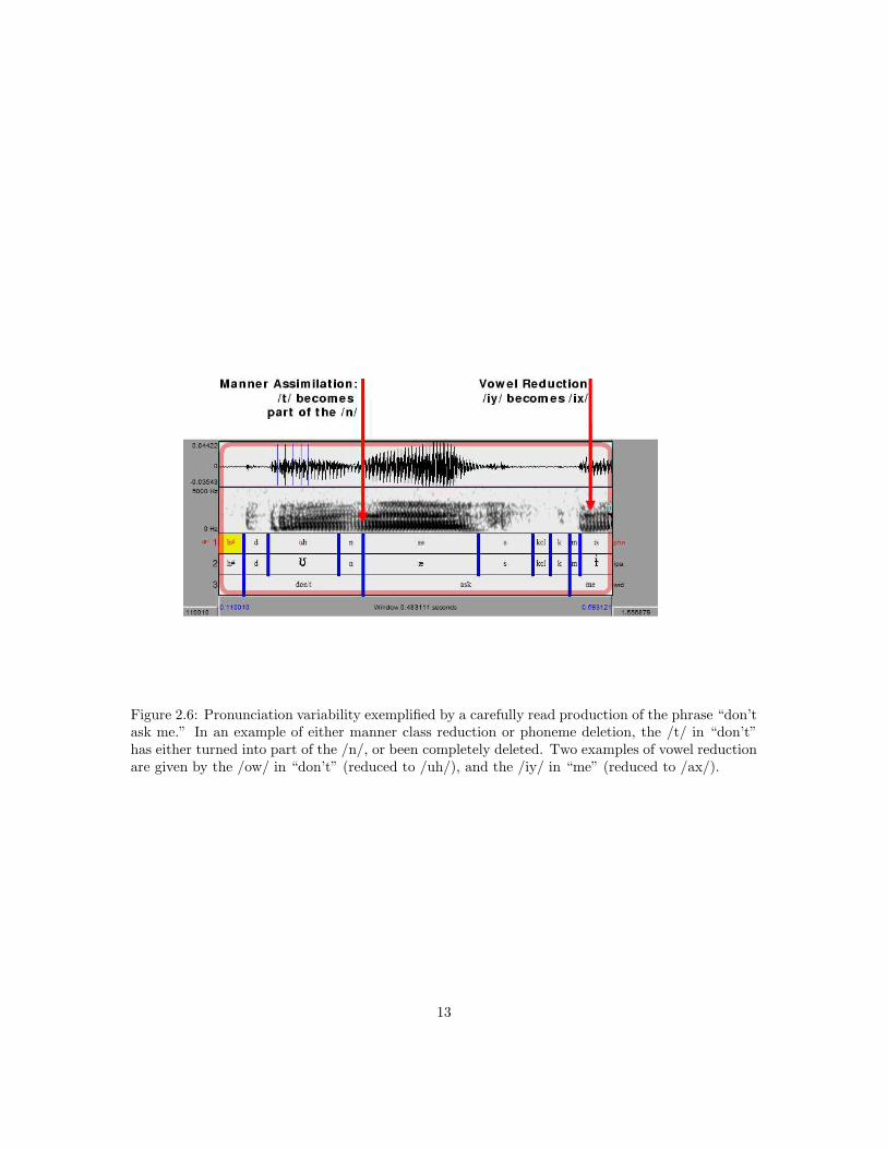
Figure 2.6: Pronunciation variability exemplified by a carefully read production of the phrase “don’task me.” In an example of either manner class reduction or phoneme deletion, the /t/ in “don’t”has either turned into part of the /n/, or been completely deleted. Two examples of vowel reductionare given by the /ow/ in “don’t” (reduced to /uh/), and the /iy/ in “me” (reduced to /ax/).

13

In 1975, Goldsmith proposed a representation called “autosegmental phonology” that modelsreduction and assimilation phenomena by extending the temporal range of some distinctive features,while deleting others [58, 36]. For example, the deletion of /t/ in “don’t ask” would not be modeled asa complete deletion; instead, the timing node (root node) of the /t/ segment would delete its bindingto the feature [-nasal], and bind instead to the feature [+nasal] of the preceding /n/. Autosegmentalphonology eliminates some of the rule sequencing requirements of the Chomsky & Halle model, butnot all.

In the early 1990s, Browman and Goldstein proposed a dramatically revised version of autoseg-mental phonology called “articulatory phonology” [24]. The articulatory phonology model is specifi-cally designed to address conversational speech phenomena such as place assimilation, manner classreduction, phoneme and syllable deletion, etcetera. For the purpose of explaining such conver-sational speech phenomena, the articulatory phonology model completely eliminates phonologicalrules, phonological rule sequencing, and distinctive features as heretofore understood. In their place,articulatory phonology proposes two types of psychologically motivated units: (1) gestures, and (2)tract variables. “Tract variables” are continuous-valued, mental estimates of the positions of thespeech production articulators (lips, tongue tip, tongue body, velum, glottis). “Gestures” are goals.For example, the gesture “TB-CLO” specifies a goal: the tongue body should close.

In articulatory phonology, pronunciation variability in casual speech is never caused by thedeletion or modification of gestures; if a mental planning unit (a “gesture”) is part of the mentallexicon during careful read speech, then the same mental planning unit is present in the plan forproduction of rapid conversational speech. Instead of modifying the mental lexicon for every newspeaking style, articulatory phonology proposes that all pronunciation variability is explained by (1)changes in the timing of the gestures, that affect (2) the real-time mapping from gestures (discrete)to tract variables (continuous) [143, 123]. Fig 2.7 shows, for example, the production of the phrase“don’t ask” in canonical and reduced form. In canonical form, the /n/, /t/, /ae/ sequence isimplemented by a series of glottis control gestures: GL-CRIT (glottis vibrating) for the /n/, followedby GL-CLO (glottal stop) for the /t/, followed by GL-CRIT for the /ae/. In reduced form, the GL-CRIT and GL-CLO gestures overlap, therefore the glottis never completely stops vibrating. Thearticulatory phonology model predicts that, in this phrase, glottal vibration may be reduced slightlyeven if it does not completely stop, i.e., the /t/ may be partly deleted rather than fully deleted. Thewaveform shown in Fig. 2.6 shows some evidence of a partly deleted /t/, in that the amplitude ofvoicing decreases toward the end of the /n/.

2.4 Empirical Study of Pronunciation Variability

The field of speech recognition has enabled empirical studies of pronunciation variability on a scalerather larger than the scale of most previous phonological work. Empirical study of pronunciationvariability requires that a certain amount of material be manually annotated and segmented in orderto insure that the patterns observed are not an artifact of machine models. Such annotations havebeen performed, initially as a part of the 1996 and 1997 Johns Hopkins summer workshops (1996- ”Automatic Learning of Word Pronunciation from Data;” 1997 - ”Pronunciation Modeling” and”Syllable-based Speech Processing”) and an additional set of material for evaluation of automaticSwitchboard transcription systems in 2000 and 2001. Initially, the manual annotation pertainedto both labeling and segmenting a portion of the corpus at the phonetic-segment level [63, 64].Ultimately, segmentation at the phonetic segment level was dropped in favor of segmentation at thesyllabic level. Systems were subsequently developed to automatically segment syllables into phoneticsegments using an hour’s worth of manually segmented material for training and the resultantsegmentation manually validated (and corrected where required). Ultimately, four hours of materialwere annotated with phonetic labels and segmented at the syllabic and phone levels. Forty minutesof this material was manually labeled with respect to syllabic emphasis (prosodic stress accent) as

14

Figure 2.7: Articulatory phonology proposes that the acoustic /t/ in “don’t ask” may be deletedwithout the deletion or alteration of any of the underlying mental speech planning or speech percep-tion units. Upper plot: in a canonical pronunciation, the /n/ and /ae/ require a GL-CRIT (glottisvibrating) gesture, while the /t/ requires a GL-CLO (glottal stop) gesture. Lower plot: in a casualpronunciation, the GL-CLO and GL-CRIT gestures overlap, therefore the glottis never completelystops vibrating.

15

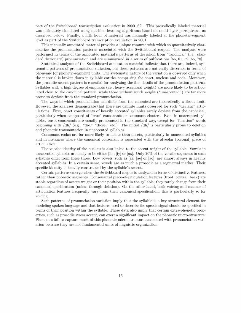
part of the Switchboard transcription evaluation in 2000 [62]. This prosodically labeled materialwas ultimately simulated using machine learning algorithms based on multi-layer perceptrons, asdescribed below. Finally, a fifth hour of material was manually labeled at the phonetic-segmentlevel as part of the Switchboard transcription evaluation in 2001.

This manually annotated material provides a unique resource with which to quantitatively char-acterize the pronunciation patterns associated with the Switchboard corpus. The analyses wereperformed in terms of the annotated material’s patterns of deviation from “canonical” (i.e., stan-dard dictionary) pronunciation and are summarized in a series of publications [65, 61, 59, 66, 78].

Statistical analyses of the Switchboard annotation material indicate that there are, indeed, sys-tematic patterns of pronunciation variation, but these patterns are not easily discerned in terms ofphonemic (or phonetic-segment) units. The systematic nature of the variation is observed only whenthe material is broken down in syllabic entities comprising the onset, nucleus and coda. Moreover,the prosodic accent pattern is essential for analyzing the fine details of the pronunciation patterns.Syllables with a high degree of emphasis (i.e., heavy accentual weight) are more likely to be articu-lated close to the canonical pattern, while those without much weight (“unaccented”) are far moreprone to deviate from the standard pronunciation.

The ways in which pronunciation can differ from the canonical are theoretically without limit.However, the analyses demonstrate that there are definite limits observed for such “deviant” artic-ulations. First, onset constituents of heavily accented syllables rarely deviate from the canonical,particularly when composed of “true” consonants or consonant clusters. Even in unaccented syl-lables, onset consonants are usually pronounced in the standard way, except for “function” wordsbeginning with /dh/ (e.g., “the,” “those,” etc.). The initial /dh/ is particularly prone to deletionand phonetic transmutation in unaccented syllables.

Consonant codas are far more likely to delete than onsets, particularly in unaccented syllablesand in instances where the canonical consonant is associated with the alveolar (coronal) place ofarticulation.

The vocalic identity of the nucleus is also linked to the accent weight of the syllable. Vowels inunaccented syllables are likely to be either [ih], [iy] or [ax]. Only 20% of the vocalic segments in suchsyllables differ from these three. Low vowels, such as [aa] [ae] or [ao], are almost always in heavilyaccented syllables. In a certain sense, vowels are as much a prosodic as a segmental marker. Theirspecific identity is heavily constrained by the syllable’s accent.

Certain patterns emerge when the Switchboard corpus is analyzed in terms of distinctive features,rather than phonetic segments. Consonantal place-of-articulation features (front, central, back) arestable regardless of accent weight or their position within the syllable; they rarely change from theircanonical specification (unless through deletion). On the other hand, both voicing and manner ofarticulation features frequently vary from their canonical specification; this is particularly so forvoicing.

Such patterns of pronunciation variation imply that the syllable is a key structural element formodeling spoken language and that features used to describe the speech signal should be specified interms of their position within the syllable. These data also imply that certain extra-phonetic prop-erties, such as prosodic stress accent, can exert a significant impact on the phonetic micro-structure.Phonemes fail to capture much of this phonetic micro-structure associated with pronunciation vari-ation because they are not fundamental units of linguistic organization.

16

Chapter 3

Distinctive Feature Definition

Although the primary goal of the research described in this report was the development of speechrecognition systems based on distinctive features, we discovered early in the planning process thatour technological development effort requires careful reconsideration of our scientific foundation. Atleast three different sets of distinctive features were developed for the purpose of this workshop.The “distinctive features,” used for the training and testing of SVM classifiers, were motivatedprimarily by the speech perception work of Miller and Nicely [118] and the phonological work ofStevens and Keyser [92]. The “articulatory features,” motivated by the demands of pronunciationvariability, were based primarily on the “tract variables” of Browman and Goldstein [24]. The“entropes” were motivated by the requirements of automatic speech recognition: specifically, bythe requirement of lexical discriminability. Theoretical foundations for the entropes were developedduring the workshop, and there was therefore no time to test the entropes in a complete speechrecognition system. Sections 3.1 and 3.2 describe the distinctive features and the entropes; thearticulatory features are described in Chapter 5 and Appendix A.2, and the mapping from distinctivefeatures to articulatory features is given in Appendix A.3.

3.1 Distinctive Features

Classifiers were trained to perform binary distinctive feature classifications, or binary feature-changedetection. For the purposes of this workshop, a “distinctive feature” was initially defined very looselyto be “any binary division of the set of English phonemes” (some sub-phonemic distinctions werealso tested; see Sec. 4.7). From this very broad definition of the term “distinctive feature,” specificdistinctive features were selected for experimental test based on the following considerations.

Distinctive feature definitions were drawn from primarily two sources. First, consonants wereclassified according to the Miller & Nicely distinctions [118] (although we changed the names oftheir distinctions, in order to match Chomsky & Halle [35]). In order of decreasing perceptualrobustness (as measured by Miller & Nicely, and supported by [11] and others), the consonantfeatures are: [sonorant, voiced, continuant, strident, palatal, labial].1 Second, vowelswere classified as in [154]: [high, low, back, ATR, CP].2 Finally, the feature [syllabic] was

1Reduction of /g/ and /k/ to /y/ is extremely common in conversational telephone speech data. For example, inone error analysis performed during WS04, 9 out of 10 utterances of the phrase “I guess” were found to have beenproduced using a /y/ in place of the /g/, and one utterance of the phrase “like a” was produced using a /y/ in placeof the /k/. In order to compactly represent this common reduction, the places of articulation of /y/, /sh/, /zh/, /ch/,/jh/, /g/, and /k/ were coded using the same feature, written in this report as [+palatal]. The standard phoneticdescription of American English /k/, /g/, and /ng/ claims that these sounds are velar in back-vowel context, andpalatal in front vowel context [158]; since the distinction is sub-phonemic in English, we claim that adoption of thecommon feature “palatal” does no harm.

2ATR=advanced tongue root, CP=constricted pharynx.

17

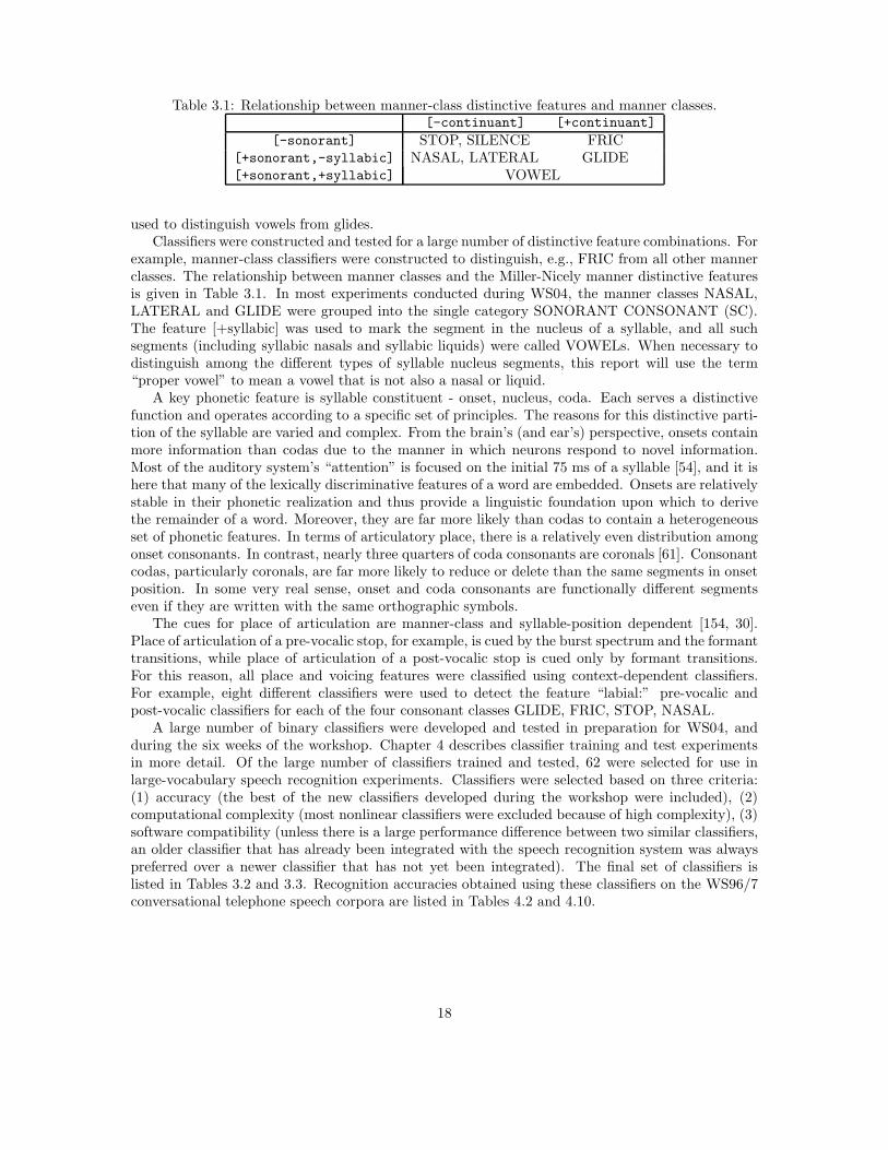
Table 3.1: Relationship between manner-class distinctive features and manner classes.[-continuant] [+continuant]

[-sonorant] STOP, SILENCE FRIC[+sonorant,-syllabic] NASAL, LATERAL GLIDE[+sonorant,+syllabic] VOWEL

used to distinguish vowels from glides.Classifiers were constructed and tested for a large number of distinctive feature combinations. For

example, manner-class classifiers were constructed to distinguish, e.g., FRIC from all other mannerclasses. The relationship between manner classes and the Miller-Nicely manner distinctive featuresis given in Table 3.1. In most experiments conducted during WS04, the manner classes NASAL,LATERAL and GLIDE were grouped into the single category SONORANT CONSONANT (SC).The feature [+syllabic] was used to mark the segment in the nucleus of a syllable, and all suchsegments (including syllabic nasals and syllabic liquids) were called VOWELs. When necessary todistinguish among the different types of syllable nucleus segments, this report will use the term“proper vowel” to mean a vowel that is not also a nasal or liquid.

A key phonetic feature is syllable constituent - onset, nucleus, coda. Each serves a distinctivefunction and operates according to a specific set of principles. The reasons for this distinctive parti-tion of the syllable are varied and complex. From the brain’s (and ear’s) perspective, onsets containmore information than codas due to the manner in which neurons respond to novel information.Most of the auditory system’s “attention” is focused on the initial 75 ms of a syllable [54], and it ishere that many of the lexically discriminative features of a word are embedded. Onsets are relativelystable in their phonetic realization and thus provide a linguistic foundation upon which to derivethe remainder of a word. Moreover, they are far more likely than codas to contain a heterogeneousset of phonetic features. In terms of articulatory place, there is a relatively even distribution amongonset consonants. In contrast, nearly three quarters of coda consonants are coronals [61]. Consonantcodas, particularly coronals, are far more likely to reduce or delete than the same segments in onsetposition. In some very real sense, onset and coda consonants are functionally different segmentseven if they are written with the same orthographic symbols.

The cues for place of articulation are manner-class and syllable-position dependent [154, 30].Place of articulation of a pre-vocalic stop, for example, is cued by the burst spectrum and the formanttransitions, while place of articulation of a post-vocalic stop is cued only by formant transitions.For this reason, all place and voicing features were classified using context-dependent classifiers.For example, eight different classifiers were used to detect the feature “labial:” pre-vocalic andpost-vocalic classifiers for each of the four consonant classes GLIDE, FRIC, STOP, NASAL.

A large number of binary classifiers were developed and tested in preparation for WS04, andduring the six weeks of the workshop. Chapter 4 describes classifier training and test experimentsin more detail. Of the large number of classifiers trained and tested, 62 were selected for use inlarge-vocabulary speech recognition experiments. Classifiers were selected based on three criteria:(1) accuracy (the best of the new classifiers developed during the workshop were included), (2)computational complexity (most nonlinear classifiers were excluded because of high complexity), (3)software compatibility (unless there is a large performance difference between two similar classifiers,an older classifier that has already been integrated with the speech recognition system was alwayspreferred over a newer classifier that has not yet been integrated). The final set of classifiers islisted in Tables 3.2 and 3.3. Recognition accuracies obtained using these classifiers on the WS96/7conversational telephone speech corpora are listed in Tables 4.2 and 4.10.

18

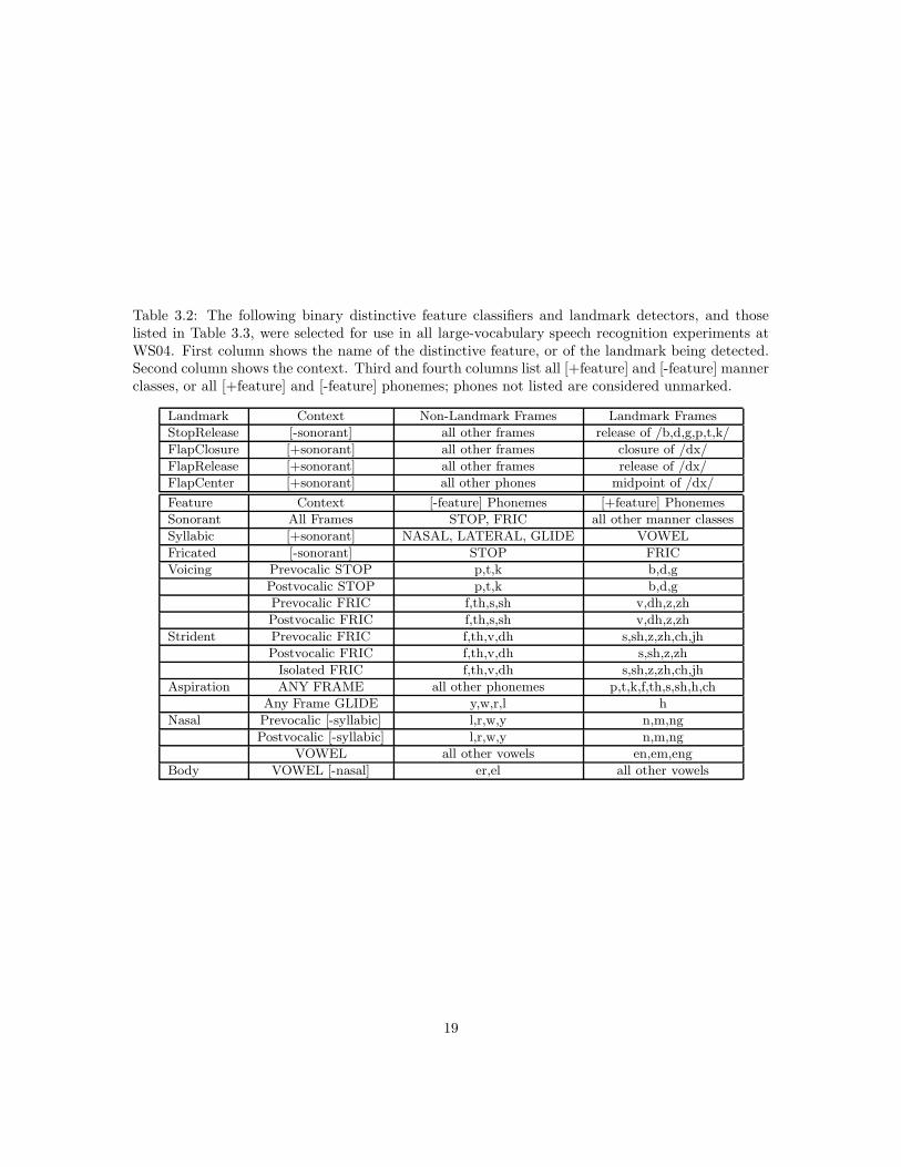
Table 3.2: The following binary distinctive feature classifiers and landmark detectors, and thoselisted in Table 3.3, were selected for use in all large-vocabulary speech recognition experiments atWS04. First column shows the name of the distinctive feature, or of the landmark being detected.Second column shows the context. Third and fourth columns list all [+feature] and [-feature] mannerclasses, or all [+feature] and [-feature] phonemes; phones not listed are considered unmarked.

Landmark Context Non-Landmark Frames Landmark Frames

StopRelease [-sonorant] all other frames release of /b,d,g,p,t,k/

FlapClosure [+sonorant] all other frames closure of /dx/

FlapRelease [+sonorant] all other frames release of /dx/

FlapCenter [+sonorant] all other phones midpoint of /dx/

Feature Context [-feature] Phonemes [+feature] Phonemes

Sonorant All Frames STOP, FRIC all other manner classes

Syllabic [+sonorant] NASAL, LATERAL, GLIDE VOWEL

Fricated [-sonorant] STOP FRIC

Voicing Prevocalic STOP p,t,k b,d,g

Postvocalic STOP p,t,k b,d,g

Prevocalic FRIC f,th,s,sh v,dh,z,zh

Postvocalic FRIC f,th,s,sh v,dh,z,zh

Strident Prevocalic FRIC f,th,v,dh s,sh,z,zh,ch,jh

Postvocalic FRIC f,th,v,dh s,sh,z,zh

Isolated FRIC f,th,v,dh s,sh,z,zh,ch,jh

Aspiration ANY FRAME all other phonemes p,t,k,f,th,s,sh,h,ch

Any Frame GLIDE y,w,r,l h

Nasal Prevocalic [-syllabic] l,r,w,y n,m,ng

Postvocalic [-syllabic] l,r,w,y n,m,ng

VOWEL all other vowels en,em,eng

Body VOWEL [-nasal] er,el all other vowels

19

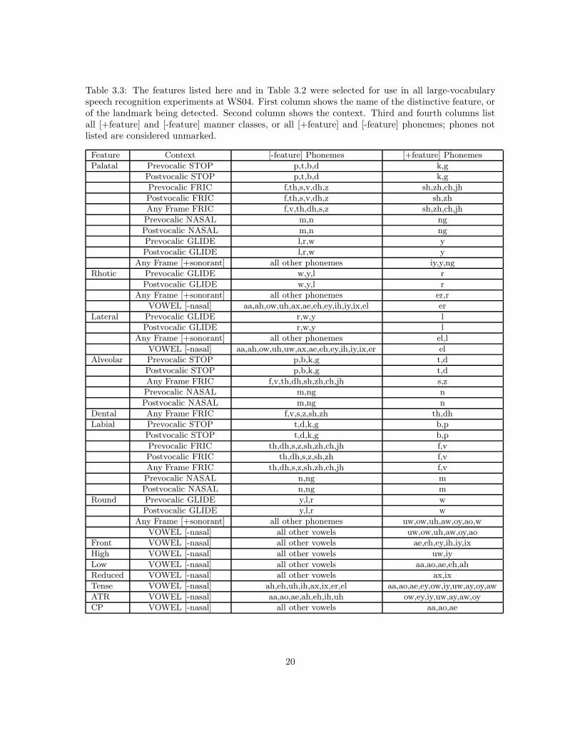
Table 3.3: The features listed here and in Table 3.2 were selected for use in all large-vocabularyspeech recognition experiments at WS04. First column shows the name of the distinctive feature, orof the landmark being detected. Second column shows the context. Third and fourth columns listall [+feature] and [-feature] manner classes, or all [+feature] and [-feature] phonemes; phones notlisted are considered unmarked.

Feature Context [-feature] Phonemes [+feature] Phonemes

Palatal Prevocalic STOP p,t,b,d k,g

Postvocalic STOP p,t,b,d k,g

Prevocalic FRIC f,th,s,v,dh,z sh,zh,ch,jh

Postvocalic FRIC f,th,s,v,dh,z sh,zh

Any Frame FRIC f,v,th,dh,s,z sh,zh,ch,jh

Prevocalic NASAL m,n ng

Postvocalic NASAL m,n ng

Prevocalic GLIDE l,r,w y

Postvocalic GLIDE l,r,w y

Any Frame [+sonorant] all other phonemes iy,y,ng

Rhotic Prevocalic GLIDE w,y,l r

Postvocalic GLIDE w,y,l r

Any Frame [+sonorant] all other phonemes er,r

VOWEL [-nasal] aa,ah,ow,uh,ax,ae,eh,ey,ih,iy,ix,el er

Lateral Prevocalic GLIDE r,w,y l

Postvocalic GLIDE r,w,y l

Any Frame [+sonorant] all other phonemes el,l

VOWEL [-nasal] aa,ah,ow,uh,uw,ax,ae,eh,ey,ih,iy,ix,er el

Alveolar Prevocalic STOP p,b,k,g t,d

Postvocalic STOP p,b,k,g t,d

Any Frame FRIC f,v,th,dh,sh,zh,ch,jh s,z

Prevocalic NASAL m,ng n

Postvocalic NASAL m,ng n

Dental Any Frame FRIC f,v,s,z,sh,zh th,dh

Labial Prevocalic STOP t,d,k,g b,p

Postvocalic STOP t,d,k,g b,p

Prevocalic FRIC th,dh,s,z,sh,zh,ch,jh f,v

Postvocalic FRIC th,dh,s,z,sh,zh f,v

Any Frame FRIC th,dh,s,z,sh,zh,ch,jh f,v

Prevocalic NASAL n,ng m

Postvocalic NASAL n,ng m

Round Prevocalic GLIDE y,l,r w

Postvocalic GLIDE y,l,r w

Any Frame [+sonorant] all other phonemes uw,ow,uh,aw,oy,ao,w

VOWEL [-nasal] all other vowels uw,ow,uh,aw,oy,ao

Front VOWEL [-nasal] all other vowels ae,eh,ey,ih,iy,ix

High VOWEL [-nasal] all other vowels uw,iy

Low VOWEL [-nasal] all other vowels aa,ao,ae,eh,ah

Reduced VOWEL [-nasal] all other vowels ax,ix

Tense VOWEL [-nasal] ah,eh,uh,ih,ax,ix,er,el aa,ao,ae,ey,ow,iy,uw,ay,oy,aw

ATR VOWEL [-nasal] aa,ao,ae,ah,eh,ih,uh ow,ey,iy,uw,ay,aw,oy

CP VOWEL [-nasal] all other vowels aa,ao,ae

20

3.1.1 Manner of Articulation

The features Sonorant, Syllabic, Fricated, and Nasal contain manner-of-articulation informationpertinent to the articulatory mode of production - stop, fricative, nasal, liquid, glide, vowel, etc.These particular features come closest to the classical concept of the phone. Temporally, manner ofarticulation and the phone are virtually isomorphic. For this reason, it is possible to automaticallysegment a corpus, such as Switchboard, by using manner of articulation classifiers. Manner isextremely important for specifying the phonetic identity of a word. Traditionally, manner has beenidentified with a conglomeration of acoustic and articulatory properties, ranging from harmonicityto noise. But such spectral attributes are only part of manner’s distinctiveness. Equally important isthe overall energy level associated with each manner class. Stops and fricatives are intrinsically lowerin amplitude than vowels, liquids, glides and nasals. For reasons discussed below, this property alonerelegates these segments to the flanks of the syllable. They always serve as onset or coda elements andcan occur as clusters in restricted ways. Affricates are essentially stop-fricative compounds. Stopsand fricatives are the only two manner classes (in English) whose order is interchangeable withina syllable constituent (e.g., “claps” “clasp”), suggesting that they are complementary structurally.Nasals have more energy than stops and fricatives, and for this reason either may precede this mannerclass in the syllable coda (in English). Liquids and glides are almost as energetic as vowels and oftenimmediately precede or follow the vocalic nucleus. In English they are partially complementary indistribution; in the onset generally either a liquid or a glide may precede the vowel, but not both. Inthe coda, a liquid may follow a glide (but not vice versa) (one could also analyze liquids and glidesas nucleic elements, but this possibility lies outside the scope of the current report). Under certainconditions, members of either class can serve as the basis of the nucleus (along with nasals), thoughthis is relatively rare (even in spontaneous speech). Such patterns may seem arbitrary, but they’renot. For they conform to the principle of the energy arc, in which onsets rise monotonically towardsthe peak of the nucleus, and where codas descend monotonically from the nucleus to the syllable’sconclusion. The energy arc serves as a significant constraint on the sequence in which phoneticelements (particularly manner) can occur within the syllable. For this reason it is important thatsyllable structure serve as an important component of the lexical representation and can be usedboth as a validity check on the phonetic classifier output and as a means to reduce the number oflikely phonetic possibilities associated with a specific interval within the syllable.

The manner features were chosen to be lexically discriminative. Most of these features are con-ventional (stops, fricatives, nasals, glide, diphthong), but some merit discussion. The segments /th/(“thin”) /dh/ (“that”) deserve particular attention. The acoustic, articulatory, and phonologicalproperties of /th/ and /dh/ are slightly different in many respects from those of the other fricatives;for this reason, some phonological systems place these two phonemes in their own manner class,called SPIRANT. The spirants in English have a place of articulation (often called “dental”) thatis linked to the “central” or “alveolar” location, in the sense that both the dentals and the alveo-lars are produced with the tongue tip bent forward. In the notation of Chomsky and Halle [35] orStevens [154], the dentals and alveolars use a tongue blade in [+anterior] position; this is why [dh]often interchanges with [d] (in Am. English) and [th] with [z] (in Castillian Spanish). The Englishlanguage has the interesting characteristic that both stops and nasal consonants have three allowedplaces of articulation: labial, alveolar, and palato-velar. The true glides are either labial (/w/)palato-velar (/y/), or glottal (/h/), while the liquids are both alveolar (/r,l/). In a structurallyparsimonious feature system, the class fricative would also have only three places of articulation.These slots could be occupied by /f/, /s/, /sh/ (voiceless) and /v/, /z/, /zh/ (voiced). But thisleaves /th/ and /dh/ “out in the cold.” One suggestion has been to code the fricative associated withthese segments as “lingual-dental” and have four distinct places of articulation for the fricatives. Butthis “solution” fails to capture the structural relationship between these particular fricatives andother members of that class. /th/ and /dh/ are relatively rare among the world’s languages. InEnglish /dh/ most frequently occurs as the onset of certain function words such as “that” “them,

21

“the,” etc. These segments are often deleted or phonetically transmuted, in contrast to “true” stopsand fricatives, which delete very rarely at syllable onset; the only other segment in English that isfrequently deleted in syllable onset position is the aspirated glide /h/. /dh/ and /th/ are specialsegments, more phonologically akin in some ways to glides than to either fricatives or stops, andwith acoustic properties intermediate between all three of these other manner classes. The spectralproperties of spirants differ from true fricatives in exhibiting a pronounced resonance pattern, andare in this sense similar to a slightly fricated glide. In other words, these segments don’t act like“true” fricatives; in some sense, they are a hybrid or intermediary between the alveolar fricatives(/s,z/), the alveolar stops (/t,d/), and the missing English alveolar glide. In some sense, the spirantsare a manner class apart, with a unique structural role in spoken English.

The voiced fricatives (/v/, /dh/, /z/, /zh/) function differently in many ways than their unvoicedcounterparts. For example, these segments manifest nowhere near the amount of frication as /f/,/th/, /s/ and /sh/. Moreover, the rise characteristics of the voiced fricatives are quite different fromtheir unvoiced complements. The voiced versions can function as flaps, glides and even stops undercertain conditions, where is rarely the case for the unvoiced fricatives.

Another unusual manner class is the “flap.” Flaps are unusual in that their phonetic identityis mutable; a flap can implement /d/, /t/, /n/, /m/, /b/ or /v/ (in English). Acoustically, theyare characterized by a 5-40 ms depression of energy across the entire bandwidth of the spectrum.Surrounding context (always vocalic) is what imparts their phonetic identity to the listener. Flapsalways occur between an (initial) accented and an unaccented syllable (in English). Their apparentfunction is to tie two syllables together in a way that indicates their linguistic bond (usually part ofthe same word or word compound). In this sense they are not really segments, but rather syllablejunctures. For this reason, in Table 3.3, flaps are never detected as “segments;” they are alwaysdetected as “landmarks.” Three types of flap landmark detectors were developed: a “flap closure”landmark detector, a “flap release” landmark detector, and a “flap center” landmark detector.Since flaps are very short, these three landmark detectors should have similar performance, butthe experiments described in Section 4.5 will demonstrate that the flap closure landmark detectorconsistently outperforms the other two by a fairly wide margin.

The liquids are partitioned into two classes, rhotic (/r/) and lateral (/l/). The liquids can becomevowels (/er/ and /el/), or can merge with a preceding vowel to form a kind of diphthong (as in “car”or “call”). The liquids act in many ways to bind the vocalic nucleus to other parts of the syllableor to other syllables.

Similar in function, and related acoustically, are the glides. The /w/ and /y/ glides are oftenindistinguishable from vowels, particularly in coda position, where they are perceived as the trailingedge of diphthongs. In both coda and onset position they often serve to bind to another syllable.Hence, they have an intrinsic binding function that often ties syllables together into some larger unit.For this reason, their phonetic realization can be quite different that their phonemic affiliation.

/h/ is a special form of glide that is essentially a gradual onset vowel (but which can be eithervoiced or voiceless in English). In contrast to /w/ and /y/ the formant pattern is relatively staticand non-distinctive. In this sense, /h/ is a spectrally non-dynamic glide, whose energy rises fromlow to substantial over the course of the segment. /h/ is often thought to be a glottal fricative,given its unique spectral signature. In English this form occurs mostly before high, front vowels.However, a more insightful analysis associates the voicing characteristic with prosodic accent (seebelow). /h/ is essentially an aspirated onset vowel than is voiced in accented syllables, and unvoicedin less accented syllables (which accounts for why the fricated form often occurs before high, frontvowels). In syllables where the coda consonant is voiced, /h/ is usually voiced, regardless of thevowel. Thus, the voicing associated with /h/ is probably most accurately described as a syllabicphenomenon (see below), consistent with its behavior across languages (e.g., in Dutch /h/ is entirelyvoiced, while in Swedish it is always unvoiced; in classical Greek, the presence of a syllable-initial/h/ or glottal stop was written using diacritic modification of the vowel, rather than using a separatealphabetic character).

22

Vowels are partitioned into monophthongs and diphthongs. Diphthongs have a glide componentin the coda. Glides often reduce or delete, transforming a diphthong into a monophthong. Vowelsare usually associated with the nucleus, and in this capacity serve as the foundation of the syllable(see below).

3.1.2 Syllable Structure

Position within the syllable is an important phonetic property, and when used appropriately, canserve to distinguish among words reliably. The classifiers described in Table 3.3 include four differentsyllable positions: Prevocalic (syllable onset, released into a vowel or glide), Postvocalic (syllablecoda, closed from a vowel or glide), Isolated (used for fricatives that are bounded on either sideby a stop or nasal), and AnyFrame classifiers (used to label a few distinctive features whose valuecan be reliably determined in the center of the phoneme, e.g., fricative place of articulation). Mostconsonants can occur in either the onset or coda. /h/ is an exception in that in most languages(including English) it is restricted to the onset. The nasal /ng/ is restricted to the coda (in English).The phonetic properties of various segments differ depending on whether they occur in the onset orcoda. For example, the articulatory release associated with stops rarely occurs in the coda, but isquite common at syllable onset. The onset liquids differ from their coda counterparts (more so in alanguage such as German than in English). The duration of most coda consonants is substantiallyshorter than the same consonants in onset position, particularly in accented syllables.

The primary distinction between monophthongs and diphthongs concerns their distribution overthe syllable. Diphthongs have a glide component extending into the syllable coda (with a reductionin overall energy).

Junctures are elements, such as flaps and glottal stops, which serve primarily to separate syllables.These are marked explicitly as “landmarks” in Table 3.3, and as “junctures” in the system developedin Section 3.2.

3.1.3 Voicing

Voicing is generally treated as a segmental feature distinguishing voiced and unvoiced counterparts.Within the conventional distinctive feature framework, [p] differs from [b], [s] from [z] purely in termsof voicing. However, such voiced/unvoiced pairs rarely differ purely in terms of voicing, and oftenso-called voiced segments are partially unvoiced (e.g, [g] in English). Sometimes, a nominally voicedsegment may be entirely unvoiced (e.g., [z] in coda position in American English). Stevens et al.demonstrated that the phonological feature [+voiced], in American English fricatives, is not signaledby continuous voicing throughout the fricative [155]; rather, the best single acoustic measurementfor discriminating phonologically voiced vs. unvoiced fricatives was the ratio of voice bar durationdivided by total duration of the fricated segment.

In some sense, voicing can be viewed more as a syllable feature than as a segmental feature. Thenucleus of a syllable is almost always voiced (in English) and voicing variably extends to the onsetand coda depending on a number of factors. Besides segmental identity, the prosodic prominence ofthe syllable is extremely important. The latter may override segmental factors, as occurs in unvoiced/z/ in Am. English. The amount of voicing exhibited by a consonant also depends on syllable accent(e.g., pre-voicing in stops occurs in heavily accented syllables).

Voicing interacts with the energy arc in that it serves to build up energy, beginning with thesyllable’s core (i.e., nucleus). The specific energy contour of a syllable depends partly on the voicingconfiguration. Unvoiced segments generally occur only in the syllable flanks and associated withrelatively low energy (this is only stops, spirants and fricatives have voiceless segments in English).

Thus, voicing is not a primary feature distinguishing segments much of the time. It can belexically distinctive (e.g., “let” vs. “led”) so it must be indicated in some fashion, but need not beused through most of the syllable.

23

3.1.4 Place of Articulation

Place of articulation is perhaps the most discriminative feature dimension lexically, and yet it isalso among the most difficult to describe (and is without question the most difficult to automati-cally classify; see Sec. 4.6). From an articulatory perspective, place refers to the locus of maximumconstriction. Acoustically, the definition is far less precise. In onset position, the stop burst as-sociated with articulatory release contains information relevant to place classification [19]. Theformant transitions leading from the burst to the vowel can also be used to unequivocally signalplace of articulation [41], but talkers in conversational speech do not always produce such clearformant transitions [158]. Most stops can be correctly identified without the burst, and the formanttransitions are highly variable; thus it seems that these two acoustic cues are redundant and com-plementary, and it is also possible that other cues such as duration are used when the burst andformants are unclear. What is important for the current project is how to classify place of artic-ulation. From a purely articulatory perspective one would try to associate the acoustic propertieswith a specific locus of constriction. The problem with this approach is that there are 10 distinctconstriction loci in English (bilabial, labio-dental, dental, alveolar, retroflex, palatal, velar, uvular,pharyngeal, and glottal [99]). Instead of trying to identify each locus independently, it is possibleto make the place classification dependent on manner. For each manner class there are usuallyjust three places of articulation, which means that we can then label each manner class separately.From a structural perspective this simplification provides a means of representing information moredirectly than with a precise specification of place.

Place of articulation has a different meaning in vowels and consonants. In the “true” consonantsthere is a complete, or near complete constriction of the vocal apparatus, while in vowels (and suchsegments as glides and liquids) the constriction is never close to complete. The visible articulatorsprovide a significant amount of place-related information.

For both vowels and consonants, the acoustic manifestation is most closely associated with thesecond formant (or its perceptual equivalent, F2’ [75, 103]). The distinction between front, centraland back in vowels is of a different nature than the same contrast among the consonants. InEnglish, distinctions between front and central vowels, or between central and back vowels oftendon’t change the lexical identity of a word, as the same contrast would in the case of consonants;therefore Table 3.3 uses only a binary distinction ([+front] vs. [-front]) to encode place features of avowel. However, there may be an indirect relationship between consonantal and vocalic place thatcould be important in decoding words under certain conditions.

In American English, most back vowels are accompanied by lip rounding. Thus it is possible todistinguish between the central and back vowels on the basis of the feature “round.” No central vowelhas rounding (e.g., /aa/), while all truly back vowels do (e.g., /ao/). Therefore, one can use twobinary dimensions, [front] and [round], to distinguish among the three vocalic places of articulation.

Place of articulation for the glides is similar to that of the vowels, in that the [w] is associatedwith the back vowel [uh] and [y] with the front vowel [iy]. In this sense, diphthongs and glideshave two vocalic places associated with them. /h/ is usually transcribed with a glottal place ofarticulation, but the glottis is unusually wide during an /h/ rather than unusually constricted, thusit is possible to say that an /h/ has no inherent place of articulation. The liquids are essentiallyneutral with respect to place as well, as shown by the work of, e.g., Alwan and Narayanan. /l/ isproduced with a tongue tip constriction in syllable-initial position, but with a uvular constriction insyllable-final position [124]. /r/ may be produced with a retroflex tongue tip constriction, or with a“bunched” velar constriction; some talkers always use one strategy or the other, while other talkersalternate strategies depending on context [4]. Most of these constriction locations may be looselyclassified as roughly “central.”

24

3.1.5 Vowel Features

The manner class VOWEL is used in Table 3.3 to refer to any syllable nucleus segment, regardless ofthe configuration of the vocal tract. In English, syllable nuclei can be nasal consonants ([+nasal]),/er/ ([+rhotic]), /el/ ([+lateral]), or proper vowels. In increasing order of average duration andperceptual prominence, the proper vowels include schwas (/ax,ix/), lax vowels (/ih,eh,ah,uh/), tensevowels (/aa,ao,ae,ow,ey,uw,iy/), and diphthongs (/ay,aw,oy/).

Vowel height refers to the vertical position of the tongue during production of vowels and isinversely proportional to the frequency of the first formant (F1) [138]. Under certain conditions,vowel height can be lexically discriminative, as the words “pin,” “pen” and “pan” illustrate. Cor-related with vowel height is vocalic duration (high vowels are shorter than low vowels) and energy(low vowels are more intense than their higher counterparts). As described in Sections 3.2 and 4.8,there is also a strong relationship between vowel height and the syllable’s perceived prosodic promi-nence. Low vowels are usually associated with heavily stressed syllables (in English and many otherlanguages), while high vowels generally occur in unstressed syllables (in English).

In American English, vowel height has five values: tense high (/iy/, /uw/), lax mid (/ih/, /uh/),tense mid (/ey/, /ow/), lax low (/ah/, /eh/), and tense low (/aa/, /ao/, /ae/). The tense/laxdistinction has many acoustic correlates: tense vowels have longer duration and higher F1 than theirlax counterparts. Tense vowels are also produced with an offglide, that is, with formant frequenciesthat end by moving toward more extreme values (/iy/ and /ey/ end in /y/, /ow/ and /uw/ endin /w/, /aa/ and /ae/ end with extremely high F1), while lax vowels are produced with a shortoffglide in the direction of the neutral vowel /ax/ [77]. Several methods for encoding the tense/laxdistinction have been proposed; Table 3.3 uses two of these encodings, in a redundant encoding ofvowel tension. First, Table 3.3 uses the binary feature [tense] to distinguish between all tense vowelsand all lax vowels (lax=[-tense]). Second, Table 3.3 uses the feature [+ATR] (advanced tongue root)to encode those vowels with an offglide ending in /w/ or /y/, while the feature [+CP] (constrictedpharynx) labels those vowels that end with an offglide toward values of extremely high F1. Themanipulation of tongue root muscles to create phonological vowel distinctions is well attested in somewest African languages; the proposal that tongue root tension implements the tense/lax distinctionin English is still controversial, but fits certain acoustic facts reasonably well [154].

The back vowels /uw,uh,ow,ao/ are all produced with lip rounding ([+round]) in AmericanEnglish. The defining characteristic of a back vowel is its low F2 [138]. Lip rounding acts to reduceall formant frequencies [49, 156]; if lip rounding is not phonologically distinctive in any language,therefore, it may be used as a secondary feature, to enhance the distinction between front and backvowels [152]. Lip rounding is phonologically distinctive in many European languages, but the onlyvowel pair minimally distinguished by lip rounding in American English is /aa/ vs. /ao/, and manydialects fail to distinguish these two vowels; therefore lip rounding has evolved into a secondaryfeature whose primary function is to distinguish back from front vowels. The consonants /r/, /sh/,/zh/, /ch/, /jh/ are also frequently accompanied by lip rounding, apparently because roundingenhances the distinctively low F3 in these consonants [151].

3.2 Entropes

The list of features described in Section 3.1 are not exhaustive, but rather intended to provide aguide for representing words in a large vocabulary task using articulatory-acoustic features thatare likely to be lexically discriminative. However, no single list of articulatory-acoustic featureswill ever provide the capability of distinguishing among words in real-world (i.e., large-vocabulary,conversational style) task unless they are melded to a rigorous information-theoretic framework.In order to achieve this, an additional representational unit is required beyond that of “distinctivefeature” - the entrope.

25

3.2.1 The Significance of Entropy for Lexical Discrimination

The semantic, social and emotional context interacts with the phonetic properties of speech to aconsiderable degree. A set of acoustic cues subserving one function in Context X may serve a verydifferent function in Context Y, and so on. Thus, no system based entirely on acoustic landmarks canever hope to achieve effective speech recognition without integrating this approach with the conceptof entropy. In fact, the interaction between acoustic signal and task entropy has been preciselyspecified, for the comparatively simple tasks of word recognition and sentence transcription, in aseries of experiments conducted by Miller and his colleagues in the 1950s and 1960s [121, 120, 119, 3].Miller and Isard [121] demonstrated that the recognition error rate of human listeners is determinednot by the vocabulary size of the experiment, but by the grammar perplexity [121]. Human listenersrecognizer semantically anomalous sentences almost as well as regular sentences, but syntacticallyanomalous word strings are recognized with very high error rates, comparable to the error rates thatwould be achieved if a vocabulary of the same size were presented with no order constraints at all;thus, unlike automatic speech recognizers, human listeners define the entropy of the task in terms ofthe grammar of a known human language. Miller, Heise and Lichten demonstrated that, in any one-of-N isolated word recognition task, the log accuracy of human subjects approaches the entropy ofthe task (log(1/N)) at approximately -18dB SNR. At sufficiently high SNR, the error rate of humansubjects approaches a vocabulary-independent minimum error rate of about 0.5-1.5%, however, theSNR at which minimum error rate is achieved depends on the entropy of the task. The distributionof phonological information among the various distinctive features of the consonant was specifiedby the results of Miller and Nicely [118], as discussed in Chapter 2. At least three related aspectsof speech information were not addressed by Miller and his colleagues. First, they did not addresssocially realistic speech; all speech material in their experiments was read from cue sheets. Second,they did not address the interaction between prosody and acoustic phonetic information. Third, theydid not address the interaction between information and syllable structure. Traditionally, modelsof speech recognition implicitly assume that the distribution of information throughout the word isuniform. It is for this reason that words are usually represented as sequences of phonemic elements,like beads on a string. Dictionaries (as used by both humans and machines) validate this linearrepresentation; each phoneme is considered equally important in the “underlying” representation,no matter how a word may actually be pronounced in real life.

Many experiments since Miller’s time challenge the equi-entropy distribution model of humanspeech recognition. Word onsets are more perceptually stable and reliable indices to lexical identitythan either nuclei or codas [112]. Partial recall of a word or name usually retrieves the onset con-sonant, the syllable structure and prosodic-accent pattern prior to full recollection of the missingitem. Reading experiments demonstrate that consonant symbols are more critical for understand-ing a partially transcribed passage than their vocalic counterparts. Intuitively, experts in speechrecognition know that while all sounds (and symbols) are created equal, some are more equal thanothers.

From statistical analyses of the pronunciation patterns associated with the Switchboard cor-pus [65, 61] it is possible to deduce where much of the entropy lies in the spoken utterance. But theanalyses, by themselves, don’t provide a complete picture of the variation observed or its conceptualsignificance. A broad theoretical framework is required that provides a specific motivation for whywords (and word compounds) are pronounced the way they are under a variety of circumstances. Inother words, it is necessary to understand precisely why words assume the “sound shape” they doand how this sound pattern can change as a function of context.

3.2.2 What is an Entrope?

An entrope is essentially a unit of information, and can be used to distinguish one element (at avariety of representational levels) from others; the term itself was first coined in [68]. Ideally, anentrope should contribute in a measurable way to distinguishing among words and word senses. The

26

entrope need not be the same as a “bit” of information, but can assume a more finely granulated formmore suited to the structure of spoken language and human communication. In spoken language,phonemes have traditionally been treated as entropes, but this assumption is neither substantiatedby machine-recognition performance nor by statistical analyses of spoken language.

Based on considerations discussed above, we define entropes in terms of articulatory-acousticand prosodic features that serve to distinguish syllables and words. These features form the basicstructure of syllables and can be used to reliably distinguish among various word senses, includinghomonyms.

Not all entropes are of equal force. Certain entropes are more stable and provide more reliablecues for distinguishing among words than others. Place of articulation at the onset of an accentedsyllable is one of the more forceful entropes, and this particular entropic class rarely disintegratesor mutates into another form. The importance of the articulatory-place entrope is related to twofactors. First, place of articulation is the only feature that is decoded by both the auditory and visualsystems [113]. This bi-sensory stream provides an unusual degree of resilience to acoustic backgroundinterference. Second, the onset of novel events (such as accented syllables) is encoded with particularprecision by the auditory system [122, 172, 173, 42]. Most of the neural responsiveness is at thebeginning of syllables, and the phonetic structure of speech reflects this.

Place of articulation in the syllable coda is of less force than in the onset. This is largely becausethe auditory system (and the brain in general) pays far less attention to the end of events than totheir beginning (for reasons that extend far back in evolutionary time). While articulatory placecan be a salient entrope in the coda, it usually is not; and when it is, it is generally articulated withparticular force.

The importance of the place-of-articulation entrope is reflected in the fact that onsets containonly a single place of articulation no matter how many segments are contained in this portion of thesyllable. The brain has apparently learned to associate the onset with a single entropic place, andthis is a key feature used for lexical identity.

In coda position, the situation is slightly more complicated (and interesting). Usually, a singleplace of articulation is associated with the coda (as reflected in the statistical prevalence of mono-segmental codas). However, morphologically inflecting languages, such as English, may utilize thecoda place entrope to encode a separate, bound morpheme, as in: “keep,” “kept.” Here, the codain “kept” contains two separate places of articulation. This serves as a signal that the second placeis associated with a separate morpheme, carrying an entrope associated with the past-tense marker.When adding the past tense marker in this fashion is redundant with the coda place of the root word,a separate unaccented syllable is added in its place (e.g., “create,” “created”). Thus, entropes canserve to signal individual morphemes, particularly when these are bound directly to (and modify)the root. In such circumstances, the coda contains two place entropes, one that is part of the rootand serves a referential purpose, the other subserving a grammatical function.

Place of articulation can also serve an entropic function in the nucleus. This occurs principally inaccented syllables where the specific identity of the nucleus is discriminative, either in a referentialor grammatical context. In terms of morphology, it is vowel height that most closely approximatesconsonantal place (e.g., “sing,” “sung,” “sang”). But with respect to referential distinctions, bothheight and place/rounding (e.g., “hid,” “hood”) are important for distinguishing among words.

After place, manner of articulation is the most lexically discriminative feature at the phoneticlevel. Manner is intimately bound up with syllable structure and the number of manner entropesessentially defines the broad shape of the syllable. A “typical” syllable in most languages will consistof three segments with three different manner classes, typically positioned in the onset, nucleus andcoda (i.e., CVC). However, the situation can be far more complicated in a language, such as English,where syllables can assume a wide range of structural forms. In English, a single syllable can embodyinformation that many languages require several syllables to encode. The way this is done is to usemanner entropes to extend the combinatorial capacity of the syllable. The most common way thisis achieved is through consonant clusters in either the onset or the coda (or both). The additional

27

constituents in these clusters do not modify the basic place information of the consonant cluster, butrather change the context in which that information is encoded. For example, in the word “string,”the only lexically distinctive place of articulation entrope in the onset cluster is the [+alveolar] placeof the /t/; in “spring,” the only lexically distinctive place is the [+labial] place of the /p/. The/s/ and /r/ are place-neutral manner-sequence modifiers of the fundamental /t/ or /p/. But theyserve to distinguish “string” from “sting,” and “stray” from “tray.” In English, onsets and codascan absorb up to three separate manner classes. In most languages the number of manner entropesin the onset or coda number no more than two.

The phonetic realization of manner entropes associated with the syllabic nucleus is a little un-usual. The conventional wisdom is that the nucleus contains a single constituent, which is usuallyvocalic. For the present discussion, we will accept this position (which has important implicationsfor how glides and approximants are represented). In the conventional orthography, a phone such as[ow] would be considered entirely part of the nucleus. In the present discussion the glide portion ofthe diphthong is associated with the coda rather than the nucleus. This makes the glide componentof the diphthong a mirror image phonologically of [w] and [y] when these segments precede thenucleus. Within this system, [r] and [l] following vocalic nuclei are essentially coda constituents (butwhich are essentially vocalic in nature). Although they behave in many respects like vowels, theyreside in the coda, not in the nucleus. Because the coda is prone to reduction or deletion, glidesand liquids in this position often differ from the canonical pronunciation. In onset position thesesegments have a more stable status and are less likely to delete or transmute.

Vocalic manner entropes are particularly important in heavily accented syllables, where theyfunction to distinguish among words. In English, the distinction between “men” and “main” islargely based on the glide in the latter instance. Glides are particularly important in proper nameswhere the necessity to distinguish among many alternatives is paramount.

Other entropic dimensions include voicing and rounding. Both of these are far less important thanmanner and place of articulation, but can serve to distinguish words under certain circumstances.

Certain segments tend to serve primarily a binding function within and across syllables. Thesesegments—the approximants in particular—tend to bridge between syllables, providing the meansto link semantically related elements into a larger entity. For example, in English the glide portion ofdiphthongs often functions to bind with the following syllable, particularly if it begins with a vowel.Syllables beginning with a vowel tend to be lightly accented or unaccented, while diphthongs tendto occur in accented syllables. Glides can be viewed as binding operators providing an additionaltier of information regarding the prosodic relation across adjacent syllables.

The segment /r/ often functions in an analogous manner, but where the binding valence is moresubtle than most other segments. In “syrup,” the [r] functions to bind the two syllables. The acousticcues for syllabic division are distributed mostly over a restricted frequency region (2-3 kHz). Thisbinding has the effect of telling the listener that these syllables belong to the same word, and thatit should be treated as a larger unit (as most of the spectrum appears to be a single syllable). Theother approximants have comparable properties.

Manner classes with intrinsically low energy (stops and fricatives) tend to bind differently thanapproximants. The fricatives tend to maintain their phonetic integrity between syllables; theirduration and spectral configuration changes only slightly. They are essentially segments rarely usedto bind across words and syllables (though they may). Because their energy level is relatively low(particularly below 1.5 kHz) they can bind relatively transparently. Stops and nasals, when theybind, tend to transmute into flaps; both are characterized by a brief depression of energy across theentire spectrum. The energy reduction is far from total, and is designed to signal that the syllablesare part of the same unit. Onset stops and nasals rarely serve as binders. The presence of anarticulatory release is designed to offset this portion of the syllable from what preceded it.

When vowels are bound to each other in separate syllables, it is usually accomplished througheither a glide or a liquid. The intrinsic energy of these segments is close to that of vowels, so there isonly a modest modulation of energy across the syllable juncture. In this sense, manner can provide

28

useful information about the way in which adjacent syllables are joined.Certain entropes impart more information than others (at least with respect to lexical discrim-

inability). Place of articulation at the onset of accented syllables usually provides the greatestdiscriminative potential. ASR systems tend to get the onsets of words right in correctly recognizedwords [62]. The manner associated with onset segments is also important to correctly recognize. Incontrast, the specific identity of the vowel is far less important to classify precisely (for correct wordrecognition). A framework for weighting entropes can be developed that provides for optimal lexicaldisrimination and used to score each word in terms of its intrinsic entropy independent of context(as well as within the context of other words).

3.2.3 The Importance of Prosodic Accent

The (lexically) discriminative potential of a particular entrope varies, depending on semantic context.The linguistic parameter most closely associated with context is prosodic accent. The accent placedon the syllable determines the way in which entropes are realized [33, 31, 32, 38]. In this sense,accent provides an interpretive framework for the entropic constituents of the syllable, word andutterance. With the accent pattern it is easier to interpret the acoustic signal and associate it withthe abstract representations of the words stored in the lexicon (both mental or machine).

In accented syllables, entropes are likely to be realized to their full potential (what in moreconventional terminology would be referred to as “canonical” forms). The place and manner entropesare usually fully specified and the vocalic component highly distinctive. Glides and approximantsare likely to be fully articulated as well. The voiced stop consonants are an interesting case study: ashorter voice onset time (VOT) would make them sound more voiced, but a longer VOT would makethem sound more stop-like. It turns out that both voiced and unvoiced stops have longer VOT inpitch-accented syllables [38]; thus there is overlap between the VOT distributions of accented voicedstops and those of unaccented unvoiced stops.

The interesting cases pertain to lightly and unaccented syllables where the entropes are onlypartially realized. The entropic potential of the constituents within the syllable depend on the accentof the syllable. Syllables with high entropic potential tend to have a complex syllable structure (inEnglish), often with consonant clusters and glide components. Those with relatively low entropiccapacity tend to have far simpler syllable structures, often lacking a consonantal onset, and withreduced coda structure. In the extreme case, the sound shape of a word may consist only of anucleus (e.g., “a”). In most other low-entropy words, the initial constituent is a vowel, a glideor approximant. The onsets of such words are highly mutable and are therefore less likely to beassociated with high entropy in any context. In all of the most frequent lexical compounds (usuallybigrams) contain at least one word that begins with either a vowel, a glide or approximant (thelow entropy constituents). The only exceptions are instances where one or both words begin withthe segment [dh] (e.g., “that”), which in many respects behaves like an approximant in English (itfrequently deletes or reduces in unaccented syllables). In each instance, such bigrams usually containone or more unaccented syllables.

The vocalic composition of low-entropy words also tends to be non-random. Common wordsgenerally contain high vowels, even in their canonical representation. Such vocalic forms are closelyassociated with unaccented syllables.

3.2.4 Computation of Entropic Potential

From the principles enumerated above, it should be possible to compute the intrinsic entropy of anyword (at least in English) based on the base-form pronunciation. Integral to this computation isthe notion that the phonetic realization of the constituents within the syllable is determined by theaccent pattern. It is rare for more than two contiguous syllables to be of the same accent. Usually,adjacent syllables vary in their accent weight. This is because accent is an indirect reflection of the

29

information contained in the utterance, and information is non-uniformly distributed (the reasonsfor this are complex and profound, but lie beyond the scope of the present discussion - see [65, 68]for further details).

Because accent affects the entropic realization of syllables, and because there is a temporaldimension to accent, entropy is really a measure of the amount of information per unit time. Ifthe accent pattern of an utterance can be reliably characterized, it would be possible to provide apreliminary estimate of how much (lexically discriminative) information is contained within. Thestructure of entropy distributed throughout the syllable is highly constrained, as described above.For any given syllable, there are, at most, four (and usually three) places of articulation. In terms ofmanner, the number of entropes per syllable varies between one and seven, with the average rangingbetween two and three. Rounding, when it applies, is usually confined to the nucleus. Voicingusually affects only the onset and codas, but is rarely truly contrastive.

3.2.5 The Boundary Valence - Binding Syllables

Certain segments tend to serve primarily a binding function within and across syllables. Thesesegments - the approximants in particular - tend to bridge between syllables, providing the means tolink semantically related elements into a larger entity. For example, in English the glide portion ofdiphthongs often functions to bind with the following syllable, particularly if it begins with a vowel.Syllables beginning with a vowel tend to be lightly accented or unaccented, while diphthongs tendto occur in accented syllables. Glides can be viewed as binding operators providing an additionaltier of information regarding the prosodic relation across adjacent syllables.

The segment /r/ often functions in an analogous manner, but where the binding valence is moresubtle than most other segments. In “syrup,” the [r] functions to bind the two syllables. The acousticcues for syllabic division are distributed mostly over a restricted frequency region (2-3 kHz). Thisbinding has the effect of telling the listener that these syllables belong to the same word, and thatit should be treated as a larger unit (as most of the spectrum appears to be a single syllable). Theother approximants have comparable properties.

Manner classes with intrinsically low energy (stops and fricatives) tend to bind differently thanapproximants. The fricatives tend to maintain their phonetic integrity between syllables; theirduration and spectral configuration changes only slightly. They are essentially segments rarely usedto bind across words and syllables (though they may). Because their energy level is relatively low(particularly below 1.5 kHz) they can bind relatively transparently. Stops and nasals, when theybind, tend to transmute into flaps; both are characterized by a brief depression of energy across theentire spectrum. The energy reduction is far from total, and is designed to signal that the syllablesare part of the same unit. Onset stops and nasals rarely serve as binders. The presence of anarticulatory release is designed to offset this portion of the syllable from what preceded it.

When vowels are bound to each other in separate syllables, it is usually accomplished througheither a glide or a liquid. The intrinsic energy of these segments is close to that of vowels, so there isonly a modest modulation of energy across the syllable juncture. In this sense, manner can provideuseful information about the way in which adjacent syllables are joined.

3.2.6 Entropy Hierarchy

Certain entropes impart more information than others (at least with respect to lexical discrim-inability). Place of articulation at the onset of accented syllables usually provides the greatestdiscriminative potential. ASR systems tend to get the onsets of words right in correctly recognizedwords [62]. The manner associated with onset segments is also important to correctly recognize. Incontrast, the specific identity of the vowel is far less important to classify precisely (for correct wordrecognition). A framework for weighting entropes can be developed that provides for optimal lexical

30

disrimination and used to score each word in terms of its intrinsic entropy independent of context(as well as within the context of other words).

3.2.7 Automatic Generation of Pronunciation Models

The principles outlined in this report can be used to automatically generate pronunciation modelsfor large-vocabulary tasks. The key is to develop models that are based on the same features as usedby the phonetic classifiers, and to embed these within an information-theoretic framework. It is alsoimportant for a broad range of pronunciation variation to be encapsulated within the lexical models.Given the right set of units, the algorithms for generating a pronunciation lexicon will be similarto those currently in use for phoneme-based lexicons: exemplar collection, followed by pruning andmerger of lexical entries [51, 141, 157, 159, 169, 171]. The drawback of the approach is the inherentconfusability of lexical models with so many phonetic variants. In order to reduce confusability, amulti-pass recognition search could be used to prune the lexical candidates. Initially, the recognitioncould be based on the central tendencies of phonetic properties associated with words. Top-downinformation (based on n-gram statistics) could be used to prune the list of candidates still further.Finally, individual pronunciation variants could be accessed to associate the phonetic data with thelikely word.

However, none of these approaches is likely to result in significant performance gains withoutembedding the classification and pronunciation models within a fully entropic framework. Much ofthe pronciation variation observed in the Switchboard corpus reflects differential amounts of entropyassociated with various parts of syllables, words and phrases. Unless this variation is captured in asystematic way, there is little prospect of moving beyond the current HMM ASR framework.

31

Chapter 4

Landmark Detection and

Classification

This chapter describes a large number of different binary phoneme, allophone, and prosodic classifi-cation experiments performed at WS04. Section 4.1 describes related work upon which the work inthis chapter is based. Sections 4.2 and 4.3 describe resources (Section 4.2) and methods (Section 4.3)common to all experiments described in this chapter. Sections 4.4 through 4.8 provide detailed meth-ods and results for binary classification of phonemic manner class (Section 4.4), landmark presencevs. absence (Section 4.5), phoneme place of articulation (Section 4.6), vowel nasalization (Sec-tion 4.7), and prosody (Section 4.8). Section 4.9 describes a complete speech recognizer that uses adynamic programming algorithm to find the maximum a posteriori alignment of a canonical pronun-ciation with the landmarks detected in a speech signal. Finally, section 4.10 reviews and discussessome of the phoneme classification experiments and results that most strongly affected the successof landmark-based large vocabulary speech recognizers at WS04.

4.1 Related Work

Early work in automatic speech recognition included relatively sophisticated linguistic representa-tions of phonology [37, 136], syntax [7, 53], and semantics [125]. By contrast, it was often assumedthat expert knowledge of acoustic phonetics could add little to the knowledge automatically acquiredby a dynamic programming [81], finite state automaton [83], or HMM [6] algorithm; the success ofthese algorithms was so great that Klatt proposed a model of human speech perception based onframe-based finite state automata [97]. It was frequently argued that the acoustic correlates of aphoneme are so variable and context-dependent that context-independent phoneme classification isimpossible; thus human speech perception must integrate a tremendous amount of context for evensimple phoneme perception tasks [104]. The possibility of achieving very low phoneme classificationerror rates with limited context was first demonstrated in two quite different sets of experiments:spectrogram reading experiments [178], and experiments with neural networks [165]. Later experi-ments with hybrid neural-network/HMM systems hinted at the strong correlation between phonemeerror rate and word error rate of an automatic speech recognizer [115, 9, 22, 21], leading to a re-newed engineering focus on the linguistic discipline of acoustic phonetics [10, 17]. In particular,the research at WS04 draws on a number of previous works that incorporated binary or multi-valued phonological distinctive features into a hidden Markov model or other dynamic Bayesiannetwork [45, 94, 95, 96, 93]; some of these methods will be reviewed in more detail in Section 5.2.The high correlation between the phoneme error rate and word error rates of an automatic speechrecognizer has now been empirically established by large studies of DARPA-funded prototype sys-

32

tems [64, 65]. Given results of these recent studies, it is now possible to say, with confidence, thatengineering efforts focused on improving the phoneme classification models in an automatic speechrecognizer will typically yield proportionate improvements in word error rate.

The “landmark-based speech recognition” approach described in this report draws on ideas ini-tially proposed by Stevens et al. [150, 153]. In 1992, Stevens and his colleagues proposed a frameworkfor automatic speech recognition based on his theory of human speech perception [153]. The algo-rithm described by Stevens begins with the detection of perceptually salient acoustic landmarks.These landmarks are of different types, including obstruent and nasal closures and releases, glideextrema, and the “steady state” center regions of vowels and syllabic consonants. Because land-marks are of different types, the detection of a landmark also specifies the values of distinctivefeatures which define the landmark type. Stevens calls distinctive features which define a land-mark type “articulator-free features,” because they can be implemented by any articulator; in his2000 proposal, the articulator-free features are [vowel, glide, consonant, sonorant, continuant, stri-dent]. Using knowledge-based algorithms, Liu was able to detect closure and release of [-sonorant]consonants with an accuracy of approximately 95% [106, 105]. Liu detected closure and release of[+sonorant,-continuant] consonants (nasal consonants) with an accuracy of about 89%, and Chen [34]was able to detect nasalization in vowels adjacent to 94% of all nasal consonants. Howitt [79] useda multi-layer perceptron to detect vowel landmarks with 93% accuracy. Espy-Wilson developedsemivowel detectors with similarly high accuracy [48].

Glass and Zue [56] proposed the use of a simple spectral-change metric to detect phoneme segmentboundaries in the SUMMIT system, and Halberstadt and Glass [71, 72] used the SUMMIT segmentboundaries to anchor phoneme classification in a landmark-based system. Both papers propose thatthe landmark detector should be allowed to generate a large number of false landmarks, in order toavoid the false rejection of any true landmarks. In the system proposed by Halberstadt and Glass, alexical alignment program finds the best match between each sentence candidate and the proposedlist of landmarks. As a by-product of lexical alignment, the program determines which landmarksare true segment-boundary landmarks, and which are segment-internal landmarks.

Landmark-based and segment-based speech recognition methods have been incorporated intohidden Markov models in a number of ways. Ostendorf et al. described a large family of methods formodeling variability in the duration and temporal sequencing of phonetic events; both segment-basedand hidden Markov models were shown to be special cases of the general family of methods [137].Bilmes et al. [15] used an HMM with models of phonetic auditory events (avents) separated byphoneme-independent steady state models, and achieved a 1.2% word error rate on the DIGITS+database (ten digits plus “oh,” “no,” and “yes”). Word error rate did not increase as much in noiseas a standard speech recognizer; at 10dB SNR, word error rate was 8.1%. Omar, Hasegawa-Johnson,and Levinson created an explicit duration hidden Markov model (EDHMM) with special probabilitydensity models of phoneme boundaries; stop consonant recognition error rate was reduced by a factorof three, but over-all phoneme recognition error rate was unchanged because of degraded recognitionperformance for vowels and glides [135]. The inappopriateness of standard MFCC features for alandmark-based speech recognizer motivated Omar and Hasegawa-Johnson to develop a generalizedmaximum likelihood nonlinear acoustic feature transformation for use in mixture Gaussian HMMsand EDHMMs [133, 134].

Niyogi and Ramesh trained radial basis function support vector machines (RBF SVMs) to detectstop release segments in the TIMIT database [128, 126]. For the same level of false acceptances(about 7%), the RBF stop detector incurred fewer false stop rejections (21% vs. 30%) than anHMM phoneme recognizer. Niyogi and Burges [126] have shown that the nonlinear discriminantfunctions g(~x) computed using an RBF SVM have the property of imitating the perceptual magneteffect. Specifically, the distance |g(~x1)− g(~x2)| decreases as vectors ~x1 and ~x2 are moved away fromthe g(~x) = 0 separatrix. Equivalently, the sensitivity |∇g(~x)| is a monotonically decreasing functionof |g(~x)|. In the few cases that we have carefully observed, g(~x) as learned by an RBF SVM tends toresemble an arctangent nonlinearity along the direction orthogonal to the separatrix, and therefore

33

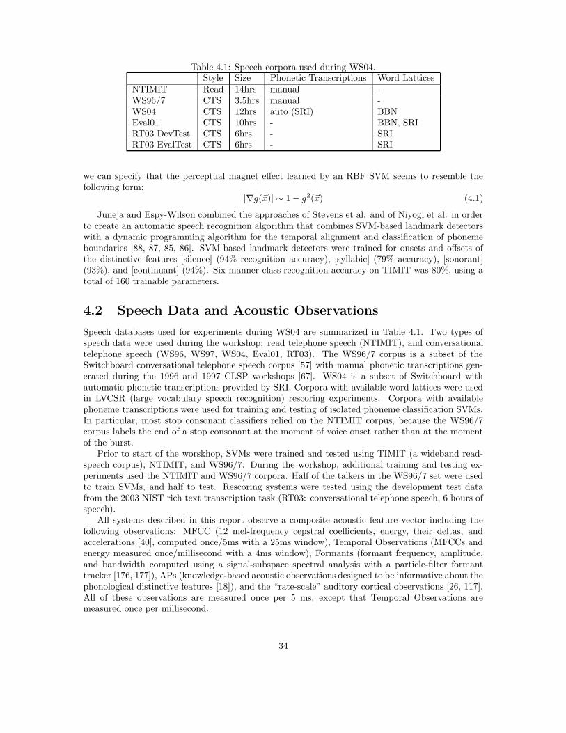
Table 4.1: Speech corpora used during WS04.Style Size Phonetic Transcriptions Word Lattices

NTIMIT Read 14hrs manual -WS96/7 CTS 3.5hrs manual -WS04 CTS 12hrs auto (SRI) BBNEval01 CTS 10hrs - BBN, SRIRT03 DevTest CTS 6hrs - SRIRT03 EvalTest CTS 6hrs - SRI

we can specify that the perceptual magnet effect learned by an RBF SVM seems to resemble thefollowing form:

|∇g(~x)| ∼ 1 − g2(~x) (4.1)

Juneja and Espy-Wilson combined the approaches of Stevens et al. and of Niyogi et al. in orderto create an automatic speech recognition algorithm that combines SVM-based landmark detectorswith a dynamic programming algorithm for the temporal alignment and classification of phonemeboundaries [88, 87, 85, 86]. SVM-based landmark detectors were trained for onsets and offsets ofthe distinctive features [silence] (94% recognition accuracy), [syllabic] (79% accuracy), [sonorant](93%), and [continuant] (94%). Six-manner-class recognition accuracy on TIMIT was 80%, using atotal of 160 trainable parameters.

4.2 Speech Data and Acoustic Observations

Speech databases used for experiments during WS04 are summarized in Table 4.1. Two types ofspeech data were used during the workshop: read telephone speech (NTIMIT), and conversationaltelephone speech (WS96, WS97, WS04, Eval01, RT03). The WS96/7 corpus is a subset of theSwitchboard conversational telephone speech corpus [57] with manual phonetic transcriptions gen-erated during the 1996 and 1997 CLSP workshops [67]. WS04 is a subset of Switchboard withautomatic phonetic transcriptions provided by SRI. Corpora with available word lattices were usedin LVCSR (large vocabulary speech recognition) rescoring experiments. Corpora with availablephoneme transcriptions were used for training and testing of isolated phoneme classification SVMs.In particular, most stop consonant classifiers relied on the NTIMIT corpus, because the WS96/7corpus labels the end of a stop consonant at the moment of voice onset rather than at the momentof the burst.

Prior to start of the worskhop, SVMs were trained and tested using TIMIT (a wideband read-speech corpus), NTIMIT, and WS96/7. During the workshop, additional training and testing ex-periments used the NTIMIT and WS96/7 corpora. Half of the talkers in the WS96/7 set were usedto train SVMs, and half to test. Rescoring systems were tested using the development test datafrom the 2003 NIST rich text transcription task (RT03: conversational telephone speech, 6 hours ofspeech).

All systems described in this report observe a composite acoustic feature vector including thefollowing observations: MFCC (12 mel-frequency cepstral coefficients, energy, their deltas, andaccelerations [40], computed once/5ms with a 25ms window), Temporal Observations (MFCCs andenergy measured once/millisecond with a 4ms window), Formants (formant frequency, amplitude,and bandwidth computed using a signal-subspace spectral analysis with a particle-filter formanttracker [176, 177]), APs (knowledge-based acoustic observations designed to be informative about thephonological distinctive features [18]), and the “rate-scale” auditory cortical observations [26, 117].All of these observations are measured once per 5 ms, except that Temporal Observations aremeasured once per millisecond.

34

4.3 SVM Computation of Posterior Probabilities

Several hundred SVMs were trained, using linear and RBF kernels; 62 were selected for use in thepronunciation models (Sec. 3.1). Three SVM toolkits were used to train and test all SVMs: SVM-light [84], libSVM [29], and SVMPath [73]. Acoustic feature inputs were selected separately for eachof the 62 classifiers, but generally included between 3 and 30 acoustic observations for manner clas-sification, and between 500 and 2000 acoustic observations for place or voicing classification. It wasdiscovered that place of articulation classifiers typically improve with every increase in the acousticfeature vector dimension, provided that the new observations are not completely determined by ex-isting observations, and provided that the dimension of the acoustic feature vector does not exceedroughly 17% of the number of training vectors. Prior to the start of the workshop, classification errorrates of most manner features were already at a very low level [85], but classification error rates ofmost place and voicing features were inadequate for speech recognition purposes. During the courseof the workshop, classification error rates of all place and voicing features fell by 10-50%, through acombination of improved selection of acoustic observations and improved classifier training methods.Error of nasal place classifiers, for example, fell by 49%; error rate of stop place classifiers fell by21%.

As described in Appendix A.1, each SVM is trained to compute a real-valued linear or nonlineardiscriminant function, gj(Xt), where j is the index of the distinctive feature, and Xt is a vectorof observations, including possibly MFCCs, Temporal Features, Formants, APs, and Rate-scaleobservations from a sequence of up to 17 consecutive or non-consecutive 5ms measurement framesin the vicinity of frame t.

The discriminants are mapped to pseudo-posteriors using a histogram. If N(gj , dj = 1) is thenumber of positive training examples of distinctive feature dj for which the SVM discriminant hada value of gj , the histogram posterior estimate is given by

q(dj = 1|gj) =N(gj , dj = 1)

N(gj , dj = 1) + N(gj , dj = −1)

Histogram counts are trained using a corpus with equal numbers of positive and negative examples,so that the pseudo-posterior q(dj |gj) is proportional to the true likelihood p(gj |dj). Posterior prob-abilities of some manner features are computed independently of the settings of all other distinctivefeatures. Posterior probabilities of place and voicing features are computed using context-dependentSVMs, meaning that a bank of SVMs and a corresponding bank of histograms are trained to estimatep(dj(t) = 1|Xt, L(t)) for every possible value of L(t), where L(t) specifies that t is a landmark of aparticular type (stop release, stop closure, fricative release, etcetera). Specific context dependenciesof each classifier are listed in Table 3.3.

4.4 Frame-Based Manner Classification

The core of all landmark-based speech recognition systems developed during WS04 was a set ofSVMs trained to label the manner class of each 5ms measurement frame. Manner class featuresincluded [sonorant], [syllabic], and [fricated]. These classifiers, and the stop release landmarkdetector, were trained and tested extensively prior to the start of WS04. Additional manner classfeatures were trained and tested during WS04.

The first set of manner classification experiments was done, prior to the workshop, using twoacoustic feature sets: an MFCC-based feature set (39 coefficients, 12MFCCs+E+delta+acceleration),and an AP feature set (42 acoustic-phonetic parameters). Results are given in Table 4.2. Inthis experiment, [+sonorant] samples include the frames of vowels, nasals, liquids and glides.[-sonorant] samples include the frames of stops and fricatives. Note that [-sonorant] samples donot include silence frames because a hierarchical structure is assumed, that is, speech-silence classi-fication is assumed as a first step. The StopRelease detector is trained using stop burst frames as

35

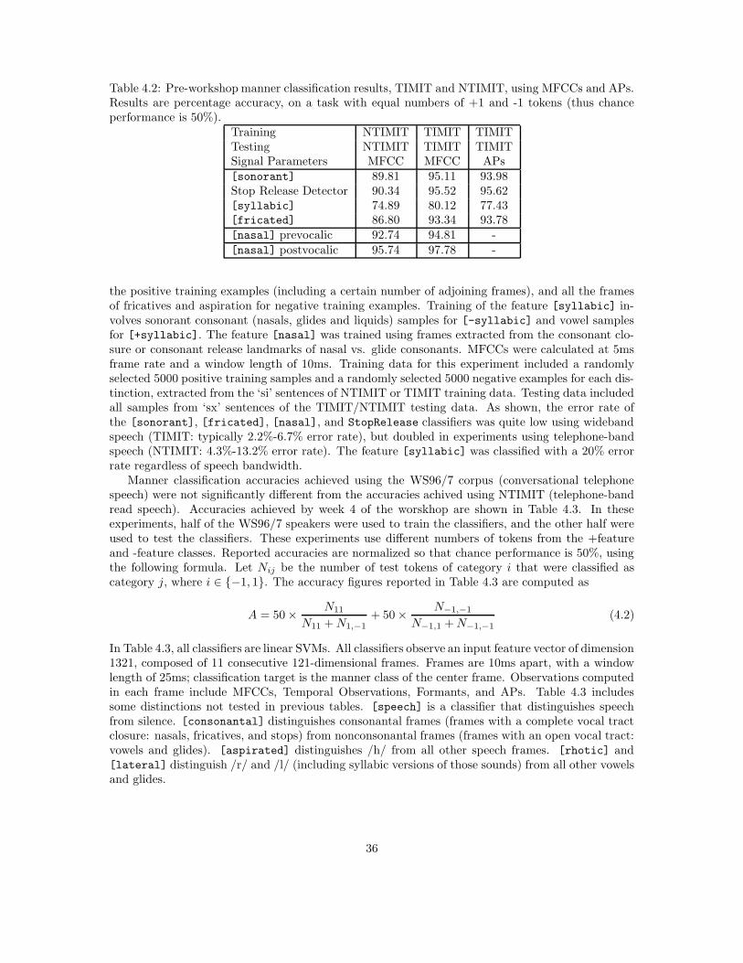
Table 4.2: Pre-workshop manner classification results, TIMIT and NTIMIT, using MFCCs and APs.Results are percentage accuracy, on a task with equal numbers of +1 and -1 tokens (thus chanceperformance is 50%).

Training NTIMIT TIMIT TIMITTesting NTIMIT TIMIT TIMITSignal Parameters MFCC MFCC APs[sonorant] 89.81 95.11 93.98Stop Release Detector 90.34 95.52 95.62[syllabic] 74.89 80.12 77.43[fricated] 86.80 93.34 93.78[nasal] prevocalic 92.74 94.81 -[nasal] postvocalic 95.74 97.78 -

the positive training examples (including a certain number of adjoining frames), and all the framesof fricatives and aspiration for negative training examples. Training of the feature [syllabic] in-volves sonorant consonant (nasals, glides and liquids) samples for [-syllabic] and vowel samplesfor [+syllabic]. The feature [nasal] was trained using frames extracted from the consonant clo-sure or consonant release landmarks of nasal vs. glide consonants. MFCCs were calculated at 5msframe rate and a window length of 10ms. Training data for this experiment included a randomlyselected 5000 positive training samples and a randomly selected 5000 negative examples for each dis-tinction, extracted from the ‘si’ sentences of NTIMIT or TIMIT training data. Testing data includedall samples from ‘sx’ sentences of the TIMIT/NTIMIT testing data. As shown, the error rate ofthe [sonorant], [fricated], [nasal], and StopRelease classifiers was quite low using widebandspeech (TIMIT: typically 2.2%-6.7% error rate), but doubled in experiments using telephone-bandspeech (NTIMIT: 4.3%-13.2% error rate). The feature [syllabic] was classified with a 20% errorrate regardless of speech bandwidth.

Manner classification accuracies achieved using the WS96/7 corpus (conversational telephonespeech) were not significantly different from the accuracies achived using NTIMIT (telephone-bandread speech). Accuracies achieved by week 4 of the worskhop are shown in Table 4.3. In theseexperiments, half of the WS96/7 speakers were used to train the classifiers, and the other half wereused to test the classifiers. These experiments use different numbers of tokens from the +featureand -feature classes. Reported accuracies are normalized so that chance performance is 50%, usingthe following formula. Let Nij be the number of test tokens of category i that were classified ascategory j, where i ∈ {−1, 1}. The accuracy figures reported in Table 4.3 are computed as

A = 50 ×N11

N11 + N1,−1+ 50 ×

N−1,−1

N−1,1 + N−1,−1(4.2)

In Table 4.3, all classifiers are linear SVMs. All classifiers observe an input feature vector of dimension1321, composed of 11 consecutive 121-dimensional frames. Frames are 10ms apart, with a windowlength of 25ms; classification target is the manner class of the center frame. Observations computedin each frame include MFCCs, Temporal Observations, Formants, and APs. Table 4.3 includessome distinctions not tested in previous tables. [speech] is a classifier that distinguishes speechfrom silence. [consonantal] distinguishes consonantal frames (frames with a complete vocal tractclosure: nasals, fricatives, and stops) from nonconsonantal frames (frames with an open vocal tract:vowels and glides). [aspirated] distinguishes /h/ from all other speech frames. [rhotic] and[lateral] distinguish /r/ and /l/ (including syllabic versions of those sounds) from all other vowelsand glides.

36

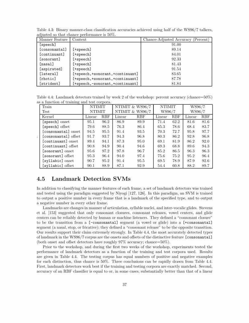
Table 4.3: Binary manner-class classification accuracies achieved using half of the WS96/7 talkers,adjusted so that chance performance is 50%.Manner Feature Context Chance-Adjusted Accuracy (Percent)[speech] 91.00[consonantal] [+speech] 89.14[continuant] [+speech] 84.01[sonorant] [+speech] 92.33[nasal] [+speech] 81.43[aspirated] [+speech] 91.54[lateral] [+speech,+sonorant,+continuant] 83.65[rhotic] [+speech,+sonorant,+continuant] 87.78[strident] [+speech,-sonorant,+continuant] 81.84

Table 4.4: Landmark detectors trained by week 2 of the workshop: percent accuracy (chance=50%)as a function of training and test corpora.

.

Train NTIMIT NTIMIT & WS96/7 NTIMIT WS96/7Test NTIMIT NTIMIT & WS96/7 WS96/7 WS96/7Kernel Linear RBF Linear RBF Linear RBF Linear RBF[speech] onset 95.1 96.2 86.9 89.9 71.4 62.2 81.6 81.6[speech] offset 79.6 88.5 76.3 86.4 65.3 78.6 68.4 83.7[consonantal] onset 94.5 95.5 91.4 93.5 70.3 72.7 95.8 97.7[consonantal] offset 91.7 93.7 94.3 96.8 80.3 86.2 92.8 96.8[continuant] onset 89.4 94.1 87.3 95.0 69.1 81.9 86.2 92.0[continuant] offset 90.8 94.9 90.4 94.6 69.3 68.8 89.6 94.3[sonorant] onset 95.6 97.2 97.8 96.7 85.2 86.5 96.3 96.3[sonorant] offset 95.3 96.4 94.0 97.4 75.6 75.2 95.2 96.4[syllabic] onset 90.7 95.2 91.4 95.5 69.5 78.9 87.9 92.6[syllabic] offset 90.1 88.9 87.1 92.9 54.4 60.8 88.2 89.7

4.5 Landmark Detection SVMs

In addition to classifying the manner features of each frame, a set of landmark detectors was trainedand tested using the paradigm suggested by Niyogi [127, 126]. In this paradigm, an SVM is trainedto output a positive number in every frame that is a landmark of the specified type, and to outputa negative number in every other frame.

Landmarks are changes in manner of articulation, syllable nuclei, and inter-vocalic glides. Stevenset al. [153] suggested that only consonant closures, consonant releases, vowel centers, and glidecenters can be reliably detected by human or machine listeners. They defined a “consonant closure”to be the transition from a [-consonantal] segment (a vowel or glide) into a [+consonantal]

segment (a nasal, stop, or fricative); they defined a “consonant release” to be the opposite transition.Our results support their claim extremely strongly. In Table 4.4, the most accurately detected typesof landmark in the WS96/7 corpus are the onsets and offsets of the distinctive feature [consonantal](both onset and offset detectors have roughly 97% accuracy; chance=50%).

Prior to the workshop, and during the first two weeks of the workshop, experiments tested theperformance of landmark detectors as a function of the training and test corpora used. Resultsare given in Table 4.4. The testing corpus has equal numbers of positive and negative examplesfor each distinction, thus chance is 50%. Three conclusions can be rapidly drawn from Table 4.4.First, landmark detectors work best if the training and testing corpora are exactly matched. Second,accuracy of an RBF classifier is equal to or, in some cases, substantially better than that of a linear

37

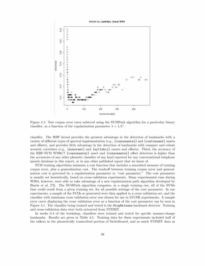
Figure 4.1: Test corpus error rates achieved using the SVMPath algorithm for a particular binaryclassifier, as a function of the regularization parameter λ = 1/C.

classifier. The RBF kernel provides the greatest advantage in the detection of landmarks with avariety of different types of spectral implementation (e.g., [consonantal] and [continuant] onsetsand offsets), and provides little advantage in the detection of landmarks with compact and robustacoustic correlates (e.g., [sonorant] and [syllabic] onsets and offsets). Third, the accuracy ofthe RBF-SVM WS96/7 [consonantal] onset and [consonantal] offset detectors is higher thanthe accuracies of any other phonetic classifier of any kind reported for any conversational telephonespeech database in this report, or in any other published report that we know of.

SVM training algorithms minimize a cost function that includes a smoothed measure of trainingcorpus error, plus a generalization cost. The tradeoff between training corpus error and general-ization cost is governed by a regularization parameter or “cost parameter.” The cost parameteris usually set heuristically, based on cross-validation experiments. Many experimental runs duringWS04, however, were able to take advantage of a new regularization path algorithm developed byHastie et al. [73]. The SVMPath algorithm computes, in a single training run, all of the SVMsthat could result from a given training set, for all possible settings of the cost parameter. In ourexperiments, a sample of the SVMs so generated were then applied to a cross validation set, and theclassifier with minimum cross validation error was chosen for use in LVCSR experiments. A sampleerror curve displaying the cross validation error as a function of the cost parameter can be seen inFigure 4.1. The classifier being trained and tested is the StopRelease landmark detector. Trainingand cross-validation data were both extracted from NTIMIT.

In weeks 2-4 of the workshop, classifiers were trained and tested for specific manner-changelandmarks. Results are given in Table 4.5. Training data for these experiments included half ofthe talkers in the phonetically transcribed portion of Switchboard, and as much NTIMIT data as

38

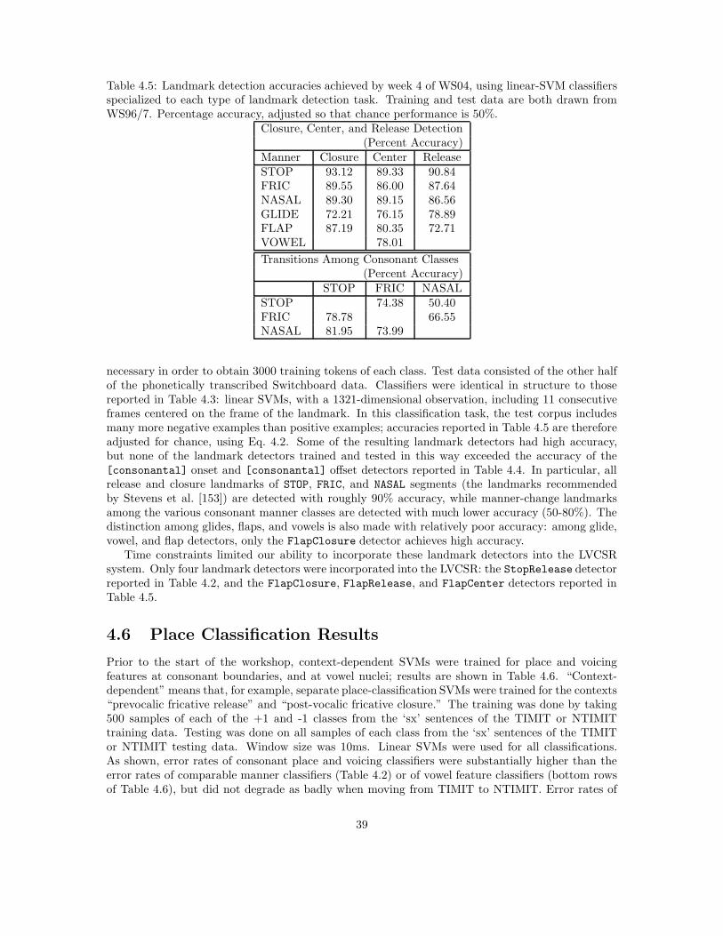
Table 4.5: Landmark detection accuracies achieved by week 4 of WS04, using linear-SVM classifiersspecialized to each type of landmark detection task. Training and test data are both drawn fromWS96/7. Percentage accuracy, adjusted so that chance performance is 50%.

Closure, Center, and Release Detection(Percent Accuracy)

Manner Closure Center ReleaseSTOP 93.12 89.33 90.84FRIC 89.55 86.00 87.64NASAL 89.30 89.15 86.56GLIDE 72.21 76.15 78.89FLAP 87.19 80.35 72.71VOWEL 78.01

Transitions Among Consonant Classes(Percent Accuracy)

STOP FRIC NASALSTOP 74.38 50.40FRIC 78.78 66.55NASAL 81.95 73.99

necessary in order to obtain 3000 training tokens of each class. Test data consisted of the other halfof the phonetically transcribed Switchboard data. Classifiers were identical in structure to thosereported in Table 4.3: linear SVMs, with a 1321-dimensional observation, including 11 consecutiveframes centered on the frame of the landmark. In this classification task, the test corpus includesmany more negative examples than positive examples; accuracies reported in Table 4.5 are thereforeadjusted for chance, using Eq. 4.2. Some of the resulting landmark detectors had high accuracy,but none of the landmark detectors trained and tested in this way exceeded the accuracy of the[consonantal] onset and [consonantal] offset detectors reported in Table 4.4. In particular, allrelease and closure landmarks of STOP, FRIC, and NASAL segments (the landmarks recommendedby Stevens et al. [153]) are detected with roughly 90% accuracy, while manner-change landmarksamong the various consonant manner classes are detected with much lower accuracy (50-80%). Thedistinction among glides, flaps, and vowels is also made with relatively poor accuracy: among glide,vowel, and flap detectors, only the FlapClosure detector achieves high accuracy.

Time constraints limited our ability to incorporate these landmark detectors into the LVCSRsystem. Only four landmark detectors were incorporated into the LVCSR: the StopRelease detectorreported in Table 4.2, and the FlapClosure, FlapRelease, and FlapCenter detectors reported inTable 4.5.

4.6 Place Classification Results

Prior to the start of the workshop, context-dependent SVMs were trained for place and voicingfeatures at consonant boundaries, and at vowel nuclei; results are shown in Table 4.6. “Context-dependent” means that, for example, separate place-classification SVMs were trained for the contexts“prevocalic fricative release” and “post-vocalic fricative closure.” The training was done by taking500 samples of each of the +1 and -1 classes from the ‘sx’ sentences of the TIMIT or NTIMITtraining data. Testing was done on all samples of each class from the ‘sx’ sentences of the TIMITor NTIMIT testing data. Window size was 10ms. Linear SVMs were used for all classifications.As shown, error rates of consonant place and voicing classifiers were substantially higher than theerror rates of comparable manner classifiers (Table 4.2) or of vowel feature classifiers (bottom rowsof Table 4.6), but did not degrade as badly when moving from TIMIT to NTIMIT. Error rates of

39

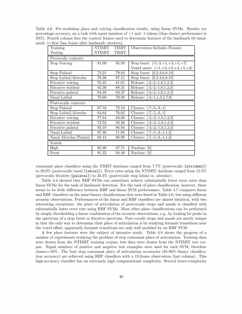
Table 4.6: Pre-workshop place and voicing classification results, using linear SVMs. Results arepercentage accuracy, on a task with equal numbers of +1 and -1 tokens (thus chance performance is50%). Fourth column lists the context frames used to determine features of the landmark (0=land-mark, 1=first 5ms frame after landmark, etcetera).

Training NTIMIT TIMIT Observation Includes Frames:Testing NTIMIT TIMIT

Prevocalic contextsStop Voicing 81.09 85.93 Stop burst: [-5,-3,+1,+3,+5,+7]

Vowel onset: [+1,+2,+3,+4,+5,+6]Stop Palatal 73.21 79.82 Stop burst: [0,2,4,6,8,10]Stop Labial/Alveolar 76.30 87.11 Stop burst: [0,2,4,6,8,10]Fricative voicing 76.35 81.01 Release: [-3,-2,-1,0,1,2,3]Fricative strident 82.30 88.31 Release: [-3,-2,-1,0,1,2,3]Fricative palatal 84.48 83.37 Release: [-3,-2,-1,0,1,2,3]Nasal Labial 78.60 79.88 Release: [-3,-1,1,3,5,7,9]

Postvocalic contextsStop Palatal 67.53 72.12 Closure: [-7,-5,-3,-1]Stop Labial/Alveolar 64.64 76.02 Closure: [-7,-5,-3,-1]Fricative voicing 77.84 83.08 Closure: [-3,-2,-1,0,1,2,3]Fricative strident 72.52 92.26 Closure: [-3,-2,-1,0,1,2,3]Fricative palatal 83.19 86.94 Closure: [-3,-2,-1,0,1,2,3]Nasal Labial 67.30 71.95 Closure: [-7,-5,-3,-1,1,3]Nasal Alveolar/Palatal 82.44 86.99 Closure: [-7,-5,-3,-1,1,3]

VowelsHigh 95.90 97.71 Nucleus: [0]Front 91.32 94.48 Nucleus: [0]

consonant place classifiers using the TIMIT database ranged from 7.7% (postvocalic [strident])to 28.0% (postvocalic nasal [labial]). Error rates using the NTIMIT database ranged from 15.5%(prevocalic fricative [palatal]) to 35.3% (postvocalic stop labial vs. alveolar).

Table 4.4 showed that RBF SVMs can sometimes achieve substantially lower error rates thanlinear SVMs for the task of landmark detection. For the task of place classification, however, thereseems to be little difference between RBF and linear SVM performance. Table 4.7 compares linearand RBF classifiers on the same binary classifications that were listed in Table 4.6, but using differentacoustic observations. Performances of the linear and RBF classifiers are almost identical, with twointeresting exceptions: the place of articulation of postvocalic stops and nasals is classified withsubstantially lower error rate using RBF SVMs. Most other place classifications can be performedby simply thresholding a linear combination of the acoustic observations, e.g., by looking for peaks inthe spectrum of a stop burst or fricative spectrum. Post-vocalic stops and nasals are nearly uniquein that the only way to determine their place of articulation is by studying formant transitions nearthe vowel offset; apparently formant transitions are only well modeled by an RBF SVM.

A few place features were the subject of intensive study. Table 4.8 shows the progress of anumber of experiments studying the problem of stop consonant place of articulation. Training datawere drawn from the NTIMIT training corpus; test data were drawn from the NTIMIT test cor-pus. Equal numbers of positive and negative test examples were used for each SVM, thereforechance=50%. The best stop consonant place of articulation accuracies (85-90% binary classifica-tion accuracy) are achieved using RBF classifiers with a 12-frame observation (last column). Thishigh-accuracy classifier has an extremely high computational complexity. Several lower-complexity

40

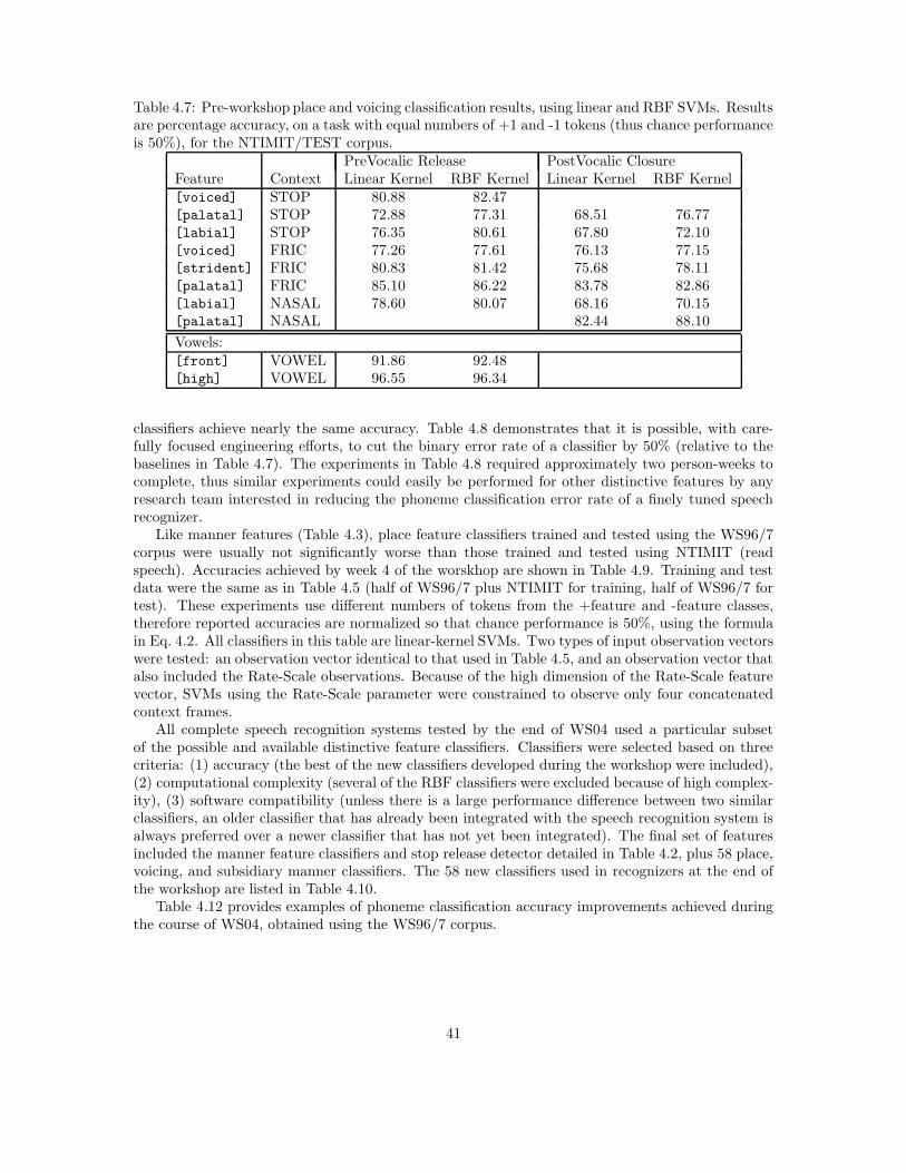
Table 4.7: Pre-workshop place and voicing classification results, using linear and RBF SVMs. Resultsare percentage accuracy, on a task with equal numbers of +1 and -1 tokens (thus chance performanceis 50%), for the NTIMIT/TEST corpus.

PreVocalic Release PostVocalic ClosureFeature Context Linear Kernel RBF Kernel Linear Kernel RBF Kernel[voiced] STOP 80.88 82.47[palatal] STOP 72.88 77.31 68.51 76.77[labial] STOP 76.35 80.61 67.80 72.10[voiced] FRIC 77.26 77.61 76.13 77.15[strident] FRIC 80.83 81.42 75.68 78.11[palatal] FRIC 85.10 86.22 83.78 82.86[labial] NASAL 78.60 80.07 68.16 70.15[palatal] NASAL 82.44 88.10

Vowels:[front] VOWEL 91.86 92.48[high] VOWEL 96.55 96.34

classifiers achieve nearly the same accuracy. Table 4.8 demonstrates that it is possible, with care-fully focused engineering efforts, to cut the binary error rate of a classifier by 50% (relative to thebaselines in Table 4.7). The experiments in Table 4.8 required approximately two person-weeks tocomplete, thus similar experiments could easily be performed for other distinctive features by anyresearch team interested in reducing the phoneme classification error rate of a finely tuned speechrecognizer.

Like manner features (Table 4.3), place feature classifiers trained and tested using the WS96/7corpus were usually not significantly worse than those trained and tested using NTIMIT (readspeech). Accuracies achieved by week 4 of the worskhop are shown in Table 4.9. Training and testdata were the same as in Table 4.5 (half of WS96/7 plus NTIMIT for training, half of WS96/7 fortest). These experiments use different numbers of tokens from the +feature and -feature classes,therefore reported accuracies are normalized so that chance performance is 50%, using the formulain Eq. 4.2. All classifiers in this table are linear-kernel SVMs. Two types of input observation vectorswere tested: an observation vector identical to that used in Table 4.5, and an observation vector thatalso included the Rate-Scale observations. Because of the high dimension of the Rate-Scale featurevector, SVMs using the Rate-Scale parameter were constrained to observe only four concatenatedcontext frames.

All complete speech recognition systems tested by the end of WS04 used a particular subsetof the possible and available distinctive feature classifiers. Classifiers were selected based on threecriteria: (1) accuracy (the best of the new classifiers developed during the workshop were included),(2) computational complexity (several of the RBF classifiers were excluded because of high complex-ity), (3) software compatibility (unless there is a large performance difference between two similarclassifiers, an older classifier that has already been integrated with the speech recognition system isalways preferred over a newer classifier that has not yet been integrated). The final set of featuresincluded the manner feature classifiers and stop release detector detailed in Table 4.2, plus 58 place,voicing, and subsidiary manner classifiers. The 58 new classifiers used in recognizers at the end ofthe workshop are listed in Table 4.10.

Table 4.12 provides examples of phoneme classification accuracy improvements achieved duringthe course of WS04, obtained using the WS96/7 corpus.

41

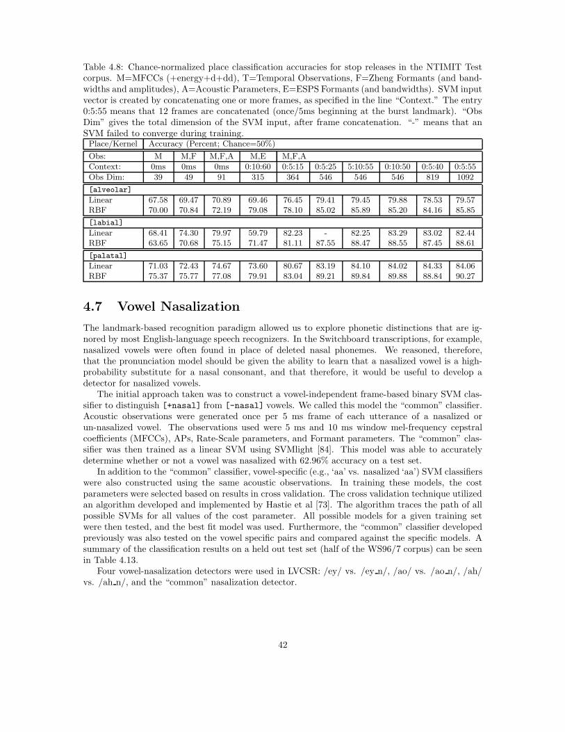
Table 4.8: Chance-normalized place classification accuracies for stop releases in the NTIMIT Testcorpus. M=MFCCs (+energy+d+dd), T=Temporal Observations, F=Zheng Formants (and band-widths and amplitudes), A=Acoustic Parameters, E=ESPS Formants (and bandwidths). SVM inputvector is created by concatenating one or more frames, as specified in the line “Context.” The entry0:5:55 means that 12 frames are concatenated (once/5ms beginning at the burst landmark). “ObsDim” gives the total dimension of the SVM input, after frame concatenation. “-” means that anSVM failed to converge during training.Place/Kernel Accuracy (Percent; Chance=50%)

Obs: M M,F M,F,A M,E M,F,A

Context: 0ms 0ms 0ms 0:10:60 0:5:15 0:5:25 5:10:55 0:10:50 0:5:40 0:5:55

Obs Dim: 39 49 91 315 364 546 546 546 819 1092

[alveolar]

Linear 67.58 69.47 70.89 69.46 76.45 79.41 79.45 79.88 78.53 79.57RBF 70.00 70.84 72.19 79.08 78.10 85.02 85.89 85.20 84.16 85.85

[labial]

Linear 68.41 74.30 79.97 59.79 82.23 - 82.25 83.29 83.02 82.44RBF 63.65 70.68 75.15 71.47 81.11 87.55 88.47 88.55 87.45 88.61

[palatal]

Linear 71.03 72.43 74.67 73.60 80.67 83.19 84.10 84.02 84.33 84.06RBF 75.37 75.77 77.08 79.91 83.04 89.21 89.84 89.88 88.84 90.27

4.7 Vowel Nasalization

The landmark-based recognition paradigm allowed us to explore phonetic distinctions that are ig-nored by most English-language speech recognizers. In the Switchboard transcriptions, for example,nasalized vowels were often found in place of deleted nasal phonemes. We reasoned, therefore,that the pronunciation model should be given the ability to learn that a nasalized vowel is a high-probability substitute for a nasal consonant, and that therefore, it would be useful to develop adetector for nasalized vowels.

The initial approach taken was to construct a vowel-independent frame-based binary SVM clas-sifier to distinguish [+nasal] from [-nasal] vowels. We called this model the “common” classifier.Acoustic observations were generated once per 5 ms frame of each utterance of a nasalized orun-nasalized vowel. The observations used were 5 ms and 10 ms window mel-frequency cepstralcoefficients (MFCCs), APs, Rate-Scale parameters, and Formant parameters. The “common” clas-sifier was then trained as a linear SVM using SVMlight [84]. This model was able to accuratelydetermine whether or not a vowel was nasalized with 62.96% accuracy on a test set.

In addition to the “common” classifier, vowel-specific (e.g., ‘aa’ vs. nasalized ‘aa’) SVM classifierswere also constructed using the same acoustic observations. In training these models, the costparameters were selected based on results in cross validation. The cross validation technique utilizedan algorithm developed and implemented by Hastie et al [73]. The algorithm traces the path of allpossible SVMs for all values of the cost parameter. All possible models for a given training setwere then tested, and the best fit model was used. Furthermore, the “common” classifier developedpreviously was also tested on the vowel specific pairs and compared against the specific models. Asummary of the classification results on a held out test set (half of the WS96/7 corpus) can be seenin Table 4.13.

Four vowel-nasalization detectors were used in LVCSR: /ey/ vs. /ey n/, /ao/ vs. /ao n/, /ah/vs. /ah n/, and the “common” nasalization detector.

42

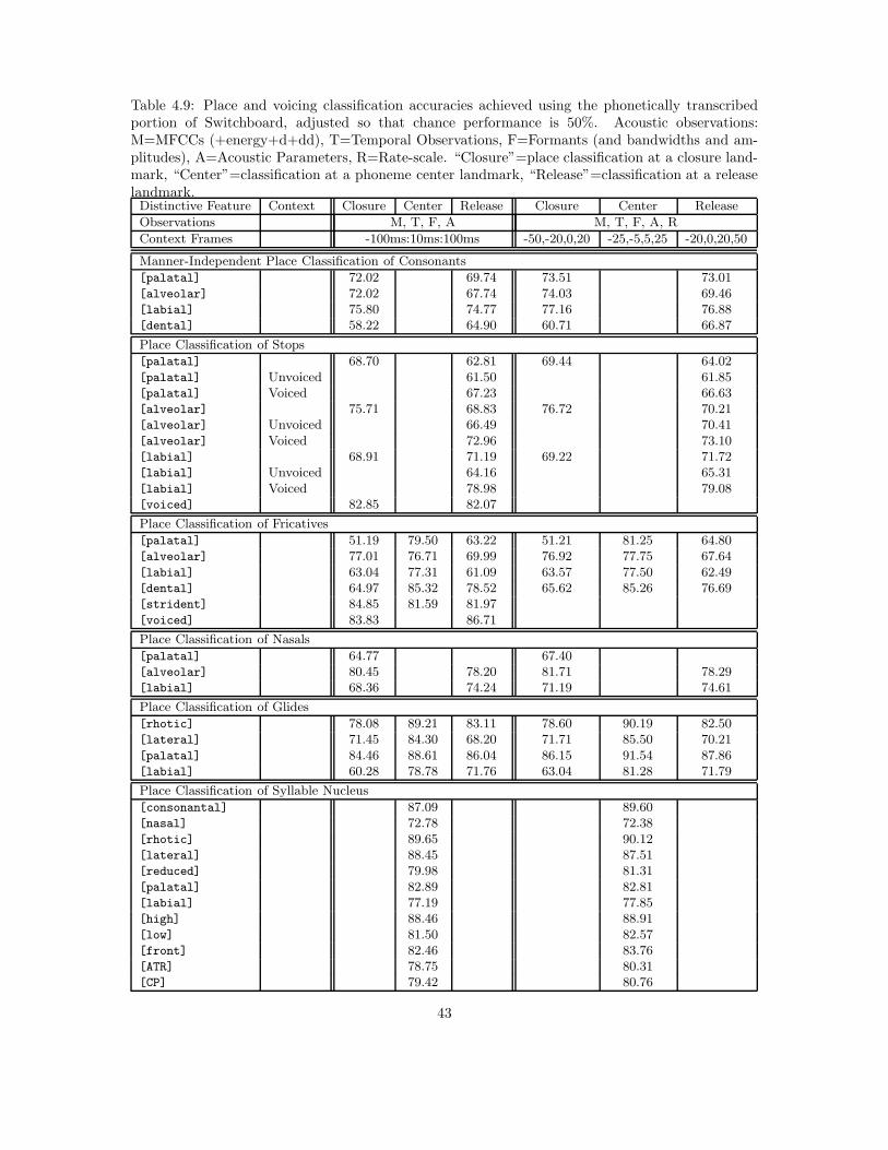
Table 4.9: Place and voicing classification accuracies achieved using the phonetically transcribedportion of Switchboard, adjusted so that chance performance is 50%. Acoustic observations:M=MFCCs (+energy+d+dd), T=Temporal Observations, F=Formants (and bandwidths and am-plitudes), A=Acoustic Parameters, R=Rate-scale. “Closure”=place classification at a closure land-mark, “Center”=classification at a phoneme center landmark, “Release”=classification at a releaselandmark.Distinctive Feature Context Closure Center Release Closure Center Release

Observations M, T, F, A M, T, F, A, R

Context Frames -100ms:10ms:100ms -50,-20,0,20 -25,-5,5,25 -20,0,20,50

Manner-Independent Place Classification of Consonants

[palatal] 72.02 69.74 73.51 73.01[alveolar] 72.02 67.74 74.03 69.46[labial] 75.80 74.77 77.16 76.88[dental] 58.22 64.90 60.71 66.87

Place Classification of Stops

[palatal] 68.70 62.81 69.44 64.02[palatal] Unvoiced 61.50 61.85[palatal] Voiced 67.23 66.63[alveolar] 75.71 68.83 76.72 70.21[alveolar] Unvoiced 66.49 70.41[alveolar] Voiced 72.96 73.10[labial] 68.91 71.19 69.22 71.72[labial] Unvoiced 64.16 65.31[labial] Voiced 78.98 79.08[voiced] 82.85 82.07

Place Classification of Fricatives

[palatal] 51.19 79.50 63.22 51.21 81.25 64.80[alveolar] 77.01 76.71 69.99 76.92 77.75 67.64[labial] 63.04 77.31 61.09 63.57 77.50 62.49[dental] 64.97 85.32 78.52 65.62 85.26 76.69[strident] 84.85 81.59 81.97[voiced] 83.83 86.71

Place Classification of Nasals

[palatal] 64.77 67.40[alveolar] 80.45 78.20 81.71 78.29[labial] 68.36 74.24 71.19 74.61

Place Classification of Glides

[rhotic] 78.08 89.21 83.11 78.60 90.19 82.50[lateral] 71.45 84.30 68.20 71.71 85.50 70.21[palatal] 84.46 88.61 86.04 86.15 91.54 87.86[labial] 60.28 78.78 71.76 63.04 81.28 71.79

Place Classification of Syllable Nucleus

[consonantal] 87.09 89.60[nasal] 72.78 72.38[rhotic] 89.65 90.12[lateral] 88.45 87.51[reduced] 79.98 81.31[palatal] 82.89 82.81[labial] 77.19 77.85[high] 88.46 88.91[low] 81.50 82.57[front] 82.46 83.76[ATR] 78.75 80.31[CP] 79.42 80.76

43

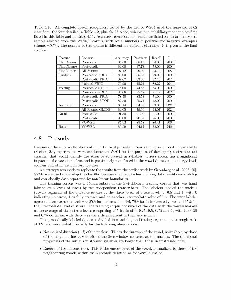
Table 4.10: All complete speech recognizers tested by the end of WS04 used the same set of 62classifiers: the four detailed in Table 4.2, plus the 58 place, voicing, and subsidiary manner classifierslisted in this table and in Table 4.11. Accuracy, precision, and recall are listed for an arbitrary testsample selected from the WS96/7 corpus, with equal numbers of positive and negative examples(chance=50%). The number of test tokens is different for different classifiers; N is given in the finalcolumn.

Feature Context Accuracy Precision Recall N

FlapRelease Prevocalic 85.50 85.15 86.00 200

FlapClosure Postvocalic 84.00 87.78 79.00 200

FlapCenter All Frames 97.12 99.00 95.19 208

Strident Prevocalic FRIC 83.00 85.87 79.00 200

Postvocalic FRIC 82.67 83.00 82.18 202

Isolated FRIC 79.90 75.21 89.22 204

Voicing Prevocalic STOP 78.00 74.56 85.00 200

Prevocalic FRIC 83.66 85.42 81.19 202

Postvocalic FRIC 78.50 83.53 71.00 200

Postvocalic STOP 82.50 85.71 78.00 200

Aspiration Prevocalic 66.14 64.99 69.98 1326

All Frames GLIDE 84.65 79.66 93.07 202

Nasal Prevocalic 91.50 91.92 91.00 200

Postvocalic 93.00 90.57 96.00 200

VOWEL 85.92 85.58 86.41 206

Body VOWEL 86.59 94.12 78.05 246

4.8 Prosody

Because of the empirically observed importance of prosody in constraining pronunciation variability(Section 2.4, experiments were conducted at WS04 for the purpose of developing a stress-accentclassifier that would identify the stress level present in syllables. Stress accent has a significantimpact on the vocalic nucleus and is particularly manifested in the vowel duration, its energy level,contour and other articulatory features.

An attempt was made to replicate the results from the earlier work by Greenberg et al. 2003 [60].SVMs were used to develop the classifier because they require less training data, avoid over trainingand can classify data separated by non-linear boundaries.

The training corpus was a 45-min subset of the Switchboard training corpus that was handlabeled at 3 levels of stress by two independent transcribers. The labelers labeled the nucleus(vowel) segments of the syllables as one of the three levels of stress level: 0, 0.5 and 1, with 0indicating no stress, 1 as fully stressed and an another intermediate value of 0.5. The inter-labeleragreement on stressed vowels was 85% for unstressed nuclei, 78% for fully stressed vowel and 95% forthe intermediate level of stress. The training corpus consisted of the data with the vowels markedas the average of their stress levels comprising of 5 levels of 0, 0.25, 0.5, 0.75 and 1, with the 0.25and 0.75 occurring with there was the a disagreement in their assessment.

This prosodically labeled data was divided into training and testing segments, at a rough ratioof 3:2, and were tested primarily for the following observations:

• Normalized duration (nd) of the nucleus. This is the duration of the vowel, normalized by thoseof the neighbouring vowels within the 3sec window centered at the nucleus. The durationalproperties of the nucleus in stressed syllables are longer than those in unstressed ones.

• Energy of the nucleus (ne). This is the energy level of the vowel, normalized to those of theneighbouring vowels within the 3 seconds duration as for vowel duration

44

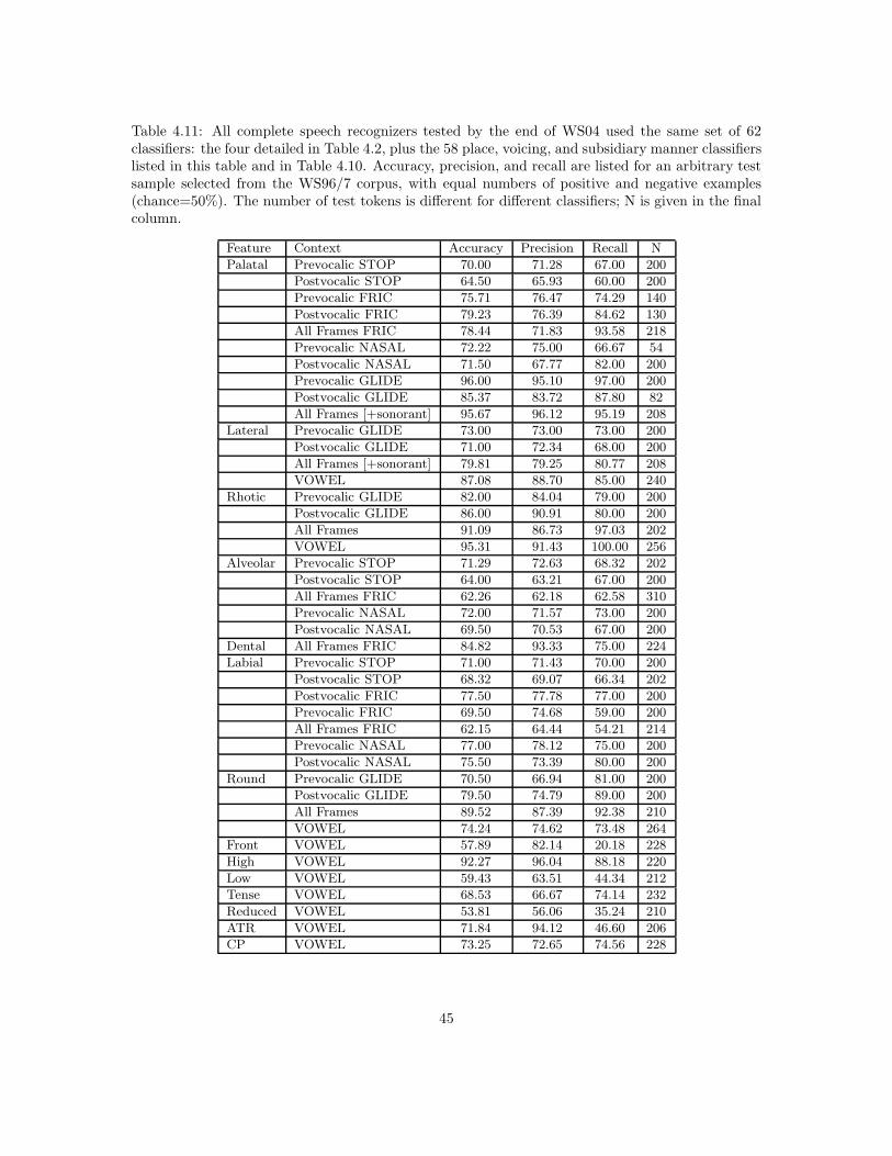
Table 4.11: All complete speech recognizers tested by the end of WS04 used the same set of 62classifiers: the four detailed in Table 4.2, plus the 58 place, voicing, and subsidiary manner classifierslisted in this table and in Table 4.10. Accuracy, precision, and recall are listed for an arbitrary testsample selected from the WS96/7 corpus, with equal numbers of positive and negative examples(chance=50%). The number of test tokens is different for different classifiers; N is given in the finalcolumn.

Feature Context Accuracy Precision Recall N

Palatal Prevocalic STOP 70.00 71.28 67.00 200

Postvocalic STOP 64.50 65.93 60.00 200

Prevocalic FRIC 75.71 76.47 74.29 140

Postvocalic FRIC 79.23 76.39 84.62 130

All Frames FRIC 78.44 71.83 93.58 218

Prevocalic NASAL 72.22 75.00 66.67 54

Postvocalic NASAL 71.50 67.77 82.00 200

Prevocalic GLIDE 96.00 95.10 97.00 200

Postvocalic GLIDE 85.37 83.72 87.80 82

All Frames [+sonorant] 95.67 96.12 95.19 208

Lateral Prevocalic GLIDE 73.00 73.00 73.00 200

Postvocalic GLIDE 71.00 72.34 68.00 200

All Frames [+sonorant] 79.81 79.25 80.77 208

VOWEL 87.08 88.70 85.00 240

Rhotic Prevocalic GLIDE 82.00 84.04 79.00 200

Postvocalic GLIDE 86.00 90.91 80.00 200

All Frames 91.09 86.73 97.03 202

VOWEL 95.31 91.43 100.00 256

Alveolar Prevocalic STOP 71.29 72.63 68.32 202

Postvocalic STOP 64.00 63.21 67.00 200

All Frames FRIC 62.26 62.18 62.58 310

Prevocalic NASAL 72.00 71.57 73.00 200

Postvocalic NASAL 69.50 70.53 67.00 200

Dental All Frames FRIC 84.82 93.33 75.00 224

Labial Prevocalic STOP 71.00 71.43 70.00 200

Postvocalic STOP 68.32 69.07 66.34 202

Postvocalic FRIC 77.50 77.78 77.00 200

Prevocalic FRIC 69.50 74.68 59.00 200

All Frames FRIC 62.15 64.44 54.21 214

Prevocalic NASAL 77.00 78.12 75.00 200

Postvocalic NASAL 75.50 73.39 80.00 200

Round Prevocalic GLIDE 70.50 66.94 81.00 200

Postvocalic GLIDE 79.50 74.79 89.00 200

All Frames 89.52 87.39 92.38 210

VOWEL 74.24 74.62 73.48 264

Front VOWEL 57.89 82.14 20.18 228

High VOWEL 92.27 96.04 88.18 220

Low VOWEL 59.43 63.51 44.34 212

Tense VOWEL 68.53 66.67 74.14 232

Reduced VOWEL 53.81 56.06 35.24 210

ATR VOWEL 71.84 94.12 46.60 206

CP VOWEL 73.25 72.65 74.56 228

45

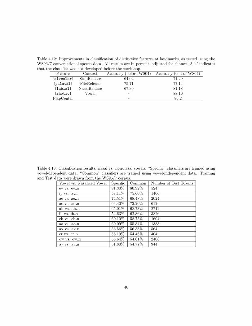
Table 4.12: Improvements in classification of distinctive features at landmarks, as tested using theWS96/7 conversational speech data. All results are in percent, adjusted for chance. A ’-’ indicatesthat the classifier was not developed before the workshop.

Feature Context Accuracy (before WS04) Accuracy (end of WS04)[alveolar] StopRelease 64.02 71.29[palatal] FricRelease 75.71 77.14[labial] NasalRelease 67.30 81.18[rhotic] Vowel - 88.16

FlapCenter - 86.2

Table 4.13: Classification results: nasal vs. non-nasal vowels. “Specific” classifiers are trained usingvowel-dependent data; “Common” classifiers are trained using vowel-independent data. Trainingand Test data were drawn from the WS96/7 corpus.

Vowel vs. Nasalized Vowel Specific Common Number of Test Tokensey vs. ey n 81.30% 80.92% 524iy vs. iy n 58.11% 75.60% 1406ae vs. ae n 74.51% 68.48% 2024ao vs. ao n 63.40% 73.20% 612ah vs. ah n 65.01% 68.73% 2712ih vs. ih n 54.63% 62.36% 3826eh vs. eh n 60.10% 58.73% 1604aa vs. aa n 60.09% 55.84% 1388ax vs. ax n 56.56% 56.38% 564er vs. er n 56.19% 54.46% 404ow vs. ow n 55.64% 54.61% 2408ay vs. ay n 51.80% 54.77% 944

46

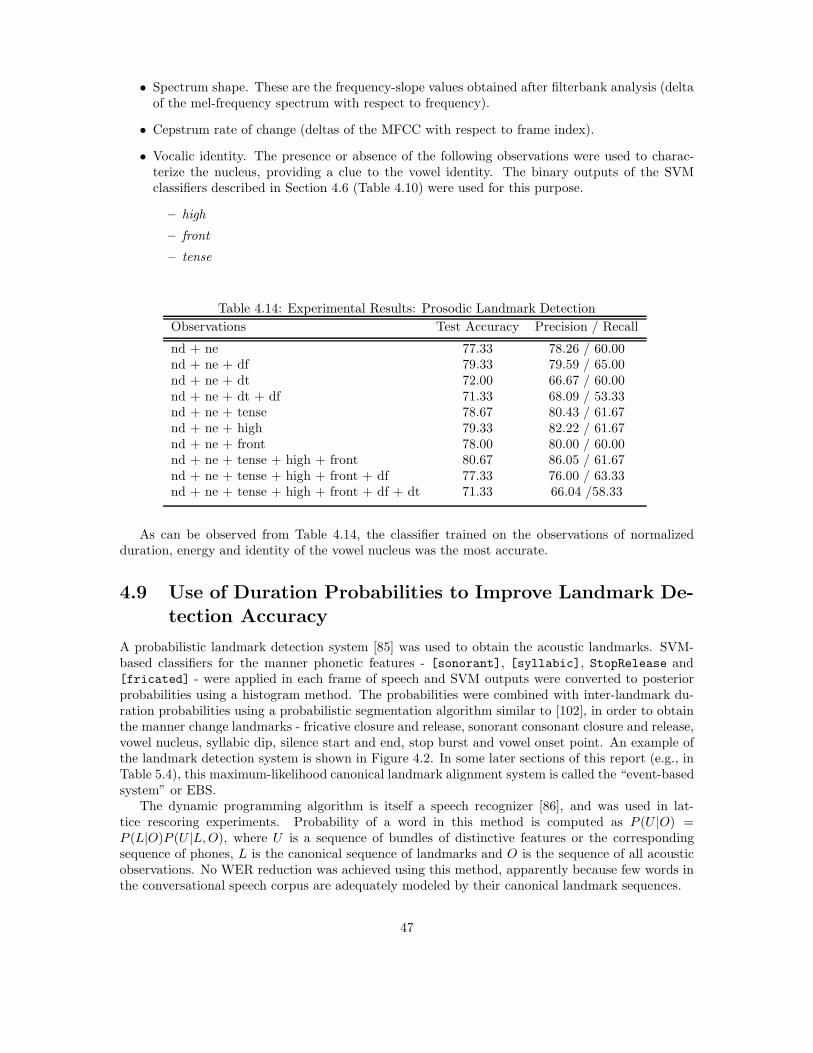
• Spectrum shape. These are the frequency-slope values obtained after filterbank analysis (deltaof the mel-frequency spectrum with respect to frequency).

• Cepstrum rate of change (deltas of the MFCC with respect to frame index).

• Vocalic identity. The presence or absence of the following observations were used to charac-terize the nucleus, providing a clue to the vowel identity. The binary outputs of the SVMclassifiers described in Section 4.6 (Table 4.10) were used for this purpose.

– high

– front

– tense

Table 4.14: Experimental Results: Prosodic Landmark Detection

Observations Test Accuracy Precision / Recall

nd + ne 77.33 78.26 / 60.00nd + ne + df 79.33 79.59 / 65.00nd + ne + dt 72.00 66.67 / 60.00nd + ne + dt + df 71.33 68.09 / 53.33nd + ne + tense 78.67 80.43 / 61.67nd + ne + high 79.33 82.22 / 61.67nd + ne + front 78.00 80.00 / 60.00nd + ne + tense + high + front 80.67 86.05 / 61.67nd + ne + tense + high + front + df 77.33 76.00 / 63.33nd + ne + tense + high + front + df + dt 71.33 66.04 /58.33

As can be observed from Table 4.14, the classifier trained on the observations of normalizedduration, energy and identity of the vowel nucleus was the most accurate.

4.9 Use of Duration Probabilities to Improve Landmark De-

tection Accuracy

A probabilistic landmark detection system [85] was used to obtain the acoustic landmarks. SVM-based classifiers for the manner phonetic features - [sonorant], [syllabic], StopRelease and[fricated] - were applied in each frame of speech and SVM outputs were converted to posteriorprobabilities using a histogram method. The probabilities were combined with inter-landmark du-ration probabilities using a probabilistic segmentation algorithm similar to [102], in order to obtainthe manner change landmarks - fricative closure and release, sonorant consonant closure and release,vowel nucleus, syllabic dip, silence start and end, stop burst and vowel onset point. An example ofthe landmark detection system is shown in Figure 4.2. In some later sections of this report (e.g., inTable 5.4), this maximum-likelihood canonical landmark alignment system is called the “event-basedsystem” or EBS.

The dynamic programming algorithm is itself a speech recognizer [86], and was used in lat-tice rescoring experiments. Probability of a word in this method is computed as P (U |O) =P (L|O)P (U |L, O), where U is a sequence of bundles of distinctive features or the correspondingsequence of phones, L is the canonical sequence of landmarks and O is the sequence of all acousticobservations. No WER reduction was achieved using this method, apparently because few words inthe conversational speech corpus are adequately modeled by their canonical landmark sequences.

47

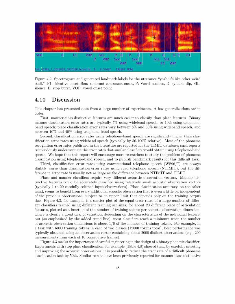
Figure 4.2: Spectrogram and generated landmark labels for the utterance “yeah it’s like other weirdstuff.” F1: fricative onset, Son: sonorant consonant onset, P: Vowel nucleus, D: syllabic dip, SIL:silence, B: stop burst, VOP: vowel onset point

4.10 Discussion

This chapter has presented data from a large number of experiments. A few generalizations are inorder.

First, manner-class distinctive features are much easier to classify than place features. Binarymanner classification error rates are typically 5% using wideband speech, or 10% using telephone-band speech; place classification error rates vary between 8% and 30% using wideband speech, andbetween 10% and 40% using telephone-band speech.

Second, classification error rates using telephone-band speech are significantly higher than clas-sification error rates using wideband speech (typically by 50-100% relative). Most of the phonemerecognition error rates published in the literature are reported for the TIMIT database; such reportstremendously underestimate the error rates that similar classifiers would obtain using telephone-bandspeech. We hope that this report will encourage more researchers to study the problem of phonemeclassification using telephone-band speech, and to publish benchmark results for this difficult task.

Third, classification error rates using conversational telephone speech (WS96/7) are alwaysslightly worse than classification error rates using read telephone speech (NTIMIT), but the dif-ference in error rate is usually not as large as the difference between NTIMIT and TIMIT.

Place and manner classifiers require very different acoustic observation vectors. Manner dis-tinctive features could be accurately classified using relatively small acoustic observation vectors(typically 1 to 20 carefully selected input observations). Place classification accuracy, on the otherhand, seems to benefit from every additional acoustic observation that is even a little bit independentof the previous observations, subject to an upper limit that depends only on the training corpussize. Figure 4.3, for example, is a scatter plot of the equal error rates of a large number of differ-ent classifiers trained using different training set sizes, for about 20 different place of articulationfeatures, plotted as a function of the number of training tokens per acoustic observation dimension.There is clearly a great deal of variation, depending on the characteristics of the individual feature,but (as emphasized by the added trend line), most classifiers reach a minimum when the numberof acoustic observation dimensions is about 1/6 of the number of training tokens. For example, ina task with 6000 training tokens in each of two classes (12000 tokens total), best performance wastypically obtained using an observation vector containing about 2000 distinct observations (e.g., 200measurements from each of 10 consecutive frames).

Figure 4.3 masks the importance of careful engineering in the design of a binary phonetic classifier.Experiments with stop place classification, for example (Table 4.8) showed that, by carefully selectingand improving the acoustic observations, it is possible to reduce the error rate of a difficult phonemeclassification task by 50%. Similar results have been previously reported for manner-class distinctive

48

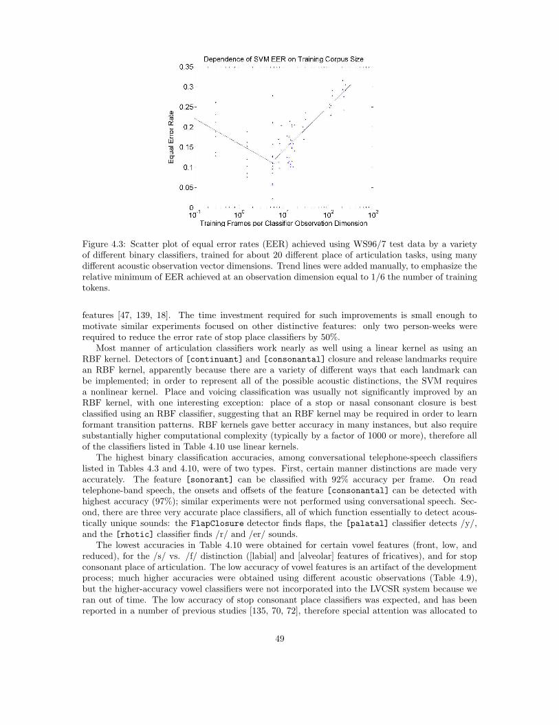
Figure 4.3: Scatter plot of equal error rates (EER) achieved using WS96/7 test data by a varietyof different binary classifiers, trained for about 20 different place of articulation tasks, using manydifferent acoustic observation vector dimensions. Trend lines were added manually, to emphasize therelative minimum of EER achieved at an observation dimension equal to 1/6 the number of trainingtokens.

features [47, 139, 18]. The time investment required for such improvements is small enough tomotivate similar experiments focused on other distinctive features: only two person-weeks wererequired to reduce the error rate of stop place classifiers by 50%.

Most manner of articulation classifiers work nearly as well using a linear kernel as using anRBF kernel. Detectors of [continuant] and [consonantal] closure and release landmarks requirean RBF kernel, apparently because there are a variety of different ways that each landmark canbe implemented; in order to represent all of the possible acoustic distinctions, the SVM requiresa nonlinear kernel. Place and voicing classification was usually not significantly improved by anRBF kernel, with one interesting exception: place of a stop or nasal consonant closure is bestclassified using an RBF classifier, suggesting that an RBF kernel may be required in order to learnformant transition patterns. RBF kernels gave better accuracy in many instances, but also requiresubstantially higher computational complexity (typically by a factor of 1000 or more), therefore allof the classifiers listed in Table 4.10 use linear kernels.

The highest binary classification accuracies, among conversational telephone-speech classifierslisted in Tables 4.3 and 4.10, were of two types. First, certain manner distinctions are made veryaccurately. The feature [sonorant] can be classified with 92% accuracy per frame. On readtelephone-band speech, the onsets and offsets of the feature [consonantal] can be detected withhighest accuracy (97%); similar experiments were not performed using conversational speech. Sec-ond, there are three very accurate place classifiers, all of which function essentially to detect acous-tically unique sounds: the FlapClosure detector finds flaps, the [palatal] classifier detects /y/,and the [rhotic] classifier finds /r/ and /er/ sounds.

The lowest accuracies in Table 4.10 were obtained for certain vowel features (front, low, andreduced), for the /s/ vs. /f/ distinction ([labial] and [alveolar] features of fricatives), and for stopconsonant place of articulation. The low accuracy of vowel features is an artifact of the developmentprocess; much higher accuracies were obtained using different acoustic observations (Table 4.9),but the higher-accuracy vowel classifiers were not incorporated into the LVCSR system because weran out of time. The low accuracy of stop consonant place classifiers was expected, and has beenreported in a number of previous studies [135, 70, 72], therefore special attention was allocated to

49

the improvement of pre-vocalic stop place classification. From an accuracy of about 64% at thestart of the workshop, binary alveolar vs. non-alveolar place classification improved to about 72%by the end of the workshop (using a linear kernel; using an RBF kernel, accuracies of about 90%could be achieved). Similar attention should be paid, in future experiments, to place classificationof post-vocalic stops.

50

Chapter 5

Rescoring Using a Generative

Feature-Based Pronunciation

Model

Once the probabilities of distinctive features and landmarks have been computed using the SVMs,a model is needed to combine the probabilities into word or utterance scores. One approach thatwe studied as part of the workshop was a generative model, that is, a model that generates theprobability of a given set of feature values given a specified word or utterance. We refer to such amodel as a feature-based pronunciation model.

One issue we try to address with this model is that the surface feature values and landmarklocations may not neatly correspond to phonetic segments. Different features may evolve at differentrates and may not reach their target values, resulting in segments of speech that do not correspondto any phone in the English phonetic inventory and in which boundaries between segments are notclearly defined. Furthermore, even in cases where we could conceive of representing the surfacepronunciations using some expanded phonetic inventory, it may be more parsimonious to describethe phenomena in terms of the articulatory processes that cause them. In order to illustrate this,we consider several examples of pronunciation variation 1.

One common phenomenon is the nasalization of vowels preceding nasal consonants. This is aresult of asynchrony: The velum is lowered before the oral closure is made. In extreme cases, thenasal consonant is entirely absent, leaving only a nasalized vowel, as in can’t → [ k ae n t ] 2. All ofthe underlying feature trajectories are correct, although phonetically, this would be described as adeletion.

Another example, taken from the phonetically-transcribed portion of the Switchboard corpus [63],is several → [s eh r v ax l]. In this case, the tongue and lips have desynchronized to the point thatthe tongue retroflexion for [r] starts before the lip narrowing for [v]. Again, all of the articulatorytrajectories are correct, but there is an apparent exchange of two phones, which cannot be representedvia single-phone confusions conditioned on phonemic context.

A final example from Switchboard is everybody → [eh r uw ay]. It is difficult to imagine a set of(reasonable) phonetic transformations that would predict this pronunciation. However, when viewedin terms of speech production, the transformation from [eh v r iy bcl b ah dx iy] to [eh r uw ay] isnot too complicated. The tongue and lips desynchronize, with the lips starting to close for the [bcl]quite early during the previous vowel. In addition, the lip constrictions for [bcl] and [v], and the

1These examples, as well as parts of Section 5.1, are taken from [107].2Here and throughout this section, we use the ARPAbet phonetic symbol set with additional diacritics, such as

“ n” for nasalization.

51

tongue tip gesture for [dx], are reduced to sonorants.The general theme that emerges from examining these kinds of examples, and the assumption

that we will make, is that a great deal of pronunciation variation can be described using a limitedamount of (i) asynchrony between features and (ii) reductions from the target feature values tovalues that are more “neutral” or else more similar to neighboring feature values. Another themethat these examples share is that it seems natural to describe them in terms of speech productionprocesses, that is, in terms of the trajectories of the articulators. On the other hand, for reasonsdiscussed in previous sections, the acoustic analysis is done in terms of binary distinctive features,rather than articulatory features. In this part of the project, we investigated the possibility of usingdifferent feature sets for the pronunciation model and acoustic model, allowing each part of therecognizer to use the representation best suited to its task.

5.1 From Words to Landmarks and Distinctive Features

The generative pronunciation model used at the workshop is based on the one described in [107, 108].The feature set in this model is an articulatory one and is based on the “vocal tract variables” ofarticulatory phonology [24]. The features consist of the locations and/or degrees of opening of thelips, tongue tip, and tongue body, and the states of the glottis and velum; see Appendix A.2. Themodel generates, for a given word, all possible pronunciations of the word and their probabilities,where a “pronunciation” consists of all of the articulatory feature (AF) values in each frame.

Section 5.1.1 describes this pronunciation model. Section 5.1.2 describes how this model iscombined with the SVM classifier outputs to produce word scores.

5.1.1 The Production-Based Pronunciation Model

The pronunciation model begins with the usual assumption that each word has one or more targetphonemic pronunciations, or baseforms. Each baseform is converted to a matrix of underlying featurevalues via a phone-to-feature mapping table; see Appendix A.3 for the mapping table used at theworkshop. Table 5.1 shows what a part of this matrix might look like for the phrase I don’t know.The matrix may include ‘unspecified’ values (‘*’ in the table). More generally, each matrix entrycan be a distribution over the range of feature values. For now, we assume that all of the features gothrough the same sequence of indices (and therefore the same number of targets) in a given word;e.g., in Table 5.1, LIP-OPEN goes through the same indices as TT-OPEN, although it has fewerdistinct target values. This assumption makes it easy to model asynchrony by referring to featureindices, as well as enforcing a minimum duration constraint.

The actual (surface) feature values can stray from the target pronunciation in two ways: substi-tution, in which a feature’s surface value at a given time differs from its underlying value, typicallybecause of articulatory inertia; and asynchrony, in which different features proceed through theirsequences of values at different rates. The degree of asynchrony is not completely free: We assumethat it has an upper bound, and within this bound, different levels of asynchrony have different prob-abilities (or costs). The synchronization requirements are expressed as constraints on the averageindex of one subset of the features relative to the average index of another subset.

Dynamic Bayesian networks provide a natural framework for such a model, because of theirability to efficiently implement factored state representations. The dashed box in Figure 5.1 showsone frame of the type of DBN used in our model (simplified somewhat for clarity of presentation).This example DBN assumes a feature set with three features. The variables at time frame t, andtheir associated conditional distributions, are as follows:

wordt – the current word. This simplified graph assumes one pronunciation per word; in practice,we allowed several pronunciations per word by having an additional variable representing thepronunciation variant.

52

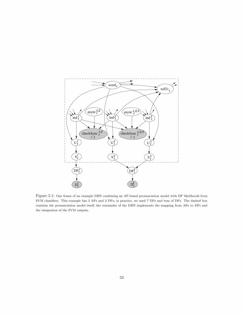
tasync1;2

t1,2;3

= 1checkSync

t1,2;3async

S1 2 3S St t

DF1 DF2

1D D2

2 3

U UU

ind ind ind

1 2 3

t t

tt

1t

t

twdTrword t

= 1t1;2checkSync

t

tt

t t

Figure 5.1: One frame of an example DBN combining an AF-based pronunciation model with DF likelihoods from

SVM classifiers. This example has 3 AFs and 2 DFs; in practice, we used 7 DFs and tens of DFs. The dashed box

contains the pronunciation model itself; the remainder of the DBN implements the mapping from AFs to DFs and

the integration of the SVM outputs.

53

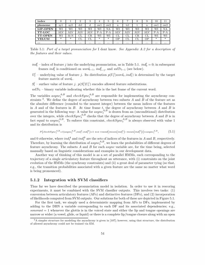
index 0 1 2 3 4 5 6 7 8 9 10 11

phoneme ay1 ay2 dcl d ow1 ow2 n tcl t n ow1 ow2

LIP-OPEN WI WI WI WI WI NA WI WI WI WI WI NATT-LOC ALV ALV ALV ALV P-A P-A ALV ALV ALV ALV P-A P-ATT-OPEN WI M-N CL CR WI WI CL CL CR CL WI WIVELUM * * CL CL * * OP CL CL OP * *... ... ... ... ... ... ... ... ... ... ... ... ...

Table 5.1: Part of a target pronunciation for I dont know. See Appendix A.2 for a description ofthe features and their values.

indjt – index of feature j into the underlying pronunciation, as in Table 5.1. indj

0 = 0; in subsequent

frames indjt is conditioned on wordt−1, indj

t−1, and wdTrt−1 (see below).

Ujt – underlying value of feature j. Its distribution p(U j

t |wordt, indjt ) is determined by the target

feature matrix of wordt.

Sjt – surface value of feature j. p(Sj

t |Ujt ) encodes allowed feature substitutions.

wdTrt – binary variable indicating whether this is the last frame of the current word.

The variables asyncA;Bt and checkSyncA;B

t are responsible for implementing the asynchrony con-straints 3. We define the degree of asynchrony between two subsets A and B of the feature set asthe absolute difference (rounded to the nearest integer) between the mean indices of the featuresin A and of the features in B. At time frame t, the degree of asynchrony between A and B isgenerated in the following way: A value for asyncA;B

t is drawn from an (unconditional) distribution

over the integers, while checkSyncA;Bt checks that the degree of asynchrony between A and B is in

fact equal to asyncA;Bt . To enforce this constraint, checkSyncA;B

t is always observed with value 1and its distribution is

P(checkSyncA;Bt

=1|asyncA;Bt

,indA

t,indB

t )=1 ⇐⇒ round(|mean(indA

t )−mean(indB

t )|)=asyncA;Bt

, (5.1)

and 0 otherwise, where indAt and indB

t are the sets of indices of the features in A and B, respectively.

Therefore, by learning the distribution of asyncA;Bt , we learn the probabilities of different degrees of

feature asynchrony. The subsets A and B for each async variable are, for the time being, selectedmanually based on linguistic considerations and examples in our development data.

Another way of thinking of this model is as a set of parallel HMMs, each corresponding to thetrajectory of a single articulatory feature throughout an utterance, with (i) constraints on the jointevolution of the HMMs (the synchrony constraints) and (ii) a great deal of parameter tying (so that,e.g., the transition probabilities associated with a given feature are the same no matter what wordis being pronounced).

5.1.2 Integration with SVM classifiers

Thus far we have described the pronunciation model in isolation. In order to use it in rescoringexperiments, it must be combined with the SVM classifier outputs. This involves two tasks: (1)conversion between articulatory features (AFs) and distinctive features (DFs), and (2) incorporationof likelihoods computed from SVM outputs. Our solutions for both of these are depicted in Figure 5.1.

For the first task, we simply used a deterministic mapping from AFs to DFs, implemented byadding to the DBN a variable corresponding to each DF and its associated dependencies; e.g.,sonorant = 1 whenever the glottis is in the voiced state and either the lip and tongue openings arenarrow or wider (a vowel, glide, or liquid) or there is a complete lip/tongue closure along with an open

3A simpler structure for modeling the asynchrony is given in [107]; however, using that structure, the distributionof allowed asynchrony could not be trained via EM.

54

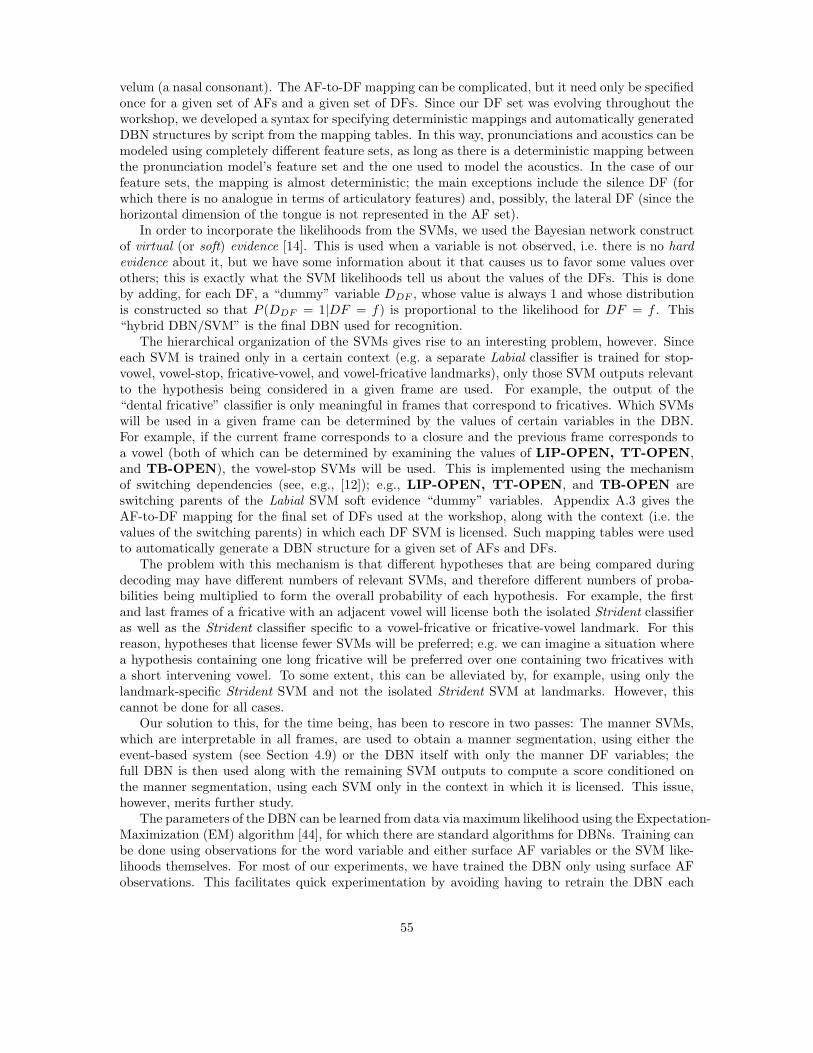
velum (a nasal consonant). The AF-to-DF mapping can be complicated, but it need only be specifiedonce for a given set of AFs and a given set of DFs. Since our DF set was evolving throughout theworkshop, we developed a syntax for specifying deterministic mappings and automatically generatedDBN structures by script from the mapping tables. In this way, pronunciations and acoustics can bemodeled using completely different feature sets, as long as there is a deterministic mapping betweenthe pronunciation model’s feature set and the one used to model the acoustics. In the case of ourfeature sets, the mapping is almost deterministic; the main exceptions include the silence DF (forwhich there is no analogue in terms of articulatory features) and, possibly, the lateral DF (since thehorizontal dimension of the tongue is not represented in the AF set).

In order to incorporate the likelihoods from the SVMs, we used the Bayesian network constructof virtual (or soft) evidence [14]. This is used when a variable is not observed, i.e. there is no hardevidence about it, but we have some information about it that causes us to favor some values overothers; this is exactly what the SVM likelihoods tell us about the values of the DFs. This is doneby adding, for each DF, a “dummy” variable DDF , whose value is always 1 and whose distributionis constructed so that P (DDF = 1|DF = f) is proportional to the likelihood for DF = f . This“hybrid DBN/SVM” is the final DBN used for recognition.

The hierarchical organization of the SVMs gives rise to an interesting problem, however. Sinceeach SVM is trained only in a certain context (e.g. a separate Labial classifier is trained for stop-vowel, vowel-stop, fricative-vowel, and vowel-fricative landmarks), only those SVM outputs relevantto the hypothesis being considered in a given frame are used. For example, the output of the“dental fricative” classifier is only meaningful in frames that correspond to fricatives. Which SVMswill be used in a given frame can be determined by the values of certain variables in the DBN.For example, if the current frame corresponds to a closure and the previous frame corresponds toa vowel (both of which can be determined by examining the values of LIP-OPEN, TT-OPEN,and TB-OPEN), the vowel-stop SVMs will be used. This is implemented using the mechanismof switching dependencies (see, e.g., [12]); e.g., LIP-OPEN, TT-OPEN, and TB-OPEN areswitching parents of the Labial SVM soft evidence “dummy” variables. Appendix A.3 gives theAF-to-DF mapping for the final set of DFs used at the workshop, along with the context (i.e. thevalues of the switching parents) in which each DF SVM is licensed. Such mapping tables were usedto automatically generate a DBN structure for a given set of AFs and DFs.

The problem with this mechanism is that different hypotheses that are being compared duringdecoding may have different numbers of relevant SVMs, and therefore different numbers of proba-bilities being multiplied to form the overall probability of each hypothesis. For example, the firstand last frames of a fricative with an adjacent vowel will license both the isolated Strident classifieras well as the Strident classifier specific to a vowel-fricative or fricative-vowel landmark. For thisreason, hypotheses that license fewer SVMs will be preferred; e.g. we can imagine a situation wherea hypothesis containing one long fricative will be preferred over one containing two fricatives witha short intervening vowel. To some extent, this can be alleviated by, for example, using only thelandmark-specific Strident SVM and not the isolated Strident SVM at landmarks. However, thiscannot be done for all cases.

Our solution to this, for the time being, has been to rescore in two passes: The manner SVMs,which are interpretable in all frames, are used to obtain a manner segmentation, using either theevent-based system (see Section 4.9) or the DBN itself with only the manner DF variables; thefull DBN is then used along with the remaining SVM outputs to compute a score conditioned onthe manner segmentation, using each SVM only in the context in which it is licensed. This issue,however, merits further study.

The parameters of the DBN can be learned from data via maximum likelihood using the Expectation-Maximization (EM) algorithm [44], for which there are standard algorithms for DBNs. Training canbe done using observations for the word variable and either surface AF variables or the SVM like-lihoods themselves. For most of our experiments, we have trained the DBN only using surface AFobservations. This facilitates quick experimentation by avoiding having to retrain the DBN each

55

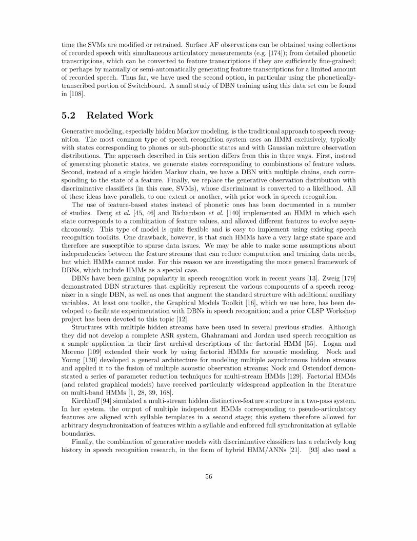
time the SVMs are modified or retrained. Surface AF observations can be obtained using collectionsof recorded speech with simultaneous articulatory measurements (e.g. [174]); from detailed phonetictranscriptions, which can be converted to feature transcriptions if they are sufficiently fine-grained;or perhaps by manually or semi-automatically generating feature transcriptions for a limited amountof recorded speech. Thus far, we have used the second option, in particular using the phonetically-transcribed portion of Switchboard. A small study of DBN training using this data set can be foundin [108].

5.2 Related Work

Generative modeling, especially hidden Markov modeling, is the traditional approach to speech recog-nition. The most common type of speech recognition system uses an HMM exclusively, typicallywith states corresponding to phones or sub-phonetic states and with Gaussian mixture observationdistributions. The approach described in this section differs from this in three ways. First, insteadof generating phonetic states, we generate states corresponding to combinations of feature values.Second, instead of a single hidden Markov chain, we have a DBN with multiple chains, each corre-sponding to the state of a feature. Finally, we replace the generative observation distribution withdiscriminative classifiers (in this case, SVMs), whose discriminant is converted to a likelihood. Allof these ideas have parallels, to one extent or another, with prior work in speech recognition.

The use of feature-based states instead of phonetic ones has been documented in a numberof studies. Deng et al. [45, 46] and Richardson et al. [140] implemented an HMM in which eachstate corresponds to a combination of feature values, and allowed different features to evolve asyn-chronously. This type of model is quite flexible and is easy to implement using existing speechrecognition toolkits. One drawback, however, is that such HMMs have a very large state space andtherefore are susceptible to sparse data issues. We may be able to make some assumptions aboutindependencies between the feature streams that can reduce computation and training data needs,but which HMMs cannot make. For this reason we are investigating the more general framework ofDBNs, which include HMMs as a special case.

DBNs have been gaining popularity in speech recognition work in recent years [13]. Zweig [179]demonstrated DBN structures that explicitly represent the various components of a speech recog-nizer in a single DBN, as well as ones that augment the standard structure with additional auxiliaryvariables. At least one toolkit, the Graphical Models Toolkit [16], which we use here, has been de-veloped to facilitate experimentation with DBNs in speech recognition; and a prior CLSP Workshopproject has been devoted to this topic [12].

Structures with multiple hidden streams have been used in several previous studies. Althoughthey did not develop a complete ASR system, Ghahramani and Jordan used speech recognition asa sample application in their first archival descriptions of the factorial HMM [55]. Logan andMoreno [109] extended their work by using factorial HMMs for acoustic modeling. Nock andYoung [130] developed a general architecture for modeling multiple asynchronous hidden streamsand applied it to the fusion of multiple acoustic observation streams; Nock and Ostendorf demon-strated a series of parameter reduction techniques for multi-stream HMMs [129]. Factorial HMMs(and related graphical models) have received particularly widespread application in the literatureon multi-band HMMs [1, 28, 39, 168].

Kirchhoff [94] simulated a multi-stream hidden distinctive-feature structure in a two-pass system.In her system, the output of multiple independent HMMs corresponding to pseudo-articulatoryfeatures are aligned with syllable templates in a second stage; this system therefore allowed forarbitrary desynchronization of features within a syllable and enforced full synchronization at syllableboundaries.

Finally, the combination of generative models with discriminative classifiers has a relatively longhistory in speech recognition research, in the form of hybrid HMM/ANNs [21]. [93] also used a

56

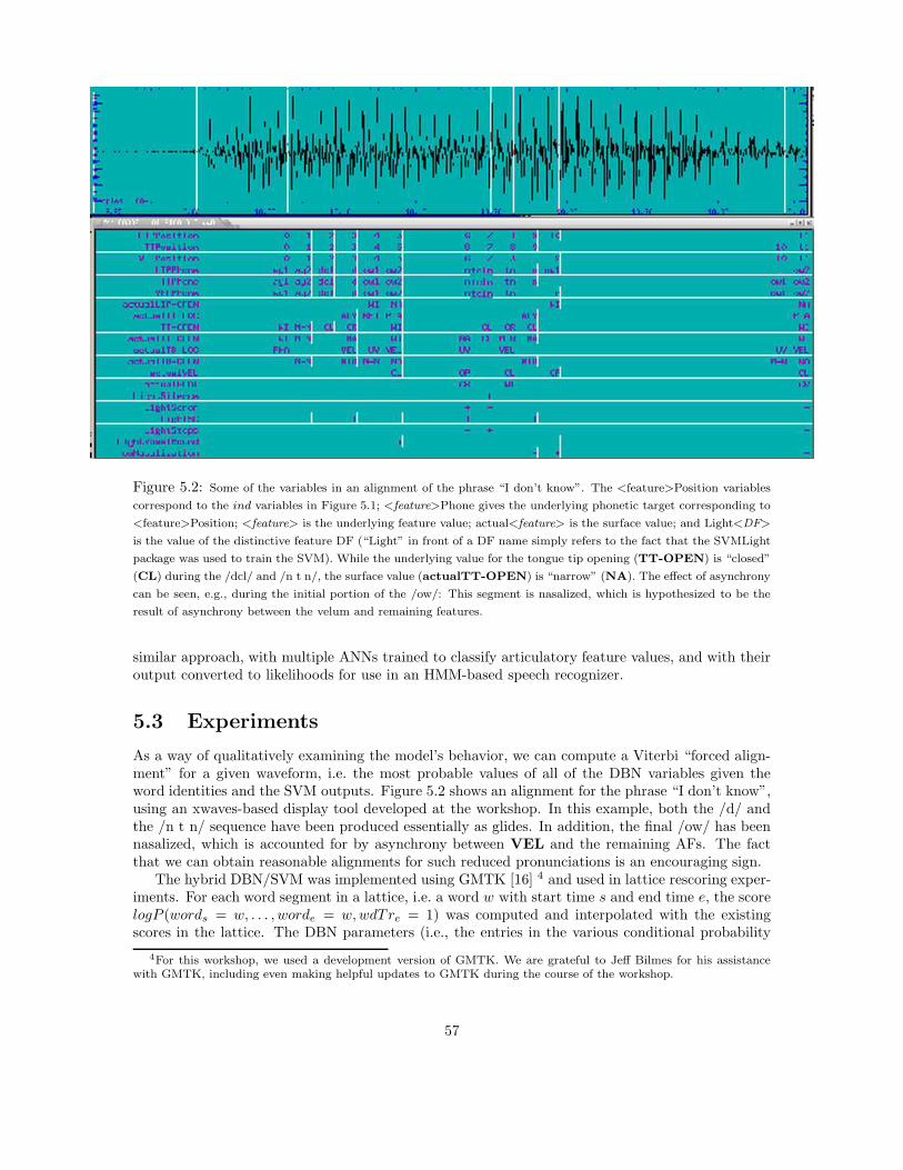
Figure 5.2: Some of the variables in an alignment of the phrase “I don’t know”. The <feature>Position variables

correspond to the ind variables in Figure 5.1; <feature>Phone gives the underlying phonetic target corresponding to

<feature>Position; <feature> is the underlying feature value; actual<feature> is the surface value; and Light<DF>

is the value of the distinctive feature DF (“Light” in front of a DF name simply refers to the fact that the SVMLight

package was used to train the SVM). While the underlying value for the tongue tip opening (TT-OPEN) is “closed”

(CL) during the /dcl/ and /n t n/, the surface value (actualTT-OPEN) is “narrow” (NA). The effect of asynchrony

can be seen, e.g., during the initial portion of the /ow/: This segment is nasalized, which is hypothesized to be the

result of asynchrony between the velum and remaining features.

similar approach, with multiple ANNs trained to classify articulatory feature values, and with theiroutput converted to likelihoods for use in an HMM-based speech recognizer.

5.3 Experiments

As a way of qualitatively examining the model’s behavior, we can compute a Viterbi “forced align-ment” for a given waveform, i.e. the most probable values of all of the DBN variables given theword identities and the SVM outputs. Figure 5.2 shows an alignment for the phrase “I don’t know”,using an xwaves-based display tool developed at the workshop. In this example, both the /d/ andthe /n t n/ sequence have been produced essentially as glides. In addition, the final /ow/ has beennasalized, which is accounted for by asynchrony between VEL and the remaining AFs. The factthat we can obtain reasonable alignments for such reduced pronunciations is an encouraging sign.

The hybrid DBN/SVM was implemented using GMTK [16] 4 and used in lattice rescoring exper-iments. For each word segment in a lattice, i.e. a word w with start time s and end time e, the scorelogP (words = w, . . . , worde = w, wdTre = 1) was computed and interpolated with the existingscores in the lattice. The DBN parameters (i.e., the entries in the various conditional probability

4For this workshop, we used a development version of GMTK. We are grateful to Jeff Bilmes for his assistancewith GMTK, including even making helpful updates to GMTK during the course of the workshop.

57

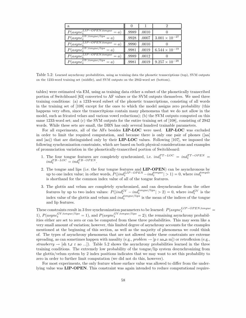
a 0 1 2

P (asyncLIP−OPEN ;tonguet = a) .9989 .0010 0

P (asyncGV ;tongue/lipst = a) .9928 .0007 3.001× 10−27

P (asyncLIP−OPEN ;tonguet = a) .9990 .0010 0

P (asyncGV ;tongue/lipst = a) .9981 .0019 6.544× 10−19

P (asyncLIP−OPEN ;tonguet = a) .9989 .0012 0

P (asyncGV ;tongue/lipst = a) .9981 .0019 9.257× 10−20

Table 5.2: Learned asynchrony probabilities, using as training data the phonetic transcriptions (top), SVM outputs

on the 1233-word training set (middle), and SVM outputs on the 2942-word set (bottom).

tables) were estimated via EM, using as training data either a subset of the phonetically transcribedportion of Switchboard [63] converted to AF values or the SVM outputs themselves. We used threetraining conditions: (a) a 1233-word subset of the phonetic transcriptions, consisting of all wordsin the training set of [108] except for the ones to which the model assigns zero probability (thishappens very often, since the transcritpions contain many phenomena that we do not allow in themodel, such as fricated velars and various vowel reductions); (b) the SVM outputs computed on thissame 1233-word set; and (c) the SVM outputs for the entire training set of [108], consisting of 2942words. While these sets are small, the DBN has only several hundred trainable parameters.

For all experiments, all of the AFs besides LIP-LOC were used. LIP-LOC was excludedin order to limit the required computation, and because there is only one pair of phones ([aa]and [ao]) that are distinguished only by their LIP-LOC values. Following [107], we imposed thefollowing synchronization constraints, which are based on both physical considerations and examplesof pronunciation variation in the phonetically-transcribed portion of Switchboard:

1. The four tongue features are completely synchronized, i.e. indTT−LOCt = indTT−OPEN

t =indTB−LOC

t = indTB−OPENt .

2. The tongue and lips (i.e. the four tongue features and LIP-OPEN) can be asynchronous byup to one index value; in other words, P (|indLIP−OPEN

t −indtonguet | > 1) = 0, where indtongue

t

is shorthand for the common index value of all of the tongue features.

3. The glottis and velum are completely synchronized, and can desynchronize from the other

features by up to two index values: P (|indGVt − ind

tongue/lipst | > 2) = 0, where indGV

t is the

index value of the glottis and velum and indtongue/lipst is the mean of the indices of the tongue

and lip features.

These constraints result in 3 free synchronization parameters to be learned: P (asyncLIP−OPEN ;tonguet =

1), P (asyncGV ;tongue/lipst = 1), and P (async

GV ;tongue/lipst = 2); the remaining asynchrony probabil-

ities either are set to zero or can be computed from these three probabilities. This may seem like avery small amount of variation; however, this limited degree of asynchrony accounts for the examplesmentioned at the beginning of this section, as well as the majority of phenomena we could thinkof. The types of asynchrony phenomena that are not allowed under these constraints are extremespreading, as can sometimes happen with nasality (e.g., problem → [p r aa n m]) or retroflexion (e.g.,strawberry → [sh t r r ao ...]). Table 5.2 shows the asynchrony probabilities learned in the threetraining conditions. The extremely low probability of the tongue/lip system desynchronizing fromthe glottis/velum system by 2 index positions indicates that we may want to set this probability tozero in order to further limit computation (we did not do this, however).

For most experiments, the only feature whose surface value was allowed to differ from the under-lying value was LIP-OPEN. This constraint was again intended to reduce computational require-

58

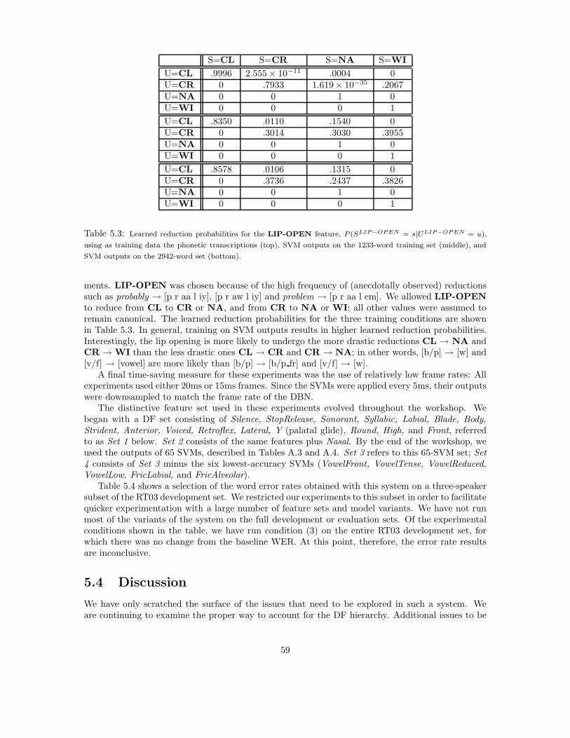
S=CL S=CR S=NA S=WI

U=CL .9996 2.555× 10−11 .0004 0U=CR 0 .7933 1.619× 10−35 .2067U=NA 0 0 1 0U=WI 0 0 0 1

U=CL .8350 .0110 .1540 0U=CR 0 .3014 .3030 .3955U=NA 0 0 1 0U=WI 0 0 0 1

U=CL .8578 .0106 .1315 0U=CR 0 .3736 .2437 .3826U=NA 0 0 1 0U=WI 0 0 0 1

Table 5.3: Learned reduction probabilities for the LIP-OPEN feature, P (SLIP−OPEN = s|ULIP−OPEN = u),

using as training data the phonetic transcriptions (top), SVM outputs on the 1233-word training set (middle), and

SVM outputs on the 2942-word set (bottom).

ments. LIP-OPEN was chosen because of the high frequency of (anecdotally observed) reductionssuch as probably → [p r aa l iy], [p r aw l iy] and problem → [p r aa l em]. We allowed LIP-OPEN

to reduce from CL to CR or NA, and from CR to NA or WI; all other values were assumed toremain canonical. The learned reduction probabilities for the three training conditions are shownin Table 5.3. In general, training on SVM outputs results in higher learned reduction probabilities.Interestingly, the lip opening is more likely to undergo the more drastic reductions CL → NA andCR → WI than the less drastic ones CL → CR and CR → NA; in other words, [b/p] → [w] and[v/f] → [vowel] are more likely than [b/p] → [b/p fr] and [v/f] → [w].

A final time-saving measure for these experiments was the use of relatively low frame rates: Allexperiments used either 20ms or 15ms frames. Since the SVMs were applied every 5ms, their outputswere downsampled to match the frame rate of the DBN.

The distinctive feature set used in these experiments evolved throughout the workshop. Webegan with a DF set consisting of Silence, StopRelease, Sonorant, Syllabic, Labial, Blade, Body,Strident, Anterior, Voiced, Retroflex, Lateral, Y (palatal glide), Round, High, and Front, referredto as Set 1 below. Set 2 consists of the same features plus Nasal. By the end of the workshop, weused the outputs of 65 SVMs, described in Tables A.3 and A.4. Set 3 refers to this 65-SVM set; Set4 consists of Set 3 minus the six lowest-accuracy SVMs (VowelFront, VowelTense, VowelReduced,VowelLow, FricLabial, and FricAlveolar).

Table 5.4 shows a selection of the word error rates obtained with this system on a three-speakersubset of the RT03 development set. We restricted our experiments to this subset in order to facilitatequicker experimentation with a large number of feature sets and model variants. We have not runmost of the variants of the system on the full development or evaluation sets. Of the experimentalconditions shown in the table, we have run condition (3) on the entire RT03 development set, forwhich there was no change from the baseline WER. At this point, therefore, the error rate resultsare inconclusive.

5.4 Discussion

We have only scratched the surface of the issues that need to be explored in such a system. Weare continuing to examine the proper way to account for the DF hierarchy. Additional issues to be

59

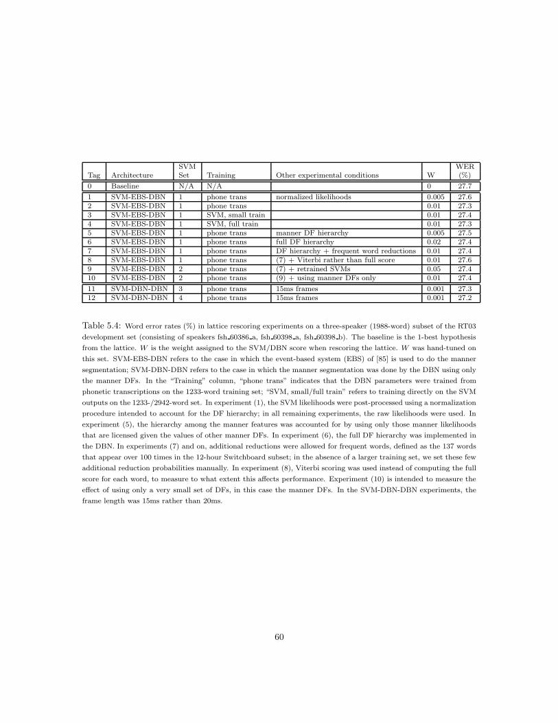
SVM WERTag Architecture Set Training Other experimental conditions W (%)

0 Baseline N/A N/A 0 27.7

1 SVM-EBS-DBN 1 phone trans normalized likelihoods 0.005 27.62 SVM-EBS-DBN 1 phone trans 0.01 27.33 SVM-EBS-DBN 1 SVM, small train 0.01 27.44 SVM-EBS-DBN 1 SVM, full train 0.01 27.35 SVM-EBS-DBN 1 phone trans manner DF hierarchy 0.005 27.56 SVM-EBS-DBN 1 phone trans full DF hierarchy 0.02 27.47 SVM-EBS-DBN 1 phone trans DF hierarchy + frequent word reductions 0.01 27.48 SVM-EBS-DBN 1 phone trans (7) + Viterbi rather than full score 0.01 27.69 SVM-EBS-DBN 2 phone trans (7) + retrained SVMs 0.05 27.410 SVM-EBS-DBN 2 phone trans (9) + using manner DFs only 0.01 27.4

11 SVM-DBN-DBN 3 phone trans 15ms frames 0.001 27.312 SVM-DBN-DBN 4 phone trans 15ms frames 0.001 27.2

Table 5.4: Word error rates (%) in lattice rescoring experiments on a three-speaker (1988-word) subset of the RT03

development set (consisting of speakers fsh 60386 a, fsh 60398 a, fsh 60398 b). The baseline is the 1-best hypothesis

from the lattice. W is the weight assigned to the SVM/DBN score when rescoring the lattice. W was hand-tuned on

this set. SVM-EBS-DBN refers to the case in which the event-based system (EBS) of [85] is used to do the manner

segmentation; SVM-DBN-DBN refers to the case in which the manner segmentation was done by the DBN using only

the manner DFs. In the “Training” column, “phone trans” indicates that the DBN parameters were trained from

phonetic transcriptions on the 1233-word training set; “SVM, small/full train” refers to training directly on the SVM

outputs on the 1233-/2942-word set. In experiment (1), the SVM likelihoods were post-processed using a normalization

procedure intended to account for the DF hierarchy; in all remaining experiments, the raw likelihoods were used. In

experiment (5), the hierarchy among the manner features was accounted for by using only those manner likelihoods

that are licensed given the values of other manner DFs. In experiment (6), the full DF hierarchy was implemented in

the DBN. In experiments (7) and on, additional reductions were allowed for frequent words, defined as the 137 words

that appear over 100 times in the 12-hour Switchboard subset; in the absence of a larger training set, we set these few

additional reduction probabilities manually. In experiment (8), Viterbi scoring was used instead of computing the full

score for each word, to measure to what extent this affects performance. Experiment (10) is intended to measure the

effect of using only a very small set of DFs, in this case the manner DFs. In the SVM-DBN-DBN experiments, the

frame length was 15ms rather than 20ms.

60

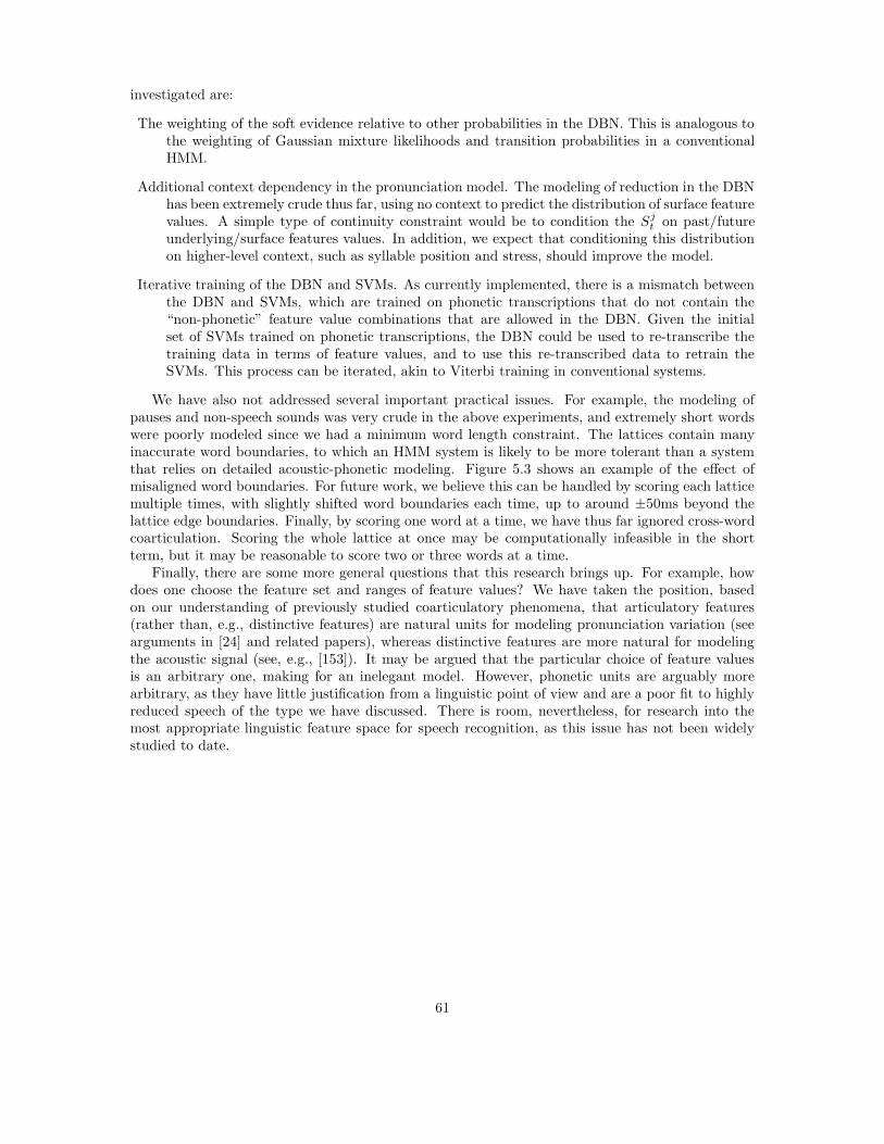
investigated are:

The weighting of the soft evidence relative to other probabilities in the DBN. This is analogous tothe weighting of Gaussian mixture likelihoods and transition probabilities in a conventionalHMM.

Additional context dependency in the pronunciation model. The modeling of reduction in the DBNhas been extremely crude thus far, using no context to predict the distribution of surface featurevalues. A simple type of continuity constraint would be to condition the Sj

t on past/futureunderlying/surface features values. In addition, we expect that conditioning this distributionon higher-level context, such as syllable position and stress, should improve the model.

Iterative training of the DBN and SVMs. As currently implemented, there is a mismatch betweenthe DBN and SVMs, which are trained on phonetic transcriptions that do not contain the“non-phonetic” feature value combinations that are allowed in the DBN. Given the initialset of SVMs trained on phonetic transcriptions, the DBN could be used to re-transcribe thetraining data in terms of feature values, and to use this re-transcribed data to retrain theSVMs. This process can be iterated, akin to Viterbi training in conventional systems.

We have also not addressed several important practical issues. For example, the modeling ofpauses and non-speech sounds was very crude in the above experiments, and extremely short wordswere poorly modeled since we had a minimum word length constraint. The lattices contain manyinaccurate word boundaries, to which an HMM system is likely to be more tolerant than a systemthat relies on detailed acoustic-phonetic modeling. Figure 5.3 shows an example of the effect ofmisaligned word boundaries. For future work, we believe this can be handled by scoring each latticemultiple times, with slightly shifted word boundaries each time, up to around ±50ms beyond thelattice edge boundaries. Finally, by scoring one word at a time, we have thus far ignored cross-wordcoarticulation. Scoring the whole lattice at once may be computationally infeasible in the shortterm, but it may be reasonable to score two or three words at a time.

Finally, there are some more general questions that this research brings up. For example, howdoes one choose the feature set and ranges of feature values? We have taken the position, basedon our understanding of previously studied coarticulatory phenomena, that articulatory features(rather than, e.g., distinctive features) are natural units for modeling pronunciation variation (seearguments in [24] and related papers), whereas distinctive features are more natural for modelingthe acoustic signal (see, e.g., [153]). It may be argued that the particular choice of feature valuesis an arbitrary one, making for an inelegant model. However, phonetic units are arguably morearbitrary, as they have little justification from a linguistic point of view and are a poor fit to highlyreduced speech of the type we have discussed. There is room, nevertheless, for research into themost appropriate linguistic feature space for speech recognition, as this issue has not been widelystudied to date.

61

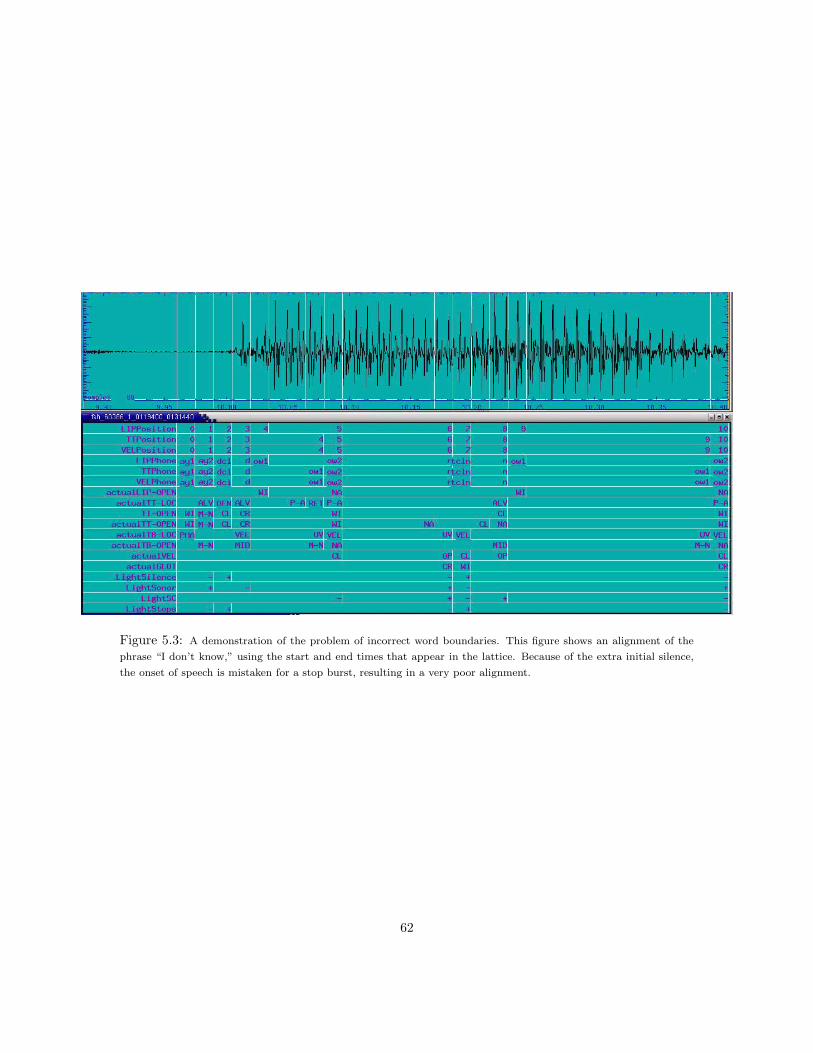
Figure 5.3: A demonstration of the problem of incorrect word boundaries. This figure shows an alignment of the

phrase “I don’t know,” using the start and end times that appear in the lattice. Because of the extra initial silence,

the onset of speech is mistaken for a stop burst, resulting in a very poor alignment.

62

Chapter 6

Discriminative Rescoring Using

Landmarks

As an alternative to a generative model, which seeks to model the articulatory process by whichlandmarks are produced, we also used landmark information in a discriminative way, i.e. in orderto distinguish between confusable word hypotheses output by a baseline recognizer. Under thisapproach, not all landmark features are used at all times; only those landmarks are used that arenecessary to identify correct word hypotheses in the presence of competing incorrect hypotheses.After the relevant landmarks have been identified, scores are requested for them from the lower-levellandmark detectors. These are then used for rescoring the output from the baseline recognizer.Thus, the general procedure is the following:

1. use a baseline recognizer to produce word lattices;

2. convert lattices into confusion networks;

3. train a discriminative model based on word pronunciations to identify the most relevant land-marks;

4. obtain scores for those landmarks using lower-level landmark detectors;

5. rescore the baseline hypotheses and produce new 1-best word sequences.

The data set that was used for the experiments described below was the RT03 evaluation set.This set consisted of 35497 words and 2930 segments (utterances), produced by 36 speakers. As abaseline recognizer, the SRI DECIPHERTMsystem was used. A basic description of the system canbe found in e.g. [166]. Its output consisted of HTK-style word lattices containing the start and endtimes as well as the pronunciations (phone strings) of each word hypothesis, as well as the acousticand language model scores. The baseline word error rate, obtained from N-best lists generated fromthe lattices, was 24.4%; the oracle error rate was 16.2%. Note that the baseline word error rate isbased on recognition with a a pronunciation model (different pronunciation variants specified in thelexicon), duration modeling, a 4-gram language model, and speaker-adapted acoustic models. Thebaseline system thus is a state-of-the-art system which already succeeds at modeling much of thepronunciation variation inherent in the data.

6.1 Conversion to Confusion Networks

The lattices produced by the baseline recognizer were subsequently converted into confusion net-works, i.e. word networks representing confusable word hypotheses on parallel arcs between two

63

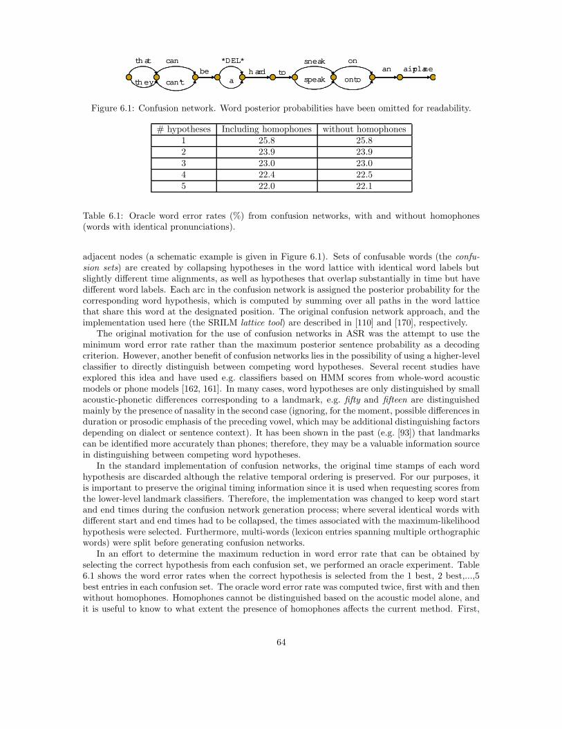
airplaneanon

onto

sneak

speaktohard

*DEL*be

that can

can’t athey

airplaneanon

onto

sneak

speaktohard

*DEL*be

that can

can’t athey

Figure 6.1: Confusion network. Word posterior probabilities have been omitted for readability.

# hypotheses Including homophones without homophones1 25.8 25.82 23.9 23.93 23.0 23.04 22.4 22.55 22.0 22.1

Table 6.1: Oracle word error rates (%) from confusion networks, with and without homophones(words with identical pronunciations).

adjacent nodes (a schematic example is given in Figure 6.1). Sets of confusable words (the confu-sion sets) are created by collapsing hypotheses in the word lattice with identical word labels butslightly different time alignments, as well as hypotheses that overlap substantially in time but havedifferent word labels. Each arc in the confusion network is assigned the posterior probability for thecorresponding word hypothesis, which is computed by summing over all paths in the word latticethat share this word at the designated position. The original confusion network approach, and theimplementation used here (the SRILM lattice tool) are described in [110] and [170], respectively.

The original motivation for the use of confusion networks in ASR was the attempt to use theminimum word error rate rather than the maximum posterior sentence probability as a decodingcriterion. However, another benefit of confusion networks lies in the possibility of using a higher-levelclassifier to directly distinguish between competing word hypotheses. Several recent studies haveexplored this idea and have used e.g. classifiers based on HMM scores from whole-word acousticmodels or phone models [162, 161]. In many cases, word hypotheses are only distinguished by smallacoustic-phonetic differences corresponding to a landmark, e.g. fifty and fifteen are distinguishedmainly by the presence of nasality in the second case (ignoring, for the moment, possible differences induration or prosodic emphasis of the preceding vowel, which may be additional distinguishing factorsdepending on dialect or sentence context). It has been shown in the past (e.g. [93]) that landmarkscan be identified more accurately than phones; therefore, they may be a valuable information sourcein distinguishing between competing word hypotheses.

In the standard implementation of confusion networks, the original time stamps of each wordhypothesis are discarded although the relative temporal ordering is preserved. For our purposes, itis important to preserve the original timing information since it is used when requesting scores fromthe lower-level landmark classifiers. Therefore, the implementation was changed to keep word startand end times during the confusion network generation process; where several identical words withdifferent start and end times had to be collapsed, the times associated with the maximum-likelihoodhypothesis were selected. Furthermore, multi-words (lexicon entries spanning multiple orthographicwords) were split before generating confusion networks.

In an effort to determine the maximum reduction in word error rate that can be obtained byselecting the correct hypothesis from each confusion set, we performed an oracle experiment. Table6.1 shows the word error rates when the correct hypothesis is selected from the 1 best, 2 best,...,5best entries in each confusion set. The oracle word error rate was computed twice, first with and thenwithout homophones. Homophones cannot be distinguished based on the acoustic model alone, andit is useful to know to what extent the presence of homophones affects the current method. First,

64

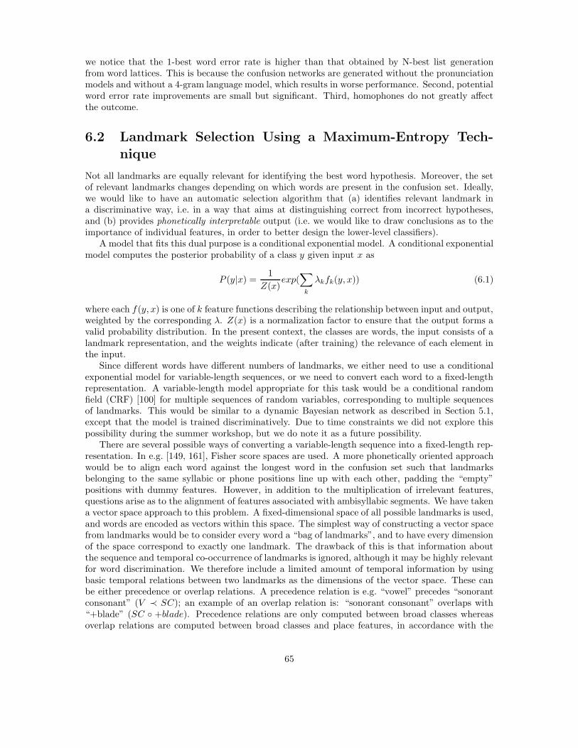
we notice that the 1-best word error rate is higher than that obtained by N-best list generationfrom word lattices. This is because the confusion networks are generated without the pronunciationmodels and without a 4-gram language model, which results in worse performance. Second, potentialword error rate improvements are small but significant. Third, homophones do not greatly affectthe outcome.

6.2 Landmark Selection Using a Maximum-Entropy Tech-

nique

Not all landmarks are equally relevant for identifying the best word hypothesis. Moreover, the setof relevant landmarks changes depending on which words are present in the confusion set. Ideally,we would like to have an automatic selection algorithm that (a) identifies relevant landmark ina discriminative way, i.e. in a way that aims at distinguishing correct from incorrect hypotheses,and (b) provides phonetically interpretable output (i.e. we would like to draw conclusions as to theimportance of individual features, in order to better design the lower-level classifiers).

A model that fits this dual purpose is a conditional exponential model. A conditional exponentialmodel computes the posterior probability of a class y given input x as

P (y|x) =1

Z(x)exp(

∑

k

λkfk(y, x)) (6.1)

where each f(y, x) is one of k feature functions describing the relationship between input and output,weighted by the corresponding λ. Z(x) is a normalization factor to ensure that the output forms avalid probability distribution. In the present context, the classes are words, the input consists of alandmark representation, and the weights indicate (after training) the relevance of each element inthe input.

Since different words have different numbers of landmarks, we either need to use a conditionalexponential model for variable-length sequences, or we need to convert each word to a fixed-lengthrepresentation. A variable-length model appropriate for this task would be a conditional randomfield (CRF) [100] for multiple sequences of random variables, corresponding to multiple sequencesof landmarks. This would be similar to a dynamic Bayesian network as described in Section 5.1,except that the model is trained discriminatively. Due to time constraints we did not explore thispossibility during the summer workshop, but we do note it as a future possibility.

There are several possible ways of converting a variable-length sequence into a fixed-length rep-resentation. In e.g. [149, 161], Fisher score spaces are used. A more phonetically oriented approachwould be to align each word against the longest word in the confusion set such that landmarksbelonging to the same syllabic or phone positions line up with each other, padding the “empty”positions with dummy features. However, in addition to the multiplication of irrelevant features,questions arise as to the alignment of features associated with ambisyllabic segments. We have takena vector space approach to this problem. A fixed-dimensional space of all possible landmarks is used,and words are encoded as vectors within this space. The simplest way of constructing a vector spacefrom landmarks would be to consider every word a “bag of landmarks”, and to have every dimensionof the space correspond to exactly one landmark. The drawback of this is that information aboutthe sequence and temporal co-occurrence of landmarks is ignored, although it may be highly relevantfor word discrimination. We therefore include a limited amount of temporal information by usingbasic temporal relations between two landmarks as the dimensions of the vector space. These canbe either precedence or overlap relations. A precedence relation is e.g. “vowel” precedes “sonorantconsonant” (V ≺ SC); an example of an overlap relation is: “sonorant consonant” overlaps with“+blade” (SC ◦ +blade). Precedence relations are only computed between broad classes whereasoverlap relations are computed between broad classes and place features, in accordance with the

65

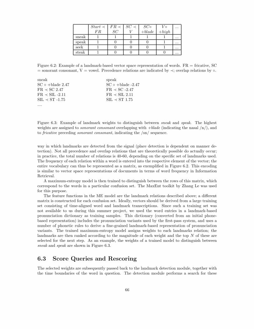
Start ≺ FR ≺ SC ≺ SC◦ V ◦ ...FR SC V +blade +high

sneak 1 1 1 1 1 ...speak 1 0 0 0 1 ...seek 1 0 0 0 1 ...steak 1 0 0 0 0 ...

Figure 6.2: Example of a landmark-based vector space representation of words. FR = fricative, SC= sonorant consonant, V = vowel. Precedence relations are indicated by ≺; overlap relations by ◦.

sneak speakSC ◦ +blade 2.47 SC ◦ +blade -2.47FR ≺ SC 2.47 FR ≺ SC -2.47FR ≺ SIL -2.11 FR ≺ SIL 2.11SIL ≺ ST -1.75 SIL ≺ ST 1.75....

Figure 6.3: Example of landmark weights to distinguish between sneak and speak. The highestweights are assigned to sonorant consonant overlapping with +blade (indicating the nasal /n/), andto fricative preceding sonorant consonant, indicating the /sn/ sequence.

way in which landmarks are detected from the signal (place detection is dependent on manner de-tection). Not all precedence and overlap relations that are theoretically possible do actually occur;in practice, the total number of relations is 40-60, depending on the specific set of landmarks used.The frequency of each relation within a word is entered into the respective element of the vector; theentire vocabulary can thus be represented as a matrix, as exemplified in Figure 6.2. This encodingis similar to vector space representations of documents in terms of word frequency in InformationRetrieval.

A maximum-entropy model is then trained to distinguish between the rows of this matrix, whichcorrespond to the words in a particular confusion set. The MaxEnt toolkit by Zhang Le was usedfor this purpose.

The feature functions in the ME model are the landmark relations described above; a differentmatrix is constructed for each confusion set. Ideally, vectors should be derived from a large trainingset consisting of time-aligned word and landmark transcriptions. Since such a training set wasnot available to us during this summer project, we used the word entries in a landmark-basedpronunciation dictionary as training samples. This dictionary (converted from an initial phone-based representation) includes the pronunciation variants used by the first-pass system, and uses anumber of phonetic rules to derive a fine-grained landmark-based representation of pronunciationvariants. The trained maximum-entropy model assigns weights to each landmarks relation; thelandmarks are then ranked according to the magnitude of each weight and the top N of these areselected for the next step. As an example, the weights of a trained model to distinguish betweensneak and speak are shown in Figure 6.3.

6.3 Score Queries and Rescoring

The selected weights are subsequently passed back to the landmark detection module, together withthe time boundaries of the word in question. The detection module performs a search for these

66

landmarks within the specified time constraints and returns their log-likelihood (see Sec. 4.9).Rescoring was done by a weighted combination of the baseline posterior probabilities and the

normalized acoustic landmark scores (weights 0.8 and 0.2, respectively). This process was onlyapplied to those confusion sets that contained phonetically distinguishable hypotheses (i.e. not tosets containing only homophones, such as buy - by, two - to - too, etc.), and only to those thatdid not contain the DELETE symbol. The DELETE symbol stands for a word deletion, and it isunclear how a meaningful landmark score could be assigned to it.

A number of additional options for rescoring were investigated during the course of this project:

• different sets of landmark features were used, in accordance with changes in the landmarkdetection framework

• number of hypotheses: only the top two vs. the top three vs. all hypotheses in the confusionset were considered

• time intervals: the entire word time interval was used for obtaining the required landmarkscores vs. a narrower time interval that corresponded more closely to the approximate locationof landmarks. This might be useful for word-initial or word-final landmarks – in those cases,better scores might be obtained when the signal portion to be scanned by the landmark detectoris narrowed down.

• number of landmark scores to use: only the landmark with the largest weight vs. the top twolandmarks vs. all landmarks

• weighting schemes: one weight for all landmark scores vs. different weights for manner vs. placefeatures

• score combination method: weighted sum of scores vs. weighted product of scores vs. themaximum-entropy score combination method described in the following chapter

The best word sequence (according to the rescored scores) was selected from the confusion networksand was evaluated.

6.4 Results and Analysis

In all cases, rescoring showed no change in word error rate. The number of word errors decreasedslightly but not sufficiently to yield a noticeable change in error rate. The decision about the correcthypothesis changed in about 8% of all cases. Many word errors, especially confusions, were fixed,but new errors were created as well. Overall, the number of repaired errors outweighed the numberof new errors slightly, but not sufficiently to produce a change in word error rate.

The analysis of errors showed that the method works well when the correct discriminating land-marks are identified, and when these landmarks can be robustly detected from the speech signal.For instance, the maxent model will identify SC ◦ nasal as the relevant landmark relation in order tochoose between mean (correct) and me (false). If the score for this relation is relatively high, say 0.75,the correct word will be chosen. However, the choice of the discriminating landmarks sometimesleads to problems. For instance, SIL ◦ +blade (denoting a voiceless alveolar stop) was identifiedas the relevant landmark to distinguish between once (correct) and what (false). The lexicon entryfor once did not contain a voiceless stop, but a voiceless alveolar epenthetic stop frequently occursin pronunciations of this word when the soft palate is closed (ending the /n/) prior to the openingof the alveolar constriction (beginning the /s/). If the landmark pair SIL ◦ +blade receives a highscore from the landmark detector, the wrong hypothesis, what, will be preferred. A similar problemarises with pronunciation variants like can’t ([kat]) – based on its lexicon entry, can’t gives rise todistinguishing landmark pairs like SC ◦ +nasal; however, in the actual pronunciation, the sonorant

67

consonant has been lost and the nasality feature now overlaps with the adjacent vowel. As a result,the landmark pair will receive a low score from the landmark detector. A second type of erroroccurs when the correct distinguishing landmarks have been identified, but the landmark detectorsare quite simply errorful (though confident). Finally, many incorrect landmark scores are caused byword edge effects: distinguishing e.g. he and she in the context of the preceding word much (withoutintervening pause) is nearly impossible. Since landmarks can be hypothesized for very small timeintervals, correct word start and end times are essential.

6.5 Conclusions

The first of the three problems described above (lexical representations and pronunciation variants)can be overcome by learning the appropriate landmark representations for words from data ratherthan taking them from the lexicon. As mentioned above, this was not possible during this projectbecause of the lack of landmark detection output and word alignments for the entire training set.The second problem requires improvements to the landmark detectors. Unfortunately, it was notpossible to measure the accuracy of the landmark detectors on the data that was used for the large-vocabulary experiments because of the lack of manual reference annotations. Thus, there is notassessment of how well the landmark detectors performed on our actual test set. Another problemis that the model relies on a small number of landmarks which are detected in an entirely bottom-up manner. This may lead to a large number of errors. It would be desirable to include moretop-down constraints into the landmark detection process, or to include more temporal constraintsinto the maximum-entropy landmark selection process (e.g. relations between three rather thantwo landmarks). The third problem is more difficult to solve – the word boundaries may oftenbe incorrect due to the choice of one particular start and end time during the confusion networkgeneration process (see above). A possible alternative would be to keep a record of the start andend times of all word hypotheses that were collapsed into the confusion set in question, and to sumthe landmark scores over all time intervals, thus treating the time alignment as a random variable.

An additional benefit of the proposed method is that it can be used with classifiers other thanlandmark detectors, e.g. with high-accuracy triphone classifiers. The advantage is that the weightsof the trained maximum-entropy model are amenable to human inspection and allow the mostrelevant elements of the lexical representation to be identified. This can serve as a diagnostic toolfor improving the performance of a given recognition system on a given task: the statistics of thescore queries, averaged over the entire test set, will point to those phonetic distinctions that areutilized most frequently in order to identify the correct word hypotheses. Finally, rescoring witha small number of selected landmarks is extremely fast and requires little computation; it wouldtherefore be possible to use this method in a real-time system.

68

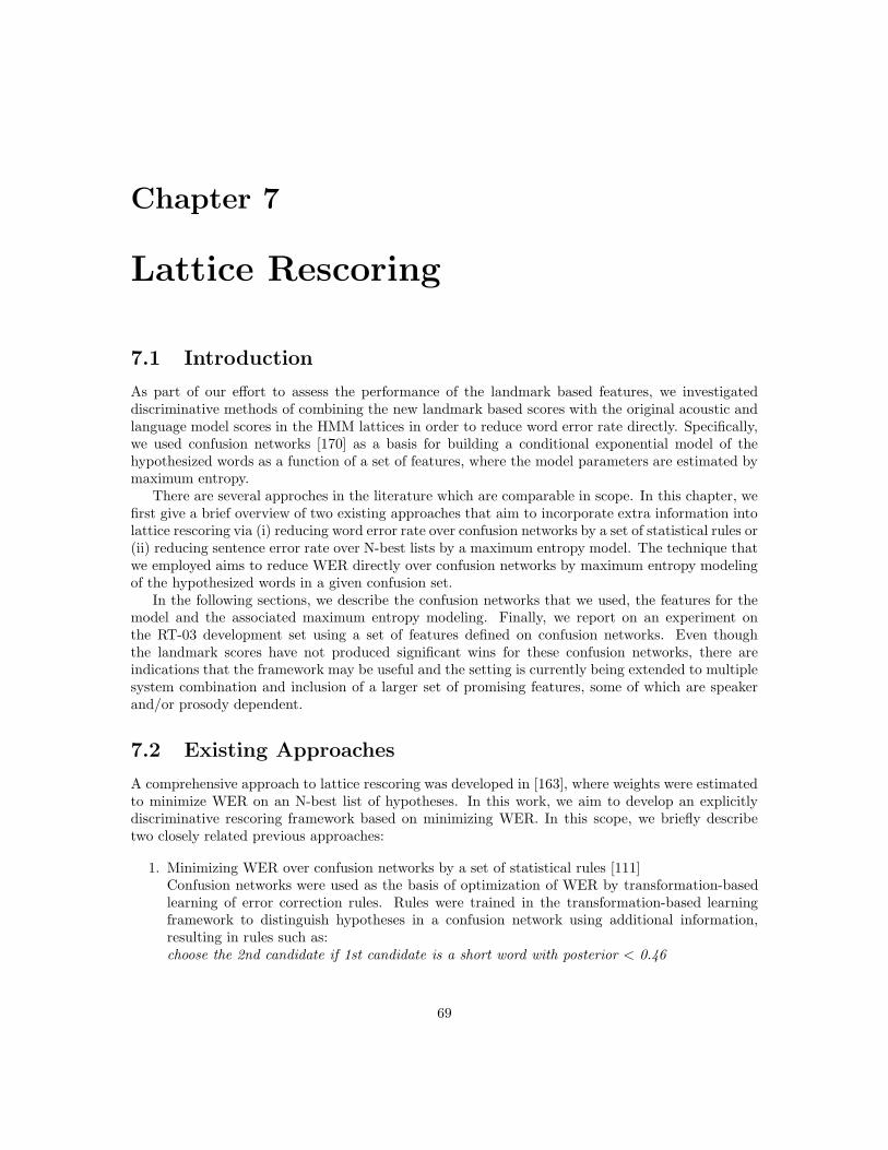
Chapter 7

Lattice Rescoring

7.1 Introduction

As part of our effort to assess the performance of the landmark based features, we investigateddiscriminative methods of combining the new landmark based scores with the original acoustic andlanguage model scores in the HMM lattices in order to reduce word error rate directly. Specifically,we used confusion networks [170] as a basis for building a conditional exponential model of thehypothesized words as a function of a set of features, where the model parameters are estimated bymaximum entropy.

There are several approches in the literature which are comparable in scope. In this chapter, wefirst give a brief overview of two existing approaches that aim to incorporate extra information intolattice rescoring via (i) reducing word error rate over confusion networks by a set of statistical rules or(ii) reducing sentence error rate over N-best lists by a maximum entropy model. The technique thatwe employed aims to reduce WER directly over confusion networks by maximum entropy modelingof the hypothesized words in a given confusion set.

In the following sections, we describe the confusion networks that we used, the features for themodel and the associated maximum entropy modeling. Finally, we report on an experiment onthe RT-03 development set using a set of features defined on confusion networks. Even thoughthe landmark scores have not produced significant wins for these confusion networks, there areindications that the framework may be useful and the setting is currently being extended to multiplesystem combination and inclusion of a larger set of promising features, some of which are speakerand/or prosody dependent.

7.2 Existing Approaches

A comprehensive approach to lattice rescoring was developed in [163], where weights were estimatedto minimize WER on an N-best list of hypotheses. In this work, we aim to develop an explicitlydiscriminative rescoring framework based on minimizing WER. In this scope, we briefly describetwo closely related previous approaches:

1. Minimizing WER over confusion networks by a set of statistical rules [111]Confusion networks were used as the basis of optimization of WER by transformation-basedlearning of error correction rules. Rules were trained in the transformation-based learningframework to distinguish hypotheses in a confusion network using additional information,resulting in rules such as:choose the 2nd candidate if 1st candidate is a short word with posterior < 0.46

69

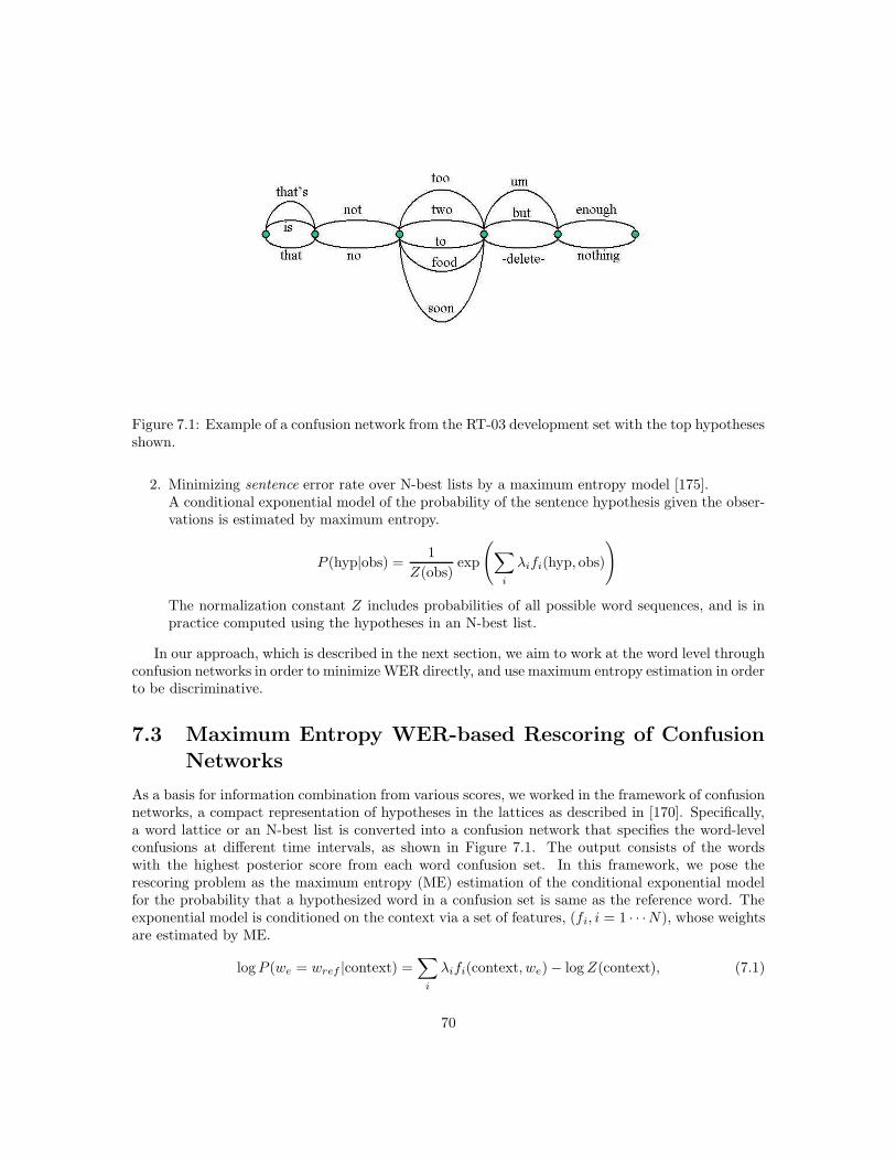
Figure 7.1: Example of a confusion network from the RT-03 development set with the top hypothesesshown.

2. Minimizing sentence error rate over N-best lists by a maximum entropy model [175].A conditional exponential model of the probability of the sentence hypothesis given the obser-vations is estimated by maximum entropy.

P (hyp|obs) =1

Z(obs)exp

(

∑

i

λifi(hyp, obs)

)

The normalization constant Z includes probabilities of all possible word sequences, and is inpractice computed using the hypotheses in an N-best list.

In our approach, which is described in the next section, we aim to work at the word level throughconfusion networks in order to minimize WER directly, and use maximum entropy estimation in orderto be discriminative.

7.3 Maximum Entropy WER-based Rescoring of Confusion

Networks

As a basis for information combination from various scores, we worked in the framework of confusionnetworks, a compact representation of hypotheses in the lattices as described in [170]. Specifically,a word lattice or an N-best list is converted into a confusion network that specifies the word-levelconfusions at different time intervals, as shown in Figure 7.1. The output consists of the wordswith the highest posterior score from each word confusion set. In this framework, we pose therescoring problem as the maximum entropy (ME) estimation of the conditional exponential modelfor the probability that a hypothesized word in a confusion set is same as the reference word. Theexponential model is conditioned on the context via a set of features, (fi, i = 1 · · ·N), whose weightsare estimated by ME.

log P (we = wref |context) =∑

i

λifi(context, we) − log Z(context), (7.1)

70

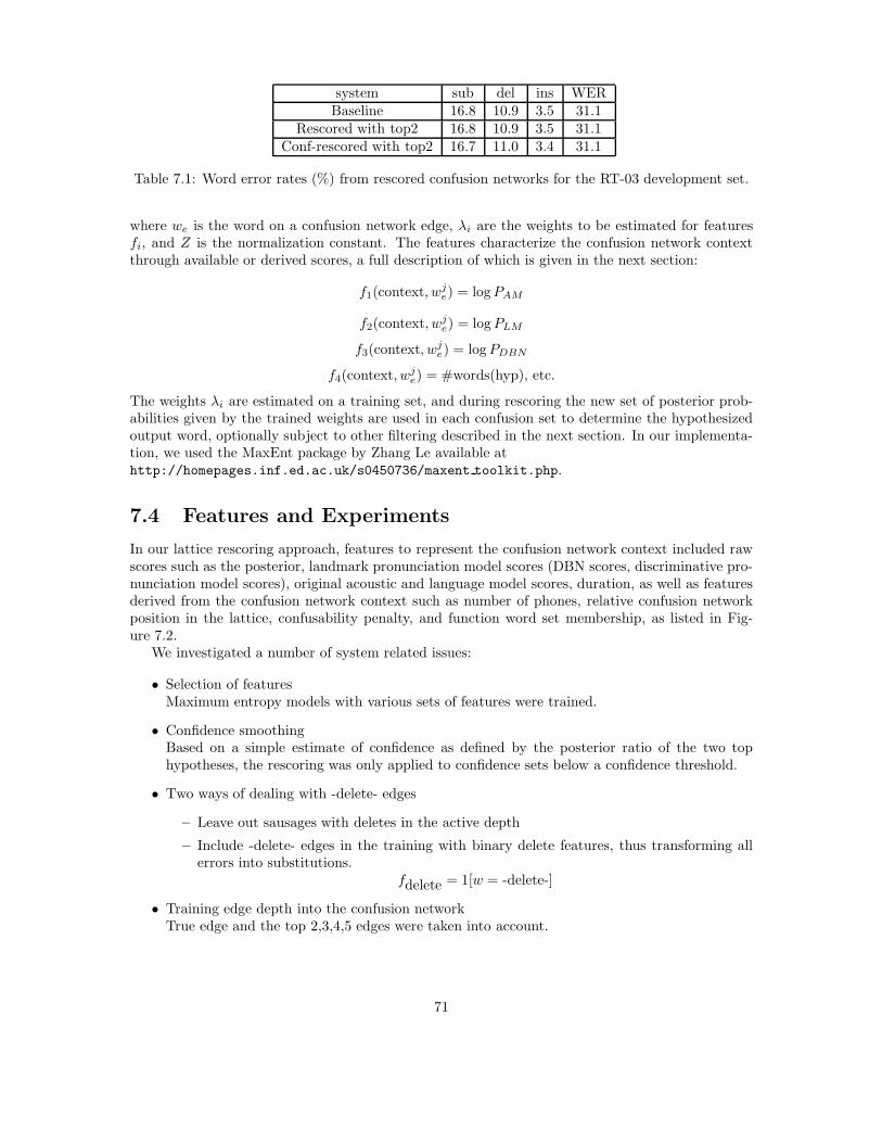
system sub del ins WERBaseline 16.8 10.9 3.5 31.1

Rescored with top2 16.8 10.9 3.5 31.1Conf-rescored with top2 16.7 11.0 3.4 31.1

Table 7.1: Word error rates (%) from rescored confusion networks for the RT-03 development set.

where we is the word on a confusion network edge, λi are the weights to be estimated for featuresfi, and Z is the normalization constant. The features characterize the confusion network contextthrough available or derived scores, a full description of which is given in the next section:

f1(context, wje) = log PAM

f2(context, wje) = log PLM

f3(context, wje) = log PDBN

f4(context, wje) = #words(hyp), etc.

The weights λi are estimated on a training set, and during rescoring the new set of posterior prob-abilities given by the trained weights are used in each confusion set to determine the hypothesizedoutput word, optionally subject to other filtering described in the next section. In our implementa-tion, we used the MaxEnt package by Zhang Le available athttp://homepages.inf.ed.ac.uk/s0450736/maxent toolkit.php.

7.4 Features and Experiments

In our lattice rescoring approach, features to represent the confusion network context included rawscores such as the posterior, landmark pronunciation model scores (DBN scores, discriminative pro-nunciation model scores), original acoustic and language model scores, duration, as well as featuresderived from the confusion network context such as number of phones, relative confusion networkposition in the lattice, confusability penalty, and function word set membership, as listed in Fig-ure 7.2.

We investigated a number of system related issues:

• Selection of featuresMaximum entropy models with various sets of features were trained.

• Confidence smoothingBased on a simple estimate of confidence as defined by the posterior ratio of the two tophypotheses, the rescoring was only applied to confidence sets below a confidence threshold.

• Two ways of dealing with -delete- edges

– Leave out sausages with deletes in the active depth

– Include -delete- edges in the training with binary delete features, thus transforming allerrors into substitutions.

fdelete = 1[w = -delete-]

• Training edge depth into the confusion networkTrue edge and the top 2,3,4,5 edges were taken into account.

71

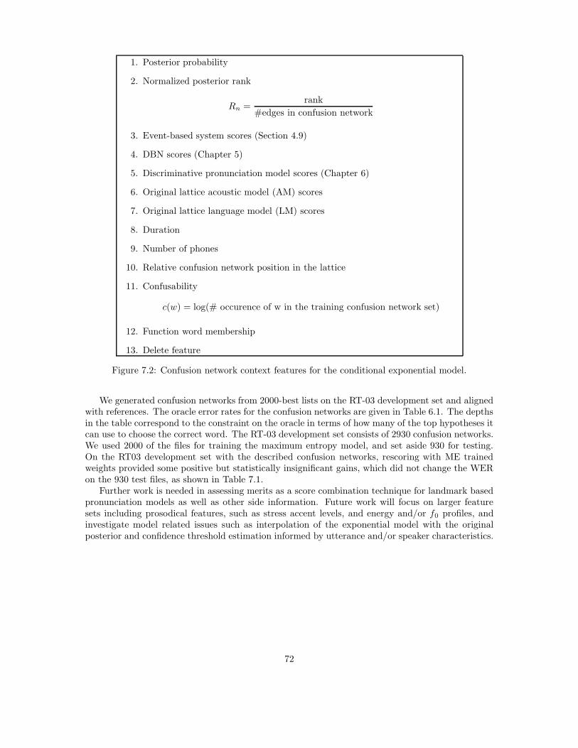
1. Posterior probability

2. Normalized posterior rank

Rn =rank

#edges in confusion network

3. Event-based system scores (Section 4.9)

4. DBN scores (Chapter 5)

5. Discriminative pronunciation model scores (Chapter 6)

6. Original lattice acoustic model (AM) scores

7. Original lattice language model (LM) scores

8. Duration

9. Number of phones

10. Relative confusion network position in the lattice

11. Confusability

c(w) = log(# occurence of w in the training confusion network set)

12. Function word membership

13. Delete feature

Figure 7.2: Confusion network context features for the conditional exponential model.

We generated confusion networks from 2000-best lists on the RT-03 development set and alignedwith references. The oracle error rates for the confusion networks are given in Table 6.1. The depthsin the table correspond to the constraint on the oracle in terms of how many of the top hypotheses itcan use to choose the correct word. The RT-03 development set consists of 2930 confusion networks.We used 2000 of the files for training the maximum entropy model, and set aside 930 for testing.On the RT03 development set with the described confusion networks, rescoring with ME trainedweights provided some positive but statistically insignificant gains, which did not change the WERon the 930 test files, as shown in Table 7.1.

Further work is needed in assessing merits as a score combination technique for landmark basedpronunciation models as well as other side information. Future work will focus on larger featuresets including prosodical features, such as stress accent levels, and energy and/or f0 profiles, andinvestigate model related issues such as interpolation of the exponential model with the originalposterior and confidence threshold estimation informed by utterance and/or speaker characteristics.

72

Chapter 8

Conclusions

Methods described in this report have resulted in WER reductions on an arbitrarily selected three-speaker subset of the target corpus, but no method applied to the entire corpus has resulted ina statistically significant WER reduction. Despite the current lack of a WER reduction, severalintermediate evaluation results support the argument in favor of further research along these lines.Rapid and continuous gains in phonetic classification accuracy were achieved, relative to the startof the workshop. The SVM was proven capable of learning classification boundaries in a very high-dimensional observation space, typically on the order of 500 to 2000 observation dimensions. TheDBN was shown capable of incorporating soft evidence computed by an SVM, and of using theavailable soft evidence to correctly transcribe consonant reductions.

Automatic classification of acoustic landmarks requires an algorithm capable of learning classi-fication boundaries in a high-dimensional observation space; SVMs satisfy the requirement. Prob-abilistic modeling of articulatory asynchrony requires an algorithm capable of learning the jointdistributions of many simultaneous hidden variables; DBNs satisfy the requirement. This report hasdemonstrated that it is possible to build an automatic speech recognizer that learns, from data, someof the information structures apparently used in human speech perception and speech production.

73

Appendix A

Appendices

A.1 Support Vector Machine Tutorial

Prior to start of the workshop, students participating in WS04 were given a brief tutorial in the useof support vector machines (SVMs) for acoustic phonetic classification and feature transformation.Key ideas from the tutorial are reproduced here. The review presented here is a brief subset ofmaterial also available from a number of other tutorials [25, 126].

An SVM is a regularized learning algorithm for binary classifiers [160]. A “regularized learner”is a learner whose optimality criterion balances training corpus error against classifier complexity;prior to the SVM, the most well-known regularized learning criterion was the Bayesian InformationCriterion (BIC) [145]. The term SVM is commonly used to describe both a regularized optimalitycriterion for binary classifiers, and the quadratic programming algorithm that solves it. Most SVMs(not all), like most neural networks, assume that the observation vector ~xm has some fixed dimension(~xm ∈ <K), and that the space of all possible classifiers can be represented by a single function

h(~xm, ~θ) ∈ {−1, 1}, where ~θ ∈ <D is a vector of real-valued trainable parameters. Most usefulbinary classifiers can be written as the binary quantization of a nonlinear discriminant functiong(~x, ~θ), thus

h(~x, ~θ) = sign(

g(~x, ~θ))

(A.1)

It is assumed, furthermore, that the vector of observations ~x is related to a binary truth-label y ∈{−1, 1} according to some unknown joint probability distribution p(~x, y). Under these assumptions,

the goal of machine learning is to choose a parameter vector ~θ that minimizes the expected error ofthe classifier (technically named the “risk”):

R(~θ) =∑

y∈{−1,1}

∫

u(−yg(~x, ~θ))dp(~x, y) (A.2)

where u(−yg) is the unit step function: a function that equals 1 whenever y and g have differentsigns, and is zero otherwise.

R(~θ) is the weighted average of the function u(−yg), with weights determined by the unknown

distribution p(~x, y). Because p(~x, y) is unknown, R(~θ) can not be computed; therefore it can not be

minimized. It is possible, however, to minimize upper bounds on R(~θ). A number of authors have

demonstrated upper bounds on R(~θ). In most cases, these upper bounds are derived by drawing Mindependent training samples of the form (~xm, ym) from the unknown distribution, measuring theaverage value of u(−yg) over the training samples, and then bounding the difference between theempirical training corpus error (known as the “empirical risk”) and the true risk [160, 74]. A typical

74

form of the upper bound is

R(~θ) ≤ Remp(~θ) + fδ

(

dV C

M

)

with probability ≥ 1 − δ (A.3)

where

Remp(~θ) =1

M

M∑

m=1

u(−ymg(~xm, ~θ)) (A.4)

and where the function fδ(dV C/M) usually grows slightly faster than linearly as a function ofdV C/M , and where the parameter dV C is called the V-C dimension of the classifier.

The V-C dimension measures the generalization flexibility of the classifier function h(). Eq. A.3therefore represents a “regularized” machine learning criterion, similar in many respects to theBayesian Information Criterion (BIC) [145]. The term Remp(~θ) measures the training corpus errorof the classifier; the term fδ(dV C/M) measures an upper bound (with probability 1 − δ) on thedifference between the training corpus and test corpus performance. In the version of Eq. A.3 usedby the BIC, dV C is estimated to be the number of trainable parameters of the classifier (dV C ≈ D).The estimate dV C ≈ D is useful for many classifier functions, but not all.

Vapnik and Chervonenkis studied the V-C dimension of the hyperplane classifier, whose discrim-inant function is given by

g(~x, ~w, b) = ~wT ~φ(~x) − b (A.5)

where ~φ(~x) ∈ <D−1 is a possibly nonlinear transformation of the input vector, and ~w ∈ <D−1 isa vector in the transformed space. Nonlinear hyperplane classifiers are typically constructed byperforming a basis expansion of the vector ~w, and then substituting a kernel computation in placeof the inner vector product, thus

~wT ~φ(~x) =

I∑

i=1

αi~φ(~µi)

T ~φ(~x) =

I∑

i=1

αiK(~µi, ~x) (A.6)

The parameters αi provide the basis expansion of ~w onto the vectors ~µi. In a kernel-based neuralnetwork, the vectors ~µi are often called “centers,” and their values can be adjusted using errorbackpropagation; in a non-parametric classifier such as an SVM, the centers are set equal to thetraining vectors, i.e., ~µi = ~xi. The kernel function K(~µ, ~x) can be almost any positive definitefunction, but two common functions are the “linear kernel” and the “radial basis function” or RBF:

LINEAR: K(~µ, ~x) = ~µT ~x (A.7)

RBF: K(~µ, ~x) = e−γ|~µ−~x|2 (A.8)

By using the kernel expansion (Eq. A.6), it is possible to define a hyperplane classifier in the space~φ(~x) without ever actually computing ~φ(~x). Therefore the dimension of ~φ(~x) can be much higherthan the dimension of ~x, or even infinite. The RBF kernel, for example, computes the dot product~φ(~µ)T ~φ(~x) in an infinite-dimensional implied space ~φ(~x).

Vapnik and Chervonenkis demonstrated two useful bounds on the V-C dimension of the hyper-plane classifier. First, there is an obvious bound, which is useful as long as the dimension of thetransformed vector ~φ(~x) is finite: dV C ≤ D − 1. Second, there is a less obvious bound, which is

useful if the magnitude of ~φ(~x) is bounded, even if its dimension is unbounded. Suppose that the

vectors ~φ(~x) are known to be bounded by |~φ(~x)| < R. Suppose also that we define a “forbiddenzone” near the hyperplane classifier. The “forbidden zone” has an adjustable width of r. Any vectorwithin the forbidden zone is counted as a partial error; thus, we define an error upper-bound function

75

u(−yg) ≥ u(−yg) that counts a partial error whenever the distance |g(~x, ~θ)|/|~w| < r:

u(−yg) =

{

0 yg > 01 yg < 0

, u(−yg)

= 0 yg|~w| ≥ r

> 0 yg|~w| < r

≥ 1 yg|~w| < 0

(A.9)

For the risk and empirical risk calculated using Eq. A.9, Vapnik and Chervonenkis showed that

dV C ≤

(

R

r

)2

(A.10)

We usually don’t know the true value of R. The standard SVM training criterion, therefore, has theform

RSV M (~θ) =C

M

M∑

m=1

u(−ymg(~xm, ~θ)) +

(

1

r

)2

(A.11)

where C is a “cost hyperparameter” or “regularization hyperparameter.” Algorithms for minimizingEq. A.11 are provided in a number of references [160, 25, 126], and efficient programs are publiclyavailable [84, 29].

In most SVM training experiments, C is chosen heuristically or by cross-validation experiments.Hastie et al. [73] have developed a theoretically well-grounded method for choosing the value of C,and their method was used in the workshop at WS04.

Fig. A.1 demonstrates the constraint placed on a hyperplane classifier by the requirement that allsamples counted as “correct” must be separated from the hyperplane by a distance of at least r. Inthe left-hand diagram, the hyperplane is allowed to pass within a distance of r = 0.1 from any of thetraining points. Under this constraint, it is possible to draw a hyperplane classifier that separatesthe training data with zero error. It would be foolish, however, to believe that the hyperplane shownwill also yield zero error on an independent test set: the tokens are very close to the separatrix, thusit is likely that the true class-dependent probability densities overlap. In the right-hand diagram,the hyperplane is not allowed to pass any closer than r = 0.33 to any of the training points. Underthis constraint, it is no longer possible to learn a classifier with zero training corpus error: the bestwe can achieve is a training corpus error of 5%. The training corpus error of 5%, however, is muchmore likely to accurately represent the true test corpus error of the classifier.

A.2 Articulatory Feature Set

Table A.1 defines the set of articulatory features used in the DBN model of pronunciation variability.

A.3 Phoneme-to-AF and AF-to-DF Mappings

Table A.2 defines the mapping from phonemes to articulatory features, as used by the DBN pronun-ciation model. Tables A.3 and A.4 describe the mapping from articulatory features to distinctivefeatures used by the hybrid SVM-DBN large vocabulary speech recognition system.

76

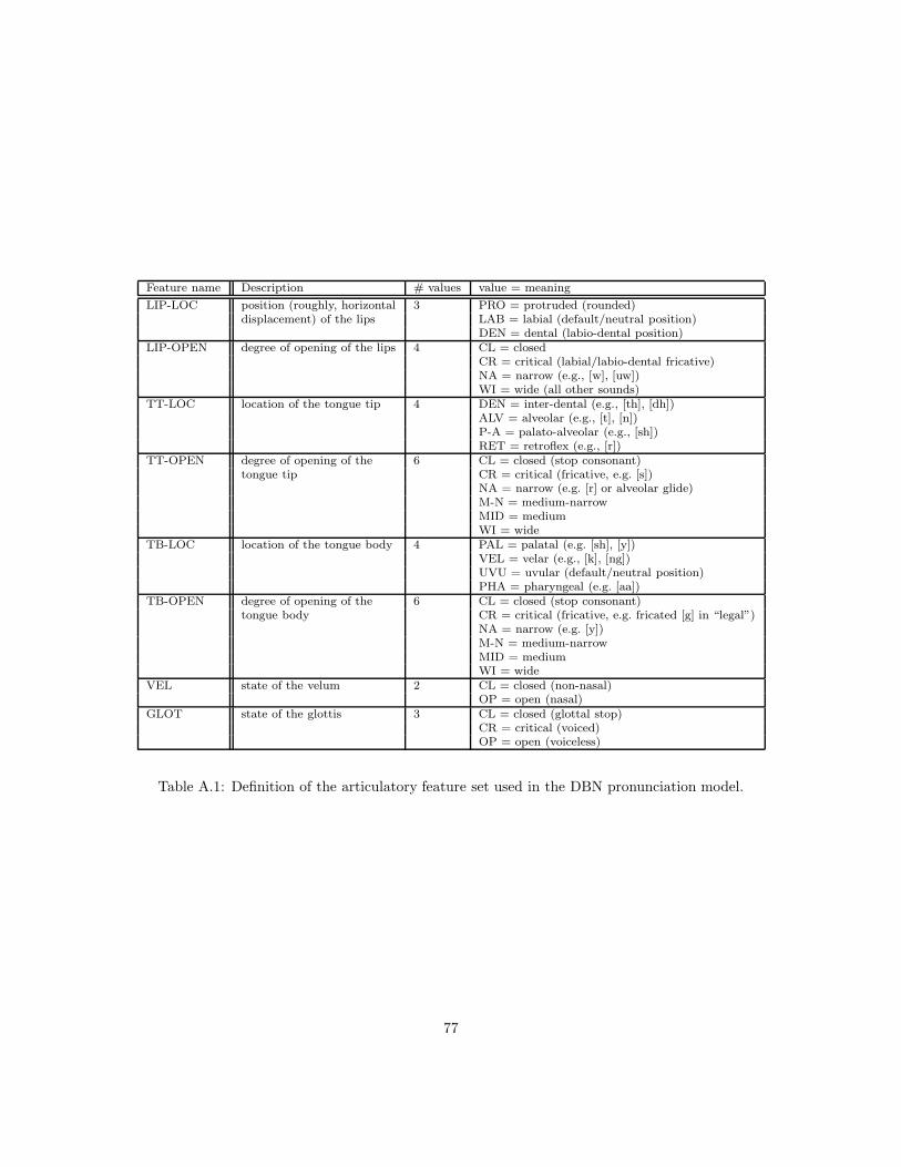
Feature name Description # values value = meaning

LIP-LOC position (roughly, horizontal 3 PRO = protruded (rounded)displacement) of the lips LAB = labial (default/neutral position)

DEN = dental (labio-dental position)LIP-OPEN degree of opening of the lips 4 CL = closed

CR = critical (labial/labio-dental fricative)NA = narrow (e.g., [w], [uw])WI = wide (all other sounds)

TT-LOC location of the tongue tip 4 DEN = inter-dental (e.g., [th], [dh])ALV = alveolar (e.g., [t], [n])P-A = palato-alveolar (e.g., [sh])RET = retroflex (e.g., [r])

TT-OPEN degree of opening of the 6 CL = closed (stop consonant)tongue tip CR = critical (fricative, e.g. [s])

NA = narrow (e.g. [r] or alveolar glide)M-N = medium-narrowMID = mediumWI = wide

TB-LOC location of the tongue body 4 PAL = palatal (e.g. [sh], [y])VEL = velar (e.g., [k], [ng])UVU = uvular (default/neutral position)PHA = pharyngeal (e.g. [aa])

TB-OPEN degree of opening of the 6 CL = closed (stop consonant)tongue body CR = critical (fricative, e.g. fricated [g] in “legal”)

NA = narrow (e.g. [y])M-N = medium-narrowMID = mediumWI = wide

VEL state of the velum 2 CL = closed (non-nasal)OP = open (nasal)

GLOT state of the glottis 3 CL = closed (glottal stop)CR = critical (voiced)OP = open (voiceless)

Table A.1: Definition of the articulatory feature set used in the DBN pronunciation model.

77

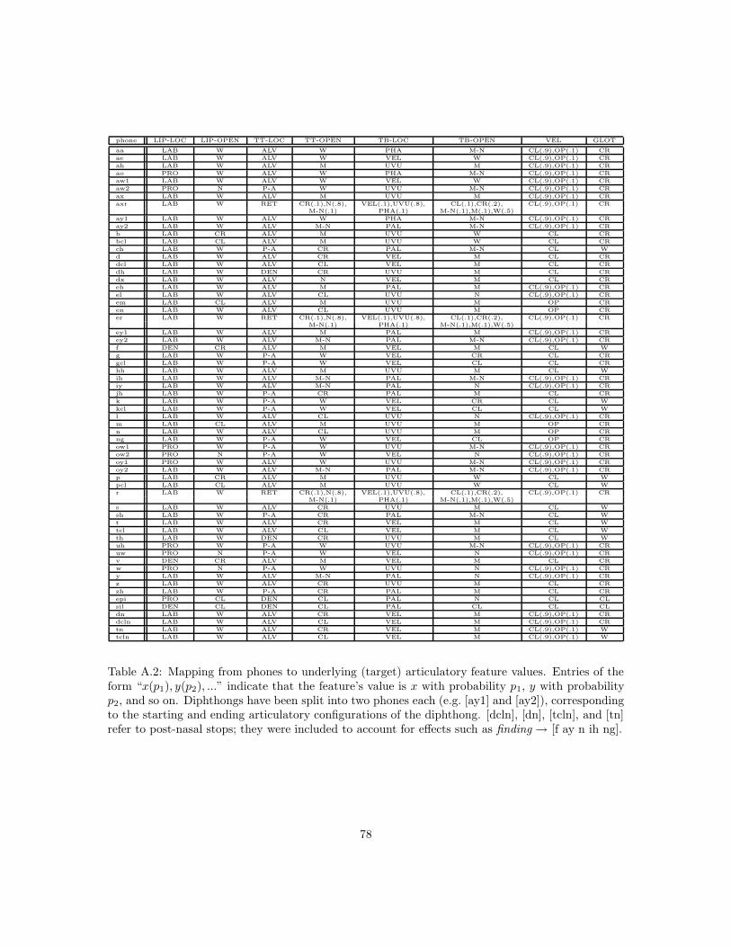
phone LIP-LOC LIP-OPEN TT-LOC TT-OPEN TB-LOC TB-OPEN VEL GLOT

aa LAB W ALV W PHA M-N CL(.9),OP(.1) CR

ae LAB W ALV W VEL W CL(.9),OP(.1) CR

ah LAB W ALV M UVU M CL(.9),OP(.1) CR

ao PRO W ALV W PHA M-N CL(.9),OP(.1) CR

aw1 LAB W ALV W VEL W CL(.9),OP(.1) CR

aw2 PRO N P-A W UVU M-N CL(.9),OP(.1) CR

ax LAB W ALV M UVU M CL(.9),OP(.1) CR

axr LAB W RET CR(.1),N(.8), VEL(.1),UVU(.8), CL(.1),CR(.2), CL(.9),OP(.1) CRM-N(.1) PHA(.1) M-N(.1),M(.1),W(.5)

ay1 LAB W ALV W PHA M-N CL(.9),OP(.1) CR

ay2 LAB W ALV M-N PAL M-N CL(.9),OP(.1) CR

b LAB CR ALV M UVU W CL CR

bcl LAB CL ALV M UVU W CL CR

ch LAB W P-A CR PAL M-N CL W

d LAB W ALV CR VEL M CL CR

dcl LAB W ALV CL VEL M CL CR

dh LAB W DEN CR UVU M CL CR

dx LAB W ALV N VEL M CL CR

eh LAB W ALV M PAL M CL(.9),OP(.1) CR

el LAB W ALV CL UVU N CL(.9),OP(.1) CR

em LAB CL ALV M UVU M OP CR

en LAB W ALV CL UVU M OP CR

er LAB W RET CR(.1),N(.8), VEL(.1),UVU(.8), CL(.1),CR(.2), CL(.9),OP(.1) CRM-N(.1) PHA(.1) M-N(.1),M(.1),W(.5)

ey1 LAB W ALV M PAL M CL(.9),OP(.1) CR

ey2 LAB W ALV M-N PAL M-N CL(.9),OP(.1) CR

f DEN CR ALV M VEL M CL W

g LAB W P-A W VEL CR CL CR

gcl LAB W P-A W VEL CL CL CR

hh LAB W ALV M UVU M CL W

ih LAB W ALV M-N PAL M-N CL(.9),OP(.1) CR

iy LAB W ALV M-N PAL N CL(.9),OP(.1) CR

jh LAB W P-A CR PAL M CL CR

k LAB W P-A W VEL CR CL W

kcl LAB W P-A W VEL CL CL W

l LAB W ALV CL UVU N CL(.9),OP(.1) CR

m LAB CL ALV M UVU M OP CR

n LAB W ALV CL UVU M OP CR

ng LAB W P-A W VEL CL OP CR

ow1 PRO W P-A W UVU M-N CL(.9),OP(.1) CR

ow2 PRO N P-A W VEL N CL(.9),OP(.1) CR

oy1 PRO W ALV W UVU M-N CL(.9),OP(.1) CR

oy2 LAB W ALV M-N PAL M-N CL(.9),OP(.1) CR

p LAB CR ALV M UVU W CL W

pcl LAB CL ALV M UVU W CL W

r LAB W RET CR(.1),N(.8), VEL(.1),UVU(.8), CL(.1),CR(.2), CL(.9),OP(.1) CRM-N(.1) PHA(.1) M-N(.1),M(.1),W(.5)

s LAB W ALV CR UVU M CL W

sh LAB W P-A CR PAL M-N CL W

t LAB W ALV CR VEL M CL W

tcl LAB W ALV CL VEL M CL W

th LAB W DEN CR UVU M CL W

uh PRO W P-A W UVU M-N CL(.9),OP(.1) CR

uw PRO N P-A W VEL N CL(.9),OP(.1) CR

v DEN CR ALV M VEL M CL CR

w PRO N P-A W UVU N CL(.9),OP(.1) CR

y LAB W ALV M-N PAL N CL(.9),OP(.1) CR

z LAB W ALV CR UVU M CL CR

zh LAB W P-A CR PAL M CL CR

epi PRO CL DEN CL PAL N CL CL

sil DEN CL DEN CL PAL CL CL CL

dn LAB W ALV CR VEL M CL(.9),OP(.1) CR

dcln LAB W ALV CL VEL M CL(.9),OP(.1) CR

tn LAB W ALV CR VEL M CL(.9),OP(.1) W

tcln LAB W ALV CL VEL M CL(.9),OP(.1) W

Table A.2: Mapping from phones to underlying (target) articulatory feature values. Entries of theform “x(p1), y(p2), ...” indicate that the feature’s value is x with probability p1, y with probabilityp2, and so on. Diphthongs have been split into two phones each (e.g. [ay1] and [ay2]), correspondingto the starting and ending articulatory configurations of the diphthong. [dcln], [dn], [tcln], and [tn]refer to post-nasal stops; they were included to account for effects such as finding → [f ay n ih ng].

78

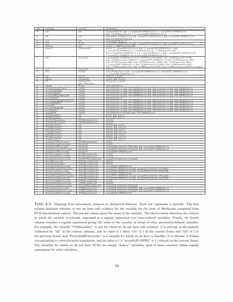
SE? variable context definition

0 clo nil !actualVEL(0) && ( actualLIP-OPEN(0)=0 ‖ ( actualTT-OPEN(0)=0&& !(TTPhone(0)=L) ) ‖ ( actualTB-OPEN(0)=0 ))

0 hh nil actualLIP-OPEN(0)>2 && actualTT-OPEN(0)>2 && actualTB-OPEN(0)>2&& actualGLOT(0)=2

0 voi nil actualGLOT(0)=1

0 stri Fr(0) actualTT-OPEN(0)=1 && ( actualTT-LOC(0)=1 && actualTT-LOC(0)=2 )

1 Silence nil clo(0) ‖ TBPhone(0)=SIL

1 Sonor !Silence(0) hh(0) ‖ ( actualGLOT(0)=1 && (( actualLIP-OPEN(0)>1 &&( actualTT-OPEN(0)>1 ‖ TTPhone(0)=L ‖ TTPhone(0)=EL )&& actualTB-OPEN(0)>1 ) ‖ ( actualVEL(0)=1 && ( actualLIP-OPEN(0)=0‖ actualTT-OPEN(0)=0 ‖ actualTB-OPEN(0)=0 ))))

1 SC Sonor(0) ((actualLIP-OPEN(0)<3 && !(LIPPhone(0)=EM) && !(LIPPhone(0)=UW)&& !(LIPPhone(0)=OW2)) ‖ (actualTT-OPEN(0)<3 && !(TTPhone(0)=EN)&& !(TTPhone(0)=ER) && !(TTPhone(0)=AXR) && !(TTPhone(0)=EL))‖ (actualTB-OPEN(0)<3 && !(TBPhone(0)=AXR) && !(TBPhone(0)=EL)&& !(TBPhone(0)=IY) && !(TBPhone(0)=UW) && !(TBPhone(0)=OW2))) ‖ hh(0)

0 syl Sonor(0) !SC(0)

0 NC SC(0) actualVEL(0)=1 && ( actualLIP-OPEN(0)=0 ‖ actualTT-OPEN(0)=0‖ actualTB-OPEN(0)=0 )

0 LG SC(0) !NC(0) ‖ hh(0)

1 Stops !Sonor(0) clo(0) && !clo(1)

0 Fr !Silence(0) !Stops(0) ‖ hh(0)&& !Sonor(0)

0 StriFr Fr(0) TT-LOC(0)=1

0 actualAA AY1 AO syl(0) TT-LOC(0)=1 && TT-OPEN(0)=5 && TB-LOC(0)=3 && TB-OPEN(0)=3

0 actualAE AW1 syl(0) TT-LOC(0)=1 && TT-OPEN(0)=5 && TB-LOC(0)=1 && TB-OPEN(0)=5

0 actualAH AX syl(0) TT-LOC(0)=1 && TT-OPEN(0)=4 && TB-LOC(0)=2 && TB-OPEN(0)=4

0 actualAW2 OW1 UH syl(0) TT-LOC(0)=2 && TT-OPEN(0)=5 && TB-LOC(0)=2 && TB-OPEN(0)=3

0 actualAXR syl(0) TT-LOC(0)=3

0 actualAY2 IH EY2 OY2 syl(0) TT-LOC(0)=1 && TT-OPEN(0)=3 && TB-LOC(0)=0 && TB-OPEN(0)=3

0 actualEH EY1 syl(0) TT-LOC(0)=1 && TT-OPEN(0)=4 && TB-LOC(0)=0 && TB-OPEN(0)=4

0 actualIY syl(0) TT-LOC(0)=1 && TT-OPEN(0)=3 && TB-LOC(0)=0 && TB-OPEN(0)=2

0 actualOW2 UW syl(0) TT-LOC(0)=2 && TT-OPEN(0)=5 && TB-LOC(0)=1 && TB-OPEN(0)=2

0 actualOY1 syl(0) TT-LOC(0)=1 && TT-OPEN(0)=5 && TB-LOC(0)=2 && TB-OPEN(0)=3

0 actualDX SC(0) TT-LOC(0)=TT ALV && TT-OPEN(0)=2

0 FrVBoundary nil Fr(0) && syl(1)

0 VFrBoundary nil Fr(0) && syl(-1)

0 StriFrVBoundary FrVBoundary(0) stri(0)

0 VStriFrBoundary VFrBoundary(0) stri(0)

0 SCVBoundary nil SC(0) && syl(1)

0 VSCBoundary nil SC(0) && syl(-1)

0 NCVBoundary nil NC(0) && syl(1)

0 VNCBoundary nil NC(0) && syl(-1)

0 LGVBoundary nil LG(0) && syl(1)

0 VLGBoundary nil LG(0) && syl(-1)

0 VStBoundary nil clo(0) && syl(-1)

1 AspirationPreVocalic FrVBoundary(0) hh(0)

1 StopVoicingPrevocalic Stops(0) voi(0)

1 StopVelarPrevocalic Stops(0) actualTB-LOC(0)=TB VEL && actualTB-OPEN(0)=0

1 StopAlveolarPrevocalic Stops(0) actualTT-LOC(0)=TT ALV && actualTT-OPEN(0)=0

1 StopLabialPrevocalic Stops(0) actualLIP-OPEN(0)=0

1 FricVoicingPrevocalic FrVBoundary(0) voi(0)

1 FricStridentPrevocalic FrVBoundary(0) stri(0)

1 FricAnteriorPrevocalic StriFrVBoundary(0) actualTT-LOC(0)=TT ALV

1 NasalPrevocalic SCVBoundary(0) NC(0)

1 NasalPostvocalic VSCBoundary(0) NC(0)

1 NasalLabialPrevocalic NCVBoundary(0) actualLIP-OPEN(0)=0

1 NasalAlveolarPrevocalic NCVBoundary(0) actualTT-OPEN(0)=0 && actualTT-LOC(0)=TT ALV

1 NasalVelarPrevocalic NCVBoundary(0) actualTB-OPEN(0)=0 && actualTB-LOC(0)=TB VEL

1 NasalLabialPostvocalic VNCBoundary(0) actualLIP-OPEN(0)=0

1 NasalAlveolarPostvocalic VNCBoundary(0) actualTT-OPEN(0)=0 && actualTT-LOC(0)=TT ALV

1 NasalVelarPostvocalic VNCBoundary(0) actualTB-OPEN(0)=0 && actualTB-LOC(0)=TB VEL

1 FricVoicingPostvocalic VFrBoundary(0) voi(0)

1 FricStridentPostvocalic VFrBoundary(0) stri(0)

1 FricAnteriorPostvocalic VStriFrBoundary(0) actualTT-LOC(0)=TT ALV

1 StopVelarPostvocalic VStBoundary(0) actualTB-LOC(0)=TB VEL && actualTB-OPEN(0)=0

1 StopAlveolarPostvocalic VStBoundary(0) actualTT-LOC(0)=TT ALV && actualTT-OPEN(0)=0

1 StopLabialPostvocalic VStBoundary(0) actualLIP-OPEN(0)=0

Table A.3: Mapping from articulatory features to distinctive features. Each row represents a variable. The first

column indicates whether or not we have soft evidence for the variable (in the form of likelihoods computed from

SVM discriminant values). The second column gives the name of the variable. The third column describes the context

in which the variable is relevant, expressed as a regular expression over time-indexed variables. Finally, the fourth

column contains a regular expression giving the value of the variable in terms of other previously-defined variables.

For example, the variable “VStBoundary” is one for which we do not have soft evidence, it is relevant in all contexts

(indicated by “nil” in the context column), and its value is 1 when “clo” is 1 in the current frame and “syl” is 1 in

the previous frame; and “FricLabialPostvocalic” is a variable for which we do have a classifier, it is relevant in frames

corresponding to vowel-fricative boundaries, and its value is 1 if “actualLIP-OPEN” is 1 (critical) in the current frame.

The variables for which we do not have SVMs are simply “helper” variables, used to more concisely define regular

expressions for other variables.

79

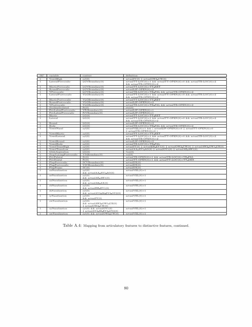
SE? variable context definition

1 VowelHigh syl(0) actualIY(0) ‖ actualOW2 UW(0)

1 LateralPrevocalic LGVBoundary(0) actualTT-LOC(0)=1 && actualTT-OPEN(0)=0 && actualTB-LOC(0)=2&& actualTB-OPEN(0)=2

1 RhoticPrevocalic LGVBoundary(0) actualTT-LOC(0)=TT RET

1 RoundPrevocalic LGVBoundary(0) actualLIP-OPEN(0)=2

1 YPrevocalic LGVBoundary(0) actualTB-LOC(0)=TB PAL && actualTB-OPEN(0)=2

1 LateralPostvocalic VLGBoundary(0) actualTT-LOC(0)=1 && actualTT-OPEN(0)=0 && actualTB-LOC(0)=2&& actualTB-OPEN(0)=2

1 RhoticPostvocalic VLGBoundary(0) actualTT-LOC(0)=TT RET

1 RoundPostvocalic VLGBoundary(0) actualLIP-OPEN(0)=2

1 YPostvocalic VLGBoundary(0) actualTB-LOC(0)=TB PAL && actualTB-OPEN(0)=2

1 StridentIsolated Fr(0) stri(0)

1 FricLabialPostvocalic VFrBoundary(0) actualLIP-OPEN(0)=1

1 FricLabialPrevocalic FrVBoundary(0) actualLIP-OPEN(0)=1

1 Rhotic LG(0) actualTT-LOC(0)=TT RET

1 Lateral LG(0) actualTT-LOC(0)=1 && actualTT-OPEN(0)=0 && actualTB-LOC(0)=2&& actualTB-OPEN(0)=2

1 Round LG(0) actualLIP-OPEN(0)=2

1 Body LG(0) actualTB-LOC(0)=TB PAL && actualTB-OPEN(0)=2

1 VowelNasal syl(0) actualVEL(0)=1 && ( actualLIP-OPEN(0)=0 ‖ actualTT-OPEN(0)=0‖ actualTB-OPEN(0)=0 )

1 VowelRhotic syl(0) actualTT-LOC(0)=TT RET

1 VowelLateral syl(0) actualTT-LOC(0)=1 && actualTT-OPEN(0)=0 && actualTB-LOC(0)=2&& actualTB-OPEN(0)=2

1 VowelRound syl(0) actualLIP-OPEN(0)=2

1 VowelBody syl(0) actualTB-LOC(0)=TB PAL

1 VowelTenseHigh syl(0) actualIY(0) ‖ actualEH EY1(0) ‖ actualOW2 UW(0) ‖ actualAW2 OW1 UH(0)

1 VowelTenseLow syl(0) actualAA AY1 AO(0) ‖ actualOY1(0) ‖ actualAE AW1(0)

1 GlideAspiration LG(0) !voi(0)

1 StopVoicingPostvocalic VStBoundary(0) voi(0)

1 FricPalatal Fr(0) actualTB-OPEN(0)=1 && actualTB-LOC(0)=TB PAL

1 FricDental Fr(0) actualTT-OPEN(0)=1 && actualTT-LOC(0)=TT DEN

1 FlapPrevocalic SCVBoundary(0) actualDX(0)

1 FlapPostvocalic VSCBoundary(0) actualDX(0)

1 FlapFrame SC(0) actualDX(0)

1 aaNasalization syl(0) actualVEL(0)=1&& actualAA AY1 AO(0)

1 aeNasalization syl(0) actualVEL(0)=1&& actualAE AW1(0)

1 axNasalization syl(0) actualVEL(0)=1&& actualAH AX(0)

1 ehNasalization syl(0) actualVEL(0)=1&& actualEH EY1(0)

1 ihNasalization syl(0) actualVEL(0)=1&& actualAY2 IH EY2 OY2(0)

1 iyNasalization syl(0) actualVEL(0)=1&& actualIY(0)

1 owNasalization syl(0) actualVEL(0)=1&& actualAW2 OW1 UH(0)‖ actualOW2 UW(0)

1 oyNasalization syl(0) && actualOY1(0) actualVEL(0)=1‖ actualAY2 IH EY2 OY2(0)

1 uwNasalization syl(0) && actualOW2 UW(0) actualVEL(0)=1

Table A.4: Mapping from articulatory features to distinctive features, continued.

80

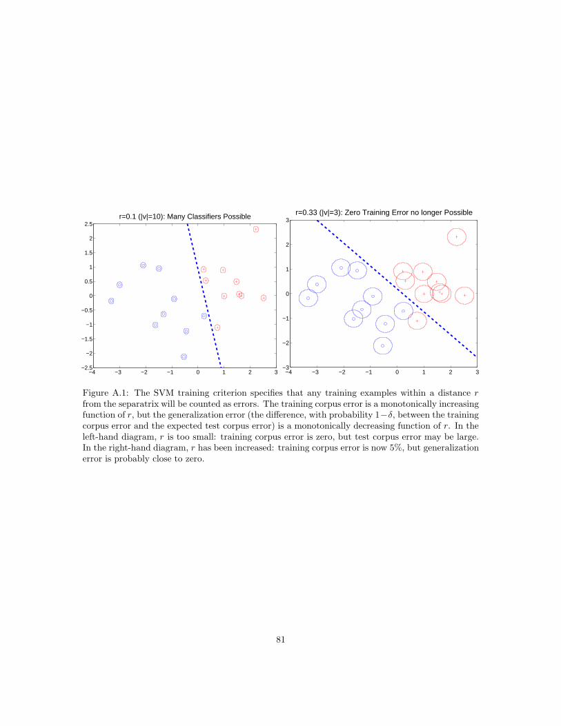
−4 −3 −2 −1 0 1 2 3−2.5

−2

−1.5

−1

−0.5

0

0.5

1

1.5

2

2.5r=0.1 (|v|=10): Many Classifiers Possible

−4 −3 −2 −1 0 1 2 3−3

−2

−1

0

1

2

3r=0.33 (|v|=3): Zero Training Error no longer Possible

Figure A.1: The SVM training criterion specifies that any training examples within a distance rfrom the separatrix will be counted as errors. The training corpus error is a monotonically increasingfunction of r, but the generalization error (the difference, with probability 1−δ, between the trainingcorpus error and the expected test corpus error) is a monotonically decreasing function of r. In theleft-hand diagram, r is too small: training corpus error is zero, but test corpus error may be large.In the right-hand diagram, r has been increased: training corpus error is now 5%, but generalizationerror is probably close to zero.

81

Bibliography

[1] Jont B. Allen. How do humans process and recognize speech? IEEE Trans. Speech and AudioProcessing, 2(4):567–577, Oct 1994.

[2] Jont B. Allen. Harvey Fletcher’s role in the creation of communication acoustics. Journal ofthe Acoustical Society of America, 99:1825–1839, 1996.

[3] Jont B. Allen. Articulation and intelligibility. (unpublished manuscript), 2003.

[4] Abeer Alwan, Shrikanth Narayanan, and Katherine Haker. Towards articulatory-acousticmodels of liquid approximants based on MRI and EPG data. Part II: The rhotics. J. Acoust.Soc. Am, 101(2):1078–1089, 1997.

[5] Abeer A. H. Alwan. Modeling Speech Perception in Noise: the Stop Consonants as a CaseStudy. PhD thesis, MIT, Cambridge, MA, February 1992.

[6] James Baker. The dragon system — an overview. IEEE Trans. Acoustics, Speech, and SignalProcessing, 23:24–29, 1975.

[7] Madeleine Bates. The use of syntax in a speech understanding system. IEEE Trans. Acoustics,Speech, and Signal Processing, 23(1):112–117, 1975.

[8] Alexander Bell. Visible Speech: The Science of the Universal Alphabetic. London, 1876.

[9] Y. Bengio, R. De Mori, G. Flammia, and R. Kompe. Global optimization of a neural network- hidden markov model hybrid. IEEE Trans. Neural Networks, 3(2):252–259, 1992.

[10] Y. Bengio, R. De Mori, G. Flammia, and R. Kompe. Phonetically motivated acoustic parame-ters for continuous speech recognition using artificial neural networks. Speech Communication,11(2-3):261–271, 1992.

[11] Jose R. Benki. Analysis of english nonsense syllable recognition in noise. Phonetica, 60:129–157, 2003.

[12] J. Bilmes, G. Zweig, T. Richardson, K. Filali, K. Livescu, P. Xu, K. Jackson, Y. Brandman,E. Sandness, E. Holtz, J. Torres, and B. Byrne. Discriminatively structured graphical modelsfor speech recognition. Technical report, Johns Hopkins CLSP Summer Workshop, 2001.

[13] Jeff Bilmes. Graphical models and automatic speech recognition. Technical Report UWEETR-2001-0005, University of Washington Dept. of Electrical Engineering, 2001.

[14] Jeff Bilmes. On soft evidence in Bayesian networks. Technical Report UWEETR-2004-0016,U. Washington Dept. of Electrical Engineering, 2004.

[15] Jeff Bilmes, Nelson Morgan, Su-Lin Wu, and Herve Bourlard. Stochastic perceptual speechmodels with durational dependence. In Proc. ICASSP, pages 1301–1304, 1996.

82

[16] Jeff Bilmes and Geoffrey Zweig. The Graphical Models Toolkit: An open source softwaresystem for speech and time-series processing. In Proc. ICASSP, 2002.

[17] Frederic Bimbot, Gerard Chollet, and Jean-Pierre Tubach. TDNNs for phonetic featuresextraction: A visual exploration. In Proc. ICASSP, pages 73–76, 1991.

[18] Nabil Bitar and Carol Espy-Wilson. A knowledge-based signal representation for speech recog-nition. In Proc. ICASSP, pages 29–32, 1996.

[19] Sheila E. Blumstein and Kenneth N. Stevens. Acoustic invariance in speech production: Ev-idence from measurements of the spectral characteristics of stop consonants. Journal of theAcoustical Society of America, 66(4):1001–1017, October 1979.

[20] Arthur Boothroyd, Bethany Mulhearn, Juan Gong, and Jodi Ostroff. Effects of spectralsmearing on phoneme and word recognition. Journal of the Acoustical Society of America,100(3):1807–1818, 1996.

[21] H. Bourlard and N. Morgan. Connectionist Speech Recognition: A Hybrid Approach. KluwerAcademic Publishers, Boston, MA, 1994.

[22] H. Bourlard, N. Morgan, C. Wooters, and S. Renals. CDNN: A context-dependent neuralnetwork for continuous speech recognition. In Proc. ICASSP, pages 349–352, San Francisco,1992.

[23] A. S. Bregman. Auditory Scene Analysis. MIT Press, 1990.

[24] Catherine P. Browman and Louis Goldstein. Articulatory phonology: An overview. Phonetica,49:155–180, 1992.

[25] C.J.C. Burges. A tutorial on support vector machines for pattern recognition. KnowledgeDiscovery and Data Mining, 2(2), 1998.

[26] Robert P. Carlyon and Shihab Shamma. An account of monaural phase sensitivity. Journalof the Acoustical Society of America, 114(1):333–348, 2003.

[27] Julie Carson-Berndsen. Time Map Phonology: Finite State Models and Event Logics in SpeechRecognition. Kluwer Academic Publishers, 1999.

[28] Christophe Cerisara and Dominique Fohr. Multi-band automatic speech recognition. Computerspeech and language, 15:151–174, 2001.

[29] Chih-Chung Chang and Chih-Jen Lin. LIBSVM: A library for support vector machines. Tech-nical report, National Taiwan University, 2004.

[30] Shuangyu Chang, Steven Greenberg, and Mirjam Wester. An elitist approach to articulatory-acoustic feature classification. In Proc. EUROSPEECH, 2001.

[31] Ken Chen and Mark Hasegawa-Johnson. How prosody improves word recognition. In ISCAInternat. Conf. Speech Prosody, Nara, Japan, 2004.

[32] Ken Chen, Mark Hasegawa-Johnson, Aaron Cohen, Sarah Borys, Sung-Suk Kim, JenniferCole, and Jeung-Yoon Choi. Prosody dependent speech recognition on radio news. IEEETrans. Speech and Audio Processing, in press.

[33] Ken Chen, Mark Hasegawa-Johnson, and Sung-Suk Kim. An intonational phrase boundaryand pitch accent dependent speech recognizer. In International Conference on Systems, Cy-bernetics, and Intelligence (SCI), Orlando, FL, 2003.

83

[34] Marilyn Chen. Nasal landmark detection. In Proc. ICSLP, pages 636–639, 2000.

[35] N. Chomsky and M. Halle. The Sound Pattern of English. Harper and Row, New York, NY,1968.

[36] G. N. Clements. The geometry of phonological features. Phonology Yearbook, 2:223–250, 1985.

[37] P. S. Cohen and R. L. Mercer. Phonological component of an automatic speech recognizer. InRaj Reddy, editor, Speech Recognition, pages 290–308. Academic Press, New York, 1975.

[38] Jennifer Cole, Hansook Choi, Heejin Kim, and Mark Hasegawa-Johnson. The effect of accenton the acoustic cues to stop voicing in radio news speech. In International Conference onPhonetic Sciences, 2003.

[39] Khalid Daoudi, Dominique Fohr, and Christophe Antoine. Dynamic bayesian networks formulti-band automatic speech recognition. Computer Speech and Language, 17(2-3):263–285,2003.

[40] Steven Davis and Paul Mermelstein. Comparison of parametric representations for monosyl-labic word recognition in continuously spoken sentences. Trans. ASSP, ASSP-28(4):357–366,August 1980.

[41] Pierre C. Delattre, Alvin M. Liberman, and Franklin S. Cooper. Acoustic loci and transitionalcues for consonants. Journal of the Acoustical Society of America, 27(4):769–773, July 1955.

[42] Bertrand Delgutte and Nelson Y.S. Kiang. Speech coding in the auditory nerve: IV. Soundswith consonant-like dynamic characteristics. Journal of the Acoustical Society of America,75:897–907, 1984.

[43] Gary S. Dell. The retrieval of phonological forms in production: Tests of predictions from aconnectionist model. In W. Marslen-Wilson, editor, Lexical Representation and Process, pages136–166. MIT Press, Cambridge, MA, 1992.

[44] A. P. Dempster, N. M. Laird, and D. B. Rubin. Maximum likelihood from incomplete datavia the EM algorithm. Journal of the Royal Statistical Society, 39:1–38, 1977.

[45] L. Deng and K. Erler. Hidden markov model representation of quantized articulatory featuresfor speech recognition. Computer Speech and Language, 7(3):265–282, 1993.

[46] Li Deng, Gordon Ramsay, and Don Sun. Production models as a structural basis for automaticspeech recognition. Speech Communication, 33:93–111, 1997.

[47] Om Deshmukh and Carol Espy-Wilson. A measure of periodicity and aperiodicity in speech.In Proc. ICASSP, pages 448–451, Hong Kong, 2003.

[48] Carol Espy-Wilson. A feature-based semi-vowel recognition system. Journal of the AcousticalSociety of America, 96(1):65–72, July 1994.

[49] Gunnar Fant. Acoustic Theory of Speech Production. Mouton and Co., The Hague, 1960.

[50] H. Fletcher. Speech and Hearing in Communication. van Nostrand, Princeton, NJ, 1953.

[51] Eric Fosler-Lussier. Contextual word and syllable pronunciation models. In IEEE Workshopon Automatic Speech Recognition and Understanding (ASRU), 1999.

[52] Qian-Jie Fu and Robert V. Shannon. Recognition of spectrally degraded speech in noise withnonlinear amplitude mapping. In Proc. ICASSP, Phoenix, AZ, 1999.

84

[53] Lai-Wo Fung and King-Sun Fu. Stochastic syntactic decoding for pattern classification. IEEETransactions on Computers, 23(1):662–667, 1975.

[54] Sadaoki Furui. On the role of spectral transition for speech perception. Journal of the Acous-tical Society of America, 80(4):1016–1025, 1983.

[55] Z. Ghahramani and M. Jordan. Factorial hidden Markov models. Machine Learning, 29:245–273, 1997.

[56] J. R. Glass and V. W. Zue. Multi-level acoustic segmentation of continuous speech. In Proc.ICASSP, New York, NY, April 1988.

[57] J.J. Godfrey, E.C. Holliman, and J. McDaniel. SWITCHBOARD: telephone speech corpus forresearch and development. In Proc. ICASSP, pages 517–520, 1992.

[58] John A. Goldsmith. Tone melodies and the autosegment. In Proceedings of the 6th Conferenceon African Linguistics, Ohio State University Working Papers in Linguistics, pages 135–147,Columbus, OH, 1975. Ohio State University.

[59] S. Greenberg, H. Carvey, L. Hitchcock, and S. Chang. The phonetic patterning of sponta-neous american english discourse. In IEEE Workshop on Spontaneous Speech Processing andRecognition (SSPR), Tokyo, 2003.

[60] S. Greenberg, H. Carvey, L. Hitchcock, and S. Chang. Temporal properties of spontaneousspeech - a syllabic centric perspective. J. Phonetics, 31(3-4):465–485, July-October 2003.

[61] S. Greenberg, H.M. Carvey, and L. Hitchcock. The relation of stress accent to pronunciationvariation in spontaneous american english discourse. In Proc. ISCA Workshop on Prosody andSpeech Processing, 2002.

[62] S. Greenberg, S. Chang, and J. Hollenback. An introduction to the diagnostic evaluation of theswitchboard-corpus automatic speech recognition systems. In Proceedings of the NIST SpeechTranscription Workshop, College Park, MD, 2000.

[63] S. Greenberg, J. Hollenback, and D. Ellis. Insights into spoken language gleaned from phonetictranscription of the Switchboard corpus. In Proc. ICSLP, 1996.

[64] Steven Greenberg. Recognition in a new key — towards a science of spoken language. In Proc.ICASSP, pages 1041–1045, Seattle, 1998.

[65] Steven Greenberg. Speaking in shorthand - a syllable-centric perspective for understandingpronunciation variation. Speech Communication, 29:159–176, 1999.

[66] Steven Greenberg. Pronunciation variation is key to understanding spoken language. InInternational Conference on Phonetic Sciences, pages 219–222, 2003.

[67] Steven Greenberg. Strategies for automatic multi-tier annotation of spoken language corpora.In Proc. EUROSPEECH, 2003.

[68] Steven Greenberg. A multi-tier framework for understanding spoken language. In S. Green-berg and W.A. Ainsworth, editors, Listening to Speech: An Auditory Perspective. LawrenceErlbaum Associates, Mahwah, NJ, 2005.

[69] Frank H. Guenther and Marin N. Gjaja. The perceptual magnet effect as an emergent propertyof neural map formation. Journal of the Acoustical Society of America, 100:1111–1121, 1996.

85

[70] Andrew K. Halberstadt. Heterogeneous Acoustic Measurements and Multiple Classifiers forSpeech Recognition. PhD thesis, MIT, Cambridge, MA, Nov. 1998.

[71] Andrew K. Halberstadt and James R. Glass. Heterogeneous acoustic measurements for pho-netic classification. In Proc. EUROSPEECH, pages 401–404, 1997.

[72] Andrew K. Halberstadt and James R. Glass. Heterogeneous measurements and multiple clas-sifiers for speech recognition. In Proc. ICSLP, Sydney, Australia, Nov. 1998.

[73] Trevor Hastie, Saharon Rosset, Rob Tibshirani, and Ji Zhu. The entire regularization path ofthe support vector machine. In NIPS, 2004.

[74] David Haussler. Decision theoretic generalizations of the PAC model for neural net and otherlearning applications. Information and Computation, 100:78–150, 1992.

[75] Hynek Hermansky. Perceptual linear predictive (plp) analysis of speech. Journal of the Acous-tical Society of America, 87(4):1738–1752, 1990.

[76] Hynek Hermansky and Sangita Sharma. Temporal patterns (TRAPS) in ASR of noisy speech.In Proc. ICASSP, Phoenix, 1999.

[77] James Hillenbrand, Laura A. Getty, Michael J. Clark, and Kimberlee Wheeler. Acousticcharacteristics of American English vowels. Journal of the Acoustical Society of America,97(5):3099–3111, May 1995.

[78] L. Hitchcock and S. Greenberg. Vowel height is intimately associated with stress accent inspontaneous american english discourse. In Proc. EUROSPEECH, pages 79–82, 2001.

[79] Andrew Wilson Howitt. Vowel landmark detection. In Proc. ICSLP, 2000.

[80] International Phonetic Association (IPA). International phonetic alphabet, 1993.

[81] Fumitada Itakura. Minimum prediction residual principle applied to speech recognition. IEEETrans. Acoustics, Speech, and Signal Processing, 23(1):67–72, 1975.

[82] R. Jakobson, G. Fant, and M. Halle. Preliminaries to speech analysis. Technical Report 13,MIT Acoustics Laboratory, 1952.

[83] Frederick Jelinek. Continuous speech recognition by statistical methods. Proc. IEEE,64(4):532–556, 1976.

[84] T. Joachims. Text categorization with support vector machines: Learning with many relevantfeatures. In Proc. of European Conference on Machine Learning, 1998.

[85] A. Juneja and C. Espy-Wilson. Significance of invariant acoustic cues in a probabilistic frame-work for landmark-based speech recognition. In From sound to sense: 50+ years of discoveriesin speech communication, pages C–151 to C–156, MIT, Cambridge MA, 2004.

[86] Amit Juneja. Speech recognition based on phonetic features and acoustic landmarks. PhDthesis, University of Maryland, 2004.

[87] Amit Juneja and Carol Espy-Wilson. A novel probabilistic framework for event-based speechrecognition. Journal of the Acoustical Society of America, 114(4(A)):2395, 2003.

[88] Amit Juneja and Carol Espy-Wilson. Speech segmentation using probabilistic phonetic fea-ture hierarchy and support vector machines. In Proc. Internat. Joint Conf. Neural Networks(IJCNN), Portland, OR, 2003.

86

[89] P. Jusczyk. Picking up regularities in the sound structure of the native language. In W. Strange,editor, Speech Perception and Linguistic Experience: Issues in Cross-Language Speech Re-search. York, Timotheum, MD, 1995.

[90] P. W. Jusczyk, A. D. Friederici, J. M. I. Wessels, V. Y. Svenkerud, and A. M. Jusczyk. Infants’sensitivity to the sound patterns of native language words. J. Mem. Lang., 32:402–420, 1993.

[91] Michael Kenstowicz. Phonology in Generative Grammar. Blackwell, Cambridge, Mas-sachusetts, 1994.

[92] S. J. Keyser and K. N. Stevens. Feature geometry and the vocal tract. Phonology, 11:207–236,1994.

[93] K. Kirchhoff, G. A. Fink, and G. Sagerer. Combining acoustic and articulatory feature infor-mation for robust speech recognition. Speech Communication, 37:303–319, 2002.

[94] Katrin Kirchhoff. Syllable-level desynchronisation of phonetic features for speech recognition.In Proc. ICSLP, 1996.

[95] Katrin Kirchhoff. Combining articulatory and acoustic information for speech recognition innoisy and reverberant environments. In Proc. ICSLP, 1998.

[96] Katrin Kirchhoff, G. Fink, and G. Sagerer. Conversational speech recognition using acousticand articulatory input. In Proc. ICASSP, Istanbul, Turkey, 2000.

[97] Dennis H. Klatt. Speech perception: a model of acoustic-phonetic analysis and lexical acess.J. Phonetics, 7:279–312, 1979.

[98] P. K. Kuhl, K. A. Williams, F. Lacerda, K. N. Stevens, and B. Linblom. Linguistic experiencealters phonetic perception in infants by 6 months of age. Science, 255:606–608, 1992.

[99] Peter Ladefoged. A Course in Phonetics. Harcourt Brace Jovanovich, Fort Worth, TX, 1982.

[100] John Lafferty, Andrew McCallum, and Fernando Pereira. Conditional random fields: Prob-abilistic models for segmenting and labeling sequence data. In International Conference onMachine Learning, 2001.

[101] Kai-Fu Lee. Context-dependent phonetic hidden Markov models for speaker-independent con-tinuous speech recognition. IEEE Trans. Acoustics, Speech, and Signal Processing, 38, 1990.

[102] S. Lee. Probabilistic segmentation for segment-based speech recognition. Master’s thesis,Massachusetts Institute of Technology, 1998.

[103] Ilse Lehiste and Gordon E. Peterson. Transitions, glides, and diphthongs. Journal of theAcoustical Society of America, 33(3):268–277, 1961.

[104] A. M. Liberman and I. G. Mattingly. The motor theory of speech perception revisited. Cog-nition, 21:1–36, 1985.

[105] Sharlene A. Liu. Landmark detection for distinctive feature-based speech recognition. Journalof the Acoustical Society of America, 100(5):3417–3430, Nov. 1996.

[106] Sharlene Anne Liu. Landmark detection for distinctive feature-based speech recognition. PhDthesis, MIT, Cambridge, MA, May 1995.

[107] Karen Livescu and James Glass. Feature-based pronunciation modeling for speech recognition.In Human Language Technology: Conference of the North American Chapter of the Associationfor Computational Linguistics (HLT/NAACL), 2004.

87

[108] Karen Livescu and James Glass. Feature-based pronunciation modeling with trainable asyn-chrony probabilities. In ICSLP, 2004.

[109] Jeri Logemann. Evaluation and Treatment of Swallowing Disorders (Second Edition). Pro-Ed,Inc., Austin, TX, 1998.

[110] L. Mangu, E. Brill, and A. Stolcke. Finding consensus in speech recognition: word errorminimization and other applications of confusion networks. Computer, Speech and Language,14(4):373–400, 2000.

[111] L. Mangu and M. Padmanabhan. Error corrective mechanisms for speech recognition. In Proc.ICASSP, pages 29–32, Salt Lake City, Utah, 2001.

[112] S. Y. Manuel, S. Shattuck-Hufnagel, K. N. Stevens, R. Carlson, and S. Hunnicutt. Studies ofvowel and consonant reduction. In Proc. ICSLP, pages 943–946, Banff, Alberta, 1992.

[113] Dominic Massaro. Speech Perception by Ear and Eye: A Paradigm for Psychological Inquiry.Erlbaum, Hillsdale, NJ, 1987.

[114] D. McAllaster, L. Gillick, F. Scattone, and M. Newman. Fabricating conversational speechdata with acoustic models: A program to examine model-data mismatch. In Proc. ICSLP,pages 1847–1850, 1998.

[115] Erik McDermott, Hitoshi Iwamida, Shigeru Katagiri, and Yoh’ichi Tohkura. Shift-tolerantlvq and hybrid lvq-hmm for phoneme recognition. In Readings in Speech Recognition, pages425–438. Morgan Kaufmann, San Mateo, CA, 1990.

[116] J. Mehler, P. W. Jusczyk, G. Lambertz, N. Halstead, J. Bertoncini, and C. Amiel-Tison. Aprecursor of language acquisition in young infants. Cognition, 29:143–178, 1988.

[117] Nima Mesgarani, Malcolm Slaney, and Shihab A. Shamma. Speech discrimination based onmultiscale spectrotemporal features. In Proc. ICASSP, 2004.

[118] G. A. Miller and P. E. Nicely. Analysis of perceptual confusions among some English conso-nants. Journal of the Acoustical Society of America, 27:338–352, 1955.

[119] George A. Miller. Decision units in the perception of speech. IRE Transactions on InformationTheory, pages 81–83, 1962.

[120] George A. Miller, George A. Heise, and William Lichten. The intelligibility of speech as afunction of the context of the test materials. Journal of Experimental Psychology, 41:329–335,1951.

[121] George A. Miller and Stephen Isard. Some perceptual consequences of linguistic rules. Journalof Verbal Learning and Verbal Behavior, 2:217–228, 1963.

[122] M.I. Miller and M.B. Sachs. Representation of stop consonants in the discharge patterns ofauditory-nerve fibers. Journal of the Acoustical Society of America, 74:502–517, 1983.

[123] Hosung Nam and Elliot Saltzman. A competitive, coupled oscillator model of syllable structure.In International Conference on Phonetic Sciences, 2003.

[124] Shrikanth S. Narayanan, Abeer A. Alwan, and Katherine Haker. Towards articulatory-acousticmodels of liquid approximants based on MRI and EPG data. Part I: The laterals. J. Acoust.Soc. Am, 101(2):1064–1077, 1997.

88

[125] Bonnie Nash-Webber. Semantic support for a speech understanding system. IEEE Trans.Acoustics, Speech, and Signal Processing, 23(1):124–129, 1975.

[126] Partha Niyogi and Chris Burges. Detecting and interpreting acoustic features by supportvector machines. Technical Report 2002-02, University of Chicago Computer Science Dept,2002.

[127] Partha Niyogi, Chris Burges, and Padma Ramesh. Distinctive feature detection using supportvector machines. In Proc. ICASSP, Phoenix, AZ, 1999.

[128] Partha Niyogi and Padma Ramesh. Incorporating voice onset time to improve letter recognitionaccuracies. In Proc. ICASSP, pages 13–16, 1998.

[129] Harriet Nock and Mari Ostendorf. Parameter reduction schemes for loosely coupled hmms.Computer Speech and Language, 17(2-3):233–262, 2003.

[130] Harriet J. Nock and Steven J. Young. Modelling asynchrony in automatic speech recognitionusing loosely coupled hidden Markov models. Cognitive Science, 26(3):283–301, 2002.

[131] Zaki B. Nossair and Stephen A. Zahorian. Dynamic spectral shape features as acoustic corre-lates for initial stop consonants. Journal of the Acoustical Society of America, 89(6):2978–2991,June 1991.

[132] King Sejong of Joseon. Hunmin Jeongeum. 1446.

[133] M. Kamal Omar and Mark Hasegawa-Johnson. Approximately independent factors of speechusing non-linear symplectic transformation. IEEE Trans. Speech and Audio Processing,11(6):660–671, 2003.

[134] M. Kamal Omar and Mark Hasegawa-Johnson. Model enforcement: A unified feature trans-formation framework for classification and recognition. IEEE Trans. Signal Processing, 52(10),2004.

[135] M. Kamal Omar, Mark Hasegawa-Johnson, and Stephen E. Levinson. Gaussian mixture mod-els of phonetic boundaries for speech recognition. In IEEE Workshop on Automatic SpeechRecognition and Understanding (ASRU), 2001.

[136] B. T. Oshika, V. W. Zue, R. V. Weeks, H. Neu, and J. Aurbach. The role of phonologicalrules in speech understanding research. IEEE Trans. Acoustics, Speech, and Signal Processing,23(1):104–112, February 1975.

[137] Mari Ostendorf, Vassilios V. Digilakis, and Owen A. Kimball. From HMM’s to segment models:A unified view of stochastic modeling for speech recognition. IEEE Trans. Speech and AudioProcessing, 4(5):360–378, 1996.

[138] Gordon E. Peterson and Harold L. Barney. Control methods used in a study of vowels. Journalof the Acoustical Society of America, 24(2):175–184, March 1952.

[139] Tarun Pruthi and Carol Y. Espy-Wilson. Acoustic parameters for automatic detection of nasalmanner. Speech Communication, 43(3):225–240, 2004.

[140] Matt Richardson, Jeff Bilmes, and Chris Diorio. Hidden-articulator markov models: perfor-mance improvements and robustness to noise. In Proc. ICSLP, 2000.

[141] Michael D. Riley and Andrej Ljolje. Automatic generation of detailed pronunciation lexicons.In Chin-Hui Lee, Frank K. Soong, and Kuldip K. Paliwal, editors, Automatic Speech andSpeaker Recognition: Advanced Topics, pages 285–302. Kluwer, Boston, 1996.

89

[142] Kourosh Saberi and David R. Perrott. Cognitive restoration of reversed speech. Nature,398(6730):760, April 1996.

[143] Elliot L. Saltzman and Kevin J. Munhall. A dynamical approach to gestural patterning inspeech production. Haskins Laboratories Status Report on Speech Research, SR-99/100:38–68,1989.

[144] Lawrence K. Saul, Mazin G. Rahim, and Jont B. Allen. A statistical model for robust inte-gration of narrowband cues in speech. Computer speech and language, 15(2):175–194, 2001.

[145] G. Schwartz. Estimating the dimension of a model. The Annals of Statistics, 5(2):461–464,1978.

[146] R.V. Shannon, F. Zeng, V. Kamath, J. Wygonski, and M. Ekelid. Speech recognition withprimarily temporal cues. Science, 270:303–304, 1995.

[147] Anu Sharma and Michael F. Dorman. Exploration of the perceptual magnet effect using themismatch negativity auditory evoked potential. Journal of the Acoustical Society of America,104:511–517, 1998.

[148] Wai Ting Siok, Zhen Jin, P. Fletcher, and Li Hai Tan. Distinct brain regions associated withsyllable and phoneme. Human Brain Mapping, 18(3):201–7, 2003.

[149] N. Smith and M.J.F. Gales. Using SVMs and discriminative models for speech recognition. InProceedings of ICASSP, 2002.

[150] K. N. Stevens. Evidence for the role of acoustic boundaries in the perception of speech sounds.In Victoria A. Fromkin, editor, Phonetic Linguistics: Essays in Honor of Peter Ladefoged,pages 243–255. Academic Press, Orlando, Florida, 1985.

[151] K. N. Stevens and S. J. Keyser. Primary features and their enhancement in consonants.Language, 65(1):81–106, 1989.

[152] K. N. Stevens, S. J. Keyser, and H. Kawasaki. Toward a phonetic and phonological theoryof redundant features. In J. S. Perkell and D. H Klatt, editors, Invariance and Variability inSpeech Processes, pages 426–463. Lawrence Erlbaum Associates, Hillsdale, NJ US, 1986.

[153] K. N. Stevens, S. Y. Manuel, S. Shattuck-Hufnagel, and S. Liu. Implementation of a modelfor lexical access based on features. In Proc. ICSLP, volume 1, pages 499–502, Banff, Alberta,1992.

[154] Kenneth N. Stevens. Acoustic Phonetics. MIT Press, Cambridge, MA, 1999.

[155] Kenneth N. Stevens, Sheila E. Blumstein, Laura Glickman, Martha Burton, and KathleenKurowski. Acoustic and perceptual characteristics of voicing in fricatives and fricative clusters.Journal of the Acoustical Society of America, 91(5):2979–3000, May 1992.

[156] Kenneth N. Stevens and Arthur S. House. Development of a quantitative description of vowelarticulation. Journal of the Acoustical Society of America, 27(3):401–493, 1955.

[157] Helmer Strik and Catia Cucchiarini. Modeling pronunciation variation for ASR: A survey ofthe literature. Speech Communication, 29:225–246, 1999.

[158] Harvey M. Sussman, Helen A. McCaffrey, and Sandra A. Matthews. An investigation of locusequations as a source of relational invariance for stop place categorization. Journal of theAcoustical Society of America, 90(3):1309–1325, September 1991.

90

[159] Ming-Yi Tsai, Fu chiang Chou, and Lin shan Lee. Improved pronunciation modeling byproperly integrating better approaches for baseform generation, ranking and pruning. In ISCAWorkshop on Pronunciation Modeling and Lexical Access (PMLA), 2002.

[160] Vladimir Vapnik. Statistical Learning Theory. Wiley, New York, 1998.

[161] V. Venkataramani and W. Byrne. Lattice segmentation and support vector machines forlarge vocabulary continuous speech recognition. In IEEE Conference on Acoustics, Speech andSignal Processing, 2005. To Appear.

[162] Veera Venkataramani, Shantanu Chakrabartty, and William Byrne. Support vector machinesfor segmental minimum bayes risk decoding of continuous speech. In IEEE Workshop onAutomatic Speech Recognition and Understanding (ASRU), 2003.

[163] Dimitra Vergyri. Use of word level side information to improve speech recognition. In Proc.ICASSP, 2000.

[164] Lydia E. Volaitis and Joanne L. Miller. Phonetic prototypes: Influence of place of articulationand speaking rate on the internal structure of voicing categories. Journal of the AcousticalSociety of America, 92(2):723–735, August 1992.

[165] Alexander Waibel, Toshiyuki Hanazawa, Geoffrey Hinton, Kiyohiro Shikano, and Kevin J.Lang. Phoneme recognition using time-delay neural networks. Trans. Acoust. Speech Sig.Proc., 37:328–339, 1989.

[166] W. Wang, A. Stolcke, and M.P. Harper. The use of a linguistically motivated language modelin conversational speech recognition. In Proceedings of ICASSP, 2004.

[167] Richard M. Warren, Eric W. Healy, and Magdalene H. Chalikia. The vowel-sequency illusion:Intrasubject stability and intersubject agreement of syllabic forms. Journal of the AcousticalSociety of America, 100:2452–2461, 1996.

[168] Katrin Weber, Shajith Ikbal, Samy Bengio, and Herve Bourlard. Robust speech recognitionand feature extraction using HMM2. Computer Speech and Language, 17(2-3):195–211, 2003.

[169] Mitch Weintraub, Eric Fosler, Charles Galles, Yu-Hung Kao, Sanjeev Khudanpur, MuratSaraclar, and Steven Wegman. Automatic learning of word pronunciation from data: Finalreport. Technical Report WS96, Johns Hopkins University Center for Language and SpeechProcessing, 1996.

[170] Fuliang Weng, Andreas Stolcke, and Ananth Sankar. Efficient lattice representation and gen-eration. In Proc. ICSLP, pages 2531–2534, 1998.

[171] Mirjam Wester and Eric Fosler-Lussier. A comparison of data-derived and knowledge-basedmodeling of pronunciation variation. In Proc. ICSLP, 2000.

[172] Robert E. Wickesberg. Rapid inhibition in the cochlear nuclear complex of the chinchilla. J.Acoust. Soc. Am., 100:1691–1701, 1996.

[173] Robert E. Wickesberg and Hanna E. Stevens. Responses of auditory nerve fibers to trains ofclicks. Journal of the Acoustical Society of America, 103:1990–1999, 1998.

[174] A. A. Wrench and K. Richmond. Continuous speech recognition using articulatory data. InProc. ICSLP, 2000.

[175] H. Yu and A. Waibel. Integrating thumbnail features for speech recognition using conditionalexponential models. In Proc. ICASSP, pages 893–896, 2004.

91

[176] Yanli Zheng and Mark Hasegawa-Johnson. Formant tracking by mixture state particle filter.In Proc. ICASSP, 2004.

[177] Yanli Zheng and Mark Hasegawa-Johnson. Stop consonant classification by dynamic formanttrajector. In Proc. ICSLP, 2004.

[178] Victor Zue. The use of speech knowledge in automatic speech recognition. Proc. IEEE,73(11):1602–1615, November 1985.

[179] Geoffrey Zweig. Speech Recognition with Dynamic Bayesian Networks. PhD thesis, U. C.Berkeley, 1998.

92