Theoretical and Mathematical Physics, 163(2): 677–695 (2010)

LANGEVIN EQUATION OF A FLUID PARTICLE IN WALL-INDUCED

TURBULENCE

J. J. H. Brouwers∗

We derive the Langevin equation describing the stochastic process of fluid particle motion in wall-induced

turbulence (turbulent flow in pipes, channels, and boundary layers including the atmospheric surface layer).

The analysis is based on the asymptotic behavior at a large Reynolds number. We use the Lagrangian

Kolmogorov theory, recently derived asymptotic expressions for the spatial distribution of turbulent energy

dissipation, and also newly derived reciprocity relations analogous to the Onsager relations supplemented

with recent measurement results. The long-time limit of the derived Langevin equation yields the diffusion

equation for admixture dispersion in wall-induced turbulence.

Keywords: turbulence, dispersion, Langevin equation, Onsager reciprocity

1. Introduction

Fluid flow bounded by walls such as the earth’s surface or a pipe wall is often turbulent. Fluid velocitiesand pressures vary randomly with time and space. Despite many efforts over the past century, there is nogeneral mathematical description of the stochastic process of turbulence. The best that has been achieved isasymptotic descriptions of certain statistical parameters in the limit of large values of the Reynolds numberRe = u∗Lν−1, where u∗ is the shear velocity (u∗ =

√τ0/ρ, where τ0 is the mean shear stress exerted on

the wall by the fluid and ρ is the fluid density), ν is the fluid kinematic viscosity, and L is the externallength (pipe radius, channel half-width, turbulent boundary layer thickness along a wall or along the earth’ssurface).

Several asymptotic expressions applicable at Re � 1 have so far been derived, for example, Kol-mogorov’s renowned descriptions of the small scales of turbulence [1] and the logarithm law for the meanflow along a wall [2]. But the classical problem of calculating turbulent dispersion remains unsolved. Aproper theory exists only for the theoretical abstraction of homogeneous isotropic turbulence. It dates backto [3] written in 1921. But turbulence is an inhomogeneous anisotropic process. In all important cases ofturbulent flow, the fixed-point statistical means (i.e., Eulerian averages) of fluid velocities vary considerablyin space and direction.

A theory convincingly treating admixture dispersion in inhomogeneous anisotropic turbulence has notyet appeared. The standard approach is to use the Boussinesq hypothesis, which leads to a semiempiricalequation for turbulent dispersion [2]. The expressions for the diffusion coefficients in this equation areapproximate; they are based on a Reynolds analogy and are fitted to measurement results.

A more fundamental approach starts from a Langevin equation for the fluid particle velocity; thisapproach is analogous to the description of the Rayleigh particle in molecular dynamics [4]. An importantadvantage of this method is that it is consistent with the asymptotic structure of turbulent flow at a largeReynolds number. The equation can be made to match the inertial subrange limit of the Lagrangian version

∗Eindhoven University of Technology, Eindhoven, Netherlands, e-mail: J.J.H.Brouwers@tue.nl.

Prepared from an English manuscript submitted by the author; for the Russian version, see Teoreticheskaya i

Matematicheskaya Fizika, Vol. 163, No. 2, pp. 328–352, May, 2010. Original article submitted December 8, 2009.

0040-5779/10/1632-0677 c© 2010 Springer Science+Business Media, Inc. 677

of Kolmogorov’s similarity theory [5]. But the big problem concerns the form of the damping function in theLangevin equation. While the damping function is well established for homogeneous isotropic turbulence,a unique expression applicable to anisotropic inhomogeneous turbulence is lacking.

Here, we consider admixture dispersion in inhomogeneous anisotropic wall-induced turbulence. We usethe Langevin equation and derive an almost asymptotically exact description of the damping function. Weuse the Lagrangian Kolmogorov theory, recently derived asymptotic expressions for the spatial distributionof turbulent energy dissipation, and newly derived reciprocity relations analogous to the Onsager symmetryrelations. The long-time limit applied to the derived Langevin equation yields an almost exact version ofthe diffusion equation for admixture dispersion in wall-induced turbulence.

2. Langevin equation

Describing the stochastic process of turbulent motion of a fluid particle with the Langevin equationassumes that the fluid particle acceleration behaves as a δ-correlated process. The justification for applyingthis assumption to turbulence is that accelerations are governed by the small viscous scales, which obeyKolmogorov scaling [5]; this feature is apparently confirmed by experiment [6]. The correlation times ofparticle acceleration are related to those of velocity as Re−1/2. As Re increases, the stochastic processdescribing the velocity in large-scale turbulence is likely to resemble a Markov process more and more,and it can be modeled by a Langevin equation. The white-noise term in the equation can be describedin accordance with the inertial subrange limit of the Kolmogorov nonintermittent Lagrangian similaritytheory [5]. The Langevin equation relevant to stochastic turbulence then becomes [7]

dv′idt

= a′i(v

′, x) +√

C0ε(x) wi(t), i = 1, 2, 3, (1)

where v′ = v′(t) is the statistical fluctuation of the fluid particle velocity with respect to the Eulerian meanvelocity u0(x) evaluated at the particle position x = x(t). The velocity is related to the position by

dxi

dt= u0

i (x) + v′i. (2)

In (1), a′i = a′

i(v′, x) is the damping function, C0 is the universal Kolmogorov constant, ε = ε(x) is the

energy dissipation rate averaged at a fixed position, and wi(t) is Gaussian white noise of unit intensity.Equations (1) and (2) can be solved for various realizations of wi(t) with appropriate conditions at t = 0.The statistics of the velocity and position of a tagged fluid particle or passive fluid admixture can then beevaluated by averaging the resulting time records at fixed instants. The means thus obtained are denotedby an overbar. An alternative method for obtaining the same statistical information is to solve the Fokker–Planck equation for the joint probability of the particle velocity and position associated with Eqs. (1)and (2).

Describing particle velocity statistics with the Langevin equation relies on applying ordinary nonin-termittent Kolmogorov (K-41) theory. The intermittency effects are not taken into account in such anapproach. We could adopt a fractal model based on Kolmogorov’s refined similarity theory [8], but thestatistical means of the particle displacement, which determine the turbulent dispersion, change little inthis case [9], [10]. The intermittency effect is apparent at small (viscous) scales, not at the large (energetic)scales governing the stochastic process describing the velocity in turbulent flows at Re � 1 [11]. For thesereasons among others, a Langevin model based on K-41 theory is considered a reasonable approach formodeling dispersion.

678

To predict the statistics of particle velocities and positions using Eqs. (1) and (2), we need descriptionsof u0

i (x), ε(x), and a′i(v

′, x). Descriptions of the mean Eulerian velocity in wall-induced turbulence havebeen obtained theoretically and experimentally [2]. For the mean energy dissipation rate, we can use theasymptotic equality of energy dissipation and energy production [12]. What is unknown in the Langevinequation is the damping function a′

i(v′, x). The form of the damping function has been established only

for homogeneous isotropic turbulence [7], [13], [14]. A well-founded unique formulation of a′i(v

′, x) in thepractically relevant case of inhomogeneous wall-induced turbulence does not exist. We derive such a formulain the next section.

3. Spatial distribution of the damping function

The description of the statistics of particle velocities and positions using Eqs. (1) and (2) is La-grangian. Considerable progress has recently been made in the experimental and numerical determinationof the Lagrangian properties of turbulent flow [15]. The results tend to confirm the Lagrangian versionof Kolmogorov’s universal theory of small scales (see, e.g., [6]). As such, they support the correctness ofusing the forcing term in Langevin equation (1), which summarizes the effect of the small “viscous” scaleson velocity statistics for Re � 1. But the reported Lagrangian-based results are less useful for specifyingthe damping term, which significantly determines the statistical behavior of particle velocities and dis-placements. This behavior is governed by the large “energetic” scales of turbulence, whose structure isinhomogeneous and depends on the configuration in which the turbulent flow occurs. Lagrangian-basedstatistics can be used to determine the damping function if they encompass a region that is large enough tocapture the spatial dependence of the statistical parameters. Furthermore, in the present case, they shouldapply to configurations relevant to turbulence generated by mean flows along walls. In Sec. 8, we use thefew available results satisfying these criteria.

A more rewarding approach for obtaining information leading to a specification of the damping functionis to establish a connection with the more explored field of Eulerian (i.e., fixed-point) velocity statistics.This connection is obtained from the Eulerian interpretation of the Fokker–Planck equation associated withEqs. (1) and (2), also known as the well-mixed condition [16]. It yields a prescription for the probabilitydensity function of the fixed-point Eulerian velocity. The Eulerian version of the Fokker–Planck equationassociated with Eqs. (1) and (2) and appropriate for wall-induced turbulence is

− ∂

∂u′i

a′i(u

′, x2)p +12C0ε

∂2p

∂u′i∂u′

i

= u′2

∂p

∂x2, (3)

where p = p(u′) is the probability density of the fixed-point fluctuating (Eulerian) fluid velocity u. Here andhereafter, repeated indices imply summation. In formulating Eq. (3), we use the properties of wall-inducedturbulence that the Eulerian-based statistics are stationary (∂p/∂t = 0) and only vary with the distancex2 perpendicular to the wall. This is exactly true for developed turbulent flow in pipes and (almost) two-dimensional channels and is a good approximation for turbulent boundary layers along flat plates includingneutrally stratified atmospheric surface layers (see, e.g., [2]). While x2 is the coordinate perpendicular toboth the wall and the mean flow, the coordinates x1 and x3 are respectively taken parallel to both the meanflow and the wall and perpendicular to the mean flow and parallel to the wall. The mean flow in Eq. (2) isdescribed by

u0i (x) = u0

1(x2)δ1i, (4)

where δ1i is the Kronecker delta.

679

To specify the damping function a′i(v

′, x) in Langevin equation (1), we first focus our attention on theinertial sublayer, the region outside the viscous layer and where the mean flow u0

1(x2) can be described by thelogarithm law [2]. The inertial sublayer is the domain Re−1 � x2/L � 1, in practice, the domain 30 Re−1 �x2/L � 0.1. Below (see Sec. 7), we extend our results to the entire main section 30 Re−1 � x2/L ≤ 1.In the inertial sublayer, the statistical values of fluctuating velocities can be considered independent ofx2. Furthermore, an asymptotic analysis of the energy balance equations indicates that dissipation equalsproduction in the inertial sublayer [12]. This implies that in the inertial sublayer, ε behaves according to

ε = κ−1 u3∗

x2, Re−1 � x2

L� 1, (5)

where κ is Von Karman’s constant, κ ≈ 0.4. Meaningful expressions for p are obtained from Eq. (3) only ifboth the damping term and the diffusion term are retained under the limit process x2 → 0 appropriate forthe inertial sublayer. At the same time, p should become independent of x2 because the statistical valuesof fluctuating velocities are constant in the inertial sublayer. This requires that

a′i(u

′, x2) =a′

i(u′)

x2, (6)

and Eq. (3) then becomes

− ∂

∂u′i

a′i(u

′)p +12C0κ

−1u3∗

∂2p

∂u′i∂u′

i

= 0. (7)

Equation (6) specifies the spatial distribution of the damping function. It remains to specify its velocitydependence.

4. Gaussian velocities and linear damping

The next step is to assume that the single-point Eulerian velocities have a Gaussian distribution. Mea-surements indicate typical absolute values of skewness and kurtosis � 0.3 [17]–[19]. In these circumstances,a realistic approach is to use a Langevin model that leads to Gaussian Eulerian velocity statistics. Thisrequires that the function a′

i(u′) in (7) be linear in u′:

a′i(u

′) = −αiju′j. (8)

Experimental data indicate that Gaussianity is a reasonable assumption. Linear damping and Gaussianityof the Eulerian velocities can also be inferred from the correspondence between the considered stochas-tic processes describing velocity fluctuations and the stochastic processes describing closed nondissipativeHamiltonian systems known in theoretical physics. Below (see Sec. 6), we show that such a correspondenceexists if the inverse of the Kolmogorov constant is small.

5. Matching covariances

Well-mixing is accomplished by requiring that the solutions of Eqs. (7) and (8) comply with the valueof the covariance tensor σij = 〈u′

iu′j〉 of the Eulerian velocity field, which we assume to be known (angle

brackets denote ensemble means at fixed positions; because we treat stationary turbulence and implementergodicity, these means can be determined from time averaging at fixed positions). This requirement leads torelations between αij and σij . These can be obtained by substituting a general three-dimensional Gaussiandistribution function in Eq. (7) and equating like terms. It is simpler and more direct to multiply Eq. (7)by u′

mu′n, integrate over all values of u′, and integrate by parts, which yields

αnjσjm + αmjσjn = δmnC0κ−1u3

∗, (9)

680

where, we recall, repeated indices imply summation. For the type of turbulence under consideration,we can assume reflectional symmetry with respect to the x1x2 plane, i.e., particle velocities in the x3

direction are not correlated with those in the streamwise x1 and wall-normal x2 directions. This impliesα13 = α31 = α23 = α32 = 0. The solution of Eq. (9) then becomes

αij =12κ−1C0u

3∗(λij + b0γij), (10)

where λij = σ−1ij is the inverse of the covariance tensor,

λij =

d−1σ22 −d−1σ12 0

−d−1σ12 d−1σ11 0

0 0 σ−133

, d = σ11σ22 − σ2

12 > 0. (11)

We note that u′3 is not correlated with u′

1 and u′2. The tensor γij is defined as

γij =

−d−1σ12 d−1σ11 0

−d−1σ22 d−1σ12 0

0 0 0

. (12)

In Eq. (10), b0 is a constant whose value is unknown; it appears because we have five unknown valuesof αij and effectively four equations (see Eqs. (9)) as a result of applying the well-mixed condition. Thisreflects what is called the nonuniqueness problem: a full statistical specification of fixed-point Eulerianvelocities is insufficient for completely specifying the Langevin equation using the well-mixed condition [7].Equally, because of the phenomenon of convection of small scales by large scales, no relevant informationcan be obtained from time correlations of Eulerian-based velocities [20]. We now solve the nonuniquenessproblem by introducing a reciprocity requirement analogous to the Onsager reciprocity, simultaneouslyusing measurement results and direct numerical simulations (DNSs).

6. Reciprocity

We focus our attention on the random process describing fluctuations of fluid particles located at thedistance L0 from the wall at t = 0. We introduce dimensionless variables, marked with asterisks, as

x2 = L0x∗2, t = L0u

−1∗ t∗, v′i = u∗v

′i∗, α∗

ij = λ∗ij + b0γ

∗ij , (13)

where λ∗ij and γ∗

ij are defined according to (11) and (12) with σij replaced with σ∗ij = σij/u2

∗. ApplyingEq. (13) and dropping the asterisks, from Eqs. (1), (5), (6), (8), and (10), we obtain the dimensionlessLangevin equation

dv′idt

= −12C0κ

−1(λij + b0γij)v′jx2

+(

C0κ−1

x2

)1/2

wi(t), (14)

wheredx2

dt= v′2. (15)

The damping tensor consists of a symmetric part λij and an asymmetric part γij . The asymmetric partcauses the cross-correlation functions v′1(0)v′2(t) and v′2(0)v′1(t) to differ from each other; the overbar denotesaveraging at fixed times over many realizations of the Lagrangian variable, where each realization beginsat t = 0 with a random velocity value chosen in accordance with the Gaussian distribution of the Eulerian

681

velocity at the marked point x2 = 1. The difference between the two cross correlations depends on themagnitude of b0: the larger b0 is, the larger the difference. The Onsager reciprocity relation [21], [22] impliesthat the two correlations must be the same: b0 = 0. But the prerequisite for the reciprocity is Hamiltoniandynamics of the particles. Fluid particle dynamics are non-Hamiltonian because they undergo dissipationby viscosity. The viscosity effect appears at the small “viscous” scales of turbulence. The contribution ofthese scales to the velocity correlation functions vanishes as the value of the Reynolds number increases.More precisely, its effect shrinks to a discontinuity in the slope of the autocorrelation functions as t → 0(also see Fig. 1). Nevertheless, the dissipation effect in the energy equation for the turbulent flow does notvanish as Re → ∞ [11]. There is a continuous flow of energy from production at large scales to dissipation atsmall scales. This can be seen in the mean energy dissipation rate, whose magnitude equals κ−1u3

∗L−10 x−1

2

(see Eq. (5)). The total energy change as a function of the previously defined dimensionless time (seeEq. (13)) amounts to u2

∗κ−1tx−1

2 . Hence, a relative energy change ∆H/u2∗ of the order O(1) occurs over a

time period t of the order O(1).There is still a possibility to apply reciprocity to the turbulence problem to a certain degree because the

Kolmogorov constant in the Langevin equation has a relatively large value. For flow with a large Reynoldsnumber, the quantity C0 can be as large as 6 [14]. It can be seen from Eq. (14) that the time of randomvelocity fluctuations scales as C−1

0 and velocities decorrelate over a time C−10 . If we describe the solution

of the Langevin equation as an expansion in powers of C−10 , then the dissipation effect vanishes in the first

term. To consider this in more detail, we introduce the expansion parameter

ε1 = C−10 . (16)

With time and position scaled as

t = ε1t′, x2 = 1 + ε1x

′2, (17)

Langevin equation (14) becomes

dv′idt′

= −12κ−1(λij + b0γij)

v′j1 + ε1x′

2

+(

κ−1

1 + ε1x′2

)1/2

wi(t′), (18)

while (cf. Eq. (15))

x′2 =

∫ t′

0

v′2 dt. (19)

The total energy change with an error of the order O(ε21) becomes

∆H

u2∗

∼ ε1t′, (20)

where ∼ means asymptotically equal.We now consider the probability density and the correlation function of the particle velocity described

by Langevin equation (18). Representing the solution as an expansion in powers of ε1, we obtain thefirst term of such an expansion from Eq. (18) with ε1 = 0. As a solution, the Langevin equation thusobtained has an exponentially correlated Gaussian process [4], which, as is known, is used to describeclosed nondissipative systems [22]. Furthermore, the underlying fluid particle dynamics in the case ε1 = 0with t′ = O(1) are time-invariant Hamiltonian dynamics, which follows from Eq. (20) with ε1 = 0. Thisalso complies with the dynamics in the intermediate range of times, large compared with the Kolmogorov

682

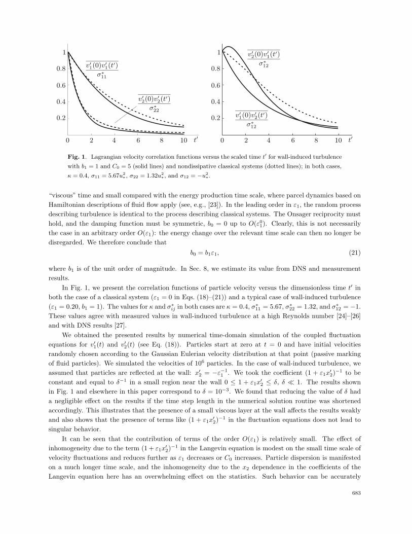
Fig. 1. Lagrangian velocity correlation functions versus the scaled time t′ for wall-induced turbulence

with b1 = 1 and C0 = 5 (solid lines) and nondissipative classical systems (dotted lines); in both cases,

κ = 0.4, σ11 = 5.67u2∗, σ22 = 1.32u2

∗, and σ12 = −u2∗.

“viscous” time and small compared with the energy production time scale, where parcel dynamics based onHamiltonian descriptions of fluid flow apply (see, e.g., [23]). In the leading order in ε1, the random processdescribing turbulence is identical to the process describing classical systems. The Onsager reciprocity musthold, and the damping function must be symmetric, b0 = 0 up to O(ε0

1). Clearly, this is not necessarilythe case in an arbitrary order O(ε1): the energy change over the relevant time scale can then no longer bedisregarded. We therefore conclude that

b0 = b1ε1, (21)

where b1 is of the unit order of magnitude. In Sec. 8, we estimate its value from DNS and measurementresults.

In Fig. 1, we present the correlation functions of particle velocity versus the dimensionless time t′ inboth the case of a classical system (ε1 = 0 in Eqs. (18)–(21)) and a typical case of wall-induced turbulence(ε1 = 0.20, b1 = 1). The values for κ and σ∗

ij in both cases are κ = 0.4, σ∗11 = 5.67, σ∗

22 = 1.32, and σ∗12 = −1.

These values agree with measured values in wall-induced turbulence at a high Reynolds number [24]–[26]and with DNS results [27].

We obtained the presented results by numerical time-domain simulation of the coupled fluctuationequations for v′1(t) and v′2(t) (see Eq. (18)). Particles start at zero at t = 0 and have initial velocitiesrandomly chosen according to the Gaussian Eulerian velocity distribution at that point (passive markingof fluid particles). We simulated the velocities of 106 particles. In the case of wall-induced turbulence, weassumed that particles are reflected at the wall: x′

2 = −ε−11 . We took the coefficient (1 + ε1x

′2)−1 to be

constant and equal to δ−1 in a small region near the wall 0 ≤ 1 + ε1x′2 ≤ δ, δ � 1. The results shown

in Fig. 1 and elsewhere in this paper correspond to δ = 10−3. We found that reducing the value of δ hada negligible effect on the results if the time step length in the numerical solution routine was shortenedaccordingly. This illustrates that the presence of a small viscous layer at the wall affects the results weaklyand also shows that the presence of terms like (1 + ε1x

′2)

−1 in the fluctuation equations does not lead tosingular behavior.

It can be seen that the contribution of terms of the order O(ε1) is relatively small. The effect ofinhomogeneity due to the term (1 + ε1x

′2)

−1 in the Langevin equation is modest on the small time scale ofvelocity fluctuations and reduces further as ε1 decreases or C0 increases. Particle dispersion is manifestedon a much longer time scale, and the inhomogeneity due to the x2 dependence in the coefficients of theLangevin equation here has an overwhelming effect on the statistics. Such behavior can be accurately

683

assessed by simulating the presented equations including integrating the time records of velocity to calcu-late displacements. In Sec. 9, we demonstrate similar behavior analytically using closed-form expressionsappropriate for the diffusion limit.

7. Generalization to the main section

Up to now, our attention was focused on the damping function for the inertial sublayer. Away fromthe wall and the inertial sublayer, in other words, in the main section x2/L = O(1), the statistical meansof fluctuating Eulerian velocities can no longer be assumed constant. A straightforward way to extend thepreviously obtained expressions for the damping function to the main section is to take the tensors λij andγij specified by Eqs. (11) and (12) to depend on x2, λij = λij(x2) and γij = γij(x2), via the dependenceof σij on x2. We note that the energy dissipation rate ε = ε(x2) is no longer approximated according toEq. (5), and well-mixing is based on Eq. (3) instead of (7). Langevin equation (14) can then be written inthe dimensional form

dv′idt

= −12(C0λij + b1γij)εv′j + φi +

√C0εwi(t), (22)

while particle positions can be described by (cf. Eqs. (2) and (4))

dxi

dt= u0

1(x2)δi1 + v′i. (23)

A term φi = φi(v, x2) describing the drift due to spatial changes of covariances is included in Eq. (22).Expressions for φi can be derived from the well-mixing condition, which corresponds to Eq. (3). Requiringthe well-mixing of first-order moments, i.e., multiplying Eq. (3) by u′

j, integrating over the entire u′ domain,and integrating by parts, we obtain

φi =dσi2

dx2. (24)

If we require Gaussianity of the fixed-point Eulerian velocities throughout the main section, then wecan describe the drift term according to Thomson as (see [16])

φi =dσi2

dx2+

12λjm

dσij

dx2(v′2v

′m − σ2m). (25)

But this formulation is not unique; other forms containing a quadratic relation for the velocities are possible,for example, the Borgas model [28]. The coefficients in all these formulations are proportional to theslope of the covariances, and all these formulations satisfy the well-mixing condition. Nevertheless, thenonuniqueness problem for φi is of the second order: the ultimate effect of the covariance inhomogeneity islimited because the terms containing C0ε in Eq. (22) are relatively large. For sufficiently large Re, we canidentify an inertial sublayer. Here, ε is very large (see Eq. (5)), and the contribution from the covarianceinhomogeneity via φi is very small. In this region, Eq. (22) is well described by Eq. (14) and becomesidentical to (14) if we pass to the limit of the inertial sublayer. In this case, the drift term vanishes. Inthe main section, ε decreases as the distance from the wall increases (see Eq. (5)), but the covarianceinhomogeneity effect remains small because the numerical value of C0 is rather large.

In summary, the contribution of the terms describing drift due to the covariance inhomogeneity is small.Compared with the leading terms in the damping function, the magnitude of the covariance inhomogeneityterms scales as C−1

0 x2L−1, where x2 is the distance from the wall and L is the external length, i.e., the pipe

radius, channel half-width, or turbulent boundary layer thickness along a wall or along the earth’s surface.While the contribution of the drift term φi is generally small, the contribution of the difference between

the two expressions for φi, denoted by ∆φi, is even smaller. At the marked point, the particle velocity

684

probability distribution equals that of the Eulerian velocity. The mean and standard deviation of ∆φi

are then equal to zero. It is only at long times that statistical means of ∆φi become nonzero. In Sec. 9,we present statistical descriptions of v′ valid in the long-time limit, i.e., the diffusion limit. They revealdifferences between the statistical values of the particle velocity and of the Eulerian velocity, which aresmall. The net effect is that the contribution to the particle dispersion from the terms relating to ∆φi isvery small. Numerical simulations reveal differences between the statistical values of particle displacementusing Eqs. (24) and (25) that are not larger than 2%. Dispersion predictions based on either (24) or (25)are equally good.

The linearly varying part of the damping function is the important term in Eq. (22). It consists of asymmetric part and an asymmetric part. The symmetric part constitutes the leading term in the expansionin C−1

0 . This symmetric part is unique. It is completely specified over the entire main section, i.e., no otherforms are possible, if we require the following for the formulation in the leading order in C0: Gaussianityof the fixed-point Eulerian velocities, well-mixing according to Eq. (3), and reciprocity analogous to theOnsager reciprocity. Asymmetry can occur in the damping only in terms of the order O(C−1

0 ) comparedwith the leading terms. Below, we establish the value of the parameter b1 = b1(x2) in these terms.

8. The value of the asymmetry parameter b1

We focus our attention on the (Lagrangian) correlation between the velocity of a passively markedfluid particle and its velocity at t = 0 at the position x2 = x20. Multiplying Eq. (22) by v′k(0), averaging,using the Markov property, expanding for small times t > 0, applying Gaussianity in the case of Eq. (25),and using Eqs. (11) and (12), we obtain

d(v′k(0)v′i(t)

)

dt= −1

2C0εδik − 1

2b1ε(δi1δk2 − δi2δk1) (26)

up to O(t). From this expression, we obtain the relation for the cross-correlation functions up to O(t),

d(v′1(0)v′2(t)

)

dt= −

d(v′2(0)v′1(t)

)

dt=

12b1ε. (27)

It can be seen that the value of b1 can be obtained directly from this relation. Estimates of the crosscorrelations in developed turbulent flow in a pipe of radius R0 at various radial positions and for Re =u∗R0/ν = 320 were recently obtained using three-dimensional particle tracking velocimetry [29]. We showresults from [29] in Fig. 2 and present values for b1 deduced from these results as a function of the distancefrom the wall in Fig. 3.

We estimated the slopes of cross correlations from the experimental data and obtained values forε by DNS of the same configuration. We also used the experimental results to estimate the value ofthe Kolmogorov constant from the Lagrangian velocity structure function [29]. We thus determined theKolmogorov constants appropriate for three directions and the difference between these values indicatesthe magnitude of the anisotropy. The degree of anisotropy determined by the differences between theKolmogorov constants in the streamwise and wall-normal directions C1 and C2 as a function of the walldistance is also shown in Fig. 3. It can be seen that the isotropy is maximum in the interior of the pipe.Here, the Reynolds number corresponding to the distance u∗x2/ν from the wall is largest, and a state ofisotropy of the small scales in accordance with Kolmogorov theory becomes visible. From the results at asmaller Reynolds number (u∗R0/ν = 180), we learned that the isotropy degree increases as Re increases [29]and the values of b1 overall decrease by approximately 15% over the entire radius. We can conclude that

685

Fig. 2. Cross correlations versus time (dots) and their slopes (straight lines) measured by three-

dimensional particle tracking in developed turbulent flow in a pipe of radius R0 for x20 = 0.5R0 and

Re = u∗R0/ν = 320 [29].

Fig. 3. The asymmetry coefficient b1 and anisotropy degree 2(C1 −C2)/(C1 + C2) inferred from the

measurements in [29].

the value of the asymmetry parameter b1 is less than unity in wall-induced turbulence at a high Reynoldsnumber.

Interestingly, cross-correlation functions do not seem to be affected by small “viscous” scales as t → 0,where τη =

√ν/ε is the Kolmogorov “viscous” time. While slopes of autocorrelations tend to zero as t → 0,

such behavior is not apparent in the cross correlations. This can be ascribed to the isotropy of viscous forces:the cross correlations of viscous forces are zero. Because of this behavior, we can rather precisely determinethe values of b1 from measured cross-correlations, even at not very high values of the Reynolds number.The experimentally determined slopes of the two relevant cross correlations also consistently showed themutual antisymmetry predicted by Eq. (27) and also seen in Fig. 2. The cross correlations derived fromthe DNSs, on the other hand, showed some deviations from the experimentally observed antisymmetricbehavior at certain radial positions. This may be due to an apparent anisotropic damping as a result ofapproximations in the numerical integration schemes. Alternatively, some anisotropic behavior of viscousforces present at a finite Reynolds number may have been filtered out during the measurements. In anycase, these differences are too small to affect the conclusions regarding the value of b1.

686

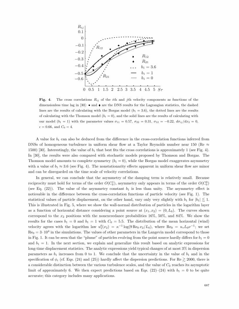
Fig. 4. The cross correlations Rij of the ith and jth velocity components as functions of the

dimensionless time lag in [30]: • and � are the DNS results for the Lagrangian statistics, the dashed

lines are the results of calculating with the Borgas model (b1 = 3.6), the dotted lines are the results

of calculating with the Thomson model (b1 = 0), and the solid lines are the results of calculating with

our model (b1 = 1) with the parameter values σ11 = 0.57, σ22 = 0.31, σ12 = −0.22, dσij/dx2 = 0,

ε = 0.66, and C0 = 4.

A value for b1 can also be deduced from the difference in the cross-correlation functions inferred fromDNSs of homogeneous turbulence in uniform shear flow at a Taylor Reynolds number near 150 (Re ≈1500) [30]. Interestingly, the value of b1 that best fits the cross correlations is approximately 1 (see Fig. 4).In [30], the results were also compared with stochastic models proposed by Thomson and Borgas. TheThomson model amounts to complete symmetry (b1 = 0), while the Borgas model exaggerates asymmetrywith a value of b1 ≈ 3.6 (see Fig. 4). The nonstationarity effects apparent in uniform shear flow are minorand can be disregarded on the time scale of velocity correlations.

In general, we can conclude that the asymmetry of the damping term is relatively small. Becausereciprocity must hold for terms of the order O(C1

0 ), asymmetry only appears in terms of the order O(C00 )

(see Eq. (22)). The value of the asymmetry constant b1 is less than unity. The asymmetry effect isnoticeable in the difference between the cross-correlation functions of particle velocity (see Fig. 1). Thestatistical values of particle displacement, on the other hand, vary only very slightly with b1 for |b1| � 1.This is illustrated in Fig. 5, where we show the wall-normal distribution of particles in the logarithm layeras a function of horizontal distance considering a point source at (x1, x2) = (0, L0). The curves showncorrespond to the x2 positions with the nonexceedance probabilities 16%, 50%, and 84%. We show theresults for the cases b1 = 0 and b1 = 1 with C0 = 5.5. The distribution of the mean horizontal (wind)velocity agrees with the logarithm law u0

1(x2) = κ−1 log(9 Re0 x2/L0), where Re0 = u∗L0ν−1; we set

Re0 = 3 ·104 in the simulations. The values of other parameters in the Langevin model correspond to thosein Fig. 1. It can be seen that the “plume” of particles evolving from the point source hardly differs for b1 = 0and b1 = 1. In the next section, we explain and generalize this result based on analytic expressions forlong-time displacement statistics. The analytic expressions yield typical changes of at most 3% in dispersionparameters as b1 increases from 0 to 1. We conclude that the uncertainty in the value of b1 and in thespecification of φi (cf. Eqs. (24) and (25)) hardly affect the dispersion predictions. For Re � 2000, there isa considerable distinction between the various turbulence scales, and the value of C0 reaches its asymptoticlimit of approximately 6. We then expect predictions based on Eqs. (22)–(24) with b1 = 0 to be quiteaccurate; this category includes many applications.

687

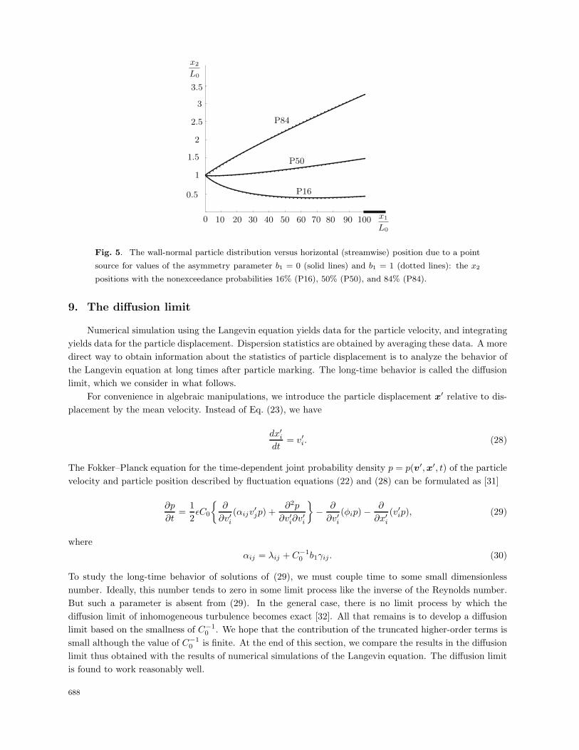
Fig. 5. The wall-normal particle distribution versus horizontal (streamwise) position due to a point

source for values of the asymmetry parameter b1 = 0 (solid lines) and b1 = 1 (dotted lines): the x2

positions with the nonexceedance probabilities 16% (P16), 50% (P50), and 84% (P84).

9. The diffusion limit

Numerical simulation using the Langevin equation yields data for the particle velocity, and integratingyields data for the particle displacement. Dispersion statistics are obtained by averaging these data. A moredirect way to obtain information about the statistics of particle displacement is to analyze the behavior ofthe Langevin equation at long times after particle marking. The long-time behavior is called the diffusionlimit, which we consider in what follows.

For convenience in algebraic manipulations, we introduce the particle displacement x′ relative to dis-placement by the mean velocity. Instead of Eq. (23), we have

dx′i

dt= v′i. (28)

The Fokker–Planck equation for the time-dependent joint probability density p = p(v′, x′, t) of the particlevelocity and particle position described by fluctuation equations (22) and (28) can be formulated as [31]

∂p

∂t=

12εC0

{∂

∂v′i(αijv

′jp) +

∂2p

∂v′i∂v′i

}− ∂

∂v′i(φip) − ∂

∂x′i

(v′ip), (29)

whereαij = λij + C−1

0 b1γij . (30)

To study the long-time behavior of solutions of (29), we must couple time to some small dimensionlessnumber. Ideally, this number tends to zero in some limit process like the inverse of the Reynolds number.But such a parameter is absent from (29). In the general case, there is no limit process by which thediffusion limit of inhomogeneous turbulence becomes exact [32]. All that remains is to develop a diffusionlimit based on the smallness of C−1

0 . We hope that the contribution of the truncated higher-order terms issmall although the value of C−1

0 is finite. At the end of this section, we compare the results in the diffusionlimit thus obtained with the results of numerical simulations of the Langevin equation. The diffusion limitis found to work reasonably well.

688

The adopted expansion procedure is similar to the methods van Kampen used to analyze the Kramersequation in [4]. Time is scaled as t = C0t

′, and Eq. (29) then becomes

∂

∂v′i(αijv

′jp) +

∂2p

∂v′i∂v′i= 2ε−1C−1

0

{∂

∂v′i(φip) +

∂

∂x′i

(v′ip)}

+ 2ε−1C−20

∂p

∂t′. (31)

Its solution can be written as an expansion in powers of C−10 :

p = p0 + C−10 p1 + C−2

0 p2.

Substituting this expression in (31) and equating like powers of C0 yields the equations

∂

∂v′i(αijv

′jp0) +

∂2p0

∂v′i∂v′i= 0, (32)

∂

∂v′i(αijv

′jp1) +

∂2p1

∂v′i∂v′i= 2ε−1

{∂

∂v′i(φip0) +

∂

∂x′i

(v′ip0)}

, (33)

∂

∂v′i(αijv

′jp2) +

∂2p2

∂v′i∂v′i= 2ε−1

{∂

∂v′i(φip1) +

∂

∂x′i

(v′ip1)}

+ 2ε−1 ∂p0

∂t′. (34)

The solution of (32) matching the distribution of the fixed-point Eulerian velocity at the instant of passivemarking is

p0(x, v, t) = G0(x, t)(2π)3/2λ1/2e−λijv′iv

′j/2, (35)

where λ is the determinant of λij ; we note that ∂(γijv′jp0)/∂v′i = 0. The function G0(x, t) describes the

distribution of the particle position or, equivalently, the distribution of the concentration of a passivelyadded admixture:

G0(x, t) =∫ +∞

−∞p0(x, v, t) dv. (36)

The equation for G0 = G0(x, t) can be derived from (33) and (34) as follows. A realistic solution for p2

is obtained from (34) if the integral of the right-hand side over the entire v domain is zero. Noting thatφip1 → 0 as |v| → 0, we have

− ∂

∂xi

∫ +∞

−∞v′ip1 dv =

∂G0

∂t. (37)

The integral can be evaluated by multiplying (33) by v′k and integrating by parts,

−αkj

∫ +∞

−∞v′jp1 dv = 2ε−1

{−

∫ +∞

−∞φkp0 dv +

∂

∂x′i

∫ +∞

−∞v′iv

′kp0 dv

}. (38)

Using Eq. (35) and multiplying by α−1ik , we obtain

∫ +∞

−∞v′ip1 dv = 2α−1

ik ε−1

{G0

dσk2

dx2− ∂

∂xj(σjkG0)

}= −2α−1

ik σjkε−1 ∂G0

∂x′j

. (39)

It was noted that ∫ +∞

−∞φip0 dv = G0

dσ2i

dx2

for both descriptions of φi, Eqs. (24) and (25), because the probability distribution of the particle velocityaccording to (35) equals that of the Eulerian fixed-point velocity, which results in the mean value of the

689

difference between the two expressions vanishing. We can therefore conclude that in the leading order of thediffusion limit, the dispersion results are unaffected by the nonuniqueness of φi! A difference between themean values of the two expressions for φi occurs only in higher orders. Considering higher-order solutionsfor p1 and p2, i.e., solutions of (33) and (34) not presented here, we found that the difference between thetwo mean values of φi scales as C−2

0 . Its ultimate contribution to the dispersion is very small and leads torelative deviations in statistical values of the dispersion of a few percent or less for values of C0 ≥ 5.

Substituting (39) in (37) yields the diffusion equation. Converting from the relative position x′ to x

and from the scaled time t′ to t, we obtain

∂G0

∂t+ u0

1

∂G0

∂x1=

∂

∂xi

(Dij

∂G0

∂xj

), (40)

where the diffusion coefficient Dij = Dij(x2) is defined as

Dij =2α−1

ik σjk

C0ε. (41)

The applicability of this result is not limited to the symmetric form of the linear damping function in theLangevin equation. The result also applies to asymmetric damping, whose effect appears via the tensor αij

given by (30). We can write

α−1ik σjk =

v−11 (σ2

12 + σ211) v−1

1

{σ12(σ11 + σ22) −

b1d

C0

}0

v−11

{σ12(σ11 + σ22) +

b1d

C0

}v−11 (σ2

12 + σ222) 0

0 0 σ233

, (42)

where v1 = 1 + b21/C2

0 and d = σ11σ22 − σ212. Substituting (42) in diffusion equation (40) and rearranging

terms gives∂G0

∂t+

{u0

1 −2

C20

∂

∂x2(v−1

1 b1dε−1)}

∂G0

∂x1=

∂

∂xi

(Ds

ij

∂G0

∂xj

), (43)

where Dsij is the symmetric diffusion tensor

Dsij =

2C0ε

v−11 (σ2

12 + σ211) v−1

1 σ12(σ11 + σ22) 0

v−11 σ12(σ11 + σ22) v−1

1 (σ212 + σ2

22) 0

0 0 σ233

.

The asymmetry effect now appears in a drift term in the mean flow direction and in a correction in thediffusivity tensor. The drift term is negligible: drift competes with convection by the mean flow, whichis very large in wall-induced turbulence at a large Reynolds number. But the correction in the diffusivitytensor is also very small because it involves the factor b2

1/C20 . For b1 = 1 and C0 = 5.5, this factor amounts

to 0.03. Deviations in the dispersion statistics due to possible variations of b1 between 0 and 1 thus amountto only 3%! This shows that the uncertainty due to a possible asymmetry in the damping function is anegligible factor in dispersion. At b1 = 0, the description of the diffusion tensor reduces to

Dij =2σikσjk

C0ε. (44)

Substituting this result in (40), we obtain a diffusion equation in which all uncertainty related to nonunique-ness has vanished. Because of the Onsager symmetry, which holds in the leading order in C0, the nonunique-ness uncertainty appears only in terms of the relative magnitude O(C−2

0 ). The contribution of these termscan be disregarded when allowing for errors in the dispersion parameters that are at most a few percent.

690

The remaining unanswered question is what the error is in the diffusion approximation because oftruncating the expansion in powers of C−1

0 leading to the diffusion approximation irrespective of the termsrelated to nonuniqueness. This question can be answered by deriving expressions for the higher-order termsin the expansion. But the expressions seem long and complicated. A more pragmatic approach is to comparethe results of the diffusion equation with the results of numerically simulating the Langevin equation. Indoing so, we focus attention on the inertial sublayer, where the Fokker–Planck equation reduces to Eq. (14).We must compare the statistics of the particle displacement in the wall-normal direction. These have aprimary importance because they also substantially determine the dispersion in the mean flow directionvia the x2 dependence of the mean flow u0

1(x2). The probability density of particle displacement in the x2

direction, denoted by G20 = G20(x2), is defined as

G20(x2) =∫ +∞

−∞

∫ +∞

−∞G0(x) dx1 dx3.

Integrating (43) over the entire x1 and x3 domain, taking the inertial sublayer limit, and setting b1 = 0, weobtain

∂G20

∂t= κ1u∗

∂

∂x2

(x2

∂G20

∂x2

), (45)

where

κ1 =2κ

C0

(1 +

σ222

u4∗

)(46)

and u∗ is the shear velocity.Expressions for the statistical moments xn

2 =∫ +∞−∞ xn

2 G20 dx2 are obtained by multiplying (45) by xn2 ,

integrating over the entire x2 domain and integrating the term in the right-hand side by parts. We thusobtain the first cumulant (cumulants are marked by a double overbar).

x∗2 = x∗

2 = 1 + κ1t∗, (47)

where x∗2 = x2/L0, L0 is the particle position at t = 0, and t∗ = u∗t/L0. Expressions for higher-order

moments can be derived similarly. Using the relations between moments and cumulants [4], we obtain

x∗22 = κ2

1t∗2 + 2κ1t

∗, x∗23 = 2κ3

1t∗3 + 6κ2

1t∗2, x∗

24 = 6κ4

1t∗4 + 24κ3

1t∗3. (48)

These results exhibit significant values for higher-order cumulants. The long-time limits of skewness

x∗23(

x∗22)−3/2

and kurtosis x∗24(

x∗22)−2

derived from these expressions are respectively 2 and 6, whichindicates a strong non-Gaussian behavior. This is a consequence of the inhomogeneity of wall-inducedturbulence reflected in the change of energy dissipation and diffusivity in the wall-normal direction.

In Fig. 6a, we show(

xn2

)1/n

for n = 1, 2, 3, 4 obtained by numerically simulating the Langevinequation appropriate for the logarithm layer divided by their respective values according to the diffusionlimit (cf. Eqs. (47) and (48)) as a function of the dimensionless time u∗t/L0. The parameter values used inthe comparison are listed in the figure caption. For times shortly after marking, the solutions of the diffusionequation differ considerably. The differences are inherent to the diffusion approximation, which is known toexhibit serious errors in the short-time limit. At long times, the ratios of the cumulants approach constantvalues, but they are less than unity by an amount that increases as n increases. This illustrates that thediffusion limit never becomes exact in inhomogeneous turbulent flow [32]. Nevertheless, the deviations arenot dramatic if we accept some inaccuracy in the tails of the probability distributions. The deviations canbe reduced by correcting the value of the diffusivity κ1 by multiplying it by 0.85 (see Fig. 6b).

691

a b

Fig. 6. The quotient of“

xn2

”1/n

calculated by numerically simulating the Langevin model for

the logarithm layer divided by its value (a) according to the diffusion limit and (b) according to a

“corrected” diffusion limit κ1 �→ 0.85κ1 : the results correspond to C0 = 5.5 and b1 = 0 and the other

parameter values are as in Fig. 1.

We also estimated the skewness and kurtosis from the simulations of the Langevin equation. Theirlong-time values were respectively found to be 1.6 and 3.4 for the given parameter values. These valuesshould be compared with the respective values 2 and 6 obtained using the diffusion approximation. Wenote that the long-time values of skewness and kurtosis in the case of the diffusion limit are insensitiveto the values of the diffusion constant. They cannot be adjusted by introducing some correction factor.The differences between skewness and kurtosis obtained from the Langevin equation and from the diffusionequation are pure manifestations of the truncation error in the diffusion approximation for a finite value ofC0. The error is decreased if we increase the value of the Kolmogorov constant.

10. The value of the Kolmogorov constant

The conventional approach for analyzing the spread of an admixture in a turbulent flow is to implementthe Boussinesq hypothesis leading to the semiempirical equation of turbulent dispersion [2]. The expressionsfor the diffusion coefficients used in this equation are based on the Reynolds analogy and are fitted tothe measurement results. As such, they can be considered calibrated coefficients reflecting observationalevidence. Comparing these coefficients with the theoretical diffusivity expressions obtained here yields someinteresting insights. It allows determining the value of the Kolmogorov constant C0.

The semiempirical equation for wall-normal dispersion in the logarithm layer of wall-induced turbulencecontains the diffusion coefficient stκu∗x2, where κu∗x2 follows from the Reynolds analogy with turbulentviscosity [2] and st is the turbulent Schmidt or Prandtl number, which serves to match model predictionsand measurement results. Over the past 50 years and more, many data have been collected for wall-normaladmixture dispersion and turbulent heat conduction. They lead to values of st between 0.9 and 1.1 (seevarious citations in [2]). Equating the empirical expression stκu∗x2 to κ1 defined by Eq. (46), setting st = 1,and setting σ22 = 1.32u2

∗ in agreement with experimental evidence, we find that C0 = 5.5. A more detailedanalysis of measurement data in the logarithm layer and using the Reynolds analogy (turbulent viscosity =turbulent diffusivity) leads to the same result. In general, we can conclude that the value of C0 is between 5and 6 based on the connection between the present theoretical diffusivity expressions and the experimentallydetermined diffusion coefficients. This compares well with values of C0 given in the literature [14]. Thevalues in the literature mostly originate from DNS results for homogeneous forms of turbulence. The

692

newness of the present specification of C0 is that it is based on results of measuring inhomogeneous wall-induced turbulence. This gives further confidence in the value of the universal Kolmogorov constant to beused in simulating the Langevin equation.

In [2], some indications are also given for the magnitudes and signs of the diffusion coefficients D11,D12, and D21 inferred from behavior in the atmospheric boundary layer. They are in line with the valuesobtained from Eqs. (41) and (42) if characteristic values are set for σij .

11. Summary and main conclusions

The starting point of our investigation was a description of the stochastic process of fluid particlemotion in wall-induced turbulence using a Langevin equation. Such an approach agrees with the asymptoticstructure of turbulence at a large Reynolds number. We took the white noise term in the equation inaccordance with the Lagrangian version of the inertial-sublayer limit of the ordinary Kolmogorov theoryof small scales. Some recent measurement results confirm the outcome of the Lagrangian theory of smallscales [6]. We did not consider refinements due to intermittency here because intermittency is known tohave little effect on the statistical means of particle displacement [9].

The main problem with the Langevin equation is the lack of a unique form for the damping term. Thisterm largely determines the Lagrangian statistics of velocities and displacements. We solved this problem inseveral steps. First, we took fixed-point Eulerian velocities to be Gaussian. Measurements largely supportthis assumption. They indicate typical skewness and kurtosis values of Eulerian velocities of 0.3 or less [17]–[19]. Second, we required well-mixing [16], in other words, the Eulerian interpretation of the Langevinequation should comply with the Gaussian distribution. This requirement leads to conditions on thedamping function but is insufficient for a complete specification. This problem is called the nonuniquenessproblem [7].

We solved the nonuniqueness problem by requiring a reciprocity analogous to the Onsager reciprocity.Viscous dissipation in the energy equation causes the principle of reciprocity to be applicable only overshort times. These times are proportional to the inverse of the Kolmogorov constant C0. Reciprocityis therefore only applicable for the leading term in an expansion of the damping function in powers ofC−1

0 . Nevertheless, applying the principle seems most rewarding. The uncertainty due to nonuniquenessis deferred to terms with higher powers of C−1

0 . It appears in two parts of the damping function: in theasymmetric part of the linear part of the damping term and in the drift term representing the effect ofcovariance inhomogeneity. We quantified the magnitude of the asymmetric damping term using recentmeasurement results for turbulent pipe flow based on particle tracking [29]. We estimated the uncertaintyeffects in the drift term by analyzing the long-time behavior of the Langevin equation. We thus foundthat nonuniqueness in both cases has an almost negligible effect on the particle displacement statistics.Their relative effect in both cases seems of the order O(C−2

0 ) in the stochastic description of particledisplacement, which is one order higher than in the Langevin equation for particle velocity! The effect canbe disregarded if errors of a few percent are allowed. This leads to a practically unique specification of theLangevin equation for describing the statistics of particle trajectories in wall-induced turbulence at a highReynolds number. More specifically, the dispersion of a passive admixture can be described by the systemof fluctuation equations

dv′idt

= −12C0ε(x2)σ−1

ij v′j +dσi2

dx2+

(C0ε(x2)

)1/2wi(t),

dxi

dt= u0

1(x2)δi1 + v′i,

where σij = σij(x2) = 〈u′iu

′j〉 is the covariance or Reynolds shear tensor.

693

In inhomogeneous turbulence, there is no limit process by which the diffusion approximation becomesexact [32]. To circumvent this difficulty, we introduced the inverse of the Kolmogorov constant as thesmall parameter in the long-time approximation of the Langevin model. The resulting diffusion equationinvolves truncation errors that are reasonably small for the means and standard deviations of displacementsbut become more serious for higher-order statistics. The diffusion equation appropriate for wall-inducedturbulence is given by

∂c

∂t+ u0

1(x2)∂c

∂x1=

∂

∂xi

(Dij(x2)

∂c

∂xj

),

where c is the passive admixture concentration and Dij = Dij(x2) is the turbulent diffusion coefficientdefined by Eq. (44). Relating the results in the diffusion limit to the large amount of experimentallyestablished diffusion coefficients over the past 50 years yields a value of the Kolmogorov constant C0

between 5 and 6.

REFERENCES

1. A. Kolmogoroff, C. R. Acad. Sci., 30, 301–305 (1941).

2. A. S. Monin and A. M. Yaglom, Statistical Fluid Mechanics: Mechanics of Turbulence [in Russian], Vol. 1,

Nauka, Moscow (1965); English transl., Dover, Mineola, N. Y. (2007).

3. G. I. Taylor, Proc. London Math. Soc. 2, 20, 196–211 (1922).

4. N. G. van Kampen, Stochastic Processes in Physics and Chemistry (Lect. Notes Math., Vol. 888), North-Holland,

Amsterdam (1981).

5. A. S. Monin and A. M. Yaglom, Statistical Fluid Mechanics: Mechanics of Turbulence [in Russian], Vol. 2,

Nauka, Moscow (1967); English transl., Dover, Mineola, N. Y. (2007).

6. G. A. Voth, A. La Porta, A. M. Crawford, J. Alexander, and E. Bodenschatz, J. Fluid Mech., 469, 121–160

(2002).

7. J. D. Wilson and B. L. Sawford, Boundary-Layer Meteorology , 78, 191–210 (1996).

8. A. H. Kolmogorov, “Precisions sur la structure locale de la turbulence dans un fluide visqueux aux nombres de

Reynolds eleves,” in: Mecanique de la turbulence (Colloq. Intern. CNRS, Marseille, Aug.-Sept. 1961), CNRS,

Paris (1962), pp. 447–458.

9. M. S. Borgas, Phil. Trans. Roy. Soc. London A, 342, 379–411 (1993).

10. M. S. Borgas and B. L. Sawford, Phys. Fluids, 6, 618–633 (1994).

11. U. Frisch, Turbulence: The Legacy of A. N. Kolmogorov , Cambridge Univ. Press, Cambridge (1995).

12. J. J. H. Brouwers, Phys. Fluids, 19, 101702 (2007).

13. M. S. Borgas and B. L. Sawford, J. Fluid Mech., 279, 69–99 (1994).

14. S. B. Pope, Turbulent Flows, Cambridge Univ. Press, Cambridge (2000).

15. F. Toschi and E. Bodenschatz, “Lagrangian properties of particles in turbulence,” in: Annual Review of Fluid

Mechanics, Vol. 41, Annual Review, Palo Alto, Calif. (2009), pp. 375–404.

16. D. J. Thomson, J. Fluid Mech., 180, 529–556 (1987).

17. J. Laufer, “The structure of turbulence in fully developed pipe flow,” Report No. 1174, http://naca.central.

cranfield.ac.uk/reports/1954/naca-report-1174.pdf, NACA (1954).

18. P. S. Klebanoff, “Characteristics of turbulence in a boundary layer with zero pressure gradient,” Report No. 1247,

http://naca.central.cranfield.ac.uk/reports/1955/naca-report-1247.pdf, NACA (1955).

19. J. F. Morrison, B. J. McKeon, W. Jiang, and A. J. Smits, J. Fluid Mech., 508, 99–131 (2004).

20. J. J. H. Brouwers, Phys. Fluids, 16, 2300–2308 (2004).

21. L. D. Landau and E. M. Lifshits, Statistical Physics: Part 1 [in Russian] (Vol. 5 of Course of Theoretical Physics),

Nauka, Moscow (1976); English transl. prev. ed., Pergamon, Oxford (1968).

22. L. E. Reichl, A Modern Course in Statistical Physics, Wiley, New York (1998).

23. O. Bokhove and M. Oliver, Proc. Roy. Soc. London A, 462, 2575–2592 (2006).

24. B. J. McKeon, J. Li, W. Jiang, J. F. Morrison, and A. J. Smits, J. Fluid Mech., 501, 135–147 (2004).

694

25. R. Zhao and A. J. Smits, J. Fluid Mech., 576, 457–473 (2007).

26. P. A. Monkewitz, K. A. Chauhan, and H. M. Nagib, Phys. Fluids, 19, 115101 (2007).

27. S. Hoyas and J. Jimenez, Phys. Fluids, 18, 011702 (2006).

28. B. L. Sawford and P. K. Yeung, Phys. Fluids, 12, 2033–2045 (2000).

29. R. J. E. Walpot, C. W. M. van der Geld, and J. G. M. Kuerten, Phys. Fluids, 19, 045102 (2007).

30. B. L. Sawford and P. K. Yeung, Phys. Fluids, 13, 2627–2634 (2001).

31. R. L. Stratonovich, Topics in the Theory of Random Noise, Vol. 1, General Theory of Random Processes,

Nonlinear Transformations of Signals and Noise, Gordon and Breach, New York (1967).

32. J. J. H. Brouwers, J. Engrg. Math., 44, 277–295 (2002).

695