laplace transform - unitn.itvisintin/laplace-2016.pdf · odes to algebraic equations. but the...
TRANSCRIPT
Laplace transform 1
Laplace transformNota: Una trattazione elementare ma piu ampia della transformazione di Laplace e offerta ad
esempio dal primo capitolo di
M. Marini: Metodi matematici per lo studio delle reti elettriche. C.E.D.A.M., Padova, 1999.
La seguente trattazione e basata in parte sul testo
G. Gilardi: Analisi tre. McGraw-Hill, Milano 1994.
This chapter includes the following sections:
1. Laplace transform of functions
2. Further Properties of the Laplace Transform
3. Laplace Transform of Distributions
4. Laplace Transform and Differential Equations
1 Laplace Transform of Functions
This transform is strictly related to that of Fourier, and like the latter it allows one to transformODEs to algebraic equations. But the Laplace transform is especially suited for the study of initialvalue problems, whereas the Fourier transform is appropriate for problems on the whole real line. Inapplications the theory of Laplace transform is also called symbolic or operational calculus.
From Fourier to Laplace transform. Let us first present some informal remarks. Let us denoteby u the Fourier transform of a transformable function u : R→ C:
u(ξ) :=1√2π
∫Ru(t)e−iξt dt for ξ ∈ R. (1.1)
The inversion formula is one of the main elements of interest of this transform:
u(t) :=1√2π
∫Ru(ξ)eiξt dξ for t ∈ R. (1.2)
This represents u as an (integral) average of the periodic functions wξ : R→ C : t 7→ eiξt parameterizedby ξ ∈ R and with weight u(ξ). Each of the functions wξ is called a harmonic with frequency ξ, 1 asw = wξ solves the equation of harmonic motion: 2
w′′(t) + ξ2w(t) = 0 for t ∈ R. (1.3)
Because of the classical method of variation of the constants, the solutions of this equation can beused for the study of the nonhomogeneous equation w′′(t) + ξ2w(t) = f(t) for t ∈ R, for a prescribedfunction f . (More specifically, one may look for a solution of the form w = zwξ, with wξ solution of(1.3) and z = z(t) to be determined. By replacing this expression in (1.3), we get the new equationz′′w + 2z′w′ = f , which is easily integrated.)
1 ξ represents the angular frequency, (also named pulsation), namely the ratio radians/time. Therefore ξ/(2π) is thefrequency, namely the ratio cycles/time.
2 Despite of (1.3), the functions wξ cannot be regarded as eigenfunctions of the second derivative in either L1 or L2,since they are not elements of either space.
2 Fourier Analysis, a.a. 2014-15 – A. Visintin
As |wξ(t)| ≤ 1 for any ξ, t ∈ R, the Fourier integral (1.2) converges for any u ∈ L1. Anyway wehave seen that one may also assume u ∈ L2, provided that the Fourier integral is understood in thesense of the principal value of Cauchy; and the domain of this transform can be further extended.
For any η ∈ R, let us also consider another equation of great interest:
w′(t) + ηw(t) = 0 for t ∈ R. (1.4)
The solutions of this equation are proportional to wη : R → R : t 7→ e−ηt; if η 6= 0, this functiondiverges exponentially as t→ +∞ or t→ −∞, depending on the sign of η. Analogously to (1.3), theclassical method of variation of the constants allows one to construct a solution for the nonhomogeneousequations w′(t) + ηw(t) = f(t). 3
In analogy with (1.1)), for the study of the equation w′(t) + ηw(t) = f(t) first we set
u(η) :=
∫Ru(t)e−ηt dt for η ∈ R. (1.5)
For any η > 0 (η < 0, respect.) this integral converges only if |u(t)| exponentially decays to 0 ast → −∞ (as t → +∞, respect.). Anyway in many cases of applicative interest the equation (1.4) isnot set on the whole R, but just on R+; in those cases it is convenient to restrict oneself to functionsthat vanish for any t < 0. 4
More generally, we can replace the real variable η by a complex variable s, since |e−st| = e−Re(s)t
for any t ∈ R (time remains real!). We can then consider the kernels R→ C : t 7→ e−st, parameterizedby s ∈ C. For imaginary s we retrieve periodic functions, whereas for real s these functions eithergrow or decay exponentially. 5 Let us then define the Laplace transform
u 7→ u(s) :=
∫Ru(t)e−st dt for s ∈ C, (1.6)
which includes (1.5) for s real and the Fourier transform for s imaginary (the conventional factor1/√
2π apart). Concerning the convergence of this integral, what we said for (1.5) holds here also, andwe shall confine ourselves to causal signals.
Setting s = x+ iy, we thus have
Ux(y) := u(x+ iy) =
∫Ru(t)e−xte−iyt dt for x, y ∈ R. (1.7)
The variable s is often referred to as a (complex) frequency, although just its imaginary part reallyrepresents a frequency, cf. (1.2). As Ux is the Fourier transform of the function t 7→
√2π u(t)e−xt,
(1.6) may be regarded as the Fourier transform of an array of inputs parameterized by x ∈ R.
The right side of (1.7) has a meaning whenever e−xtu(t) ∈ L1; if u is causal, the larger is x theless restrictive is this condition. This allows one to apply this formulation to the Laplace transformof a wide family of causal functions of L1
loc.6
3 Just as above, despite of (1.4), the functions wη cannot be regarded as eigenfunctions of the first derivative in eitherL1 or L2, since they are not elements of either space.
4 These are called causal signals in signal analysis. We shall occasionally refer to the terminology of this field ofengineering.
5 The functions u(η) cannot be regarded as eigenfunctions of the first derivative in S ′, since they do not belong tothat space.
6 There is thus little interest to extend this transform to L2.

Laplace transform 3
Functional set-up. The Laplace transform deals with functions of a single real variable, whichtypically represents time and is denoted by t. On the basis of the previous remarks, let us define theclass DL of the transformable functions, and for any u ∈ DL the abscissa of (absolute) convergenceλ(u), the convergence half-plane Cλ(u), and finally the Laplace transform L(u): 7
DL :={u ∈ L1
loc : u(t) = 0 q∀t < 0, ∃x ∈ R : e−xtu(t) ∈ L1t
}, (1.8)
λ(u) := inf{x ∈ R : e−xtu(t) ∈ L1
t
}(∈ [−∞,+∞[) ∀u ∈ DL, (1.9)
Cλ(u) := {s ∈ C : Re(s) > λ(u)} ∀u ∈ DL, (1.10)
[L(u)](s) :=
∫Re−stu(t) dt ∀s ∈ Cλ(u), ∀u ∈ DL. (1.11)
The transformed function L(u) is also called the Laplace integral. DL is the set of locally integrablecausal signals that have at most exponential growth. This is a linear space, and the Laplace transformis obviously linear: for any u, v ∈ DL ed ogni µ1, µ2 ∈ C,
λ(µ1u+ µ2v) = max{λ(u), λ(v)}, L(µ1u+ µ2v) = µ1L(u) + µ2L(v). (1.12)
The Lebesgue integral (1.11) converges for any s ∈ Cλ(u). For some functions this integral mayconverge also for some complex s with Re(s) = λ(u). But the Laplace transformed function L(u) isdefined just in Cλ(u), since some properties might fail if Re(s) ≤ λ(u).
Although we called Cλ(u) the convergence half-plane, w We do not exclude Cλ(u) = C (which westill call the convergence half-plane). Indeed λ(u) = −∞ if the transformable functions decays morethan exponentially; in particular this occurs for any compactly supported function of DL. On theother hand, we exclude Cλ(u) = ∅, i.e. λ(u) = +∞.
In the definition of the elements of DL we shall often encounter the Heaviside function H (alsocalled unit step):
H(t) := 0 ∀t ≤ 0, H(t) := 1 ∀t > 0.
The occurrence of the factor H(t) will guarantee causality. For instance, it is easily checked that
H(t) ∈ DL, λ(H) = 0,
tαH(t) ∈ DL, λ(tαH(t)) = 0 ⇔ Re(α) > −1;(1.13)
e−t2H(t) ∈ DL, λ(e−t
2H(t)) = −∞; et
2H(t), t−1H(t) 6∈ DL. (1.14)
The next result relates the Fourier and Laplace transforms.
Theorem 1.1. For any u ∈ DL,
[L(u)](x+ iy) =√
2π[F(e−xtu(t))
](y) ∀y ∈ R,∀x > λ(u). (1.15)
7 We write L1t in order to make clear that t is the integration variable.
Here we speak of abscissa of absolute convergence since the Lebesgue integral is absolutely convergent. Some authorsdefine the Laplace transform as an improper integral, rather than as a Lebesgue integral. Accordingly, they do notprescribe absolute convergence; this has some analogy with what we shall do ahead extending the Laplace transform todistributions. This has some consequences on some properties of the transform.
What we introduced is called the unilateral Laplace transform, as the domain of convergence is a half-plane. Inliterature a bilateral Laplace transform is also defined: in this case u need not be causal. The domain of convergence isthen a strip of the form {s ∈ C : λ1(u) < Re(s) < λ2(u)}, with −∞ ≤ λ1(u) < λ2(u) ≤ +∞. This bilateral transform ismuch less used than the unilateral one.
4 Fourier Analysis, a.a. 2014-15 – A. Visintin
Vice versa, u ∈ DL and λ(u) ≤ 0 for any causal u ∈ L1. If u ∈ L1 and λ(u) < 0 then 8
[F(u)](y) =1√2π
[L(u)](iy) ∀y ∈ R. (1.16)
By the foregoing result, several properties of the Fourier transform are easily extended to theLaplace transform. This also applies to the next statement.
Proposition 1.2. For any u ∈ DL,
v(t) = u(t− t0) ⇒ λ(v) = λ(u), v(s) = e−t0s u(s) ∀t0 > 0, (1.17)
v(t) = es0tu(t) ⇒ λ(v) = λ(u) + Re(s0), v(s) = u(s− s0) ∀s0 ∈ C, (1.18)
v(t) = u(ωt) ⇒ λ(v) = ωλ(u), v(s) = 1ω u(sω
)∀ω > 0. (1.19)
The assertions about convergence abscissas are easily checked: the delay does not modify thebehaviour of the function for t→ +∞; the exponential factor es0t instead entails a translation of theconvergence abscissa.
Examples. For any u ∈ DL,
u(t) = H(t) ⇒ λ(u) = 0, u(s) =1
s, (1.20)
u(t) = eγtH(t) (γ ∈ C) ⇒ λ(u) = Re(γ), u(s) =1
s− γ, (1.21)
u(t) = cos(ωt)H(t) (ω ∈ R) ⇒ λ(u) = 0, u(s) =s
s2 + ω2, (1.22)
u(t) = sin(ωt)H(t) (ω ∈ R) ⇒ λ(u) = 0, u(s) =w
s2 + ω2, (1.23)
u(t) = cosh(ωt)H(t) (ω ∈ R) ⇒ λ(u) = |ω|, u(s) =s
s2 − ω2, (1.24)
u(t) = sinh(ωt)H(t) (ω ∈ R) ⇒ λ(u) = |ω|, u(s) =w
s2 − ω2, (1.25)
u(t) = tkH(t) (k ∈ N) ⇒ λ(u) = 0, u(s) =k!
sk+1. (1.26)
The reader is asked to check these properties.The final formula is generalized by
u(t) = taH(t) (a > −1) ⇒ λ(u) = 0, u(s) =Γ(a+ 1)
sa+1, (1.27)
since, by definition of the classical Euler function Γ,
u(s) =
∫ +∞
0e−stta dt =
1
sa+1
∫ +∞
0e−yya dy =:
Γ(a+ 1)
sa+1∀s ∈ Cλ(u) = C0.)
Incidentally, notice that 1/s is definite for any complex s 6= 0, but H(s) = 1/s only if Re(s) >λ(H) = 0.
8 For λ(u) = 0 there is a formal inconvenience: if y ∈ R, [F(u)](y) obviously exists as u ∈ L1; but, as we saw, in thiscase it is not legitimate to write [L(u)](iy).

Laplace transform 5
The Laplace transform operates on periodic functions in a different way from the Fourier transform,as it is shown by the next result. Notice that, because of causality, here u is assumed to be therestriction of a periodic function only for positive time.
Theorem 1.3. (Periodic Functions) For any T > 0, let u ∈ DL, u 6≡ 0 be such that u(t+ T ) = u(t)for any t > 0. Then λ(u) = 0 and, setting
w(t) := u(t) ∀t ∈ [0, T ], w(t) := 0 ∀t ∈ R \ [0, T ], (1.28)
we have
u(s) =1
1− e−sTw(s) ∀s ∈ C0. (1.29)
Notice that 1 − e−sT 6= 0 for any s ∈ C0, and that the hypotheses entail that u ∈ L1(0, T ), butnot u ∈ L∞(0, T ).
Proof. For any x > 0, changing the integration variable, using the periodicity and setting C :=∫ T0 |w(τ)| dτ ( 6= 0 as u 6≡ 0), we have∫
Re−xt|u(t)| dt =
∞∑n=0
∫ (n+1)T
nTe−xt|u(t)| dt =
∞∑n=0
e−nTx∫ T
0e−xτ |w(τ)| dτ
(as e−xτ ≤ 1) ≤∞∑n=0
e−nTx∫ T
0|w(τ)| dτ = C
∞∑n=0
e−nTx < +∞.
(1.30)
On the other hand, for any x < 0,∫Re−xt|u(t)| dt =
∞∑n=0
∫ (n+1)T
nTe−xt|u(t)| dt =
∞∑n=0
e−nTx∫ T
0e−xτ |w(τ)| dτ
(as e−xτ ≥ 1) ≥∞∑n=0
e−nTx∫ T
0|w(t)| dt = C
∞∑n=0
e−nTx = +∞.
(1.31)
It follows that λ(u) = 0. 9 Setting uT (t) := u(t− T ) for any t ∈ R and noticing that w = u− uT , wehave
w(s) = u(s)− uT (s) = u(s)− e−sT u(s)(1.17)
= (1− e−sT )u(s) ∀s ∈ Cλ(u),
that is (1.29). tu
Theorem 1.4. (Convolution Theorem) For any u, v ∈ DL, u ∗ v ∈ DL and
λ(u ∗ v) ≤ max{λ(u), λ(v)}, L(u ∗ v) = L(u) L(v). (1.32)
More generally, for any integer N ≥ 2 and for any u1, ..., uN ∈ DL, we have u1 ∗ ... ∗ uN ∈ DL and
λ(u1 ∗ ... ∗ uN ) ≤ max{λ(ui) : i = 1, ..., N}, L(u1 ∗ ... ∗ uN ) =N∏i=1
L(ui). (1.33)
9 More synthetically, one may notice that, as u is periodic and integrable in any interval of the form ]nT, (n+ 1)T [,e−xtu(t) ∈ L1 for all x > 0 and for no x < 0. Therefore λ(u) = 0.
6 Fourier Analysis, a.a. 2014-15 – A. Visintin
The inequality (1.32) may be strict: e.g. consider u ≡ 0 and any v ∈ DL.The proof of (1.32) mimics that of the Fourier transform of the convolution, and is left to the
reader. (1.33) follows from (1.32) by recurrence.
Corollary 1.5. For any u ∈ DL, U(t) =∫ t
0 u(τ) dτ ∈ DL and
λ(U) ≤ max{λ(u), 0}, [L(U)](s) = [L(u)](s)/s if Re(s) > max {λ(u), 0}. (1.34)
Proof. As u is causal,∫ t
0 u(τ) dτ =∫ t−∞ u(τ) dτ = (u ∗H)(t) for any t > 0. It then suffices to apply
the convolution theorem. tu
Theorem 1.6. (Holomorphy) For any u ∈ DL,
the function u is holomorphic in Cλ(u), (1.35)
∀λ > λ(u), the function u is bounded in the half-plane {s ∈ C : Re(s) ≥ λ}, (1.36)
supIm(s)∈R
u(s)→ 0 for Re(s)→ +∞. (1.37)
Proof. The proof of holomorphism is analogous to that we saw for the Fourier transform, and is leftto the reader. (One may actually differentiate w.r.t. s under the integral.) (1.36) holds true as
|u(s)| ≤∫Re−tλ|u(t)| dt ∀λ ∈ ]λ(u),Re(s)[. (1.38)
By passing to the limit as Re(s) → +∞ in this inequality via the dominated convergence theorem,(1.37) follows. tu
Incidentally, notice that the transformed function u need not be bounded at the interior of thewhole half-plane Cλ(u). The transform H(s) = 1/s is a counterexample.
Remarks. (i) If the Laplace integral absolutely converges for some s ∈ C, then the same occurs fors+iy for any y ∈ R. Therefore the set of absolute convergence is either of the form {s ∈ C : Re(s) > a}or {s ∈ C : Re(s) ≥ a} for some a ∈ ]−∞,+∞[ (or it is the whole C).
(ii) In some cases u may be extended to a holomorphic function defined on a larger domain thanCλ(u). For instance, the transform H(s) (= 1/s) of the Heaviside function H is only defined forRe(s) > λ(H) = 0, although the function s 7→ 1/s is holomorphic in C \ {0}.
(iii) The theorem of holomorphism is one of the main differences between the properties of theLaplace and Fourier transforms, as in general Fourier transformed functions need not be holomorphic.
For instance, the function w : R→ C : ξ 7→ (1 + ξ2)−2 is an element of L2, hence it is the Fouriertransform of some function u ∈ L2. However, w has no holomorphic continuation to the whole C, as(1 + s2)−2 is not defined for s = ±i.
(iv) In several cases the theorem of holomorphism allows one to perform a computation for real s,and then to extend the result to the convergence half-plane. tu
2 Further Properties of the Laplace Transform
For the differentiation of the original function and of its Laplace transform, we have analogous rulesto those we saw for the Fourier transform. In one of these formulas the initial value of the function

Laplace transform 7
u occurs. 10 We remind the reader that for any function v = v(t), by Dv we denote the derivativein the sense of distributions (which exists for any v), and by v′ the derivative almost everywhere (ifexisting).
Proposition 2.1. (Laplace transform and a.e. differentiation) (i) For any u ∈ DL,
tu(t) ∈ DL, λ(tu(t)) = λ(u),
[L(u)]′(s) = −[L(tu(t))](s) ∀s ∈ Cλ(u).(2.1)
More generally, for any n ∈ N,
tnu(t) ∈ DL, λ(tnu(t)) = λ(u),
[L(u)](n)(s) = (−1)n[L(tnu(t))](s) ∀s ∈ Cλ(u).(2.2)
(ii) For any u ∈ DL that is absolutely continuous in ]0,+∞[, if u′ ∈ DL and if there exists
u(0+) := limt→0+
u(t) ∈ C,
then[L(u′)](s) = s[L(u)](s)− u(0+) ∀s ∈ Cλ(u) ∩Cλ(u′). (2.3)
Proof. As we saw, multiplication by t does not modify the convergence abscissa of u. The proof ofthe formula L(u)′ = −L(tu(t)) (the derivative of a holomorphic function) is straightforward.
Let us next check (2.3). As e−stu(t) ∈ L1t whenever Re(s) > λ(u), there exists a diverging sequence
{tn} such that e−stnu(tn)→ 0 as n→ +∞. By partial integration we then get
[L(u′)](s) =
∫ +∞
0e−stu′(t) dt = lim
n→∞
∫ tn
0e−stu′(t) dt
= limn→∞
{∫ tn
0se−stu(t) dt+ e−stnu(tn)
}− u(0+)
= s
∫ +∞
0e−stu(t) dt− u(0+) ∀s ∈ Cλ(u) ∩Cλ(u′). tu
(2.4)
Remarks. (i) If u ∈ DL is absolutely continuous in ]0,+∞[, let us denote by u′ the causal functionthat coincides with the ordinary derivative in ]0,+∞[. This does not entail u′ ∈ DL. For instanceu1(t) = t−1/2H(t) and u2(t) = [sin exp(t2)]H(t) are both elements of DL, but u′i 6∈ DL for i = 1, 2.
(ii) In part (ii) of the latter theorem, the hypothesis u′ ∈ DL cannot be dropped. Indeed the a.e.differentiability of u alone does not entail (2.3), as u might have a jump at some t > 0. As we know,these discontinuities entail the occurrence of Dirac masses in Du.
The formula (2.3) is easily extended to higher-order derivatives.
Proposition 2.2. Let u ∈ DL be such that u, u′, ..., u(m−1) are absolutely continuous in ]0,+∞[ foran integer m > 1. If u′, ..., u(m) ∈ DL and if the limits u(0+), ..., u(m−1)(0+) exist in C, then
[L(u(m))](s) = sm[L(u)](s)−m−1∑n=0
sm−n−1u(n)(0+) ∀s ∈ Cλ(u) ∩ ... ∩Cλ(u(m)). (2.5)
10 When dealing with the Laplace transform of distributions we shall illustrate this issue.
8 Fourier Analysis, a.a. 2014-15 – A. Visintin
Proof. For instance, for m = 2 by applying Proposition 2.1 first to u′ and then to u, we get
[L(u′′)](s) = s[L(u′)](s)− u′(0+) = s2[L(u)](s)− su(0+)− u′(0+)
for any s ∈ Cλ(u) ∩Cλ(u′) ∩Cλ(u′′). The equality (2.5) is easily proved by recurrence. tu
Proposition 2.3. (Laplace transform and integration) If u, u(t)/t ∈ DL then λ(u(t)/t) = λ(u) and11
[L(u(t)/t)](s) = limR3σ→+∞
∫ σ
s[L(u)](r) dr ∀s ∈ Cλ(u). (2.6)
This limit coincides with the generalized integral of L(u) between s and +∞ (here +∞ is thelimit of (x, 0) as x → +∞...); this integral does not depend on the integration path, because L(u) isholomorphic. Anyway it need not converge absolutely, hence it may not be representable as a Lebesgueintegral. 12
Proof. As∫ t
0 u(τ)dτ = (u∗H)(t), the convolution theorem yields[L(∫ t
0u(τ)dτ
)](s) = u(s)H(s) =
u(s)
sif Re(s) > max {λ(u), 0}.
On the other hand, if u, u(t)/t ∈ DL then by applying the differentiation theorem to v(t) := u(t)/twe have
λ(u(t)/t) = λ(u), L(v)′ = −L(tv(t)) = −L(u),
whence by integration
v(s) = v(σ) +
∫ σ
s[L(u)](r) dr ∀s ∈ Cλ(u), ∀σ > λ(u).
Passing to the limit as σ → +∞ and recalling (1.37), we get (2.6). tu
The next theorem is an example of the so-called Tauberian theorems. These results provide infor-mation on the original function u on the basis of the transformed function u, without inverting theLaplace transformation.
Theorem 2.4. *(of final and initial values) For any u ∈ DL, 13
∃u(+∞) ∈ C ⇒ λ(u) ≤ 0, su(s)→ u(+∞) as s→ 0, (2.7)
∃u(0+) ∈ C ⇒ supIm(s)∈R |su(s)− u(0+)| → 0 as Re(s)→ +∞. (2.8)
If λ(u) = 0 then in (2.7) it is understood that s → 0 from the half-plane of complex numberswith positive real part. The convergence in (2.8) is tantamount to the following: as Re(s) → +∞,su(s)→ u(0+) uniformly w.r.t. Im(s).
* Proof. In order to simplify the argument, for both statements we shall assume that
u is absolutely continuous in ]0,+∞[, u′ ∈ DL, ∃u(+∞), ∃u(0+). (2.9)
11 Here we mean that σ is real; anyway, because of the holomorphism of L(u), this limit may also be taken as σ variesalong a complex path in Cλ(u).
12 In formula (2.6) we do not write∫ +∞s
[L(u)](τ) dτ , as we reserve the integral notation to the Lebesgue integral.13 We set u(+∞) := limt→+∞ u(t) whenever this limit exists (in C).
Laplace transform 9
As the function u is continuous and converges as t → 0 and t → +∞, u is bounded and thusλ(u) ≤ 0. Because of the dominated convergence theorem, we have∫ +∞
0u′(t) dt = lim
s→0
∫ +∞
0e−stu′(t) dt = lim
s→0[L(u′)](s)
(2.3)= lim
s→0su(s)− u(0+). (2.10)
On the other hand∫ +∞
0u′(τ) dτ = lim
t→+∞
∫ t
0u′(τ) dτ = lim
t→+∞u(t)− u(0+) = u(+∞)− u(0+), (2.11)
and by comparing these two identities we get (2.7).Similarly, we have
limRe(s)→+∞
su(s)− u(0+)(2.3)= lim
Re(s)→+∞[L(u′)](s)
(1.37)= 0, (2.12)
and this limit is uniform respect to Im(s). (2.8) is thus proved. tu
Remarks. (i) The final-value theorem cannot be inverted: the existence of lims→0 su(s) in C doesnot entail that of u(+∞). For instance u(t) = (sin t)H(t) does not converge as t → +∞, althoughsu(s) = s/(s2 + 1)→ 0 as s→ 0.
(ii) The initial-value theorem also cannot be inverted: the existence of limRe(s)→+∞ su(s) in C(uniformly w.r.t. Im(s)) does not entail that of u(0+). We omit the counterexample, which is lesssimple than the previous one.
Inversion of the Laplace transform. The following theorem provides an explicit formula for theantitransform. This is derived by reducing the Laplace transform to the Fourier transform, see (1.16).
Let us first say that a function u ∈ DL is of exponential order if
∃α ∈ R,∃M > 0 : |u(t)| ≤Meαt for a.e. t > 0. (2.13)
This class includes most of the functions that occur in applications. Not all elements of DL areof exponential order, but any nondecreasing u ∈ DL has this property. [Ex] For any u ∈ DL ofexponential order, λ(u) is the infimum of the α ∈ R that fulfill (2.13).
Theorem 2.5. (Riemann-Fourier) If u ∈ DL is of exponential order, then, denoting by u its Laplacetransform,
u(t) =1
2πiP.V.
∫x+iR
estu(s) ds
(=
1
2πlim
R→+∞
∫ R
−Re(x+iy)tu(x+ iy) dy
)q∀t ∈ R,∀x > λ(u).
(2.14)
Proof. Let us select any x > λ(u) and set
ϕx(y) := u(x+ iy) =
∫Re−(x+iy)tu(t) dt ∀y ∈ R,
that is, ϕx(y) =√
2π[F(e−xtu(t))](y). By (2.13), λ(u) ≤ α; as x > λ(u), then
∃α ∈ ]λ(u), x[: Mα := ess supt>0
{e−αt|u(t)|} < +∞; [Ex]

10 Fourier Analysis, a.a. 2014-15 – A. Visintin
hence|e−(x+iy)tu(t)| = |e−xtu(t)| = |e−αtu(t)|e(α−x)t ≤Mαe
(α−x)t ∈ L2.
The Fourier transform F(e−xtu(t)) may thus be understood not only in the sense of L1 (i.e., as aLebesgue integral) but also in the sense of L2, thus as a principal value. The theorem of inversion ofthe Fourier transform in L2 then yields
e−xtu(t) =1√2π
[F−1(ϕx)
](t) =
1
2πP.V.
∫Reityϕx(y)dy q∀t ∈ R,∀x > λ(u), (2.15)
that is, (2.14). tu
An exercise in complex calculus. Next we directly check that the principal value occurring in(2.14) does not depend on x > λ(u). Here we assume that
∃ C, a > 0 : ∀s ∈ Cλ(u) |u(s)| ≤ C|s|−a, (2.16)
although, because of the previous argument, this additional hypothesis is not really needed.For any x1, x2 with λ(u) < x1 < x2, because of Proposition 1.6 the function s 7→ estu(s) is ho-
lomorphic in the strip of the complex plane that is comprised between the straight lines x1 + iRand x2 + iR. For any R > 0 let us denote by BR the boundary of the rectangle of verticesx1 − iR, x1 + iR, x2 + iR, x2 − iR. By the classical Cauchy integral theorem,∫
BR
estu(s)ds = 0 ∀R > 0. (2.17)
Because of (2.16) the modulus of the integral along the horizontal segment y = R is dominated by∫ x2
x1
ext|u(x+ iR)| dx ≤ Cex2t|x1 + iR|−a(x2 − x1),
which vanishes as R → +∞. The same holds for the modulus of the integral along the horizontalsegment y = −R. (2.17) then yields∫ x1+iR
x1−iRestu(s)ds−
∫ x2+iR
x2−iRestu(s)ds→ 0 for R→ +∞.
As both these integrals converge in the sense of the principal value as R→ +∞, hence
1
2πiP.V.
∫x1+iR
estu(s) ds =1
2πiP.V.
∫x2+iR
estu(s) ds.
Remark. The inversion formula requires the evaluation of integrals along paths in the complex field(so-called contourn integrals), and this may be cumbersome. In several cases it is more convenient toantitransform a function by expanding it in simple fractions, and then use transform tables backward,as we shall see in the next section.
This result also entails that the Laplace transform is injective on the whole DL.
Antitransformability. The problem of characterizing the class L(DL) of transformed functions isnontrivial. Here we just provide a sufficient condition for existence of the inverse transform.

Laplace transform 11
Theorem 2.6. (Antitransformability-I) The restriction of a function U of complex variable to asuitable half-plane is the Laplace transform of some function T ∈ DL if 14
∃λ ∈ R : U is holomorphic for Re(s) > λ, (2.18)
∃α > 1 : supy∈R |x+ iy|αU(x+ iy)→ 0 as x→ +∞. (2.19)
This implication cannot be inverted. For instance, the condition (2.19) fails for the functionU(s) = 1/s, which however is the transform of the Heaviside function for Re(s) > 0. 15 This exampleand the theorem above yield the next result, which is often applied because of the ubiquity of theHeaviside function.
Corollary 2.7. Let U be a complex function of complex variable which fulfills the hypotheses ofTheorem 2.6, then the functions V of the form
V (s) = U(s) +a
s∀s ∈ Cλ (for some a ∈ C and λ > 0), (2.20)
are also antitransformable, and L−1(V ) = L−1(U) + aH.
Therefore any function V that can be represented as a sum of the form (2.20) is antitransformable.
3 Laplace Transform of Distributions
We saw that the Laplace transform extends the Fourier transform in L1. As the latter transform canbe extended to the space S ′ of tempered distributions, one may wonder whether the Laplace transformcan also be extended to some space of distributions. We shall answer in the affirmative, under suitablerestrictions.
Let us define the class DL of transformable distributions with convergence abscissa λ: 16
DL :={T ∈ D′ : supp(T ) ⊂ R+,∃x ∈ R : e−xtT (t) ∈ S ′t
}, (3.1)
λ(T ) := inf{x ∈ R : e−xtT (t) ∈ S ′t
}(∈ [−∞,+∞[) ∀T ∈ DL, (3.2)
Cλ(T ) := {s ∈ C : Re(s) > λ(T )} ∀T ∈ DL. (3.3)
We are tempted to write a formula like (1.11), simply by replacing the integral with a suitableduality pairing 〈·, ·〉. May we set
[L(T )](s) = 〈T (t), e−st〉 ∀s ∈ Cλ(T ),∀T ∈ DL ? (3.4)
Here we cannot use the duality pairing between D′ and D as the support of e−st is not compact (andthe same holds for e−stH(s)). Even if T ∈ S ′, we cannot use the pairing between S ′ and S, since e−st
14 (2.19) is tantamount to ∃α > 1 : ∀ε > 0,∃L > 0 such that if Re(s) > L then |s|α|U(s)| ≤ ε.This means that, for a suitable α > 1, |s|αU(s)→ 0 as Re(s)→ +∞, uniformly w.r.t. Im(s).15 Incidentally, notice that, although the function U is not integrable on x + iR for x > 0, one can apply the
Riemann-Fourier formula (2.14), as there the integral is meant in the sense of the principal value.16 As we know, the condition supp(T ) ⊂ R+ means that 〈T, v〉 = 0 for any v ∈ D such that supp(v) ⊂ ]−∞, 0[. We
use the notation S ′t to indicate that t is the independent variable; here x is just a parameter.At variance of what we did for the Laplace transform of functions, which was defined by a Lebesgue integral, here we
do not speak of abscissa of absolute convergence, as this is meaningless for duality pairings.
12 Fourier Analysis, a.a. 2014-15 – A. Visintin
does not decay exponentially as t→ +∞ whenever Re(s) ≤ 0. On the other hand, we do not expectto encounter any substantial difficulty for t→ −∞, since the support of T is confined to R+.
We then use the following construction. First, we fix any function ζ ∈ C∞ such that
ζ = 0 in ]−∞, a[, for some a < 0, ζ = 1 in R+.
For any T ∈ DL and any s ∈ Cλ(T ), we then select any x ∈ ]λ(T ),Re(s)[. Notice that e−xtT (t) ∈ S ′
because of (3.2), and e(x−s)tζ(t) ∈ S as Re(x− s) < 0. We then set
[L(T )](s) := S′〈e−xtT (t), e(x−s)tζ(t)〉S ∀s ∈ Cλ(T ), ∀T ∈ DL. (3.5)
It is not difficult to check that this value does not depend on the choice of x ∈ ]λ(T ),Re(s)[ and ofthe function ζ. [Ex] This definition is thus formally equivalent to (3.4), which may be regarded justas a short-writing of the rigorous formula (3.5).
Here is an important example:
[L(δa)](s) = e−as ∀s ∈ C,∀a ≥ 0. (3.6)
Notice that δa := δ0(· − a) is causal iff a ≥ 0.As L1 ⊂ S ′, the transform L of distributions extends that of functions (that we denoted by L):
DL ⊂ DL, (3.7)
λ(u) ≤ λ(u) i.e. Cλ(u) ⊂ Cλ(u) ∀u ∈ DL, (3.8)
L(u)|Cλ(u) = L(u) ∀u ∈ DL. (3.9)
Moreover, the use of duality pairing instead of the (Lebesgue) integral overcomes the restriction ofabsolute convergence.
We shall also see that:(i) there exists u ∈ L1
loc such that u ∈ DL \DL — thus L 6= L∣∣DL∩L1
loc;
(ii) there exists u ∈ DL such that λ(u) < λ(u) — thus L 6= L∣∣DL
, despite of (3.9).
Alike what we saw for functions, the Laplace transform of distributions is holomorphic.
Proposition 3.1. For any T ∈ DL, the function L(T ) is holomorphic in Cλ(T ). []
Anyway (1.36) and (1.37) do not take over to distributions; e.g., L(Dδ0) = s for any s ∈ C.Theorems 1.1, 1.2, 1.3, 1.4 also hold in DL. The same applies to the inversion formula, under
hypotheses that here we do not display.
Next we extend the transform of the derivative, under weaker hypotheses and by a simpler for-mula than for functions. We remind the reader that by D we denote the derivative in the sense ofdistributions.
Theorem 3.2. (Laplace transform of the distributive derivative) For any T ∈ DL,
DT ∈ DL, λ(DT ) ≤ λ(T ), [L(DT )](s) = s[L(T )](s) ∀s ∈ Cλ(T ). (3.10)
More generally, for any k ∈ N,
DkT ∈ DL, λ(DkT ) ≤ λ(T ), [L(DkT )](s) = sk[L(T )](s) ∀s ∈ Cλ(T ). (3.11)
Laplace transform 13
Proof. Because of Theorem 1.1, (3.10) stems from the analogous formula for the Fourier transformof distributions. (3.11) then follows by induction. tu
For instance,
[L(Dkδa)](s) = ske−as ∀s ∈ C, ∀a ≥ 0,∀k ∈ N. (3.12)
Let u ∈ DL and assume that u is absolutely continuous in ]0,+∞[, that u′ ∈ DL and that thereexists u(0+) := limt→0+ u(t) ∈ C. By part (ii) of Theorem 2.1) then Du = L(u′ + u(0+)δ0), and weget
s[L(u)](s)(3.10)
= L(Du) = L(u′ + u(0+)δ0) = L(u′) + u(0+) in Cλ(u). (3.13)
We thus retrieve (2.3).
* Remarks. (i) There exists u ∈ DL such that λ(u) < λ(u). E.g., let us set
v(t) = (sin et)H(t) ∈ DL whence u(t) := Dv(t) = et(cos et)H(t) ∈ DL.17
It is easy to check that λ(v) = 0 and λ(u) = 1. As
λ(u)(3.10)
≤ λ(v)(3.8)
≤ λ(v) < λ(u),
we conclude that in this case λ(u) < λ(u). 18
(ii) There exist locally integrable functions that are elements of DL but not of DL, that is, DL ∩L1loc 6⊂ DL. E.g.,
v(t) = (sin et2)H(t) ∈ DL(⊂ DL) yields u(t) = Dv(t) = 2tet
2(cos et
2)H(t).
By Theorem 3.2, u ∈ DL ∩ L1loc (although at first sight it might not seem so...). But u 6∈ DL, as the
Laplace integral of this function does not converge absolutely. tu
Theorem 3.3. (Antitransformability-II) The restriction of a function U of complex variable to asuitable half-plane is the Laplace transform of some distribution T ∈ DL iff
∃λ ∈ R : U is holomorphic for Re(s) > λ, (3.14)
∃M > 0,∃a ≥ 0 : |U(s)| ≤M(1 + |s|)a ∀s ∈ Cλ. (3.15)
Notice that this theorem characterizes the transform of distributions, whereas Theorem 2.6 justprovides a sufficient condition for a function to be the transform of a function. The reader will noticehow far is the condition (2.19) from (3.15); anyway the former entails the latter.
Henceforth we shall drop the bar, and write L, DL, λ, instead of L, DL, λ. The context will makeclear whether we refer to the Laplace transform of functions or of distributions.
17 Notice that u ∈ S ′, despite of the occurrence of the exponential, since it is the derivative of a function of S ′. Actuallyu has no genuine exponential growth, because of the oscillating factor.
18 The abscissa of absolute convergence of the a.e. derivative may thus be smaller than that of a transformable function,at variance with what we saw for the Laplace transform of distributions (where of course we deal with derivative in thesense of distributions).
14 Fourier Analysis, a.a. 2014-15 – A. Visintin
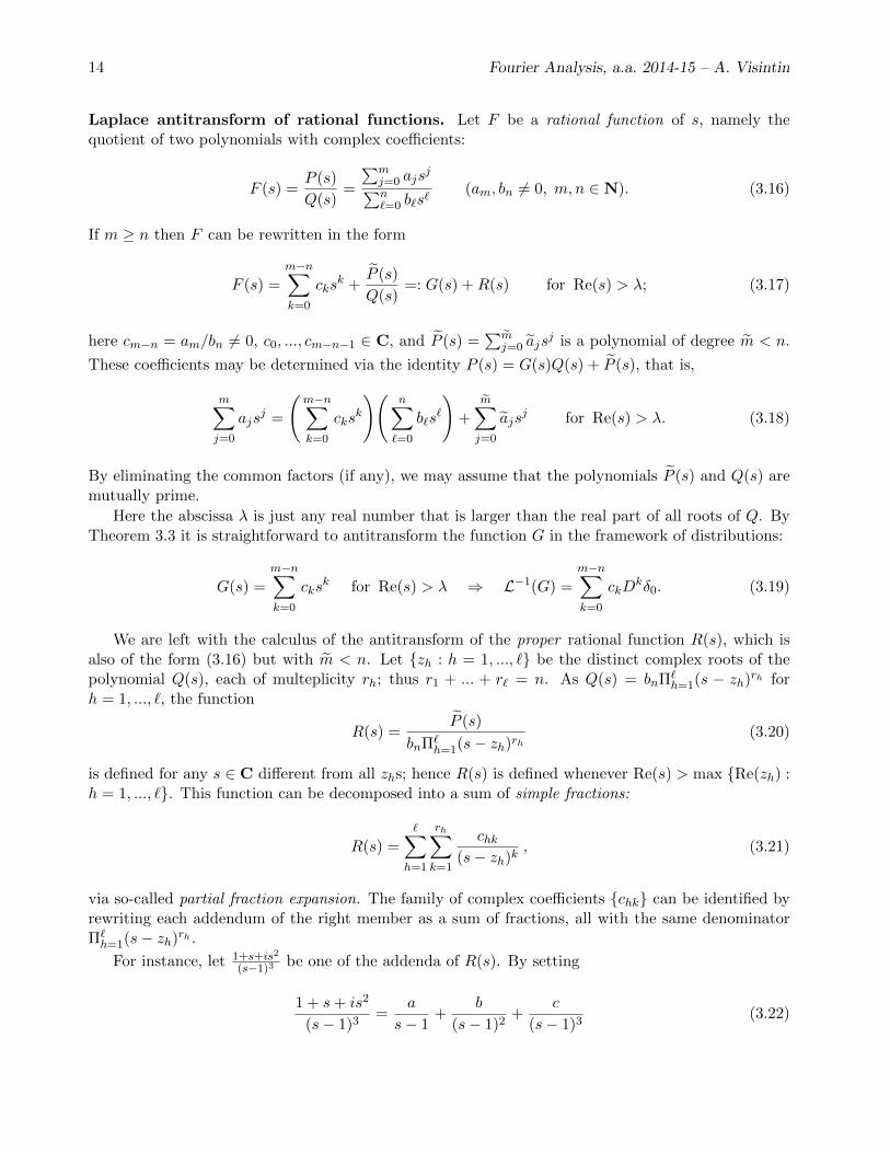
Laplace antitransform of rational functions. Let F be a rational function of s, namely thequotient of two polynomials with complex coefficients:
F (s) =P (s)
Q(s)=
∑mj=0 ajs
j∑n`=0 b`s
`(am, bn 6= 0, m, n ∈ N). (3.16)
If m ≥ n then F can be rewritten in the form
F (s) =m−n∑k=0
cksk +
P (s)
Q(s)=: G(s) +R(s) for Re(s) > λ; (3.17)
here cm−n = am/bn 6= 0, c0, ..., cm−n−1 ∈ C, and P (s) =∑m
j=0 ajsj is a polynomial of degree m < n.
These coefficients may be determined via the identity P (s) = G(s)Q(s) + P (s), that is,
m∑j=0
ajsj =
(m−n∑k=0
cksk
)(n∑`=0
b`s`
)+
m∑j=0
ajsj for Re(s) > λ. (3.18)
By eliminating the common factors (if any), we may assume that the polynomials P (s) and Q(s) aremutually prime.
Here the abscissa λ is just any real number that is larger than the real part of all roots of Q. ByTheorem 3.3 it is straightforward to antitransform the function G in the framework of distributions:
G(s) =m−n∑k=0
cksk for Re(s) > λ ⇒ L−1(G) =
m−n∑k=0
ckDkδ0. (3.19)
We are left with the calculus of the antitransform of the proper rational function R(s), which isalso of the form (3.16) but with m < n. Let {zh : h = 1, ..., `} be the distinct complex roots of thepolynomial Q(s), each of multeplicity rh; thus r1 + ... + r` = n. As Q(s) = bnΠ`
h=1(s − zh)rh forh = 1, ..., `, the function
R(s) =P (s)
bnΠ`h=1(s− zh)rh
(3.20)
is defined for any s ∈ C different from all zhs; hence R(s) is defined whenever Re(s) > max {Re(zh) :h = 1, ..., `}. This function can be decomposed into a sum of simple fractions:
R(s) =∑h=1
rh∑k=1
chk(s− zh)k
, (3.21)
via so-called partial fraction expansion. The family of complex coefficients {chk} can be identified byrewriting each addendum of the right member as a sum of fractions, all with the same denominatorΠ`h=1(s− zh)rh .
For instance, let 1+s+is2
(s−1)3be one of the addenda of R(s). By setting
1 + s+ is2
(s− 1)3=
a
s− 1+
b
(s− 1)2+
c
(s− 1)3(3.22)

Laplace transform 15
with a, b, c ∈ C to be determined, we get
1 + s+ is2
(s− 1)3=a(s− 1)2 + b(s− 1) + c
(s− 1)3=as2 − 2as+ a+ bs− b+ c
(s− 1)3(3.23)
whence a = i, b = 1 + 2i, c = 2 + i.
By (1.21) and (1.26),
L( tk−1
(k − 1)!eztH(t)
)=
1
(s− z)k∀z ∈ C, ∀k ∈ N \ {0}; (3.24)
by antitransforming (3.21) one then gets the formula
[L−1(R)](t) =∑h=1
rh∑k=1
chktk−1
(k − 1)!ezhtH(t) ∀t > 0. (3.25)
We have thus proved the following result.
Theorem 3.4. (of Heaviside) The quotient of any pair of polynomials, F (s) = P (s)Q(s) (cf. (3.16)), is
the Laplace transform of the distribution T = L−1(G) +L−1(R), see (3.19) and (3.25). T is a regulardistribution (i.e., a function) iff the degree of P (s) is strictly smaller than that of Q(s).
* Heaviside formula for simple roots. Let us assume that all the roots zh of the polynomial Q(s)are simple, i.e., Q(s) = bnΠn
n=1(s− zh), so that the expansion in simple fractions of R reads
R(s) =P (s)
Q(s)=
n∑h=1
µhs− zh
. (3.26)
Next we identify the complex coefficients µ1, ..., µn. For any k, as Q(zk) = 0 we have
R(s)(s− zk) =P (s)
[Q(s)−Q(zk)]/(s− zk)= µk +
∑h6=k
µhs− zh
(s− zk) for k = 1, ..., n. (3.27)
By passing to the limit as s→ zk, we get
lims→zk
R(s)(s− zk) =P (zk)
Q′(zk)= µk for k = 1, ..., n. (3.28)
The formula (3.26) thus yields the following classical result.
Theorem 3.5. (Heaviside formula) If the roots zh of the polynomial Q(s) are all simple, then
[L−1(P /Q)](t) =n∑h=1
P (zh)
Q′(zh)ezhtH(t) ∀t > 0. (3.29)
* Case of multiple roots. For instance, let us assume that Q(s) = (s− z)r for some z ∈ C and aninteger r ≥ 1, and let us look for an expansion in simple fractions of the form (3.26). As
[Dr−ks (s− zh)rR(s)]s=zh = (r − k)!chk for k = 1, ..., r, h = 1, ..., `, (3.30)
16 Fourier Analysis, a.a. 2014-15 – A. Visintin
we can identify the complex coefficients of (3.25):
chk =1
(r − k)![Dr−k
s (s− zh)rR(s)]s=zh for k = 1, ..., r, h = 1, ..., `. (3.31)
Exercises— Check that the function L−1(R) is bounded if Re(zh) < 0 for any h, and that if L−1(R) is
bounded then Re(zh) ≤ 0 for any h.— Check u ∗Dnδ0 = Dnu for any u ∈ L1
loc and any n ∈ N.
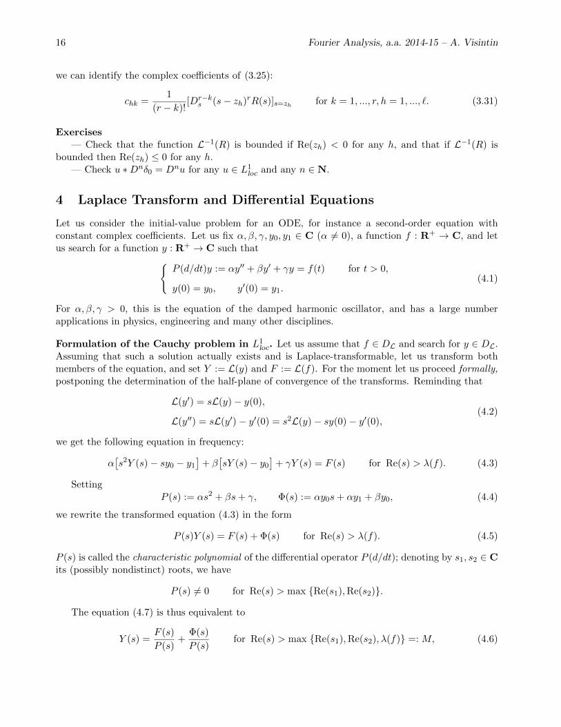
4 Laplace Transform and Differential Equations
Let us consider the initial-value problem for an ODE, for instance a second-order equation withconstant complex coefficients. Let us fix α, β, γ, y0, y1 ∈ C (α 6= 0), a function f : R+ → C, and letus search for a function y : R+ → C such that{
P (d/dt)y := αy′′ + βy′ + γy = f(t) for t > 0,
y(0) = y0, y′(0) = y1.(4.1)
For α, β, γ > 0, this is the equation of the damped harmonic oscillator, and has a large numberapplications in physics, engineering and many other disciplines.
Formulation of the Cauchy problem in L1loc. Let us assume that f ∈ DL and search for y ∈ DL.
Assuming that such a solution actually exists and is Laplace-transformable, let us transform bothmembers of the equation, and set Y := L(y) and F := L(f). For the moment let us proceed formally,postponing the determination of the half-plane of convergence of the transforms. Reminding that
L(y′) = sL(y)− y(0),
L(y′′) = sL(y′)− y′(0) = s2L(y)− sy(0)− y′(0),(4.2)
we get the following equation in frequency:
α[s2Y (s)− sy0 − y1
]+ β
[sY (s)− y0
]+ γY (s) = F (s) for Re(s) > λ(f). (4.3)
SettingP (s) := αs2 + βs+ γ, Φ(s) := αy0s+ αy1 + βy0, (4.4)
we rewrite the transformed equation (4.3) in the form
P (s)Y (s) = F (s) + Φ(s) for Re(s) > λ(f). (4.5)
P (s) is called the characteristic polynomial of the differential operator P (d/dt); denoting by s1, s2 ∈ Cits (possibly nondistinct) roots, we have
P (s) 6= 0 for Re(s) > max {Re(s1),Re(s2)}.
The equation (4.7) is thus equivalent to
Y (s) =F (s)
P (s)+
Φ(s)
P (s)for Re(s) > max {Re(s1),Re(s2), λ(f)} =: M, (4.6)
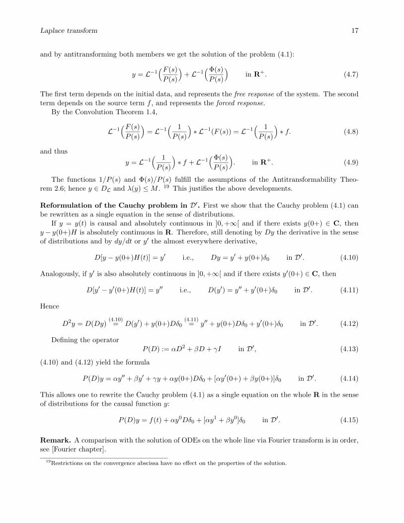
Laplace transform 17
and by antitransforming both members we get the solution of the problem (4.1):
y = L−1(F (s)
P (s)
)+ L−1
(Φ(s)
P (s)
)in R+. (4.7)
The first term depends on the initial data, and represents the free response of the system. The secondterm depends on the source term f , and represents the forced response.
By the Convolution Theorem 1.4,
L−1(F (s)
P (s)
)= L−1
( 1
P (s)
)∗ L−1(F (s)) = L−1
( 1
P (s)
)∗ f. (4.8)
and thus
y = L−1( 1
P (s)
)∗ f + L−1
(Φ(s)
P (s)
). in R+. (4.9)
The functions 1/P (s) and Φ(s)/P (s) fulfill the assumptions of the Antitransformability Theo-rem 2.6; hence y ∈ DL and λ(y) ≤M . 19 This justifies the above developments.
Reformulation of the Cauchy problem in D′. First we show that the Cauchy problem (4.1) canbe rewritten as a single equation in the sense of distributions.
If y = y(t) is causal and absolutely continuous in ]0,+∞[ and if there exists y(0+) ∈ C, theny− y(0+)H is absolutely continuous in R. Therefore, still denoting by Dy the derivative in the senseof distributions and by dy/dt or y′ the almost everywhere derivative,
D[y − y(0+)H(t)] = y′ i.e., Dy = y′ + y(0+)δ0 in D′. (4.10)
Analogously, if y′ is also absolutely continuous in ]0,+∞[ and if there exists y′(0+) ∈ C, then
D[y′ − y′(0+)H(t)] = y′′ i.e., D(y′) = y′′ + y′(0+)δ0 in D′. (4.11)
Hence
D2y = D(Dy)(4.10)
= D(y′) + y(0+)Dδ0(4.11)
= y′′ + y(0+)Dδ0 + y′(0+)δ0 in D′. (4.12)
Defining the operator
P (D) := αD2 + βD + γI in D′, (4.13)
(4.10) and (4.12) yield the formula
P (D)y = αy′′ + βy′ + γy + αy(0+)Dδ0 + [αy′(0+) + βy(0+)]δ0 in D′. (4.14)
This allows one to rewrite the Cauchy problem (4.1) as a single equation on the whole R in the senseof distributions for the causal function y:
P (D)y = f(t) + αy0Dδ0 + [αy1 + βy0]δ0 in D′. (4.15)
Remark. A comparison with the solution of ODEs on the whole line via Fourier transform is in order,see [Fourier chapter].
19Restrictions on the convergence abscissa have no effect on the properties of the solution.

18 Fourier Analysis, a.a. 2014-15 – A. Visintin
Use of the Laplace transform in D′. As we just saw, distributions allow one to include the initialdata into the forcing term. This allows us to provide a more synthetical approach to the Cauchyproblem.
The second member of the equation (4.7) reads
G(s) := F (s) + Φ(s) = F (s) + αy0s+ αy1 + βy0 for Re(s) > λ(f). (4.16)
Notice that by transforming the equation (4.15) the same result is obtained.The equation (4.7) also reads P (s)Y (s) = G(s), and has the solution
Y (s) =G(s)
P (s)for Re(s) > max {Re(s1),Re(s2), λ(f)}. (4.17)
Let us apply the antitransform L−1 to this equality. Recalling that
λ(Dnδ0) = −∞, L(Dnδ0) = sn ∀n ∈ N, (4.18)
we haveL−1(αy0s+ αy1 + βy0) = αy0Dδ0 + (αy1 + βy0). (4.19)
Setting h = L−1(1/P (s)), we thus get the solution of problem (4.1) in the sense of distributions:
y = L−1( 1
P (s)(F + Φ)
)= L−1
( 1
P (s)
)∗ [L−1(F ) + L−1(Φ)]
= h ∗ [f + αy0Dδ0 + (αy1 + βy0)δ0]
= h ∗ f + αy0Dh+ (αy1 + βy0)h in R+.
(4.20)
We thus retrieved (4.9), and obtained a more explicit representation of the solution.
The transfer function. The approach of the linear system theory can be applied to initial-valueproblems via the Laplace transform, along a line that is reminiscent of what we saw for differentialequations on the whole R via the Fourier transform. In this case the solution y linearly depends onthe initial data y0, y1 and on the forcing term f . This is more clear by using the Laplace transform inD′.
Let us first assume thaty0 = y1 = 0, (4.21)
so that the system that maps the input f to the output u is linear (rather than affine). 20 In theterminology of system theory, the solution operator L : f 7→ y is called a continuous filter. Here wejust deal with the filter that is associated to problem (4.1); however this analysis can be extended tohigher order problems, and to a much more general set-up — including partial differential equations,integro-differential equations, and so on.
Let h := L(δ0) be the response in time to the unit impulse δ0, that is,
(P (D)h :=) αD2h+ βDh+ γh = δ0 in D′(R), (4.22)
or also, because of (4.9),
h = L−1( 1
P (s)
)∗ δ0 = L−1
( 1
P (s)
) (∈ DL). (4.23)
20 If the initial data are not homogeneous, however via the approach of distributions we can retrieve a linear systemby including the initial data into the forcing term.
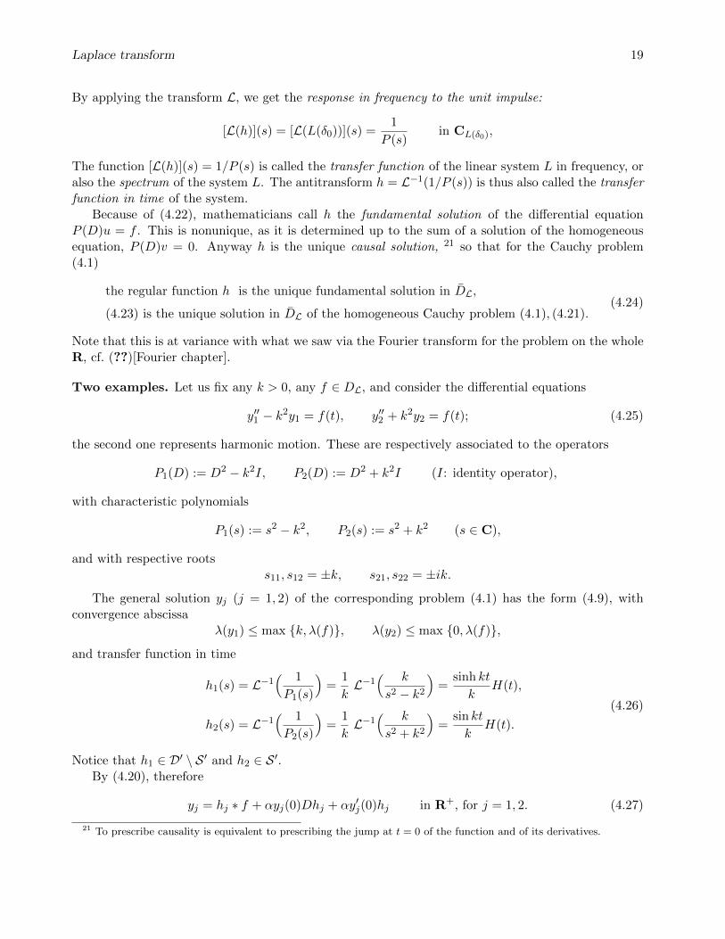
Laplace transform 19
By applying the transform L, we get the response in frequency to the unit impulse:
[L(h)](s) = [L(L(δ0))](s) =1
P (s)in CL(δ0),
The function [L(h)](s) = 1/P (s) is called the transfer function of the linear system L in frequency, oralso the spectrum of the system L. The antitransform h = L−1(1/P (s)) is thus also called the transferfunction in time of the system.
Because of (4.22), mathematicians call h the fundamental solution of the differential equationP (D)u = f . This is nonunique, as it is determined up to the sum of a solution of the homogeneousequation, P (D)v = 0. Anyway h is the unique causal solution, 21 so that for the Cauchy problem(4.1)
the regular function h is the unique fundamental solution in DL,
(4.23) is the unique solution in DL of the homogeneous Cauchy problem (4.1), (4.21).(4.24)
Note that this is at variance with what we saw via the Fourier transform for the problem on the wholeR, cf. (??)[Fourier chapter].
Two examples. Let us fix any k > 0, any f ∈ DL, and consider the differential equations
y′′1 − k2y1 = f(t), y′′2 + k2y2 = f(t); (4.25)
the second one represents harmonic motion. These are respectively associated to the operators
P1(D) := D2 − k2I, P2(D) := D2 + k2I (I: identity operator),
with characteristic polynomials
P1(s) := s2 − k2, P2(s) := s2 + k2 (s ∈ C),
and with respective rootss11, s12 = ±k, s21, s22 = ±ik.
The general solution yj (j = 1, 2) of the corresponding problem (4.1) has the form (4.9), withconvergence abscissa
λ(y1) ≤ max {k, λ(f)}, λ(y2) ≤ max {0, λ(f)},
and transfer function in time
h1(s) = L−1( 1
P1(s)
)=
1
kL−1
( k
s2 − k2
)=
sinh kt
kH(t),
h2(s) = L−1( 1
P2(s)
)=
1
kL−1
( k
s2 + k2
)=
sin kt
kH(t).
(4.26)
Notice that h1 ∈ D′ \ S ′ and h2 ∈ S ′.By (4.20), therefore
yj = hj ∗ f + αyj(0)Dhj + αy′j(0)hj in R+, for j = 1, 2. (4.27)
21 To prescribe causality is equivalent to prescribing the jump at t = 0 of the function and of its derivatives.

20 Fourier Analysis, a.a. 2014-15 – A. Visintin
* Higher-order equations. The previous analysis can be extended to initial-value problems forequations of any order M ≥ 1.
Let α0, ..., αM , y0, ..., yM−1 ∈ C (αM 6= 0), f : R+ → C, and let us search for y : R+ → C suchthat
M∑m=0
αmDmy = f(t) for t > 0
Dmy(0) = ym for m = 0, ...,M − 1.
(4.28)
Let us assume that f, y ∈ DL, set Y := L(y) and F := L(f), and apply the Laplace transform to(4.28). Recalling the differentiation Theorem 2.2, (4.28) yields
M∑m=0
αmsmY (s)−
M∑m=0
αm
m−1∑n=0
sm−1−nyn = F (s) for Re(s) > max {M,λ(f)}. (4.29)
(As we saw for the second-order equation, here also we might formulate the Cauchy problem as a singleequation in the sense of distributions, getting of course the same transformed equation.) Defining
P (s) :=M∑m=0
αmsm (characteristic polynomial),
Φ(s) :=M∑m=0
αm
m−1∑n=0
sm−1−nyn,
(4.30)
the equation (4.29) reads
P (s)Y (s) = F (s) + Φ(s) for Re(s) > λ(f). (4.31)
Denoting by s1, ..., sN ∈ C the (possibly nondistinct) complex roots of P (s),
P (s) 6= 0 for Re(s) > M := max {Re(si) : i = 1, ..., N}.
The equation (4.29) is thus equivalent to
Y (s) =F (s)
P (s)+
Φ(s)
P (s)for Re(s) > max {M,λ(f)}.
Defining the transfer function in time h := L−1(1/P (s)), the Convolution Theorem 1.4 and (4.30)2
yield
y = L−1( 1
P (s)F)
+ L−1( 1
P (s)Φ)
= h ∗ L−1(F ) + h ∗ L−1(Φ)
= h ∗ f +M∑m=0
αm
m−1∑n=0
yn h ∗Dm−1−nδ0
= h ∗ f +M∑m=0
αm
m−1∑n=0
yn Dm−1−nh in R+.
(4.32)
This is the sum of the free and forced responses. The function y has convergence abscissa λ(y) ≤max {M,λ(f)}. This justifies the previous transformations.
Laplace transform 21
This discussion can be extended in several directions: e.g., the Cauchy problem for systems ofdifferential equations, equations and systems of differential equations with delay, and so on.
* Linear systems of first-order equations. Let
A ∈ CN×N (N ≥ 1), f : R+ → CN , f ∈ L1loc, u0 ∈ CN ,
and consider the following first-order vectorial Cauchy problem, for the unknown function u : R+ →CN : {
Dtu = A · u+ f in R+,
u(0) = u0.(4.33)
By extending u and f to causal (vectorial) functions, this problem can be formulated as the singleequation
Dtu = A · u+ f + u0δ0 in D′(R)N . (4.34)
Let us assume that f and u are both Laplace-transformable (componentwise), and set U = L(u),F = L(f). By transforming the equation (4.34), we get
(sI −A) · U(s) = F (s) + u0 for Re(s) > maxj=1,...,N
{λ(uj), λ(fj)}, (4.35)
that is, defining the resolvent matrix R(s) = (sI −A)−1,
U(s) = R(s) · [F (s) + u0] for Re(s) large enough. (4.36)
More precisely, defining the (possibly nondistinct) complex eigenvalues s1, ..., sN of the matrix A,(4.36) holds for Re(s) > maxj=1,...,N {λ(uj), λ(fj),Re(sj)}.
Let us now introduce the (causal) matrix antitransform S = L−1(R) : R → CN×N , namely, thesolution of the problem
(sI −A)−1 = [L(S)](s) for Re(s) > maxj=1,...,N
{Re(sj)}. (4.37)
Antitransforming the equation (4.36) we get u(t) = L−1(R) ∗ L−1(F + u0). We thus retrieve theclassical formula of variation of parameters:
u(t) = S(t) ∗ f(t) + S(t) ∗ (u0δ0) =
∫ t
0S(t− τ) · f(τ) dτ + S(t) · u0 ∀t ∈ R. (4.38)
The function S represents the semigroup that is determined by the matrix A. 22 The equations(4.37) and (4.38) can then be interpreted as
the resolvent (sI −A)−1 of the semigroup S(t)
coincides with the Laplace transform of that semigroup.(4.39)
Notice that, using the definition of exponential of a matrix,
S(t) = eAtH(t) =∞∑n=0
Antn
n!H(t) (∈ CN×N ) ∀t ∈ R. (4.40)
22 A semigroup is a family of operators S : [0,+∞[→ L(X) (L(X) being the space of linear and continuous operatorson a Banach space X) such that S(t1 + t2) = S(t1) ◦ S(t2) for any t1, t2 ≥ 0.

22 Fourier Analysis, a.a. 2014-15 – A. Visintin
* Linear systems of higher-order equations. Let A, f be as above, m ∈ N, an, un ∈ C for
n = 0, ...,m− 1 (am 6= 0), and consider the following vector Cauchy problem of order m:{ ∑mn=0 anD
nu(t) = A · u(t) + f(t) for t > 0,
Dnu(0) = un for n = 0, ...,m− 1.(4.41)
By extending u and f to causal vector functions, this problem can be formulated as the single vectorequation
m∑n=0
anDnu(t) = A · u(t) + f(t) +
m−1∑n=0
anunDm−1−nδ0 in D′(R)N . (4.42)
Let us assume that f, y ∈ DL, set U = L(u) and F = L(f); let us also define the characteristicpolynomial P (s) and the polynomial Φ(s) as follows:
P (s) =
m∑n=0
ansn, Φ(s) =
m∑n=1
n−1∑j=0
anujsn−h−1 ∀s ∈ C. (4.43)
By transforming the equation (4.43), we get
[P (s)I −A] · U(s) = F (s) + Φ(s) for Re(s) > max {λ(u), λ(f)}, (4.44)
that is, defining the matrix function R(s) = [P (s)I −A]−1,
U(s) = R(s) · [F (s) + Φ(s)] for Re(s) large enough. (4.45)
Let us introduce the matrix antitransform S = L−1(R) : R → CN×N , that is, the solution of theproblem
[P (s)I −A]−1 = [L(S)](s) for Re(s) large enough. (4.46)
Antitransforming the (4.45), we get
u = S ∗ f + S ∗ L−1(Φ) = S ∗ f + S ∗m∑n=1
n−1∑j=0
anujDn−h−1h in R. (4.47)
This approach can be extended to linear evolutionary PDEs, e.g. of the form Dtu + Au = f ; inthis case the associated stationary operator A, in an infinite-dimensional space (typically a Sobolevspace).