P.S. GandhiP.S. GandhiMechanical Engineering Mechanical Engineering IIT BombayIIT Bombay

LaplaceLaplace Transforms and use Transforms and use in Automatic Controlin Automatic Control

Acknowledgements: P.Santosh Krishna, SYSCON

Recap

Fourier seriesFourier seriesFourier transform: Fourier transform: aperiodicaperiodicConvolution integralConvolution integralFrequency responseFrequency response

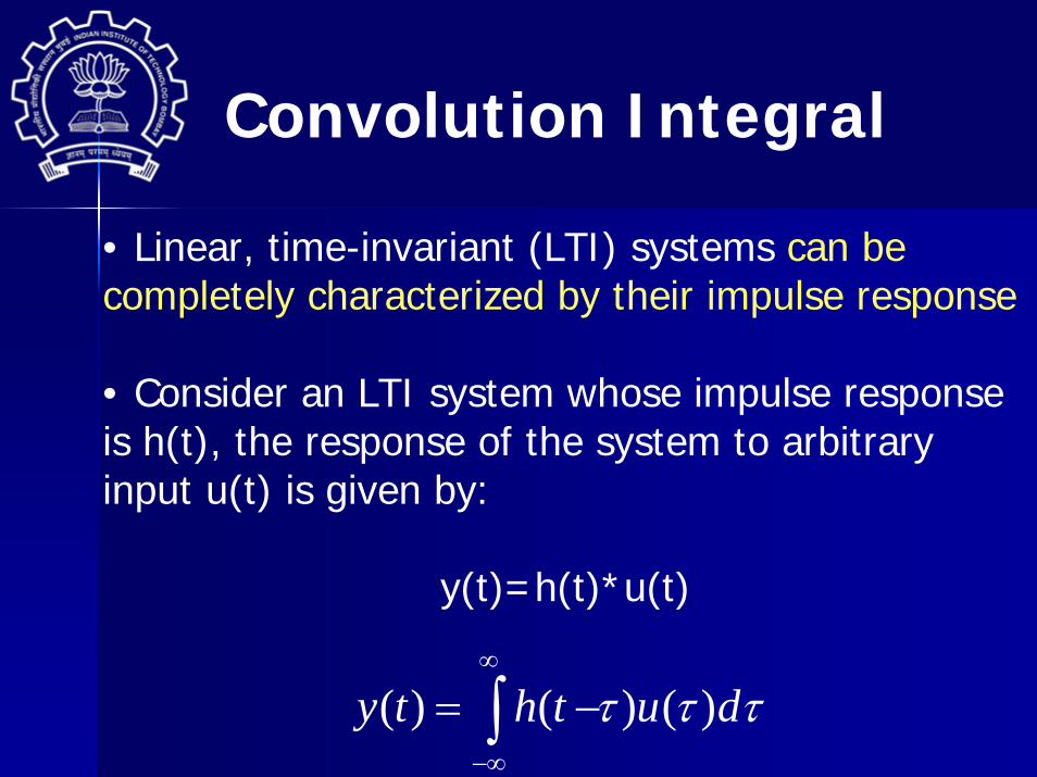
Convolution Integral

• Linear, time-invariant (LTI) systems can be completely characterized by their impulse response

• Consider an LTI system whose impulse response is h(t), the response of the system to arbitrary input u(t) is given by:

y(t)=h(t)*u(t)

( ) ( ) ( )y t h t u dτ τ τ∞

−∞

= −∫

Convolution Integral Fundamentals

Convolution as sumof inverted and shiftedimpulse responsesat various input points

Frequency Response

LTIe jωt ?

Frequency response of the system = fourier transform of the impulse response

H(jω) e jωt

Complex Exponentials and LTI systems

LTIe jωt ? H(jω) e jωt

What will be the response of the system to a sum of complex exponentials?

Integration and differentiation can be replaced by Integration and differentiation can be replaced by algebraic operations in complex plane.algebraic operations in complex plane.It converts complex functions such as sinusoidal, It converts complex functions such as sinusoidal, exponential into algebraic functions of complex exponential into algebraic functions of complex variable variable ‘‘ss’’These algebraic equations can be easily solved in These algebraic equations can be easily solved in ‘‘ss’’ for dependent variable whose time domain for dependent variable whose time domain response can be found with inverse response can be found with inverse LaplaceLaplacetransformstransforms

Q: cant we do these by using Fourier transform?Q: cant we do these by using Fourier transform?A: Not always. We will consider some cases laterA: Not always. We will consider some cases later

Why Laplace transforms ??

MA 203

Definition of L.T.

If is a function of time , forIf is a function of time , forand and ‘‘ss’’ is a complex variable is a complex variable and F(s) is the laplace transform of functionand F(s) is the laplace transform of function

Then the laplace transform of is given by,Then the laplace transform of is given by,

What if s = What if s = jwjw ????? ?????

( )f t ( ) 0f t = 0t <

( )f t

( )f t

( )0

( ) ( ). stF s L f t f t e dt∞

−= =⎡ ⎤⎣ ⎦ ∫

Fourier transformformula

Inverse Laplace Transforms

If F(s) is the laplace transform of a function,If F(s) is the laplace transform of a function,then its time domain response is given bythen its time domain response is given by

for for

This is called inverse This is called inverse LaplaceLaplace transform of F(s)transform of F(s)

( )1 1( ) ( )2

c jst

c j

L F s f t F s e dsjπ

+ ∞−

− ∞

⎡ ⎤ = =⎣ ⎦ ∫0t >

We have already seen Fourier transform which is a We have already seen Fourier transform which is a function of the complex variable . Laplace transfunction of the complex variable . Laplace trans--form is a function of the complex variable form is a function of the complex variable ‘‘ss’’ denoting denoting

in which if = 0, then in which if = 0, then LaplaceLaplace transforms transforms equals Fourier transforms.equals Fourier transforms.What does this mean physically??? What does this mean physically???

LaplaceLaplace transforms are introduced to fill the gaps transforms are introduced to fill the gaps which Fourier transform does not; We see which Fourier transform does not; We see these two cases with examples. these two cases with examples.

jw

' '

Advantages of L.T over F.T

jwσ + σ

Case 1Case 1: Unstable systems: Unstable systemsStable system is one which gives bounded output Stable system is one which gives bounded output

for bounded input. Consider the unstable systemfor bounded input. Consider the unstable systemwhose output diverge for a unit step whose output diverge for a unit step

input.input.Applying Fourier transforms on both sides, we getApplying Fourier transforms on both sides, we get

( ) ( ).y t t u t=

( ) ( ). jwtY jw tu t e dt∞

−

−∞

⎡ ⎤= ⎢ ⎥⎣ ⎦∫

Advantages of L.T over F.T

which is violated in this case. Thus, it is clear that wewhich is violated in this case. Thus, it is clear that wecancan’’t find Fourier transform for unstable systems. Now, t find Fourier transform for unstable systems. Now, taking Laplace transforms,taking Laplace transforms,

But But DirichletsDirichlets first condition states that [t.u(t)] should first condition states that [t.u(t)] should be absolutely integrable for the Fourier transform to be absolutely integrable for the Fourier transform to exist. That is, exist. That is,

| ( ) |tu t dt∞

−∞

< ∞∫

Advantages of L.T over F.T

( ) ( ). stY s tu t e dt∞

−

−∞

= ∫

0

. stt e dt∞

−= ∫ 20

. st stt e es s

∞− −⎡ ⎤= − −⎢ ⎥⎣ ⎦

2

1s

= for Re{s}> 0for Re{s}> 0

So, it is clear that for unstable systems, even thoughSo, it is clear that for unstable systems, even thoughFourier transform does not exist, Fourier transform does not exist, LaplaceLaplace transform transform exits which helps to investigate the stability of a systemexits which helps to investigate the stability of a system

Advantages of L.T over F.T

Case 2Case 2::Let us take the input signal as below instead of unit stepLet us take the input signal as below instead of unit step

Since we need to find F.T of both the system and theSince we need to find F.T of both the system and theinput signal in order to obtain the output response, weinput signal in order to obtain the output response, weneed to find F.T of this input signal given aboveneed to find F.T of this input signal given above

( ) . ( )atx t e u t=

( ) ( ).at jwtX jw e u t e dt∞

−

−∞

= ∫

Advantages of L.T over F.T

( )0

at jwtX jw e dt∞

−⇒ = ∫The right side part is tending to infinite, so we canThe right side part is tending to infinite, so we can’’t t find F.T for this input signal. We can conclude thisfind F.T for this input signal. We can conclude thiswithout any calculations directly from Dirichlet firstwithout any calculations directly from Dirichlet firstcondition as in casecondition as in case--1. Taking Laplace transforms,1. Taking Laplace transforms,

( ) ( ).at stX s e u t e dt∞

−

−∞

= ∫

Advantages of L.T over F.T

( ) ( )

0

t s aX s e dt∞

− −⇒ = ∫1

s a=

−forfor

So, for some values of Re{s}, we are able to find L.TSo, for some values of Re{s}, we are able to find L.Tfor the given signal. This is called for the given signal. This is called ‘‘Region of ConvergencRegion of Convergenc(ROC). Here, it is the area in s(ROC). Here, it is the area in s--plane whose real part is plane whose real part is greater than greater than ‘‘aa’’. In case. In case--1, ROC in the right half of the1, ROC in the right half of theSS--plane.plane.

{ }Re s a>

Advantages of L.T over F.T

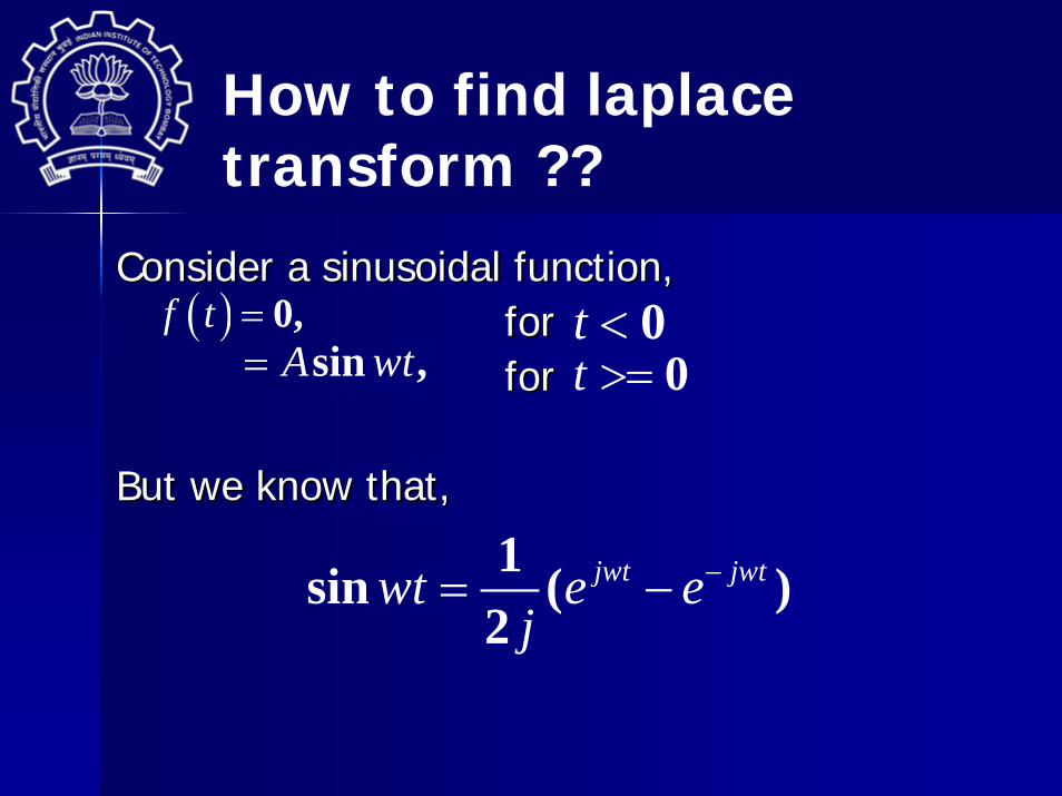
How to find laplace transform ??

Consider a sinusoidal function,Consider a sinusoidal function,for for forfor

But we know that,But we know that,

( ) 0,f t = 0t <sin ,A wt= 0t >=

1sin ( )2

jwt jwtwt e ej

−= −

contd…….

Hence Hence

[ ]0

sin ( )2

jwt jwt stAL A wt e e e dtj

∞− −= −∫

1 1. .2 2A Aj s jw j s jw

= −− +

2 2

Aws w

=+

FunctionFunction TransformTransformUnit impulse 1Unit impulse 1Unit step Unit step

Laplace transforms for some commonly used functions

nt 1

!n

ns +

ate− 1s a+

sin wt 2 2

ws w+

1/ s

FunctionFunction TransformTransform

cos wt 2 2

ss w+

sinh wt 2 2

ws w−

cosh wt 2 2

ss w−

contd…….

Some other functionsSome other functions

Observe how affects these functions,Observe how affects these functions,FunctionFunction TransformTransform

ate−

1

!( )n

ns a ++

sinate wt−2 2( )

ws a w+ +

cosate wt−2 2( )

s as a w

++ +

at ne t−

Contd…….

FunctionFunction TransformTransform

i.e, i.e,

( )0

. . ( ). ( )at at stL e f t e f t e dt F s a∞

− − −⎡ ⎤ = = +⎣ ⎦ ∫

sinhate wt−2 2( )

ws a w+ −

coshate wt−

2 2( )s a

s a w+

+ −

L.T of a translated functionL.T of a translated function

let F(s) be the L.T of f(t) and l(t) is a functionlet F(s) be the L.T of f(t) and l(t) is a functionsuch that such that

for for t α<( ). ( ) 0f t l tα α− − =

Contd…….

then L.T of is given by,then L.T of is given by,( ). ( )f t u tα α− −

0

[ ( ). ( )] ( ) ( ). stL f t l t f t l t e dtα α α α∞

−− − = − −∫

( )( ) ( ) . s tf t l t e d tα

α

∞− +

−

= ∫

0

( ) . .s t tf t e e d tα∞

− −= ∫

. ( )se F sα−=

Change of time scaleChange of time scale

If If ‘‘tt’’ is changed intois changed into where is a where is a positive constant. Then function has positive constant. Then function has changed into then L.T of changed into then L.T of is,is,

/ ,t α α( )f t

,tfα⎛ ⎞⎜ ⎟⎝ ⎠

tfα⎛ ⎞⎜ ⎟⎝ ⎠

0

. stt tL f f e d tα α

∞−⎡ ⎤⎛ ⎞ ⎛ ⎞=⎜ ⎟ ⎜ ⎟⎢ ⎥⎝ ⎠ ⎝ ⎠⎣ ⎦

∫

( )0

. . stf t e dtαα∞

−= ∫ ( )F sα α=

Laplace transform theoremsLaplace transform theorems

Real differentiation theoremReal differentiation theorem

Real integration theoremReal integration theorem

Complex differentiation theoremComplex differentiation theorem

( ) ( ) (0)dL f t sF s fdt⎡ ⎤ = −⎢ ⎥⎣ ⎦

1( ) (0)( ) F s fL f t dts s

−

⎡ ⎤ = +⎣ ⎦∫

( ). ( )dL t f t F sds

= −⎡ ⎤⎣ ⎦

IMP for LTI

From this theorem, we can find the value of From this theorem, we can find the value of f(t) at t=0+ directly from the L.T of f(t).f(t) at t=0+ directly from the L.T of f(t).This theorem will not give the value of f(t) This theorem will not give the value of f(t) exactly at t=0 but slightly greater than zeroexactly at t=0 but slightly greater than zero

DefDef: If f(t) and are laplce transformable: If f(t) and are laplce transformableand if exists then,and if exists then,

Initial value theoremInitial value theorem

( )df tdt

lim ( )s

sF s→∞

(0 ) lim ( )s

f sF s→∞

+ =

Final value theorem

This theorem gives the value of f(t) when This theorem gives the value of f(t) when This theorem applies if and only if exitsThis theorem applies if and only if exitsAll the poles of should lie in the left half of All the poles of should lie in the left half of ss--plane for to exist.plane for to exist.

DefDef: If f(t) and are laplce transformable: If f(t) and are laplce transformableand if exists then, and if exists then,

t →∞lim ( )t

f t→∞

lim ( )t

f t→∞

( )sF s

( )df tdt

lim ( )t

f t→∞

0lim ( ) lim ( )t s

f t sF s→∞ →

=

Convolution IntegralConvolution Integral

The integral can also be The integral can also be written as which is known as written as which is known as convolution integral.convolution integral.If & are L.TIf & are L.T’’s of & s of & respectively, then L.T of convolution respectively, then L.T of convolution integral is given by,integral is given by,

1 20

( ) ( )t

f t f dτ τ τ−∫1 2( ) ( )f t f t∗

1( )F s 2 ( )F s 2 ( )f t1( )f t

1 1 1 20

( ) ( ) ( ). ( )t

L f t f t d F s F sτ τ⎡ ⎤

− =⎢ ⎥⎣ ⎦∫

Blocks can be multiplicative in Laplace domain

L.T of product of two L.T of product of two time functionstime functions

If F(s) and G(s) are the laplace transforms If F(s) and G(s) are the laplace transforms of f(t) and g(t) respectively, then the of f(t) and g(t) respectively, then the laplace transform of is given by,laplace transform of is given by,( ) ( )f t g t∗

[ ] 1( ) ( ) ( ). ( )2

c j

c j

L f t g t F p G s p dpjπ

+ ∞

− ∞

∗ = −∫

Example ProblemExample Problem

We have already seen block diagram representation to We have already seen block diagram representation to a system with integrators, differentiators and multiplier a system with integrators, differentiators and multiplier blocks. But this block diagram representation becomes blocks. But this block diagram representation becomes much simpler with this Laplace transforms as shown.much simpler with this Laplace transforms as shown.

Let us consider the system given in exam,Let us consider the system given in exam,

First let us find the system response applying L.TFirst let us find the system response applying L.T’’ss

.. .( ) 5 ( ) 2 ( ) 10. ( )y t y t y t x t+ + =

2 ( ) 5 . ( ) 2 ( ) 10. ( )s Y s s Y s Y s X s+ + =

Ex. Problem (ContdEx. Problem (Contd…………))

This ratio of output to input is called This ratio of output to input is called ‘‘Transfer FunctionTransfer Function’’After finding the partial fractions and applying Inverse After finding the partial fractions and applying Inverse Laplace transforms to above transfer function with unitLaplace transforms to above transfer function with unitStep as input, we get the following output,Step as input, we get the following output,

2

( ) 10( ) 5 2

Y sX s s s

⇒ =+ +

0.439 4.562( ) 2.425( ) 5 ( )t ty t e e u t− −= − +Solve and prove in class

The block diagram representation for the above system The block diagram representation for the above system with integrator and multiplier blocks is, with integrator and multiplier blocks is,

Ex. Problem (ContdEx. Problem (Contd…………))

For designing this small system, we needed manyFor designing this small system, we needed manyintegrator, gain and summation blocks leading to bigintegrator, gain and summation blocks leading to bigblock diagram. Instead, we can form it in Sblock diagram. Instead, we can form it in S--domain domain with only a single transfer function block which is with only a single transfer function block which is obtained in previous slide. obtained in previous slide.

Ex. Problem (ContdEx. Problem (Contd…………))

This reduces the complexity of the block diagram veryThis reduces the complexity of the block diagram verymuch and thus representation of much bigger plantsmuch and thus representation of much bigger plantsalso became simpler with just these transfer functionalso became simpler with just these transfer functionblocks and multiplier blocks. The output response of blocks and multiplier blocks. The output response of the system will be same in both the block diagram the system will be same in both the block diagram representations with MATLAB. These output responsesrepresentations with MATLAB. These output responsesare shown in next slide. are shown in next slide.

Ex. Problem (ContdEx. Problem (Contd…………))

Response in time domain block diagram Response in time domain block diagram

Ex. Problem (ContdEx. Problem (Contd…………))

Response in transfer function block diagramResponse in transfer function block diagram

Ex. Problem (ContdEx. Problem (Contd…………))