laplace transforms prepared by mrs. azduwin binti khasri
TRANSCRIPT

LAPLACE TRANSFORMS
Prepared by Mrs. Azduwin Binti Khasri
LAPLACE TRANSFORMS
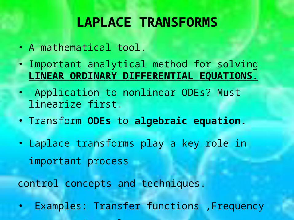
• A mathematical tool.
• Important analytical method for solving LINEAR ORDINARY DIFFERENTIAL EQUATIONS.
• Application to nonlinear ODEs? Must linearize first.
• Transform ODEs to algebraic equation.
• Laplace transforms play a key role in important process
control concepts and techniques.
• Examples: Transfer functions ,Frequency response,Control
system design, Stability analysis
3
0
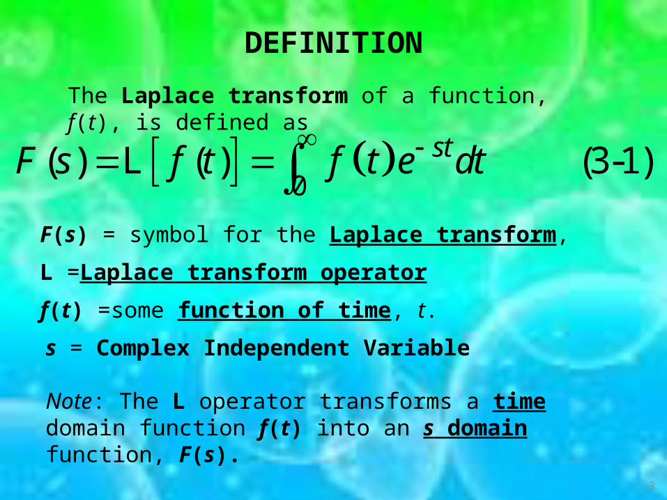
( ) ( ) (3-1)stF s f t f t e dt L
The Laplace transform of a function, f(t), is defined as
F(s) = symbol for the Laplace transform,
L =Laplace transform operator
f(t) =some function of time, t.
s = Complex Independent Variable
Note: The L operator transforms a time domain function f(t) into an s domain function, F(s).
DEFINITION
4
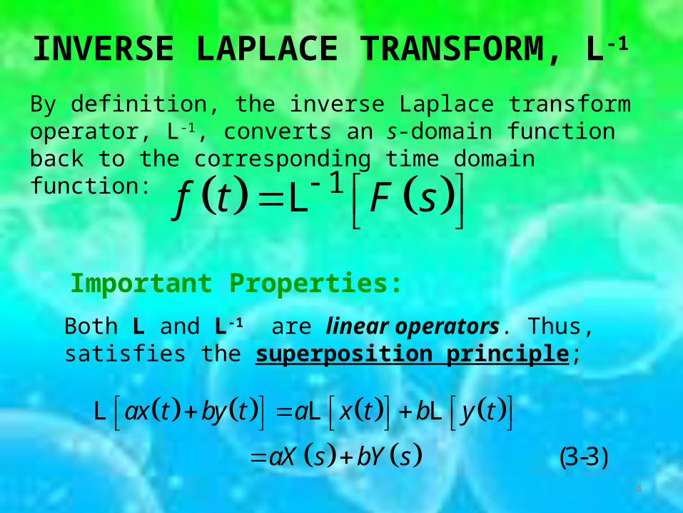
INVERSE LAPLACE TRANSFORM, L-1
By definition, the inverse Laplace transform operator, L-1, converts an s-domain function back to the corresponding time domain function:
1f t F s L
Important Properties:
Both L and L-1 are linear operators. Thus, satisfies the superposition principle;
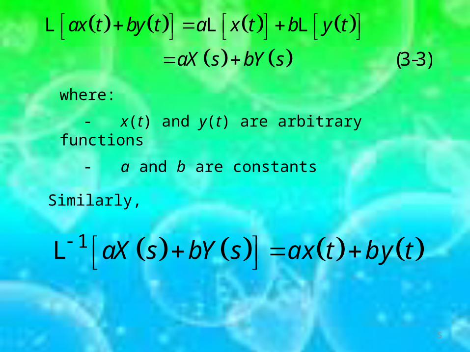
(3-3)
ax t by t a x t b y t
aX s bY s
L L L
5
where:
- x(t) and y(t) are arbitrary functions
- a and b are constants
Similarly,
1 aX s bY s ax t b y t L
(3-3)
ax t by t a x t b y t
aX s bY s
L L L
6
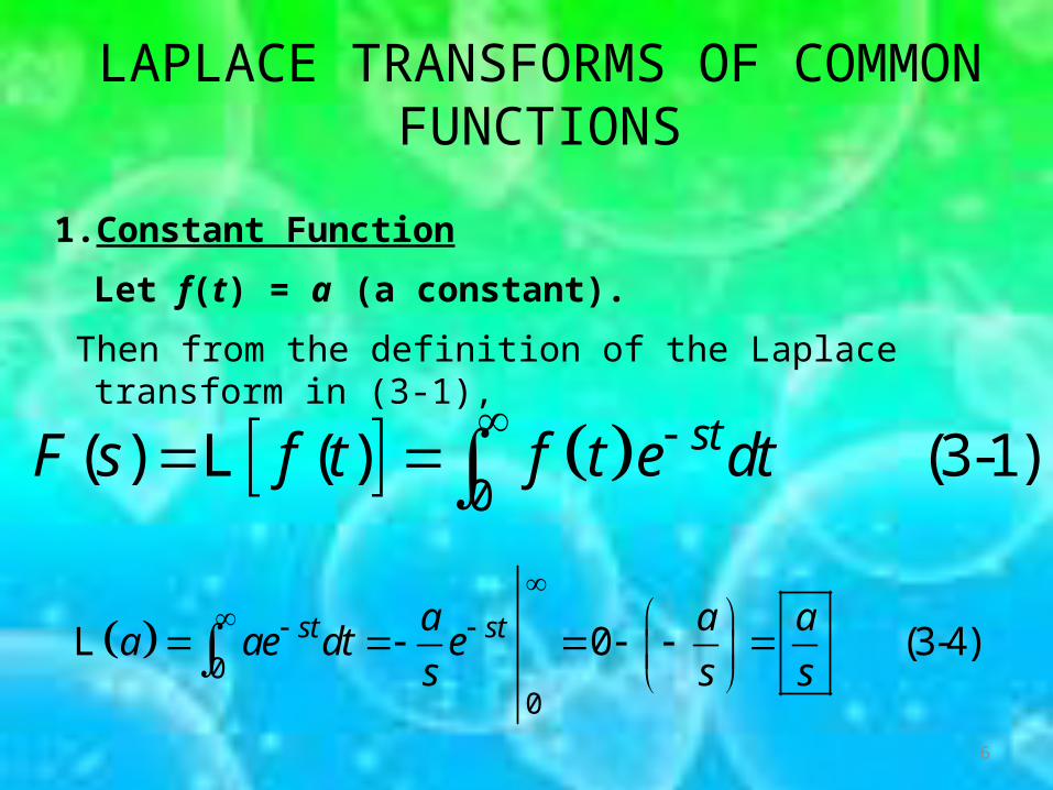
LAPLACE TRANSFORMS OF COMMON FUNCTIONS
1. Constant Function
Let f(t) = a (a constant).
Then from the definition of the Laplace transform in (3-1),
0
0
0 (3-4)st sta a aa ae dt e
s s s
L
0
( ) ( ) (3-1)stF s f t f t e dt L
7
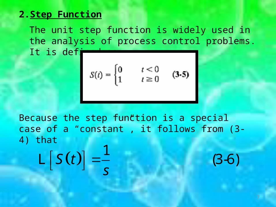
2. Step Function
The unit step function is widely used in the analysis of process control problems. It is defined as:
Because the step function is a special case of a “constant”, it follows from (3-4) that
1(3-6)S t
s L
8
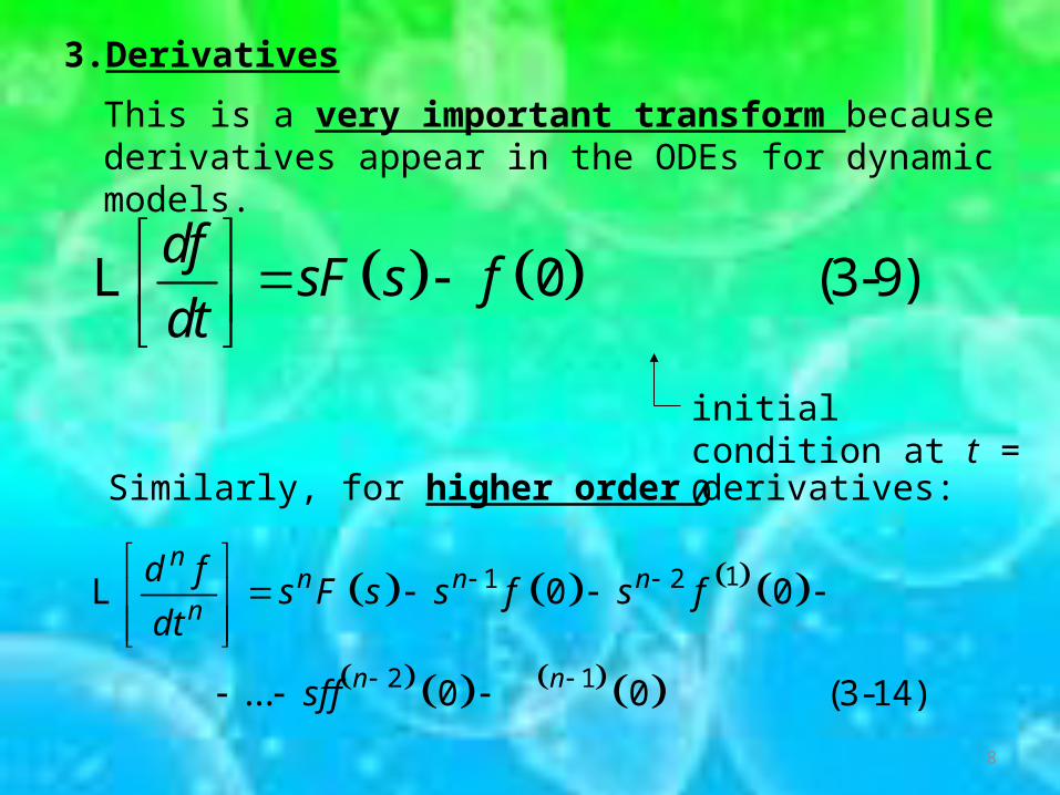
3. Derivatives
This is a very important transform because derivatives appear in the ODEs for dynamic models.
0 (3-9)df
sF s fdt
L
initial condition at t = 0
Similarly, for higher order derivatives:
11 2
2 1
0 0
... 0 0 (3-14)
nn n n
n
n n
d fs F s s f s f
dt
sf f
L
9
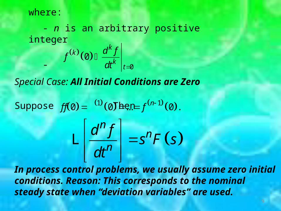
where:
- n is an arbitrary positive integer
- 0
0k
kk
t
d ff
dt
Special Case: All Initial Conditions are Zero
Suppose Then
In process control problems, we usually assume zero initial conditions. Reason: This corresponds to the nominal steady state when “deviation variables” are used.
1 10 0 ... 0 .nf f f
n
nn
d fs F s
dt
L
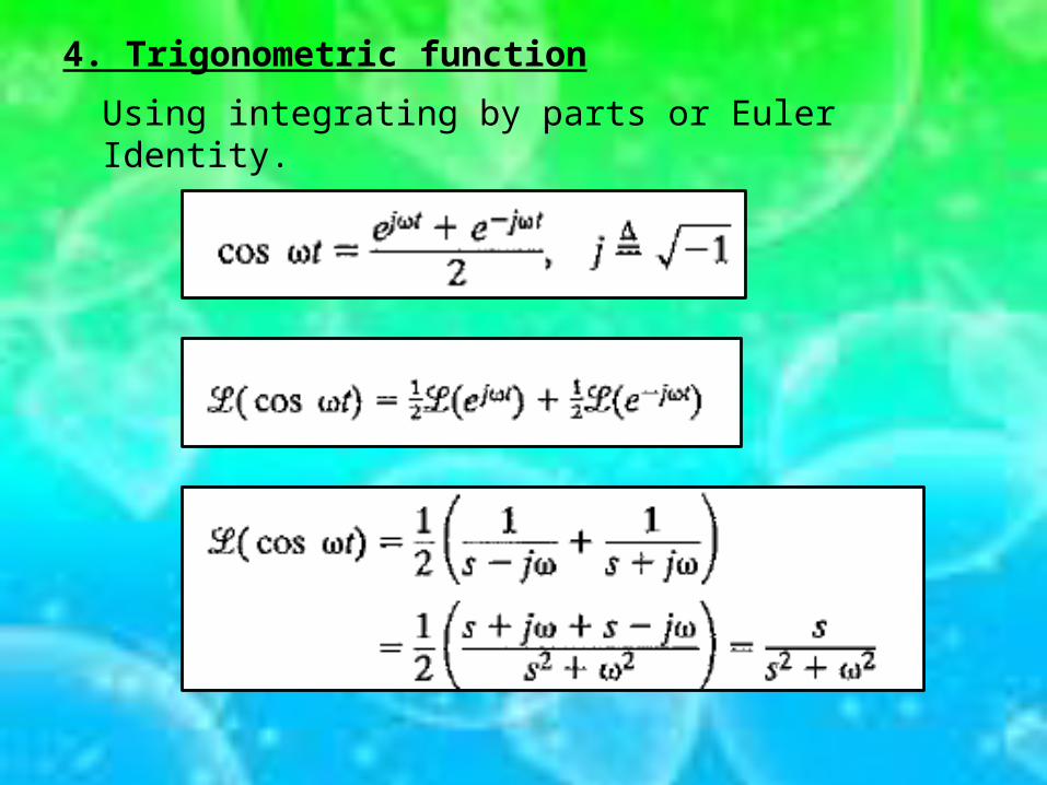
4. Trigonometric function
Using integrating by parts or Euler Identity.
11
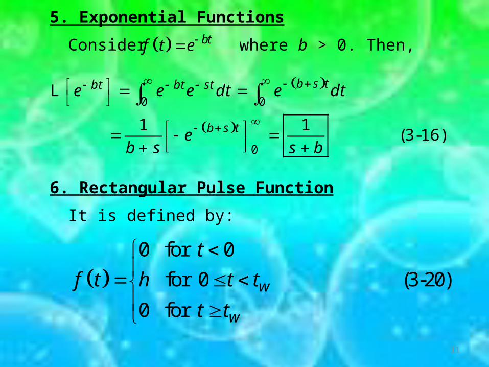
5. Exponential Functions
Consider where b > 0. Then, btf t e
0 0
0
1 1(3-16)
b s tbt bt st
b s t
e e e dt e dt
eb s s b
L
6. Rectangular Pulse Function
It is defined by:
0 for 0
for 0 (3-20)
0 forw
w
t
f t h t t
t t
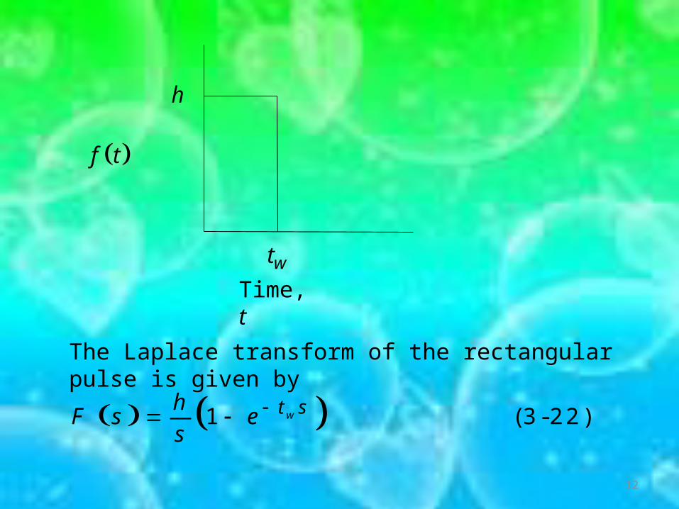
12
h
f t
wt
Time, t
The Laplace transform of the rectangular pulse is given by
1 (3-22)wt shF s e
s
13
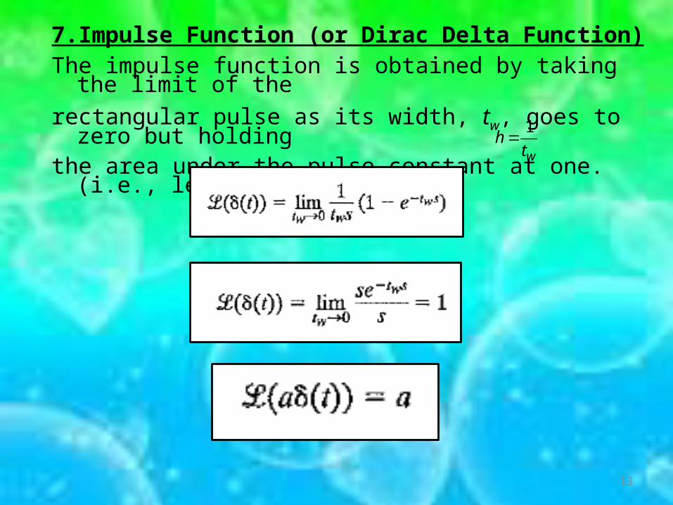
7.Impulse Function (or Dirac Delta Function)The impulse function is obtained by taking the limit of the
rectangular pulse as its width, tw, goes to zero but holdingthe area under the pulse constant at one. (i.e., let )1
w
ht
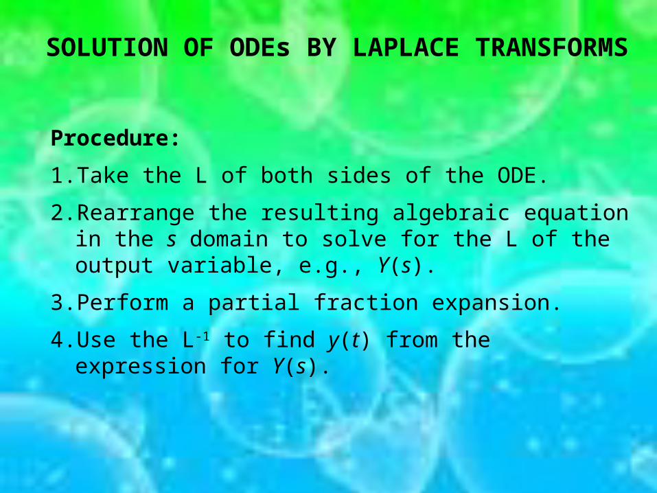
SOLUTION OF ODEs BY LAPLACE TRANSFORMS
Procedure:
1. Take the L of both sides of the ODE.
2. Rearrange the resulting algebraic equation in the s domain to solve for the L of the output variable, e.g., Y(s).
3. Perform a partial fraction expansion.
4. Use the L-1 to find y(t) from the expression for Y(s).
15
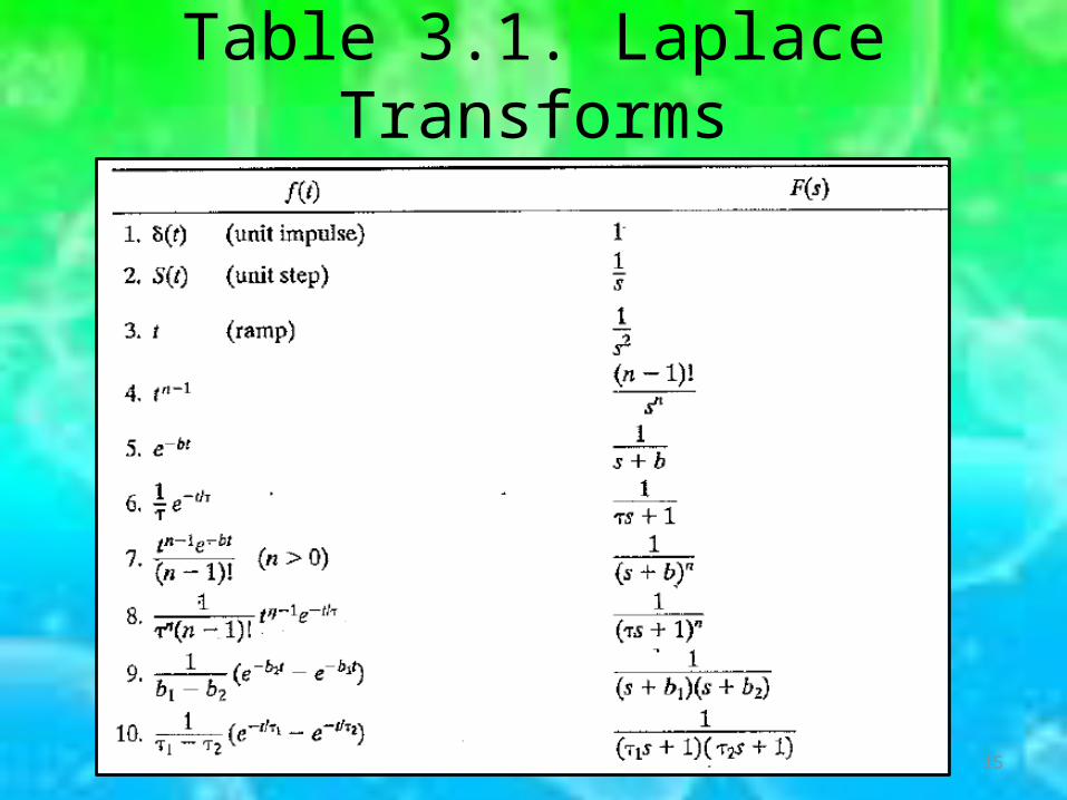
Table 3.1. Laplace Transforms
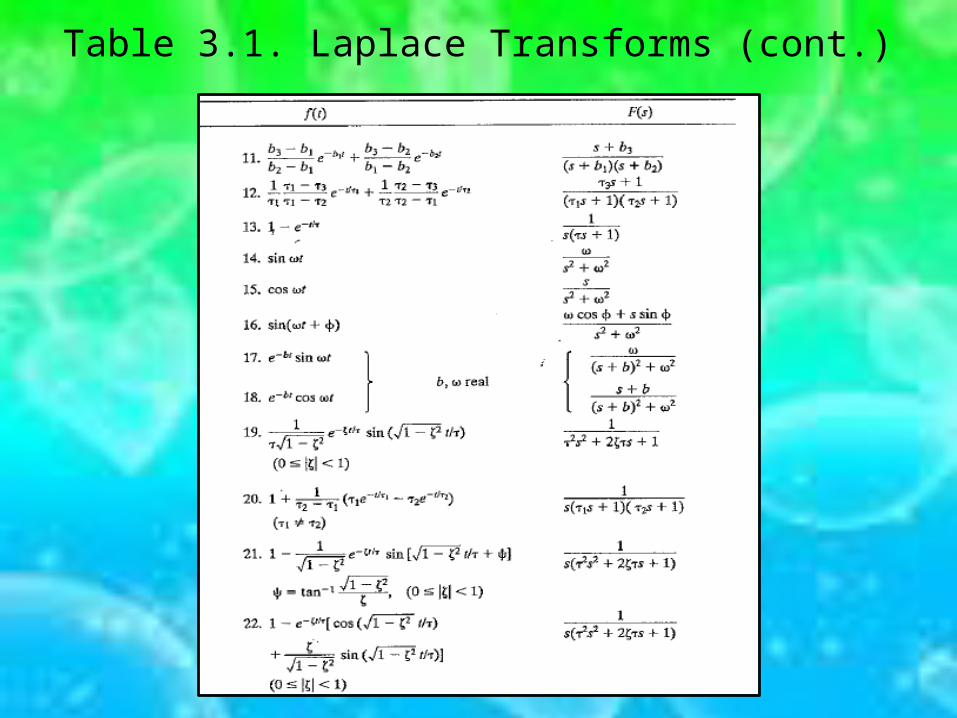
Table 3.1. Laplace Transforms (cont.)
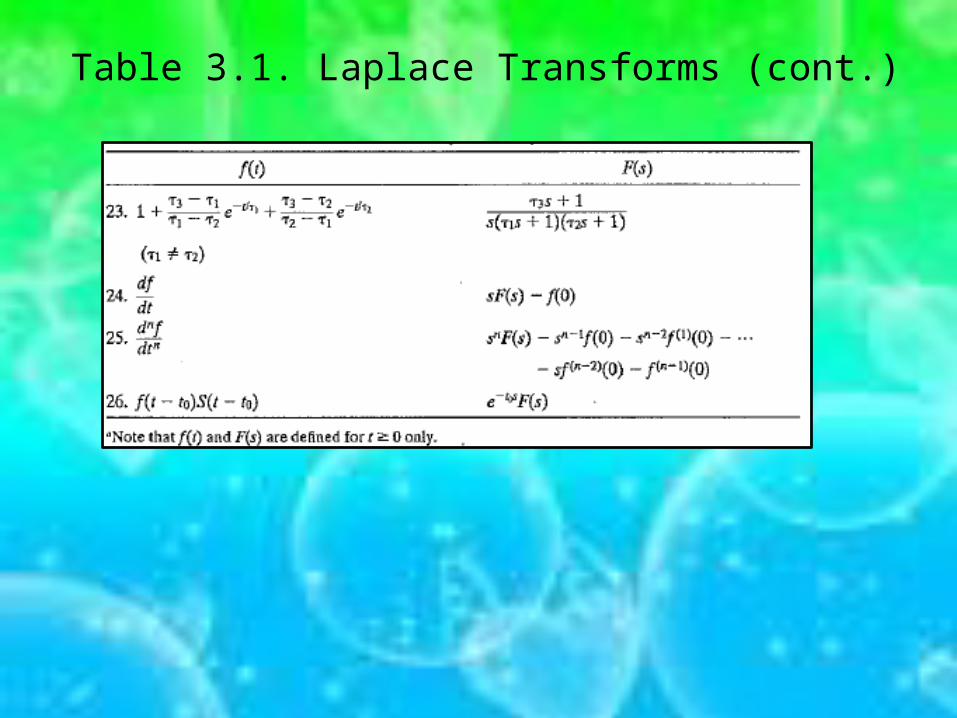
Table 3.1. Laplace Transforms (cont.)
18
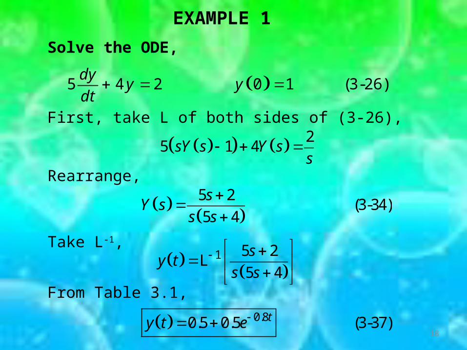
EXAMPLE 1
Solve the ODE,
5 4 2 0 1 (3-26)dy
y ydt
First, take L of both sides of (3-26),
25 1 4sY s Y s
s
Rearrange,
5 2
(3-34)5 4
sY s
s s
Take L-1,
1 5 2
5 4
sy t
s s
L
From Table 3.1,
0.80.5 0.5 (3-37)ty t e
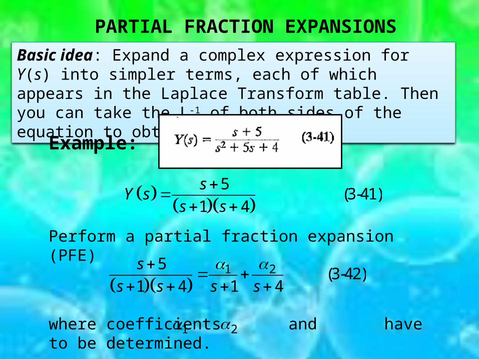
PARTIAL FRACTION EXPANSIONS
Basic idea: Expand a complex expression for Y(s) into simpler terms, each of which appears in the Laplace Transform table. Then you can take the L-1 of both sides of the equation to obtain y(t).
Example:
5
(3-41)1 4
sY s
s s
Perform a partial fraction expansion (PFE)
1 25
(3-42)1 4 1 4
s
s s s s
where coefficients and have to be determined.1 2
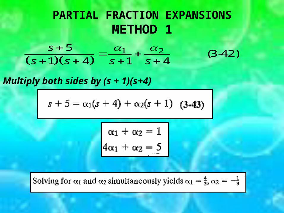
PARTIAL FRACTION EXPANSIONSMETHOD 1
1 25
(3-42)1 4 1 4
s
s s s s
Multiply both sides by (s + 1)(s+4)
1 25
(3-42)1 4 1 4
s
s s s s
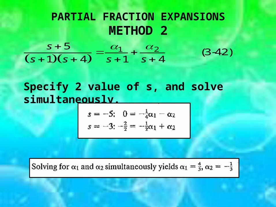
PARTIAL FRACTION EXPANSIONSMETHOD 2
Specify 2 value of s, and solve simultaneously.
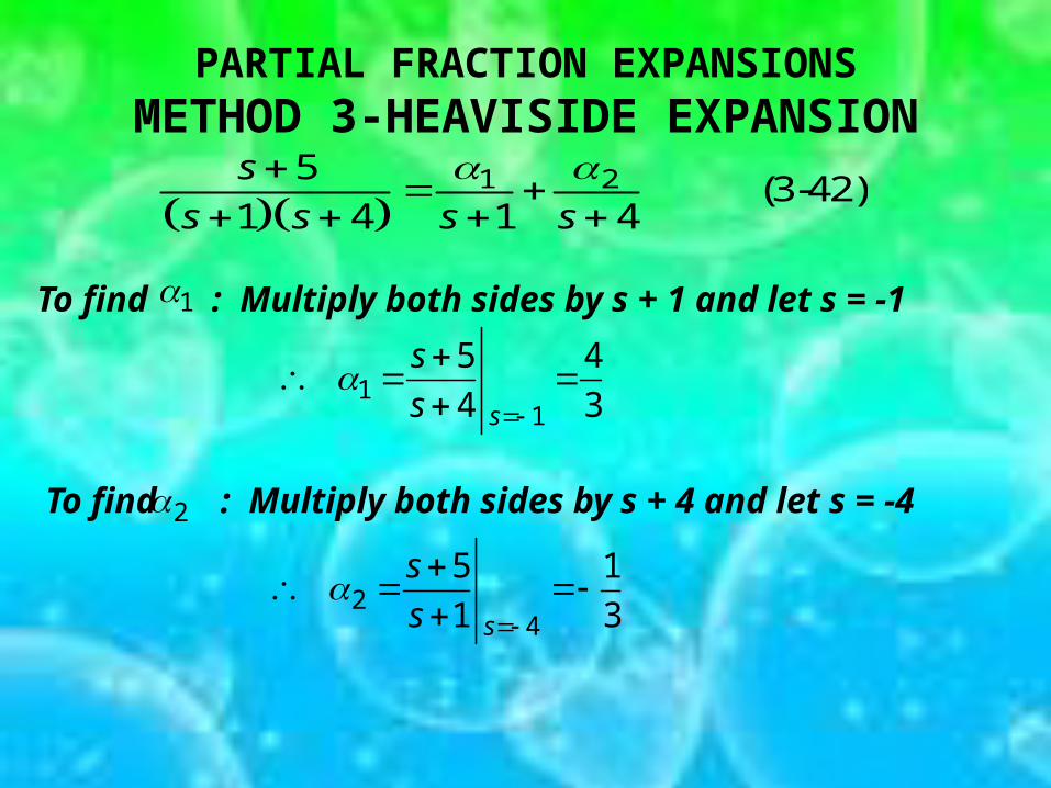
To find : Multiply both sides by s + 1 and let s = -11
11
5 4
4 3s
s
s
To find : Multiply both sides by s + 4 and let s = -42
24
5 1
1 3s
s
s
1 25
(3-42)1 4 1 4
s
s s s s
PARTIAL FRACTION EXPANSIONSMETHOD 3-HEAVISIDE EXPANSION
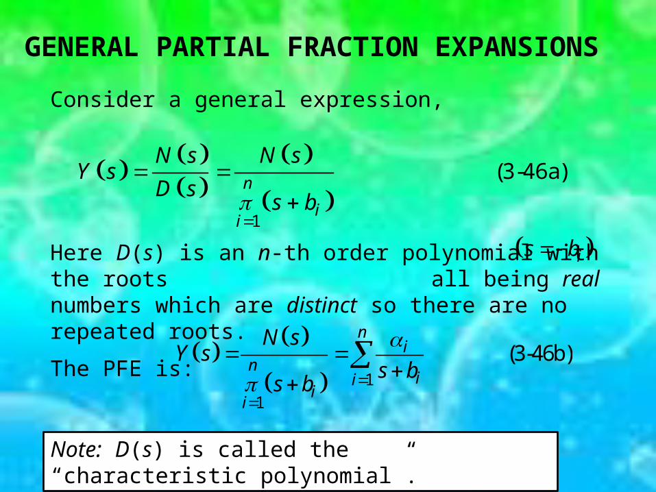
Consider a general expression,
1
(3-46a)n
ii
N s N sY s
D ss b
Here D(s) is an n-th order polynomial with the roots all being real numbers which are distinct so there are no repeated roots.
The PFE is:
GENERAL PARTIAL FRACTION EXPANSIONS
1
1
(3-46b)n
in
iii
i
N sY s
s bs b
is b
Note: D(s) is called the “characteristic polynomial”.
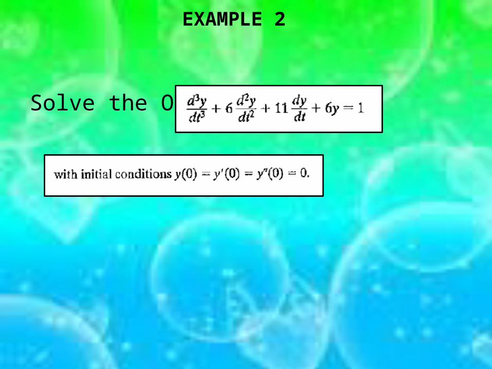
Solve the ODE;
EXAMPLE 2
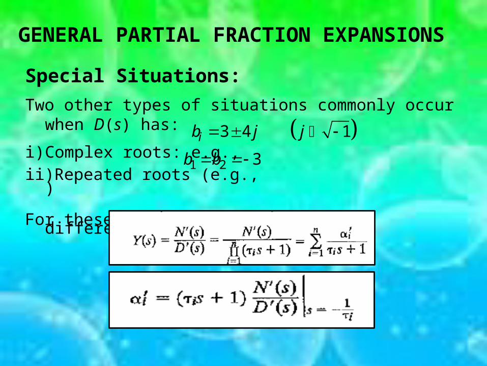
Special Situations:
Two other types of situations commonly occur when D(s) has:
i) Complex roots: e.g., ii) Repeated roots (e.g., )
For these situations, the PFE has a different form.
3 4 1ib j j
1 2 3b b
GENERAL PARTIAL FRACTION EXPANSIONS
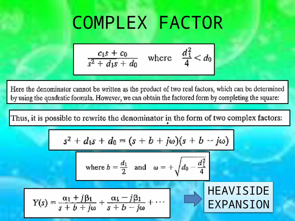
COMPLEX FACTOR
HEAVISIDE EXPANSION
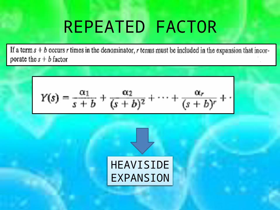
REPEATED FACTOR
HEAVISIDE EXPANSION
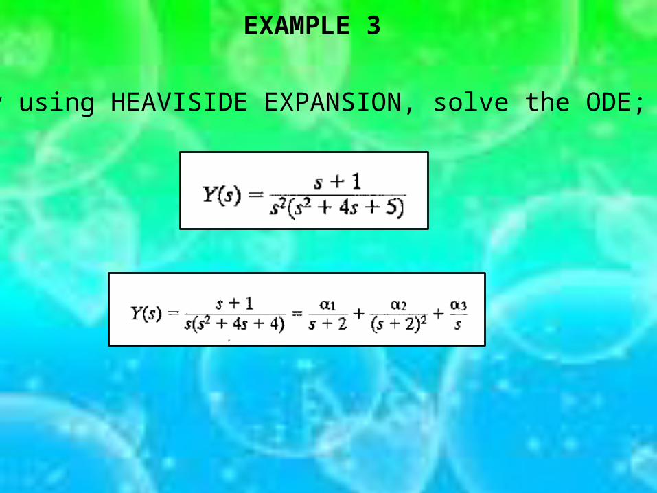
EXAMPLE 3
By using HEAVISIDE EXPANSION, solve the ODE;
29
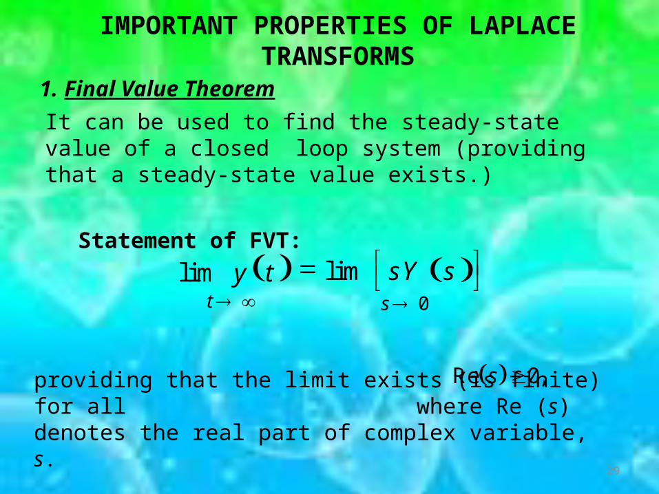
IMPORTANT PROPERTIES OF LAPLACE TRANSFORMS
1. Final Value Theorem
It can be used to find the steady-state value of a closed loop system (providing that a steady-state value exists.)
Statement of FVT:
0
limlimt s
sY sy t
providing that the limit exists (is finite) for all where Re (s) denotes the real part of complex variable, s.
Re 0,s
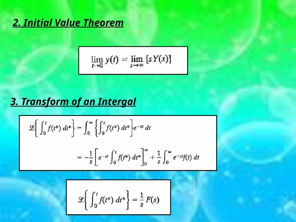
2. Initial Value Theorem
3. Transform of an Intergal
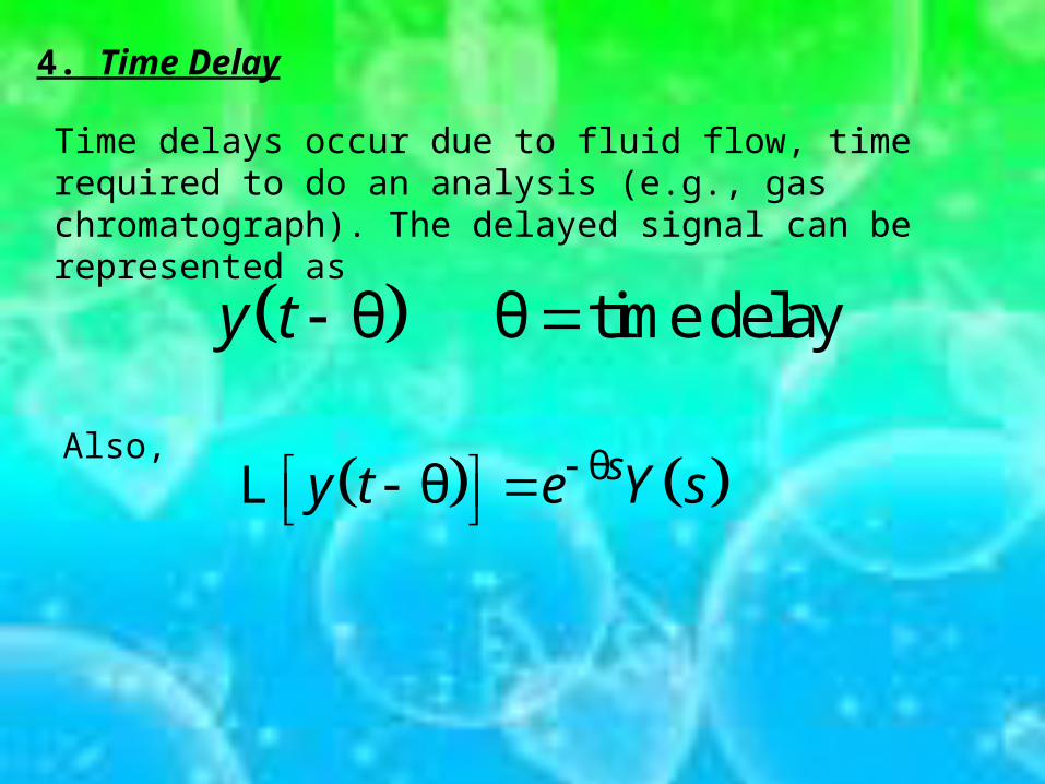
4. Time Delay
Time delays occur due to fluid flow, time required to do an analysis (e.g., gas chromatograph). The delayed signal can be represented as
θ θ time delayy t
Also,
θθ sy t e Y s L

THE ENDTHANK YOU