Large Data Bases: Advantages, Problems and Puzzles: Some naive observations from an

economist

Alan Kirman,

GREQAM Marseille

Jerusalem September 2008

Some Basic Points

• Economic data bases may be large in two ways

• Firstly they may simply contain a very large number of observations. The best examples being tick by tick data.

• Secondly as with some panel data each observation may have many dimensions.

The Advantages and Problems

• From a statistical point of view at least the high frequency data might seem to be unambiguously advantageous. However the very nature of the data has to be examined carefully and certain stylised facts emerge which are not present at lower frequency

• In the case of multidimensional data, the « curse of dimensionality » may arise.

FX: A classic example of high frequency data

• Usually Reuters indicative quotes are used for the analysis. What do they consist of?

• Banks enter bids and asks for a particular currency pair, such as the euro-dollar. They put a time stamp to indicate the exact time of posting

• These quotes are « indicative » and the banks are not legally obliged to honour them.

• For euro-dollar there are between 10 and 20 thousand updates per day.

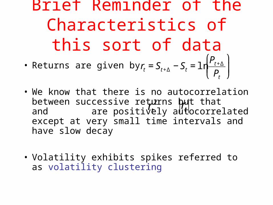
Brief Reminder of the Characteristics of this sort of data

• Returns are given by

• We know that there is no autocorrelation between successive returns but that and are positively autocorrelated except at very small time intervals and have slow decay

• Volatility exhibits spikes referred to as volatility clustering

€

rt = St +Δ − St = lnPt +Δ

Pt

⎛

⎝ ⎜

⎞

⎠ ⎟

€

rt2

€

rt

A Problem

• The idea of using such data as Brousseau (2007) points out is to track the « true value » of the exchange rate through a period.

• But all the data are not of the same « quality »• Although the quotes hold, at least briefly, between

major banks, they may not do so for other customers and they may also depend on the amounts involved.

• There may be mistakes, quotes placed as « advertising » and one with spreads so large that they encompass the spread between the best bid and ask and thus convey no information

Cleaning the Data

• Brousseau and other authors propose various filtering methods, from simple to sophisticated. If the jump between two successive mid-points exceeds a certain threshold for example the observation is eliminated. ( a primitive first run)

• However, how can one judge whether the filtering is successful?

• One idea is to test against quotes which are binding such as those on EBS. But this is not a guarantee.

Some stylised facts

Microstructure Noise

• In principle, the higher the sampling frequency is, the more precise the estimates of integrated volatility become

• However, the presence of so-called market microstructure features at very high sampling frequencies may create important complications.

• Financial transactions - and hence price changes and non-zero returns- arrive discretely rather than continuously over time

• The presence of negative serial correlation of returns to successive transactions (including the so-called bid-ask bounce), and the price impact of trades.

• For a discussion see Hasbrouck (2006), O’Hara (1998), and Campbell et al. (1997, Ch. 3)

Microstructure Noise

• Why should we treat this as « noise » rather than integrate it into our models?

• One argument is that it overemphasises volatility. In other words sampling too frequently gives a spuriously high value.

• On the other hand, Hansen and Lunde (2006) assert that empirically market microstructure noise is negatively correlated with the returns, and hence biases the estimated volatility downward. However, this empirical stylized fact, based on their analysis of high-frequency stock returns, does not seem to carry over to the FX market

Microstructure Noise• « For example, if an organized stock exchange has designated

market makers and specialists, and if these participants are slow in adjusting prices in response to shocks (possibly because the exchangeís rules explicitly prohibit them from adjusting prices by larger amounts all at once), it may be the case that realized volatility could drop if it is computed at those sampling frequencies for which this behavior is thought to be relevant.

• In any case, it is widely recognized that market microstructure issues can contaminate estimates of integrated volatility in important ways, especially if the data are sampled at ultra-high frequencies, as is becoming more and more common. »

Chaboud et al. (2007)

What do we claim to explain?

• Let’s look at rapidly at a standard model and see how we determine the prices.

• What we claim for this model is that it is the switching from chartist to fundamentalist behaviour that leads to

1. Fat tails2. Long memory3. Volatility clusteringWhat does high frequency data have to do with this?

Specifying Individual Behavior

• There is a finite set A of agents trading a single riskyasset.

• The demand function of the agent

€

a∈A takes the log-linear form :

€

eta p,ω( ):=cta ˆ S taω( )−logp( )+ηtaω( )

where

€

ˆ S taand

€

ηta denote the agent’s current reference

level and liquidity demand, respectively.

• The logarithmic equilibrium price St := log Pt is definedthrough the market clearing condition of zero totalexcess demand:

€

St:=1ct cta

a∈A∑ˆ S taω( )+ηt

Temporary equilibrium prices are given as a weightedaverage of individual price assessments and liquiditydemand.

Choosing Individual Assessments

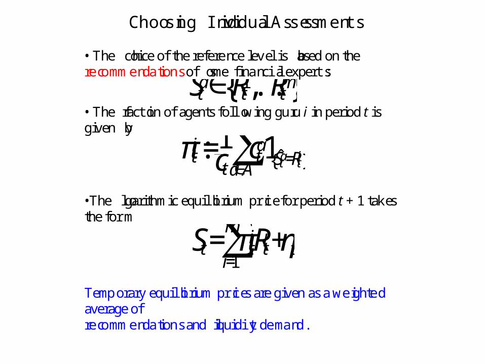
• The choice of the reference level is based on therecommendations of some financial experts:

€

ˆ S ta∈Rt1,...,Rt

m{ }• The fraction of agents following guru i in period t isgiven by

€

πti:=1

ct ctaa∈A∑1ˆ S ta=Rti{ }

•The logarithmic equilibrium price for period t + 1 takesthe form

€

St= πti

i=1

m∑Rti+ηt

Temporary equilibrium prices are given as a weightedaverage ofrecommendations and liquidity demand.

The Gurus’ Recommendations

• The recommendation of guru

€

i∈1,...,m{ }is based ona subjective assessment Fi of some fundamental valueand a price trend:

€

Rti:=St−1+αi Fi−St−1[ ]+βi St−1−St−2[ ]

• The dynamics of stock prices is governed by therecursive relation

€

St=FSt−1,St−2,τt( )=1−απt( )+βπt( )[ ]St−1−βπt( )St−2+γπt,ηt( )in the random environment

€

τt{ }= πt,ηt( ){ }• Unlike in Physics, the environment will be generatedendogenously.The dynamics of stock prices is described by a linearrecursive equation in a random environment of investorsentiment and liquidity demand.

Fundamentalists

• The recommendation of a fundamentalist conveys theidea that prices move closer to the fundamental value:

€

Rti:=St−1+αi Fi−St−1[ ], αi∈0,1( )

• If only fundamentalists are active on the market

€

St=1−απt( )[ ]St−1+γπt,ηt( ), αii=1

m∑πti

and prices behave in a mean-reverting manner because

€

αi∈0,1( )• The sequence of temporary price equilibria may beviewed as an Ornstein-Uhlenbeck process in a randomenvironment. Fundamentalists have a stabilizing effecton the dynamics of stock prices.

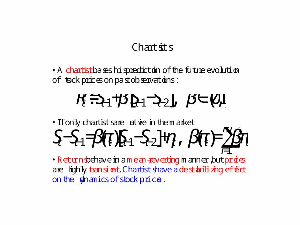
Chartists

• A chartist bases his prediction of the future evolutionof stock prices on past observations:

€

Rti:=St−1+βi St−1−St−2[ ], βi∈0,1( )

• If only chartists are active in the market

€

St−St−1=βπt( )St−1−St−2[ ]+ηt, βπt( )= βiπti

i=1

m∑• Returns behave in a mean-reverting manner, but pricesare highly transient. Chartists have a destabilizing effecton the dynamics of stock prices.

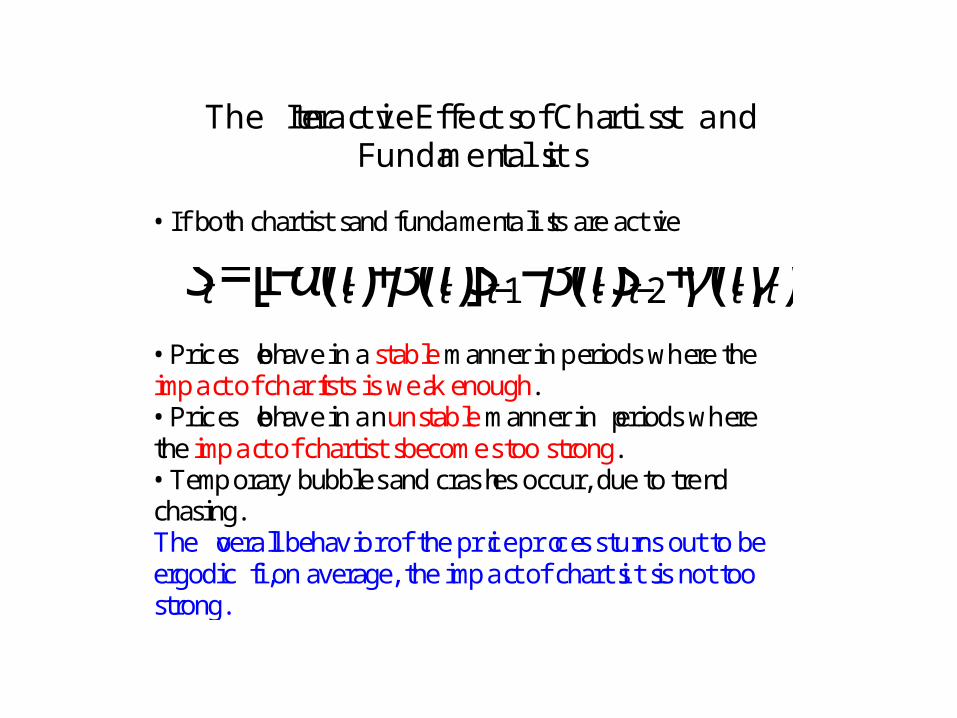
The Interactive Effects of Chartists andFundamentalists

• If both chartists and fundamentalists are active

• Prices behave in a stable manner in periods where theimpact of chartists is weak enough.• Prices behave in an unstable manner in periods wherethe impact of chartists becomes too strong.• Temporary bubbles and crashes occur, due to trendchasing.The overall behavior of the price process turns out to beergodic if, on average, the impact of chartists is not toostrong.

€

St=1−απt( )+βπt( )[ ]St−1−βπt( )St−2+γπt,γt( ),

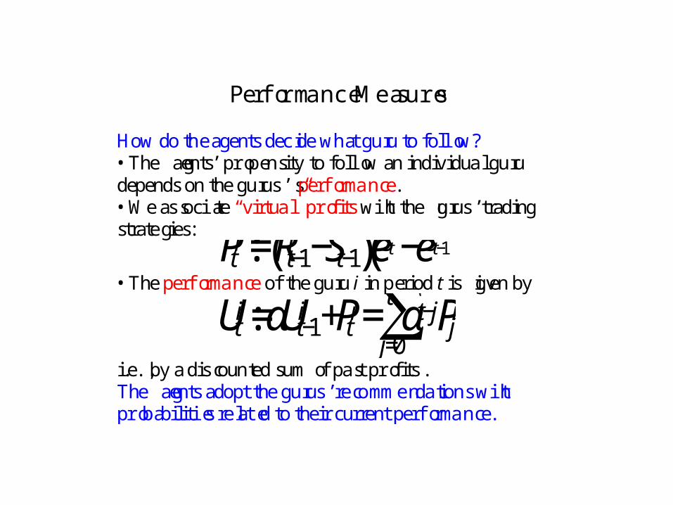
Performance Measures

How do the agents decide what guru to follow?• The agents’ propensity to follow an individual gurudepends on the gurus’s performance.• We associate “virtual” profits with the gurus’ tradingstrategies:

€

Pti:=Rt−1

i −St−1( )eSt −eSt−1( )• The performance of the guru i in period t is given by

€

Uti:=αUt−1

i +Pti= αt−j

j=0

t∑ Pji

i.e., by a discounted sum of past profits.The agents adopt the gurus’ recommendations withprobabilities related to their current performance.

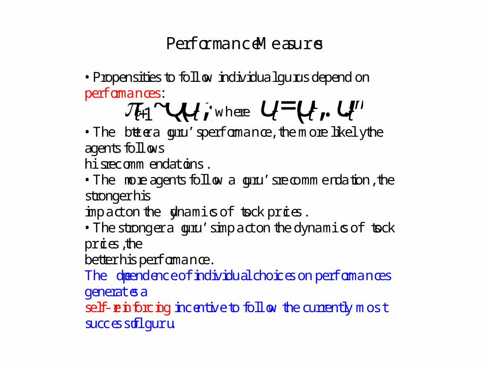
Performance Measures

• Propensities to follow individual gurus depend onperformances:

€

πt+1~QUt;⋅( ) where

€

Ut=Ut1,...,Ut

m( )• The better a guru’s performance, the more likely theagents followshis recommendations.• The more agents follow a guru’s recommendation, thestronger hisimpact on the dynamics of stock prices.• The stronger a guru’s impact on the dynamics of stockprices, thebetter his performance.The dependence of individual choices on performancesgenerates aself-reinforcing incentive to follow the currently mostsuccessful guru.

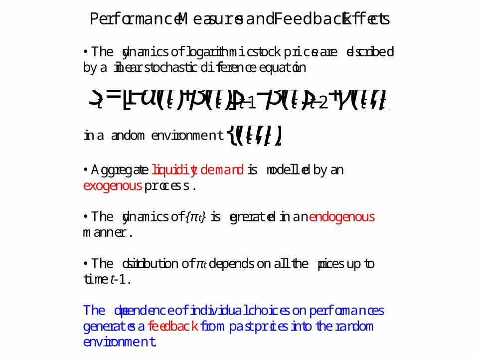
Performance Measures and Feedback Effects

• The dynamics of logarithmic stock prices are describedby a linear stochastic difference equation

€

St=1−απt( )+βπt( )[ ]St−1−βπt( )St−2+γπt,ηt( )in a random environment

€

πt,ηt( ){ }• Aggregate liquidity demand is modelled by anexogenous process.

• The dynamics of {πt} is generated in an endogenousmanner.

• The distribution of πt depends on all the prices up totime t-1.

The dependence of individual choices on performancesgenerates a feedback from past prices into the randomenvironment.

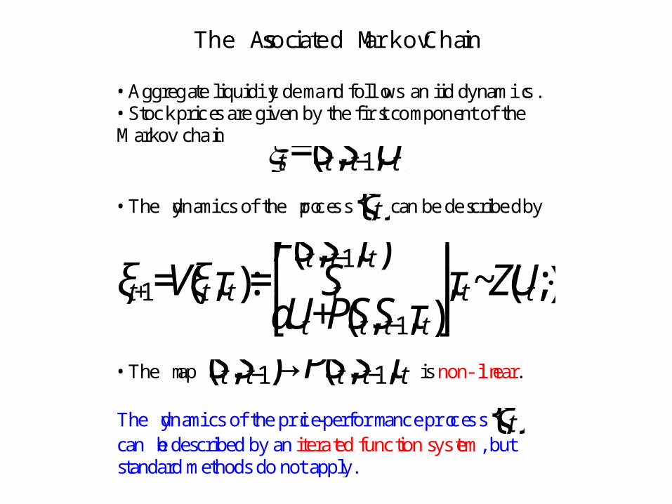
The Associated Markov Chain

• Aggregate liquidity demand follows an iid dynamics.• Stock prices are given by the first component of theMarkov chain

€

ξt=St,St−1,Ut( )• The dynamics of the process

€

ξt{ }can be described by

€

ξt+1=Vξt,τt( ):=FSt,St−1,τt( ) StαUt+PSt,St−1,τt( )

⎡

⎣ ⎢ ⎢ ⎢

⎤

⎦ ⎥ ⎥ ⎥

,τt~ZUt;⋅( ).

• The map

€

St,St−1( )→PSt,St−1,τt( ) is non-linear.

The dynamics of the price-performance process

€

ξt{ }can be described by an iterated function system, butstandard methods do not apply.

Stopping the process from exploding

• Bound the probability that an individual can become a chartist

• If we do not do this the process may simply explode

• We do not put arbitrary limits on the prices that can be attained however

Nice Story! But…

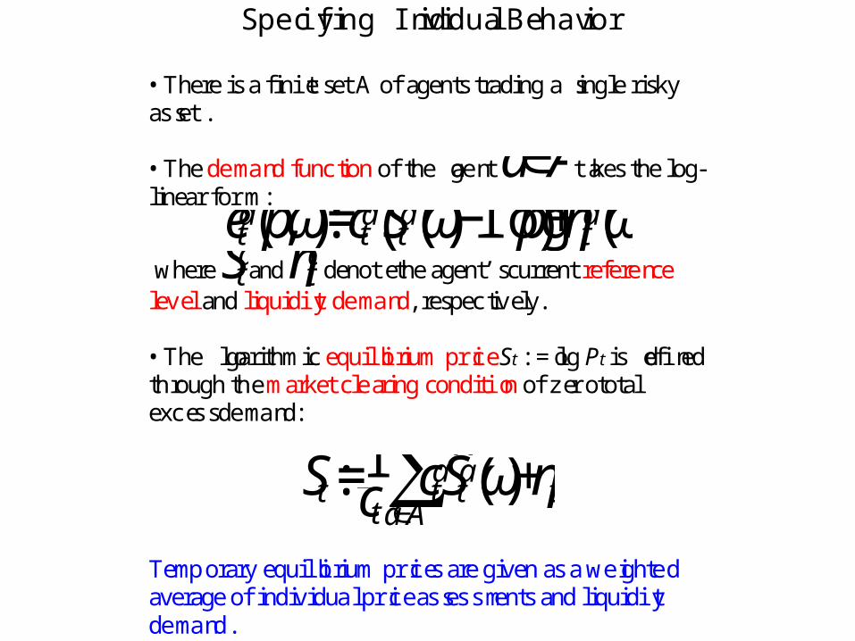
Specifying Individual Behavior

• There is a finite set A of agents trading a single riskyasset.

• The demand function of the agent

€

a∈A takes the log-linear form :

€

eta p,ω( ):=cta ˆ S taω( )−logp( )+ηtaω( )

where

€

ˆ S taand

€

ηta denote the agent’s current reference

level and liquidity demand, respectively.

• The logarithmic equilibrium price St := log Pt is definedthrough the market clearing condition of zero totalexcess demand:

€

St:=1ct cta

a∈A∑ˆ S taω( )+ηt

Temporary equilibrium prices are given as a weightedaverage of individual price assessments and liquiditydemand.

The Real Problem

• We have a market clearing equilibrium but this is not the way these markets function

• They function on the basis of an order book and that is what we should model.

• Each price in very high frequency data corresponds to an individual transaction

• The mechanics of the order book will influence the structure of the time series

• How often do our agents revise their prices?• They infer information from the actions of others

revealed by the transactions

QuickTime™ and aTIFF (Uncompressed) decompressor

are needed to see this picture.

How to solve this?

• This is the subject of a project with Ulrich Horst• We will model an arrival process for orders and

the distribution from which these orders are drawn will be determined by the movements of prices

• In this way we model directly what is too often referred to as « microstructure noise » and remove one of the problems with using high frequency data.

A Challenge

« In deep and liquid markets, market microstructure noise should pose less of a concern for volatility estimation. It should be possible to sample returns on such assets more frequently than returns on individual stocks, before estimates of integrated volatility encounter significant bias caused by the market microstructure features.. It is possible to sample the FX data as often as once every 15 to 20 seconds without the standard estimator of integrated volatility showing discernible effects stemming rom market microstructure noise. This interval is shorter than the sampling intervals of several minutes, usually five or more minutes, often recommended in the empirical literature

This shorter sampling interval and associated larger sample size affords a considerable gain in estimation precision. In very deep and liquid markets, microstructure-induced frictions may be much less of an issue for volatility estimation than was previously thought. »

Chaboud et al. (2007)

Our job is to explain why this is so!

The Curse of Dimensionality

The colorful phrase the ‘curse of dimensionality’ was apparently coined by Richard Belmanin [3], in connection with the difficulty of optimization by exhaustive enumeration onproduct spaces. Bellman reminded us that, if we consider a cartesian grid of spacing 1/10on the unit cube in 10 dimensions, we have 1010 points; if the cube in 20 dimensions wasconsidered, we would have of course 1020 points. His interpretation: if our goal is to optimizea function over a continuous product domain of a few dozen variables by exhaustivelysearching a discrete search space defined by a crude discretization, we could easily be facedwith the problem of making tens of trillions of evaluations of the function. Bellman arguedthat this curse precluded, under almost any computational scheme then foreseeable, theuse of exhaustive enumeration strategies, and argued in favor of his method of dynamicprogramming.

Why does this matter?

• We collect more and more data on individuals and, in particular, on consumers and the unemployed

• If we have D observations on N individuals the relationship between D and N is important if we wish to estimate some functional relation between the variables

• There is now a whole battery of approaches for reducing the dimensionality of the problem and these represent a major challenge for econometrics

A blessing?

• Mathematicians assert that such high dimensionality leads to a « concentration of measure »

• Someone here can no doubt explain how this might help economists!