large eddy simulation for incompressible flows
DESCRIPTION
Large Eddy Simulation for Incompressible FlowsTRANSCRIPT

7/21/2019 Large Eddy Simulation for Incompressible Flows
http://slidepdf.com/reader/full/large-eddy-simulation-for-incompressible-flows 1/573
Scientific Computation
Editorial Board
J.-J. Chattot, Davis, CA, USAP. Colella, Berkeley, CA, USAWeinan E, Princeton, NJ, USAR. Glowinski, Houston, TX, USAM. Holt, Berkeley, CA, USAY. Hussaini, Tallahassee, FL, USAP. Joly, Le Chesnay, FranceH. B. Keller, Pasadena, CA, USA
D. I. Meiron, Pasadena, CA, USAO. Pironneau, Paris, FranceA. Quarteroni, Lausanne, SwitzerlandJ. Rappaz, Lausanne, SwitzerlandR. Rosner, Chicago, IL, USA.J. H. Seinfeld, Pasadena, CA, USAA. Szepessy, Stockholm, SwedenM. F. Wheeler, Austin, TX, USA

7/21/2019 Large Eddy Simulation for Incompressible Flows
http://slidepdf.com/reader/full/large-eddy-simulation-for-incompressible-flows 2/573
Pierre Sagaut
Large Eddy Simulationfor Incompressible Flows
An Introduction
Third EditionWith a Foreword by Massimo Germano
With 99 Figures and 15 Tables
1 3

7/21/2019 Large Eddy Simulation for Incompressible Flows
http://slidepdf.com/reader/full/large-eddy-simulation-for-incompressible-flows 3/573
Prof. Dr. Pierre SagautLMM-UPMC/CNRSBoite 162, 4 place Jussieu75252 Paris Cedex 05, France
Title of the original French edition:Introduction à la simulation des grandes échelles pour les écoulements de fluide incompressible, Mathématique & Applications.© Springer Berlin Heidelberg 1998
Library of Congress Control Number: 2005930493
ISSN 1434-8322ISBN-10 3-540-26344-6 Third Edition Springer Berlin Heidelberg New YorkISBN-13 978-3-540-26344-9 Third Edition Springer Berlin Heidelberg New YorkISBN 3-540-67841-7 Second Edition Springer-Verlag Berlin Heidelberg New York
This work is subject to copyright. All rights are reserved, whether the whole or part of the material is concerned,specifically the rights of translation, reprinting, reuse of illustrations, recitation, broadcasting, reproduction onmicrofilm or in any other way, and storage in data banks. Duplication of this publication or parts thereof is permittedonly under the provisions of the German Copyright Law of September 9, 1965, in its current version, and permissionfor use must always be obtained from Springer. Violations are liable for prosecution under the German CopyrightLaw.
Springer is a part of Springer Science+Business Mediaspringeronline.com
© Springer-Verlag Berlin Heidelberg 2001, 2002, 2006Printed in Germany
The use of general descriptive names, registered names, trademarks, etc. in this publication does not imply, even in
the absence of a specific statement, that such names are exempt from the relevant protective laws and regulations andtherefore free for general use.
Typesetting: Data conversion by LE-TEX Jelonek, Schmidt & Vöckler GbR, Leipzig, Germany Cover design: design & production GmbH, Heidelberg
Printed on acid-free paper 55/3141/YL 5 4 3 2 1 0

7/21/2019 Large Eddy Simulation for Incompressible Flows
http://slidepdf.com/reader/full/large-eddy-simulation-for-incompressible-flows 4/573
Foreword to the Third Edition
It is with a sense of great satisfaction that I write these lines introducing thethird edition of Pierre Sagaut’s account of the field of Large Eddy Simulation
for Incompressible Flows. Large Eddy Simulation has evolved into a powerfultool of central importance in the study of turbulence, and this meticulouslyassembled and significantly enlarged description of the many aspects of LESwill be a most welcome addition to the bookshelves of scientists and engineersin fluid mechanics, LES practitioners, and students of turbulence in general.
Hydrodynamic turbulence continues to be a fundamental challenge forscientists striving to understand fluid motions in fields as diverse as oceanog-raphy, acoustics, meteorology and astrophysics. The challenge also has socio-economic attributes as engineers aim at predicting flows to control their fea-
tures, and to improve thermo-fluid equipment design. Drag reduction in ex-ternal aerodynamics or convective heat transfer augmentation are well-knownexamples. The fundamental challenges posed by turbulence to scientists andengineers have not, in essence, changed since the appearance of the secondedition of this book, a mere two years ago. What has evolved significantlyis the field of Large Eddy Simulation (LES), including methods developedto address the closure problem associated with LES (also called the problemof subgrid-scale modeling), numerical techniques for particular applications,and more explicit accounts of the interplay between numerical techniques and
subgrid modeling.The original hope for LES was that simple closures would be appropri-
ate, such as mixing length models with a single, universally applicable modelparameter. Kolmogorov’s phenomenological theory of turbulence in fact sup-ports this hope but only if the length-scale associated with the numericalresolution of LES falls well within the ideal inertial range of turbulence, inflows at very high Reynolds numbers. Typical applications of LES most of-ten violate this requirement and the resolution length-scale is often close tosome externally imposed scale of physical relevance, leading to loss of uni-
versality and the need for more advanced, and often much more complex,closure models. Fortunately, the LES modeler disposes of large amount of raw materials from which to assemble improved models. During LES, the re-solved motions present rich multi-scale fields and dynamics including highlynon-trivial nonlinear interactions which can be interrogated to learn about

7/21/2019 Large Eddy Simulation for Incompressible Flows
http://slidepdf.com/reader/full/large-eddy-simulation-for-incompressible-flows 5/573
VI Foreword to the Third Edition
the local state of turbulence. This availability of dynamical information hasled to the formulation of a continuously growing number of different closuremodels and methodologies and associated numerical approaches, includingmany variations on several basic themes. In consequence, the literature onLES has increased significantly in recent years. Just to mention a quantitativemeasure of this trend, in 2000 the ISI science citation index listed 164 paperspublished including the keywords ”large-eddy-simulation” during that year.By 2004 this number had doubled to over 320 per year. It is clear, then, thata significantly enlarged version of Sagaut’s book, encompassing much of whathas been added to the literature since the book’s second edition, is a mostwelcome contribution to the field.
What are the main aspects in which this third edition has been enlarged
compared to the first two? Sagaut has added significantly new material ina number of areas. To begin, the introductory chapter is enriched with anoverview of the structure of the book, including an illuminating description of three fundamental errors one incurs when attempting to solve fluid mechan-ics’ infinite-dimensional, non-linear differential equations, namely projectionerror, discretization error, and in the case of turbulence and LES, the phys-ically very important resolution error. Following the chapters describing insignificant detail the relevant foundational aspects of filtering in LES, Sagauthas added a new section dealing with alternative mathematical formulations
of LES. These include statistical approaches that replace spatial filtering withconditionally averaging the unresolved motions, and alternative model equa-tions in which the Navier-Stokes equations are replaced with mathematicallybetter behaved equations such as the Leray model in which the advectionvelocity is regularized (i.e. filtered).
In the chapter dealing with functional modeling approaches, in which thesubgrid-scale stresses are expressed in terms of local functionals of the re-solved velocity gradients, a more complete account of the various versions of the dynamic model is given, as well as extended discussions of new structure-
function and multiscale models. The chapter on structural modeling, in whichthe stress tensor is reconstructed based on its definition and various directhypotheses about the small-scale velocity field is significantly enhanced: Clo-sures in which full prognostic transport equations are solved for the subgrid-scale stress tensor are reviewed in detail, and entire new subsections have beenadded dealing with filtered density function models, with one-dimensionalturbulence mapping models, and variational multi-scale models, among oth-ers. The chapter focussing on numerical techniques contains an interestingnew description of the effects of pre-filtering and of the various methods to
perform grid refinement. In the chapter on analysis and validation of LES,a new detailed account is given about methods to evaluate the subgrid-scalekinetic energy. The description of boundary and inflow conditions for LES isenhanced with new material dealing with one-dimensional-turbulence modelsnear walls as well as stochastic tools to generate and modulate random fields
7/21/2019 Large Eddy Simulation for Incompressible Flows
http://slidepdf.com/reader/full/large-eddy-simulation-for-incompressible-flows 6/573
Foreword to the Third Edition VII
for inlet turbulence specification. Chapters dealing with coupling of multires-olution, multidomain, and adaptive grid refinement techniques, as well asLES - RANS coupling, have been extended to include recent additions to theliterature. Among others, these are areas to which Sagaut and his co-workershave made significant research contributions.
The most notable additions are two entirely new chapters at the end of the book, on the prediction of scalars using LES. Both passive scalars, forwhich subgrid-scale mixing is an important issue, and active scalars, of greatimportance to geophysical flows, are treated. The geophysics literature onLES of stably and unstably stratified flows is voluminous - the field of LESin fact traces its origins to simulating atmospheric boundary layer flows inthe early 1970s. Sagaut summarizes this vast field using his classifications of
subgrid closures introduced earlier, and the result is a conceptually elegantand concise treatment, which will be of significant interest to both engineeringand geophysics practitioners of LES.
The connection to geophysical flow prediction reminds us of the impor-tance of LES and subgrid modeling from a broader viewpoint. For the field of large-scale numerical simulation of complex multiscale nonlinear systems is,today, at the center of scientific discussions with important societal and polit-ical dimensions. This is most visible in the discussions surrounding the trust-worthiness of global change models. Among others, these include boundary-
layer parameterizations that can be studied by means of LES done at smallerscales. And LES of turbulence is itself a prime example of large-scale com-puting applied to prediction of a multi-scale complex system, including issuessurrounding the verification of its predictive capabilities, the testing of thecumulative accuracy of individual building blocks, and interesting issues onthe interplay of stochastic and deterministic aspects of the problem. Thusthe book - as well as its subject - Large Eddy Simulation of IncompressibleFlow, has much to offer to one of the most pressing issues of our times.
With this latest edition, Pierre Sagaut has fully solidified his position as
the preeminent cartographer of the complex and multifaceted world of LES.By mapping out the field in meticulous fashion, Sagaut’s work can indeed beregarded as a detailed and evolving atlas of the world of LES. And yet, it is nota tourist guide: as with any relatively young terrain in which the main routeshave not yet been firmly established, what is called for is unbiased, objective,and sophisticated cartography. The cartographer describes the topography,scenery, and landmarks as they appear, without attempting to preach to thetraveler which route is best. In return, the traveler is expected to bring alonga certain sophistication to interpret the maps and to discern which among the
many paths will most likely lead towards particular destinations of interest.The reader of this latest edition will thus be rewarded with a most solid, in-sightful, and up-to-date account of an important and exciting field of research.
Baltimore, January 2005 Charles Meneveau

7/21/2019 Large Eddy Simulation for Incompressible Flows
http://slidepdf.com/reader/full/large-eddy-simulation-for-incompressible-flows 7/573
Foreword to the Second Edition
It is a particular pleasure to present the second edition of the book on LargeEddy Simulation for Incompressible Flows written by Pierre Sagaut: two edi-
tions in two years means that the interest in the topic is strong and thata book on it was indeed required. Compared to the first one, this secondedition is a greatly enriched version, motivated both by the increasing theo-retical interest in Large Eddy Simulation (LES) and the increasing numbersof applications and practical issues. A typical one is the need to decreasethe computational cost, and this has motivated two entirely new chaptersdevoted to the coupling of LES with multiresolution multidomain techniquesand to the new hybrid approaches that relate the LES procedures to theclassical statistical methods based on the Reynolds Averaged Navier–Stokes
equations.Not that literature on LES is scarce. There are many article reviews and
conference proceedings on it, but the book by Sagaut is the first that orga-nizes a topic that by its peculiar nature is at the crossroads of various interestsand techniques: first of all the physics of turbulence and its different levels of description, then the computational aspects, and finally the applications thatinvolve a lot of different technical fields. All that has produced, particularlyduring the last decade, an enormous number of publications scattered overscientific journals, technical notes, and symposium acta, and to select and
classify with a systematic approach all this material is a real challenge. Also,by assuming, as the writer does, that the reader has a basic knowledge of fluid mechanics and applied mathematics, it is clear that to introduce theprocedures presently adopted in the large eddy simulation of turbulent flowsis a difficult task in itself. First of all, there is no accepted universal definitionof what LES really is. It seems that LES covers everything that lies betweenRANS, the classical statistical picture of turbulence based on the ReynoldsAveraged Navier–Stokes equations, and DNS, the Direct Numerical Simula-tions resolved in all details, but till now there has not been a general unified
theory that gradually goes from one description to the other. Moreover weshould note the different importance that the practitioners of LES attributeto the numerical and the modeling aspects. At one end the supporters of the no model way of thinking argue that the numerical scheme should andcould capture by itself the resolved scales. At the other end the theoretical

7/21/2019 Large Eddy Simulation for Incompressible Flows
http://slidepdf.com/reader/full/large-eddy-simulation-for-incompressible-flows 8/573
X Foreword to the Second Edition
modelers try to develop new universal equations for the filtered quantities.In some cases LES is regarded as a technique imposed by the present pro-visional inability of the computers to solve all the details. Others think thatLES modeling is a contribution to the understanding of turbulence and theinteractions among different ideas are often poor.
Pierre Sagaut has elaborated on this immense material with an open mindand in an exceptionally clear way. After three chapters devoted to the basicproblem of the scale separation and its application to the Navier–Stokes equa-tions, he classifies the various subgrid models presently in use as functionaland structural ones. The chapters devoted to this general review are of theutmost interest: obviously some selection has been done, but both the stu-dent and the professional engineer will find there a clear unbiased exposition.
After this first part devoted to the fundamentals a second part covers manyof the interdisciplinary problems created by the practical use of LES andits coupling with the numerical techniques. These subjects, very importantobviously from the practical point of view, are also very rich in theoreticalaspects, and one great merit of Sagaut is that he presents them always inan attractive way without reducing the exposition to a mere set of instruc-tions. The interpretation of the numerical solutions, the validation and thecomparison of LES databases, the general problem of the boundary condi-tions are mathematically, physically and numerically analyzed in great detail,
with a principal interest in the general aspects. Two entirely new chaptersare devoted to the coupling of LES with multidomain techniques, a topic inwhich Pierre Sagaut and his group have made important contributions, andto the new hybrid approaches RANS/LES, and finally in the last expandedchapter, enriched by new examples and beautiful figures, we have a review of the different applications of LES in the nuclear, aeronautical, chemical andautomotive fields.
Both for graduate students and for scientists this book is a very impor-tant reference. People involved in the large eddy simulation of turbulent flows
will find a useful introduction to the topic and a complete and systematicoverview of the many different modeling procedures. At present their numberis very high and in the last chapter the author tries to draw some conclusionsconcerning their efficiency, but probably the person who is only interestedin the basic question “What is the best model for LES? ” will remain a lit-tle disappointed. As remarked by the author, both the structural and thefunctional models have their advantages and disadvantages that make themseem complementary, and probably a mixed modeling procedure will be inthe future a good compromise. But for a textbook this is not the main point.
The fortunes and the misfortunes of a model are not so simple to predict,and its success is in many cases due to many particular reasons. The resultsare obviously the most important test, but they also have to be consideredin a textbook with a certain reserve, in the higher interest of a presentationthat tries as much as possible to be not only systematic but also rational.
7/21/2019 Large Eddy Simulation for Incompressible Flows
http://slidepdf.com/reader/full/large-eddy-simulation-for-incompressible-flows 9/573
Foreword to the Second Edition XI
To write a textbook obliges one in some way or another to make judgements,and to transmit ideas, sometimes hidden in procedures that for some rea-son or another have not till now received interest from the various groupsinvolved in LES and have not been explored in full detail.
Pierre Sagaut has succeeded exceptionally well in doing that. One reasonfor the success is that the author is curious about every detail. The final taskis obviously to provide a good and systematic introduction to the beginner,as rational as a book devoted to turbulence can be, and to provide usefulinformation for the specialist. The research has, however, its peculiarities,and this book is unambiguously written by a passionate researcher, disposedto explore every problem, to search in all models and in all proposals thegerms of new potentially useful ideas. The LES procedures that mix theoret-
ical modeling and numerical computation are often, in an inextricable way,exceptionally rich in complex problems. What about the problem of the mesh adaptation on unstructured grids for large eddy simulations? Or the prob-lem of the comparison of the LES results with reference data? Practice shows that nearly all authors make comparisons with reference data or analyze large eddy simulation data with no processing of the data .... Pierre Sagaut has thecourage to dive deep into procedures that are sometimes very difficult to ex-plore, with the enthusiasm of a genuine researcher interested in all aspectsand confident about every contribution. This book now in its second edition
seems really destined for a solid and durable success. Not that every aspectof LES is covered: the rapid progress of LES in compressible and reactingflows will shortly, we hope, motivate further additions. Other developmentswill probably justify new sections. What seems, however, more important isthat the basic style of this book is exceptionally valid and open to the futureof a young, rapidly evolving discipline. This book is not an encyclopedia andit is not simply a monograph, it provides a framework that can be used asa text of lectures or can be used as a detailed and accurate review of model-ing procedures. The references, now increased in number to nearly 500, are
given not only to extend but largely to support the material presented, andin some cases the dialogue goes beyond the original paper. As such, the bookis recommended as a fundamental work for people interested in LES: thegraduate and postgraduate students will find an immense number of stim-ulating issues, and the specialists, researchers and engineers involved in themore and more numerous fields of application of LES will find a reasoned andsystematic handbook of different procedures. Last, but not least, the appliedmathematician can finally enjoy considering the richness of challenging andattractive problems proposed as a result of the interaction among different
topics.
Torino, April 2002 Massimo Germano
7/21/2019 Large Eddy Simulation for Incompressible Flows
http://slidepdf.com/reader/full/large-eddy-simulation-for-incompressible-flows 10/573
Foreword to the First Edition
Still today, turbulence in fluids is considered as one of the most difficultproblems of modern physics. Yet we are quite far from the complexity of
microscopic molecular physics, since we only deal with Newtonian mechanicslaws applied to a continuum, in which the effect of molecular fluctuationshas been smoothed out and is represented by molecular-viscosity coefficients.Such a system has a dual behaviour of determinism in the Laplacian sense,and extreme sensitivity to initial conditions because of its very strong non-linear character. One does not know, for instance, how to predict the criticalReynolds number of transition to turbulence in a pipe, nor how to computeprecisely the drag of a car or an aircraft, even with today’s largest computers.
We know, since the meteorologist Richardson,1 numerical schemes allow-
ing us to solve in a deterministic manner the equations of motion, startingwith a given initial state and with prescribed boundary conditions. Theyare based on momentum and energy balances. However, such a resolutionrequires formidable computing power, and is only possible for low Reynoldsnumbers. These Direct-Numerical Simulations may involve calculating theinteraction of several million interacting sites. Generally, industrial, natu-ral, or experimental configurations involve Reynolds numbers that are fartoo large to allow direct simulations,2 and the only possibility then is LargeEddy Simulations, where the small-scale turbulent fluctuations are them-
selves smoothed out and modelled via eddy-viscosity and diffusivity assump-tions. The history of large eddy simulations began in the 1960s with thefamous Smagorinsky model. Smagorinsky, also a meteorologist, wanted torepresent the effects upon large synoptic quasi-two-dimensional atmosphericor oceanic motions3 of a three-dimensional subgrid turbulence cascading to-ward small scales according to mechanisms described by Richardson in 1926and formalized by the famous mathematician Kolmogorov in 1941.4 It is in-teresting to note that Smagorinsky’s model was a total failure as far as the
1 L.F. Richardson, Weather Prediction by Numerical Process , Cambridge Univer-
sity Press (1922).2 More than 1015 modes should be necessary for a supersonic-plane wing!3 Subject to vigorous inverse-energy cascades.4 L.F. Richardson, Proc. Roy. Soc. London, Ser A, 110, pp. 709–737 (1926); A. Kol-
mogorov, Dokl. Akad. Nauk SSSR, 30, pp. 301–305 (1941).

7/21/2019 Large Eddy Simulation for Incompressible Flows
http://slidepdf.com/reader/full/large-eddy-simulation-for-incompressible-flows 11/573
XIV Foreword to the First Edition
atmosphere and oceans are concerned, because it dissipates the large-scalemotions too much. It was an immense success, though, with users interestedin industrial-flow applications, which shows that the outcomes of researchare as unpredictable as turbulence itself! A little later, in the 1970s, the the-oretical physicist Kraichnan5 developed the important concept of spectraleddy viscosity, which allows us to go beyond the separation-scale assumptioninherent in the typical eddy-viscosity concept of Smagorinsky. From thenon, the history of large eddy simulations developed, first in the wake of twoschools: Stanford–Torino, where a dynamic version of Smagorinsky’s modelwas developed; and Grenoble, which followed Kraichnan’s footsteps. Thenresearchers, including industrial researchers, all around the world became in-fatuated with these techniques, being aware of the limits of classical modeling
methods based on the averaged equations of motion (Reynolds equations).It is a complete account of this young but very rich discipline, the large
eddy simulation of turbulence, which is proposed to us by the young ON-ERA researcher Pierre Sagaut, in a book whose reading brings pleasure andinterest. Large-Eddy Simulation for Incompressible Flows - An Introduction very wisely limits itself to the case of incompressible fluids, which is a suit-able starting point if one wants to avoid multiplying difficulties. Let us pointout, however, that compressible flows quite often exhibit near-incompressibleproperties in boundary layers, once the variation of the molecular viscosity
with the temperature has been taken into account, as predicted by Morkovinin his famous hypothesis.6 Pierre Sagaut shows an impressive culture, de-scribing exhaustively all the subgrid-modeling methods for simulating thelarge scales of turbulence, without hesitating to give the mathematical de-tails needed for a proper understanding of the subject.
After a general introduction, he presents and discusses the various filtersused, in cases of statistically homogeneous and inhomogeneous turbulence,and their applications to Navier–Stokes equations. He very aptly describesthe representation of various tensors in Fourier space, Germano-type relations
obtained by double filtering, and the consequences of Galilean invariance of the equations. He then goes into the various ways of modeling isotropic tur-bulence. This is done first in Fourier space, with the essential wave-vectortriad idea, and a discussion of the transfer-localness concept. An excellentreview of spectral-viscosity models is provided, with developments going be-yond the original papers. Then he goes to physical space, with a discussion of the structure-function models and the dynamic procedures (Eulerian and La-grangian, with energy equations and so forth). The study is then generalizedto the anisotropic case. Finally, functional approaches based on Taylor se-
ries expansions are discussed, along with non-linear models, homogenizationtechniques, and simple and dynamic mixed models.
5 He worked as a postdoctoral student with Einstein at Princeton.6 M.V. Morkovin, in Mecanique de la Turbulence , A. Favre et al. (eds.), CNRS,
pp. 367–380 (1962).

7/21/2019 Large Eddy Simulation for Incompressible Flows
http://slidepdf.com/reader/full/large-eddy-simulation-for-incompressible-flows 12/573
Foreword to the First Edition XV
Pierre Sagaut also discusses the importance of numerical errors, and pro-poses a very interesting review of the different wall models in the boundarylayers. The last chapter gives a few examples of applications carried out atONERA and a few other French laboratories. These examples are well chosenin order of increasing complexity: isotropic turbulence, with the non-linearcondensation of vorticity into the “worms” vortices discovered by Siggia;7
planar Poiseuille flow with ejection of “hairpin” vortices above low-speedstreaks; the round jet and its alternate pairing of vortex rings; and, finally,the backward-facing step, the unavoidable test case of computational fluiddynamics. Also on the menu: beautiful visualizations of separation behinda wing at high incidence, with the shedding of superb longitudinal vortices.Completing the work are two appendices on the statistical and spectral anal-
ysis of turbulence, as well as isotropic and anisotropic EDQNM modeling.A bold explorer, Pierre Sagaut had the daring to plunge into the jungle
of multiple modern techniques of large-scale simulation of turbulence. Hecame back from his trek with an extremely complete synthesis of all themodels, giving us a very complete handbook that novices can use to start off on this enthralling adventure, while specialists can discover models differentfrom those they use every day. Large-Eddy Simulation for Incompressible Flows - An Introduction is a thrilling work in a somewhat austere wrapping.I very warmly recommend it to the broad public of postgraduate students,
researchers, and engineers interested in fluid mechanics and its applicationsin numerous fields such as aerodynamics, combustion, energetics, and theenvironment.
Grenoble, March 2000 Marcel Lesieur
7 E.D. Siggia, J. Fluid Mech., 107, pp. 375–406 (1981).
7/21/2019 Large Eddy Simulation for Incompressible Flows
http://slidepdf.com/reader/full/large-eddy-simulation-for-incompressible-flows 13/573
Preface to the Third Edition
Working on the manuscript of the third edition of this book was a veryexciting task, since a lot of new developments have been published since the
second edition was printed.The large-eddy simulation (LES) technique is now recognized as a power-
ful tool and real applications in several engineering fields are more and morefrequently found. This increasing demand for efficient LES tools also sustainsgrowing theoretical research on many aspects of LES, some of which are in-cluded in this book. Among them, it is worth noting the mathematical mod-els of LES (the convolution filter being only one possiblity), the definition of boundary conditions, the coupling with numerical errors, and, of course, theproblem of defining adequate subgrid models. All these issues are discussed
in more detail in this new edition. Some good news is that other monographs,which are good complements to the present book, are now available, showingthat LES is a topic with a fastly growing audience. The reader interested inmathematics-oriented discussions will find many details in the monoghaphsby Volker John (Large-Eddy Simulation of Turbulent Incompressible Flows ,Springer) and Berselli, Illiescu and Layton (Mathematics of Large-Eddy Sim-ulation of Turbulent Flows , Springer), while people looking for a subsequentdescription of numerical methods for LES and direct numerical simulationwill enjoy the book by Bernard Geurts (Elements of Direct and Large-Eddy
Simulation , Edwards). More monographs devoted to particular features of LES (implicit LES appraoches, mathematical backgrounds, etc.) are to comein the near future.
My purpose while writing this third edition was still to provide the readerwith an up-to-date review of existing methods, approaches and models forLES of incompressible flows. All chapters of the previous edition have beenupdated, with the hope that this nearly exhaustive review will help interestedreaders avoid rediscovering old things. I would like to apologize in advance forcertainly forgetting some developments. Two entirely new chapters have been
added. The first one deals with mathematical models for LES. Here, I believethat the interesting point is that the filtering approach is nothing but a modelfor the true LES problem, and other models have been developed that seemto be at least as promising as this very popular one. The second new chapteris dedicated to the scalar equation, with both passive scalar and active scalar

7/21/2019 Large Eddy Simulation for Incompressible Flows
http://slidepdf.com/reader/full/large-eddy-simulation-for-incompressible-flows 14/573
XVIII Preface to the Third Edition
(stable/unstable stratification effects) cases being discussed. This extensionillustrates the way the usual LES can be extended and how new physicalmechanisms can be dealt with, but also inspires new problems.
Paris, November 2004 Pierre Sagaut

7/21/2019 Large Eddy Simulation for Incompressible Flows
http://slidepdf.com/reader/full/large-eddy-simulation-for-incompressible-flows 15/573
Preface to the Second Edition
The astonishingly rapid development of the Large-Eddy Simulation techniqueduring the last two or three years, both from the theoretical and applied
points of view, have rendered the first edition of this book lacunary in someways. Three to four years ago, when I was working on the manuscript of thefirst edition, coupling between LES and multiresolution/multilevel techniqueswas just an emerging idea. Nowadays, several applications of this approachhave been succesfully developed and applied to several flow configurations.Another example of interest from this exponentially growing field is the de-velopment of hybrid RANS/LES approaches, which have been derived undermany different forms. Because these topics are promising and seem to bepossible ways of enhancing the applicability of LES, I felt that they should
be incorporated in a general presentation of LES.Recent developments in LES theory also deal with older topics which have
been intensely revisited by reseachers: a unified theory for deconvolution andscale similarity ways of modeling have now been established; the “no model”approach, popularized as the MILES approach, is now based on a deepertheoretical analysis; a lot of attention has been paid to the problem of thedefinition of boundary conditions for LES; filtering has been extended toNavier–Stokes equations in general coordinates and to Eulerian time–domainfiltering.
Another important fact is that LES is now used as an engineering toolfor several types of applications, mainly dealing with massively separatedflows in complex configurations. The growing need for unsteady, accuratesimulations, more and more associated with multidisciplinary applicationssuch as aeroacoustics, is a very powerful driver for LES, and it is certain thatthis technique is of great promise.
For all these reasons, I accepted the opportunity to revise and to augmentthis book when Springer offered it me. I would also like to emphasize the fruit-ful interactions between “traditional” LES researchers and mathematicians
that have very recently been developed, yielding, for example, a better under-standing of the problem of boundary conditions. Mathematical foundationsfor LES are under development, and will not be presented in this book, be-cause I did not want to include specialized functional analysis discussions inthe present framework.

7/21/2019 Large Eddy Simulation for Incompressible Flows
http://slidepdf.com/reader/full/large-eddy-simulation-for-incompressible-flows 16/573
XX Preface to the Second Edition
I am indebted to an increasing number of people, but I would like toexpress special thanks to all my colleagues at ONERA who worked with meon LES: Drs. E. Garnier, E. Labourasse, I. Mary, P. Quemere and M. Terracol.All the people who provided me with material dealing with their researchare also warmly acknowledged. I also would like to thank all the readersof the first edition of this book who very kindly provided me with theirremarks, comments and suggestions. Mrs. J. Ryan is once again gratefullyacknowledged for her help in writing the English version.
Paris, April 2002 Pierre Sagaut
7/21/2019 Large Eddy Simulation for Incompressible Flows
http://slidepdf.com/reader/full/large-eddy-simulation-for-incompressible-flows 17/573
Preface to the First Edition
While giving lectures dealing with Large-Eddy Simulation (LES) to studentsor senior scientists, I have found difficulties indicating published references
which can serve as general and complete introductions to this technique.I have tried therefore to write a textbook which can be used by students
or researchers showing theoretical and practical aspects of the Large EddySimulation technique, with the purpose of presenting the main theoreticalproblems and ways of modeling. It assumes that the reader possesses a basicknowledge of fluid mechanics and applied mathematics.
Introducing Large Eddy Simulation is not an easy task, since no unifiedand universally accepted theoretical framework exists for it. It should beremembered that the first LES computations were carried out in the early
1960s, but the first rigorous derivation of the LES governing equations ingeneral coordinates was published in 1995! Many reasons can be invoked toexplain this lack of a unified framework. Among them, the fact that LESstands at the crossroads of physical modeling and numerical analysis is a ma-
jor point, and only a few really successful interactions between physicists,mathematicians and practitioners have been registered over the past thirtyyears, each community sticking to its own language and center of interest.Each of these three communities, though producing very interesting work,has not yet provided a complete theoretical framework for LES by its own
means. I have tried to gather these different contributions in this book, inan understandable form for readers having a basic background in appliedmathematics.
Another difficulty is the very large number of existing physical models,referred to as subgrid models. Most of them are only used by their creators,and appear in a very small number of publications. I made the choice topresent a very large number of models, in order to give the reader a goodoverview of the ways explored. The distinction between functional and struc-tural models is made in this book, in order to provide a general classification;
this was necessary to produce an integrated presentation.In order to provide a useful synthesis of forty years of LES development,I had to make several choices. Firstly, the subject is restricted to incom-pressible flows, as the theoretical background for compressible flow is lessevolved. Secondly, it was necessary to make a unified presentation of a large
7/21/2019 Large Eddy Simulation for Incompressible Flows
http://slidepdf.com/reader/full/large-eddy-simulation-for-incompressible-flows 18/573
XXII Preface to the First Edition
number of works issued from many research groups, and very often I havehad to change the original proof and to reduce it. I hope that the authorswill not feel betrayed by the present work. Thirdly, several thousand jour-nal articles and communications dealing with LES can be found, and I hadto make a selection. I have deliberately chosen to present a large numberof theoretical approaches and physical models to give the reader the mostgeneral view of what has been done in each field. I think that the most im-portant contributions are presented in this book, but I am sure that manynew physical models and results dealing with theoretical aspects will appearin the near future.
A typical question of people who are discovering LES is “what is the bestmodel for LES?”. I have to say that I am convinced that this question cannot
be answered nowadays, because no extensive comparisons have been carriedout, and I am not even sure that the answer exists, because people do notagree on the criterion to use to define the “best” model. As a consequence,I did not try to rank the model, but gave very generally agreed conclusionson the model efficiency.
A very important point when dealing with LES is the numerical algorithmused to solve the governing equations. It has always been recognized thatnumerical errors could affect the quality of the solution, but new emphasishas been put on this subject during the last decade, and it seems that things
are just beginning. This point appeared as a real problem to me when writingthis book, because many conclusions are still controversial (e.g. the possibilityof using a second-order accurate numerical scheme or an artificial diffusion).So I chose to mention the problems and the different existing points of view,but avoided writing a part dealing entirely with numerical discretization andtime integration, discretization errors, etc. This would have required writinga companion book on numerical methods, and that was beyond the scope of the present work. Many good textbooks on that subject already exist, andthe reader should refer to them.
Another point is that the analysis of the coupling of LES with typicalnumerical techniques, which should greatly increase the range of applications,such as Arbitrary Lagrangian–Eulerian methods, Adaptive Mesh-Refinementor embedded grid techniques, is still to be developed.
I am indebted to a large number of people, but I would like to expressspecial thanks to Dr. P. Le Quere, O. Daube, who gave me the opportunity towrite my first manuscript on LES, and to Prof. J.M. Ghidaglia who offered methe possibility of publishing the first version of this book (in French). I wouldalso like to thank ONERA for helping me to write this new, augmented and
translated version of the book. Mrs. J. Ryan is gratefully acknowledged forher help in writing the English version.
Paris, September 2000 Pierre Sagaut

7/21/2019 Large Eddy Simulation for Incompressible Flows
http://slidepdf.com/reader/full/large-eddy-simulation-for-incompressible-flows 19/573
Contents
1. Introduction . . . . . . . . . . . . . . . . . . . . . . . . . . . . . . . . . . . . . . . . . . . . . . 1
1.1 Computational Fluid Dynamics . . . . . . . . . . . . . . . . . . . . . . . . . . 11.2 Levels of Approximation: General . . . . . . . . . . . . . . . . . . . . . . . . 21.3 Statement of the Scale Separation Problem . . . . . . . . . . . . . . . . 31.4 Usual Levels of Approximation . . . . . . . . . . . . . . . . . . . . . . . . . . . 51.5 Large-Eddy Simulation: from Practice to Theory.
Structure of the Book . . . . . . . . . . . . . . . . . . . . . . . . . . . . . . . . . . . 9
2. Formal Introduction to Scale Separation:Band-Pass Filtering . . . . . . . . . . . . . . . . . . . . . . . . . . . . . . . . . . . . . . . 15
2.1 Definition and Properties of the Filterin the Homogeneous Case . . . . . . . . . . . . . . . . . . . . . . . . . . . . . . . 152.1.1 Definition . . . . . . . . . . . . . . . . . . . . . . . . . . . . . . . . . . . . . . . 152.1.2 Fundamental Properties . . . . . . . . . . . . . . . . . . . . . . . . . . . 172.1.3 Characterization of Different Approximations . . . . . . . . 182.1.4 Differential Filters . . . . . . . . . . . . . . . . . . . . . . . . . . . . . . . . 202.1.5 Three Classical Filters for Large-Eddy Simulation . . . . 212.1.6 Differential Interpretation of the Filters . . . . . . . . . . . . . 26
2.2 Spatial Filtering: Extension to the Inhomogeneous Case . . . . . 31
2.2.1 General . . . . . . . . . . . . . . . . . . . . . . . . . . . . . . . . . . . . . . . . . 312.2.2 Non-uniform Filtering Over an Arbitrary Domain . . . . 322.2.3 Local Spectrum of Commutation Error . . . . . . . . . . . . . . 42
2.3 Time Filtering: a Few Properties . . . . . . . . . . . . . . . . . . . . . . . . . 43
3. Application to Navier–Stokes Equations . . . . . . . . . . . . . . . . . . 453.1 Navier–Stokes Equations . . . . . . . . . . . . . . . . . . . . . . . . . . . . . . . . 46
3.1.1 Formulation in Physical Space . . . . . . . . . . . . . . . . . . . . . 463.1.2 Formulation in General Coordinates . . . . . . . . . . . . . . . . 463.1.3 Formulation in Spectral Space . . . . . . . . . . . . . . . . . . . . . 47
3.2 Filtered Navier–Stokes Equations in Cartesian Coordinates(Homogeneous Case) . . . . . . . . . . . . . . . . . . . . . . . . . . . . . . . . . . . . 483.2.1 Formulation in Physical Space . . . . . . . . . . . . . . . . . . . . . 483.2.2 Formulation in Spectral Space . . . . . . . . . . . . . . . . . . . . . 48

7/21/2019 Large Eddy Simulation for Incompressible Flows
http://slidepdf.com/reader/full/large-eddy-simulation-for-incompressible-flows 20/573
XXIV Contents
3.3 Decomposition of the Non-linear Term.Associated Equations for the Conventional Approach . . . . . . . 493.3.1 Leonard’s Decomposition . . . . . . . . . . . . . . . . . . . . . . . . . . 493.3.2 Germano Consistent Decomposition . . . . . . . . . . . . . . . . 593.3.3 Germano Identity . . . . . . . . . . . . . . . . . . . . . . . . . . . . . . . . 613.3.4 Invariance Properties . . . . . . . . . . . . . . . . . . . . . . . . . . . . . 643.3.5 Realizability Conditions . . . . . . . . . . . . . . . . . . . . . . . . . . . 72
3.4 Extension to the Inhomogeneous Casefor the Conventional Approach . . . . . . . . . . . . . . . . . . . . . . . . . . . 743.4.1 Second-Order Commuting Filter . . . . . . . . . . . . . . . . . . . . 743.4.2 High-Order Commuting Filters . . . . . . . . . . . . . . . . . . . . . 77
3.5 Filtered Navier–Stokes Equations in General Coordinates . . . . 77
3.5.1 Basic Form of the Filtered Equations . . . . . . . . . . . . . . . 773.5.2 Simplified Form of the Equations –
Non-linear Terms Decomposition . . . . . . . . . . . . . . . . . . . 783.6 Closure Problem . . . . . . . . . . . . . . . . . . . . . . . . . . . . . . . . . . . . . . . 78
3.6.1 Statement of the Problem . . . . . . . . . . . . . . . . . . . . . . . . . 783.6.2 Postulates . . . . . . . . . . . . . . . . . . . . . . . . . . . . . . . . . . . . . . . 793.6.3 Functional and Structural Modeling . . . . . . . . . . . . . . . . 80
4. Other Mathematical Models for the Large-Eddy
Simulation Problem . . . . . . . . . . . . . . . . . . . . . . . . . . . . . . . . . . . . . . 834.1 Ensemble-Averaged Models . . . . . . . . . . . . . . . . . . . . . . . . . . . . . . 83
4.1.1 Yoshizawa’s Partial Statistical Average Model . . . . . . . . 834.1.2 McComb’s Conditional Mode Elimination Procedure . . 84
4.2 Regularized Navier–Stokes Models . . . . . . . . . . . . . . . . . . . . . . . . 854.2.1 Leray’s Model. . . . . . . . . . . . . . . . . . . . . . . . . . . . . . . . . . . . 864.2.2 Holm’s Navier–Stokes-α Model . . . . . . . . . . . . . . . . . . . . . 864.2.3 Ladyzenskaja’s Model . . . . . . . . . . . . . . . . . . . . . . . . . . . . . 89
5. Functional Modeling (Isotropic Case) . . . . . . . . . . . . . . . . . . . . . 915.1 Phenomenology of Inter-Scale Interactions . . . . . . . . . . . . . . . . . 915.1.1 Local Isotropy Assumption: Consequences . . . . . . . . . . . 925.1.2 Interactions Between Resolved and Subgrid Scales . . . . 935.1.3 A View in Physical Space . . . . . . . . . . . . . . . . . . . . . . . . . 1025.1.4 Summary . . . . . . . . . . . . . . . . . . . . . . . . . . . . . . . . . . . . . . . . 104
5.2 Basic Functional Modeling Hypothesis . . . . . . . . . . . . . . . . . . . . 1045.3 Modeling of the Forward Energy Cascade Process . . . . . . . . . . 105
5.3.1 Spectral Models . . . . . . . . . . . . . . . . . . . . . . . . . . . . . . . . . . 1055.3.2 Physical Space Models . . . . . . . . . . . . . . . . . . . . . . . . . . . . 1095.3.3 Improvement of Models in the Physical Space . . . . . . . 1335.3.4 Implicit Diffusion: the ILES Concept . . . . . . . . . . . . . . . . 161
5.4 Modeling the Backward Energy Cascade Process . . . . . . . . . . . 1715.4.1 Preliminary Remarks . . . . . . . . . . . . . . . . . . . . . . . . . . . . . 171

7/21/2019 Large Eddy Simulation for Incompressible Flows
http://slidepdf.com/reader/full/large-eddy-simulation-for-incompressible-flows 21/573
Contents XXV
5.4.2 Deterministic Statistical Models . . . . . . . . . . . . . . . . . . . . 1725.4.3 Stochastic Models . . . . . . . . . . . . . . . . . . . . . . . . . . . . . . . . 178
6. Functional Modeling:Extension to Anisotropic Cases . . . . . . . . . . . . . . . . . . . . . . . . . . . 1876.1 Statement of the Problem . . . . . . . . . . . . . . . . . . . . . . . . . . . . . . . 1876.2 Application of Anisotropic Filter to Isotropic Flow . . . . . . . . . . 187
6.2.1 Scalar Models . . . . . . . . . . . . . . . . . . . . . . . . . . . . . . . . . . . 1886.2.2 Batten’s Mixed Space-Time Scalar Estimator . . . . . . . . 1916.2.3 Tensorial Models . . . . . . . . . . . . . . . . . . . . . . . . . . . . . . . . . 191
6.3 Application of an Isotropic Filter to a Shear Flow . . . . . . . . . . 1936.3.1 Phenomenology of Inter-Scale Interactions . . . . . . . . . . . 193
6.3.2 Anisotropic Models: Scalar Subgrid Viscosities . . . . . . . 1986.3.3 Anisotropic Models: Tensorial Subgrid Viscosities . . . . . 202
6.4 Remarks on Flows Submitted to Strong Rotation Effects . . . . 208
7. Structural Modeling . . . . . . . . . . . . . . . . . . . . . . . . . . . . . . . . . . . . . . 2097.1 Introduction and Motivations . . . . . . . . . . . . . . . . . . . . . . . . . . . . 2097.2 Formal Series Expansions . . . . . . . . . . . . . . . . . . . . . . . . . . . . . . . . 210
7.2.1 Models Based on Approximate Deconvolution . . . . . . . . 2107.2.2 Non-linear Models . . . . . . . . . . . . . . . . . . . . . . . . . . . . . . . . 223
7.2.3 Homogenization-Technique-Based Models . . . . . . . . . . . . 2287.3 Scale Similarity Hypotheses and Models Using Them . . . . . . . . 2317.3.1 Scale Similarity Hypotheses . . . . . . . . . . . . . . . . . . . . . . . . 2317.3.2 Scale Similarity Models . . . . . . . . . . . . . . . . . . . . . . . . . . . 2327.3.3 A Bridge Between Scale Similarity and Approximate
Deconvolution Models. Generalized Similarity Models . 2367.4 Mixed Modeling . . . . . . . . . . . . . . . . . . . . . . . . . . . . . . . . . . . . . . . . 237
7.4.1 Motivations . . . . . . . . . . . . . . . . . . . . . . . . . . . . . . . . . . . . . . 2377.4.2 Examples of Mixed Models . . . . . . . . . . . . . . . . . . . . . . . . 239
7.5 Differential Subgrid Stress Models . . . . . . . . . . . . . . . . . . . . . . . . 2437.5.1 Deardorff Model . . . . . . . . . . . . . . . . . . . . . . . . . . . . . . . . . . 2437.5.2 Fureby Differential Subgrid Stress Model . . . . . . . . . . . . 2447.5.3 Velocity-Filtered-Density-Function-Based Subgrid
Stress Models . . . . . . . . . . . . . . . . . . . . . . . . . . . . . . . . . . . . 2457.5.4 Link with the Subgrid Viscosity Models . . . . . . . . . . . . . 248
7.6 Stretched-Vortex Subgrid Stress Models . . . . . . . . . . . . . . . . . . . 2497.6.1 General . . . . . . . . . . . . . . . . . . . . . . . . . . . . . . . . . . . . . . . . . 2497.6.2 S3/S2 Alignment Model . . . . . . . . . . . . . . . . . . . . . . . . . . . 2507.6.3 S3/ω Alignment Model . . . . . . . . . . . . . . . . . . . . . . . . . . . . 2507.6.4 Kinematic Model . . . . . . . . . . . . . . . . . . . . . . . . . . . . . . . . . 250
7.7 Explicit Evaluation of Subgrid Scales . . . . . . . . . . . . . . . . . . . . . 2517.7.1 Fractal Interpolation Procedure . . . . . . . . . . . . . . . . . . . . 2537.7.2 Chaotic Map Model . . . . . . . . . . . . . . . . . . . . . . . . . . . . . . 254

7/21/2019 Large Eddy Simulation for Incompressible Flows
http://slidepdf.com/reader/full/large-eddy-simulation-for-incompressible-flows 22/573
XXVI Contents
7.7.3 Kerstein’s ODT-Based Method . . . . . . . . . . . . . . . . . . . . . 2577.7.4 Kinematic-Simulation-Based Reconstruction . . . . . . . . . 2597.7.5 Velocity Filtered Density Function Approach . . . . . . . . . 2607.7.6 Subgrid Scale Estimation Procedure . . . . . . . . . . . . . . . . 2617.7.7 Multi-level Simulations . . . . . . . . . . . . . . . . . . . . . . . . . . . . 263
7.8 Direct Identification of Subgrid Terms . . . . . . . . . . . . . . . . . . . . . 2727.8.1 Linear-Stochastic-Estimation-Based Model . . . . . . . . . . 2747.8.2 Neural-Network-Based Model . . . . . . . . . . . . . . . . . . . . . . 275
7.9 Implicit Structural Models . . . . . . . . . . . . . . . . . . . . . . . . . . . . . . . 2757.9.1 Local Average Method . . . . . . . . . . . . . . . . . . . . . . . . . . . . 2767.9.2 Scale Residual Model . . . . . . . . . . . . . . . . . . . . . . . . . . . . . 278
8. Numerical Solution: Interpretation and Problems . . . . . . . . . 2818.1 Dynamic Interpretation of the Large-Eddy Simulation . . . . . . . 281
8.1.1 Static and Dynamic Interpretations: Effective Filter . . 2818.1.2 Theoretical Analysis of the Turbulence
Generated by Large-Eddy Simulation . . . . . . . . . . . . . . . 2838.2 Ties Between the Filter and Computational Grid.
Pre-filtering . . . . . . . . . . . . . . . . . . . . . . . . . . . . . . . . . . . . . . . . . . . . 2888.3 Numerical Errors and Subgrid Terms . . . . . . . . . . . . . . . . . . . . . 290
8.3.1 Ghosal’s General Analysis . . . . . . . . . . . . . . . . . . . . . . . . . 290
8.3.2 Pre-filtering Effect . . . . . . . . . . . . . . . . . . . . . . . . . . . . . . . . 2948.3.3 Conclusions . . . . . . . . . . . . . . . . . . . . . . . . . . . . . . . . . . . . . . 2978.3.4 Remarks on the Use of Artificial Dissipations . . . . . . . . 2998.3.5 Remarks Concerning the Time Integration Method . . . 303
9. Analysis and Validation of Large-Eddy Simulation Data . . 3059.1 Statement of the Problem . . . . . . . . . . . . . . . . . . . . . . . . . . . . . . . 305
9.1.1 Type of Information Containedin a Large-Eddy Simulation . . . . . . . . . . . . . . . . . . . . . . . . 305
9.1.2 Validation Methods . . . . . . . . . . . . . . . . . . . . . . . . . . . . . . . 3069.1.3 Statistical Equivalency Classes of Realizations . . . . . . . 3079.1.4 Ideal LES and Optimal LES . . . . . . . . . . . . . . . . . . . . . . . 3109.1.5 Mathematical Analysis of Sensitivities
and Uncertainties in Large-Eddy Simulation . . . . . . . . . 3119.2 Correction Techniques . . . . . . . . . . . . . . . . . . . . . . . . . . . . . . . . . . 313
9.2.1 Filtering the Reference Data . . . . . . . . . . . . . . . . . . . . . . . 3139.2.2 Evaluation of Subgrid-Scale Contribution . . . . . . . . . . . . 3149.2.3 Evaluation of Subgrid-Scale Kinetic Energy . . . . . . . . . . 315
9.3 Practical Experience . . . . . . . . . . . . . . . . . . . . . . . . . . . . . . . . . . . . 318
10. Boundary Conditions . . . . . . . . . . . . . . . . . . . . . . . . . . . . . . . . . . . . . 32310.1 General Problem . . . . . . . . . . . . . . . . . . . . . . . . . . . . . . . . . . . . . . . 323
10.1.1 Mathematical Aspects . . . . . . . . . . . . . . . . . . . . . . . . . . . . 32310.1.2 Physical Aspects . . . . . . . . . . . . . . . . . . . . . . . . . . . . . . . . . 324

7/21/2019 Large Eddy Simulation for Incompressible Flows
http://slidepdf.com/reader/full/large-eddy-simulation-for-incompressible-flows 23/573
Contents XXVII
10.2 Solid Walls . . . . . . . . . . . . . . . . . . . . . . . . . . . . . . . . . . . . . . . . . . . . 32610.2.1 Statement of the Problem . . . . . . . . . . . . . . . . . . . . . . . . . 32610.2.2 A Few Wall Models . . . . . . . . . . . . . . . . . . . . . . . . . . . . . . . 33210.2.3 Wall Models: Achievements and Problems . . . . . . . . . . . 351
10.3 Case of the Inflow Conditions . . . . . . . . . . . . . . . . . . . . . . . . . . . . 35410.3.1 Required Conditions . . . . . . . . . . . . . . . . . . . . . . . . . . . . . . 35410.3.2 Inflow Condition Generation Techniques . . . . . . . . . . . . . 354
11. Coupling Large-Eddy Simulationwith Multiresolution/Multidomain Techniques . . . . . . . . . . . . 36911.1 Statement of the Problem . . . . . . . . . . . . . . . . . . . . . . . . . . . . . . . 36911.2 Methods with Full Overlap . . . . . . . . . . . . . . . . . . . . . . . . . . . . . . 371
11.2.1 One-Way Coupling Algorithm . . . . . . . . . . . . . . . . . . . . . . 37211.2.2 Two-Way Coupling Algorithm . . . . . . . . . . . . . . . . . . . . . 37211.2.3 FAS-like Multilevel Method . . . . . . . . . . . . . . . . . . . . . . . . 37311.2.4 Kravchenko et al. Method . . . . . . . . . . . . . . . . . . . . . . . . . 374
11.3 Methods Without Full Overlap . . . . . . . . . . . . . . . . . . . . . . . . . . . 37611.4 Coupling Large-Eddy Simulation with Adaptive
Mesh Refinement . . . . . . . . . . . . . . . . . . . . . . . . . . . . . . . . . . . . . . . 37711.4.1 Statement of the Problem . . . . . . . . . . . . . . . . . . . . . . . . . 37711.4.2 Error Estimation . . . . . . . . . . . . . . . . . . . . . . . . . . . . . . . . . 378
12. Hybrid RANS/LES Approaches . . . . . . . . . . . . . . . . . . . . . . . . . . 38312.1 Motivations and Presentation . . . . . . . . . . . . . . . . . . . . . . . . . . . . 38312.2 Zonal Decomposition. . . . . . . . . . . . . . . . . . . . . . . . . . . . . . . . . . . . 384
12.2.1 Statement of the Problem . . . . . . . . . . . . . . . . . . . . . . . . . 38412.2.2 Sharp Transition . . . . . . . . . . . . . . . . . . . . . . . . . . . . . . . . . 38512.2.3 Smooth Transition . . . . . . . . . . . . . . . . . . . . . . . . . . . . . . . . 38712.2.4 Zonal RANS/LES Approach as Wall Model . . . . . . . . . . 388
12.3 Nonlinear Disturbance Equations . . . . . . . . . . . . . . . . . . . . . . . . . 390
12.4 Universal Modeling . . . . . . . . . . . . . . . . . . . . . . . . . . . . . . . . . . . . . 39112.4.1 Germano’s Hybrid Model . . . . . . . . . . . . . . . . . . . . . . . . . . 39212.4.2 Speziale’s Rescaling Method and Related Approaches . 39312.4.3 Baurle’s Blending Strategy . . . . . . . . . . . . . . . . . . . . . . . . 39412.4.4 Arunajatesan’s Modified Two-Equation Model . . . . . . . 39612.4.5 Bush–Mani Limiters . . . . . . . . . . . . . . . . . . . . . . . . . . . . . . 39712.4.6 Magagnato’s Two-Equation Model. . . . . . . . . . . . . . . . . . 398
12.5 Toward a Theoretical Status for HybridRANS/LES Approaches . . . . . . . . . . . . . . . . . . . . . . . . . . . . . . . . . 399
13. Implementation . . . . . . . . . . . . . . . . . . . . . . . . . . . . . . . . . . . . . . . . . . . 40113.1 Filter Identification. Computing the Cutoff Length . . . . . . . . . 40113.2 Explicit Discrete Filters . . . . . . . . . . . . . . . . . . . . . . . . . . . . . . . . . 404
13.2.1 Uniform One-Dimensional Grid Case . . . . . . . . . . . . . . . . 40413.2.2 Extension to the Multi-Dimensional Case . . . . . . . . . . . . 407

7/21/2019 Large Eddy Simulation for Incompressible Flows
http://slidepdf.com/reader/full/large-eddy-simulation-for-incompressible-flows 24/573
XXVIII Contents
13.2.3 Extension to the General Case. Convolution Filters . . . 40713.2.4 High-Order Elliptic Filters . . . . . . . . . . . . . . . . . . . . . . . . . 408
13.3 Implementation of the Structure Function Models . . . . . . . . . . 408
14. Examples of Applications . . . . . . . . . . . . . . . . . . . . . . . . . . . . . . . . . 41114.1 Homogeneous Turbulence . . . . . . . . . . . . . . . . . . . . . . . . . . . . . . . . 411
14.1.1 Isotropic Homogeneous Turbulence . . . . . . . . . . . . . . . . . 41114.1.2 Anisotropic Homogeneous Turbulence . . . . . . . . . . . . . . . 412
14.2 Flows Possessing a Direction of Inhomogeneity . . . . . . . . . . . . . 41414.2.1 Time-Evolving Plane Channel . . . . . . . . . . . . . . . . . . . . . . 41414.2.2 Other Flows . . . . . . . . . . . . . . . . . . . . . . . . . . . . . . . . . . . . . 418
14.3 Flows Having at Most One Direction of Homogeneity . . . . . . . 419
14.3.1 Round Jet . . . . . . . . . . . . . . . . . . . . . . . . . . . . . . . . . . . . . . . 41914.3.2 Backward Facing Step . . . . . . . . . . . . . . . . . . . . . . . . . . . . 42614.3.3 Square-Section Cylinder . . . . . . . . . . . . . . . . . . . . . . . . . . . 43014.3.4 Other Examples . . . . . . . . . . . . . . . . . . . . . . . . . . . . . . . . . . 431
14.4 Industrial Applications . . . . . . . . . . . . . . . . . . . . . . . . . . . . . . . . . . 43214.4.1 Large-Eddy Simulation for Nuclear Power Plants . . . . . 43214.4.2 Flow in a Mixed-Flow Pump . . . . . . . . . . . . . . . . . . . . . . . 43514.4.3 Flow Around a Landing Gear Configuration . . . . . . . . . 43714.4.4 Flow Around a Full-Scale Car . . . . . . . . . . . . . . . . . . . . . . 437
14.5 Lessons . . . . . . . . . . . . . . . . . . . . . . . . . . . . . . . . . . . . . . . . . . . . . . . 43914.5.1 General Lessons . . . . . . . . . . . . . . . . . . . . . . . . . . . . . . . . . . 43914.5.2 Subgrid Model Efficiency . . . . . . . . . . . . . . . . . . . . . . . . . . 44214.5.3 Wall Model Efficiency . . . . . . . . . . . . . . . . . . . . . . . . . . . . . 44414.5.4 Mesh Generation for Building Blocks Flows . . . . . . . . . . 445
15. Coupling with Passive/Active Scalar . . . . . . . . . . . . . . . . . . . . . . 44915.1 Scope of this Chapter . . . . . . . . . . . . . . . . . . . . . . . . . . . . . . . . . . . 44915.2 The Passive Scalar Case . . . . . . . . . . . . . . . . . . . . . . . . . . . . . . . . . 450
15.2.1 Physical Model . . . . . . . . . . . . . . . . . . . . . . . . . . . . . . . . . . . 45015.2.2 Dynamics of the Passive Scalar. . . . . . . . . . . . . . . . . . . . . 45315.2.3 Extensions of Functional Models . . . . . . . . . . . . . . . . . . . 46115.2.4 Extensions of Structural Models . . . . . . . . . . . . . . . . . . . . 46615.2.5 Generalized Subgrid Modeling for Arbitrary Non-linear
Functions of an Advected Scalar. . . . . . . . . . . . . . . . . . . . 46815.2.6 Models for Subgrid Scalar Variance and Scalar Subgrid
Mixing Rate . . . . . . . . . . . . . . . . . . . . . . . . . . . . . . . . . . . . . 46915.2.7 A Few Applications . . . . . . . . . . . . . . . . . . . . . . . . . . . . . . . 472
15.3 The Active Scalar Case: Stratification and Buoyancy Effects . 47215.3.1 Physical Model . . . . . . . . . . . . . . . . . . . . . . . . . . . . . . . . . . . 47215.3.2 Some Insights into the Active Scalar Dynamics . . . . . . . 47415.3.3 Extensions of Functional Models . . . . . . . . . . . . . . . . . . . 48115.3.4 Extensions of Structural Models . . . . . . . . . . . . . . . . . . . . 48715.3.5 Subgrid Kinetic Energy Estimates . . . . . . . . . . . . . . . . . . 490
7/21/2019 Large Eddy Simulation for Incompressible Flows
http://slidepdf.com/reader/full/large-eddy-simulation-for-incompressible-flows 25/573
Contents XXIX
15.3.6 More Complex Physical Models . . . . . . . . . . . . . . . . . . . . 49215.3.7 A Few Applications . . . . . . . . . . . . . . . . . . . . . . . . . . . . . . . 492
A. Statistical and Spectral Analysis of Turbulence . . . . . . . . . . . 495A.1 Turbulence Properties . . . . . . . . . . . . . . . . . . . . . . . . . . . . . . . . . . . 495A.2 Foundations of the Statistical Analysis of Turbulence . . . . . . . 495
A.2.1 Motivations . . . . . . . . . . . . . . . . . . . . . . . . . . . . . . . . . . . . . . 495A.2.2 Statistical Average: Definition and Properties . . . . . . . . 496A.2.3 Ergodicity Principle . . . . . . . . . . . . . . . . . . . . . . . . . . . . . . 496A.2.4 Decomposition of a Turbulent Field . . . . . . . . . . . . . . . . . 498A.2.5 Isotropic Homogeneous Turbulence . . . . . . . . . . . . . . . . . 499
A.3 Introduction to Spectral Analysis
of the Isotropic Turbulent Fields . . . . . . . . . . . . . . . . . . . . . . . . . 499A.3.1 Definitions . . . . . . . . . . . . . . . . . . . . . . . . . . . . . . . . . . . . . . 499A.3.2 Modal Interactions . . . . . . . . . . . . . . . . . . . . . . . . . . . . . . . 501A.3.3 Spectral Equations . . . . . . . . . . . . . . . . . . . . . . . . . . . . . . . 502
A.4 Characteristic Scales of Turbulence . . . . . . . . . . . . . . . . . . . . . . . 504A.5 Spectral Dynamics of Isotropic Homogeneous Turbulence . . . . 504
A.5.1 Energy Cascade and Local Isotropy . . . . . . . . . . . . . . . . 504A.5.2 Equilibrium Spectrum . . . . . . . . . . . . . . . . . . . . . . . . . . . . 505
B. EDQNM Modeling . . . . . . . . . . . . . . . . . . . . . . . . . . . . . . . . . . . . . . . 507B.1 Isotropic EDQNM Model . . . . . . . . . . . . . . . . . . . . . . . . . . . . . . . . 507B.2 Cambon’s Anisotropic EDQNM Model . . . . . . . . . . . . . . . . . . . . 509B.3 EDQNM Model for Isotropic Passive Scalar . . . . . . . . . . . . . . . . 511
Bibliography . . . . . . . . . . . . . . . . . . . . . . . . . . . . . . . . . . . . . . . . . . . . . . . . . . 513
Index . . . . . . . . . . . . . . . . . . . . . . . . . . . . . . . . . . . . . . . . . . . . . . . . . . . . . . . . . 553
7/21/2019 Large Eddy Simulation for Incompressible Flows
http://slidepdf.com/reader/full/large-eddy-simulation-for-incompressible-flows 26/573
1. Introduction
1.1 Computational Fluid Dynamics
Computational Fluid Dynamics (CFD) is the study of fluids in flow by numer-ical simulation, and is a field advancing by leaps and bounds. The basic ideais to use appropriate algorithms to find solutions to the equations describingthe fluid motion.
Numerical simulations are used for two types of purposes.The first is to accompany research of a fundamental kind. By describing
the basic physical mechanisms governing fluid dynamics better, numericalsimulation helps us understand, model, and later control these mechanisms.This kind of study requires that the numerical simulation produce data of
very high accuracy, which implies that the physical model chosen to representthe behavior of the fluid must be pertinent and that the algorithms used,and the way they are used by the computer system, must introduce no morethan a low level of error. The quality of the data generated by the numericalsimulation also depends on the level of resolution chosen. For the best possibleprecision, the simulation has to take into account all the space-time scalesaffecting the flow dynamics. When the range of scales is very large, as it isin turbulent flows, for example, the problem becomes a stiff one, in the sensethat the ratio between the largest and smallest scales becomes very large.
Numerical simulation is also used for another purpose: engineering anal-yses, where flow characteristics need to be predicted in equipment designphase. Here, the goal is no longer to produce data for analyzing the flowdynamics itself, but rather to predict certain of the flow characteristics or,more precisely, the values of physical parameters that depend on the flow,such as the stresses exerted on an immersed body, the production and prop-agation of acoustic waves, or the mixing of chemical species. The purposeis to reduce the cost and time needed to develop a prototype. The desiredpredictions may be either of the mean values of these parameters or their
extremes. If the former, the characteristics of the system’s normal operatingregime are determined, such as the fuel an aircraft will consume per unitof time in cruising flight. The question of study here is mainly the system’sperformance. When extreme parameter values are desired, the question israther the system’s characteristics in situations that have a little probabil-ity of ever existing, i.e. in the presence of rare or critical phenomena, such

7/21/2019 Large Eddy Simulation for Incompressible Flows
http://slidepdf.com/reader/full/large-eddy-simulation-for-incompressible-flows 27/573
2 1. Introduction
as rotating stall in aeronautical engines. Studies like this concern systemsafety at operating points far from the cruising regime for which they weredesigned.
The constraints on the quality of representation of the physical phenom-ena differ here from what is required in fundamental studies, because whatis wanted now is evidence that certain phenomena exist, rather than all thephysical mechanisms at play. In theory, then, the description does not haveto be as detailed as it does for fundamental studies. However, it goes withoutsaying that the quality of the prediction improves with the richness of thephysical model.
The various levels of approximation going into the physical model arediscussed in the following.
1.2 Levels of Approximation: General
A mathematical model for describing a physical system cannot be definedbefore we have determined the level of approximation that will be needed forobtaining the required precision on a fixed set of parameters (see [307] fora fuller discussion). This set of parameters, associated with the other variablescharacterizing the evolution of the model, contain the necessary informationfor describing the system completely.
The first decision that is made concerns the scale of reality considered.That is, physical reality can be described at several levels: in terms of par-ticle physics, atomic physics, or micro- and macroscopic descriptions of phe-nomena. This latter level is the one used by classical mechanics, especiallycontinuum mechanics, which will serve as the framework for the explanationsgiven here.
A system description at a given scale can be seen as a statistical averagingof the detailed descriptions obtained at the previous (lower) level of descrip-
tion. In fluid mechanics, which is essentially the study of systems consistingof a large number of interacting elements, the choice of a level of description,and thus a level of averaging, is fundamental. A description at the molecularlevel would call for a definition of a discrete system governed by Boltzmannequations, whereas the continuum paradigm would be called for in a macro-scopic description corresponding to a scale of representation larger than themean free path of the molecules. The system will then be governed by theNavier–Stokes equations, if the fluid is Newtonian.
After deciding on a level of reality, several other levels of approximation
have to be considered in order to obtain the desired information concerningthe evolution of the system:
– Level of space-time resolution . This is a matter of determining the time andspace scales characteristic of the system evolution. The smallest pertinent
7/21/2019 Large Eddy Simulation for Incompressible Flows
http://slidepdf.com/reader/full/large-eddy-simulation-for-incompressible-flows 28/573
1.3 Statement of the Scale Separation Problem 3
scale is taken as the resolution reference so as to capture all the dynamicmechanisms. The system spatial dimension (zero to three dimensions) hasto be determined in addition to this.
– Level of dynamic description . Here we determine the various forces ex-erted on the system components, and their relative importance. In thecontinuum mechanics framework, the most complete model is that of theNavier–Stokes equations, complemented by empirical laws for describingthe dependency of the diffusion coefficients as a function of the other vari-ables, and the state law. This can first be simplified by considering thatthe elliptic character of the flow is due only to the pressure, while the othervariables are considered to be parabolic, and we then refer to the parabolicNavier–Stokes equations. Other possible simplifications are, for example,
Stokes equations, which account only for the pressure and diffusion effects,and the Euler equations, which neglect the viscous mechanisms.
The different choices made at each of these levels make it possible to de-velop a mathematical model for describing the physical system. In all of thefollowing, we restrict ourselves to the case of a Newtonian fluid of a singlespecies, of constant volume, isothermal, and isochoric in the absence of anyexternal forces. The mathematical model consists of the unsteady Navier–Stokes equations. The numerical simulation then consists in finding solutions
of these equations using algorithms for Partial Differential Equations. Be-cause of the way computers are structured, the numerical data thus generatedis a discrete set of degrees of freedom, and of finite dimensions. We thereforeassume that the behavior of the discrete dynamical system represented bythe numerical result will approximate that of the exact, continuous solutionof the Navier–Stokes equations with adequate accuracy.
1.3 Statement of the Scale Separation Problem
Solving the unsteady Navier–Stokes equations implies that we must take intoaccount all the space-time scales of the solution if we want to have a resultof maximum quality. The discretization has to be fine enough to representall these scales numerically. That is, the simulation is discretized in steps∆x in space and ∆t in time that must be smaller, respectively, than thecharacteristic length and the characteristic time associated with the smallestdynamically active scale of the exact solution. This is equivalent to sayingthat the space-time resolution scale of the numerical result must be at least as
fine as that of the continuous problem. This solution criterion may turn outto be extremely constrictive when the solution to the exact problem containsscales of very different sizes, which is the case for turbulent flows.
This is illustrated by taking the case of the simplest turbulent flow, i.e. onethat is statistically homogeneous and isotropic (see Appendix A for a more
7/21/2019 Large Eddy Simulation for Incompressible Flows
http://slidepdf.com/reader/full/large-eddy-simulation-for-incompressible-flows 29/573
4 1. Introduction
precise definition). For this flow, the ratio between the characteristic lengthof the most energetic scale, L, and that of the smallest dynamically activescale, η, is evaluated by the relation:
L
η = O
Re3/4
, (1.1)
in which Re is the Reynolds number, which is a measure of the ratio of the forces of inertia and the molecular viscosity effect, ν . We therefore needO
Re9/4
degrees of freedom in order to be able to represent all the scales in
a cubic volume of edge L. The ratio of characteristic times varies as O
Re1/2
,but the use of explicit time-integration algorithm leads to a linear dependency
of the time step with respect to the mesh size. So in order to calculate theevolution of the solution in a volume L3 for a duration equal to the charac-teristic time of the most energetic scale, we have to solve the Navier–Stokesequations numerically O
Re3
times!
This type of computation for large Reynolds numbers (applications inthe aeronautical field deal with Reynolds numbers of as much as 108) re-quires computer resources very much greater than currently available super-computer capacities, and is therefore not practicable.
In order to be able to compute the solution, we need to reduce the number
of operations, so we no longer solve the dynamics of all the scales of theexact solution directly. To do this, we have to introduce a new, coarser levelof description of the fluid system. This comes down to picking out certainscales that will be represented directly in the simulation while others will notbe. The non-linearity of the Navier–Stokes equations reflects the dynamiccoupling that exists among all the scales of the solution, which implies thatthese scales cannot be calculated independently of each other. So if we wanta quality representation of the scales that are resolved, their interactions withthe scales that are not have to be considered in the simulation. This is doneby introducing an additional term in the equations governing the evolution of the resolved scales, to model these interactions. Since these terms representthe action of a large number of other scales with those that are resolved(without which there would be no effective gain), they reflect only the globalor average action of these scales. They are therefore only statistical models: anindividual deterministic representation of the inter-scale interactions wouldbe equivalent to a direct numerical simulation.
Such modeling offers a gain only to the extent that it is universal, i.e.if it can be used in cases other than the one for which it is established.This means there exists a certain universality in the dynamic interactions
the models reflect. This universality of the assumptions and models will bediscussed all through the text.
7/21/2019 Large Eddy Simulation for Incompressible Flows
http://slidepdf.com/reader/full/large-eddy-simulation-for-incompressible-flows 30/573
1.4 Usual Levels of Approximation 5
1.4 Usual Levels of Approximation
There are several common ways of reducing the number of degrees of freedomin the numerical solution:
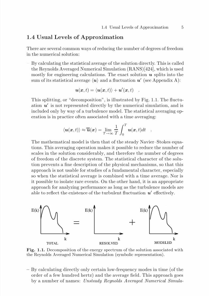
– By calculating the statistical average of the solution directly. This is calledthe Reynolds Averaged Numerical Simulation (RANS)[424], which is usedmostly for engineering calculations. The exact solution u splits into thesum of its statistical average u and a fluctuation u (see Appendix A):
u(x, t) = u(x, t) + u(x, t) .
This splitting, or “decomposition”, is illustrated by Fig. 1.1. The fluctu-
ation u is not represented directly by the numerical simulation, and isincluded only by way of a turbulence model. The statistical averaging op-eration is in practice often associated with a time averaging:
u(x, t) ≈ u(x) = limT →∞
1
T
T 0
u(x, t)dt .
The mathematical model is then that of the steady Navier–Stokes equa-tions. This averaging operation makes it possible to reduce the number of
scales in the solution considerably, and therefore the number of degreesof freedom of the discrete system. The statistical character of the solu-tion prevents a fine description of the physical mechanisms, so that thisapproach is not usable for studies of a fundamental character, especiallyso when the statistical average is combined with a time average. Nor isit possible to isolate rare events. On the other hand, it is an appropriateapproach for analyzing performance as long as the turbulence models areable to reflect the existence of the turbulent fluctuation u effectively.
Fig. 1.1. Decomposition of the energy spectrum of the solution associated withthe Reynolds Averaged Numerical Simulation (symbolic representation).
– By calculating directly only certain low-frequency modes in time (of theorder of a few hundred hertz) and the average field. This approach goesby a number of names: Unsteady Reynolds Averaged Numerical Simula-

7/21/2019 Large Eddy Simulation for Incompressible Flows
http://slidepdf.com/reader/full/large-eddy-simulation-for-incompressible-flows 31/573
6 1. Introduction
tion (URANS), Semi-Deterministic Simulation (SDS), Very Large-Eddy Simulation (VLES), and sometimes Coherent Structure Capturing (CSC)[726, 44]. The field u appears here as the sum of three contributing terms[456, 451, 240, 726]:
u(x, t) = u(x) + u(x, t)c + u(x, t) .
The first term is the time average of the exact solution, the second its con-ditional statistical average, and the third the turbulent fluctuation. Thisdecomposition is illustrated in Fig. 1.2. The conditional average is associ-ated with a predefined class of events. When these events occur at a settime period, this is a phase average. The u(x, t)c term is interpreted as
the contribution of the coherent modes to the flow dynamics, while theu term, on the other hand, is supposed to represent the random partof the turbulence. The variable described by the mathematical model isnow the sum u(x) + u(x, t)c, with the random part being representedby a turbulence model. It should be noted that, in the case where thereexists a deterministic low-frequency forcing of the solution, the conditionalaverage is conventionally interpreted as a phase average of the solution, fora frequency equal to that of the forcing term; but if this does not exist,the interpretation of the results is still open to debate. Since this is an un-
steady approach, it contains more information than the previous one; butit still precludes a deterministic description of a particular event. It is of use for analyzing the performance characteristics of systems in which theunsteady character is forced by some external action (such as periodicallypulsed flows).
Fig. 1.2. Decomposition of the energy spectrum of the solution associated with theUnsteady Reynolds Averaged Numerical Simulation approach, when a predominantfrequency exists (symbolic representation).
– By projecting the solution on the ad hoc function basis and retaining onlya minimum number of modes, to get a dynamical system with fewer degreesof freedom. The idea here is to find an optimum decomposition basis forrepresenting the phenomenon, in order to minimize the number of degreesof freedom in the discrete dynamical system. There is no averaging donehere, so the space-time and dynamics resolution of the numerical model is

7/21/2019 Large Eddy Simulation for Incompressible Flows
http://slidepdf.com/reader/full/large-eddy-simulation-for-incompressible-flows 32/573
1.4 Usual Levels of Approximation 7
still as fine as that of the continuum model, but is now optimized. Severalapproaches are encountered in practice.The first is to use standard basis function (Fourier modes in the spectralspace or polynomials in the physical space, for example) and distributethe degrees of freedom as best possible in space and time to minimize thenumber of them, i.e. adapt the space-time resolution of the simulation tothe nature of the solution. We thus adapt the topology of the discretedynamical system to that of the exact solution. This approach results inthe use of self-adapting grids and time steps in the physical space. It isnot associated with an operation to reduce the complexity by switching toa higher level of statistical description of the system. It leads to a much lessimportant reduction of the discrete system than those techniques based on
statistical averaging, and is limited by the complexity of the continuoussolution.Another approach is to use optimal basis functions, a small number of which will suffice for representing the flow dynamics. The problem is thento determine what these basis functions are. One example is the ProperOrthogonal Decomposition (POD) mode basis, which is optimum for rep-resenting kinetic energy (see [55] for a survey). This technique allows veryhigh data compression, and generates a dynamical system of very smalldimensions (a few dozen degrees of freedom at most, in practice). The ap-
proach is very seldom used because it requires very complete informationconcerning the solution in order to be able to determine the base functions.The various approaches above all return complete information concerningthe solutions of the exact problem, so they are perfectly suited to studiesof a fundamental nature. They may not, on the other hand, be optimal interms of reducing the complexity for certain engineering analyses that donot require such complete data.
– By calculating only the low-frequency modes in space directly. This is whatis done in Large-Eddy Simulation (LES). It is this approach that is dis-
cussed in the following. It is illustrated in Fig. 1.3.
Typical results obtained by these three approaches are illustrated inFig. 1.4.
Fig. 1.3. Decomposition of the energy spectrum in the solution associated withlarge-eddy simulation (symbolic representation).

7/21/2019 Large Eddy Simulation for Incompressible Flows
http://slidepdf.com/reader/full/large-eddy-simulation-for-incompressible-flows 33/573
8 1. Introduction
Fig. 1.4. Pressure spectrum inside a cavity. Top: experimental data (ideal direct-numerical simulation) (courtesy of L. Jacquin, ONERA); Middle : large-eddy simu-lation (Courtesy of L. Larcheveque, ONERA); Bottom : unsteady RANS simulation(Courtesy of V. Gleize, ONERA).

7/21/2019 Large Eddy Simulation for Incompressible Flows
http://slidepdf.com/reader/full/large-eddy-simulation-for-incompressible-flows 34/573
1.5 Large-Eddy Simulation: from Practice to Theory. Structure of the Book 9
1.5 Large-Eddy Simulation: from Practice to Theory.Structure of the Book
As mentioned above, the Large-Eddy Simulation approach relies on the def-inition of large and small scales. This fuzzy and empirical concept requiresfurther discussion to become a tractable tool from both the theoretical andpractical points of view. Bases for the theoretical understanding and modeling of this approach are now introduced. In practice, the Large-Eddy Simulationtechnique consists in solving the set of ad hoc governing equations on a com-putational grid which is too coarse to represent the smallest physical scales.Let ∆x and η be the computional mesh size (assumed to be uniform for thesake of simplicity) and the characteristic size of the smallest physical scales.Let u be the exact solution of the following continuous generic conservationlaw (the case of the Navier–Stokes equations will be extensively discussed inthe core of the book)
∂u
∂t + F (u, u) = 0 (1.2)
where F (·, ·) is a non-linear flux function. The Large-Eddy Simulation prob-
lem consists in finding the best approximation of u on the computational gridby solving the following discrete problem
δud
δt + F d(ud, ud) = 0 (1.3)
where ud, δ/δt and F d(·, ·) are the discrete approximations of u, ∂/∂t and
F (·, ·) on the computational grid, respectively. Thus, the question arise of defining what is the best possible approximation of u, uΠ , among all discretesolutions ud associated with ∆x.
Let e(u, ud) be a measure of the difference between u and ud, which doesnot need to be explicitely defined for the present purpose. It is just empha-sized here that since Large-Eddy Simulation is used to compute turbulentflows, u exhibits a chaotic behavior and therefore e(u, ud) should rely on sta-tistical moments of the solutions. A consistency constraint on the definitionof the error functional is that it must vanish in the limit case of the DirectNumerical Simulation
lim∆x−→η
e(u, ud) = 0 (1.4)
A careful look at the problem reveals that the error can be decomposedas
e(u, ud) = eΠ (u, ud) + ed(u, ud) + er(u, ud) (1.5)
where

7/21/2019 Large Eddy Simulation for Incompressible Flows
http://slidepdf.com/reader/full/large-eddy-simulation-for-incompressible-flows 35/573
10 1. Introduction
1. eΠ (u, ud) is the projection error which accounts for the fact that the exactsolution u is approximated using a finite number of degrees of freedom.The Nyquist theorem tells us that no scale smaller than 2∆x can becaptured in the simulation. As a consequence, ud can never be strictlyequal to u :
|u − ud| = 0 (1.6)
2. ed(u, ud) is the discretization error which accounts for the fact that par-tial derivatives which appear in the continuous problem are approximatedon the computational grid using Finite Diffrence, Finite Volume, FiniteElement (or other similar) schemes. Putting the emphasis on spatialderivatives, this is expressed as
F d(u, u) = F (u, u) (1.7)
3. er(u, ud) is the resolution error , which accounts for the fact that, somescales of the exact solution being missing, the evaluation of the non-linearflux function cannot be exact, even if the discretization error is driven tozero:
F (ud, ud) = F (u, u) (1.8)
This analysis shows that the Large-Eddy Simulation problem is very com-plex, since it depends explicitely on the exact solution, the computational gridand the numerical method, making each problem appearing as unique . There-fore, it is necessary to find some mathematical models for the Large-EddySimulation problem which will mimic its main features, the most importantone being the removal of the small scales of the exact solution. A simplifiedheuristic view of this problem is illustrated in Fig. 1.5, where the effect of theNyquist filter is represented.
Several mathematical models have been proposed to handle the true
Large-Eddy Simulation problem. The most popular one (see [216, 440, 495,619, 627]) relies on the representation of the removal of the small scales asthe result of the application of a low-pass convolution filter (in terms of wave number) to the exact solution. The definition and the properties of this filtering operator are presented in Chap. 2. The application of this filterto the Navier–Stokes equations, described in Chap. 3, yields the correspond-ing constitutive mathematical model for the large-eddy simulation. Alternatemathematical models are detailed in Chap. 4.
The second question raised by the Large-Eddy Simulation approach dealswith the search for the best approximate solution u
Π ∈ u
d that will mini-
mize the error e(u, ud). The short analysis given above shows that the projec-tion error, eΠ (u, ud) cannot be avoided. Therefore, the best, ideal Large-EddySolution is such that
e(u, ud) = e(u, uΠ ) = eΠ (u, uΠ ) (1.9)
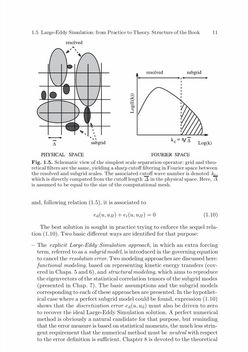
7/21/2019 Large Eddy Simulation for Incompressible Flows
http://slidepdf.com/reader/full/large-eddy-simulation-for-incompressible-flows 36/573
1.5 Large-Eddy Simulation: from Practice to Theory. Structure of the Book 11
Fig. 1.5. Schematic view of the simplest scale separation operator: grid and theo-retical filters are the same, yielding a sharp cutoff filtering in Fourier space betweenthe resolved and subgrid scales. The associated cutoff wave number is denoted kc,which is directly computed from the cutoff length ∆ in the physical space. Here, ∆
is assumed to be equal to the size of the computational mesh.
and, following relation (1.5), it is associated to
ed(u, uΠ ) + er(u, uΠ ) = 0 (1.10)
The best solution in sought in practice trying to enforce the sequel rela-tion (1.10). Two basic different ways are identified for that purpose:
– The explicit Large-Eddy Simulation approach , in which an extra forcingterm, referred to as a subgrid model , is introduced in the governing equationto cancel the resolution error . Two modeling approaches are discussed here:
functional modeling , based on representing kinetic energy transfers (cov-ered in Chaps. 5 and 6), and structural modeling , which aims to reproducethe eigenvectors of the statistical correlation tensors of the subgrid modes(presented in Chap. 7). The basic assumptions and the subgrid modelscorresponding to each of these approaches are presented. In the hypothet-ical case where a perfect subgrid model could be found, expression (1.10)shows that the discretization error e
d(u, u
d) must also be driven to zero
to recover the ideal Large-Eddy Simulation solution. A perfect numericalmethod is obviously a natural candidate for that purpose, but remindingthat the error measure is based on statistical moments, the much less strin-gent requirement that the numerical method must be neutral with respectto the error definition is sufficient. Chapter 8 is devoted to the theoretical
7/21/2019 Large Eddy Simulation for Incompressible Flows
http://slidepdf.com/reader/full/large-eddy-simulation-for-incompressible-flows 37/573
12 1. Introduction
problems related to the effects of the numerical method used in the simula-tion. The representation of the numerical error in the form of an additionalfilter is introduced, along with the problem of the relative weight of thevarious filters used in the numerical simulation.
– The implicit Large-Eddy Simulation approach , in which no extra term isintroduced in the governing equations, but the numerical method is chosensuch that the numerical error and the resolution error will cancel eachother, yielding a direct fulfilment of relation (1.10). This approach is brieflypresented in this book in Sect. 5.3.4. The interested reader can refer to [276]for an exhaustive description.
The fact that the ideal solution uΠ is associated to a non-vanishing pro-
jection error eΠ (u, uΠ ) raises the problem of the reliability of data obtainedvia Large-Eddy Simulation for practical purposes. Several theoretical andpractical problems are met when addressing the issue of validating and ex-ploiting Large-Eddy Simulation. The definition of the best solution beingintrinsically based on the definition of the error functional (which is arbi-trary), a universal answer seems to be meaningless. Questions concerning theanalysis and validation of the large-eddy simulation calculations are dealtwith in Chap. 9. The concept of statistically partially equivalent simulationsis introduced, which is of major importance to interpret the nature of the
data recovered from Large-Eddy Simulation. A short survey of available re-sults dealing with the properties of filtered Navier–Stokes solutions (ideallyuΠ ) and Large-Eddy Simulation solutions (true ud fields) is presented.
The discussions presented above deal with the definition of the Large-Eddy Simulation problem inside the computational domain. As all differentialproblems, it must be supplemented with ad hoc boundary conditions to yielda well-posed problem. Thus, the new question of defining discrete boundaryconditions in a consistent way appears. The problem is similar to the previousone: what boundary conditions should be used to reach the best solution uΠ ?
A weaker constraint is to find boundary conditions which do not deterioratethe accuracy that could potentially be reached with the selected numericalscheme and closure. The boundary conditions used for large-eddy simulationare discussed in Chap. 10, where the main cases treated are solid walls andturbulent inflow conditions. In the solid wall case, the emphasis is put on theproblem of defining wall stress models, which are subgrid models derived forthe specific purpose of taking into account the dynamics of the inner layerof turbulent boundary layers. The issue of defining efficient turbulent inflowcondtions raises from the need to truncate the computational domain, whichleads to the requirement of finding a way to take into account upstreamturbulent fluctuations in the boundary conditions.
Despite the fact that it yields very significant complexity reduction interms of degrees of freedom with respect to Direct Numerical Simulation,Large-Eddy Simulation still requires considerable computational efforts tohandle realistic applications. To obtain further complexity reduction, several

7/21/2019 Large Eddy Simulation for Incompressible Flows
http://slidepdf.com/reader/full/large-eddy-simulation-for-incompressible-flows 38/573
1.5 Large-Eddy Simulation: from Practice to Theory. Structure of the Book 13
hybridizations of the Large-Eddy Simulation technique have been proposed.Methods for reducing the cost of Large-Eddy Simulation by coupling it withmultiresolution and multidomain techniques are presented in Chap. 11. Hy-brid RANS/LES approaches are presented in Chap. 12. The definition of suchmultiresolution methods and/or hybrid RANS/LES techniques raises manypractical and theoretical issues. Among the most important ones, the empha-sis is put in the dedicated chapters on the coupling strategies and the factthat the instantaneous fields can be fully discontinuous (fully meaning herethat the velocity field is not a priori continuous at the interfaces betweendomains with different resolution, but also that even the number of spacedimension and the number of unknwons can be different).
Practical aspects concerning the implementation of subgrid models are de-
scribed in Chap. 13. Lastly, the discussion is illustrated by examples of large-eddy simulation applications for different categories of flows, in Chap. 14.
Chapter 15 is devoted the the extension of concepts, methods and modelspresented in previous chapters to the case of a more complex physical system,in which an additional equation for a scalar is added to the Navier–Stokesequations. Two cases are considered: the passive scalar case, in which thereis no feedback in the momentum equation and the new problem is restrictedto closing the filtered scalar equation, and the active scalar case, which corre-sponds to a two-way coupling between the scalar field and the velocity field.
In the latter, the definition of subgrid models for both the velocity and thescalar is a full problem. For the sake of clarity, the discussion is limited tostably stratified flows and buoyancy driven flows. Combustion and two-phaseflows are not treated.

7/21/2019 Large Eddy Simulation for Incompressible Flows
http://slidepdf.com/reader/full/large-eddy-simulation-for-incompressible-flows 39/573
2. Formal Introduction to Scale Separation:Band-Pass Filtering
The idea of scale separation introduced in the preceding chapter will now beformalized on the mathematical level, to show how to handle the equations
and derive the subgrid models.This chapter is devoted to the representation of the filtering as a con-
volution product, which is the most common way to model the removal of small scales in the Larg-Eddy Simulation approach. Other definitions, suchas partial statistical averaging or conditional averaging [251, 250, 465], willbe presented in Chap. 4. The filtering approach is first presented in the idealcase of a filter of uniform cutoff length over an infinite domain (Sect. 2.1).Fundamental properties of filters and their approximation via differential op-erators is presented. Extensions to the cases of a bounded domain and a filter
of variable cutoff length are then discussed (Sect. 2.2). The chapter is closedby discussing a few properties of the Eulerian time-domain filters (Sect. 2.3).
2.1 Definition and Properties of the Filterin the Homogeneous Case
The framework is restricted here to the case of homogeneous isotropic filters,for the sake of easier analysis, and to allow a better understanding of the
physics of the phenomena. The filter considered is isotropic . This means thatits properties are independent of the position and orientation of the frame of reference in space, which implies that it is applied to an unbounded domainand that the cutoff scale is constant and identical in all directions of space.This is the framework in which subgrid modeling developed historically. Theextension to anisotropic and inhomogeneous1 filters, which researchers haveonly more recently begun to look into, is described in Sect. 2.2.
2.1.1 Definition
Scales are separated by applying a scale high-pass filter, i.e. low-pass in fre-quency, to the exact solution. This filtering is represented mathematically in
1 That is, whose characteristics, such as the mathematical form or cutoff frequency,are not invariant by translation or rotation of the frame of reference in whichthey are defined.
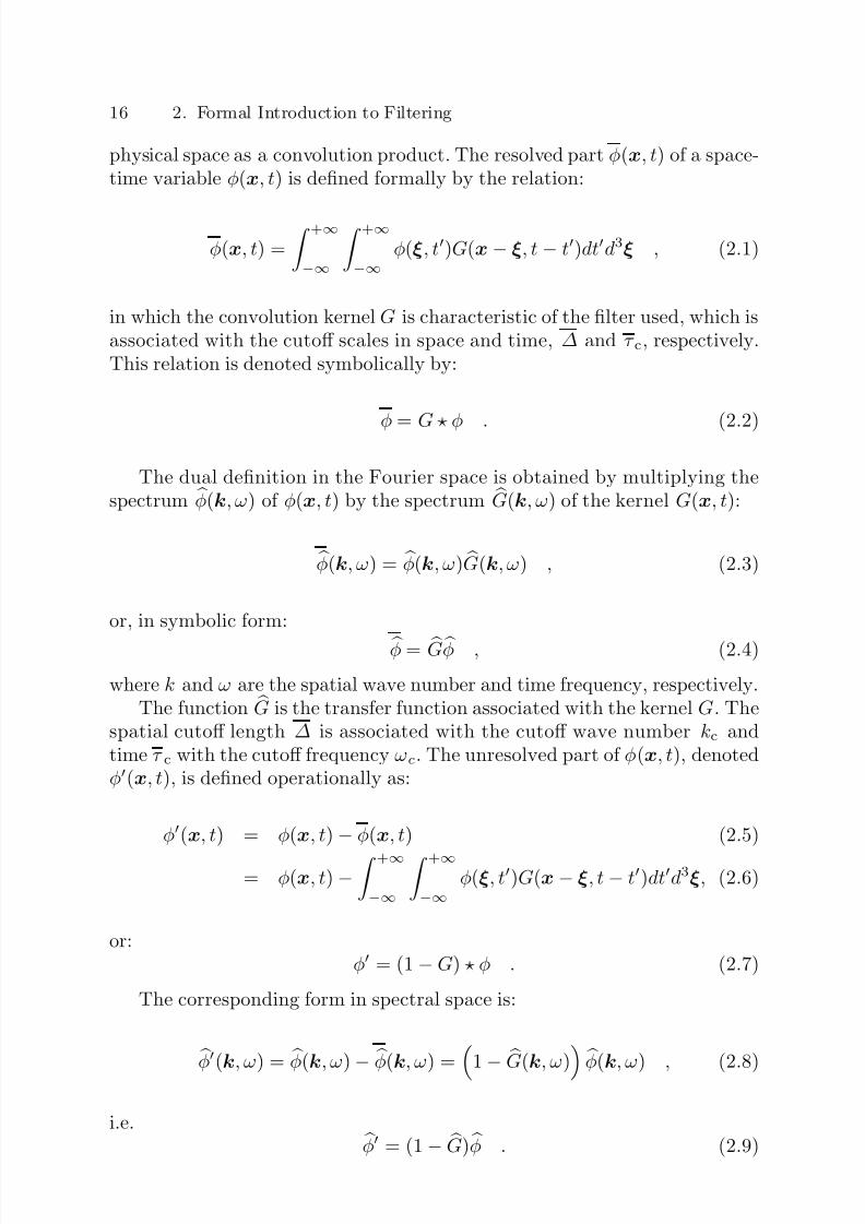
7/21/2019 Large Eddy Simulation for Incompressible Flows
http://slidepdf.com/reader/full/large-eddy-simulation-for-incompressible-flows 40/573
16 2. Formal Introduction to Filtering
physical space as a convolution product. The resolved part φ(x, t) of a space-time variable φ(x, t) is defined formally by the relation:
φ(x, t) =
+∞
−∞
+∞
−∞
φ(ξ, t)G(x − ξ, t − t)dtd3ξ , (2.1)
in which the convolution kernel G is characteristic of the filter used, which isassociated with the cutoff scales in space and time, ∆ and τ c, respectively.This relation is denoted symbolically by:
φ = G φ . (2.2)
The dual definition in the Fourier space is obtained by multiplying thespectrum φ(k, ω) of φ(x, t) by the spectrum G(k, ω) of the kernel G(x, t):
φ(k, ω) = φ(k, ω) G(k, ω) , (2.3)
or, in symbolic form: φ = G φ , (2.4)
where k and ω are the spatial wave number and time frequency, respectively.The function G is the transfer function associated with the kernel G. The
spatial cutoff length ∆ is associated with the cutoff wave number kc andtime τ c with the cutoff frequency ωc. The unresolved part of φ(x, t), denotedφ(x, t), is defined operationally as:
φ(x, t) = φ(x, t)
−φ(x, t) (2.5)
= φ(x, t) − +∞
−∞
+∞
−∞
φ(ξ, t)G(x − ξ, t − t)dtd3ξ, (2.6)
or:φ = (1 − G) φ . (2.7)
The corresponding form in spectral space is:
φ(k, ω) = φ(k, ω)− φ(k, ω) = 1
− G(k, ω) φ(k, ω) , (2.8)
i.e. φ = (1 − G) φ . (2.9)

7/21/2019 Large Eddy Simulation for Incompressible Flows
http://slidepdf.com/reader/full/large-eddy-simulation-for-incompressible-flows 41/573
2.1 Definition and Properties of the Filter in the Homogeneous Case 17
2.1.2 Fundamental Properties
In order to be able to manipulate the Navier–Stokes equations after applying
a filter, we require that the filter verify the three following properties:
1. Conservation of constants
a = a ⇐⇒ +∞
−∞
+∞
−∞
G(ξ, t)d3ξdt = 1 . (2.10)
2. Linearityφ + ψ = φ + ψ . (2.11)
This property is automatically satisfied, since the product of convolutionverifies it independently of the characteristics of the kernel G.
3. Commutation with derivation
∂φ
∂s =
∂φ
∂s, s = x, t . (2.12)
Introducing the commutator [f, g] of two operators f and g applied to thedummy variable φ
[f, g]φ ≡ f g(φ) − g f (φ) = f (g(φ)) − g(f (φ)) , (2.13)
the relation (2.12) can be re-written symbolicallyG,
∂
∂s
= 0 . (2.14)
The commutator defined by relation (2.13) has the followingproperties2:
[f, g] =
−[g, f ] Skew-symmetry , (2.15)
[f g, h] = [f, h] g + f [g, h] Leibniz identity , (2.16)
[f, [g, h]] + [g, [h, f ]] + [h, [f, g]] = 0 Jacobi’s identity . (2.17)
The filters that verify these three properties are not, in the general case,Reynolds operators (see Appendix A), i.e.
φ = G G φ = G2 φ = φ = G φ , (2.18)
φ = G (1 − G) φ = 0 , (2.19)
2 In the linear case, the commutator satisfies all the properties of the Poisson-bracket operator, as defined in classical mechanics.

7/21/2019 Large Eddy Simulation for Incompressible Flows
http://slidepdf.com/reader/full/large-eddy-simulation-for-incompressible-flows 42/573
18 2. Formal Introduction to Filtering
which is equivalent to saying that G is not a projector (excluding the trivialcase of the identity application). Let us recall that an application P is definedas being a projector if P
P = P . Such an application is idempotent because
it verifies the relation
P n ≡ P P ... P n times
= P, ∀n ∈ IN+ . (2.20)
When G is not a projector, the filtering can be interpreted as a change of variable, and can be inverted, so there is no loss of information3 [243]. Thekernel of the application is reduced to the null element, i.e. ker(G) = 0.
If the filter is a Reynolds operator, we get
G2 = 1 , (2.21)
or, remembering the property of conservation of constants:
G = 1 . (2.22)
In the spectral space, the idempotency property implies that the transferfunction takes the following form:
G(k, ω) = 0
1 ∀k,
∀ω . (2.23)
The convolution kernel G therefore takes the form of a sum of Dirac func-tions and Heaviside functions associated with non-intersecting domains. Theconservation of constants implies that G is 1 for the modes that are constantin space and time. The application can no longer be inverted because its ker-nel ker(G) = φ is no longer reduced to the zero element; and consequently,the filtering induces an irremediable loss of information.
A filter is said to be positive if:
G(x, t) > 0, ∀x and ∀t . (2.24)
2.1.3 Characterization of Different Approximations
The various methods mentioned in the previous section for reducing the num-ber of degrees of freedom will now be explained. We now assume that the
3 The reduction of the number of degrees of freedom comes from the fact that thenew variable, i.e. the filtered variable, is more regular than the original one inthe sense that it contains fewer high frequencies. Its characteristic scale in space
is therefore larger, which makes it possible to use a coarser solution to describeit, and therefore fewer degrees of freedom.The result is a direct numerical simulation of the smoothed variable. As in
all numerical simulations, a numerical cutoff is imposed by the use of a finitenumber of degrees of freedom. But in the case considered here the numericalcutoff is assumed to occur within the dissipative range of the spectrum, so thatno active scales are missing.

7/21/2019 Large Eddy Simulation for Incompressible Flows
http://slidepdf.com/reader/full/large-eddy-simulation-for-incompressible-flows 43/573
2.1 Definition and Properties of the Filter in the Homogeneous Case 19
space-time convolution kernel G(x−ξ, t−t) in IR4 is obtained by tensorizingmono-dimensional kernels:
G(x − ξ, t − t) = G(x − ξ)Gt(t − t) = Gt(t − t) i=1,3
Gi(xi − ξ i) . (2.25)
The Reynolds time average over a time interval T is found by taking:
Gt(t − t) = HT
T , Gi(xi − ξ i) = δ (xi − ξ i), i = 1, 2, 3 , (2.26)
in which δ is a Dirac function and HT the Heaviside function correspondingto the interval chosen. This average is extended to the ith direction of spaceby letting Gi(xi− ξ i) = HL/L, in which L is the desired integration interval.
The phase average corresponding to the frequency ωc is obtained by let-ting:
Gt(ω) = δ (ω − ωc), Gi(xi − ξ i) = δ (xi − ξ i), i = 1, 2, 3 . (2.27)
In all of the following, the emphasis will be put on the large-eddy simu-lation technique based on spatial filtering, because it is the most employedapproach, with very rare exceptions [160, 161, 603, 107]. This is expressed
by:Gt(t − t) = δ (t − t) . (2.28)
Different forms of the kernel Gi(xi − ξ i) in common use are describedin the following section. It should nonetheless be noted that, when a spatialfiltering is imposed, it automatically induces an implicit time filtering, sincethe dynamics of the Navier–Stokes equations makes it possible to associatea characteristic time with each characteristic length scale. This time scale isevaluated as follows. Let ∆ be the cutoff length associated with the filter, and
kc = π/∆ the associated wave number. Let E (k) be the energy spectrum of the exact solution (see Appendix A for a definition). The kinetic energy asso-ciated with the wave number kc is kcE (kc). The velocity scale vc associatedwith this same wave number is estimated as:
vc =
kcE (kc) . (2.29)
The characteristic time tc associated with the length ∆ is calculated bydimensional arguments as follows:
tc = ∆/vc . (2.30)
The corresponding frequency is ωc = 2π/tc. The physical analysis showsthat, for spectrum forms E (k) considered in the large-eddy simulation frame-work, vc is a monotonic decreasing function of kc (resp. monotonic increasing

7/21/2019 Large Eddy Simulation for Incompressible Flows
http://slidepdf.com/reader/full/large-eddy-simulation-for-incompressible-flows 44/573
20 2. Formal Introduction to Filtering
function of ∆), so that ωc is a monotonic increasing function of kc (resp.monotonic decreasing function of ∆). Suppressing the spatial scales corre-sponding to wave numbers higher than kc induces the disappearance of thetime frequencies higher than ωc. We nonetheless assume that the descriptionwith a spatial filtering alone is relevant.
Eulerian time-domain filtering for spatial large-eddy simulation is recov-ered taking
Gi(xi − ξ i) = δ (xi − ξ i) . (2.31)
A reasoning similar to the one given above shows that time filtering in-duces an implicit spatial filtering.
2.1.4 Differential Filters
A subset of the filters defined in the previous section is the set of differential filters [242, 243, 245, 248]. These filters are such that the kernel G is theGreen’s function associated to an inverse linear differential operator F :
φ = F (G φ) = F (φ)
= φ + θ∂φ
∂t + ∆l
∂φ
∂xl+ ∆lm
∂ 2φ
∂xl∂xm+ ... , (2.32)
where θ and ∆l are some time and space scales, respectively. Differential filterscan be grouped into several classes: elliptic, parabolic or hyperbolic filters. Inthe framework of a generalized space-time filtering, Germano [242, 243, 245]recommends using a parabolic or hyperbolic time filter and an elliptic spacefilter, for reasons of physical consistency with the nature of the Navier–Stokesequations. It is recalled that a filter is said to be elliptic (resp. parabolic orhyperbolic) if F is an elliptic (resp. parabolic, hyperbolic) operator. Examplesare given below [248].
Time Low-Pass Filter. A first example is the time low-pass filter. Theassociated inverse differential relation is:
φ = φ + θ∂φ
∂t . (2.33)
The corresponding convolution filter is:
φ = 1
θ t−∞ φ(x, t)exp−t−
t
θ dt . (2.34)
It is easily seen that this filter commutes with time and space deriva-tives. This filter is causal, because it incorporates no future information, andtherefore is applicable to real-time or post-processing of the data.
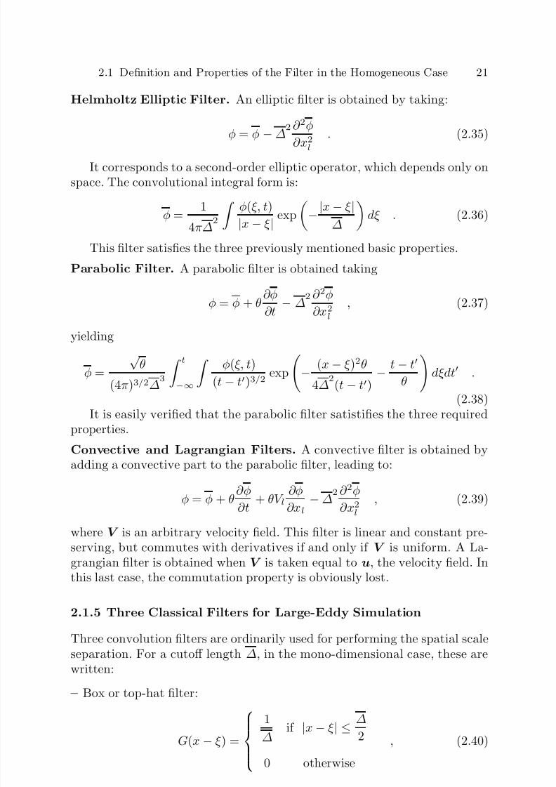
7/21/2019 Large Eddy Simulation for Incompressible Flows
http://slidepdf.com/reader/full/large-eddy-simulation-for-incompressible-flows 45/573
2.1 Definition and Properties of the Filter in the Homogeneous Case 21
Helmholtz Elliptic Filter. An elliptic filter is obtained by taking:
φ = φ − ∆
2 ∂ 2φ
∂x2l . (2.35)
It corresponds to a second-order elliptic operator, which depends only onspace. The convolutional integral form is:
φ = 1
4π∆2
φ(ξ, t)
|x − ξ | exp
−|x − ξ |
∆
dξ . (2.36)
This filter satisfies the three previously mentioned basic properties.
Parabolic Filter. A parabolic filter is obtained taking
φ = φ + θ∂φ
∂t − ∆
2 ∂ 2φ
∂x2l
, (2.37)
yielding
φ =
√ θ
(4π)3/2∆3
t−∞
φ(ξ, t)
(t − t)3/2 exp
− (x − ξ )2θ
4∆2
(t − t)− t − t
θ
dξdt .
(2.38)
It is easily verified that the parabolic filter satistifies the three requiredproperties.
Convective and Lagrangian Filters. A convective filter is obtained byadding a convective part to the parabolic filter, leading to:
φ = φ + θ∂φ
∂t + θV l
∂φ
∂xl− ∆
2 ∂ 2φ
∂x2l
, (2.39)
where V is an arbitrary velocity field. This filter is linear and constant pre-
serving, but commutes with derivatives if and only if V is uniform. A La-grangian filter is obtained when V is taken equal to u, the velocity field. Inthis last case, the commutation property is obviously lost.
2.1.5 Three Classical Filters for Large-Eddy Simulation
Three convolution filters are ordinarily used for performing the spatial scaleseparation. For a cutoff length ∆, in the mono-dimensional case, these arewritten:
– Box or top-hat filter:
G(x − ξ ) =
1
∆if |x − ξ | ≤ ∆
2
0 otherwise
, (2.40)

7/21/2019 Large Eddy Simulation for Incompressible Flows
http://slidepdf.com/reader/full/large-eddy-simulation-for-incompressible-flows 46/573
22 2. Formal Introduction to Filtering
G(k) =
sin(k∆/2)
k∆/2. (2.41)
The convolution kernel G and the transfer function G are represented inFigs. 2.1 and 2.2, respectively.
– Gaussian filter:
G(x − ξ ) =
γ
π∆2
1/2
exp
−γ |x − ξ |2
∆2
, (2.42)
G(k) = exp−∆
2k2
4γ , (2.43)
in which γ is a constant generally taken to be equal to 6. The convolutionkernel G and the transfer function G are represented in Figs. 2.3 and 2.4,respectively.
– Spectral or sharp cutoff filter:
G(x − ξ ) = sin(kc(x − ξ ))
kc(x−
ξ ) , with kc =
π
∆, (2.44)
G(k) =
1 if |k| ≤ kc
0 otherwise. (2.45)
The convolution kernel G and the transfer function G are represented inFigs. 2.5 and 2.6, respectively.
It is trivially verified that the first two filters are positive while the sharp
cutoff filter is not. The top-hat filter is local in the physical space (its supportis compact) and non-local in the Fourier space, inversely from the sharp cutoff filter, which is local in the spectral space and non-local in the physical space.As for the Gaussian filter, it is non-local both in the spectral and physicalspaces. Of all the filters presented, only the sharp cutoff has the property:
G · G... · G
n times
= Gn = G ,
and is therefore idempotent in the spectral space. Lastly, the top-hat andGaussian filters are said to be smooth because there is a frequency overlapbetween the quantities u and u.
Modification of the exact solution spectrum by the filtering operator isillustrated in figure 2.7.
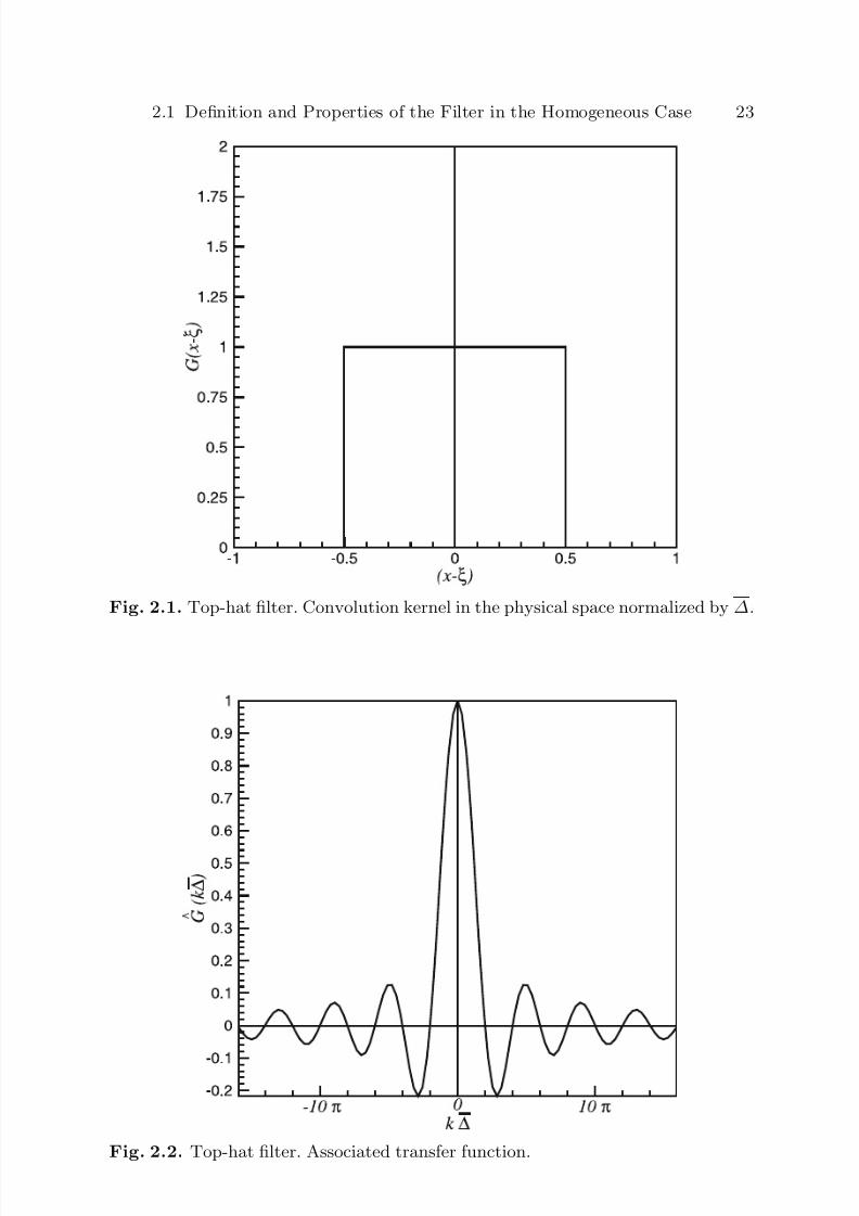
7/21/2019 Large Eddy Simulation for Incompressible Flows
http://slidepdf.com/reader/full/large-eddy-simulation-for-incompressible-flows 47/573
2.1 Definition and Properties of the Filter in the Homogeneous Case 23
Fig. 2.1. Top-hat filter. Convolution kernel in the physical space normalized by ∆.
Fig. 2.2. Top-hat filter. Associated transfer function.
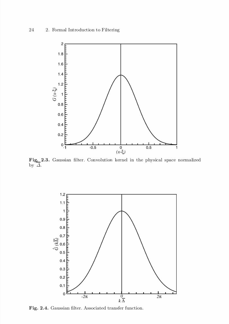
7/21/2019 Large Eddy Simulation for Incompressible Flows
http://slidepdf.com/reader/full/large-eddy-simulation-for-incompressible-flows 48/573
24 2. Formal Introduction to Filtering
Fig. 2.3. Gaussian filter. Convolution kernel in the physical space normalizedby ∆.
Fig. 2.4. Gaussian filter. Associated transfer function.

7/21/2019 Large Eddy Simulation for Incompressible Flows
http://slidepdf.com/reader/full/large-eddy-simulation-for-incompressible-flows 49/573
2.1 Definition and Properties of the Filter in the Homogeneous Case 25
Fig. 2.5. Sharp cutoff filter. Convolution kernel in the physical space.
Fig. 2.6. Sharp cutoff filter. Associated transfer function.

7/21/2019 Large Eddy Simulation for Incompressible Flows
http://slidepdf.com/reader/full/large-eddy-simulation-for-incompressible-flows 50/573
26 2. Formal Introduction to Filtering
Fig. 2.7. Energy spectrum of the unfiltered and filtered solutions. Filters consideredare a projective filter (sharp cutoff filter) and a smooth filter (Gaussian filter) withthe same cutoff wave number kc = 500.
2.1.6 Differential Interpretation of the Filters
General results. Convolution filters can be approximated as simple differ-ential operators via a Taylor series expansion, if some additional constraintsare fulfilled by the convolution kernel, thus yielding simplified and local fil-tering operators. Validation of the use of Taylor series expansions in the
representation of the filtering operator and conditions for convergence willbe discussed in the next section.
We first consider space filtering and recall its definition using a convolutionproduct:
φ(x, t) =
+∞
−∞
φ(ξ, t)G(x − ξ )dξ . (2.46)
To obtain a differential interpretation of the filter, we perform a Taylorseries expansion of the φ(ξ, t) term at (x, t):
φ(ξ, t) = φ(x, t) + (ξ − x) ∂φ(x, t)∂x
+ 12
(ξ − x)2 ∂ 2φ(x, t)∂x2
+ ... (2.47)
Introducing this expansion into (2.46), and considering the symmetry andconservation properties of the constants of the kernel G, we get:

7/21/2019 Large Eddy Simulation for Incompressible Flows
http://slidepdf.com/reader/full/large-eddy-simulation-for-incompressible-flows 51/573
2.1 Definition and Properties of the Filter in the Homogeneous Case 27
φ(x, t) = φ(x, t)1
2
∂ 2φ(x, t)
∂x2
+∞
−∞
z2G(z)dz + ...
+ 1n!
∂ n
φ(x, t)∂xn
znG(z)dz + ...
= φ(x, t) +l=1,∞
α(l)
l!
∂ lφ(x, t)
∂xl , (2.48)
where α(l) designates the lth-order moment of the convolution kernel:
α(l) = (−1)l +∞
−∞
zlG(z)dz . (2.49)
Assuming that the solution is 2π-periodic, the moments of the convolutionkernel can be rewritten as follows [728, 607]:
α(l) = ∆lM l, M l =
(−π−x)/∆
(π−x)/∆
ξ lG(ξ )dξ , (2.50)
leading to the following expression for the filtered variable φ:
φ(x) =
∞
k=0
(
−1)k
k! ∆
k
M k(x)
∂ kφ
∂xk (x) . (2.51)
With this relation, we can interpret the filtering as the application of a differential operator to the primitive variable φ. The subgrid part can alsobe rewritten using the following relation
φ(x) = φ(x) − φ(x)
= −
l=1,∞
α(l)
l!
∂ lφ(x)
∂xl
=∞k=1
(−1)k+1
k! ∆
kM k(x)
∂ kφ
∂xk (x) . (2.52)
The filtered variable φ can also be expanded using derivatives of the trans-fer function G of the filter [607]. Assuming periodicity and differentiabilityof φ, we can write
φ(x) =+∞
k=−∞
φkeıkx , ı2 =
−1 , (2.53)
and∂ lφ
∂xl(x) =
+∞k=−∞
(ık)lφkeıkx . (2.54)

7/21/2019 Large Eddy Simulation for Incompressible Flows
http://slidepdf.com/reader/full/large-eddy-simulation-for-incompressible-flows 52/573
28 2. Formal Introduction to Filtering
The filtered field is expanded as follows:
φ(x) =
+∞k=−∞
G(k)φkeıkx . (2.55)
The filtered field can be expressed as a Taylor series expansion in the filterwidth ∆:
φ(x, ∆) = φ(x, 0) + ∆ ∂φ
∂∆(x, 0) +
∆2
2
∂ 2φ
∂∆2 (x, 0) + ... . (2.56)
By differentiating (2.55) with respect to ∆, we obtain
∂ lφ
∂∆l
(x, 0) = l!al∂ lφ
∂xl(x) , (2.57)
with
al = 1
ıll!
∂ l G
∂kl (0) . (2.58)
The resulting final expression of the filtered field is
φ(x) =∞l=0
+∞k=−∞
(k∆)ll!
∂ l G∂kl
(0)φkeıkx . (2.59)
Time-domain filters defined as a convolution product can be expanded inan exactly similar way, yielding
φ(x, t) =
+∞
−∞
φ(x, t)G(t − t)dt
= φ(x, t) + l=1,∞
α(l)
l!
∂ lφ(x, t)
∂tl , (2.60)
The values of the first moments of the box and Gaussian filters are givenin Table 2.1. It can be checked that the sharp cutoff filter leads to a divergentseries, because of its non-localness.
For these two filters, we have the estimate
α(n) = O(∆n
) (2.61)
for space-domain filtering, and
α(n) = O(τ cn) (2.62)
for time-domain filtering.
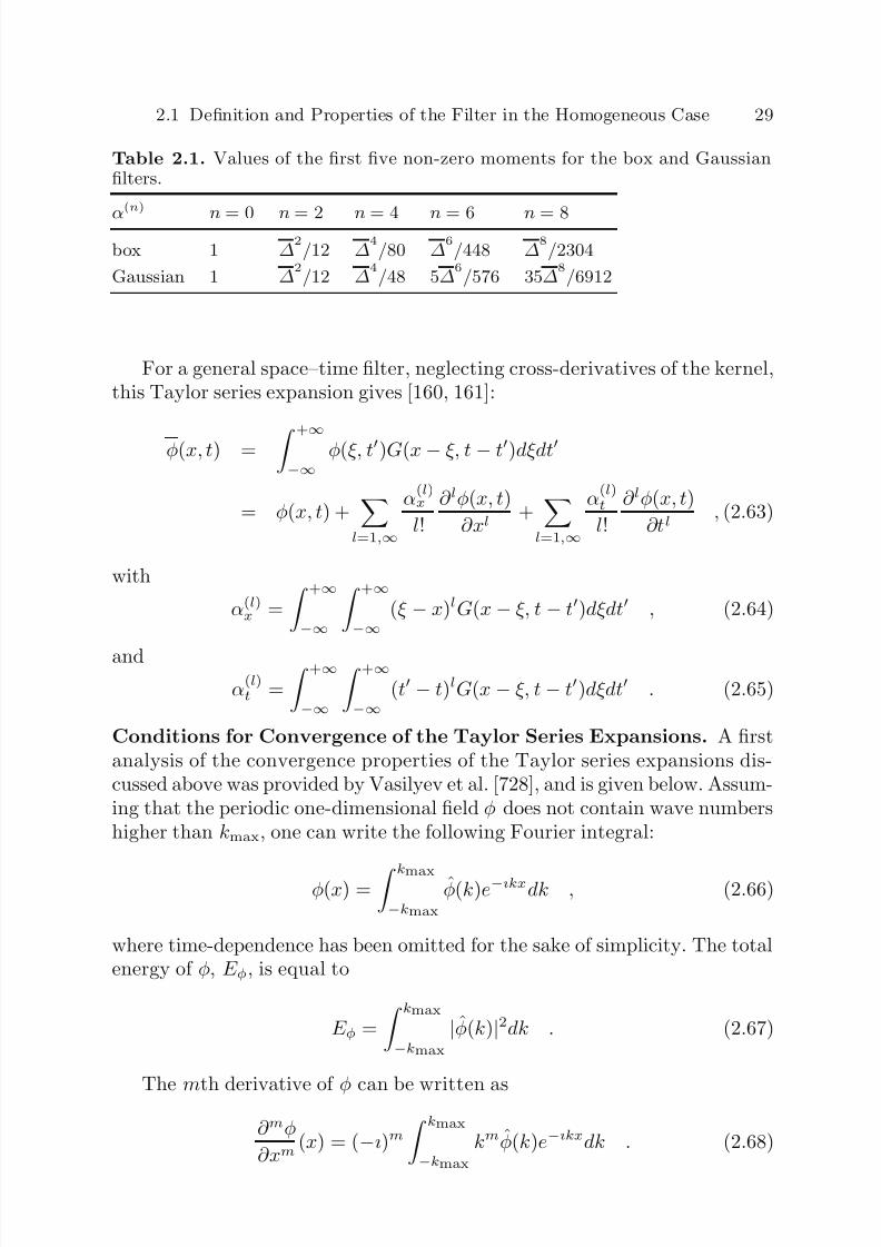
7/21/2019 Large Eddy Simulation for Incompressible Flows
http://slidepdf.com/reader/full/large-eddy-simulation-for-incompressible-flows 53/573
2.1 Definition and Properties of the Filter in the Homogeneous Case 29
Table 2.1. Values of the first five non-zero moments for the box and Gaussianfilters.
α(n)
n = 0 n = 2 n = 4 n = 6 n = 8
box 1 ∆2
/12 ∆4
/80 ∆6
/448 ∆8
/2304
Gaussian 1 ∆2
/12 ∆4
/48 5∆6
/576 35∆8
/6912
For a general space–time filter, neglecting cross-derivatives of the kernel,this Taylor series expansion gives [160, 161]:
φ(x, t) = +∞
−∞
φ(ξ, t)G(x − ξ, t − t)dξdt
= φ(x, t) +l=1,∞
α(l)x
l!
∂ lφ(x, t)
∂xl +
l=1,∞
α(l)t
l!
∂ lφ(x, t)
∂tl , (2.63)
with
α(l)x =
+∞
−∞
+∞
−∞
(ξ − x)lG(x − ξ, t − t)dξdt , (2.64)
andα
(l)t =
+∞
−∞
+∞
−∞
(t − t)lG(x − ξ, t − t)dξdt . (2.65)
Conditions for Convergence of the Taylor Series Expansions. A firstanalysis of the convergence properties of the Taylor series expansions dis-cussed above was provided by Vasilyev et al. [728], and is given below. Assum-ing that the periodic one-dimensional field φ does not contain wave numbershigher than kmax, one can write the following Fourier integral:
φ(x) = kmax
−kmax
φ(k)e−ıkxdk , (2.66)
where time-dependence has been omitted for the sake of simplicity. The totalenergy of φ, E φ, is equal to
E φ =
kmax
−kmax
|φ(k)|2dk . (2.67)
The mth derivative of φ can be written as
∂ mφ
∂xm(x) = (−ı)m
kmax
−kmax
kmφ(k)e−ıkxdk . (2.68)

7/21/2019 Large Eddy Simulation for Incompressible Flows
http://slidepdf.com/reader/full/large-eddy-simulation-for-incompressible-flows 54/573
30 2. Formal Introduction to Filtering
From this expression, we get the following bounds for the derivative:
∂ mφ
∂xm ≤ kmax
−kmax |k|2m
|φ(k)|2
dk
≤ kmax
−kmax
|k|mdk
1/2 kmax
−kmax
|φ(k)|dk
1/2
≤
2E φkmax
2m + 1 kmmax . (2.69)
From relations (2.69) and (2.51) we obtain the following inequalities:
∞l=0
(−1)l
l! ∆
lM l(x)
∂ lφ
∂xl (x)
≤ ∞l=0
1
l!∆l|M l(x)| ∂ lφ
∂xl(x)
≤ 2E φkmax
∞l=0
kmax∆
l |M l(x)|l!√
2l + 1.(2.70)
From this last inequality, it can easily be seen that the series (2.51) con-verges for any value of ∆ if the following constraint is satisfied:
liml−→∞
|M l+1(x)||M l(x)|(l + 1) = 0 . (2.71)
For filters with compact support, the following criterion holds:
liml−→∞
(kmax∆)|M l+1(x)||M l(x)|(l + 1)
< 1 . (2.72)
For symmetric filters, the analogous criterion is
liml−→∞
(kmax∆)2
|M 2l+2(x)||M 2l(x)|(2l + 2)(2l + 1) < 1 . (2.73)
Pruett et al. [607] proved that all symmetric, non-negative4 filters satisfyrelation (2.73). This proof is now presented. If the filter is non-negative,following an integral mean value theorem, there exists a value c, −2π ≤−π − x ≤ c ≤ π − x ≤ 2π, such that
|M 2l+2| = |c|∆
2
(−π−x)/∆
(π−x)/∆
ξ 2lG(ξ )dξ =
|c|∆
2
|M 2l| , (2.74)
4 It is recalled that the filter is said to be non-negative if G(x) ≥ 0, ∀x.
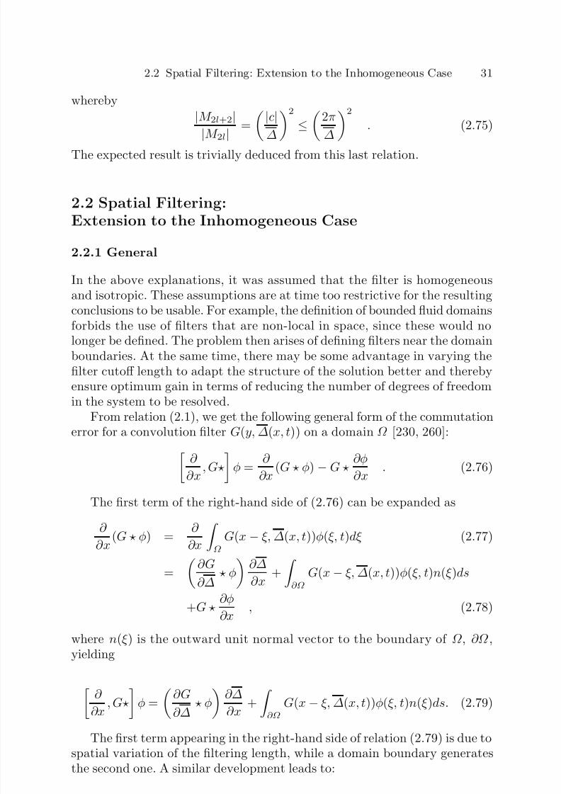
7/21/2019 Large Eddy Simulation for Incompressible Flows
http://slidepdf.com/reader/full/large-eddy-simulation-for-incompressible-flows 55/573
2.2 Spatial Filtering: Extension to the Inhomogeneous Case 31
whereby
|M 2l+2|
|M 2l| =
|c|
∆2
≤ 2π
∆ 2
. (2.75)
The expected result is trivially deduced from this last relation.
2.2 Spatial Filtering:Extension to the Inhomogeneous Case
2.2.1 General
In the above explanations, it was assumed that the filter is homogeneousand isotropic. These assumptions are at time too restrictive for the resultingconclusions to be usable. For example, the definition of bounded fluid domainsforbids the use of filters that are non-local in space, since these would nolonger be defined. The problem then arises of defining filters near the domainboundaries. At the same time, there may be some advantage in varying thefilter cutoff length to adapt the structure of the solution better and therebyensure optimum gain in terms of reducing the number of degrees of freedomin the system to be resolved.
From relation (2.1), we get the following general form of the commutationerror for a convolution filter G(y, ∆(x, t)) on a domain Ω [230, 260]:
∂
∂x, G
φ =
∂
∂x(G φ) − G
∂φ
∂x . (2.76)
The first term of the right-hand side of (2.76) can be expanded as
∂
∂x(G φ) =
∂
∂x ΩG(x − ξ, ∆(x, t))φ(ξ, t)dξ (2.77)
=∂G
∂∆ φ ∂∆
∂x + ∂Ω
G(x − ξ, ∆(x, t))φ(ξ, t)n(ξ )ds
+G ∂φ
∂x , (2.78)
where n(ξ ) is the outward unit normal vector to the boundary of Ω , ∂Ω ,yielding
∂ ∂x
, Gφ = ∂G∂∆
φ ∂∆∂x
+ ∂Ω
G(x − ξ, ∆(x, t))φ(ξ, t)n(ξ )ds. (2.79)
The first term appearing in the right-hand side of relation (2.79) is due tospatial variation of the filtering length, while a domain boundary generatesthe second one. A similar development leads to:
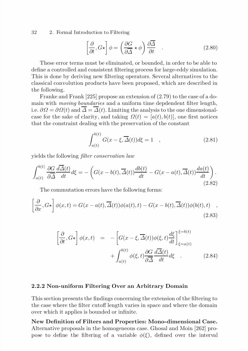
7/21/2019 Large Eddy Simulation for Incompressible Flows
http://slidepdf.com/reader/full/large-eddy-simulation-for-incompressible-flows 56/573
32 2. Formal Introduction to Filtering∂
∂t, G
φ =
∂G
∂∆ φ
∂∆
∂t . (2.80)
These error terms must be eliminated, or bounded, in order to be able todefine a controlled and consistent filtering process for large-eddy simulation.This is done by deriving new filtering operators. Several alternatives to theclassical convolution products have been proposed, which are described inthe following.
Franke and Frank [225] propose an extension of (2.79) to the case of a do-main with moving boundaries and a uniform time depdendent filter length,i.e. ∂Ω = ∂Ω (t) and ∆ = ∆(t). Limiting the analysis to the one dimensional-case for the sake of clarity, and taking Ω (t) = [a(t), b(t)], one first notices
that the constraint dealing with the preservation of the constant b(t)
a(t)
G(x − ξ, ∆(t))dξ = 1 , (2.81)
yields the following filter conservation law b(t)
a(t)
∂G
∂∆
d∆(t)
dt dξ = −
G(x − b(t), ∆(t))
db(t)
dt − G(x − a(t), ∆(t))
da(t)
dt
.
(2.82)The commutation errors have the following forms: ∂
∂x, G
φ(x, t) = G(x − a(t), ∆(t))φ(a(t), t) − G(x − b(t), ∆(t))φ(b(t), t) ,
(2.83)
∂
∂t, G
φ(x, t) = −
G(x − ξ, ∆(t))φ(ξ, t)
dξ
dt ξ=b(t)
ξ=a(t)
+ b(t)
a(t)
φ(ξ, t)∂G
∂∆
d∆(t)
dt dξ . (2.84)
2.2.2 Non-uniform Filtering Over an Arbitrary Domain
This section presents the findings concerning the extension of the filtering to
the case where the filter cutoff length varies in space and where the domainover which it applies is bounded or infinite.
New Definition of Filters and Properties: Mono-dimensional Case.Alternative proposals in the homogeneous case. Ghosal and Moin [262] pro-pose to define the filtering of a variable φ(ξ ), defined over the interval

7/21/2019 Large Eddy Simulation for Incompressible Flows
http://slidepdf.com/reader/full/large-eddy-simulation-for-incompressible-flows 57/573
2.2 Spatial Filtering: Extension to the Inhomogeneous Case 33
] − ∞, +∞[, as
φ(ξ ) = G φ =
1
∆ +∞
−∞ Gξ
−η
∆ φ(η)dη , (2.85)
in which the cutoff length ∆ is constant. The convolution kernel G is madeto verify the following four properties:
1. SymmetryG(−ξ ) = G(ξ ) . (2.86)
We note that this property was not explicitly required before, but thatit is verified by the three filters described in Sect. 2.1.5.
2. Conservation of constants +∞
−∞
a G(ξ )dξ, a = const. (2.87)
3. Fast decay. G(ξ ) → 0 as |ξ | → ∞ fast enough for all of its moments tobe finite, i.e. +∞
−∞
G(ξ )ξ ndξ < ∞, ∀n ≥ 0 . (2.88)
4. Quasi-local in physical space. G(ξ ) is localized (in a sense to be specified)in the interval [−1/2, 1/2].
Extension of the Top-Hat Filter to the Inhomogeneous Case: Prop-erties. Considering definition (2.85), the top-hat filter (2.40) is expressed:
G(ξ ) =
1 if |ξ | ≤ 1
20 otherwise
. (2.89)
There are a number of ways of extending this filter to the inhomogeneouscase. The problem posed is strictly analogous to that of extending finite vol-ume type schemes to the case of inhomogeneous structured grids: the controlvolumes can be defined directly on the computational grid or in a referencespace carrying a uniform grid, after a change of variable. Two extensionsof the box filter are discussed in the following, each based on a differentapproach.
Direct extension. If the cutoff length varies in space, one solution is to say:
φ(ξ ) = 1∆+(ξ ) + ∆−(ξ ) ξ+∆+(ξ)
ξ−∆−(ξ)φ(η)dη , (2.90)
in which ∆+(ξ ) and ∆−(ξ ) are positive functions and (∆+(ξ ) + ∆−(ξ )) is thecutoff length at point ξ . These different quantities are represented in Fig. 2.8.

7/21/2019 Large Eddy Simulation for Incompressible Flows
http://slidepdf.com/reader/full/large-eddy-simulation-for-incompressible-flows 58/573
34 2. Formal Introduction to Filtering
Fig. 2.8. Direct extension of the top-hat filter. Representation of the integrationcell at point ξ.
If the domain is finite or semi- infinite, the functions ∆+(ξ ) and ∆−(ξ ) mustdecrease fast enough near the domain boundaries for the integration interval[ξ −∆−(ξ ), ξ +∆+(ξ )] to remain defined. The box filter is extended intuitivelyhere, as an average over the control cell [ξ −∆−(ξ ), ξ +∆+(ξ )]. This approach
is similar to the finite volume techniques based on control volumes defineddirectly on the computational grid.
It is shown that this expression does not ensure the commutation propertywith derivation in space. Relation (2.12) becomes (the dependency of thefunctions ∆+ and ∆− as a function of ξ is not explicitly state, to streamlinethe notation):
G, d
dξ
φ =
(d/dξ ) (∆− + ∆+)
∆− + ∆+
φ
− 1∆+ + ∆−
φ(ξ + ∆+) d∆+
dξ + φ(ξ −∆−) d∆−
dξ .
(2.91)
The amplitude of the error committed cannot be evaluated a priori, andthus cannot be neglected. Also, when (2.90) is applied to the Navier–Stokesequations, all the terms, including the linear ones, will introduce unknownterms that will require a closure.
Extension by Variable Change. SOCF. To remedy this problem, a moregeneral alternative description than relation (2.90) is proposed by Ghosal andMoin [262]. This new definition consists of defining filters that commute atthe second order with the derivation in space (Second Order CommutingFilter, or SOCF). This is based on a change of variable that allows the use of a homogeneous filter. The function φ is assumed to be defined over a finiteor infinite interval [a, b]. Any regular monotonic function defined over thisinterval can be related to a definite function over the interval [−∞, +∞] byperforming the variable change:
ξ = f (x) , (2.92)
in which f is a strictly monotonic differentiable function such that:
f (a) = −∞, f (b) = +∞ . (2.93)

7/21/2019 Large Eddy Simulation for Incompressible Flows
http://slidepdf.com/reader/full/large-eddy-simulation-for-incompressible-flows 59/573
2.2 Spatial Filtering: Extension to the Inhomogeneous Case 35
The constant cutoff length ∆ defined over the reference space [−∞, +∞]is associated with the variable cutoff length δ (x) over the starting interval bythe relation:
δ (x) = ∆f (x)
. (2.94)
In the case of a finite or semi-infinite domain, the function f takes infinitevalues at the bounds and the convolution kernel becomes a Dirac function.The filtering of a function ψ(x) is defined in the inhomogeneous case in threesteps:
1. We perform the variable change x = f −1(ξ ), which leads to the definitionof the function φ(ξ ) = ψ(f −1(ξ )).
2. The function φ(ξ ) is then filtered by the usual homogeneous filter (2.85):
ψ(x) ≡ φ(ξ ) = 1
∆
+∞
−∞
G
f (x) − η
∆
φ(η)dη . (2.95)
3. The filtered quantity is then re-expressed in the original space:
ψ(x) = 1
∆
ba
G
f (x) − f (y)
∆
ψ(y)f (y)dy . (2.96)
This new expression of the filter modifies the commutation error with thespatial derivation. Using (2.95) and integrating by parts, we get:
dψ
dx = −f (x)
∆
G
f (x) − f (y)
∆
ψ(y)
y=b
y=a
+ 1
∆
ba
G
f (x) − f (y)
∆
f (x)ψ(y)dy . (2.97)
The fast decay property of the kernel G makes it possible to cancel thefirst term of the rigth-hand side. The commutation error is:
G, d
dξ
φ =
1
∆
ba
G
f (x) − f (y)
∆
f (y)ψ(y)
×
1 − f (x)
f (y)
dy . (2.98)
In order to simplify this expression, we introduce a new variable ζ such
that: f (y) = f (x) + ∆ζ . (2.99)
The variable y is then re-expressed as a series as a function of ∆:
y = y0(ζ ) + ∆y1(ζ ) + ∆2
y2(ζ ) + ... (2.100)

7/21/2019 Large Eddy Simulation for Incompressible Flows
http://slidepdf.com/reader/full/large-eddy-simulation-for-incompressible-flows 60/573
36 2. Formal Introduction to Filtering
Then, combining relations (2.99) and (2.100), we get (the dependence of the functions according to the variable x is not explicitly shown, to streamlinethe notation):
y = x + ∆ζ
f − ∆
2f ζ
2f 3 + ... , (2.101)
which allows us to re-write relation (2.98) as:
G,
d
dξ
φ =
+∞
−∞
G(ζ )ψ(y(ζ ))
1 − f (x)
f (y(ζ ))
dζ (2.102)
= C 1∆ + C 2∆2
+ ... , (2.103)
in which the coefficients C 1 and C 2 are expressed as:
C 1 = f ψ
f 2
+∞
−∞
ζG(ζ )dζ , (2.104)
C 2 = 2f f ψ + f f ψ − 3f 2ψ
2f 4
+∞
−∞
ζ 2G(ζ )dζ . (2.105)
The symmetry property of the kernel G implies C 1 = 0, which ensuresthat the filter commutation error with the spatial derivation is of the secondorder as a function of the cutoff length ∆. The authors call this Second-OrderCommuting Filter (SOCF).
A study of the spectral distribution of the commutation error is availablein reference [262]. Rather than detailing this analysis here, only the majorresults will be explained. Considering a function of the form:
ψ(x) = ψkeıkx, ı2 = −1 , (2.106)
the two derivation operations are written:
dψ
dx = ıkψ,
dψ
dx = ıkψ . (2.107)
The commutation error can be measured by comparing the two wavenumbers k and k, the latter being such that ıkψ = ık ψ. The commutationerror is zero if k = k. Algebraic manipulations lead to the relation:
k
k = 1 − ı∆
f
f 2
+∞
−∞
ζG(ζ )sin(k∆ζ/f )dζ +∞
−∞
G(ζ )cos(k∆ζ/f )dζ
. (2.108)

7/21/2019 Large Eddy Simulation for Incompressible Flows
http://slidepdf.com/reader/full/large-eddy-simulation-for-incompressible-flows 61/573
2.2 Spatial Filtering: Extension to the Inhomogeneous Case 37
Using the modal decomposition (2.106), the commutation error can beexpressed in differential form. The calculations lead to:
G,
d
dx
ψ = α(2) f
f 3∆
2 d2ψ
dx2 + O(k∆)4 (2.109)
= −α(2)δ 2
δ
δ
d2ψ
dx2 + O(kδ )4 , (2.110)
in which δ (x) is the local cutoff length and α(2) the second-order moment of G, i.e.
α(2) = +∞
−∞
ζ 2G(ζ )dζ . (2.111)
Van der Ven’s Filters. Commuting filters can be defined with the spatialderivation at an order higher than 2, at least in the case of an infinite domain.To obtain such filters, Van der Ven [725] proposes defining the filtering forthe case of a variable cutoff length δ (x) by direct extension of the form (2.85):
φ(x) = 1
δ (x)
+∞
−∞
G
x − y
δ (x)
φ(y)dy . (2.112)
The function G is assumed here to be class C 1, symmetrical, and mustconserve the constants. Also, the function δ (x) is also assumed to be class C 1.This definition is achieved by linearizing the general formula (2.96) around x,that is by letting φ(y) = φ(x) and φ(x) − φ(y) = φ(x)(x − y) and includingrelation (2.94). This linearization operation is equivalent to considering thatthe function φ is linear in a neighbourhood of x containing the support of the convolution kernel. By introducing the variable change y = x −ζδ (x), thecorresponding commutation error is expressed:
G, ddxφ = δ
δ (G(ζ ) + ζG(ζ )) φ(x − ζδ (x))dζ . (2.113)
To increase the order of the commutation error, we look for functions Gthat are solutions to the equation
G + ζG = a G(n), n > 1 , (2.114)
in which a is a real and G(n) designates the nth derivative of the kernel G.For such functions, the commutation error becomes:
G, d
dx
φ = a
δ
δ (−1)n
G(ζ )
∂
∂ζ
nφ(x − ζδ (x))dζ (2.115)
= aδ (x)δ (x)n−1φ(n)(x) , (2.116)

7/21/2019 Large Eddy Simulation for Incompressible Flows
http://slidepdf.com/reader/full/large-eddy-simulation-for-incompressible-flows 62/573
38 2. Formal Introduction to Filtering
Fig. 2.9. High-order commuting filter. Graph of the associated transfer functionfor different values of the parameter m.
and is thus formally of order n − 1. Simple analysis shows that the Fouriertransform G of the solution to problem (2.114) verifying the constant con-servation property is of the form:
G(k) = exp
−aın
n kn
. (2.117)
The symmetry property of G implies that n = 2m is even, and therefore:
G(k) = exp
−a(−1)m
2m k2m
. (2.118)
The fast decay property is recovered for a = b(−1)m, b > 0. It can be seenthat the Gaussian filter then occurs again by letting m = 1. It is importantto note that this analysis is valid only for infinite domains, because when thebounds of the fluid domain are included they bring out additional error termswith which it is no longer possible to be sure of the order of the commutationerror. The transfer function obtained for various values of the parameter mis represented in Fig. 2.9.
High-Order Commuting Filters. Van der Ven’s analysis has been gen-
eralized by Vasilyev et al. [728] so as to contain previous works (SOCF andVan der Ven’s filters) as special cases. As for SOCF, the filtering process isdefined thanks to the use of a reference space. We now consider that thephysical domain [a, b] is mapped into the domain [α, β ]. Ghosal and Moinused α = −∞ and β = +∞. The correspondances between the two domainsare summarized in Table 2.2.
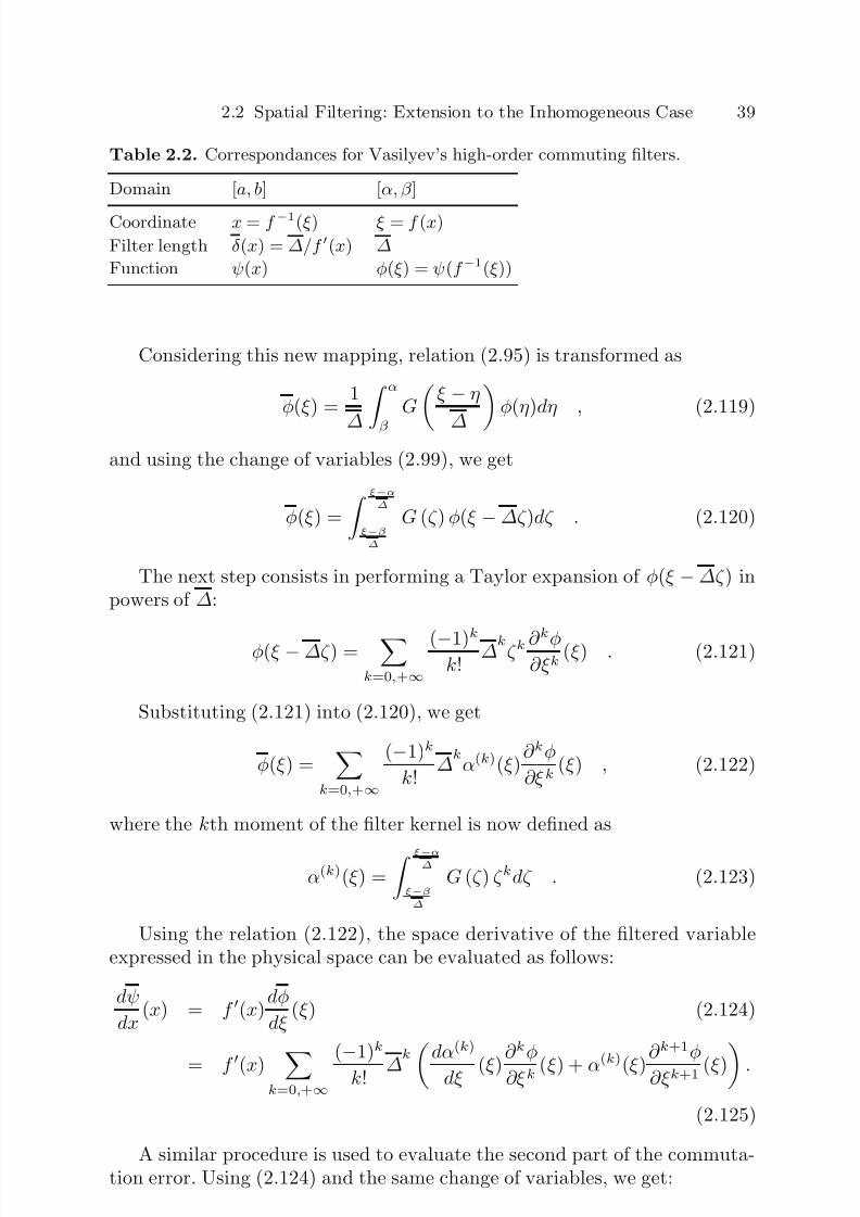
7/21/2019 Large Eddy Simulation for Incompressible Flows
http://slidepdf.com/reader/full/large-eddy-simulation-for-incompressible-flows 63/573
2.2 Spatial Filtering: Extension to the Inhomogeneous Case 39
Table 2.2. Correspondances for Vasilyev’s high-order commuting filters.
Domain [a, b] [α, β ]
Coordinate x = f −1(ξ) ξ = f (x)
Filter length δ (x) = ∆/f (x) ∆
Function ψ(x) φ(ξ) = ψ(f −1(ξ))
Considering this new mapping, relation (2.95) is transformed as
φ(ξ ) = 1
∆ α
β
Gξ − η
∆ φ(η)dη , (2.119)
and using the change of variables (2.99), we get
φ(ξ ) =
ξ−α∆
ξ−β
∆
G (ζ ) φ(ξ − ∆ζ )dζ . (2.120)
The next step consists in performing a Taylor expansion of φ(ξ − ∆ζ ) inpowers of ∆:
φ(ξ − ∆ζ ) = k=0,+∞
(−1)kk!
∆kζ k ∂ kφ∂ξ k
(ξ ) . (2.121)
Substituting (2.121) into (2.120), we get
φ(ξ ) =
k=0,+∞
(−1)k
k! ∆
kα(k)(ξ )
∂ kφ
∂ξ k (ξ ) , (2.122)
where the kth moment of the filter kernel is now defined as
α(k)(ξ ) = ξ−α∆ξ−β
∆
G (ζ ) ζ kdζ . (2.123)
Using the relation (2.122), the space derivative of the filtered variableexpressed in the physical space can be evaluated as follows:
dψ
dx(x) = f (x)
dφ
dξ (ξ ) (2.124)
= f
(x) k=0,+∞
(
−1)k
k! ∆k dα(k)
dξ (ξ )
∂ kφ
∂ξ k (ξ ) + α(k)
(ξ )
∂ k+1φ
∂ξ k+1 (ξ ) .
(2.125)
A similar procedure is used to evaluate the second part of the commuta-tion error. Using (2.124) and the same change of variables, we get:
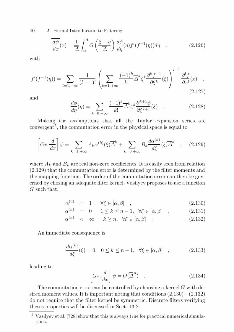
7/21/2019 Large Eddy Simulation for Incompressible Flows
http://slidepdf.com/reader/full/large-eddy-simulation-for-incompressible-flows 64/573
40 2. Formal Introduction to Filtering
dψ
dx(x) =
1
∆
βα
G
ξ − η
∆
dφ
dη(η)f (f −1(η))dη , (2.126)
with
f (f −1(η)) =
l=1,+∞
1
(l − 1)!
k=1,+∞
(−1)k
k! ∆
kζ k
∂ kf −1
∂ξ k (ξ )
l−1
∂ lf
∂xl(x) ,
(2.127)and
dφ
dη(η) =
k=0,+∞
(−1)k
k! ∆
kζ k
∂ k+1φ
∂ξ k+1 (ξ ) . (2.128)
Making the assumptions that all the Taylor expansion series areconvergent5, the commutation error in the physical space is equal to
G, d
dx
ψ =
k=1,+∞
Akα(k)(ξ )∆k
+
k=0,+∞
Bkdα(k)
dξ (ξ )∆
k, (2.129)
where Ak and Bk are real non-zero coefficients. It is easily seen from relation(2.129) that the commutation error is determined by the filter moments and
the mapping function. The order of the commutation error can then be gov-erned by chosing an adequate filter kernel. Vasilyev proposes to use a functionG such that:
α(0) = 1 ∀ξ ∈ [α, β ] , (2.130)
α(k) = 0 1 ≤ k ≤ n − 1, ∀ξ ∈ [α, β ] , (2.131)
α(k) < ∞ k ≥ n, ∀ξ ∈ [α, β ] . (2.132)
An immediate consequence is
dα(k)
dξ (ξ ) = 0, 0 ≤ k ≤ n − 1, ∀ξ ∈ [α, β ] , (2.133)
leading to G,
d
dx
ψ = O(∆
n) . (2.134)
The commutation error can be controlled by choosing a kernel G with de-sired moment values. It is important noting that conditions (2.130) – (2.132)do not require that the filter kernel be symmetric. Discrete filters verifyingtheses properties will be discussed in Sect. 13.2.
5 Vasilyev et al. [728] show that this is always true for practical numerical simula-tions.
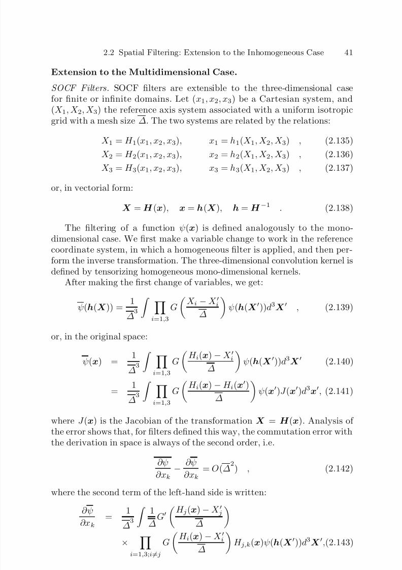
7/21/2019 Large Eddy Simulation for Incompressible Flows
http://slidepdf.com/reader/full/large-eddy-simulation-for-incompressible-flows 65/573
2.2 Spatial Filtering: Extension to the Inhomogeneous Case 41
Extension to the Multidimensional Case.
SOCF Filters. SOCF filters are extensible to the three-dimensional case
for finite or infinite domains. Let (x1, x2, x3) be a Cartesian system, and(X 1, X 2, X 3) the reference axis system associated with a uniform isotropicgrid with a mesh size ∆. The two systems are related by the relations:
X 1 = H 1(x1, x2, x3), x1 = h1(X 1, X 2, X 3) , (2.135)
X 2 = H 2(x1, x2, x3), x2 = h2(X 1, X 2, X 3) , (2.136)
X 3 = H 3(x1, x2, x3), x3 = h3(X 1, X 2, X 3) , (2.137)
or, in vectorial form:
X = H (x), x = h(X ), h = H −1 . (2.138)
The filtering of a function ψ(x) is defined analogously to the mono-dimensional case. We first make a variable change to work in the referencecoordinate system, in which a homogeneous filter is applied, and then per-form the inverse transformation. The three-dimensional convolution kernel isdefined by tensorizing homogeneous mono-dimensional kernels.
After making the first change of variables, we get:
ψ(h(X )) = 1
∆3 i=1,3
GX i − X i∆
ψ(h(X ))d3X , (2.139)
or, in the original space:
ψ(x) = 1
∆3
i=1,3
G
H i(x) − X i
∆
ψ(h(X ))d3X (2.140)
= 1
∆3 i=1,3
GH i(x) − H i(x)
∆ ψ(x)J (x)d3x, (2.141)
where J (x) is the Jacobian of the transformation X = H (x). Analysis of the error shows that, for filters defined this way, the commutation error withthe derivation in space is always of the second order, i.e.
∂ψ
∂xk− ∂ψ
∂xk= O(∆
2) , (2.142)
where the second term of the left-hand side is written:
∂ψ
∂xk=
1
∆3
1
∆G
H j(x) − X j
∆
×
i=1,3;i=j
G
H i(x) − X i
∆
H j,k(x)ψ(h(X ))d3X ,(2.143)

7/21/2019 Large Eddy Simulation for Incompressible Flows
http://slidepdf.com/reader/full/large-eddy-simulation-for-incompressible-flows 66/573
42 2. Formal Introduction to Filtering
with the notation:
H j,k(x) = ∂H j(x)
∂xk. (2.144)
Differential analysis of the commutation error is performed by consideringthe solutions of the form:
ψ(x) = ψk exp(ık · x) . (2.145)
An analogous approach to the one already made in the mono-dimensionalcase leads to the relation:
G, ∂
∂xk ψ =
−α(2)∆
2Γ kmp
∂ 2ψ
∂xm∂x p+ O(k∆)4 , (2.146)
where the function Γ kmp is defined as:
Γ kmp = hm,jq(H (x))h p,q(H (x))H j,k(x) . (2.147)
Van der Ven’s Filters. Van der Ven’s simplified filtering naturally extends tothe three-dimensional case in Cartesian coordinates by letting:
φ(x) = 1
i=1,3
δ i(x) R3 i=1,3
Gxi − xi
δ i(x) φ(x)d3x , (2.148)
in which δ i(x) is the filter cutoff length in the ith direction of space at pointx. For a kernel G verifying (2.114), the commutation error is expressed:
G, ∂
∂xj
φ = a
i=1,3
∂δ i(x)
∂xjδ i(x)n−1 ∂ nφ(x)
∂xni, (2.149)
and is formally of order n − 1.
High-Order Commuting Filters. Vasilyev’s filters are generalized to the mul-tiple dimension case in the same way as SOCF.
2.2.3 Local Spectrum of Commutation Error
A spectral tool for analyzing the wavenumber sprectrum of the commutationerror, referred to as the local spectrum analysis , was introduced by Vasilyevand Goldstein [727]. This tool enables an accurate understanding of the im-pact of the commutation error on the derivatives of the filtered quantities.Writing the convolution filter as
φ(x) = 1
∆(x)
+∞
−∞
G
x − y
∆(x)
φ(y)dy , (2.150)

7/21/2019 Large Eddy Simulation for Incompressible Flows
http://slidepdf.com/reader/full/large-eddy-simulation-for-incompressible-flows 67/573
2.3 Time Filtering: a Few Properties 43
and introducing its local Fourier decomposition (which can be evaluated usinga windowed Fourier transform on bounded domains)
φ(x) = +∞
−∞
G k∆(x) φ(k)eıkxdk , (2.151)
one can identify the coefficients of the local Fourier transform of the filteredquantity φ φ(k, x) = G k∆(x)
φ(k) . (2.152)
The commutation error can be written as
d
dx , G (φ)(x) = 1
2π +∞
−∞ 1
∆(x)
d∆(x)
dx K(k∆(x)) φ(k) eıkxdk ,
(2.153)
where the transfer function K is defined as
K(k) = −kd G(k)
dk . (2.154)
By analogy with the previous case, the local spectrum of the commutationerror is defined as
d
dx, G
(φ)(k, x) =
1
∆(x)
d∆(x)
dx K(k∆(x)) φ(k) . (2.155)
This expresion shows that the gradient of the cutoff length ∆(x) affectsthe amplitude of the commutation error, while the filter shape (more precislythe gradient of the transfer function in Fourier space) governs the spectralrepartition of the error. Analyses carried out considering convolution kernelspresented in Sect.2.1.5 reveal that the spectrum of commutation error is
global for smooth filters like the Gaussian filter (i.e. error occurs at all scales)while it is much more local for sharp filters (i.e. the commutation error isconcentrated on a narrow wavenumber range).
2.3 Time Filtering: a Few Properties
We consider here continuous causal filters of the form [603]:
φ(x, t) = G φ(x, t) = t−∞
φ(ξ, t)G(t − t)dt , (2.156)
where the kernel G satisfies immediately two of the three fundamental prop-erties given in Sect. 2.1.2, namely the linearity constraint and the constant-conservation constraint.
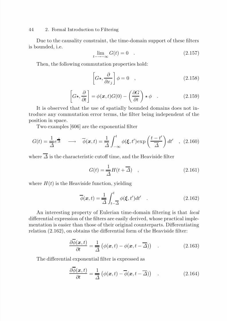
7/21/2019 Large Eddy Simulation for Incompressible Flows
http://slidepdf.com/reader/full/large-eddy-simulation-for-incompressible-flows 68/573
44 2. Formal Introduction to Filtering
Due to the causality constraint, the time-domain support of these filtersis bounded, i.e.
limt−→−∞
G(t) = 0 . (2.157)
Then, the following commutation properties hold:G,
∂
∂xj
φ = 0 , (2.158)
G,
∂
∂t
= φ(x, t)G(0) −
∂G
∂t
φ . (2.159)
It is observed that the use of spatially bounded domains does not in-
troduce any commutation error terms, the filter being independent of theposition in space.
Two examples [606] are the exponential filter
G(t) = 1
∆e t∆ −→ φ(x, t) =
1
∆
t−∞
φ(ξ, t)exp
t − t
∆
dt , (2.160)
where ∆ is the characteristic cutoff time, and the Heaviside filter
G(t) = 1∆
H (t + ∆) , (2.161)
where H (t) is the Heaviside function, yielding
φ(x, t) = 1
∆
tt−∆
φ(ξ, t)dt . (2.162)
An interesting property of Eulerian time-domain filtering is that local differential expression of the filters are easily derived, whose practical imple-
mentation is easier than those of their original counterparts. Differentiatingrelation (2.162), on obtains the differential form of the Heaviside filter:
∂φ(x, t)
∂t =
1
∆
φ(x, t) − φ(x, t − ∆)
. (2.163)
The differential exponential filter is expressed as
∂φ(x, t)
∂t =
1
∆ φ(x, t) − φ(x, t − ∆)
. (2.164)
7/21/2019 Large Eddy Simulation for Incompressible Flows
http://slidepdf.com/reader/full/large-eddy-simulation-for-incompressible-flows 69/573
3. Application to Navier–Stokes Equations
This chapter is devoted to the derivation of the constitutive equations of thelarge-eddy simulation technique, which is to say the filtered Navier–Stokes
equations. Our interest here is in the case of an incompressible viscous New-tonian fluid of uniform density and temperature.
We first describe the application of an isotropic spatial filter1 to theNavier–Stokes equations expressed in Cartesian coordinates or in general co-ordinates.
The emphasis will be put on the Eulerian, velocity–pressure formulation.2
An important point is that these two formulations lead to different commuta-tion errors with the filtering operator, and thus yield different theoretical andpractical problems. The main point is that, when curvilinear grids are con-
sidered, two possibilities arise for solving numerically the filtered governingequations:
– Conventional Approach : First the filter is applied to the Navier–Stokesequations written in Cartesian coordinates, and then the filtered equationsare transformed in general coordinates. Here, the filter is applied in thephysical space, and the filter kernels are developed within the usual Carte-sian framework (see Chap. 2).
– Alternate Approach : First the Navier–Stokes equations are expressed in
general coordinates, and then the filter is applied to the transformed equa-tions. In this case, the transformed variables are filtered using uniform filterkernels, leading to vanishing commutation errors. If physical variables arefiltered using a transformed filter kernel, some commutation errors appearand specific filters must be employed (see Chap. 2).
The differences originate from the fact that the transformation in generalcoordinates is a nonlinear operation, yielding different commutation errorsbetween the two operations.
1
Refer to the definition given in Chap. 2.2 A few works dealing with the velocity–vorticity form of the Navier–Stokes equa-tions exist [163, 485, 486]. It is important to note that the Lagrangian frameworkis employed in [485, 486]. Results dealing with large-eddy simulation within theframework of lattice-Boltzmann methods are presented in the review by Chenand Doolen [127].

7/21/2019 Large Eddy Simulation for Incompressible Flows
http://slidepdf.com/reader/full/large-eddy-simulation-for-incompressible-flows 70/573
46 3. Application to Navier–Stokes Equations
Most of the existing published works deal with the conventional approach.As a consequence, this chapter will be mostly devoted to this approach.
It should be noted that this ideal framework, which implies that the fluiddomain is unbounded, is the one nearly all authors use because it is onlyin this framework that the theory on which the subgrid modeling is basedcan be fully developed. The commutation errors between the filter and thederivation in space are then ignored. Section 3.4 is on the application of aninhomogeneous filter to the basic equations written in Cartesian coordinates.
We begin by deriving the filtered Navier–Stokes equations following theconventional approach. The various decompositions of the nonlinear term asa function of the filtered quantities are then discussed. We lastly introducethe closure problem, i.e. the representation of the unknowns as a function of
the variables in the filtered problem.
3.1 Navier–Stokes Equations
We recall here the equations governing the evolution of an incompressibleNewtonian fluid, first in the physical space, in general coordinates, and thenin the spectral space.
3.1.1 Formulation in Physical Space
In the physical space, the velocity field u = (u1, u2, u3) expressed in a refer-ence Cartesian coordinate system x = (x1, x2, x3) is a solution of the systemcomprising the momentum and continuity equations:
∂ui∂t
+ ∂
∂xj(uiuj) = − ∂p
∂xi+ ν
∂
∂xj
∂ui∂xj
+ ∂uj∂xi
, i = 1, 2, 3 , (3.1)
∂ui∂xi
= 0 , (3.2)
in which p = P/ρ and ν are, respectively, the static pressure and the as-sumedly constant, uniform kinematic viscosity. To obtain a well-posed prob-lem, we have to add initial and boundary conditions to this system.
3.1.2 Formulation in General Coordinates
The incompressible Navier–Stokes equations written in general coordinatesin strong conservation-law form [733] read:
∂
∂ξ k(J −1ξ ki ui) = 0 , (3.3)
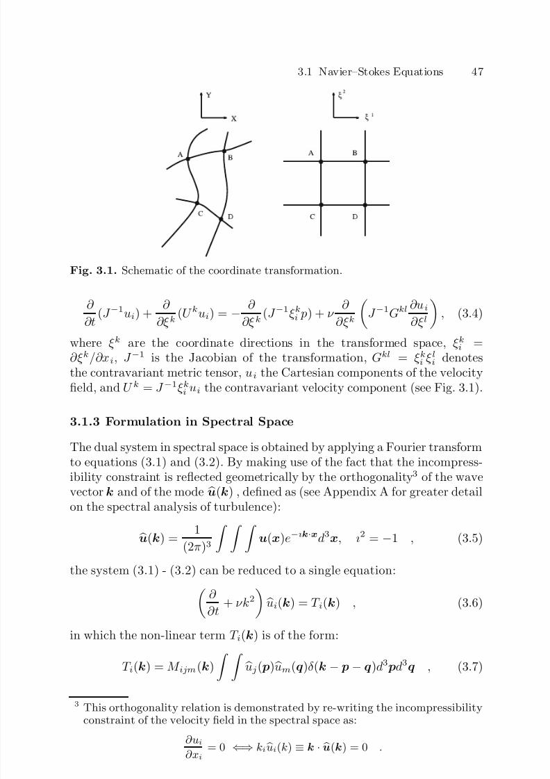
7/21/2019 Large Eddy Simulation for Incompressible Flows
http://slidepdf.com/reader/full/large-eddy-simulation-for-incompressible-flows 71/573
3.1 Navier–Stokes Equations 47
Fig. 3.1. Schematic of the coordinate transformation.
∂
∂t(J −1ui) +
∂
∂ξ k(U kui) = −
∂
∂ξ k(J −1ξ ki p) + ν
∂
∂ξ k
J −1Gkl ∂ui
∂ξ l
, (3.4)
where ξ k are the coordinate directions in the transformed space, ξ ki =∂ξ k/∂xi, J −1 is the Jacobian of the transformation, Gkl = ξ ki ξ li denotesthe contravariant metric tensor, ui the Cartesian components of the velocityfield, and U k = J −1ξ ki ui the contravariant velocity component (see Fig. 3.1).
3.1.3 Formulation in Spectral Space
The dual system in spectral space is obtained by applying a Fourier transformto equations (3.1) and (3.2). By making use of the fact that the incompress-ibility constraint is reflected geometrically by the orthogonality3 of the wavevector k and of the mode u(k) , defined as (see Appendix A for greater detailon the spectral analysis of turbulence):
u(k) = 1
(2π)3 u(x)e−ık·xd3x, ı2 = −1 , (3.5)
the system (3.1) - (3.2) can be reduced to a single equation: ∂
∂t + νk2
ui(k) = T i(k) , (3.6)
in which the non-linear term T i(k) is of the form:
T i(k) = M ijm(k)
uj( p)
um(q)δ (k − p− q)d3 pd3q , (3.7)
3 This orthogonality relation is demonstrated by re-writing the incompressibilityconstraint of the velocity field in the spectral space as:
∂ui∂xi
= 0 ⇐⇒ ki ui(k) ≡ k · u(k) = 0 .

7/21/2019 Large Eddy Simulation for Incompressible Flows
http://slidepdf.com/reader/full/large-eddy-simulation-for-incompressible-flows 72/573
48 3. Application to Navier–Stokes Equations
with:M ijm(k) = − ı
2 (kmP ij(k) + kjP im(k)) , (3.8)
in which δ is the Kronecker symbol and P ij(k) is the projection operator onthe plane orthogonal to the vector k. This operator is written:
P ij(k) =
δ ij − kikj
k2
. (3.9)
3.2 Filtered Navier–Stokes Equations in Cartesian
Coordinates (Homogeneous Case)This section describes the equations of large-eddy simulation such as theyare obtained by applying a homogeneous filter verifying the properties of linearity, conservation of constants, and commutation with derivation, to theNavier–Stokes equations. These are the equations that will be resolved in thenumerical simulation.
3.2.1 Formulation in Physical Space
In light of the commutation with derivation property, the application of a fil-ter to equations (3.1) and (3.2) is expressed:
∂ui∂t
+ ∂
∂xj(uiuj) = − ∂p
∂xi+ ν
∂
∂xj
∂ui∂xj
+ ∂uj∂xi
, (3.10)
∂ui∂xi
= 0 , (3.11)
where p is the filtered pressure. The filtered momentum equation brings outthe non-linear term uiuj which, in order for this equation to be usable, willhave to be expressed as a function of u and u, which are now the onlyunknowns left in the problem and where:
u = u − u . (3.12)
This decomposition is not unique, and will be discussed in the followingsection.
3.2.2 Formulation in Spectral Space
Using the equivalence ui(k) = G(k) ui(k), the momentum equation in thespectral space obtained by multiplying equation (3.6) by the transfer function

7/21/2019 Large Eddy Simulation for Incompressible Flows
http://slidepdf.com/reader/full/large-eddy-simulation-for-incompressible-flows 73/573
3.3 Decomposition of the Non-linear Term. Conventional Approach 49
G(k) is expressed:
∂
∂t + 2νk2 G(k) ui(k) = G(k)T i(k) , (3.13)
in which the filtered non-linear term G(k)T i(k) is written:
G(k)T i(k) = M ijm(k)
G(k) uj( p) um(q)δ (k − p − q)d3 pd3q . (3.14)
The filtered non-linear term (3.14) brings out the contributions of themodes
u( p) and
u(q). To complete the decomposition, these modes also
have to be expressed as the sum of a filtered part and a fluctuation. This isthe same problem as the one encountered when writing the equations in thephysical space. This operation is described in the following section.
3.3 Decomposition of the Non-linear Term.Associated Equations for the Conventional Approach
This section details the various existing decompositions of the non-linear term
and the associated equations written in Cartesian coordinates.
3.3.1 Leonard’s Decomposition
Expression in Physical Space. Leonard [436] expresses the non-linearterm in the form of a triple summation:
uiuj = (ui + ui)(uj + uj) (3.15)
= uiuj + uiuj + ujui + uiuj . (3.16)
The non-linear term is now written entirely as a function of the filteredquantity u and the fluctuation u. We then have two versions of this [762].
The first considers that all the terms appearing in the evolution equationsof a filtered quantity must themselves be filtered quantities, because the sim-ulation solution has to be the same for all the terms. The filtered momentumequation is then expressed:
∂ui
∂t
+ ∂
∂xj uiuj =
− ∂ p
∂xi+ ν
∂
∂xj ∂ui
∂xj+
∂uj
∂xi− ∂τ ij
∂xj, (3.17)
in which the subgrid tensor τ , grouping together all the terms that are notexclusively dependent on the large scales, is defined as:
τ ij = C ij + Rij = uiuj − uiuj , (3.18)
7/21/2019 Large Eddy Simulation for Incompressible Flows
http://slidepdf.com/reader/full/large-eddy-simulation-for-incompressible-flows 74/573
50 3. Application to Navier–Stokes Equations
where the cross-stress tensor, C , which represents the interactions betweenlarge and small scales, and the Reynolds subgrid tensor, R, which reflects theinteractions between subgrid scales, are expressed:
C ij = uiuj + ujui , (3.19)
Rij = uiuj . (3.20)
In the following, this decomposition will be called double decomposition.The other point of view consists of considering that it must be possible
to evaluate the terms directly from the filtered variables. But the uiuj termcannot be calculated directly because it requires a second application of thefilter. To remedy this, Leonard proposes a further decomposition:
uiuj =
uiuj − uiuj
+ uiuj
= Lij + uiuj . (3.21)
The new L term, called Leonard tensor, represents interactions among thelarge scales. Using this new decomposition, the filtered momentum equationbecomes:
∂ui
∂t
+ ∂
∂xj
(uiuj) =
−
∂ p
∂xi
+ ν ∂
∂xj ∂ui
∂xj
+ ∂uj
∂xi −
∂τ ij
∂xj
. (3.22)
The subgrid tensor τ , which now groups all the terms that are not ex-pressed directly from u, takes the form:
τ ij = Lij + C ij + Rij = uiuj − uiuj . (3.23)
This decomposition will be designated hereafter the Leonard or tripledecomposition. Equation (3.22) and the subgrid term τ ij defined by (3.23)can be obtained directly from the Navier–Stokes equations without using the
Leonard decomposition for this. It should be noted that the term uiuj isa quadratic term and that it contains frequencies that are in theory higherthan each of the terms composing. So in order to represent it completely,more degrees of freedom are needed than for each of the terms ui and uj
4.We may point out that, if the filter is a Reynolds operator, then the
tensors C ij and Lij are identically zero5 and the two decompositions arethen equivalent, since the subgrid tensor is reduced to the tensor Rij.
4 In practice, if the large-eddy simulation filter is associated with a given compu-tational grid on which the Navier–Stokes equations are resolved, this means that
the grid used for composing the uiuj product has to be twice as fine (in eachdirection of space) as the one used to represent the velocity field. If the productis composed on the same grid, then only the uiuj term can be calculated.
5 It is recalled that if the filter is a Reynolds operator, then we have the threefollowing properties (see Appendix A):
u = u, u = 0, uu = u u ,
7/21/2019 Large Eddy Simulation for Incompressible Flows
http://slidepdf.com/reader/full/large-eddy-simulation-for-incompressible-flows 75/573
3.3 Decomposition of the Non-linear Term. Conventional Approach 51
Writing the Navier–Stokes equations (3.1) in the symbolic form
∂ u
∂t + NS (u) = 0 , (3.24)
the filtered Navier–Stokes equations are expressed
G ∂ u
∂t =
∂ u
∂t = −G NS (u) (3.25)
= −NS (u) − [G, NS ](u) , (3.26)
where [., .] is the commutator operator introduced in Sect. 2.1.2. We notethat the subgrid tensor corresponds to the commutation error between the
filter and the non-linear term. Introducing the bilinear form B(·, ·):
B(ui, uj) ≡ uiuj , (3.27)
we getτ ij = [G, B](ui, uj) . (3.28)
Double decomposition (3.18) leads to the following equation for the re-solved kinetic energy q 2r = uiui/2:
∂q 2r∂t
= uiuj ∂ui∂xj I
+ τ ij ∂ui∂xj II
− ν ∂ui∂xj
∂ui∂xj
III
− ∂
∂xi(ui p) IV
+ ∂
∂xi
ν
∂q 2r∂xi
V
− ∂
∂xj uiuiuj
V I
− ∂
∂xj(uiτ ij)
V II
. (3.29)
This equation shows the existence of several mechanisms exchanging ki-netic energy at the resolved scales:
whence
C ij = uiuj + ujui
= uiuj + ujui
= 0 ,
Lij = uiuj − uiuj
= uiuj − uiuj
= 0 .
.

7/21/2019 Large Eddy Simulation for Incompressible Flows
http://slidepdf.com/reader/full/large-eddy-simulation-for-incompressible-flows 76/573
52 3. Application to Navier–Stokes Equations
– I - production– II - subgrid dissipation– III - dissipation by viscous effects– IV - diffusion by pressure effect– V - diffusion by viscous effects– V I - diffusion by interaction among resolved scales– V II - diffusion by interaction with subgrid modes.
Leonard’s decomposition (3.23) can be used to obtain the similar form:
∂q 2r∂t
= − ∂q 2r uj∂xj VIII
+ τ ij∂ui∂xj IX
− ν ∂ui∂xj
∂ui∂xj X
− ∂
∂xi(ui p) XI
+ ∂
∂xi
ν
∂q 2r∂xi
XII
+ uiuj∂ui∂xj
XIII
− ∂
∂xj(uiτ ij)
XIV
. (3.30)
This equation differs from the previous one only in the first and sixthterms of the right-hand side, and in the definition of tensor τ :
– V I II - advection– IX - idem II – X - idem III – XI - idem IV – XII - idem V – XIII - production– XIV - idem V II
The momentum equation for the small scales is obtained by subtract-ing the large scale equation from the unfiltered momentum equation (3.1),making, for the double decomposition:
∂ui∂t
+ ∂
∂xj
(ui + ui)(uj + uj) − uiuj
= − ∂p
∂xi+
∂τ ij∂xi
+ ν ∂
∂xj
∂ui∂xj
+∂uj∂xi
, (3.31)
and, for the triple decomposition:∂ui∂t
+ ∂
∂xj
(ui + ui)(uj + uj) − uiuj
= − ∂p
∂xi+
∂τ ij∂xi
+ ν ∂
∂xj
∂ui∂xj
+∂uj∂xi
. (3.32)

7/21/2019 Large Eddy Simulation for Incompressible Flows
http://slidepdf.com/reader/full/large-eddy-simulation-for-incompressible-flows 77/573
3.3 Decomposition of the Non-linear Term. Conventional Approach 53
The filtered subgrid kinetic energy q 2sgs = ukuk/2 equation obtained bymultiplying (3.32) by ui and filtering the relation thus derived is expressed:
∂q 2sgs
∂t = − ∂
∂xj
q 2sgsuj
XV
− 1
2
∂
∂xj(uiuiuj − ujuiui)
XV I
− ∂
∂xj( puj − p uj) XVII
+ ∂
∂xj
ν
∂q 2sgs
∂xj
XVIII
+ ∂
∂xj(τ ijui) XIX
− ν ∂ui
∂xj
∂ui
∂xj − ∂ui
∂xj
∂ui
∂xj XX
−τ ij
∂ui
∂xj XXI
. (3.33)
– XV - advection– XV I - turbulent transport– X V I I - diffusion by pressure effects– X V I II - diffusion by viscous effects– XIX - diffusion by subgrid modes
– XX - dissipation by viscous effects– XXI - subgrid dissipation.
For the double decomposition, equation (3.31) leads to:
∂q 2sgs
∂t = − ∂
∂xj
uiuiuj − uiuiuj
XXII
+ uiuj∂ui∂xj
− uiuj∂ui∂xj
XXIII
− ∂
∂xj puj − p uj XXIV
+ ν ui∂ 2ui
∂x2j − ui
∂ 2ui
∂x2j
XXV
+ ∂
∂xj
τ ijui
− τ ij∂ui∂xj
XXVI
, (3.34)
with:
– XXII - turbulent transport– XXIII - production– XXIV - diffusion by pressure effects– XXV - viscous effects– X XV I - subgrid dissipation and diffusion

7/21/2019 Large Eddy Simulation for Incompressible Flows
http://slidepdf.com/reader/full/large-eddy-simulation-for-incompressible-flows 78/573
54 3. Application to Navier–Stokes Equations
It is recalled that, if the filter used is not positive, the generalized subgridkinetic energy q 2gsgs defined as the half-trace of the subgrid tensor,
q 2gsgs = τ kk/2 = 12
uiui + uiui ,
can admit negative values locally (see Sect. 3.3.5). If the filter is a Reynoldsoperator, the subgrid tensor is then reduced to the subgrid Reynolds tensorand the generalized subgrid kinetic energy is equal to the subgrid kineticenergy, i.e.
q 2sgs ≡ 1
2uiu
i = q 2gsgs ≡ τ kk/2 . (3.35)
Expression in Spectral Space. Both versions of the Leonard decompo-
sition can be transcribed in the spectral space. Using the definition of thefluctuation u(k) as ui(k) = (1 − G(k)) ui(k) , (3.36)
the filtered non-linear term G(k)T i(k) is expressed, for the triple decompo-sition:
G(k)T i(k) = M ijm(k)
G( p)
G(q)
uj( p)
um(q)δ (k − p − q)d3 pd3q
− M ijm(k) (1 − G(k)) G( p) G(q)
× uj( p) um(q)δ (k − p − q)d3 pd3q
+ M ijm(k)
G(k) G( p)(1 − G(q)) + G(q)(1 − G( p))
× uj( p) um(q)δ (k − p − q)d3 pd3q
+ M ijm(k)
G(k)
(1 −
G(q))(1 −
G( p))
× uj( p) um(q)δ (k − p − q)d3 pd3q . (3.37)
The first term of the right-hand side corresponds to the contribution uiuj ,the second to the Leonard tensor L, the third to the cross stresses representedby the tensor C , and the fourth to the subgrid Reynolds tensor R. This isillustrated by Fig. 3.2.
The double decomposition is derived by combination of the first two termsof the right-hand side of (3.37):
G(k)T i(k) = M ijm(k) G( p) G(q) G(k)
× uj( p) um(q)δ (k − p − q)d3 pd3q

7/21/2019 Large Eddy Simulation for Incompressible Flows
http://slidepdf.com/reader/full/large-eddy-simulation-for-incompressible-flows 79/573
3.3 Decomposition of the Non-linear Term. Conventional Approach 55
Fig. 3.2. Representation of the various Leonard decomposition terms in the spec-
tral space, when using a sharp cutoff filter with a cutoff frequency kc.
+ M ijm(k)
G(k) G( p)(1 − G(q)) + G(q)(1 − G( p))
× uj( p) um(q)δ (k − p − q)d3 pd3q
+ M ijm(k) G(k)(1 − G(q))(1 − G( p))× uj( p) um(q)δ (k − p − q)d3 pd3q . (3.38)
The first term of the right-hand side corresponds to the contribution uiujin the physical space, and the last two remain unchanged with respect to thetriple decomposition. Let us note that the sum of the contributions of thecross tensor and the subgrid Reynolds tensor simplifies to the form:
C ij + Rij = M ijm(k) (1
− G( p) G(q)) G(k)
× uj( p) um(q)δ (k − p − q)d3 pd3q . (3.39)
The momentum equations corresponding to these two decompositions arefound by replacing the right-hand side of equation (3.13) with the desiredterms. For the double decomposition, we get:

7/21/2019 Large Eddy Simulation for Incompressible Flows
http://slidepdf.com/reader/full/large-eddy-simulation-for-incompressible-flows 80/573
56 3. Application to Navier–Stokes Equations
∂
∂t
+ νk2 G(k) ui(k) = M ijm(k) G( p) G(q) G(k)
× uj( p) um(q)δ (k − p − q)d3 pd3q
+ M ijm(k)
(1 − G( p) G(q)) G(k)
× uj( p) um(q)δ (k − p − q)d3 pd3q ,
(3.40)
and for the triple decomposition:
∂
∂t + νk2 G(k) ui(k) = M ijm(k) G( p) G(q)
× uj( p) um(q)δ (k − p − q)d3 pd3q
− M ijm(k)
(1 − G(k)) G( p) G(q)
× uj( p) um(q)δ (k − p − q)d3 pd3q
+ M ijm(k)
G(k)
G( p)(1 −
G(q))
+ G(q)(1 − G( p))× uj( p) um(q)δ (k − p − q)d3 pd3q
+ M ijm(k)
G(k)
(1 − G(q))(1 − G( p))
× uj( p) um(q)δ (k − p − q)d3 pd3q . (3.41)
For both decompositions, the momentum equation can be expressed inthe symbolic form:
∂ ∂t
+ νk2 G(k) ui(k) = T r(k) + T sgs(k) , (3.42)
in which T r(k) designates the transfer terms calculated directly from theresolved modes, and is therefore equivalent to the contribution of the uiujterm in the case of the triple decomposition, and that of the uiuj term forthe double decomposition. The T sgs(k) term designates the other non-linearterms, and therefore corresponds to the contribution of the subsidiary termsuch as defined above. Let E (k) be the energy contained on the sphere of radius k. It is calculated as:
E (k) = 12
k2 u(k) · u∗(k)dS (k) , (3.43)
where dS (k) is the surface element of the sphere, and where the asterisk desig-nates a conjugate complex number. The kinetic energy of the resolved modescontained on this same sphere, denoted E r(k), is defined by the relation

7/21/2019 Large Eddy Simulation for Incompressible Flows
http://slidepdf.com/reader/full/large-eddy-simulation-for-incompressible-flows 81/573
3.3 Decomposition of the Non-linear Term. Conventional Approach 57
E r(k) = 1
2k2
G(k)
u(k) ·
G(k)
u∗(k)dS (k) (3.44)
= G2
(k)E (k) . (3.45)
We return to the kinetic energy of the resolved modes, q 2r = uiui/2, bysummation on all the wave numbers:
q 2r =
∞0
E r(k)dk . (3.46)
It is important to note that E r(k) is related to the energy of the resolvedmodes, which is generally not equal to the filtered part of the kinetic energy
which, for its part, is associated with the quantity denoted E (k), defined as
E (k) = G(k)E (k) . (3.47)
The identity of these two quantities is verified when the transfer func-tion is such that G2(k) = G(k), ∀k, i.e. when the filter used is a projector.The evolution equation for E r(k) is obtained by multiplying the filtered mo-
mentum equation (3.13) by k2
G(k)
u∗(k), and then integrating the result on
the sphere of radius k. Using the double decomposition we get the followingequation:
∂
∂t + 2νk2
E r(k) =
1
2
∆
G( p) G(q) G2(k)S (k| p, q)d pdq
+ 1
2
∆
(1 − G( p) G(q)) G2(k)S (k| p, q)d pdq ,
(3.48)
and the triple decomposition:
∂
∂t + 2νk2E r(k) =
1
2
∆
G( p) G(q) G(k)S (k| p, q)d pdq
− 1
2
G(k)(1 − G(k)) G( p) G(q)S (k| p, q)d pdq
+ 1
2
∆
G2(k) G( p)
× (1 − G(q)) +
G(q)(1 −
G( p))
S (k| p, q)d pdq
+ 1
2
∆
G2(k)
(1 − G(q))(1 − G( p))
×S (k| p, q)d pdq , (3.49)
in which

7/21/2019 Large Eddy Simulation for Incompressible Flows
http://slidepdf.com/reader/full/large-eddy-simulation-for-incompressible-flows 82/573
58 3. Application to Navier–Stokes Equations
S (k| p, q) = 16π2kpqM ijm(k)
uj( p)
um(q)
ui(−k)δ (k − p − q) , (3.50)
and where the symbol ∆ designates integration over the interval
|k − p| < q < k + p.Following the example of what was done for the momentum equations,
the kinetic energy evolution equation for the resolved modes can be expressedin the abbreviated form
∂
∂t + 2νk2
E r(k) = T er (k) + T esgs(k) . (3.51)
The terms T er (k) and T esgs(k) represent, respectively, the energy transfers
of mode k
with all the other modes associated with the terms that can becalculated directly from the resolved modes, and the subgrid terms.The ki-netic energy conservation property for inviscid fluids, i.e. in the case of zeroviscosity, implies:
(T er (k) + T esgs(k))d3k = 0 . (3.52)
The momentum equations for the unresolved scales are obtained by alge-braic manipulations strictly analogous to those used for obtaining the equa-tions for the resolved scales, except that this time equation (3.6) is multiplied
by (1 − G(k)) instead of G(k). These equations are written:∂
∂t + νk2
(1 − G(k)) ui(k) = (1 − G(k))T i(k) . (3.53)
Calculations similar to those explained above lead to:∂
∂t + νk2
ui(k) = M ijm(k)
G( p)
G(q)(1 −
G(k))
× uj( p) um(q)δ (k − p − q)d
3
pd
3
q
+ M ijm(k)
(1 − G(k))
G( p)(1 − G(q))
+ G(q)(1 − G( p))
× uj( p) um(q)δ (k − p − q)d3 pd3q
+ M ijm(k)
(1 −
G(k))
(1 −
G(q))(1 −
G( p))
× uj( p) um(q)δ (k − p − q)d3 pd3q . (3.54)
The first term of the right-hand side represents the contribution of theinteractions between large scale modes, the second the contribution of thecross interactions, and the last the interactions among the subgrid modes.
7/21/2019 Large Eddy Simulation for Incompressible Flows
http://slidepdf.com/reader/full/large-eddy-simulation-for-incompressible-flows 83/573
3.3 Decomposition of the Non-linear Term. Conventional Approach 59
Let E sgs be the energy contained in the subgrid modes. This energy isdefined as:
E sgs(k) = 12
k2 (1 − G(k)) u(k) · (1 − G(k)) u∗(k)dS (k) (3.55)
= (1 − G)2(k)E (k) , (3.56)
and is different, in the general case, from the kinetic energy fluctuationE (k) = (1 − G)(k)E (k), though the equality of these two quantities is ver-ified when the filter is a Reynolds operator. Simple calculations give us thefollowing evolution equation for E sgs(k):
∂
∂t + 2νk2E sgs(k) =
1
2 ∆ G( p) G(q)(1 − G(k))2
S (k| p, q)d pdq
+ 1
2
∆
(1 − G(k)) G( p)(1 − G(q))
+ G(q)(1 − G( p))
S (k| p, q)d pdq
+ 1
2
∆
(1 − G(k))2(1 − G(q))(1 − G( p))
×S (k| p, q)d pdq , (3.57)
where the notation used is the same as for the kinetic energy evolution equa-tion of the resolved modes. The subgrid kinetic energy q 2sgs is obtained bysummation over the entire spectrum:
q 2sgs =
∞0
E sgs(k)dk . (3.58)
3.3.2 Germano Consistent Decomposition
This section presents the Germano consistent decomposition, which is a gen-
eralization of the Leonard decomposition.
Definition and Properties of Generalized Central Moments. For con-venience, we use [φ]G to denote the resolved part of the field φ, defined as inthe first chapter, where G is the convolution kernel, i.e.:
[φ]G(x) ≡ G φ(x) ≡ +∞
−∞
G(x − ξ)φ(ξ)d3ξ . (3.59)
We define the generalized central moments with the filter G, denoted τ G,as [244, 246, 247, 248]:
τ G(φ1, φ2) = [φ1φ2]G − [φ1]G[φ2]G , (3.60)
τ G(φ1, φ2, φ3) = [φ1φ2φ3]G − [φ1]Gτ G(φ2, φ3) − [φ2]Gτ G(φ1, φ3)
−[φ3]Gτ G(φ1, φ2) − [φ1]G[φ2]G[φ3]G , (3.61)
τ G(φ1, φ2, φ3, φ4) = ... (3.62)

7/21/2019 Large Eddy Simulation for Incompressible Flows
http://slidepdf.com/reader/full/large-eddy-simulation-for-incompressible-flows 84/573
60 3. Application to Navier–Stokes Equations
The generalized central moments thus defined verify the following prop-erties:
τ G(φ, ψ) = τ G(ψ, φ) , (3.63)τ G(φ, a) = 0, for a = const. , (3.64)
τ G(φ,ψ,a) = 0, for a = const. , (3.65)
∂τ G(φ, ψ)/∂s = τ G(∂φ/∂s,ψ) + τ G(φ,∂ψ/∂s), s = x, t . (3.66)
If we perform the decomposition φ = φ1 + φ2, ψ = ψ1 + ψ2, we get:
τ G(ψ1 + ψ2, φ1 + φ2) = τ G(ψ1, φ1) + τ G(ψ1, φ2)
+ τ G(ψ2, φ1) + τ G(ψ2, φ2) . (3.67)
The generalized central moments also appear as the coefficients of thefollowing formal Taylor expansion [247]:
[φ(a1,...,an)]G = φ([a1]G, ..., [an]G) +l,m
τ G(al, am)
2! ylm
+l,m,k
τ G(al, am, ak)
3! ylmk + ... , (3.68)
with
ylm = ∂ 2φ([a1]G, ..., [an]G)
∂ [al]G∂ [am]G, ylmk =
∂ 3φ([a1]G, ..., [an]G)
∂ [al]G∂ [am]G∂ [ak]G,
and where the ai are generic turbulent quantities. The relation (3.68) estab-lishes a link between the filtered value of the functional φ and its unfilteredcounterpart applied to the filtered variables [ai]G.
Consistent Decomposition: Associated Equations. By applying theproperty (3.67) to the decomposition φ = [φ]G + φ, ψ = [ψ]G + ψ, we get:
τ G([φ]G + φ, [ψ]G + ψ) = τ G([φ]G, [ψ]G) + τ G(φ, [ψ]G)
+τ G([φ]G, ψ) + τ G(φ, ψ) . (3.69)
This decomposition is said to be consistent because it is consistent withthe definition of the generalized central moments, ensuring that all the termsin it are of the same form, which is not true of the Leonard decomposition.The various terms of the right-hand side of equation (3.69) can be interpretedas generalizations of the terms of the Leonard triple decomposition. By ap-
plying this definition to the components of the velocity fields, the subgridtensor (3.23) appears in a double form:
τ G(ui, uj) = [uiuj ]G − [ui]G[uj]G
= Lij + C ij + Rij
= Lij + Cij + Rij , (3.70)
7/21/2019 Large Eddy Simulation for Incompressible Flows
http://slidepdf.com/reader/full/large-eddy-simulation-for-incompressible-flows 85/573
3.3 Decomposition of the Non-linear Term. Conventional Approach 61
in which the tensors L, C and R are defined as:
Lij = τ G([ui]G, [uj]G) , (3.71)
Cij = τ G([ui]G, uj) + τ G(ui, [uj]G) , (3.72)
Rij = τ G(ui, uj) , (3.73)
and represent, respectively, the interactions between the large scales, thecross interactions, and the interactions among subgrid scales. They thereforerepresent tensors defined by Leonard, but are not the same as them in thegeneral case.
By bringing out the generalized central moments, the filtered momentumequations are written in the form:
∂ [ui]G
∂t +
∂
∂xj([ui]G[uj]G) = −∂ [ p]G
∂xi+ ν
∂
∂xj
∂ [ui]G
∂xj+
∂ [uj]G
∂xi
−∂τ G(ui, uj)
∂xj. (3.74)
This equation is equivalent to the one derived from the triple Leonarddecomposition. Similarly, the subgrid kinetic energy evolution equation (3.33)is re-written as:
∂q 2sgs
∂t =
∂
∂xj
1
2τ G(ui, ui, uj) + τ G( p, uj) − ν
∂q 2sgs
∂xj
− ντ G(∂ui/∂xj , ∂ui/∂xj) − τ G(ui, uj)∂ [ui]G
∂xj. (3.75)
It is easy to check that the structure of the filtered equations is, in terms
of generalized central moments, independent of the filter used. This is calledthe filtering (or averaging) invariance property .
3.3.3 Germano Identity
Basic Germano Identity. Subgrid tensors corresponding to two differentfiltering levels can be related by an exact relation derived by Germano [246].
A sequential application of two filters, F and G, is denoted:
[ui]FG = [[ui]F]G = [[ui]G]F , (3.76)
or equivalently:
[ui]FG(x) =
+∞
−∞
G(x − y)d3y
+∞
−∞
F (y − ξ)ui(ξ)d3ξ . (3.77)

7/21/2019 Large Eddy Simulation for Incompressible Flows
http://slidepdf.com/reader/full/large-eddy-simulation-for-incompressible-flows 86/573
62 3. Application to Navier–Stokes Equations
Fig. 3.3. Illustration of the two filtering levels, F and G, involved in the Germanoidentity. Associated cutoff wave numbers are denoted kF and kG, respectively. Re-solved velocity fields are uF and uG, and the associated subgrid tensors are τ F andτ G, respectively.
Here, [ui]FG
corresponds to the resolved field for the double filtering F G.The two filtering levels are illustrated in Fig. 3.3.
The subgrid tensor associated with the level F G is defined as the followinggeneralized central moment:
τ FG(ui, uj) = [uiuj ]FG − [ui]FG[uj]FG . (3.78)
This expression is a trivial extension of the definition of the subgrid ten-sor associated with the G filtering level. By definition, the subgrid tensorτ G([ui]F, [uj]F) calculated from the scales resolved for the F filtering level, is
written: τ G([ui]F, [uj]F) = [[ui]F[uj ]F]G − [ui]FG[uj ]FG . (3.79)
These two subgrid tensors are related by the following exact relation,called the Germano identity:
τ FG(ui, uj) = [τ F(ui, uj)]G + τ G([ui]F, [uj ]F) . (3.80)
This relation can be interpreted physically as follows. The subgrid tensorat the F G filtering level is equal to the sum of the subgrid tensor at the F level filtered at the G level and the subgrid tensor at the G level calculated
from the field resolved at the F level. This relation is local in space and timeand is independent of the filter used.
It is interesting noting that re-writing the subgrid tensor as
τ FG(ui, uj) = [F G, B](ui, uj) ,
7/21/2019 Large Eddy Simulation for Incompressible Flows
http://slidepdf.com/reader/full/large-eddy-simulation-for-incompressible-flows 87/573
3.3 Decomposition of the Non-linear Term. Conventional Approach 63
where [., .] is the commutator operator (see equation (2.13)) and B(., .) thebilinear form defined by relation (3.27), the Germano identity (3.80) is strictlyequivalent to relation (2.16):
[F G, B](ui, uj) = [F , B] (G)(ui, uj) + (F ) [G,B](ui, uj). (3.81)
The previous Germano identity can be referred to as the multiplicative Germano identity [251], because it is based on a sequential application of the two filters. An additive Germano identity can also be defined consideringthat the second filtering level is defined by the operator (F + G) and not bythe operator (G) (F ). The equivalent relation for (3.80) is
τ F+G(ui, uj) = τ F(ui, uj) + τ G(ui, uj)
−([ui]F[uj ]G + [ui]G[uj]F) . (3.82)
Multilevel Germano Identity. The Multiplicative Germano Identity canbe extended to the case of N filtering levels, Gi, i = 1, N , with associatedcharacteristic lengths ∆1 ≤ ∆2 ≤ ... ≤ ∆N [248, 710, 633].
We define the nth level filtered variable φn
as
φn
= Gn Gn−1 ... G1 φ = Gn1 φ , (3.83)
with
Gn
m ≡Gn Gn−1 ... Gm,
Gn
n
= I d, ∀
m∈
[1, n] . (3.84)
Let τ nij = uiujn−uni u
nj be the subgrid tensor associated to the nth filtering
level. The classical two-level Germano identity (3.80) reads
τ n+1ij = τ nij
n+1+ Ln+1
ij , Ln+1ij = uni u
nj
n+1 − un+1i un+1
j . (3.85)
Simple algebraic developments lead to the following relation between twofiltering levels n and m, with m < n:
τ nij = Lnij + k=m+1,n−1 Gnk+1Lkij +
Gnm+1τ mij , (3.86)
resulting in a fully general mutilevel identity.
Generalized Germano Identity. A more general multiplicative iden-tity is obtained by applying an arbitrary operator L to the basic iden-tity (3.81) [629], yielding
L[F G, B](ui, uj)] = L[F , B] (G)(ui, uj)
+ (F ) [G,B](ui, uj) . (3.87)
For linear operators, we get
L[F G, B](ui, uj)] = L[F , B] (G)(ui, uj)+ L(F ) [G,B](ui, uj) . (3.88)
Application to the multilevel identity (3.86) is straightforward.
7/21/2019 Large Eddy Simulation for Incompressible Flows
http://slidepdf.com/reader/full/large-eddy-simulation-for-incompressible-flows 88/573
64 3. Application to Navier–Stokes Equations
3.3.4 Invariance Properties
One of the basic principles of modeling in mechanics is to conserve the generic
properties of the starting equations [681, 230, 260, 572, 326, 398].We consider in the present section the analysis of some invariance/symme-
try properties of the filtered Navier–Stokes equations, and the resulting con-straints for subgrid models. It is remembered that a differential equation willbe said to be invariant under a transformation if it is left unchanged by thistransformation. It is important to note that these properties are not sharedby the boundary conditions. It is shown that properties of the filtered Navier–Stokes equations depend on the filter used to operate the scale separation.The preservation of the symmetry properties of the original Navier–Stokes
equations will then lead to the definition of specific requirements for the filterkernel6 G(x, ξ ). The properties considered below are:
– Galilean invariance for the spatial filtering approach (p. 64).– Galilean invariance for the time-domain filtering approach (p. 66).– General frame-invariance properties for the time-domain filtering approach
(p. 67).– Time invariance for the spatial filtering approach (p. 69).– Rotation invariance for the spatial filtering approach (p. 70).– Reflection invariance for the spatial filtering approach (p. 70).
– Asymptotic Material Frame Indifference for the spatial filtering approach(p. 71).
Galilean Invariance for Spatial filter. This section is devoted to the anal-ysis by Speziale [681] of the preservation of the Galilean invariance propertyfor translations of the Navier–Stokes equations, first by applying a spatialfilter, then by using the different decompositions presented above.
Let us take the Galilean transformation (translation):
x• = x + V t + b, t• = t , (3.89)
in which V and b are arbitrary uniform vectors in space and constant in time.If the (x, t) frame of reference is associated with an inertial frame, then sois (x•, t•). Let u and u• be the velocity vectors expressed in the base frameof reference and the new translated one, respectively. The passage from onesystem to the other is defined by the relations:
u• = u + V , (3.90)
∂
∂x•i=
∂
∂xi, (3.91)
∂
∂t• =
∂
∂t − V i
∂
∂xi. (3.92)
6 We will only consider filters with constant and uniform cutoff length, i.e. ∆ isindependent on both space and time. Variable length filters are anisotropic ornonhomogeneous, and violate the following properties in the most general case.

7/21/2019 Large Eddy Simulation for Incompressible Flows
http://slidepdf.com/reader/full/large-eddy-simulation-for-incompressible-flows 89/573
3.3 Decomposition of the Non-linear Term. Conventional Approach 65
The proof of the invariance of the Navier–Stokes equations for the trans-formation (3.89) is trivial and is not reproduced here. With this property inhand, what remains to be shown in order to prove the invariance of the filteredequations by such a transformation is that the filtering process preserves thisproperty.
Let there be a variable φ such that
φ• = φ . (3.93)
The filtering in the translated frame of reference is expressed:
φ•
=
G(x• − x•)φ•(x•)d3x•
. (3.94)
By using the previous relations, we get:
x• − x• = (x + V t + b) − (x + V t + b) = x − x , (3.95)
d3x•
=
∂x•i∂xj
d3x = d3x , (3.96)
and thus, by substitution, the equality:
φ• = G(x − x)φ(x)d3x = φ , (3.97)
which completes the proof 7. The invariance of the Navier–Stokes equationsfor the transformation (3.89) implies that the sum of the subgrid terms andthe convection term, calculated directly from the large scales, is also invariant,but not that each term taken individually is invariant. In the following, westudy the properties of each term arising from the Leonard and Germanodecompositions.
The above relations imply:
u• = u + V , u• = u, u• = u , (3.98)
which reflects the fact that the velocity fluctuations are invariant by Galileantransformation, while the total velocity is not. In the spectral space, thiscorresponds to the fact that only the constant mode does not remain invariantby this type of transformation since, with the V field being uniform, it aloneis affected by the change of coordinate system8.
7 A sufficient condition is that the filter kernel appears as a function of x − x.8
This is expressed: V = cste =⇒ V (k) = 0 ∀k = 0 ,
and thus u•(k) = u(k) ∀k = 0 , u•(0) = u(0) + V (0) .
7/21/2019 Large Eddy Simulation for Incompressible Flows
http://slidepdf.com/reader/full/large-eddy-simulation-for-incompressible-flows 90/573
66 3. Application to Navier–Stokes Equations
In the translated frame, the Leonard tensor takes the form:
L•
ij
= u•
i
u•
j −u•
i
u•
j
(3.99)
= Lij +
V iuj + V jui− (V iuj + V jui) (3.100)
= Lij −
V iuj + V jui
. (3.101)
So this tensor is not invariant. Similar analyses show that:
C •ij = C ij +
V iuj + V jui
, (3.102)
R•ij = Rij , (3.103)
L•ij + C •ij = Lij + C ij . (3.104)
The tensor C is thus not invariant in the general case, while the tensor Rand the groups L+C and L+C +R are. A difference can be seen to appear herebetween the double and triple decompositions: the double retains groups of terms (subgrid tensor and terms computed directly) that are not individuallyinvariant, while the groups in the triple decomposition are.
The generalized central moments are invariant by construction. That is,by combining relations (3.67) and (3.63), we immediately get:
τ
•
G(u
•
i , u
•
j ) = τ G(ui, uj) . (3.105)This property results in all the terms in Germano’s consistent decompo-
sition being invariant by Galilean transformation, which is all the more truefor the tensors L, C and R.
Galilean Invariance and Doppler Effect for Time-Domain Filters.Pruett [603] extended the above analysis to the case of Eulerian
time-domain filtering. Using the properties of the Eulerian time-domainfiltering and the fact that Navier–Stokes equations are form-invariant un-
der Galilean transformations, one can easily prove that time-domain filteredNavier–Stokes equations are also form-invariant under these transformations:
∂u•i∂t•
+ ∂
∂x•j
u•i u•j
= − ∂p•
∂x•i+ ν
∂
∂x•j
∂u•i∂x•j
+∂u•j∂x•i
, (3.106)
∂u•i∂x•i
= 0 . (3.107)
It was shown in the preceding section that the spatially filtered part of
a Galilean-invariant function is itself Galilean invariant, i.e.
u• = u + V =⇒ u• = u + V , p• = p =⇒ p• = p . (3.108)
A fundamental difference between spatial- and time-domain filtering isthat what applies to the former does not apply to the latter. Writing the

7/21/2019 Large Eddy Simulation for Incompressible Flows
http://slidepdf.com/reader/full/large-eddy-simulation-for-incompressible-flows 91/573
3.3 Decomposition of the Non-linear Term. Conventional Approach 67
definition of the filtered velocity in the translated frame, we have:
u•i
≡ ui(t•, x•
−V t•) + V i
= t•−∞
ui(t•, x• − V t•)G(t• − t•)dt• + V i
=
t−∞
ui(t, x• − V t)G(t − t)dt + V i
= t−∞
ui(t, x• − V t)G(t − t)dt + V i
= t
−∞
ui(t, x)G(t
−t)dt + V i
≡ ui(x, t) + V i . (3.109)
It is seen from these equations that Eulerian temporally filtered quantitiesexperience a Doppler shift in the direction of the translational velocity V ,and that equalities presented in (3.108) are recovered only when V = 0.The equations remain invariant under Galilean transformations because eachterm is subjected to the same shift.
This Doppler shift results in a wave number-dependent frequency shiftbetween the two frames [603], indicating that Eulerian time-domain filteringmay be inadequate for flows in which structures are convected at very differentcharacteristic velocities, such as boundary layers [289]. On the contrary, freeshear flows (mixing layers, jets, and wakes) seem to be better adapted.
General Investigation of Frame-Invariance Properties of Time-Domain Filtered Navier–Stokes Equations. Previous analysis of Gali-lean invariance properties of Eulerian time-domain filter was extended to themore general case of Euclidean group of transformations by Pruett et al. [606].
In the case the observer is fixed in the inertial frame (referred to as case I
below), the spatial coordinates in the noninertial frame vary with time, whilethose in the inertial frame are fixed. Thus, the general change of referenceframe is expressed as
x•i (t•) = Qij [xi + V i] , (3.110)
where x•i is refers to the coordinates of a point in a frame of reference inarbitrary time-dependent motion (rotation and translation) relative to aninertial frame tied to coordinates xi, and Q = Q(t) is a time-dependentorthogonal tensor. The vector V is also time-dependent, i.e. V = V (t). Thetime in the new reference frame is obtained considering a shift t0 : t• = t + t0.
The velocity in the moving frame is
u•i (t•, x•) = Qij [xi + V i] + Qij
ui + V i
. (3.111)
The filtering cutoff ∆ being frame-invariant, it will not be explicited inthe following.
7/21/2019 Large Eddy Simulation for Incompressible Flows
http://slidepdf.com/reader/full/large-eddy-simulation-for-incompressible-flows 92/573
68 3. Application to Navier–Stokes Equations
In the opposite case (case II) where the observer is fixed in the noninertialframe, one obtains
xi(t) = Qjix•j − V i , (3.112)
ui(t, x) = Qjix•j + Qjiu
•j − V i . (3.113)
The spatial coordinates in the inertial frame are now time-dependent, andthose in the noninertial frame are fixed.
These two different cases must be treated separately when analyzing theproperties of the time-filetered Navier–Stokes equations.
Application of the Eulerian time filter in case I yields
x•i (t•) = Qijxi + QijV i , (3.114)
u•i (t•, x•) = Qij [xi + V i] + Qij
ui + V i
. (3.115)
The subgrid velocity field u• = u• − u• is then equal to
u•i = Qikuk−
Qikuk+ Qik−
Qikxk + ˙(Qikbk)−
˙(Qikbk) . (3.116)
In case II, the filtered and subgrid quantities are expressed as follows
xi(t) = Qjix•j − V i , (3.117)
ui(t, x) = Qjix•j + Qjiu•j − V i , (3.118)
ui = Qkiu•k − Qkiu•k+ Qkj − Qkjx•k − bi − bi . (3.119)
A look at equations (3.115) and (3.118) show that the velocity is not frameinvariant under general Euclidean transformations. The same conclusion ap-ply for the subgrid velocity field. A noticeable difference between time- andspace-filtering is that, because Q(t) is a time-dependent parameter, filteredand unfiltered velocity fields do not transform in the same manner in thetime-filtering approach.
The Navier–Stokes equations are known to be not frame-invariant under
the Euclidean group of transformation, and can be expressed as
∂u•i∂t•
+ ∂u•k∂u•i∂x•k
= −∂P •
∂x•i+ ν
∂ 2u•i∂x•k∂x•k
+ 2Ω iku•k + Ω ikx•k , (3.120)
7/21/2019 Large Eddy Simulation for Incompressible Flows
http://slidepdf.com/reader/full/large-eddy-simulation-for-incompressible-flows 93/573
3.3 Decomposition of the Non-linear Term. Conventional Approach 69
where the modified pressure P • and the rotation rate tensor are defined as
P •
= p•
+
1
2 Ω klΩ lnx•nx
•k − Qnk V
•k x
•n , (3.121)
Ω ik ≡ QilQkl , (3.122)
with V •k ≡ Qkn V n.The Navier–Stokes equations under the Euclidean transformation group
for an observer fixed in the noninertial reference frame are obtained by firsttaking the material derivative of (3.111) and applying the filter, leading to
Du•iDt•
= ( Ω ik − Ω ilΩ lk)x•k + 2Ω iku•k + Qij V j + QijDujDt
. (3.123)
and then inserting the following expression deduced from the Navier–Stokesequations written in the inertial frame:
QijDujDt
= − p•
∂x•i+ ν
∂ 2u•i∂x•k∂x•k
, (3.124)
yielding
∂u•i∂t•
+ u•k∂u•i∂x•k
= −∂P •
∂x•i+ ν
∂ 2u•i∂x•k∂x•k
+ 2Ω iku•k + Ω ikx•k − ∂τ •ik∂x•k
, (3.125)
where the filtered pressure P • and the subgrid scale tensor τ • are defined as
P • = p• + 1
2Ω klΩ lnx•nx•k − V •k x•k (3.126)
τ •ik = u•iu•k − u•iu•k . (3.127)
A comparison of equations (3.125) and (3.120) shows that the time-filteredNavier–Stokes equations do not retain the same form in the most general case,to the contrary of the spatially filtered ones. The differences appear in theCoriolis terms, the centrifugal and the rotational acceleration terms.
Time Invariance (Spatial Filters). A time shift of the amount t0 yields
the following change of coordinates:
t• = t + t0, x• = x, u• = u . (3.128)
Since we are considering space dependent filters only, the filtered Navier–Stokes equations are automatically time-invariant, without any restriction on

7/21/2019 Large Eddy Simulation for Incompressible Flows
http://slidepdf.com/reader/full/large-eddy-simulation-for-incompressible-flows 94/573
70 3. Application to Navier–Stokes Equations
the filter kernel. We have:
u• = u, u• = u , (3.129)
and
τ •ik = τ ik , (3.130)
L•ik = Lik , (3.131)
R•ik = Rik , (3.132)
C •ik = C ik . (3.133)
All the subgrid terms are invariant.
Rotation Invariance (Spatial Filters). We now consider the followingchange of reference system:
t• = t, x• = Ax, u• = Au , (3.134)
where A is the rotation matrix with AT A = AAT = I d and |A| = 1. Simplecalculations similar to those shown for in the section devoted to Galileaninvariance lead to the following relations:
u• = Au, u• = Au , (3.135)
if and only if the filter kernel G(x, ξ ) satisfies
G(A(x − ξ )) = G(x − ξ ) =⇒ G(x, ξ ) = G(|x − ξ |) , (3.136)
meaning that the filter must be spherically symmetric. The subgrid terms aretransformed as:
τ •ik = AimAknτ mn , (3.137)
L•ik = AimAknLmn , (3.138)
R•ik = AimAknRmn , (3.139)
C •ik = AimAknC mn , (3.140)
and are seen to be invariant.
Reflection Invariance (Spatial Filters). We now consider a reflection inthe lth direction of space:
t• = t; x•l = −xl; x•i = xi, i = l; u•l = −ul; u•i = ui, i = l . (3.141)
If the filter is such that G(x − ξ ) = G(−x + ξ ), i.e. is symmetric, then
u•l = −ul; u•i = ui, i = l; u•l = −ul; u•i = ui, i = l , (3.142)
7/21/2019 Large Eddy Simulation for Incompressible Flows
http://slidepdf.com/reader/full/large-eddy-simulation-for-incompressible-flows 95/573
3.3 Decomposition of the Non-linear Term. Conventional Approach 71
yielding
τ •ik = βτ ik , (3.143)
L•ik = βLik , (3.144)
R•ik = βRik , (3.145)
C •ik = βC ik , (3.146)
with β = −1 if i = l or k = l and i = l, and β = 1 otherwise. We can seethat the subgrid tensor and all the terms appearing in both the double andtriple decomposition are invariant.
Asymptotic Material Frame Indifference (Spatial Filters). The lastsymmetry considered in the present section is the asymptotic material frameindifference, which is a generalization of the preceding cases. The change of frame is expressed as:
t• = t, x• = A(t)x + c(t), u• = Au + d(t), d(t) = c + Ax , (3.147)
where the rotation matrix A is such that AT A = AAT = Id , |A| = 1 and
c(t) is a vector. The Navier–Stokes equations are not form-invariant underthis group of transformation in the general case. Form invariance is recoveredin the asymptotic limit of two-dimensional flows.
The resulting changes of the subgrid and resolved velocity field are:
u• = Au + d, u• = Au , (3.148)
yielding
τ •ik = Aimτ mnAkn , (3.149)
L•ik = Aimτ mnLkn − Bik , (3.150)
C •ik = Aimτ mnC kn + Bik , (3.151)
R•ik = AimRmnAkn , (3.152)
withBij = uidj + ujdi .
These properties are subjected to the condition G(x, ξ ) = G(|x − ξ |). Wecan see that the properties of the subgrid tensors are the same as in the caseof the Galilean invariance case.
Table 3.1 summarizes the results dealing with the symmetry properties.
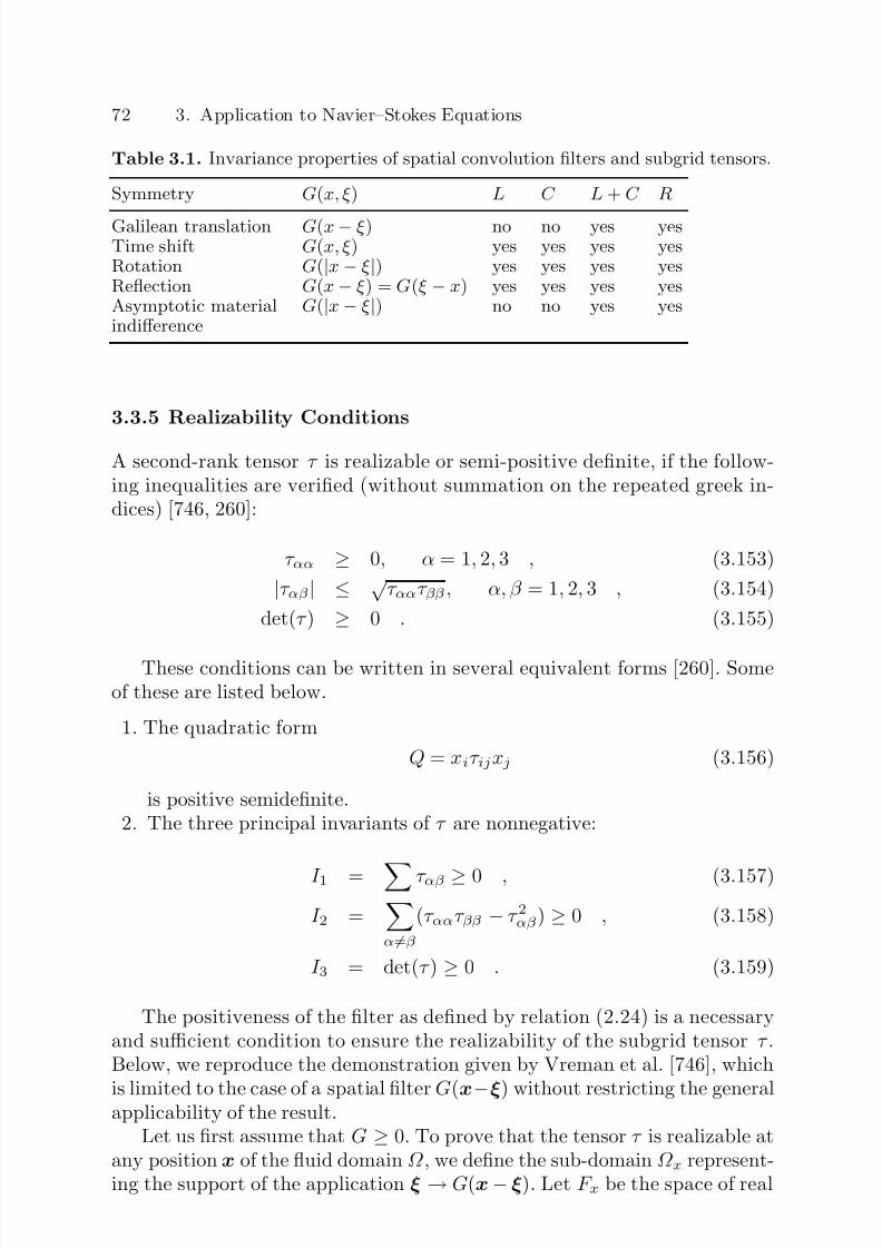
7/21/2019 Large Eddy Simulation for Incompressible Flows
http://slidepdf.com/reader/full/large-eddy-simulation-for-incompressible-flows 96/573
72 3. Application to Navier–Stokes Equations
Table 3.1. Invariance properties of spatial convolution filters and subgrid tensors.
Symmetry G(x, ξ) L C L + C R
Galilean translation G(x − ξ) no no yes yesTime shift G(x, ξ) yes yes yes yesRotation G(|x − ξ|) yes yes yes yesReflection G(x − ξ) = G(ξ − x) yes yes yes yesAsymptotic material G(|x − ξ|) no no yes yesindifference
3.3.5 Realizability Conditions
A second-rank tensor τ is realizable or semi-positive definite, if the follow-ing inequalities are verified (without summation on the repeated greek in-dices) [746, 260]:
τ αα ≥ 0, α = 1, 2, 3 , (3.153)
|τ αβ | ≤ √ τ αατ ββ , α, β = 1, 2, 3 , (3.154)
det(τ ) ≥ 0 . (3.155)
These conditions can be written in several equivalent forms [260]. Someof these are listed below.
1. The quadratic form
Q = xiτ ijxj (3.156)
is positive semidefinite.2. The three principal invariants of τ are nonnegative:
I 1 = τ αβ ≥ 0 , (3.157)
I 2 =α=β
(τ αατ ββ − τ 2αβ) ≥ 0 , (3.158)
I 3 = det(τ ) ≥ 0 . (3.159)
The positiveness of the filter as defined by relation (2.24) is a necessaryand sufficient condition to ensure the realizability of the subgrid tensor τ .Below, we reproduce the demonstration given by Vreman et al. [746], which
is limited to the case of a spatial filter G(x−ξ) without restricting the generalapplicability of the result.Let us first assume that G ≥ 0. To prove that the tensor τ is realizable at
any position x of the fluid domain Ω , we define the sub-domain Ω x represent-ing the support of the application ξ → G(x − ξ). Let F x be the space of real

7/21/2019 Large Eddy Simulation for Incompressible Flows
http://slidepdf.com/reader/full/large-eddy-simulation-for-incompressible-flows 97/573
3.3 Decomposition of the Non-linear Term. Conventional Approach 73
functions defined on Ω x. Since G is positive, for φ, ψ ∈ F x, the application
(φ, ψ)x = Ωx G(x − ξ)φ(ξ)ψ(ξ)dξ (3.160)
defines an inner product on F x. Using the definition of the filtering, thesubgrid tensor can be re-written in the form:
τ ij(x) = uiuj(x) − ui(x)uj(x)
= uiuj(x) − ui(x)uj(x) − uj(x)ui(x) + ui(x)uj(x)
= Ωx G(x
−ξ)ui(ξ)uj(ξ)d3ξ
−ui(x) Ωx G(x
−ξ)uj(ξ)d3ξ
− uj(x)
Ωx
G(x − ξ)ui(ξ)d3ξ − ui(x)uj(x)
Ωx
G(x − ξ)d3ξ
=
Ωx
G(x − ξ) (ui(ξ) − ui(x)) (uj(ξ) − uj(x))
= (uxi , uxj )x , (3.161)
where the difference uxi (ξ) = ui(ξ) − ui(x) is defined on Ω x. The tensor τ
thus appears as a Grammian 3 × 3 matrix of inner products, and is conse-quently always defined as semi-positive. This shows that the stated conditionis sufficient.
Let us now assume that the condition G ≥ 0 is not verified for a piecewisecontinuous kernel. There then exists a pair (x, y) ∈ Ω ×Ω , an ∈ IR+, > 0,and a neighbourhood V = ξ ∈ Ω, |ξ −y| < , such that G(x−ξ) < 0, ∀ξ ∈V . For a function u1 defined on Ω such that u1(ξ) = 0 if ξ ∈ V et u1(ξ) = 0everywhere else, then the component τ 11 is negative:
τ 11(x) = u21(x) − (u1(x))2
≤ V
G(x − ξ) (u1(ξ))2
d3ξ < 0 . (3.162)
The tensor τ is thus not semi-positive definite, which concludes thedemonstration. The properties of the three usual analytical filter presentedin Sect. 2.1.5 are summarized in Table 3.2.
Table 3.2. Positiveness property of convolution filters.
Filter Eq. Positiveness
Box (2.40) yesGaussian (2.42) yesSharp cutoff (2.44) no

7/21/2019 Large Eddy Simulation for Incompressible Flows
http://slidepdf.com/reader/full/large-eddy-simulation-for-incompressible-flows 98/573
74 3. Application to Navier–Stokes Equations
3.4 Extension to the Inhomogeneous Casefor the Conventional Approach
The results of the previous sections were obtained by applying isotropic homo-geneous filters on an unbounded domain to Navier–Stokes equations writtenin Cartesian coordinates. What is presented here are the equations obtainedby applying non-homogeneous convolution filters on bounded domains tothese equations. Using the commutator (2.13), the most general form of thefiltered Navier–Stokes equations is:
∂ui
∂t
+ ∂
∂xj
(uiuj) + ∂p
∂xi −ν
∂
∂xj ∂ui
∂xj
+ ∂uj
∂xi =
−
∂τ ij
∂xj
−
G, ∂
∂t
(ui) −
G,
∂
∂xj
(uiuj)
−
G, ∂
∂xi
( p) + ν
G,
∂ 2
∂xk∂xk
(ui) , (3.163)
∂ui∂xi
= −
G, ∂
∂xi
(ui) . (3.164)
All the terms appearing in the right-hand side of equations (3.163)and (3.164) are commutation errors. The first term of the right-hand sideof the filtered momentum equation is the subgrid force, and is subject tomodeling. The other terms are artefacts due to the filter, and escape subgridmodeling.
An interesting remark drawn from equation (3.164) is that the filteredfield is not divergence-free if some commutation errors arise. An analysis of the breakdown of continuity constraint in large-eddy simulation is providedby Langford and Moser [420], which shows that for many common large-
eddy simulation representations, there is no exact continuity constraint onthe filtered velocity field. But for mean-preserving representations a bulkcontinuity constraint holds.
The governing equations obtained using second-order commuting filters(SOCF), as well as the techniques proposed by Ghosal and Moin [262] andIovenio and Tordella [343] to reduce the commutation error and Vasilyev’shigh-order commuting filters [728], are presented in the following.
3.4.1 Second-Order Commuting Filter
Here we propose to generalize Leonard’s approach by applying SOCF filters.The decomposition of the non-linear term considered here as an example isthe triple decomposition; but the double decomposition is also usable. Forconvenience in writing the filtered equations, we introduce the operator Di

7/21/2019 Large Eddy Simulation for Incompressible Flows
http://slidepdf.com/reader/full/large-eddy-simulation-for-incompressible-flows 99/573
3.4 Extension to the Inhomogeneous Case for the Conventional Approach 75
such that:∂ψ
∂xi= Diψ . (3.165)
According to the results of Sect. 2.2.2, the operator Di is of the form:
Di = ∂
∂xi− α(2)∆
2Γ ijk
∂ 2
∂x2i
+ O(∆4
) , (3.166)
in which the term Γ is defined by the relation (2.147). By applying thefilter and bringing out the subgrid tensor τ ij = uiuj − uiuj , we get for themomentum equation:
∂ui∂t
+ Dj(uiuj) = −Di p + ν DjDjui − Djτ ij . (3.167)
To measure the errors, we introduce the expansion as a function of ∆:
p = p(0) + ∆2 p(1) + ... , (3.168)
u = u(0) + ∆2
u(1) + ... (3.169)
The terms corresponding to the odd powers of ∆ are identically zero
because of the symmetry of the convolution kernel. By substituting this de-composition in (3.167), at the first order we get:
∂u(0)i
∂t +
∂
∂xj
u
(0)i u
(0)j
= −∂p(0)
∂xi+ ν
∂
∂xj
∂u
(0)i
∂xj+
∂u(0)j
∂xi
− ∂τ
(0)ij
∂xj,
(3.170)
in which τ (0)ij is the subgrid term calculated from the field u(0). The associated
continuity equation is:
∂u(0)i
∂xi = 0 . (3.171)
These equations are identical to those obtained in the homogeneous case,
but relate to a variable containing an error in O(∆2
) with respect to theexact solution.
To reduce the error, the problem of the term in ∆2
has to be resolved, i.e.solve the equations that use the variables u(1) and p(1). Simple expansionslead to the system:
∂u(1)
i∂t + ∂
∂xj u(1)i u
(0)j + u
(0)i u
(1)j = −
∂p(1)
∂xi + ν ∂
∂xj ∂u(1)
i∂xj +∂u
(1)j
∂xi −∂τ
(1)ij
∂xj+ α(2)f
(1)i , (3.172)

7/21/2019 Large Eddy Simulation for Incompressible Flows
http://slidepdf.com/reader/full/large-eddy-simulation-for-incompressible-flows 100/573
76 3. Application to Navier–Stokes Equations
in which the coupling term f (1)i defined as:
f (1)i = Γ jmn
∂ 2(u(0)i u
(0)j )
∂xm∂xn+ Γ imn
∂ 2 p(0)
∂xm∂xn+ Γ jmn
∂ 2τ (0)ij
∂xm∂xn
− ν ∂Γ kmn
∂xk
∂ 2u(0)i
∂xm∂xn− 2Γ kmn
∂ 3u(0)i
∂xk∂xm∂xn, (3.173)
∂u(1)i
∂xi= 0 . (3.174)
By solving this second problem, we can ensure the accuracy of the solution
up to the order O(∆4
) .Another procedure aiming at removing the commutation error was pro-
posed by Iovenio and Tordella [343]. It relies on an approximation of thecommutation error terms up to the fourth order in terms of ∆ which is basedon the use of several filtering levels. Reminding that the commutation errorbetween the filtering operator and the first-order spatial derivative can beexpressed as
G,
d
dx
(φ) = −d∆(x)
dx
∂
∂∆φ∆
(x) , (3.175)
where φ∆
denotes the filtered quantity obtained applying a filter with length∆ on the variable φ, and introducing the central second order finite-differenceapproximation for the gradient of the filtered quantity with respect to thefilter width:
∂ ∂∆
φ∆
= 12hφ
∆+h − φ∆−h+ O(h2) (3.176)
one obtains the following explicit, two filtering level approximation for thecommutation error
G,
d
dx
(φ) −d∆(x)
dx
1
2∆
φ∆2∆
− φ∆
, (3.177)
This evaluation is independent of the exact filter shape, and makes it pos-sible to cancel the leading error term in each part of the filtered Navier-Stokesequations (3.163) - (3.164). It just involves the definition of an auxiliary fil-tering level with a cutoff length equal to 2∆.
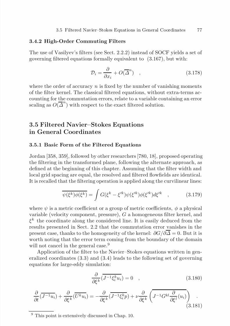
7/21/2019 Large Eddy Simulation for Incompressible Flows
http://slidepdf.com/reader/full/large-eddy-simulation-for-incompressible-flows 101/573
3.5 Filtered Navier–Stokes Equations in General Coordinates 77
3.4.2 High-Order Commuting Filters
The use of Vasilyev’s filters (see Sect. 2.2.2) instead of SOCF yields a set of
governing filtered equations formally equivalent to (3.167), but with:
Di = ∂
∂xi+ O(∆
n) , (3.178)
where the order of accuracy n is fixed by the number of vanishing momentsof the filter kernel. The classical filtered equations, without extra-terms ac-counting for the commutation errors, relate to a variable containing an errorscaling as O(∆
n) with respect to the exact filtered solution.
3.5 Filtered Navier–Stokes Equationsin General Coordinates
3.5.1 Basic Form of the Filtered Equations
Jordan [358, 359], followed by other researchers [780, 18], proposed operatingthe filtering in the transformed plane, following the alternate approach, asdefined at the beginning of this chapter. Assuming that the filter width andlocal grid spacing are equal, the resolved and filtered flowfields are identical.It is recalled that the filtering operation is applied along the curvilinear lines:
ψ(ξ k)φ(ξ k) =
G(ξ k − ξ k)ψ(ξ k)φ(ξ k)dξ k , (3.179)
where ψ is a metric coefficient or a group of metric coefficients, φ a physicalvariable (velocity component, pressure), G a homogeneous filter kernel, andξ k the coordinate along the considered line. It is easily deduced from the
results presented in Sect. 2.2 that the commutation error vanishes in thepresent case, thanks to the homogeneity of the kernel: ∂G/∂∆ = 0. But it isworth noting that the error term coming from the boundary of the domainwill not cancel in the general case.9
Application of the filter to the Navier–Stokes equations written in gen-eralized coordinates (3.3) and (3.4) leads to the following set of governingequations for large-eddy simulation:
∂
∂ξ k(J −1ξ ki ui) = 0 , (3.180)
∂
∂t(J −1ui) +
∂
∂ξ k(U kui) = − ∂
∂ξ k(J −1ξ ki p) + ν
∂
∂ξ k
J −1Gkl
∂
∂ξ l(ui)
.
(3.181)
9 This point is extensively discussed in Chap. 10.

7/21/2019 Large Eddy Simulation for Incompressible Flows
http://slidepdf.com/reader/full/large-eddy-simulation-for-incompressible-flows 102/573
78 3. Application to Navier–Stokes Equations
3.5.2 Simplified Form of the Equations – Non-linear TermsDecomposition
It is seen that many filtered nonlinear terms appear in (3.180) and (3.181)which originate from the coordinate transformation. In order to uncouplegeometrical quantities, such as metrics and Jacobian, from quantities relatedto the flow, like velocity, and to obtain a simpler problem, further assumptionsare required. The metrics being computed by a finite difference approximationin practice, they can be considered as filtered quantities, yielding:
U k = J −1ξ kj uj J −1 ξ kj uj . (3.182)
All the terms appearing in the filtered equations can be simplified simi-larly. As for the conventional approach, convective nonlinear terms need tobe decomposed in order to allow us to use them for practical purpose. Theresulting equations are:
∂
∂ξ k(U k) = 0 , (3.183)
∂
∂t(J −1ui) +
∂
∂ξ k(U k ui) = − ∂
∂ξ k(J −1ξ ki p) (3.184)
+ν ∂ ∂ξ k
J −1 Gkl ∂ ∂ξ l
(ui) − ∂ ∂ξ k
(σki ) ,
where the contravariant counterpart of the subgrid tensor is defined as
σki = J −1ξ kj uiuj − J −1ξ kj uj ui = U kui − U k ui . (3.185)
Taking into account the fact that the metrics are assumed to be smoothfiltered quantities, the contravariant subgrid tensor can be tied to the subgrid
tensor defined in Cartesian coordinates:σki = J −1ξ kj uiuj − J −1ξ kj uj ui = J −1 ξ kj (uiuj − uiuj) = J −1 ξ kj τ ij .
(3.186)
3.6 Closure Problem
3.6.1 Statement of the Problem
As was already said in the first chapter, large-eddy simulation is a techniquefor reducing the number of degrees of freedom of the solution. This is done byseparating the scales in the exact solution into two categories: resolved scalesand subgrid scales. The selection is made by the filtering technique describedabove.
7/21/2019 Large Eddy Simulation for Incompressible Flows
http://slidepdf.com/reader/full/large-eddy-simulation-for-incompressible-flows 103/573
3.6 Closure Problem 79
The complexity of the solution is reduced by retaining only the largescales in the numerical solution process, which entails reducing the numberof degrees of freedom in the solution in space and time. The informationconcerning the small scales is consequently lost, and none of the terms thatuse these scales, i.e. the terms in u in the physical space and in (1 − G)in the spectral space, can be calculated directly. They are grouped into thesubgrid tensor τ . This scale selection determines the level of resolution of themathematical model.
Nonetheless, in order for the dynamics of the resolved scales to remaincorrect, the subgrid terms have to be taken into consideration, and thus haveto be modeled. The modeling consists of approximating the coupling termson the basis of the information contained in the resolved scales alone. The
modeling problem is twofold:
1. Since the subgrid scales are lacking in the simulation, their existence isunknown and cannot be decided locally in space and time. The problemthus arises of knowing if the exact solution contains, at each point inspace and time, any smaller scales than the resolution established bythe filter. In order to answer this question, additional information hasto be introduced, in either of two ways. The first is to use additionalassumptions derived from acquired knowledge in fluid mechanics to linkthe existence of subgrid modes to certain properties of the resolved scales.The second way is to enrich the simulation by introducing new unknownsdirectly related to the subgrid modes, such as their kinetic energy, forexample.
2. Once the existence of the subgrid modes is determined, their interactionswith the resolved scales have to be reflected. The quality of the simulationwill depend on the fidelity with which the subgrid model reflects theseinteractions.
Various modeling strategies and models that have been developed are
presented in the following.An important remark, somewhat tautological, is that the modeling pro-cess should take into account the filtering operator [597, 171, 604]. This canbe seen by remarking that filtered and subgrid fields are defined by the filter-ing operator, and that a change in the filter will automatically lead to a newdefinition of these quantities and modify their properties.
3.6.2 Postulates
So far, we have assumed nothing concerning the type of flow at hand, aside
from those assumptions that allowed us to demonstrate the momentum andcontinuity equations. Subgrid modeling usually assumes the following hy-pothesis
Hypothesis 3.1 If subgrid scales exist, then the flow is locally (in space and time) turbulent.

7/21/2019 Large Eddy Simulation for Incompressible Flows
http://slidepdf.com/reader/full/large-eddy-simulation-for-incompressible-flows 104/573
80 3. Application to Navier–Stokes Equations
Consequently, the subgrid models will be built on the known propertiesof turbulent flows.
It should be noted that theories exist that use other basic hypotheses.We may mention as an example the description of suspensions in the form of a fluid with modified properties [423]: the solid particles are assumed to havepredefined characteristics (mass, form, spatial distribution, and so forth) andhave a characteristic size very much less than the filter cutoff length, i.e. at thescale at which we want to describe the flow dynamics directly. Their actionsare taken into account globally, which means a very high saving comparedwith an individual description of each particle. The different descriptionsobtained by homogenization techniques also enter into this framework.
3.6.3 Functional and Structural Modeling
Preliminary Remarks. Before discussing the various ways of modelingthe subgrid terms, we have to set some constraints in order to orient thechoices [627]. The subgrid modeling must be done in compliance with twoconstraints:
1. Physical constraint. The model must be consistent from the viewpoint of the phenomenon being modeled, i.e.:
– Conserve the basic properties of the starting equation, such as Galileaninvariance and asymptotic behaviors;
– Be zero wherever the exact solution exhibits no small scales corre-sponding to the subgrid scales;
– Induce an effect of the same kind (dispersive or dissipative, for exam-ple) as the modeled terms;
– Not destroy the dynamics of the solve scales, and thus especially notinhibit the flow driving mechanisms.
2. Numerical constraint. A subgrid model can only be thought of as included
in a numerical simulation method, and must consequently:– Be of acceptable algorithmic cost, and especially be local in time andspace;
– Not destabilize the numerical simulation;– Be insensitive to discretization, i.e. the physical effects induced theo-
retically by the model must not be inhibited by the discretization.
Modeling Strategies. The problem of subgrid modeling consists in takingthe interaction with the fluctuating field u, represented by the term ∇ · τ ,into account in the evolution equation of the filtered field u. Two modeling
strategies exist [627]:
– Structural modeling of the subgrid term, which consists in making the bestapproximation of the tensor τ by constructing it from an evaluation of uor a formal series expansion. The modeling assumption therefore consistsin using a relation of the form u = H(u) or τ = H(u).

7/21/2019 Large Eddy Simulation for Incompressible Flows
http://slidepdf.com/reader/full/large-eddy-simulation-for-incompressible-flows 105/573
3.6 Closure Problem 81
– Functional modeling , which consists in modeling the action of the subgridterms on the quantity u and not the tensor τ itself, i.e. introducing a dis-sipative or dispersive term, for example, that has a similar effect but notnecessarily the same structure (not the same proper axes, for example).The closure hypothesis can then be expressed in the form ∇ · τ = H(u).
These two modeling approaches do not require the same foreknowledgeof the dynamics of the equations treated and theoretically do not offer thesame potential in terms of the quality of results obtained.
The structural approach requires no knowledge of the nature of the inter-scale interaction, but does require enough knowledge of the structure of thesmall scales of the solution in order to be able to determine one of the relations
u = H(u) or τ = H(u) to be possible, one of the two following conditionshas to be met:
– The dynamics of the equation being computed leads to a universal form of the small scales (and therefore to their total structural independence fromthe resolved motion, as all that remains to be determined is their energylevel).
– The dynamics of the equation induces a sufficiently strong and simple inter-scale correlation for the structure of the subgrid scales to be deduced fromthe information contained in the resolved field.
As concerns the modeling of the inter-scale interaction by just takingits effect into account, this requires no foreknowledge of the subgrid scalestructure, but does require knowing the nature of the interaction [184] [383].Moreover, in order for such an approach to be practical, the effect of the smallscales on the large must be universal in character, and therefore independentof the large scales of the flow.
7/21/2019 Large Eddy Simulation for Incompressible Flows
http://slidepdf.com/reader/full/large-eddy-simulation-for-incompressible-flows 106/573
4. Other Mathematical Modelsfor the Large-Eddy Simulation Problem
The two preceding chapters are devoted to the convolution filtering math-ematical model for Large-Eddy simulation. Others approaches are now de-
scribed, that can be gouped in two classes:
– Mathematical models which rely on a statistical average (Sect. 4.1), recov-ering this way some interesting features of the Reynolds-Averaged Navier–Stokes model by precluding some drawbacks of the convolution filter ap-proach in general domains.
– Models derived from regularized versions of the Navier–Stokes equations(Sect. 4.2), that were proposed to alleviate some theoretical problems deal-ing with the existence, the uniqueness and the regularity of the general
solution of the three-dimensional, unsteady, incompressible Navier–Stokesequations. These regularized models have smooth solutions, in the sensethat their gradients remain controlled, and are re-interpreted within theLarge-Eddy Simulation framework as good candidates to account for theremoval of small scales.
4.1 Ensemble-Averaged Models
4.1.1 Yoshizawa’s Partial Statistical Average Model
Yoshizawa [791] proposes to combine scale decomposition and statistical av-erage to define an ad hoc mathematical model for Large-Eddy Simulation,referred to as the partial statistical average procedure . Writing the general-ized Fourier decomposition of a dummy variable φ(x, t) as
φ(x, t) =
k=1,+∞
φk(t)ψk(x) (4.1)
where φk(t) and ψk(x) are the coefficients of the decomposition and the basisfunctions, respectively, the filtered part of φ(x, t) is defined as
φ(x, t) =k=1,kc
φk(t)ψk(x) +
k=kc,+∞
φk(t)ψk(x) (4.2)
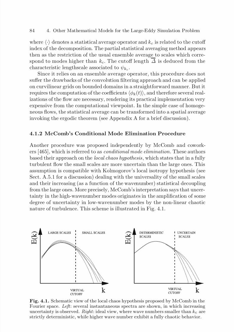
7/21/2019 Large Eddy Simulation for Incompressible Flows
http://slidepdf.com/reader/full/large-eddy-simulation-for-incompressible-flows 107/573
84 4. Other Mathematical Models for the Large-Eddy Simulation Problem
where · denotes a statistical average operator and kc is related to the cutoff index of the decomposition. The partial statistical averaging method appearsthen as the restriction of the usual ensemble average to scales which corre-spond to modes higher than kc. The cutoff length ∆ is deduced from thecharacteristic lengthscale associated to ψkc .
Since it relies on an ensemble average operator, this procedure does notsuffer the drawbacks of the convolution filtering approach and can be appliedon curvilinear grids on bounded domains in a straightforward manner. But itrequires the computation of the coefficients φk(t), and therefore several real-izations of the flow are necessary, rendering its practical implementation veryexpensive from the computational viewpoint. In the simple case of homoge-neous flows, the statistical average can be transformed into a spatial average
invoking the ergodic theorem (see Appendix A for a brief discussion).
4.1.2 McComb’s Conditional Mode Elimination Procedure
Another procedure was proposed independently by McComb and cowork-ers [465], which is referred to as conditional mode elimination . These authorsbased their approach on the local chaos hypothesis , which states that in a fullyturbulent flow the small scales are more uncertain than the large ones. Thisassumption is compatible with Kolmogorov’s local isotropy hypothesis (seeSect. A.5.1 for a discussion) dealing with the universality of the small scalesand their increasing (as a function of the wavenumber) statistical decouplingfrom the large ones. More precisely, McComb’s interpretation says that uncer-tainty in the high-wavenumber modes originates in the amplification of somedegree of uncertainty in low-wavenumber modes by the non-linear chaoticnature of turbulence. This scheme is illustrated in Fig. 4.1.
Fig. 4.1. Schematic view of the local chaos hypothesis proposed by McComb in theFourier space. Left : several instantaneous spectra are shown, in which increasinguncertainty is observed. Right : ideal view, where wave numbers smaller than kc arestrictly deterministic, while higher wave number exhibit a fully chaotic behavior.
7/21/2019 Large Eddy Simulation for Incompressible Flows
http://slidepdf.com/reader/full/large-eddy-simulation-for-incompressible-flows 108/573
4.2 Regularized Navier–Stokes Models 85
The scale separation with a cutoff length ∆ is achieved carying out a con-ditional statistical average of scales smaller than ∆, φ<, based on fixed real-izations of scales larger than ∆, φ>. The former are assumed to be uncertainand to exhibit and infinite number of different realizations for each realizationof the large scales.
The filtered part of φ(x, t) is then expressed as
φ(x, t) = φ>(x, t) + φ<|φ>(x, t) (4.3)
where f |g denotes the conditional statistical average of f with respect tog.
As Yoshizawa’s procedure, the conditional mode elimination does not suf-fer the drawbacks of the filtering approach. These two ensemble-average basedmodels for Large-Eddy Simulation are equivalent in many cases.
4.2 Regularized Navier–Stokes Models
The mathematical models discussed in this section were not originally pro-posed to represent the properties of the Large-Eddy Simulation technique.They are surrogates to the Navier–Stokes equations, which have better prop-erties from the pure mathematical point of view: while the question of the
existence, uniqueness and regulatity of the solution of the three-dimensional,unsteady and incompressible Navier–Stokes equations is still an open prob-lem, these new models allow for a complete mathematical analysis. One of the main obstacle faced in the mathematical analysis of the Navier–Stokesequations is that it cannot yet be proven that its solutions remain smooth forarbitrarily long times. More precisely, no a priori estimates has been foundwhich guarantees that the enstrophy remains finite everywhere in the domainfilled by the fluid (but it can be proven that it is bounded in the mean). Thephysical interpretation associated with this picture is that some very inter-
mittent vorticity bursts can occur, injecting kinetic energy at scales muchsmaller than the Kolmorogov scale, resulting in quasi-infinite local valuesof the enstrophy. Such events correspond to finite-time singularities of thesolution, and violate the axiom of continuum mechanics.
A large number of mathematical results dealing with these problems havebeen published, which will not be further discussed here. The important pointis that some systems, which are very close to the Navier–Stokes equations,have been proposed. A common feature is that they are well-posed from themathematical point of view, meaning that their solutions are proved to be
regular. As a consequence, they appear as regularized systems derived fromthe original Navier–Stokes equations, the regularization being associated tothe disappearance of singularities. From a physical point of view, these newsystems do not allow the occurance of local infinite gradient thanks to anextra damping of the smallest scales. This smoothing property originatestheir interpretation as models for Large-Eddy Simulation.

7/21/2019 Large Eddy Simulation for Incompressible Flows
http://slidepdf.com/reader/full/large-eddy-simulation-for-incompressible-flows 109/573
86 4. Other Mathematical Models for the Large-Eddy Simulation Problem
4.2.1 Leray’s Model
The first model was proposed by Leray in 1934, who suggested to regularize
the Navier–Stokes equations as follows:
∂ui∂t
+ ∂ukui
∂xk= − ∂p
∂xi+ ν
∂ 2ui∂xk∂xk
(4.4)
∂ui∂xi
= 0 (4.5)
where the regularized (i.e. filtered) velocity field is defined as
u(x, t) = φ u(x, t) (4.6)
where the mollifying function (i.e. the filter kernel) φ is assumed to havea compact support, to be C ∞ and to have an integral equal to one. It canbe proved under these assumptions that the solution of the regularized sys-tem (4.4)–(4.5) is unique and C ∞. A main drawback is that it does not shareall the frame-invariance properties of the Navier–Stokes equations. As quotedby Geurts and Holm [258], the system proposed by Leray can be rewrittenin the usual Large-Eddy Simulation framework applying the filter a second
times, leading to
∂ui∂t
+ ∂uk ui
∂xk= − ∂p
∂xi+ ν
∂ 2ui∂xk∂xk
− ∂τ Lerayij
∂xj(4.7)
∂ui∂xi
= 0 (4.8)
where the subgrid tensor ansatz is defined as
τ Lerayij = ui uj − uiuj (4.9)
An important difference with the usual definition of the subgrid tensorτ ij is that this new tensor is not symmetric. Leray’s regularized model makesit possible to carry out a complete mathematical analysis, but suffers thesame problem when dealing with curvilinear grids on bounded domains asthe original convolution filter model described in the preceding chapters.
4.2.2 Holm’s Navier–Stokes-α Model
The second regularized model presented in this chapter is the Navier–Stokes-α proposed by Holm (see [221, 282, 182, 221, 258, 281]). The regularizationis achieved by imposing an energy penalty which damps the scales smallerthan the threshold scale α (to be interpreted as ∆ within the usual large-

7/21/2019 Large Eddy Simulation for Incompressible Flows
http://slidepdf.com/reader/full/large-eddy-simulation-for-incompressible-flows 110/573
4.2 Regularized Navier–Stokes Models 87
eddy simulation framework)1, while still allowing for non linear sweeping of the small scales by the largest ones. The regularization appears as a non-linearly dispersive modification of the convection term in the Navier–Stokesequations.
The system of the Navier–Stokes-α (also referred to as the Camassa-Holmequations) can be derived in two different ways, which are now presented.
Method 1: Kelvin-filtered Navier–Stokes equations. The first way toobtain the Navier–Stokes-α model is to introduce the Kelvin-filtering. TheNavier–Stokes equations satisfy Kelvin’s circulation theorem
d
dt Γ (u)
u
·dx = Γ (u)
(ν
∇2)
·dx (4.10)
where Γ (u) is a closed fluid loop that moves with velocity u. The originalset of equations is regularized by modifying the fluid loop along which thecirculation is integrated: instead of using a fluid loop moving at velocity u,an new fluid loop moving at the regularized velocity u is considered. Theexact definition of u is not necessary at this point and will be given later.The new circulation relationship is
ddt Γ (u)u · dx =
Γ (u)(ν ∇2) · dx (4.11)
and corresponds to the following modified momentum equation:
∂ u
∂t + u · ∇u + ∇T u · u = −∇ p + ν ∇2u (4.12)
with
∇ · u = 0 . (4.13)This set of equations describes the Kelvin-filtered Navier–Stokes equa-
tions. The Navier–Stokes-α equations are recovered specifying the regularizedfield u as the result of the application of the Helmholtz filter (2.35) to theoriginal field u:
u = (1 − α2∇2)u . (4.14)
It can be proved that the kinetic energy E α defined as
E α = 12
u · udx = 12|u|2 +
α2
2 |∇2u|2 dx , (4.15)
1 It can be shown that in the case of three-dimensional fully developed turbulence,the solution of the Navier–Stokes-α exhibits the usual k−5/3 behavior for scaleslarger than α and a k−3 behavior for scales smaller than α.
7/21/2019 Large Eddy Simulation for Incompressible Flows
http://slidepdf.com/reader/full/large-eddy-simulation-for-incompressible-flows 111/573
88 4. Other Mathematical Models for the Large-Eddy Simulation Problem
is bounded, showing that the filtered field u remains regular. The equa-tion (4.12) can be rewritten under the usual form in Large-Eddy Simulationas a momentum equation for the filtered velocity field u (formally identicalto (4.4)). The corresponding definition of the subgrid tensor is
τ NSαij = (ui uj − ui uj) − α2
∂uk∂xi
∂uk∂xj
+ uj∇2ui
. (4.16)
Method 2: Modified Leray’s Model. Guermond, Oden and Prud-homme [282] observe that the Navier–Stokes-α system can be interpreted asa frame-invariant modification of original Leray’s regularized model. Startingfrom the rotational form of the Navier–Stokes equations
∂ u
∂t + (∇ × u) × u = −∇π + ν ∇2u, π = p +
1
2u2 , (4.17)
∇ · u = 0 , (4.18)
and regularizing it using the technique proposed by Leray, one obtains
∂ u
∂t + (∇ × u) × u = −∇π + ν ∇2
u, π = p +
1
2 u
2
, (4.19)
∇ · u = 0 . (4.20)
Now using the relations
(∇ × u) × u = u · ∇u − (∇T u)u, ∇(u · (∇T u)) = (∇T u)u + (∇T u)u ,(4.21)
the following form of the regularized system is recovered
∂ u
∂t + u · ∇u + (∇T u) · u = −∇π + ν ∇2u, π = π − u · u , (4.22)
∇ · u = 0 . (4.23)
The Navier–Stokes-α model is obatined using the Helmholtz filter (4.14).The corresponding equation for u is
∂ u
∂t + u · ∇u = ∇ · T , (4.24)
with
T = − pId + 2ν (1 − α2∇2)S + 2α2S
, (4.25)
7/21/2019 Large Eddy Simulation for Incompressible Flows
http://slidepdf.com/reader/full/large-eddy-simulation-for-incompressible-flows 112/573
4.2 Regularized Navier–Stokes Models 89
where S
is related to the Jaumann derivative of the regularized strain ratetensor:
S
= ∂S
∂t + u · ∇S + SΩ − ΩS, Ω =
1
2
∇u − ∇T u . (4.26)
This system is formally similar to the constitutive law of a rate-dependentincompressible fluid of second grade with slightly modified dissipation, and itis frame-invariant. It is equivalent to the Leray model in which the term whichis responsible for the failure in the frame preservation, i.e. α2(∇T u∇2u), hasbeen removed. Therefore, the Navier–Stokes-α equations appear as a pertur-
bation of order α2 (i.e. ∆2
) of the original Leray model.
4.2.3 Ladyzenskaja’s Model
Another regularized version of the Navier–Stokes equations was proposedby Ladyzenskaja and Kaniel [417, 418, 377], who introduced a non-linearmodification of the stress tensor which is expected to be more relevant thanthe linear relationship for Newtonian fluids when velocity gradients are large.The equation for the regularized field u is
∂ u∂t
+ u · ∇u = −∇ p + ν ∇2u − ε∇ · T (∇u) , (4.27)
∇ · u = 0 , (4.28)
where ε is a strictly arbitrary constant and the non-linear stress tensor T isdefined as
T (∇u) = ν T (∇u2)∇u , (4.29)
where the non-linear viscosity ν T (τ ) is a positive monotonically-increasingfunction of τ ≥ 0 that obeys the following law for large values of τ :
cτ µ ≤ ν T (τ ) ≤ cτ µ, 0 < c < c, µ ≥ 1
4 . (4.30)
The equivalent expression for the subgrid stress tensor is
τ Ladyzenskajaij = εT ij(∇u2) . (4.31)
Since T depends only on the gradient of the resolved field u, Ladyzen-skaja’s model is closed and does not require further modeling work.
7/21/2019 Large Eddy Simulation for Incompressible Flows
http://slidepdf.com/reader/full/large-eddy-simulation-for-incompressible-flows 113/573
5. Functional Modeling (Isotropic Case)
It would be illusory to try to describe the structure of the scales of motionand the interactions in all imaginable configurations, in light of the very large
disparity of physical phenomena encountered. So we have to restrict this de-scription to cases which by nature include scales that are too small for today’scomputer facilities to solve them entirely, and which are at the same time ac-cessible to theoretical analysis. This description will therefore be centered onthe inter-scale interactions in the case of fully developed isotropic homoge-neous turbulence1, which is moreover the only case accessible by theoreticalanalysis and is consequently the only theoretical framework used today fordeveloping subgrid models. Attempts to extend this theory to anisotropicand/or inhomogeneous cases are discussed in Chap. 6. The text will mainly
be oriented toward the large-eddy simulation aspects. For a detailed descrip-tion of the isotropic homogeneous turbulence properties, which are reviewedin Appendix A, the reader may refer to the works of Lesieur [439] and Batch-elor [45].
5.1 Phenomenology of Inter-Scale Interactions
It is important to note here the framework of restrictions that apply to the
results we will be presenting. These results concern three-dimensional flowsand thus do not cover the physics of two-dimensional flows (in the senseof flows with two directions2, and not two-component3 flows), which havea totally different dynamics [403, 404, 405, 438, 481]. The modeling in thetwo-dimensional case leads to specific models [42, 624, 625] which will not
1 That is, whose statistical properties are invariant by translation, rotation, orsymmetry.
2 These are flows such that there exists a direction x for which we have the prop-erty:
∂ u∂x
≡ 0 .
3 These are flows such that there exists a framework in which the velocity fieldhas an identically zero component.

7/21/2019 Large Eddy Simulation for Incompressible Flows
http://slidepdf.com/reader/full/large-eddy-simulation-for-incompressible-flows 114/573
92 5. Functional Modeling (Isotropic Case)
be presented. For details on two-dimensional turbulence, the reader may alsorefer to [439].
5.1.1 Local Isotropy Assumption: Consequences
In the case of fully developed turbulence, Kolmogorov’s statistical descriptionof the small scales of the flow, based on the assumption of local isotropy, hasbeen the one most used for a very long time.
By introducing the idea of local isotropy, Kolmogorov assumes that thesmall scales belonging to the inertial range of the energy spectrum of a fullydeveloped inhomogeneous turbulent flow are:
– Statistically isotropic , and therefore entirely characterized by a character-istic velocity and time;– Without time memory , therefore in energy equilibrium with the large scales
of the flow by instantaneous re-adjustment.
This isotropy of the small scales implies that they are statistically inde-pendent of the large energetic scales, which are characteristic of each flowand are therefore anisotropic. Experimental work [512] has shown that thisassumption is not valid in shear flows for all the scales belonging to the in-ertial range, but only for those whose size is of the order of the Kolmogorov
scale. Numerical experiments [32] show that turbulent stresses are nearlyisotropic for wave numbers k such that kLε > 50, where Lε is the integraldissipation length4. These experiments have also shown that the existenceof an inertial region does not depend on the local isotropy hypothesis. Thecauses of this persistence of the anisotropy in the inertial range due to in-teractions existing between the various scales of the flow will be mentionedin Chap. 6. Works based on direct numerical simulations have also shownthat the assumption of equilibrium between the resolved and subgrid scalesmay be faulted, at least temporarily, when the flow is subject to unsteady
forcing [594, 570, 454, 504]. This is due to the fact that the relaxation timesof these two scale ranges are different. In the case of impulsively acceleratedflows (plane channel, boundary layer, axisymmetric straining) the subgridscales react more quickly than the resolved ones, and then also relax morequickly toward an equilibrium solution.
The existence of a zone of the spectrum, corresponding to the higher fre-quencies, where the scales of motion are statistically isotropic, justifies thestudy of the inter-modal interactions in the ideal case of isotropic homoge-neous turbulence. Strictly speaking, the results can be used for determining
subgrid models only if the cutoff associated with the filter is in this region,4 The integral dissipation length is defined as
Lε = uiui3/2
ε ,
where ε is the energy dissipation rate.

7/21/2019 Large Eddy Simulation for Incompressible Flows
http://slidepdf.com/reader/full/large-eddy-simulation-for-incompressible-flows 115/573
5.1 Phenomenology of Inter-Scale Interactions 93
because the dynamics of the unresolved scales then corresponds well to thatof the isotropic homogeneous turbulence. It should be noted that this lastcondition implies that the representation of the dynamics, while incomplete,is nonetheless very fine, which theoretically limits the gain in complexity thatcan be expected from large-eddy simulation technique.
Another point is that the local isotropy hypothesis is formulated for fullydeveloped turbulent flows at very high Reynolds numbers. As it affirms theuniversal character of the small scales’ behavior for these flows, it ensuresthe possibility using the large-eddy simulation technique strictly, if the filtercutoff frequency is set sufficiently high. There is no theoretical justification,though, for applying the results of this analysis to other flows, such as tran-sitional flows.
5.1.2 Interactions Between Resolved and Subgrid Scales
In order to study the interactions between the resolved and subgrid scales,we adopt an isotropic filter by a cutoff wave number kc. The subgrid scalesare those represented by the k modes such that k ≥ kc.
In the case of fully developed isotropic homogeneous turbulence, the sta-tistical description of the inter-scale interactions is reduced to that of thekinetic energy transfers. Consequently, only the information associated withthe amplitude of the fluctuations is conserved, and none concerning the phaseis taken into account.
These transfers are analyzed using several tools:
– Analytical theories of turbulence, also called two-point closures, which de-scribe triadic interactions on the basis of certain assumptions. They willtherefore express the non-linear term S (k| p, q), defined by relation (3.50)completely. For a description of these theories, the reader may refer toLesieur’s book [439], and we also mention Waleffe’s analysis [748, 749],
certain conclusions of which are presented in the following.– Direct numerical simulations, which provide a complete description of the
dynamics.– Renormalization Group Theory [622, 328, 812, 809, 464, 775, 804, 805, 813,
802, 803, 810], with several variants.
Typology of the Triadic Interactions. It appears from the developmentsof Sect. 3.1.3 (also see Appendix A) that the
u(k) mode interacts only with
those modes whose wave vectors p and q form a closed triangle with k. Thewave vector triads (k, p, q) thus defined are classified in several groups [805]which are represented in Fig. 5.1:
– Local triads for which
1
a ≤ max
p
k, q
k
≤ a, a = O(1) ,
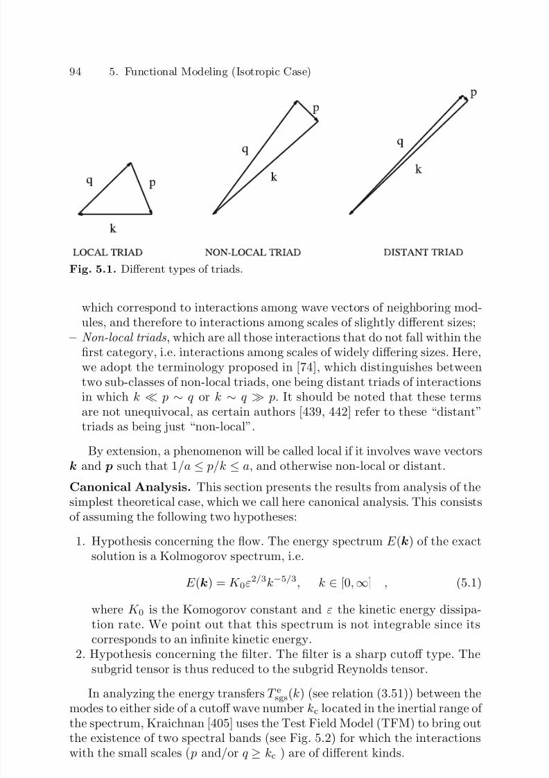
7/21/2019 Large Eddy Simulation for Incompressible Flows
http://slidepdf.com/reader/full/large-eddy-simulation-for-incompressible-flows 116/573
94 5. Functional Modeling (Isotropic Case)
Fig. 5.1. Different types of triads.
which correspond to interactions among wave vectors of neighboring mod-ules, and therefore to interactions among scales of slightly different sizes;
– Non-local triads , which are all those interactions that do not fall within thefirst category, i.e. interactions among scales of widely differing sizes. Here,we adopt the terminology proposed in [74], which distinguishes betweentwo sub-classes of non-local triads, one being distant triads of interactionsin which k p ∼ q or k ∼ q p. It should be noted that these terms
are not unequivocal, as certain authors [439, 442] refer to these “distant”triads as being just “non-local”.
By extension, a phenomenon will be called local if it involves wave vectorsk and p such that 1/a ≤ p/k ≤ a, and otherwise non-local or distant.
Canonical Analysis. This section presents the results from analysis of thesimplest theoretical case, which we call here canonical analysis. This consistsof assuming the following two hypotheses:
1. Hypothesis concerning the flow. The energy spectrum E (k) of the exactsolution is a Kolmogorov spectrum, i.e.
E (k) = K 0ε2/3k−5/3, k ∈ [0,∞] , (5.1)
where K 0 is the Komogorov constant and ε the kinetic energy dissipa-tion rate. We point out that this spectrum is not integrable since itscorresponds to an infinite kinetic energy.
2. Hypothesis concerning the filter. The filter is a sharp cutoff type. Thesubgrid tensor is thus reduced to the subgrid Reynolds tensor.
In analyzing the energy transfers T esgs(k) (see relation (3.51)) between themodes to either side of a cutoff wave number kc located in the inertial range of the spectrum, Kraichnan [405] uses the Test Field Model (TFM) to bring outthe existence of two spectral bands (see Fig. 5.2) for which the interactionswith the small scales ( p and/or q ≥ kc ) are of different kinds.

7/21/2019 Large Eddy Simulation for Incompressible Flows
http://slidepdf.com/reader/full/large-eddy-simulation-for-incompressible-flows 117/573
5.1 Phenomenology of Inter-Scale Interactions 95
Fig. 5.2. Interaction regions between resolved and subgrid scales.
1. In the first region (1 in Fig. 5.2), which corresponds to the modes such
that k kc, the dominant dynamic mechanism is a random displace-ment of the momentum associated with k by disturbances associatedwith p and q. This phenomenon, analogous to the effects of the molecu-lar viscosity, entails a kinetic energy decay associated with k and, sincethe total kinetic energy is conserved, a resulting increase of it associatedwith p and q. So here it is a matter of a non-local transfer of energy asso-ciated with non-local triadic interactions. These transfers, which inducea damping of the fluctuations, are associated with what Waleffe [748, 749]classifies as type F triads (represented in Fig. 5.3).
Fig. 5.3. Non-local triad (k, p,q) of the F type according to Waleffe’s classifica-tion, and the associated non-local energy transfers. The kinetic energy of the modecorresponding to the smallest wave vector k is distributed to the other two modes p and q, creating a forward energy cascade in the region where k kc.
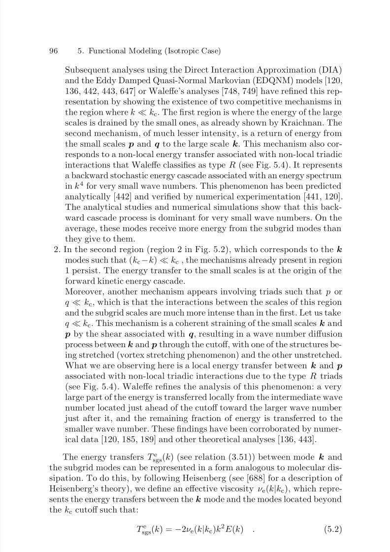
7/21/2019 Large Eddy Simulation for Incompressible Flows
http://slidepdf.com/reader/full/large-eddy-simulation-for-incompressible-flows 118/573
96 5. Functional Modeling (Isotropic Case)
Subsequent analyses using the Direct Interaction Approximation (DIA)and the Eddy Damped Quasi-Normal Markovian (EDQNM) models [120,136, 442, 443, 647] or Waleffe’s analyses [748, 749] have refined this rep-resentation by showing the existence of two competitive mechanisms inthe region where k kc. The first region is where the energy of the largescales is drained by the small ones, as already shown by Kraichnan. Thesecond mechanism, of much lesser intensity, is a return of energy fromthe small scales p and q to the large scale k. This mechanism also cor-responds to a non-local energy transfer associated with non-local triadicinteractions that Waleffe classifies as type R (see Fig. 5.4). It representsa backward stochastic energy cascade associated with an energy spectrumin k4 for very small wave numbers. This phenomenon has been predicted
analytically [442] and verified by numerical experimentation [441, 120].The analytical studies and numerical simulations show that this back-ward cascade process is dominant for very small wave numbers. On theaverage, these modes receive more energy from the subgrid modes thanthey give to them.
2. In the second region (region 2 in Fig. 5.2), which corresponds to the k
modes such that (kc−k) kc , the mechanisms already present in region1 persist. The energy transfer to the small scales is at the origin of theforward kinetic energy cascade.
Moreover, another mechanism appears involving triads such that p orq kc, which is that the interactions between the scales of this regionand the subgrid scales are much more intense than in the first. Let us takeq kc. This mechanism is a coherent straining of the small scales k and
p by the shear associated with q, resulting in a wave number diffusionprocess between k and p through the cutoff, with one of the structures be-ing stretched (vortex stretching phenomenon) and the other unstretched.What we are observing here is a local energy transfer between k and p
associated with non-local triadic interactions due to the type R triads
(see Fig. 5.4). Waleffe refines the analysis of this phenomenon: a verylarge part of the energy is transferred locally from the intermediate wavenumber located just ahead of the cutoff toward the larger wave number
just after it, and the remaining fraction of energy is transferred to thesmaller wave number. These findings have been corroborated by numer-ical data [120, 185, 189] and other theoretical analyses [136, 443].
The energy transfers T esgs(k) (see relation (3.51)) between mode k andthe subgrid modes can be represented in a form analogous to molecular dis-sipation. To do this, by following Heisenberg (see [688] for a description of Heisenberg’s theory), we define an effective viscosity ν e(k|kc), which repre-sents the energy transfers between the k mode and the modes located beyondthe kc cutoff such that:
T esgs(k) = −2ν e(k|kc)k2E (k) . (5.2)

7/21/2019 Large Eddy Simulation for Incompressible Flows
http://slidepdf.com/reader/full/large-eddy-simulation-for-incompressible-flows 119/573
5.1 Phenomenology of Inter-Scale Interactions 97
Fig. 5.4. Non-local (k, p,q) triad of the R type according to Waleffe’s classification,and the associated energy transfers in the case q kc. The kinetic energy of themode corresponding to the intermediate wave vector k is distributed locally to the
largest wave vector p and non-locally to the smallest wave vector, q. The formertransfer originates the intensification of the coupling in the (kc − k) kc spectralband, while the latter originates the backward kinetic energy cascade.
It should be pointed out that this viscosity is real, i.e. ν e(k|kc) ∈ IR, andthat if any information related to the phase were included, it would leadthe definition of a complex term having an a priori non-zero imaginary part,which may seem to be more natural for representing a dispersive type of coupling. Such a term is obtained not by starting with the kinetic energy
equation, but with the momentum equation5
.The two energy cascades, forward and backward, can be introduced sepa-
rately by introducing distinct effective viscosities, constructed in such a wayas to ensure energy transfers equivalent to those of these cascades. We getthe following two forms:
ν +e (k|kc, t) = −T +sgs(k|kc, t)
2k2E (k, t) , (5.3)
ν −e (k|kc, t) = −T −sgs(k|kc, t)2k2E (k, t)
, (5.4)
in which T +sgs(k|kc, t) (resp. T −sgs(k|kc, t)) is the energy transfer term from thek mode to the subgrid modes (resp. from the subgrid modes to the k mode).This leads to the decomposition:
T esgs(k) = T +sgs(k|kc, t) + T −sgs(k|kc, t) (5.5)
= −2k2E (k, t) ν +e (k|kc, t) + ν −e (k|kc, t) . (5.6)
These two viscosities depend explicitly on the wave number k and thecutoff wave vector kc, as well as the shape of the spectrum. The result of
5 This possibility is only mentioned here, because no works have been publishedon it to date.
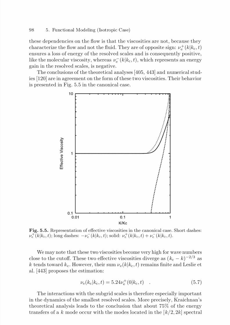
7/21/2019 Large Eddy Simulation for Incompressible Flows
http://slidepdf.com/reader/full/large-eddy-simulation-for-incompressible-flows 120/573
98 5. Functional Modeling (Isotropic Case)
these dependencies on the flow is that the viscosities are not, because theycharacterize the flow and not the fluid. They are of opposite sign: ν +e (k|kc, t)ensures a loss of energy of the resolved scales and is consequently positive,like the molecular viscosity, whereas ν −e (k|kc, t), which represents an energygain in the resolved scales, is negative.
The conclusions of the theoretical analyses [405, 443] and numerical stud-ies [120] are in agreement on the form of these two viscosities. Their behavioris presented in Fig. 5.5 in the canonical case.
Fig. 5.5. Representation of effective viscosities in the canonical case. Short dashes:ν +e (k|kc, t); long dashes: −ν −e (k|kc, t); solid: ν +e (k|kc, t) + ν −e (k|kc, t).
We may note that these two viscosities become very high for wave numbersclose to the cutoff. These two effective viscosities diverge as (kc − k)−2/3 ask tends toward kc. However, their sum ν e(k|kc, t) remains finite and Leslie etal. [443] proposes the estimation:
ν e
(kc|
kc
, t) = 5.24ν +e
(0|k
c, t) . (5.7)
The interactions with the subgrid scales is therefore especially importantin the dynamics of the smallest resolved scales. More precisely, Kraichnan’stheoretical analysis leads to the conclusion that about 75% of the energytransfers of a k mode occur with the modes located in the [k/2, 2k] spectral

7/21/2019 Large Eddy Simulation for Incompressible Flows
http://slidepdf.com/reader/full/large-eddy-simulation-for-incompressible-flows 121/573
5.1 Phenomenology of Inter-Scale Interactions 99
band6. No transfers outside this spectral band have been observed in directnumerical simulations at low Reynolds numbers [185, 804, 805]. The differ-ence with the theoretical analysis stems from the fact that this analysis isperformed in the limit of the infinite Reynolds numbers.
In the limit of the very small wave numbers, we have the asymptoticbehaviors:
2k2E (k, t)ν +e (k|kc, t) ∝ k1/3 , (5.8)
2k2E (k, t)ν −e (k|kc, t) ∝ k4 . (5.9)
The effective viscosity associated with the energy cascade takes the con-stant asymptotic value:
ν +e (0|kc, t) = 0.292ε1/3k−4/3c . (5.10)
We put the emphasis on the fact that the effective viscosity discussedhere is defined considering the kinetic enery transfer between unresolved andresolved modes. As quoted by McComb et al. [465], it is possible to definedifferent effective viscosities by considering other balance equations, suchas the enstrophy transfer. An important consequence is that kinetic-energy-based effective viscosities are efficient surrogates of true transfer terms inthe kinetic energy equation, but may be very bad representations of subgrid
effects for other physical mechanisms.
Dependency According to the Filter. Leslie and Quarini [443] extendedthe above analysis to the case of the Gaussian filter. The spectrum consideredis always of the Kolmogorov type. The Leonard term is now non-zero. Theresults of the analysis show very pronounced differences from the canonicalanalysis. Two regions of the spectrum are still distinguishable, though, withregard to the variation of the effective viscosities ν +e and ν −e , which are shownin Fig. 5.6:
– In the first region, where k kc, the transfer terms still observe a constantasymptotic behavior, independent of the wave number considered, as in thecanonical case. The backward cascade term is negligible compared with theforward cascade term.
– In the second region, on the other hand, when approaching cutoff, the twotransfer terms do not have divergent behavior, contrary to what is observedin the canonical case. The forward cascade term decreases monotonicallyand cancels out after the cutoff for wave numbers more than a decadebeyond it. The backward cascade term increases up to cutoff and exhibits
a decreasing behavior analogous to that of the forward cascade term. Themaximum intensity of the backward cascade is encountered for modes justafter the cutoff.
6 The same local character of kinetic energy transfer is observed in non-homogeneous flow, such has the plane channel flow [186].
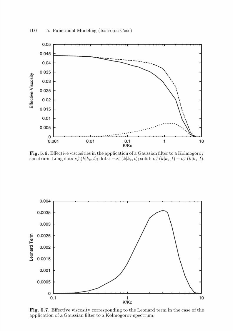
7/21/2019 Large Eddy Simulation for Incompressible Flows
http://slidepdf.com/reader/full/large-eddy-simulation-for-incompressible-flows 122/573
100 5. Functional Modeling (Isotropic Case)
Fig. 5.6. Effective viscosities in the application of a Gaussian filter to a Kolmogorovspectrum. Long dots ν +e (k|kc, t); dots: −ν −e (k|kc, t); solid: ν +e (k|kc, t) + ν −e (k|kc, t).
Fig. 5.7. Effective viscosity corresponding to the Leonard term in the case of theapplication of a Gaussian filter to a Kolmogorov spectrum.
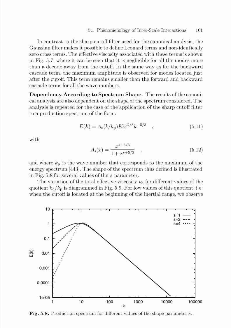
7/21/2019 Large Eddy Simulation for Incompressible Flows
http://slidepdf.com/reader/full/large-eddy-simulation-for-incompressible-flows 123/573
5.1 Phenomenology of Inter-Scale Interactions 101
In contrast to the sharp cutoff filter used for the canonical analysis, theGaussian filter makes it possible to define Leonard terms and non-identicallyzero cross terms. The effective viscosity associated with these terms is shownin Fig. 5.7, where it can be seen that it is negligible for all the modes morethan a decade away from the cutoff. In the same way as for the backwardcascade term, the maximum amplitude is observed for modes located justafter the cutoff. This term remains smaller than the forward and backwardcascade terms for all the wave numbers.
Dependency According to Spectrum Shape. The results of the canoni-cal analysis are also dependent on the shape of the spectrum considered. Theanalysis is repeated for the case of the application of the sharp cutoff filter
to a production spectrum of the form:
E (k) = As(k/kp)K 0ε2/3k−5/3 , (5.11)
with
As(x) = xs+5/3
1 + xs+5/3 , (5.12)
and where kp is the wave number that corresponds to the maximum of theenergy spectrum [443]. The shape of the spectrum thus defined is illustratedin Fig. 5.8 for several values of the s parameter.
The variation of the total effective viscosity ν e for different values of thequotient kc/kp is diagrammed in Fig. 5.9. For low values of this quotient, i.e.when the cutoff is located at the beginning of the inertial range, we observe
Fig. 5.8. Production spectrum for different values of the shape parameter s.
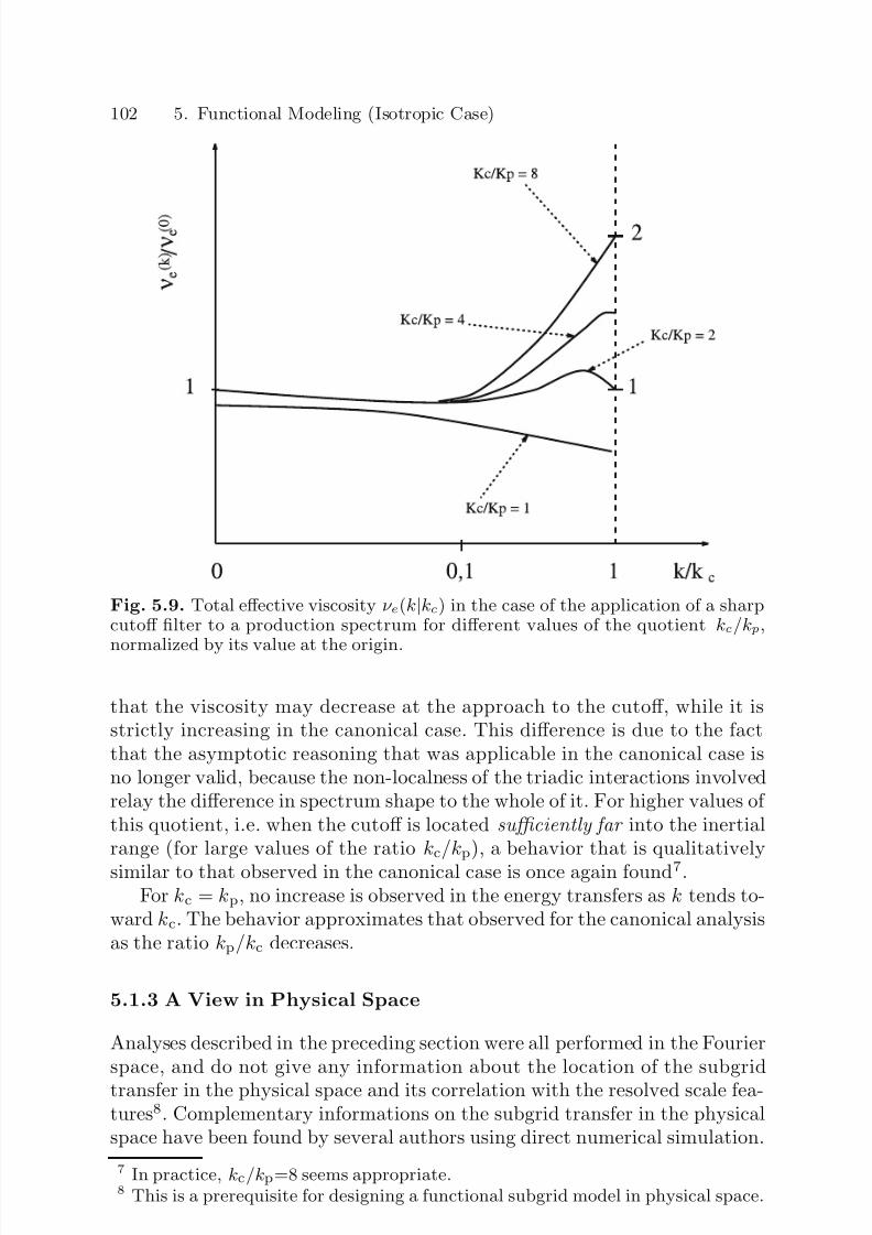
7/21/2019 Large Eddy Simulation for Incompressible Flows
http://slidepdf.com/reader/full/large-eddy-simulation-for-incompressible-flows 124/573
102 5. Functional Modeling (Isotropic Case)
Fig. 5.9. Total effective viscosity ν e(k|kc) in the case of the application of a sharpcutoff filter to a production spectrum for different values of the quotient kc/kp,
normalized by its value at the origin.
that the viscosity may decrease at the approach to the cutoff, while it isstrictly increasing in the canonical case. This difference is due to the factthat the asymptotic reasoning that was applicable in the canonical case isno longer valid, because the non-localness of the triadic interactions involvedrelay the difference in spectrum shape to the whole of it. For higher values of this quotient, i.e. when the cutoff is located sufficiently far into the inertialrange (for large values of the ratio kc/kp), a behavior that is qualitatively
similar to that observed in the canonical case is once again found7.For kc = kp, no increase is observed in the energy transfers as k tends to-
ward kc. The behavior approximates that observed for the canonical analysisas the ratio kp/kc decreases.
5.1.3 A View in Physical Space
Analyses described in the preceding section were all performed in the Fourierspace, and do not give any information about the location of the subgrid
transfer in the physical space and its correlation with the resolved scale fea-tures8. Complementary informations on the subgrid transfer in the physicalspace have been found by several authors using direct numerical simulation.
7 In practice, kc/kp=8 seems appropriate.8 This is a prerequisite for designing a functional subgrid model in physical space.
7/21/2019 Large Eddy Simulation for Incompressible Flows
http://slidepdf.com/reader/full/large-eddy-simulation-for-incompressible-flows 125/573
5.1 Phenomenology of Inter-Scale Interactions 103
Kerr et al. [383] propose to use the rotational form of the non-linear term of the momentum equation:
N (x) = u(x) × ω(x) − ∇ ph(x) , (5.13)
where ω = ∇ × u and ph the pressure term. By splitting the velocity andvorticity field into a resolved and a subgrid contribution, we get:
u × ω − u × ω I
= u × ω II
+ u × ω III
+ u × ω IV
. (5.14)
The four terms represent different coupling mechanisms between the re-
solved motion and the subgrid scales:– I - exact subgrid term,– II - interaction between resolved velocity and subgrid vorticity,– III - interaction between subgrid velocity and resolved vorticity,– IV - interaction between subgrid velocity and subgrid vorticity.
The corresponding complete non-linear terms N I ,...,N IV are built byadding the specific pressure term. The associated subgrid kinetic energytransfer terms are computed as εl = u · N l. The authors made three sig-
nificant observations for isotropic turbulence:– Subgrid kinetic energy transfer is strongly correlated with the boundaries of
regions of large vorticity production (stretching), i.e. regions where ωiS ijωjis large;
– Term II, u × ω, has a correlation with subgrid non-linear term I up to 0.9.This term dominates the backward energy cascade;
– Up to 90% of the subgrid kinetic energy transfer comes from term III, i.e.from the interaction of subgrid velocity with resolved vorticity. This termmostly contributes to the forward energy cascade.
Additional results of Borue and Orszag [72] show that the subgrid transfertakes place in regions where the vorticity stretching term is positive or in
regions with negative skewness of the resolved strain rate tensor, Tr(S 3
).These authors also found that there is only a very poor local correlationbetween the subgrid transfer τ ijS ij and the local strain S ijS ij , where S ij isthe resolved strain rate tensor.
Horiuti [325, 327] decomposed the subgrid tensor into several contribu-tions,9 and used direct numerical simulation data of isotropic turbulence to
analyze their contributions. A first remark is that the eigenvectors of the to-tal subgrid tensor have a preferred orientation of 42 relative to those of S .Eigenvectors of (S ikS kj − Ω ikΩ kj) are highly aligned with those of S , while
9 This decomposition is discussed in the section devoted to nonlinear models,p. 223.

7/21/2019 Large Eddy Simulation for Incompressible Flows
http://slidepdf.com/reader/full/large-eddy-simulation-for-incompressible-flows 126/573
104 5. Functional Modeling (Isotropic Case)
those of (S ikΩ kj − S ikΩ kj) exhibit a 42 angle, from which stems the globalobserved difference. The first term is associated with the forward energycascade. The second one makes no contribution to the total production of subgrid kinetic energy, but is relevant to the vortex stretching and the back-ward energy cascade process.10 Similar results were obtained by Meneveauand coworkers [704, 703].
The role of coherent structures in interscale transfer is of major impor-tance in shear flows. Da Silva and Metais [158] carried out an exhaustivestudy in the plane jet case: the most intense forward cascade events occurnear these coherent structures and not randomly in space. The local equilib-rium assumption is observed to hold globally but not locally as most viscousdissipation of subgrid kinetic energy takes place within coherent structure
cores, while forward and backward cascade occur at different locations.
5.1.4 Summary
The different analyses performed in the framework of fully developed isotropicturbulence show that:
1. Interactions between the small and large scales is reflected by two mainmechanisms:
– A drainage of energy from the resolved scales by the subgrid scales(forward energy cascade phenomenon);
– A weak feedback of energy, proportional to k4 to the resolved scales(backward energy cascade phenomenon).
2. The interactions between the subgrid scales and the smallest of the re-solved scales depend on the filter used and on the shape of the spectrum.In certain cases, the coupling with the subgrid scales is strengthenedfor wave numbers close to the cutoff and the energy toward the subgridmodes is intensified.
3. These cascade mechanisms are associated to specific features of the ve-locity and vorticity field in physical space.
5.2 Basic Functional Modeling Hypothesis
All the subgrid models entering into this category make more or less implicituse of the following hypothesis:
Hypothesis 5.1 The action of the subgrid scales on the resolved scales is essentially an energetic action, so that the balance of the energy transfers alone between the two scale ranges is sufficient to describe the action of the subgrid scales.
10 This is an indication that the backward energy cascade is not associated withnegative subgrid viscosity from the theoretical point of view.
7/21/2019 Large Eddy Simulation for Incompressible Flows
http://slidepdf.com/reader/full/large-eddy-simulation-for-incompressible-flows 127/573
5.3 Modeling of the Forward Energy Cascade Process 105
Using this hypothesis as a basis for modeling, then, we neglect a part of theinformation contained in the small scales, such as the structural informationrelated to the anisotropy. As was seen above, the energy transfers betweensubgrid scales and resolved scales mainly exhibit two mechanisms: a forwardenergy transfer toward the subgrid scales and a backward transfer to theresolved scales which, it seems, is much weaker in intensity. All the approachesexisting today for numerical simulation at high Reynolds numbers considerthe energy lost by the resolved scales, while only a few rare attempts havebeen made to consider the backward energy cascade.
Once hypothesis 5.1 is assumed, the modeling consists in modifying thedifferent evolution equations of the system in such a way as to integrate thedesired dissipation or energy production effects into them. To do this, two
different approaches can be found in today’s works:
– Explicit modeling of the desired effects, i.e. including them by adding ad-ditional terms to the equations: the actual subgrid models;
– Implicit inclusion by the numerical scheme used, by arranging it so thetruncation error induces the desired effects.
Let us note that while the explicit approach is what would have to becalled the classical modeling approach, the implicit one appears generallyonly as an a posteriori interpretation of dissipative properties for certainnumerical methods used.
5.3 Modeling of the Forward Energy Cascade Process
This section describes the main functional models of the energy cascade mech-anism. Those derived in the Fourier space, conceived for simulations based onspectral numerical methods, and models derived in the physical space, suited
to the other numerical methods, are presented separately.
5.3.1 Spectral Models
The models belonging to this category are all effective viscosity models draw-ing upon the analyses of Kraichnan for the canonical case presented above.The following models are described:
1. The Chollet–Lesieur model (p. 106) which, based on the results of thecanonical analysis (inertial range of the spectrum with a slope of -5/3,
sharp cutoff filter, no effects associated with a production type spectrum)yields an analytical expression for the effective viscosity as a function of the wave number considered and the cutoff wave number. It will reflectthe local effects at the cutoff, i.e. the increase in the energy transfer to-ward the subgrid scales. This model explicitly brings out a dependency

7/21/2019 Large Eddy Simulation for Incompressible Flows
http://slidepdf.com/reader/full/large-eddy-simulation-for-incompressible-flows 128/573
106 5. Functional Modeling (Isotropic Case)
of the effective viscosity as a function of the kinetic energy at the cutoff.This guarantees that, when all the modes of the exact solution are re-solved, the subgrid model automatically cancels out. The fact that thisinformation is local in frequency allows the model to consider (at leastpartially) the spectral disequilibrium phenomena that occur at the levelof the resolved scales11, though without relaxing the hypotheses underly-ing the canonical analysis. Only the amplitude of the transfers is variable,and not their pre-supposed shape.
2. The effective viscosity model (p. 107), which is a simplification of theprevious one and is based on the same assumptions. The effective vis-cosity is then independent of the wave number and is calculated so as toensure the same average value as the Chollet–Lesieur model. It is simpler
to compute, but does not reflect the local effects at the cutoff.3. The dynamic spectral model (p. 107), which is an extension of the
Chollet–Lesieur model for spectra having a slope different from that of the canonical case (i.e. - 5/3). Richer information is considered here:while the Chollet–Lesieur model is based only on the energy level at thecutoff, the dynamic spectral model also incorporates the spectrum slopeat the cutoff. With this improvement, we can cancel the subgrid model incertain cases for which the kinetic energy at cutoff is non-zero but wherethe kinetic energy transfer to the subgrid modes is zero12. This model
also reflects the local effects at the cutoff. The other basic assumptionsunderlying the Chollet–Lesieur model are maintained.
4. The Lesieur–Rogallo model (p. 108), which computes the intensity of thetransfers by a dynamic procedure. This is an extension of the Chollet–Lesieur model for flows in spectral disequilibrium, as modifications inthe nature of the transfers to the subgrid scales can be considered. Thedynamic procedure consists in including in the model information relativeto the energy transfers at play with the highest resolved frequencies. Theassumptions concerning the filter are not relaxed, though.
5. Models based on the analytical theories of turbulence (p. 108), whichcompute the effective viscosity without assuming anything about thespectrum shape of the resolved scales, are thus very general. On the otherhand, the spectrum shape of the subgrid scales is assumed to be that of a canonical inertial range. These models, which are capable of includingvery complex physical phenomena, require very much more implementa-tion and computation effort than the previous models. The assumptionsconcerning the filter are the same as for the previous models.
Chollet–Lesieur Model. Subsequent to Kraichnan’s investigations, Chol-let and Lesieur [136] proposed an effective viscosity model using the resultsof the EDQNM closure on the canonical case. The full subgrid transfer term
11 This is by their action on the transfers between resolved scales and the variationsinduced on the energy level at cutoff.
12 As is the case, for example, for two-dimensional flows.

7/21/2019 Large Eddy Simulation for Incompressible Flows
http://slidepdf.com/reader/full/large-eddy-simulation-for-incompressible-flows 129/573
5.3 Modeling of the Forward Energy Cascade Process 107
including the backward cascade is written:
T esgs(k
|kc) =
−2k2E (k)ν e(k
|kc) , (5.15)
in which the effective viscosity ν e(k|kc) is defined as the product
ν e(k|kc) = ν +e (k|kc)ν ∞e . (5.16)
The constant term ν ∞e , independent of k, corresponds the asymptoticvalue of the effective viscosity for wave numbers that are small comparedwith the cutoff wave number kc. This value is evaluated using the cutoff energy E (kc):
ν ∞e = 0.441K
−3/20 E (kc)
kc . (5.17)
The function ν e(k|kc) reflects the variations of the effective viscosity inthe proximity of the cutoff. The authors propose the following form, whichis obtained by approximating the exact solution with a law of exponentialform:
ν +e (k|kc) = 1 + 34.59 exp(−3.03kc/k) . (5.18)
This form makes it possible to obtain an effective viscosity that is nearlyindependent of k for wave numbers that are small compared with kc, with
a finite increase near the cutoff. There is a limited inclusion of the backwardcascade with this model: the effective viscosity remains strictly positive for allwave numbers, while the backward cascade is dominant for very small wavenumbers, which would correspond to negative values of the effective viscosity.
Constant Effective Viscosity Model. A simplified form of the effectiveviscosity of (5.16) can be derived independently of the wave number k [440].By averaging the effective viscosity along k and assuming that the subgridmodes are in a state of energy balance, we get:
ν e(k|kc) = ν e = 23
K −3/20
E (kc)kc
. (5.19)
Dynamic Spectral Model. The asymptotic value of the effective viscosity(5.17) has been extended to the case of spectra of slope −m by Metais
and Lesieur [514] using the EDQNM closure. For a spectrum proportional tok−m, m ≤ 3, we get:
ν ∞
e (m) = 0.31
5 − m
m + 1
√ 3
−mK
−3/2
0 E (kc)
kc. (5.20)
For m > 3, the energy transfer cancels out, inducing zero effective viscos-ity. Here, we find a behavior similar to that of two-dimensional turbulence.Extension of this idea in physical space has been derived by Lamballais andhis coworkers [422, 675].
7/21/2019 Large Eddy Simulation for Incompressible Flows
http://slidepdf.com/reader/full/large-eddy-simulation-for-incompressible-flows 130/573
108 5. Functional Modeling (Isotropic Case)
Lesieur–Rogallo Model. By introducing a new filtering level correspond-ing to the wave number km < kc, Lesieur and Rogallo [441] propose a dynamicalgorithm for adapting the Chollet–Lesieur model. The contribution to thetransfer T (k), k < kc, corresponding to the (k, p, q) triads such that p and/orq are in the interval [km, kc], can be computed explicitly by Fourier trans-forms. This contribution is denoted T sub(k|km, kc) and is associated with theeffective viscosity:
ν e(k|km, kc) = −T sub(k|km, kc)
2k2E (k) . (5.21)
The effective viscosity corresponding to the interactions with wave num-
bers located beyond km is the sum:
ν e(k|km) = ν e(k|km, kc) + ν e(k|kc) . (5.22)
This relation corresponds exactly to Germano’s identity and was previ-ously derived by the authors. The two terms ν e(k|km) and ν e(k|kc) are thenmodeled by the Chollet–Lesieur model. We adopt the hypothesis that whenk < km, then k kc, which leads to ν +e (k|kc) = ν +e (0). Relation (5.22) thenleads to the equation:
ν +e (k|km) = ν e(k|km, kc) km
E (km) + ν +e (0)
kmkc
4/3
. (5.23)
The factor ν +e (0) is evaluated by considering that we have the relations
ν +e (k|km) ≈ ν +e (0), ν e(k|km, kc) ≈ ν e(0|km, kc) , (5.24)
for k km, which leads to:
ν +e (0) = ν e(0|km, kc) km
E (km)
1 −
kmkc
4/3−1
. (5.25)
Models Based on Analytical Theories of Turbulence. The effectiveviscosity models presented above are all based on an approximation of theeffective viscosity profile obtained in the canonical case, and are thereforeintrinsically linked to the underlying hypotheses, especially those concerningthe shape of the energy spectrum. One way of relaxing this constraint is to
compute the effective viscosity directly from the computed spectrum usinganalytical theories of turbulence. This approach has been used by Aupoix [24],Chollet [132, 133], and Bertoglio [56, 57, 58].
More recently, following the recommendations of Leslie and Quarini,which are to model the forward and backward cascade mechanisms separately,
7/21/2019 Large Eddy Simulation for Incompressible Flows
http://slidepdf.com/reader/full/large-eddy-simulation-for-incompressible-flows 131/573
5.3 Modeling of the Forward Energy Cascade Process 109
Chasnov [120] in 1991 proposed an effective viscosity model considering onlythe energy draining effects, with the backward cascade being modeled sepa-rately (see Sect. 5.4). Starting with an EDQNM analysis, Chasnov proposescomputing the effective viscosity ν e(k|kc) as:
ν e(k|kc) = 1
2k2
∞kc
dp
p p−k
dqΘkpq
p2
q (xy + z3)E (q ) +
q 2
p (xz + y3)E ( p)
,
(5.26)in which x, y and z are geometric factors associated with the (k, p, q) triadsand Θkpq a relaxation time. These terms are explained in Appendix B. Tocompute this integral, the shape of the energy spectrum beyond the cutoff kc
must be known. As it is not known a priori , it must be specified elsewhere.In practice, Chasnov uses a Kolmogorov spectrum extending from the cut-off to infinity. To simplify the computations, the relation (5.26) is not usedoutside the interval [kc ≤ p ≤ 3kc]. For wave numbers p > 3kc, the followingsimplified asymptotic form already proposed by Kraichnan is used:
ν e(k|kc) = 1
15
∞kc
dpΘkpq
5E ( p) + p
∂E ( p)
∂p
. (5.27)
5.3.2 Physical Space ModelsSubgrid Viscosity Concept. The forward energy cascade mechanism tothe subgrid scales is modeled explicitly using the following hypothesis:
Hypothesis 5.2 The energy transfer mechanism from the resolved to the subgrid scales is analogous to the molecular mechanisms represented by the diffusion term, in which the viscosity ν appears.
This hypothesis is equivalent to assuming that the behavior of the subgridscales is analogous to the Brownian motion superimposed on the motion of the resolved scales. In gaskinetics theory, molecular agitation draws energyfrom the flow by way of molecular viscosity. So the energy cascade mechanismwill be modeled by a term having a mathematical structure similar to thatof molecular diffusion, but in which the molecular viscosity will be replacedby a subgrid viscosity denoted ν sgs. As Boussinesq proposed, this choice of mathematical form of the subgrid model is written:
−∇ · τ d = ∇ ·
ν sgs(∇u + ∇T u)
, (5.28)
in which τ d is the deviator of τ , i.e.:
τ dij ≡ τ ij − 1
3τ kkδ ij . (5.29)
7/21/2019 Large Eddy Simulation for Incompressible Flows
http://slidepdf.com/reader/full/large-eddy-simulation-for-incompressible-flows 132/573
110 5. Functional Modeling (Isotropic Case)
The complementary spherical tensor 13
τ kkδ ij is added to the filtered staticpressure term and consequently requires no modeling. This decomposition isnecessary since the tensor (
∇u +
∇T u) has a zero trace, and we can only
model a tensor that also has a zero trace. This leads to the definition of themodified pressure Π :
Π = p + 1
3τ kk . (5.30)
It is important to note that the modified pressure and filtered pressure p may take very different values when the generalized subgrid kinetic en-ergy becomes large [374]. The closure thus now consists in determining therelation:
ν sgs = N (u) . (5.31)
The use of hypothesis (5.2) and of a model structured as above calls fora few comments.
Obtaining a scalar subgrid viscosity requires the adoption of the followinghypothesis:
Hypothesis 5.3 A characteristic length l0 and a characteristic time t0 are sufficient for describing the subgrid scales.
Then, by dimensional reasoning similar to Prandtl’s, we arrive at:
ν sgs ∝ l20
t0. (5.32)
Models of the form (5.28) are local in space and time, which is a necessityif they are to be used in practice. This local character, similar to that of themolecular diffusion terms, implies [26, 405, 813]:
Hypothesis 5.4 (Scale Separation Hypothesis) There exists a total
separation between the subgrid and resolved scales.
A spectrum verifying this hypothesis is presented in Fig. 5.10.Using L0 and T 0 to denote the characteristic scales, respectively, of the
resolved field in space and time, this hypothesis can be reformulated as:
l0
L0 1,
t0
T 0 1 . (5.33)
This hypothesis is verified in the case of molecular viscosity. The ratio
between the size of the smallest dynamically active scale, ηK, and the meanfree path ξ fp of the molecules of a gas is evaluated as:
ξ fp
ηK Ma
Re1/4 , (5.34)
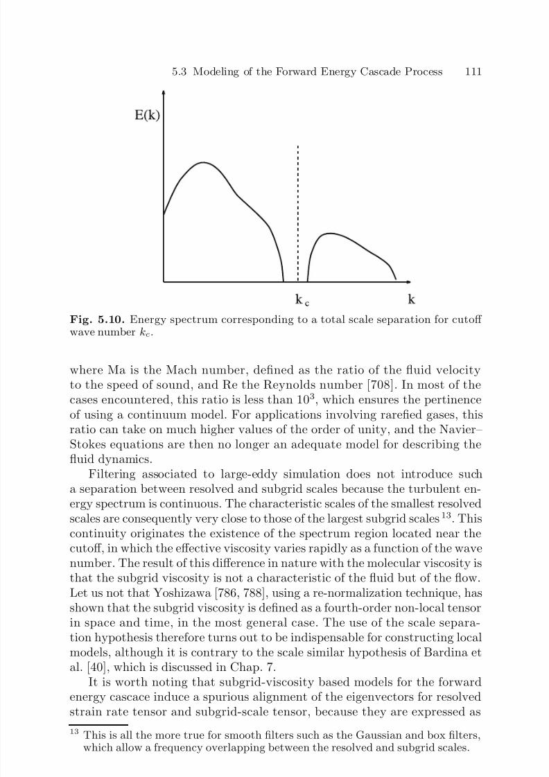
7/21/2019 Large Eddy Simulation for Incompressible Flows
http://slidepdf.com/reader/full/large-eddy-simulation-for-incompressible-flows 133/573
5.3 Modeling of the Forward Energy Cascade Process 111
Fig. 5.10. Energy spectrum corresponding to a total scale separation for cutoff wave number kc.
where Ma is the Mach number, defined as the ratio of the fluid velocityto the speed of sound, and Re the Reynolds number [708]. In most of thecases encountered, this ratio is less than 103, which ensures the pertinenceof using a continuum model. For applications involving rarefied gases, thisratio can take on much higher values of the order of unity, and the Navier–Stokes equations are then no longer an adequate model for describing thefluid dynamics.
Filtering associated to large-eddy simulation does not introduce sucha separation between resolved and subgrid scales because the turbulent en-ergy spectrum is continuous. The characteristic scales of the smallest resolvedscales are consequently very close to those of the largest subgrid scales 13. Thiscontinuity originates the existence of the spectrum region located near the
cutoff, in which the effective viscosity varies rapidly as a function of the wavenumber. The result of this difference in nature with the molecular viscosity isthat the subgrid viscosity is not a characteristic of the fluid but of the flow.Let us not that Yoshizawa [786, 788], using a re-normalization technique, hasshown that the subgrid viscosity is defined as a fourth-order non-local tensorin space and time, in the most general case. The use of the scale separa-tion hypothesis therefore turns out to be indispensable for constructing localmodels, although it is contrary to the scale similar hypothesis of Bardina etal. [40], which is discussed in Chap. 7.
It is worth noting that subgrid-viscosity based models for the forwardenergy cascace induce a spurious alignment of the eigenvectors for resolvedstrain rate tensor and subgrid-scale tensor, because they are expressed as
13 This is all the more true for smooth filters such as the Gaussian and box filters,which allow a frequency overlapping between the resolved and subgrid scales.
7/21/2019 Large Eddy Simulation for Incompressible Flows
http://slidepdf.com/reader/full/large-eddy-simulation-for-incompressible-flows 134/573
112 5. Functional Modeling (Isotropic Case)
τ d ∝ (∇u + ∇T u).14 Tao et al. [703, 704] and Horiuti [325] have shown thatthis alignment is unphysical: the eigenvectors for the subgrid tensor havea strongly preferred relative orientation of 35 to 45 degrees with the resolvedstrain rate eigenvectors.
The modeling problem consists in determining the characteristic scales l0
and t0.
Model Types. The subgrid viscosity models can be classified in three cat-egories according to the quantities they bring into play [26]:
1. Models based on the resolved scales (p. 113): the subgrid viscosity isevaluated using global quantities related to the resolved scales. The ex-istence of subgrid scales at a given point in space and time will therefore
be deduced from the global characteristics of the resolved scales, whichrequires the introduction of assumptions.
2. Models based on the energy at the cutoff (p. 116): the subgrid viscosityis calculated from the energy of the highest resolved frequency. Here, itis a matter of information contained in the resolved field, but localized infrequency and therefore theoretically more pertinent for describing thephenomena at cutoff than the quantities that are global and thus notlocalized in frequency, which enter into the models of the previous class.The existence of subgrid scales is associated with a non-zero value of the
energy at cutoff 15
.3. Models based on the subgrid scales (p. 116), which use information di-
rectly related to the subgrid scales. The existence of the subgrid scales isno longer determined on the basis of assumptions concerning the char-acteristics of the resolved scales as it is in the previous cases, but ratherdirectly from this additional information. These models, because they arericher, also theoretically allow a better description of these scales thanthe previous models.
These model classes are presented in the following. All the developments
are based on the analysis of the energy transfers in the canonical case. Inorder to be able to apply the models formulated from these analyses to morerealistic flows, such as the homogeneous isotropic flows associated with a pro-duction type spectrum, we adopt the assumption that the filter cutoff fre-
14 But it must be also remembered that the purpose of these functional modelsis not to predict the subgrid tensor, but just to enforce the correct resolvedkinetic energy balance. This reconstruction of the subgrid tensor is nothing butan a posteriori interpretation. This fact is used by Germano to derive new subgridviscosity models [252].
15
This hypothesis is based on the fact that the energy spectrum E (k) of an isotropicturbulent flow in spectral equilibrium corresponding to a Kolmogorov spectrumis a monotonic continuous decreasing function of the wave number k. If thereexists a wave number k∗ such that E (k∗) = 0, then E (k) = 0, ∀k > k∗. Also, if the energy is non-zero at the cutoff, then subgrid modes exist, i.e. if E (kc) = 0,then there exists a neighbourhood Ω kc = [kc, kc + c], c > 0 such that E (kc) ≥E (k) ≥ 0 ∀k ∈ Ω kc .

7/21/2019 Large Eddy Simulation for Incompressible Flows
http://slidepdf.com/reader/full/large-eddy-simulation-for-incompressible-flows 135/573
5.3 Modeling of the Forward Energy Cascade Process 113
quency is located sufficiently far into the inertial range for these analyses toremain valid (refer to Sect. 5.1.2). The use of these subgrid models for arbi-trary developed turbulent flows (anisotropic, inhomogeneous) is justified bythe local isotropy hypothesis: we assume then that the cutoff occurs in thescale range that verifies this hypothesis.
The case corresponding to an isotropic homogeneous flow associated witha production spectrum is represented in Fig. 5.11. Three energy fluxes aredefined: the injection rate of turbulent kinetic energy into the flow by thedriving mechanisms (forcing, instabilities), denoted εI ; the kinetic energytransfer rate through the cutoff, denoted
ε; and the kinetic energy dissipation
rate by the viscous effects, denoted ε.
Models Based on the Resolved Scales. These models are of the generic form:
ν sgs = ν sgs
∆, ε
, (5.35)
in which ∆ is the characteristic cutoff length of the filter and ε the instan-taneous energy flux through the cutoff. We implicitly adopt the assumptionhere, then, that the subgrid modes exist, i.e. that the exact solution is notentirely represented by the filtered field when this flux is non-zero.
First Method. Simple dimensional analysis shows that:
ν sgs ∝ ε1/3 ∆4/3
. (5.36)
Fig. 5.11. Dynamics of the kinetic energy in the spectral space. The energy isinjected at the rate εI . The transfer rate through the cutoff, located wave numberkc, is denoted ε. The dissipation rate due to viscous effects is denoted ε. The localequilibrium hypothesis is expressed by the equality εI = ε = ε.
7/21/2019 Large Eddy Simulation for Incompressible Flows
http://slidepdf.com/reader/full/large-eddy-simulation-for-incompressible-flows 136/573
114 5. Functional Modeling (Isotropic Case)
Reasoning as in the framework of Kolmogorov’s hypotheses for isotropichomogeneous turbulence, for the case of an infinite inertial spectrum of theform
E (k) = K 0 ε2/3k−5/3, K 0 ∼ 1.4 , (5.37)
in which ε is the kinetic energy dissipation rate, we get the equation:
ν sgs = A
K 0π4/3ε1/3 ∆
4/3, (5.38)
in which the constant A is evaluated as A = 0.438 with the TFM modeland as A = 0.441 by the EDQNM theory [26]. The angle brackets operator
, designates a statistical average. This statistical averaging operation is
intrinsically associated with a spatial mean by the fact of the flow’s spatialhomogeneity and isotropy hypotheses. This notation is used in the followingto symbolize the fact that the reasoning followed in the framework of isotropichomogeneous turbulence applies only to the statistical averages and not tothe local values in the physical space. The problem is then to evaluate theaverage flux ε. In the isotropic homogeneous case, we have:
2|S |2 = 2S ijS ij =
kc
0
2k2E (k)dk, kc = π
∆. (5.39)
If the cutoff kc is located far enough into the inertial range, the aboverelation can be expressed solely as a function of this region’s characteristicquantities. Using a spectrum of the shape (5.37), we get:
2|S |2 = π4/3K 03
2ε2/3 ∆
−4/3. (5.40)
Using the hypothesis16 [447]:
|S |3/2
|S |3/2
, (5.41)
we get the equality:
ε = 1
π2
3K 0
2
−3/2
∆22|S |23/2 . (5.42)
In order to evaluate the dissipation rate ε from the information con-tained in the resolved scales, we assume the following:
Hypothesis 5.5 (Local Equilibrium Hypothesis) The flow is in con-stant spectral equilibrium, so there is no accumulation of energy at any fre-quency and the shape of the energy spectrum remains invariant with time.
16 The error margin measured in direct numerical simulations of isotropic homoge-neous turbulence is of the order of 20% [507].
7/21/2019 Large Eddy Simulation for Incompressible Flows
http://slidepdf.com/reader/full/large-eddy-simulation-for-incompressible-flows 137/573
5.3 Modeling of the Forward Energy Cascade Process 115
This implies an instantaneous adjustment of all the scales of the solutionto the turbulent kinetic energy production mechanism, and therefore equalitybetween the production, dissipation, and energy flux through the cutoff:
εI = ε = ε . (5.43)
Using this equality and relations (5.38) and (5.42), we get the closurerelation:
ν sgs =
C∆2 2|S |21/2 , (5.44)
where the constant C is evaluated as:
C =
√ A
π√ K 0 3K 02 −1/4
∼ 0.148 . (5.45)
Second Method. The local equilibrium hypothesis allows:
ε = ε ≡ −S ijτ ij = ν sgs2S ijS ij . (5.46)
The idea is then to assume that:
ν sgs2S ijS ij = ν sgs2S ijS ij . (5.47)
By stating at the outset that the subgrid viscosity is of the form (5.44)and using relation (5.40), a new value is found for the constant C :
C = 1
π
3K 0
2
−3/4
∼ 0.18 . (5.48)
We note that the value of this constant is independent of the cutoff wavenumber kc, but because of the way it is calculated, we can expect a depen-dency as a function of the spectrum shape.
Alternate Form. This modeling induces a dependency as a function of thecutoff length ∆ and the strain rate tensor S of the resolved velocity field. Inthe isotropic homogeneous case, we have the equality:
2|S |2 = ω · ω, ω = ∇ × u . (5.49)
By substitution, we get the equivalent form [487]:
ν sgs = C∆2 ω · ω1/2 . (5.50)
These two versions bring in the gradients of the resolved velocity field.This poses a problem of physical consistency since the subgrid viscosity isnon-zero as soon as the velocity field exhibits spatial variations, even if it islaminar and all the scales are resolved. The hypothesis that links the existenceof the subgrid modes to that of the mean field gradients therefore prevents
7/21/2019 Large Eddy Simulation for Incompressible Flows
http://slidepdf.com/reader/full/large-eddy-simulation-for-incompressible-flows 138/573
116 5. Functional Modeling (Isotropic Case)
us from considering the large scale intermittency and thereby requires usto develop models which by nature can only be effective for dealing withflows that are completely turbulent and under-resolved everywhere17. Poorbehavior can therefore be expected when treating intermittent or weaklydeveloped turbulent flows (i.e. in which the inertial range does not appear inthe spectrum) due to too strong an action by the model.
Models Based on the Energy at Cutoff. The models of this category are basedon the intrinsic hypothesis that if the energy at the cutoff is non-zero, thensubgrid modes exist.
First Method. Using relation (5.38) and supposing that the cutoff occurswithin an inertial region, i.e.:
E (kc) = K 0 ε2/3 k−5/3c , (5.51)
by substitution, we get:
ν sgs = A√
K 0
E (kc)
kc, kc = π/∆ . (5.52)
This model raises the problem of determining the energy at the cutoff
in the physical space, but on the other hand ensures that the subgrid vis-cosity will be null if the flow is well resolved, i.e. if the highest-frequencymode captured by the grid is zero. This type of model thus ensures a betterphysical consistency than those models based on the large scales. It shouldbe noted that it is equivalent to the spectral model of constant effective vis-cosity.
Second Method. As in the case of models based on the large scales, thereis a second way of determining the model constant. By combining rela-tions (5.46) and (5.51), we get:
ν sgs = 2
3K 3/20
E (kc)
kc. (5.53)
Models Based on Subgrid Scales. Here we considers models of the form:
ν sgs = ν sgs
∆, q 2sgs, ε , (5.54)
in which q 2sgs is the kinetic energy of the subgrid scales and ε the kinetic
energy dissipation rate18
. These models contain more information about the17 In the sense that the subgrid modes exist at each point in space and at each time
step.18 Other models are of course possible using other subgrid scale quantities like
a length or time scale, but we limit ourselves here to classes of models for whichpractical results exist.

7/21/2019 Large Eddy Simulation for Incompressible Flows
http://slidepdf.com/reader/full/large-eddy-simulation-for-incompressible-flows 139/573
5.3 Modeling of the Forward Energy Cascade Process 117
subgrid modes than those belonging to the two categories described above,and thereby make it possible to do without the local equilibrium hypothe-sis (5.5) by introducing characteristic scales specific to the subgrid modes byway of q 2sgs and ε. This capacity to handle the energy disequilibrium isexpressed by the relation:
ε ≡ −τ ijS ij = ε , (5.55)
which should be compared with (5.43). In the case of an inertial range ex-tending to infinity beyond the cutoff, we have the relation:
q 2sgs ≡
1
2 uiui = ∞kc
E (k)dk =
3
2 K 0ε2/3
k−2/3c , (5.56)
from which we deduce:
ε = kc
(3K 0/2)3/2q 2sgs3/2 . (5.57)
By introducing this last equation into relation (5.38), we come to thegeneral form:
ν sgs = C αεα/3q 2sgs(1−α)/2∆1+α/3 , (5.58)
in which
C α = A
K 0π4/3
3K 0
2
(α−1)/2
π(1−α)/3 , (5.59)
and in which α is a real weighting parameter. Interesting forms of ν sgs havebeen found for certain values:
– For α = 1, we get
ν sgs = A
K 0π4/3∆
4/3ε1/3 . (5.60)
This form uses only the dissipation and is analogous to that of the modelsbased on the resolved scales. If the local equilibrium hypothesis is used,these two types of models are formally equivalent.
– For α = 0, we get
ν sgs = 23
AπK
3/20
∆ q 2sgs1/2 . (5.61)
This model uses only the kinetic energy of the subgrid scales. As such,it is formally analogous to the definition of the diffusion coefficient of anideal gas in the framework of gaskinetics theory. In the case of an inertial
7/21/2019 Large Eddy Simulation for Incompressible Flows
http://slidepdf.com/reader/full/large-eddy-simulation-for-incompressible-flows 140/573
118 5. Functional Modeling (Isotropic Case)
spectrum extending to infinity beyond the cutoff, this model is strictlyequivalent to the model based on the energy at cutoff, since in this precisecase we have the relation:
3
2kcE (kc) = q 2sgs . (5.62)
– For α = −3, we have:
ν sgs = 4A
9K 30
q 2sgs2
ε . (5.63)
This model is formally analogous to the k−ε statistical model of turbulence
for the Reynolds Averaged Navier–Stokes equations, and does not bring inthe filter cutoff length explicitly.
The closure problem consists in determining the quantities ε and q 2sgs.To do this, we can introduce one or more equations for the evolution of these quantities or we can deduce them from the information contained inthe resolved field. As these quantities represent the subgrid scales, we are
justified in thinking that, if they are correctly evaluated, the subgrid viscositywill be negligible when the flow is well resolved numerically. However, itshould be noted that these models in principle require more computation than
those based on the resolved scales, because they produce more informationconcerning the subgrid scales.
Extension to Other Spectrum Shapes. The above developments are based ona Kolmogorov spectrum, which reflects only the existence of a region of sim-ilarity of the real spectra. This approach can be extended to other morerealistic spectrum shapes, mainly including the viscous effects. Several ex-tensions of the models based on the large scales were proposed by Voke [737]for this. The total dissipation ε can be decomposed into the sum of thedissipation associated with the large scales, denoted
ε
r, and the dissipation
associated with the subgrid scales, denoted εsgs, (see Fig. 5.12):
ε = εr + εsgs . (5.64)
These three quantities can be evaluated as:
ε = 2(ν sgs + ν )|S |2 , (5.65)
εr = 2ν |S |2 = 2ν
kc
0
k2E (k)dk , (5.66)
εsgs = 2ν sgs|S |2 = C s∆2 2|S |23/2 , (5.67)
from which we get:
εrε =
1
1 + ν , ν =
ν sgsν
. (5.68)

7/21/2019 Large Eddy Simulation for Incompressible Flows
http://slidepdf.com/reader/full/large-eddy-simulation-for-incompressible-flows 141/573
5.3 Modeling of the Forward Energy Cascade Process 119
Fig. 5.12. Kinetic energy dynamics in the spectral space. The energy is injectedat the rate εI . The transfer rate through the cutoff located at the wave numberkc is denoted ε. The dissipation rate in the form of heat by the viscous effectsassociated with the scales located before and after the cutoff kc are denoted εr andεsgs, respectively.
This ratio is evaluated by calculating the εr term analytically from thechosen spectrum shapes, which provides a way of then computing the subgridviscosity ν sgs.
We define the three following parameters:
κ = k
kd= k
ν 3
ε1/4
, κc = kc
kd, (5.69)
Re∆ =∆
2 2|S |2
ν , (5.70)
in which kd is the wave number associated with the Kolmogorov scale (seeAppendix A), and Re∆ is the mesh-Reynolds number. Algebraic substitutionslead to:
κ = πRe−1/2
∆ (1 + ν )−1/4 . (5.71)
The spectra studied here are of the generic form:
E (k) = K 0ε2/3k−5/3f (κ) , (5.72)
in which f is a damping function for large wave numbers. The following aresome commonly used forms of this function:
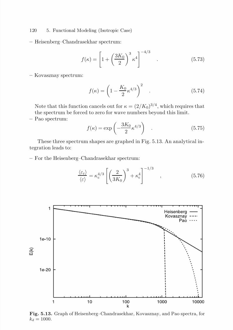
7/21/2019 Large Eddy Simulation for Incompressible Flows
http://slidepdf.com/reader/full/large-eddy-simulation-for-incompressible-flows 142/573
120 5. Functional Modeling (Isotropic Case)
– Heisenberg–Chandrasekhar spectrum:
f (κ) = 1 + 3K 02 3
κ4−4/3
. (5.73)
– Kovasznay spectrum:
f (κ) =
1 − K 0
2 κ4/3
2
. (5.74)
Note that this function cancels out for κ = (2/K 0)3/4, which requires thatthe spectrum be forced to zero for wave numbers beyond this limit.
– Pao spectrum:
f (κ) = exp
−3K 0
2 κ4/3
. (5.75)
These three spectrum shapes are graphed in Fig. 5.13. An analytical in-tegration leads to:
– For the Heisenberg–Chandrasekhar spectrum:
εrε = κ4/3c 2
3K 03
+ κ4c−1/3
, (5.76)
Fig. 5.13. Graph of Heisenberg–Chandrasekhar, Kovasznay, and Pao spectra, forkd = 1000.
7/21/2019 Large Eddy Simulation for Incompressible Flows
http://slidepdf.com/reader/full/large-eddy-simulation-for-incompressible-flows 143/573
5.3 Modeling of the Forward Energy Cascade Process 121
or:
ν sgs = ν κ
−4/3
c 2
3K 03
+ κ4
c1/3
− 1 . (5.77)
– For the Kovazsnay spectrum:
εrε = 1 −
1 − K 0
2 κ4/3
c
3
, (5.78)
or:
ν sgs = ν 1 − 1 − K 02
κ4/3c3−1
− 1 . (5.79)
– For the Pao spectrum:
εrε = 1 − exp
3K 0
2 κ4/3
c
3
, (5.80)
or:
ν sgs = ν
1 − exp
3K 0
2 κ4/3
c
3−1
− 1
. (5.81)
These new estimates of the subgrid viscosity ν sgs make it possible totake the viscous effects into account, but requires that the spectrum shapebe set a priori , as well as the value of the ratio κc between the cutoff wavenumber kc and the wave number kd associated with the Kolmogorov scale.
Inclusion of the Local Effects at Cutoff. The subgrid viscosity models in thephysical space, such as they have been developed, do not reflect the increase inthe coupling intensity with the subgrid modes when we consider modes nearthe cutoff. These models are therefore analogous to that of constant effectiveviscosity. To bring out these effects in the proximity of the cutoff, Chol-let [134], Ferziger [217], Lesieur and Metais [440], Deschamps [176], Borueand Orszag [68, 69, 70, 71], Winckelmans and co-workers [762, 163, 759] andLayton [427] propose introducing high-order dissipation terms that will havea strong effect on the high frequencies of the resolved field without affectingthe low frequencies.
Chollet [134], when pointing out that the energy transfer term T esgs canbe written in the general form
T esgs(k|kc) = −2ν (n)e (k|kc)k2nE (k) , (5.82)
7/21/2019 Large Eddy Simulation for Incompressible Flows
http://slidepdf.com/reader/full/large-eddy-simulation-for-incompressible-flows 144/573
122 5. Functional Modeling (Isotropic Case)
in which ν (n)e (k|kc) is a hyper-viscosity, proposes modeling the subgrid term
in the physical space as the sum of an ordinary subgrid viscosity model anda sixth-order dissipation. This new model is expressed:
∇ · τ = −ν sgs
C 1∇2 + C 2∇6
u , (5.83)
in which C 1 and C 2 are constants. Ferziger proposes introducing a fourth-order dissipation by adding to the subgrid tensor τ the tensor τ (4), definedas:
τ (4)ij =
∂
∂xj
ν (4)
sgs
∂ 2ui∂xk∂xk
+
∂
∂xi
ν (4)
sgs
∂ 2uj∂xk∂xk
, (5.84)
or as
τ (4)ij =
∂ 2
∂xk∂xk
ν (4)
sgs
∂ui∂xj
+ ∂uj∂xi
, (5.85)
in which the hyper-viscosity ν (4)sgs is defined by dimensional arguments as
ν (4)sgs = C m∆
4|S | . (5.86)
The full subgrid term that appears in the momentum equations is thenwritten:
τ ij = τ (2)ij + τ (4)ij , (5.87)
in which τ (2)ij is a subgrid viscosity model described above. A similar form is
proposed by Lesieur and Metais: after defining the velocity field u as
u = ∇2 pu , (5.88)
the two authors propose the composite form:
τ ij =−
ν sgsS ij + (−
1) p+1ν
sgs
S
ij
, (5.89)
in which ν sgs hyper-viscosity obtained by applying a subgrid viscosity modelto the u field, and S the strain rate tensor computed from this same field.The constant of the subgrid model used should be modified to verify the localequilibrium relation, which is
−τ ijS ij = ε .
This composite form of the subgrid dissipation has been validated exper-
imentaly by Cerutti et al. [115], who computed the spectral distribution of dissipation and the corresponding spectral viscosity from experimental data.It is worth noting that subgrid dissipations defined thusly, as the sum of
second- and fourth-order dissipations, are similar in form to certain numeri-cal schemes designed for capturing strong gradients, like that of Jameson etal. [346].

7/21/2019 Large Eddy Simulation for Incompressible Flows
http://slidepdf.com/reader/full/large-eddy-simulation-for-incompressible-flows 145/573
5.3 Modeling of the Forward Energy Cascade Process 123
Borue and Orszag [68, 69, 70, 71] propose to eliminate the molecular andthe subgrid viscosities by replacing them by a higher power of the Laplacianoperator. Numerical tests show that three-dimensional inertial-range dynam-ics is relatively independent of the form of the hyperviscosity. It was alsoshown that for a given numerical resolution, hyperviscous dissipations in-crease the extent of the inertial range of three-dimensional turbulence by anorder of magnitude. It is worth noting that this type of iterated Laplacianis commonly used for two-dimensional simulations. Borue and Orszag useda height-time iterated Laplacian to get these conclusions. Such operators areeasily defined when using spectral methods, but are of poor interest whendealing with finite difference of finite volume techniques.
Subgrid-Viscosity Models. Various subgrid viscosity models belongingto the three categories defined above will now be described. These are thefollowing:
1. The Smagorinsky model (p. 124), which is based on the resolved scales.This model, though very simple to implant, suffers from the defects al-ready mentioned for the models based on the large scales.
2. The second-order Structure Function model developed by Metais andLesieur (p. 124), which is an extension into physical space of the mod-els based on the energy at cutoff. Theoretically based on local frequency
information, this model should be capable of treating large-scale inter-mittency better than the Smagorinsky model. However, the impossibilityof localizing the information in both space and frequency (see discussionfurther on) reduces its efficiency.
3. The third-order Structure Function models developed by Shao (p. 126),which can be interpreted as an extension of the previous model basedon the second-order structure function. The use of the Kolmogorov–Meneveau equation [510] for the filtered third-order structure functionenables the definition of several models which do not contain arbitrary
constants and have improved potentiality for non-equilibrium flows.4. A model based on the kinetic energy of the subgrid modes (p. 128). This
energy is considered as an additional variable of the problem, and isevaluated by solving an evolution equation. Since it contains informationrelative to the subgrid scales, it is theoretically more capable of handlinglarge-scale intermittency than the previous model. Moreover, the localequilibrium hypothesis can be relaxed, so that the spectral nonequilib-rium can be integrated better. The model requires additional hypotheses,though (modeling, boundary conditions).
5. The Yoshizawa model (p. 129), which includes an additional evolutionequation for a quantity linked to a characteristic subgrid scale, by whichit can be classed among models based on the subgrid scales. It has thesame advantages and disadvantages as the previous model.
6. The Mixed Scale Model (p. 130), which uses information related both tothe subgrid modes and to the resolved scales, though without incorpo-
7/21/2019 Large Eddy Simulation for Incompressible Flows
http://slidepdf.com/reader/full/large-eddy-simulation-for-incompressible-flows 146/573
124 5. Functional Modeling (Isotropic Case)
rating additional evolution equations. The subgrid scale data is deducedfrom that contained in the resolved scales by extrapolation in the fre-quency domain. This model is of intermediate level of complexity (andquality) between those based on the large scales and those that use ad-ditional variables.
Smagorinsky Model. The Smagorinsky model [676] is based on the largescales. It is generally used in a local form the physical space, i.e. variablein space, in order to be more adaptable to the flow being calculated. It isobtained by space and time localization of the statistical relations given inthe previous section. There is no particular justification for this local useof relations that are on average true for the whole, since they only ensure
that the energy transfers through the cutoff are expressed correctly on theaverage, and not locally.
This model is expressed:
ν sgs(x, t) =
C s∆2
(2|S (x, t)|2)1/2 . (5.90)
The constant theoretical value C s is evaluated by the relations (5.45)or (5.48). It should nonetheless be noted that the value of this constant is,in practice, adjusted to improve the results. Clark et al. [143] use C s = 0.2
for a case of isotropic homogeneous turbulence, while Deardorff [172] usesC s = 0.1 for a plane channel flow. Studies of shear flows using experimentaldata yield similar evaluations (C s 0.1 − 0.12) [503, 570, 724]. This decreasein the value of the constant with respect to its theoretical value is due tothe fact that the field gradient is now non-zero and that it contributes tothe |S (x, t)| term. To enforce the local equilibrium relation, the value of theconstant has to be reduced. It should be noted that this new value ensuresonly that the right quantity of resolved kinetic energy will be dissipated onthe whole throughout the field, but that the quality of the level of local
dissipation is uncontrolled. 19
Second-Order Structure Function Model. This model is a transpositionof Metais and Lesieur’s constant effective viscosity model into the physicalspace, and can consequently be interpreted as a model based on the energyat cutoff, expressed in physical space. The authors [514] propose evaluatingthe energy at cutoff E (kc) by means of the second-order velocity structure
19 Canuto and Cheng [99] derived a more general expression for the constant C s,which appears as an explicit function of the subgrid kinetic energy and the localshear:
C s ∝
q 2sgs
ε|S |∆2
1/2
,
which is effectively a decreasing function of the local shear |S |. That demonstratesthe limited theoretical range of application of the usual Smagorinsky model.
7/21/2019 Large Eddy Simulation for Incompressible Flows
http://slidepdf.com/reader/full/large-eddy-simulation-for-incompressible-flows 147/573
5.3 Modeling of the Forward Energy Cascade Process 125
function. This is defined as:
DLL(x, r, t) = |x|=r [u(x, t) − u(x + x
, t)]
2
d
3
x
. (5.91)
In the case of isotropic homogeneous turbulence, we have the relation:
DLL(r, t) =
DLL(x, r, t)d3x = 4
∞0
E (k, t)
1 − sin(kr)
kr
dk . (5.92)
Using a Kolmogorov spectrum, the calculation of (5.92) leads to:
DLL(r, t) = 95 Γ (1/3)K 0ε2/3r2/3 , (5.93)
or, expressing the dissipation ε, as a function of DLL(r, t) in the expressionfor the Kolmogorov spectrum:
E (k) = 5
9Γ (1/3)DLL(r, t)r−2/3k−5/3 . (5.94)
To derive a subgrid model, we now have to evaluate the second-order
structure function from the resolved scales alone. To do this, we decomposeby:
DLL(r, t) = DLL(r, t) + C 0(r, t) , (5.95)
in which DLL(r, t) is computed from the resolved scales and C 0(r, t) corre-sponds to the contribution of the subgrid scales:
C 0(r, t) = 4
∞kc
E (k, t)
1 − sin(kr)
kr
dk . (5.96)
By replacing the quantity E (k, t) in equation (5.96) by its value (5.94),we get:
C 0(r, t) = DLL(r, t)
r
∆
−2/3
H sf (r/∆) , (5.97)
in which H sf is the function
H sf (x) = 20
9Γ (1/3) 3
2π2/3 + x2/3Im exp(ı5π/6)Γ (−5/3,ıπx)
. (5.98)
Once it is substituted in (5.95), this equation makes it possible to evaluatethe energy at the cutoff. The second-order Structure Function model takesthe form:
ν sgs(r) = A(r/∆)∆
DLL(r, t) , (5.99)
7/21/2019 Large Eddy Simulation for Incompressible Flows
http://slidepdf.com/reader/full/large-eddy-simulation-for-incompressible-flows 148/573
126 5. Functional Modeling (Isotropic Case)
in which
A(x) =
2K −3/20
3π4/3 (9/5)Γ (1/3)x−4/3 1 − x
−2/3
H sf (x)−1/2
. (5.100)
In the same way as for the Smagorinsky model, a local model in spacecan be had by using relation (5.94) locally in order to include the local inter-mittency of the turbulence. The model is then written:
ν sgs(x, r) = A(r/∆)∆
DLL(x, r, t) . (5.101)
In the case where r = ∆, the model takes the simplified form:
ν sgs(x, ∆ , t) = 0.105∆
DLL(x, ∆ , t) . (5.102)
A link can be established with the models based on the resolved scalegradients by noting that:
u(x, t) − u(x + x, t) = −x · ∇u(x, t) + O(|x|2) . (5.103)
This last relation shows that the function F 2 is homogeneous to a norm of
the resolved velocity field gradient. If this function is evaluated in the simula-tion in a way similar to how the resolved strain rate tensor is computed for theSmagorinsky model, we can in theory expect the Structure Function model tosuffer some of the same weaknesses: the information contained in the modelwill be local in space, therefore non-local in frequency, which induces a poorestimation of the kinetic energy at cutoff and a loss of precision of the modelin the treatment of large-scale intermittency and spectral nonequilibrium.
Third-Order Structure Functions Models. Shao et al. [669, 153] defineda more general class of structure function-based subgrid viscosities consider-
ing the Kolmogorov–Meneveau equation for the third-order velocity structurefunction in isotropic turbulence [510]
−4
5rε = DLLL − 6GLLL , (5.104)
where DLLL is the third-order longitudinal velocity correlation of the filteredfield
DLLL(r) = [u(x + r) − u(x)]3 , (5.105)
where · denotes the statistical average operator (which is equivalent to theintegral sequence introduced in the presentation of the second-order structurefunction model). The two other quantities are the longitudinal velocity-stresscorrelation tensor
GLLL(r) = u1(x)τ 11(x + r) , (5.106)
7/21/2019 Large Eddy Simulation for Incompressible Flows
http://slidepdf.com/reader/full/large-eddy-simulation-for-incompressible-flows 149/573
5.3 Modeling of the Forward Energy Cascade Process 127
and the average subgrid dissipation
ε =
−τ ijS ij . (5.107)
Shao’s procedure consists in using relation (5.104) to compute the subgridviscosity. To this end, he assumes that the velocity-stress correlation obeysthe following scale-similarity hypothesis
GLLL(r) ∝ r p , (5.108)
where p = −1/3 corresponds to the Kolmogorov local isotropy hypotheses.Using that assumption, one obtains the following relationship for two space
increments r1 and r2:
0.8r1ε + DLLL(r1)
0.8r2ε + DLLL(r2)=
r1
r2
−1/3
. (5.109)
Now introducing a subgrid viscosity model with subgrid viscosity ν sgs,several possibilities exist for the evaluation of the subgrid viscosity. The threefollowing models have been proposed by Shao and his coworkers:
– The one-scale, constant subgrid viscosity model . Assuming that the subgrid
viscosity is constant, one obtains
τ ij = −2ν sgsS ij , ε = ν sgs|S |2, GLLL = ν sgsDLL,r , (5.110)
where comma separated indices denote derivatives. Inserting these relationsinto (5.104), an expression for the eddy viscosity is recovered:
ν sgs = −S k
0.8 |S |2
DLL− 4
r
DLL , (5.111)
where the skewness of the longitudinal filtered velocity increment is definedas
S k = DLLL
D3/2LL
. (5.112)
The Metais-Lesieur model is recovered taking r = ∆ and using propertiesof isotropic turbulence to evaluate the different terms appearing in (5.111).
– The one-scale, variable subgrid viscosity model . Relaxing the previous con-
traint dealing with the constant appearing in the structure-function model,one obtains the following asymptotic expression
ν sgs = −S k
8 r
DLL . (5.113)
7/21/2019 Large Eddy Simulation for Incompressible Flows
http://slidepdf.com/reader/full/large-eddy-simulation-for-incompressible-flows 150/573
128 5. Functional Modeling (Isotropic Case)
The constant is observed to be self-adpative, depending on the computedvalue of the skewness parameter S k.
– The multiscale structure function model . The last model derived by Shaois more general and is based on the two-scale relation (5.109). Using therelation ε = ν sgs|S |2 and considering two diffrent separation distances r1
and r2, one obtain the following expression
ν sgs =DLLL(r1) −
r1r2
1/3
DLLL(r2)
−0.4|S |2
1 −
r1r2
4/3
r1
. (5.114)
These expressions are made local in the physical space by using localvalues of the different parameters involving the resolved velocity field u.
Model Based on the Subgrid Kinetic Energy. One model, of theform (5.61), based on the subgrid scales, was developed independently bya number of authors [318, 653, 791, 792, 525, 690, 391]. The subgrid viscosityis computed from the kinetic energy of the subgrid modes q 2sgs:
ν sgs(x, t) = C m∆
q 2sgs(x, t) , (5.115)
where, for reference:
q 2sgs(x, t) = 1
2(ui(x, t) − ui(x, t))2 . (5.116)
The constant C m is evaluated by the relation (5.61). This energy consti-tutes another variable of the problem and is evaluated by solving an evolutionequation. This equation is obtained from the exact evolution equation (3.33),whose unknown terms are modeled according to Lilly’s proposals [447], or bya re-normalization method. The various terms are modeled as follows (referto the work of McComb [464], for example):
– The diffusion term is modeled by a gradient hypothesis, by stating thatthe non-linear term is proportional to the kinetic energy q 2sgs gradient(Kolmogorov-Prandtl relation):
∂
∂xj 1
2uiu
iuj + uj p
= C 2
∂
∂xj
∆
q 2sgs
∂q 2sgs
∂xj
. (5.117)
– The dissipation term is modeled using dimensional reasoning, by:
ε = ν
2
∂ui∂xj
∂ui∂xj
= C 1(q 2sgs)
3/2
∆. (5.118)
7/21/2019 Large Eddy Simulation for Incompressible Flows
http://slidepdf.com/reader/full/large-eddy-simulation-for-incompressible-flows 151/573
5.3 Modeling of the Forward Energy Cascade Process 129
The resulting evolution equation is:
∂q 2sgs
∂t +∂ujq 2
sgs∂xj I
= −τ ijS ij II
− C 1q 2
sgs
3/2
∆ III
+ C 2∂
∂xj
∆
q 2sgs
∂q 2sgs
∂xj
IV
+ ν ∂ 2q 2sgs
∂xj∂xj V
, (5.119)
in which C 1 and C 2 are two positive constants and the various terms repre-sent:
– I - advection by the resolved modes,– II - production by the resolved modes,– III - turbulent dissipation,– IV - turbulent diffusion,– V - viscous dissipation.
Using an analytical theory of turbulence, Yoshizawa [791, 792] and Ho-riuti [318] propose C 1 = 1 and C 2 = 0.1.
Yoshizawa Model. The filter cutoff length, ∆, is the only length scaleused in deriving models based on the large scales, as this derivation hasbeen explained above. The characteristic length associated with the subgridscales, denoted ∆f , is assumed to be proportional to this length, and thedevelopments of Sect. 5.3.2 show that:
∆f = C s∆ . (5.120)
The variations in the structure of the subgrid modes cannot be included
by setting a constant value for the coefficient C s, as is done in the case of the Smagorinsky model, for example. To remedy this, Yoshizawa [787, 790]proposes differentiating these two characteristic scales and introducing anadditional evolution equation to evaluate ∆f . This length can be evaluatedfrom the dissipation ε and the subgrid kinetic energy q 2sgs by the relation:
∆f = C 1(q 2sgs)3/2
ε + C 2
(q 2sgs)3/2
ε2
Dq 2sgs
Dt − C 3
(q 2sgs)5/2
ε3
Dε
Dt , (5.121)
in which D/Dt is the material derivative associated with the resolved velocity
field. The values of the constants appearing in equation (5.121) can be deter-mined by an analysis conducted with the TSDIA technique [790]: C 1 = 1.84,C 2 = 4.95 et C 3 = 2.91. We now express the proportionality relation betweenthe two lengths as:
∆f = (1 + r(x, t))∆ . (5.122)

7/21/2019 Large Eddy Simulation for Incompressible Flows
http://slidepdf.com/reader/full/large-eddy-simulation-for-incompressible-flows 152/573
130 5. Functional Modeling (Isotropic Case)
By evaluating the subgrid kinetic energy as:
q
2
sgs = ∆ε/C 12/3
, (5.123)
relations (5.121) and (5.122) lead to:
r = C 4∆2/3
ε−4/3 Dε
Dt , (5.124)
with C 4 = 0.04. Using the local equilibrium hypothesis, we get:
ε =
−τ ijS ij
C 5∆2
f
|S
|3 , (5.125)
in which C 5 = 6.52.10−3. This definition completes the calculation of thefactor r and the length ∆f . This variation of the characteristic length ∆f canbe re-interpreted as a variation of the constant in the Smagorinsky model:
C s = C s0
1 − C a|S |−2 D|S |
Dt + C b∆
2|S |−2 ∂
∂xj
|S |−2 ∂ |S |
∂xj
. (5.126)
The constants C s0, C a and C b are evaluated at 0.16, 1.8, and 0.047, re-
spectively, by Yoshizawa [790] and Murakami [554]. In practice, C b is takento be equal to zero and the constant C s is bounded in order to ensure thestability of the simulation: 0.1 ≤ C s ≤ 0.27. Morinishi and Kobayashi [541]recommend using the values C a = 32 and C s0 = 0.1.
Mixed Scale Model. Ta Phuoc Loc and Sagaut [627, 626] defined modelshaving a triple dependency on the large and small structures of the resolvedfield as a function of the cutoff length. These models, which make up theone-parameter Mixed Scale Model family, are derived by taking a weightedgeometric average of the models based on the large scales and those based
on the energy at cutoff:
ν sgs(α)(x, t) = C m |F (u(x, t))|α (q 2c )1−α2 (x, t) ∆
1+α, (5.127)
with
F (u(x, t)) = S (x, t) or ∇ × u(x, t) . (5.128)
It should be noted that localized versions of the models are used here, sothat any flows that do not verify the spatial homogeneity property can be
processed better. The kinetic energy q 2c can be evaluated using any method
presented in Sect. 9.2.3. In the original formulation of the model, it is evalu-ated in the physical space by the formula:
q 2c (x, t) = 1
2(ui(x, t)) (ui(x, t)) . (5.129)

7/21/2019 Large Eddy Simulation for Incompressible Flows
http://slidepdf.com/reader/full/large-eddy-simulation-for-incompressible-flows 153/573
5.3 Modeling of the Forward Energy Cascade Process 131
Fig. 5.14. Spectral subdivisions for double sharp-cutoff filtering. u is the resolvedfield in the sense of the test filter, (u) the test field, and u the unresolved scalesin the sense of the initial filter.
The test field (u) represents the high-frequency part of the resolved vel-ocity field, defined using a second filter, referred to as the test filter , des-
ignated by the tilde symbol and associated with the cutoff length ∆ > ∆(see Fig. 5.14):
(u) = u − u . (5.130)
The resulting model can be interpreted in two ways:
– As a model based on the kinetic energy of the subgrid scales, i.e. the secondform of the models based on the subgrid scales in Sect. 5.3.2, if we useBardina’s hypothesis of scale similarity (described in Chap. 7), which allowsus to set:
q 2c q 2sgs , (5.131)
in which q 2sgs is the kinetic energy of the subgrid scales. This assumptioncan be refined in the framework of the canonical analysis. Assuming thatthe two cutoffs occur in the inertial range of the spectrum, we get:
q 2c = kc
kc
E (k)dk = 3
2K 0ε2/3
kc−2/3 − kc
−2/3
, (5.132)
in which kc and kc are wave numbers associated with ∆ and ∆, respectively.

7/21/2019 Large Eddy Simulation for Incompressible Flows
http://slidepdf.com/reader/full/large-eddy-simulation-for-incompressible-flows 154/573
132 5. Functional Modeling (Isotropic Case)
We then define the relation:
q 2c = βq 2sgs, β = k
ckc−2/3
− 1 . (5.133)
It can be seen that the approximation is exact if β = 1, i.e. if:
kc = 1√
8kc . (5.134)
This approximation is also used by Bardina et al. [40] and Yoshizawa etal. [794] to derive models based on the subgrid kinetic energy without using
any additional transport equation.– As a model based on the energy at cutoff, and therefore as a generalization
of the spectral model of constant effective viscosity into the physical space.That is, using the same assumptions as before, we get:
q 2c = 3
2βkcE (kc) . (5.135)
Here, the approximation is exact if kc = kc/√
8.
It is important to note that the Mixed Scale Model makes no use of anycommutation property between the test filter and the derivation operators.Also, we note that for α ∈ [0, 1] the subgrid viscosity ν sgs(α) is always defined,whereas the model appears in the form of a quotient for other values of αcan then raise problems of numerical stability once it is discretized, becausethe denominator may cancel out.
The model constant can be evaluated theoretically by analytical theoriesof turbulence in the canonical case. Resuming the results of Sect. 5.3.2, weget:
C m = C 1−αq C 2αs , (5.136)
in which C s ∼ 0.18 or C s ∼ 0.148 and C q ∼ 0.20.Some other particular cases of the Mixed Scale Model can be found. Wong
and Lilly [766], Carati [103] and Tsubokura [717] proposed using α = −1,yielding a model independent of the cutoff length ∆. Yoshizawa et al. [793]used α = 0, but introduced an exponential damping term in order to enforcea satisfactory asymptotic near-wall behavior (see p. 159):
ν sgs = 0.03(q 2c )1/2 ∆
1 − exp−21
q 2c
∆2|S |2
. (5.137)
Mathematical analysis in the case α = 0 was provided by Iliescu andLayton [342] and Layton and Lewandowski [430].
7/21/2019 Large Eddy Simulation for Incompressible Flows
http://slidepdf.com/reader/full/large-eddy-simulation-for-incompressible-flows 155/573
5.3 Modeling of the Forward Energy Cascade Process 133
5.3.3 Improvement of Models in the Physical Space
Statement of the Problem. Experience shows that the various models
yield good results when they are applied to homogeneous turbulent flowsand that the cutoff is placed sufficiently far into the inertial range of thespectrum, i.e. when a large part of the total kinetic energy is contained inthe resolved scales20.
In other cases, as in transitional flows, highly anisotropic flows, highlyunder-resolved flows, or those in high energetic disequilibrium, the subgridmodels behave much less satisfactorily. Aside from the problem stemmingfrom numerical errors, there are mainly two reasons for this:
1. The characteristics of these flows does not correspond to the hypotheseson which the models are derived, which means that the models are atfault. We then have two possibilities: deriving models from new physicalhypotheses or adjusting existing ones, more or less empirically. The firstchoice is theoretically more exact, but there is a lack of descriptions of turbulence for frameworks other than that of isotropic homogeneous tur-bulence. Still, a few attempts have been made to consider the anisotropyappearing in this category. These are discussed in Chap. 6. The othersolution, if the physics of the models is put to fault, consists in reducingtheir importance, i.e. increasing the cutoff frequency to capture a largerpart of the flow physics directly. This means increasing the number of de-grees of freedom and striking a compromise between the grid enrichmenttechniques and subgrid modeling efforts.
2. Deriving models based on the energy at cutoff or the subgrid scales(with no additional evolution equation) for simulations in the physicalspace runs up against Gabor-Heisenberg’s generalized principle of uncer-tainty [204, 627], which stipulates that the precision of the informationcannot be improved in space and in frequency at the same time. Thisis illustrated by Fig. 5.15. Very good frequency localization implies high
non-localization in space, which reduces the possibilities of taking theintermittency21 into account and precludes the treatment of highly inho-mogeneous flows. Inversely, very good localization of the information inspace prevents any good spectral resolution, which leads to high errors,e.g. in computing the energy at the cutoff. Yet this frequency localizationis very important, since it alone can be used to detect the presence of the subgrid scales. It is important to recall here that large-eddy simula-tion is based on a selection in frequency of modes making up the exact
20
Certain authors estimate this share to be between 80% and 90% [119]. Anothercriterion sometimes mentioned is that the cutoff scale should be of the orderof Taylor’s microscale. Bagget et al. [32] propose to define the cutoff length insuch a way that the subgrid scales will be quasi-isotropic, leading to ∆ ≈ Lε/10,where Lε is the integral dissipation length.
21 Direct numerical simulations and experimental data show that the true subgriddissipation and its surrogates do not have the same scaling laws [114, 510].

7/21/2019 Large Eddy Simulation for Incompressible Flows
http://slidepdf.com/reader/full/large-eddy-simulation-for-incompressible-flows 156/573
134 5. Functional Modeling (Isotropic Case)
Fig. 5.15. Representation of the resolution in the space-frequency plane. The spatial resolution ∆ is associated with frequency resolution ∆k. Gabor-Heisenberg’suncertainty principle stipulates that the product ∆ × ∆k remains constant, i.e.that the area of the gray domain keeps the same value (from [204], courtesy of F. Ducros).
solution. Problems arise here, induced by the localization of statisticalaverage relations that are exact, as this localization may correspond toa statistical average. Two solutions may be considered: developing anacceptable compromise between the precision in space and frequency, orenriching the information contained in the simulation, which is done ei-ther by adding variables to it as in the case of models based on the kineticenergy of the subgrid modes, or by assuming further hypotheses whenderiving models.
In the following, we present techniques developed to improve the simula-tion results, though without modifying the structure of the subgrid modelsdeeply. The purpose of all these modifications is to adapt the subgrid modelbetter to the local state of the flow and remedy the lack of frequency local-ization of the information.

7/21/2019 Large Eddy Simulation for Incompressible Flows
http://slidepdf.com/reader/full/large-eddy-simulation-for-incompressible-flows 157/573
5.3 Modeling of the Forward Energy Cascade Process 135
We will be describing:
1. Dynamic procedures for computing subgrid model constants (p. 137).
These constants are computed in such a way as to reduce an a prioriestimate of the error committed with the model considered, locally inspace and time, in the least squares sense. This estimation is made us-ing the Germano identity, and requires the use of an analytical filter. Itshould be noted that the dynamic procedures do not change the modelin the sense that its form (e.g. subgrid viscosity) remains the same. Allthat is done here is to minimize a norm of the error associated with theform of the model considered. The errors committed intrinsically22 byadopting an a priori form of the subgrid tensor are not modified. These
procedures, while theoretically very attractive, do pose problems of nu-merical stability and can induce non-negligible extra computational costs.This variation of the constant at each point and each time step makes itpossible to minimize the error locally for each degree of freedom, whiledetermining a constant value offers only the less efficient possibility of anoverall minimization. This is illustrated by the above discussion of theconstant in the Smagorinsky model.
2. Dynamic procedures that are not directly based on the Germano iden-tity (p. 152): the multilevel dynamic procedure by Terracol and Sagaut
and the multiscale structure function method by Shao. These procedureshave basically the same capability to monitor the constant in the subgridmodel as the previous dynamic procedures. They also involve the defini-tion of a test filter level, and are both based on considerations dealingwith the dissipation scaling as a function of the resolution. Like the pro-cedures based on the Germano identity, they are based on the implicitassumption that some degree of self-similarity exists in the computedflow.
3. Structural sensors (p. 154), which condition the existence of the subgrid
scales to the verification of certain constraints by the highest frequenciesof the resolved scales. More precisely, we consider here that the subgridscales exist if the highest resolved frequencies verify topological proper-ties that are expected in the case of isotropic homogeneous turbulence.When these criteria are verified, we adopt the hypothesis that the highestresolved frequencies have a dynamics close to that of the scales containedin the inertial range. On the basis of energy spectrum continuity (see thenote of page p. 112), we then deduce that unresolved scales exist, andthe subgrid model is then used, but is otherwise canceled.
4. The accentuation technique (p. 156), which consists in artificially increas-ing the contribution of the highest resolved frequencies when evaluating
22 For example, the subgrid viscosity models described above all induce a lineardependency between the subgrid tensor and the resolved-scale tensor:
τ dij = −ν sgsS ij .

7/21/2019 Large Eddy Simulation for Incompressible Flows
http://slidepdf.com/reader/full/large-eddy-simulation-for-incompressible-flows 158/573
136 5. Functional Modeling (Isotropic Case)
the subgrid viscosity. This technique allows a better frequency localiza-tion of the information included in the model, and therefore a bettertreatment of the intermittence phenomena, as the model is sensitive onlyto the higher resolved frequencies. This result is obtained by applyinga frequency high-pass filter to the resolved field.
5. The damping functions for the near-wall region (p. 159), by which certainmodifications in the turbulence dynamics and characteristic scales of thesubgrid modes in the boundary layers can be taken into account. Thesefunctions are established in such a way as to cancel the subgrid viscositymodels in the near-wall region so that they will not inhibit the drivingmechanisms occurring in this area. These models are of limited generalityas they presuppose a particular form of the flow dynamics in the region
considered. They also require that the relative position of each pointwith respect to the solid wall be known, which can raise problems inpractice such as when using multidomain techniques or when severalsurfaces exist. And lastly, they constitute only an amplitude correctionof the subgrid viscosity models for the forward energy cascade: they arenot able to include any changes in the form of this mechanism, or theemergence of new mechanisms.
The three “generalist” techniques (dynamic procedure, structural sensor,
accentuation) for adapting the subgrid viscosity models are all based on ex-tracting a test field from the resolved scales by applying a test filter to thesescales. This field corresponds to the highest frequencies catured by the sim-ulation, so we can see that all these techniques are based on a frequencylocalization of the information contained in the subgrid models. The loss of localness in space is reflected by the fact that the number of neighbors in-volved in the subgrid model computation is increased by using the test filter.
Dynamic Procedures for Computing the Constants.
Dynamic Models. Many dynamic procedures have been proposed to evaluate
the parameters in the subgrid models. The following methods are presented
1. The original method proposed by Germano, and its modification pro-posed by Lilly to improve its robustness (p. 137). Its recent improvementsfor complex kinetic energy spectrum shapes are also discussed.
2. The Lagrangian dynamic procedure (p. 144), which is well suited for fullynon-homogeneous flows.
3. The constrained localized dynamic procedure (p. 146), which relax somestrong assumptions used in the Germano–Lilly approach. q
4. The approximate localized dynamic procedure (p. 148), which is a sim-plification of the constrained localized dynamic procedure that do norrequires to solve an integral problem to compute the dynamic constant.
5. The generalized dynamic procedures (p. 149), which aim at optimizingthe approximation of the subgrid acceleration and make it possible toaccount for discretization errors.
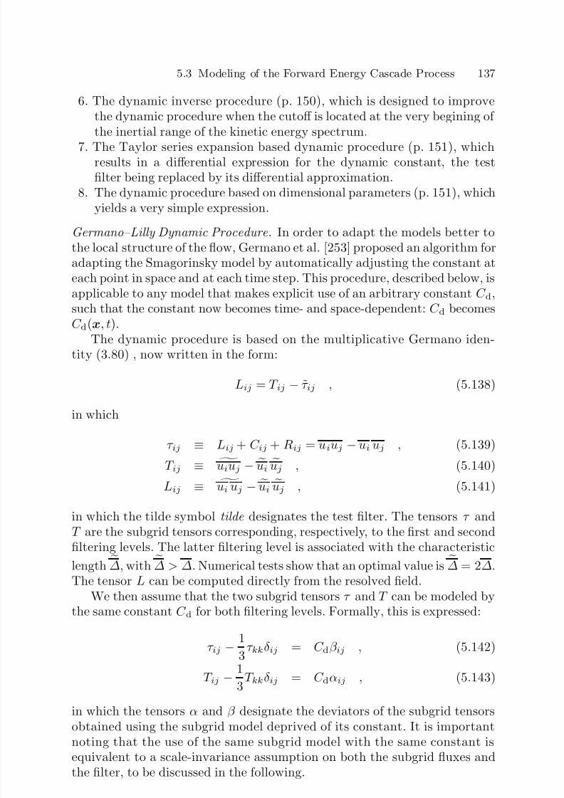
7/21/2019 Large Eddy Simulation for Incompressible Flows
http://slidepdf.com/reader/full/large-eddy-simulation-for-incompressible-flows 159/573
5.3 Modeling of the Forward Energy Cascade Process 137
6. The dynamic inverse procedure (p. 150), which is designed to improvethe dynamic procedure when the cutoff is located at the very begining of the inertial range of the kinetic energy spectrum.
7. The Taylor series expansion based dynamic procedure (p. 151), whichresults in a differential expression for the dynamic constant, the testfilter being replaced by its differential approximation.
8. The dynamic procedure based on dimensional parameters (p. 151), whichyields a very simple expression.
Germano–Lilly Dynamic Procedure. In order to adapt the models better tothe local structure of the flow, Germano et al. [253] proposed an algorithm foradapting the Smagorinsky model by automatically adjusting the constant at
each point in space and at each time step. This procedure, described below, isapplicable to any model that makes explicit use of an arbitrary constant C d,such that the constant now becomes time- and space-dependent: C d becomesC d(x, t).
The dynamic procedure is based on the multiplicative Germano iden-tity (3.80) , now written in the form:
Lij = T ij − τ ij , (5.138)
in which
τ ij ≡ Lij + C ij + Rij = uiuj − ui uj , (5.139)
T ij ≡ uiuj − ui uj , (5.140)
Lij ≡ ui uj − ui uj , (5.141)
in which the tilde symbol tilde designates the test filter. The tensors τ andT are the subgrid tensors corresponding, respectively, to the first and secondfiltering levels. The latter filtering level is associated with the characteristic
length ∆, with ∆ > ∆. Numerical tests show that an optimal value is ∆ = 2∆.The tensor L can be computed directly from the resolved field.
We then assume that the two subgrid tensors τ and T can be modeled bythe same constant C d for both filtering levels. Formally, this is expressed:
τ ij − 1
3τ kkδ ij = C dβ ij , (5.142)
T ij − 1
3T kkδ ij = C dαij , (5.143)
in which the tensors α and β designate the deviators of the subgrid tensorsobtained using the subgrid model deprived of its constant. It is importantnoting that the use of the same subgrid model with the same constant isequivalent to a scale-invariance assumption on both the subgrid fluxes andthe filter, to be discussed in the following.
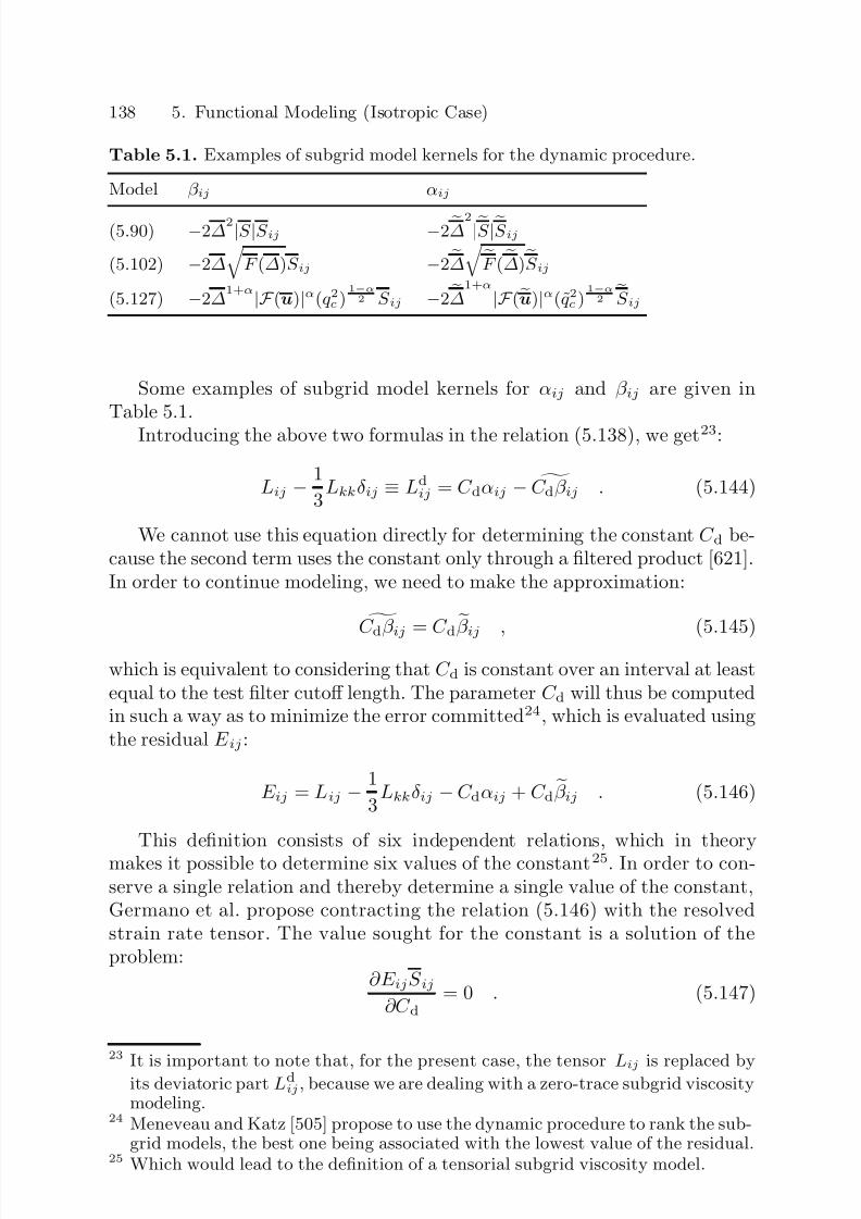
7/21/2019 Large Eddy Simulation for Incompressible Flows
http://slidepdf.com/reader/full/large-eddy-simulation-for-incompressible-flows 160/573
138 5. Functional Modeling (Isotropic Case)
Table 5.1. Examples of subgrid model kernels for the dynamic procedure.
Model β ij αij
(5.90) −2∆2|S |S ij −2∆2|S |S ij
(5.102) −2∆
F (∆)S ij −2∆ F (∆)S ij
(5.127) −2∆1+α|F (u)|α(q 2c )
1−α2 S ij −2∆1+α
|F (u)|α(q 2c )1−α2 S ij
Some examples of subgrid model kernels for αij and β ij are given inTable 5.1.
Introducing the above two formulas in the relation (5.138), we get23:
Lij − 1
3Lkkδ ij ≡ Ld
ij = C dαij − C dβ ij . (5.144)
We cannot use this equation directly for determining the constant C d be-cause the second term uses the constant only through a filtered product [621].In order to continue modeling, we need to make the approximation:
C dβ ij = C dβ ij , (5.145)
which is equivalent to considering that C d is constant over an interval at leastequal to the test filter cutoff length. The parameter C d will thus be computedin such a way as to minimize the error committed24, which is evaluated usingthe residual E ij :
E ij = Lij − 1
3Lkkδ ij − C dαij + C dβ ij . (5.146)
This definition consists of six independent relations, which in theorymakes it possible to determine six values of the constant25. In order to con-serve a single relation and thereby determine a single value of the constant,Germano et al. propose contracting the relation (5.146) with the resolvedstrain rate tensor. The value sought for the constant is a solution of theproblem:
∂E ijS ij∂C d
= 0 . (5.147)
23
It is important to note that, for the present case, the tensor Lij is replaced byits deviatoric part Ldij , because we are dealing with a zero-trace subgrid viscosity
modeling.24 Meneveau and Katz [505] propose to use the dynamic procedure to rank the sub-
grid models, the best one being associated with the lowest value of the residual.25 Which would lead to the definition of a tensorial subgrid viscosity model.
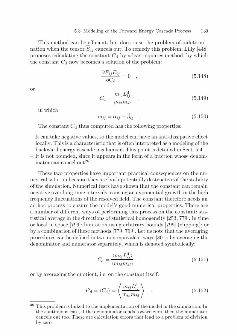
7/21/2019 Large Eddy Simulation for Incompressible Flows
http://slidepdf.com/reader/full/large-eddy-simulation-for-incompressible-flows 161/573
5.3 Modeling of the Forward Energy Cascade Process 139
This method can be efficient, but does raise the problem of indetermi-nation when the tensor S ij cancels out. To remedy this problem, Lilly [448]proposes calculating the constant C d by a least-squares method, by whichthe constant C d now becomes a solution of the problem:
∂E ijE ij∂C d
= 0 , (5.148)
or
C d =mijLd
ij
mklmkl, (5.149)
in which
mij = αij − β ij . (5.150)The constant C d thus computed has the following properties:
– It can take negative values, so the model can have an anti-dissipative effectlocally. This is a characteristic that is often interpreted as a modeling of thebackward energy cascade mechanism. This point is detailed in Sect. 5.4.
– It is not bounded, since it appears in the form of a fraction whose denom-inator can cancel out26.
These two properties have important practical consequences on the nu-merical solution because they are both potentially destructive of the stabilityof the simulation. Numerical tests have shown that the constant can remainnegative over long time intervals, causing an exponential growth in the highfrequency fluctuations of the resolved field. The constant therefore needs anad hoc process to ensure the model’s good numerical properties. There area number of different ways of performing this process on the constant: sta-tistical average in the directions of statistical homogeneity [253, 779], in timeor local in space [799]; limitation using arbitrary bounds [799] (clipping); orby a combination of these methods [779, 799]. Let us note that the averaging
procedures can be defined in two non-equivalent ways [801]: by averaging thedenominator and numerator separately, which is denoted symbolically:
C d =mijLd
ijmklmkl , (5.151)
or by averaging the quotient, i.e. on the constant itself:
C d =
C d
=
mijLdij
mklmkl . (5.152)
26 This problem is linked to the implementation of the model in the simulation. Inthe continuous case, if the denominator tends toward zero, then the numeratorcancels out too. These are calculation errors that lead to a problem of divisionby zero.
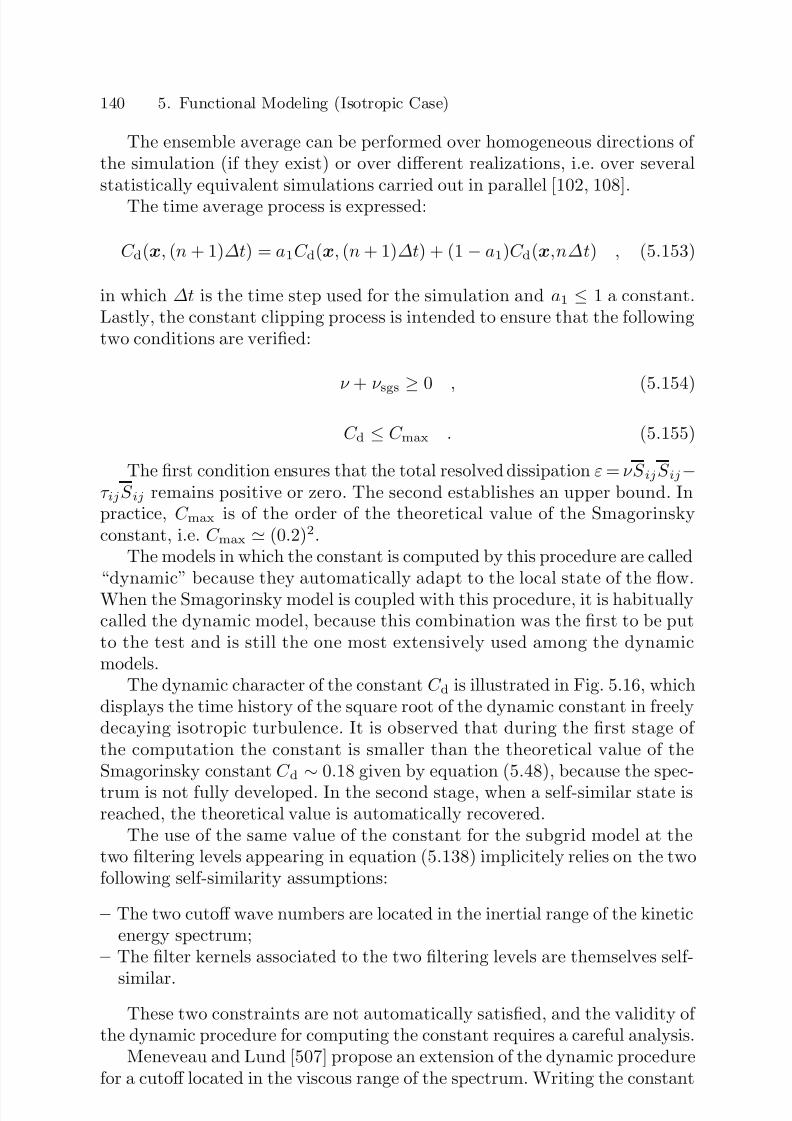
7/21/2019 Large Eddy Simulation for Incompressible Flows
http://slidepdf.com/reader/full/large-eddy-simulation-for-incompressible-flows 162/573
140 5. Functional Modeling (Isotropic Case)
The ensemble average can be performed over homogeneous directions of the simulation (if they exist) or over different realizations, i.e. over severalstatistically equivalent simulations carried out in parallel [102, 108].
The time average process is expressed:
C d(x, (n + 1)∆t) = a1C d(x, (n + 1)∆t) + (1 − a1)C d(x,n∆t) , (5.153)
in which ∆t is the time step used for the simulation and a1 ≤ 1 a constant.Lastly, the constant clipping process is intended to ensure that the followingtwo conditions are verified:
ν + ν sgs ≥
0 , (5.154)
C d ≤ C max . (5.155)
The first condition ensures that the total resolved dissipation ε = νS ijS ij−τ ijS ij remains positive or zero. The second establishes an upper bound. Inpractice, C max is of the order of the theoretical value of the Smagorinskyconstant, i.e. C max (0.2)2.
The models in which the constant is computed by this procedure are called“dynamic” because they automatically adapt to the local state of the flow.When the Smagorinsky model is coupled with this procedure, it is habituallycalled the dynamic model, because this combination was the first to be putto the test and is still the one most extensively used among the dynamicmodels.
The dynamic character of the constant C d is illustrated in Fig. 5.16, whichdisplays the time history of the square root of the dynamic constant in freelydecaying isotropic turbulence. It is observed that during the first stage of the computation the constant is smaller than the theoretical value of theSmagorinsky constant C d
∼0.18 given by equation (5.48), because the spec-
trum is not fully developed. In the second stage, when a self-similar state isreached, the theoretical value is automatically recovered.
The use of the same value of the constant for the subgrid model at thetwo filtering levels appearing in equation (5.138) implicitely relies on the twofollowing self-similarity assumptions:
– The two cutoff wave numbers are located in the inertial range of the kineticenergy spectrum;
– The filter kernels associated to the two filtering levels are themselves self-
similar.
These two constraints are not automatically satisfied, and the validity of the dynamic procedure for computing the constant requires a careful analysis.
Meneveau and Lund [507] propose an extension of the dynamic procedurefor a cutoff located in the viscous range of the spectrum. Writing the constant

7/21/2019 Large Eddy Simulation for Incompressible Flows
http://slidepdf.com/reader/full/large-eddy-simulation-for-incompressible-flows 163/573
5.3 Modeling of the Forward Energy Cascade Process 141
Fig. 5.16. Time history of the square root of the dynamic constant in large-eddysimulation of freely decaying isotropic turbulence (dynamic Smagorinsky model).Courtesy of E. Garnier, ONERA.
of the subgrid-scale model C as an explicit function of the filter characteristiclength, the Germano–Lilly procedure leads to
C (∆) = C (∆) = C d . (5.156)
Let η be the Kolmogorov length scale. It was said in the introductionthat the flow is fully resolved if ∆ = η. Therefore, the dynamic procedure isconsistent if, and only if
lim∆→η
C d = C (η) = 0 . (5.157)
Numerical experiments carried out by the two authors show that theGermano–Lilly procedure is not consistent, because it returns the value of the constant associated to the test filter level
C d = C (
∆) , (5.158)
yieldinglim∆→η
C d = C (rη) = 0, r = ∆/∆ . (5.159)
Numerical tests also showed that taking the limit r → 1 or computing thetwo values C (∆) and C (r∆) using least-square-error minimization without

7/21/2019 Large Eddy Simulation for Incompressible Flows
http://slidepdf.com/reader/full/large-eddy-simulation-for-incompressible-flows 164/573
142 5. Functional Modeling (Isotropic Case)
assuming them to be equal yield inconsistent or ill-behaved solutions. A so-lution is to use prior knowledge to compute the dynamic constant. A robustalgorithm is obtained by rewriting equation (5.146) as follows:
E ij = Ldij − C (∆)
f (∆, r)αij − β ij
, (5.160)
where f (∆, r) = C (r∆)/C (∆) is evaluated by calculations similar to those of Voke (see page 118). A simple analytical fitting is obtained in the case r = 2:
f (∆, 2) ≈ max(100, 10−x), x = 3.23(Re−0.922∆
− Re−0.92∆
) , (5.161)
where the mesh-Reynolds numbers are evaluated as (see equation (5.70)):
Re∆ = ∆
2|S |ν
, Re2∆ = 4∆
2|S |ν
.
Other cases can be considered where the similarity hypothesis betweenthe subgrid stresses at different resolution levels may be violated, leading todifferent values of the constant [601]. Among them:
– The case of a very coarse resolution, with a cutoff located at the verybeginning of the inertial range or in the production range.
– The case of a turbulence undergoing rapid strains, where a transition length∆T ∝ S −3/2ε1/2 appears. Here, S and ε are the strain magnitude and thedissipation rate, respectively. Dimensional arguments show that, roughlyspeaking, scales larger than ∆T are rapidly distorted but have no timeto adjust dynamically, while scales smaller than ∆T can relax faster vianonlinear interactions.
For each of these cases, scale dependence of the model near the criticallength scale is expected, which leads to a possible loss of efficiency of theclassical Germano–Lilly dynamic procedure.
A more general dynamic procedure, which does not rely on the assumptionof scale similarity or location of the cutoff in the dissipation range, was pro-posed by Porte-Agel et al. [601]. This new scale-dependent dynamic procedureis obtained by considering a third filtering level (i.e. a second test-filtering
level) with a characteristic cutoff length scale ∆ > ∆. Filtered variables atthis new level are denoted by a caret.
Writing the Germano identity between level ∆ and level ∆ leads to
Qij −
1
3
Qkkδ ij ≡ uiuj − ui uj = C ( ∆)γ ij
−C (∆) β ij , (5.162)
where γ ij and β ij denote the expression of the subgrid model at levels ∆ and∆, respectively. By taking
nij =
Λ( ∆, ∆)γ ij − β ij
, (5.163)
7/21/2019 Large Eddy Simulation for Incompressible Flows
http://slidepdf.com/reader/full/large-eddy-simulation-for-incompressible-flows 165/573
5.3 Modeling of the Forward Energy Cascade Process 143
with
Λ( ∆, ∆) = C (
∆)
C (∆)
, (5.164)
we obtain the following value for the constant at level ∆:
C (∆) = nijQijnijnij
. (5.165)
By now considering relation (5.149), which expresses the Germano iden-tity between the first two filtering levels, where mij is now written as
mij = Λ(∆, ∆)αij − β ij , (5.166)
and by equating the values of C (∆) obtained using the two test-filteringlevels, we obtain the following relation:
(Lijmij)(nijnij) − (Qijnij)(mijmij) = 0 , (5.167)
which has two unknowns, Λ(
∆, ∆) and Λ(
∆, ∆). In order to obtain a closed
system, some additional assumptions are needed. It is proposed in [601] to
assume a power-law scaling of the dynamic constant, C (x) ∝ x p
, leading to
C (a∆) = C (∆)ar . (5.168)
For this power-law behavior, the function Λ(., .) does not depend on thescales but only on the ratio of the scales, i.e. Λ(x, y) = (x/y)r. Using this sim-plification, (5.167) appears as a fifth-order polynomial in C (∆). The dynamicconstant is taken equal to the largest root.
We now consider the problem of the filter self-similarity. Let G1 and G2
be the filter kernels associated with the first and second filtering level. For
the sake of simplicity, we use the notations ∆ = ∆1 and ∆ = ∆2. We assumethat the filter kernels are rewritten in a form such that:
u(x) = G1 u(x) =
G1
|x − ξ |∆1
u(ξ )dξ , (5.169)
u(x) = G2 u(x) =
G2
|x − ξ |∆2
u(ξ )dξ . (5.170)
We also introduce the test filter Gt, which is defined such that
u = G2 u = Gt u = Gt G1 u . (5.171)
The filters G1 and G2 are self-similar if and only if
G1(y) = 1
rdG2
y
r
, r = ∆2/∆1 . (5.172)
7/21/2019 Large Eddy Simulation for Incompressible Flows
http://slidepdf.com/reader/full/large-eddy-simulation-for-incompressible-flows 166/573
144 5. Functional Modeling (Isotropic Case)
Hence, the two filters must have identical shapes and may only differ bytheir associated characteristic length. The problem is that in practice onlyGt is known, and the self-similarity property might not be a priori verified.Carati and Vanden Eijnden [104] show that the interpretation of the resolvedfield is fully determined by the choice of the test filter Gt, and that the useof the same model for the two levels of filtering is fully justified. This isdemonstrated by re-interpreting previous filters in the following way. Let usconsider an infinite set of self-similar filters F n ≡ F (ln) defined as
F n(x) = 1
rnF
x
ln
, ln = rnl0 , (5.173)
where F
, r > 1 and l0
are the filter kernel, an arbitrary parameter anda reference length, respectively. Let us introduce a second set F ∗n ≡ F ∗(l∗n)defined by
F ∗n ≡ F n F n−1 ... F −∞ . (5.174)
For positive kernel F , we get the following properties:
– The length l∗n obeys the same geometrical law as ln:
l∗n = rl∗n−1, and l∗n = r√ r2 − 1
ln . (5.175)
– F ∗n constitute a set of self-similar filters.
Using these two set of filters, the classical filters involved in the dynamicprocedure can be defined as self-similar filters:
Gt(∆t) = F n(ln) , (5.176)
G1(∆1) = F ∗n−1(l∗n−1) , (5.177)
G2(∆2) = F ∗n(l∗n) . (5.178)
For any test-filter Gt and any value of r, the first filter operator can beconstructed explicitly:
G1 = Gt(∆t/r) Gt(∆t/r2) . . . Gt(∆t/r∞) . (5.179)
This relation shows that for any test filter of the form (5.176), the twofiltering operators can be rewritten as self-similar ones, justifying the use of the same model at all the filtering levels.
Lagrangian Dynamic Procedure. The constant regularization procedures
based on averages in the homogeneous directions have the drawback of notbeing usable in complex configurations, which are totally inhomogeneous.One technique for remedying this problem is to take this average along thefluid particle trajectories. This new procedure [508], called the dynamic La-grangian procedure, has the advantage of being applicable in all configura-tions.

7/21/2019 Large Eddy Simulation for Incompressible Flows
http://slidepdf.com/reader/full/large-eddy-simulation-for-incompressible-flows 167/573
5.3 Modeling of the Forward Energy Cascade Process 145
The trajectory of a fluid particle located at position x at time t is, fortimes t previous to t, denoted as:
z(t) = x − tt
u[z(t), t]dt . (5.180)
The residual (5.146) is written in the following Lagrangian form:
E ij(z, t) = Lij(z, t) − C d(x, t)mij(z, t) . (5.181)
We see that the value of the constant is fixed at point x at time t, whichis equivalent to the same linearization operation as for the Germano–Lilly
procedure. The value of the constant that should be used for computing thesubgrid model at x at time t is determined by minimizing the error alongthe fluid particle trajectories. Here too, we reduce to a well-posed problemby defining a scalar residual E lag, which is defined as the weighted integralalong the trajectories of the residual proposed by Lilly:
E lag =
t−∞
E ij(z(t), t)E ij(z(t), t)W (t − t)dt , (5.182)
in which the weighting function W (t−t) is introduced to control the memoryeffect. The constant is a solution of the problem:
∂E lag
∂C d=
t−∞
2E ij(z(t), t)∂E ij(z(t), t)
∂C dW (t − t)dt = 0 , (5.183)
or:
C d(x, t) = J LM
J MM, (5.184)
in which
J LM(x, t) =
t−∞
Lijmij(z(t), t)W (t − t)dt , (5.185)
J MM(x, t) =
t−∞
mijmij(z(t), t)W (t − t)dt . (5.186)
These expressions are non-local in time, which makes them unusable for
the simulation, because they require that the entire history of the simulationbe kept in memory, which exceeds the storage capacities of today’s super-computers. To remedy this, we choose a fast-decay memory function W :
W (t − t) = 1
T lagexp
− t − t
T lag
, (5.187)
7/21/2019 Large Eddy Simulation for Incompressible Flows
http://slidepdf.com/reader/full/large-eddy-simulation-for-incompressible-flows 168/573
146 5. Functional Modeling (Isotropic Case)
in which T lag is the Lagrangian correlation time. With the memory functionin this form, we can get the following equations:
DJ LM
Dt ≡ ∂ J LM
∂t + ui
∂ J LM
∂xi=
1
T lag(Lijmij − J LM) , (5.188)
DJ MM
Dt ≡ ∂ J MM
∂t + ui
∂ J MM
∂xi=
1
T lag(mijmij − J MM) , (5.189)
the solution of which can be used to compute the subgrid model constant ateach point and at each time step. The correlation time T lag is estimated bytests in isotropic homogeneous turbulence at:
T lag(x, t) = 1.5 ∆ (J MMJ LM)−1/8 , (5.190)
which comes down to considering that the correlation time is reduced inthe high-shear regions where J MM is large, and in those regions where thenon-linear transfers are high, i.e. where J LM is large.
This procedure does not guarantee that the constant will be positive,and must therefore be coupled with a regularization procedure. Meneveau etal. [508] recommend a clipping procedure.
Solving equations (5.188) and (5.189) yields a large amount of additionalnumerical work, resulting in a very expensive subgrid model. To alleviate thisproblem, the solution to these two equations may be approximated using thefollowing Lagrangian tracking technique [596]:
J LM(x,n∆t) = a Lij(x,n∆t)mij(x,n∆t)
+ (1 − a)J LM(x − ∆tu(x,n∆t), (n − 1)∆t) , (5.191)
J MM(x,n∆t) = a mij(x,n∆t)mij(x,n∆t)
+ (1 − a)J MM(x − ∆tu(x,n∆t), (n − 1)∆t) , (5.192)
where
a = ∆t/T lag
1 + ∆t/T lag. (5.193)
This new procedure requires only the storage of the two parameters J LM
and J MM at the previous time step and the use of an interpolation procedure.The authors indicate that a linear interpolation is acceptable.
Constrained Localized Dynamic Procedure. Another generalization of theGermano–Lilly dynamic procedure was proposed for inhomogeneous casesby Ghosal et al. [261]. This new procedure is based on the idea of minimiz-ing an integral problem rather than a local one in space, as is done in theGermano–Lilly procedure, which avoids the need to linearize the constant

7/21/2019 Large Eddy Simulation for Incompressible Flows
http://slidepdf.com/reader/full/large-eddy-simulation-for-incompressible-flows 169/573
5.3 Modeling of the Forward Energy Cascade Process 147
when applying the test filter. We now look for the constant C d that willminimize the function F [C d], with
F [C d] = E ij(x)E ij(x)d3x , (5.194)
in which E ij is defined from relation (5.144) and not by (5.146) as was thecase for the previously explained versions of the dynamic procedure. Theconstant sought is such that the variation of F [C d] is zero:
δ F [C d] = 2
E ij(x)δE ij(x)d3x = 0 , (5.195)
or, by replacing E ij with its value: −αijE ijδC d + E ij β ijδC d
d3x = 0 . (5.196)
Expressing the convolution product associated with the test filter, we get: −αijE ij + β ij
E ij(y)G(x − y)d3y
δC d(x)d3x = 0 , (5.197)
from which we deduce the following Euler-Lagrange equation:
−αijE ij + β ij
E ij(y)G(x − y)d3y = 0 . (5.198)
This equation can be re-written in the form of a Fredholm’s integral equa-tion of the second kind for the constant C d:
f (x) = C d(x)
− K(x, y)C d(y)d3y , (5.199)
where
f (x) = 1
αkl(x)αkl(x)
αij(x)Lij(x) − β ij(x)
Lij(y)G(x − y)d3y
,
(5.200)
K(x, y) = KA(x, y) + KA(y, x) + KS (x, y)
αkl(x)αkl(x) , (5.201)
and
KA(x, y) = αij(x)β ij(y)G(x − y) , (5.202)
KS (x, y) =β ij(x)β ij(y)
G(z − x)G(z − y)d3z . (5.203)

7/21/2019 Large Eddy Simulation for Incompressible Flows
http://slidepdf.com/reader/full/large-eddy-simulation-for-incompressible-flows 170/573
148 5. Functional Modeling (Isotropic Case)
This new formulation raises no problems concerning the linearization of the constant, but does not solve the instability problems stemming from thenegative values it may take. This procedure is called the localized dynamicprocedure.
To remedy the instability problem, the authors propose constraining theconstant to remain positive. The constant C d(x) is then expressed as thesquare of a new real variable ξ (x). Replacing the constant with its decompo-sition as a function of ξ , the Euler-Lagrange equation (5.198) becomes:
−αijE ij + β ij
E ij(y)G(x − y)d3y
ξ (x) = 0 . (5.204)
This equality is true if either of the factors is zero, i.e. if ξ (x) = 0 or if therelation (5.198) is verified, which is denoted symbolically C d(x) = G[C d(x)].In the first case, the constant is also zero. To make sure it remains positive,the constant is computed by an iterative procedure:
C (n+1)d (x) =
G[C (n)d (x)] if G[C
(n)d (x)] ≥ 0
0 otherwise
, (5.205)
in which
G[C d(x)] = f (x) − K(x, y)C d(y)d3y . (5.206)
This completes the description of the constrained localized dynamic pro-cedure. It is applicable to all configurations and ensures that the subgridmodel constant remains positive. This solution is denoted symbolically:
C d(x) =
f (x) +
K(x, y)C d(y)d3y
+
, (5.207)
in which + designates the positive part.Approximate Localized Dynamic Procedure. The localized dynamic proceduredecribed in the preceding paragraph makes it possible to regularize the dy-namic procedure in fully non-homogeneous flows, and removes the mathemat-ical inconsistency of the Germano–Lilly procedure. But it requires to solvean integral equation, and thus induces a significant overhead.
To alleviate this problem, Piomelli and Liu [596] propose an ApproximateLocalized Dynamic Procedure, which is not based on a variational approachbut on a time extrapolation process. Equation (5.144) is recast in the form
Ldij = C dαij − C ∗d β ij , (5.208)
where C ∗d is an estimate of the dynamic constant C d, which is assumed tobe known. Writing the new formulation of the residual E ij , the dynamic
7/21/2019 Large Eddy Simulation for Incompressible Flows
http://slidepdf.com/reader/full/large-eddy-simulation-for-incompressible-flows 171/573
5.3 Modeling of the Forward Energy Cascade Process 149
constant is now evaluated as
C d =
αij(Ldij + C ∗d β ij)
αijαij . (5.209)
The authors propose to evaluate the estimate C ∗d by a time extrapolation:
C ∗d = C (n−1)d + ∆t
∂C d∂t
(n−1)
+ ... , (5.210)
where the superscript (n − 1) is related to the value of the variable at the(n−1)th time step, and ∆t is the value of the time step. In practice, Piomelli
and Liu consider first- and second-order extrapolation schemes. The resultingdynamic procedure is fully local, and does not induce large extra computa-tional effort as the original localized procedure does. Numerical experimentscarried out by these authors demonstrate that it still requires clipping toyield a well-behaved algorithm.
Generalized Dynamic Procedure. It is also possible to derive a dynamic pro-cedure using the generalized Germano identity (3.87) [629]. We assume thatthe operator L appearing in equation (3.88) is linear, and that there existsa linear operator
L such that
L(a N ) = aL(N ) + L(a, N ) , (5.211)
where a is a scalar real function and N an arbitrary second rank tensor. Thecomputation of the dynamic constant C d is now based on the minimizationof the residual E ij
E ij = L(Ldij) − C dL(mij) , (5.212)
where Ldij and mij are defined by equations (5.144) and (5.150). A least-
square minimizations yields:
C d =L(Ld
ij)L(mij)
L(mij)L(mij) . (5.213)
The reduction of the residual obtained using this new relation with respectto the classical one is analyzed by evaluating the difference:
δE ij = E ij − L(E ij) , (5.214)
where E ij is given by relation (5.212) and E ij by (5.146). Inserting the
two dynamic constants C d and C d, defined respectively by relations (5.213)and (5.149), we get:
δE ij = (C d − C d)L(mij) + L(C d, mij) . (5.215)

7/21/2019 Large Eddy Simulation for Incompressible Flows
http://slidepdf.com/reader/full/large-eddy-simulation-for-incompressible-flows 172/573
150 5. Functional Modeling (Isotropic Case)
An obvious example for the linear operator L is the divergence operator.The associated L is the gradient operator.
An alternative consisting in minimizing a different form of the residualhas been proposed by Morinishi and Vasilyev [542, 544] and Mossi [550]:
E ij = L(Ldij) − L(C dmij) (5.216)
= L(Ldij) − C dL(mij) − L(C d, mij) . (5.217)
The use of this new form of the residual generally requires solving a dif-ferential equation, and then yields a more complex procedure than theform (5.212).
These two procedures theoretically more accurate results than the classi-cal one, because they provide reduce the error committed on the subgrid forceterm itself, rather than on the subgrid tensor. They also take into accountfor the numerical error associated to the discrete form of L.
Dynamic Inverse Procedure. We have already seen that the use of the dy-namic procedure may induce some problems if the cutoff is not located inthe inertial range of the spectra, but in the viscous one. A similar problemarises if the cutoff wave number associated to the test filter occurs at the verybeginning of the inertial range, or in the production range of the spectrum.
In order to compensate inaccuracies arising from the use of a large filterlength associated with the test filter, Kuerten et al. [415] developed a newapproach, referred to as the Dynamic Inverse Procedure. It relies on the ideathat if a dynamic procedure is developed involving only length scales compa-rable to the basic filter length, self-similarity properties will be preserved andconsistent modeling may result. Such a procedure is obtained by defining thefirst filtering operator G and the second one F by
G = H −1 L, F = H , (5.218)
where L is the classical filter level and H an explicit test filter, whose inverseH −1 is assumed to be known explicitly. Inserting these definitions into theGermano identity (3.80), we get a direct evaluation of the subgrid tensor τ :
[F G, B](ui, uj) = [L,B](ui, uj) (5.219)
= uiuj − uiuj (5.220)
≡ τ ij (5.221)
= [H,B] (H −1 L)(ui, uj)
+(H)
[H −1 L , B](ui, uj) . (5.222)
This new identity can be recast in a form similar to the original Germanoidentity
Lij = τ ij − H T ij , (5.223)

7/21/2019 Large Eddy Simulation for Incompressible Flows
http://slidepdf.com/reader/full/large-eddy-simulation-for-incompressible-flows 173/573
5.3 Modeling of the Forward Energy Cascade Process 151
with
Lij = H ((H −1 ui)(H −1 uj)) − uiuj ,
T ij = H −1 uiuj − (H −1 ui)(H −1 uj) .
The term Lij is explicitly known in practice, and does not require
any modeling. Using the same notation as in the section dedicated to theGermano–Lilly procedure, we get, for the Smagorinsky model:
τ ij = C dβ ij , β ij = −2∆2|S |S ij , (5.224)
T
ij = C dαij , αij = −2 ∆2
| S | S ij , (5.225)
where ∆ and S are the characteristic length and the strain rate tensor asso-ciated to the H −1 L filtering level, respectively. Building the residual E ijas
E ij = Lij − C d(β ij − H αij) = L
ij − C dmij , (5.226)
the least-square-error minimization procedure yields:
C d =
Lijmij
mijmij . (5.227)
In this new procedure, the two lengths involved are ∆ and ∆. Since the
latter is associated to an inverse filtering operator, we get ∆ ≤ ∆, ensur-ing that the dynamic procedure will not bring in lengths associated to theproduction range of the spectrum. In practice, this procedure is observed tosuffer the same stability problems than the Germano–Lilly procedure, andneeds to be used together with a stabilization procedure (averaging, clipping,etc.).
Taylor Series Expansion Based Dynamic Models. The dynamic procedurespresented above rely on the use of a discrete test filter. Chester et al. [129]proposed a new formulation for the dynamic procedure based on the differen-tial approximation of the test filter. All quantities apprearing at the test filterlevel can therefore be rewritten as sums and products of partial derivatives of the resolved velocity field, leading to a new expression of dynamic constantswhich involves only higher-order derivatives of the velocity field.
Dynamic Procedure with Dimensional Constants. The dynamic procedures
described in the preceding paragraphs are designed to find the best values of non-dimensional constants in subgrid scale models. Wong and Lilly [766], fol-lowed by Carati and his co-workers [103] propose to extend this procedure toevaluate dimensional parameters which appear in some models. They applied

7/21/2019 Large Eddy Simulation for Incompressible Flows
http://slidepdf.com/reader/full/large-eddy-simulation-for-incompressible-flows 174/573
152 5. Functional Modeling (Isotropic Case)
this idea to the so-called Kolmogov formulation for the subgrid viscosity:
ν sgs = C∆
4/3
ε
1/3
= C ε∆
4/3
, (5.228)
where the parameter C ε = Cε1/3 has the dimension of the cubic root of the subgrid dissipation rate ε. Introducing this closure at both grid and testfiltering levels, one obtains (the tilde symbol is related to the test filter level):
τ ij = −2C ε∆4/3
S ij (5.229)
T ij = −2C ε
∆
4/3
S ij (5.230)
leading to the following expression of the residual
E ij = Ldij − C ε
∆4/3S ij + C ε∆
4/3S ij
. (5.231)
This expression can be used to generate integral expressions for C ε. A very
simple local definition is recovered further assuming that C ε∆4/3
is almost
constant over distance of the order of
∆. Using the additional property that
the test filter perfectly commutes with spatial derivatives, relation (5.231)
simplifies as
E ij = Ldij − 2C ε
∆
4/3 − ∆4/3 S ij . (5.232)
The least-square optimization method therefore yields the following for-mula for the dynamic C ε:
C ε = 1
2∆4/3
− ∆4/3Ldij
S ij
S ijS ij
. (5.233)
As the original Germano-Lilly procedure for non-dimensional parameters,this procedure suffers some numerical instability problems and must thereforebe regularized using clipping and/or averaging.
Dynamic Procedures Without the Germano Identity.
Multilevel Procedure by Terracol and Sagaut. This method proposed by Ter-racol and Sagaut [709] relies on the hypothesis that the computed resolved
kinetic energy spectrum obeys a power-law like
E (k) = E 0kα , (5.234)
where α is the scaling parameter. It is worth noting that Barenblatt [41]suggests that both E 0 and α might be Reynolds-number dependent. A more

7/21/2019 Large Eddy Simulation for Incompressible Flows
http://slidepdf.com/reader/full/large-eddy-simulation-for-incompressible-flows 175/573
5.3 Modeling of the Forward Energy Cascade Process 153
accurate expression for the kinetic energy spectrum is
E (k) = K 0ε2/3k−5/3(kΛ)ζ , (5.235)
where K 0 = 1.4 is the Kolmogorov constant, Λ a length scale and ζ anintermittency factor. Under this assumption, the mean subgrid dissipationrate across a cutoff wave number kc, ε(kc), scales like
ε(kc) = ε0kγ c , γ = 3α + 5
2 =
3
2ζ . (5.236)
where ε0 is a kc-independent parameter. It is observed that in the Kolmogorovcase (α = −5/3), one obtains γ = 0, leading to a constant dissipation rate.
Let us now introduce a set of cutoff wave numbers kn
, with k1
> k2
> ...The following recursive law is straithgforwardly derived from (5.236)
ε(kn)
ε(kn+1) = Rγ n,n+1, Rn,n+1 =
knkn+1
, (5.237)
leading to the following two-level evaluation of the parameter γ :
γ = log(ε(kn)/ε(kn+1))
log(Rn,n+1) . (5.238)
Now introducing a generic subgrid model for the nth cutoff levelτ nij = C f ij(un, ∆
n) , (5.239)
where C is the constant of the model to be dynamically computed, un theresolved field at the considered cutoff level and ∆
n ≡ π/kn the current cutoff length, the dissipation rate can also be expressed as
ε(kn) = −τ nijS n
ij = −Cf ij(un, ∆n
)S n
ij , (5.240)
where S n
is the resolved strain rate at level n. Equation (5.237) shows that
the ratio ε(kn)/ε(kn+1) is independent of the model constant C . Using thisproperty, Terracol and Sagaut propose to introduce two test filter levels k2
and k3 (k1 being the grid filter level where the equations must be closed, i.e.
∆1
= ∆ ). The intermittency factor γ is then computed using relation (5.238),and one obtains the following evaluation for the subgrid dissipation rate atthe grid filter level:
ε(k1) = Rγ 1,2ε(k2) , (5.241)
where ε(k2) is evaluated using a reliable approximation of the subgrid ten-
sor to close the sequence (in practice, a scale-similarity model is used inRef. [709]). The corresponding value of C for the model at the grid level isthen deduced from (5.240):
C = Rγ 1,2
ε(k2)
−f ij(u, ∆)S ij. (5.242)
7/21/2019 Large Eddy Simulation for Incompressible Flows
http://slidepdf.com/reader/full/large-eddy-simulation-for-incompressible-flows 176/573
154 5. Functional Modeling (Isotropic Case)
Multiscale Method Based on the Kolmogorov-Meneveau Equation. Anotherprocedure was developed by Shao [669, 153] starting from the Kolmogorov-Meneveau equation for filtered third-order velocity structure function:
−4
5rε = DLLL − 6GLLL , (5.243)
where DLLL is the third-order longitudinal velocity correlation of the fil-tered field, GLLL(r) the longitudinal velocity-stress correlation tensor andε = −τ ijS ij the average subgrid dissipation (see p. 126 for additional de-tails).
Now assuming that the following self-similarity law is valid
GLLL(r) ∝ r p , (5.244)
where p = −1/3 corresponds to the Kolmogorov local isotropy hypotheses,one obtains the following relationship for two space increments r1 and r2:
0.8r1ε + DLLL(r1)
0.8r2ε + DLLL(r2)=
r1
r2
−1/3
. (5.245)
Now introducing the same generic subgrid closure as for the Terracol–Sagaut procedure
τ ij = Cf ij(u, ∆) , (5.246)
and inserting it into (5.245) to evaluate ε = −τ ijS ij , taking r1 = ∆ andr2 > r1, the dynamic value of the constant C is
C =
∆r2
−1/3DLLL(r2) − DLLL(∆)
0.8f ij(u, ∆)S ij ∆ − ∆r2−1/3
r2 . (5.247)
The only fixed parameter in the Shao procedure is the scaling parameter pin (5.244). This parameter can be computed dynamically introducing a thirdspace increment r3, leading to the definition of a dynamic procedure with thesame properties as the one proposed by Terracol and Sagaut. The proposal of Shao can also be extended to subgrid models with several adjustable constantby introducing an additional space increment for each new constant andsolving a linear algebra problem.
Structural Sensors. Selective Models. In order to improve the pre-diction of intermittent phenomena, we introduce a sensor based on struc-tural information. This is done by incorporating a selection function in themodel, based on the local angular fluctuations of the vorticity, developed byDavid [166, 440].
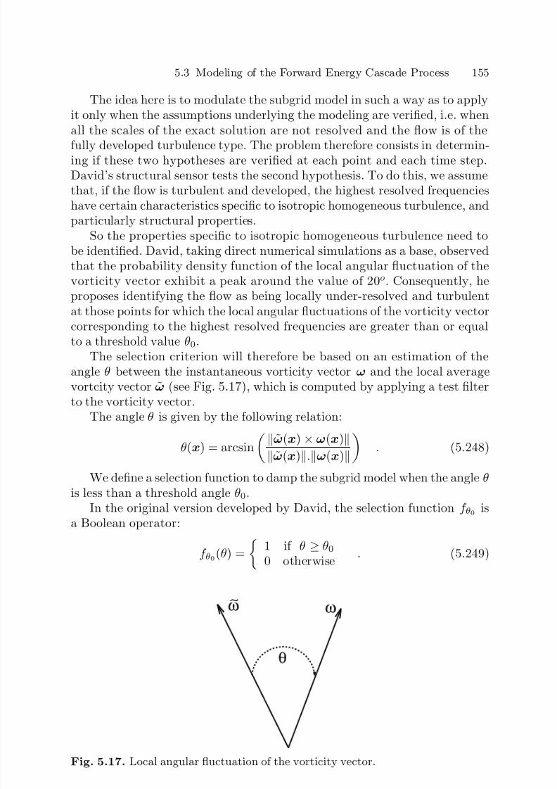
7/21/2019 Large Eddy Simulation for Incompressible Flows
http://slidepdf.com/reader/full/large-eddy-simulation-for-incompressible-flows 177/573
5.3 Modeling of the Forward Energy Cascade Process 155
The idea here is to modulate the subgrid model in such a way as to applyit only when the assumptions underlying the modeling are verified, i.e. whenall the scales of the exact solution are not resolved and the flow is of thefully developed turbulence type. The problem therefore consists in determin-ing if these two hypotheses are verified at each point and each time step.David’s structural sensor tests the second hypothesis. To do this, we assumethat, if the flow is turbulent and developed, the highest resolved frequencieshave certain characteristics specific to isotropic homogeneous turbulence, andparticularly structural properties.
So the properties specific to isotropic homogeneous turbulence need tobe identified. David, taking direct numerical simulations as a base, observedthat the probability density function of the local angular fluctuation of the
vorticity vector exhibit a peak around the value of 20o. Consequently, heproposes identifying the flow as being locally under-resolved and turbulentat those points for which the local angular fluctuations of the vorticity vectorcorresponding to the highest resolved frequencies are greater than or equalto a threshold value θ0.
The selection criterion will therefore be based on an estimation of theangle θ between the instantaneous vorticity vector ω and the local averagevortcity vector ω (see Fig. 5.17), which is computed by applying a test filterto the vorticity vector.
The angle θ is given by the following relation:
θ(x) = arcsin
ω(x) × ω(x)ω(x).ω(x)
. (5.248)
We define a selection function to damp the subgrid model when the angle θis less than a threshold angle θ0.
In the original version developed by David, the selection function f θ0 isa Boolean operator:
f θ0(θ) = 1 if θ ≥
θ00 otherwise . (5.249)
Fig. 5.17. Local angular fluctuation of the vorticity vector.

7/21/2019 Large Eddy Simulation for Incompressible Flows
http://slidepdf.com/reader/full/large-eddy-simulation-for-incompressible-flows 178/573
156 5. Functional Modeling (Isotropic Case)
This function is discontinuous, which may pose problems in the numericalsolution. One variant of it that exhibits no discontinuity for the thresholdvalue is defined as follows [636]:
f θ0(θ) =
1 if θ ≥ θ0
r(θ)n otherwise , (5.250)
in which θ0 is the chosen threshold value and r the function:
r(θ) = tan2(θ/2)
tan2(θ0/2) , (5.251)
where the exponent n is positive. In practice, it is taken to be equal to 2.
Considering the fact that we can express the angle θ as a function of thenorms of the vorticity vector ω, the average vorticity vector ω, and the normω of the fluctuating vorticity vector defined as ω = ω − ω, by the relation:
ω2
= ω2 + ω2 − 2ωω cos θ ,
and the trigonometric relation:
tan2(θ/2) = 1 − cos θ
1 + cos θ ,
the quantity tan2(θ/2) is estimated using the relation:
tan2(θ/2) = 2ωω − ω2 − ω2 + ω
2
2ωω + ω2 + ω2 − ω2 . (5.252)
The selection function is used as a multiplicative factor of the subgridviscosity, leading to the definition of selective models:
ν sgs = ν sgs(x, t)f θ0(θ(x)) , (5.253)
in which ν sgs is calculated by an arbitrary subgrid viscosity model. It shouldbe noted that, in order to keep the same average subgrid viscosity value overthe entire fluid domain, the constant that appears in the subgrid model hasto be multiplied by a factor of 1.65. This factor is evaluated on the basis of isotropic homogeneous turbulence simulations.
Accentuation Technique. Filtered Models.
Accentuation Technique. Since large-eddy simulation is based on a frequency
selection, improving the subgrid models in the physical space requires a betterdiagnostic concerning the spectral distribution of the energy in the calculatedsolution. More precisely, what we want to do here is to determine if the ex-act solution is entirely resolved, in which case the subgrid model should bereduced to zero, or if there exist subgrid scales that have to be taken intoaccount by means of a model. When models expressed in the physical space
7/21/2019 Large Eddy Simulation for Incompressible Flows
http://slidepdf.com/reader/full/large-eddy-simulation-for-incompressible-flows 179/573
5.3 Modeling of the Forward Energy Cascade Process 157
do not use additional variables, they suffer from imprecision due to Gabor-Heisenberg’s principle of uncertainty already mentioned above, because thecontribution of the low frequencies precludes any precise determination of the energy at the cutoff. Let us recall that, if this energy is zero, the exactsolution is completely represented and, if otherwise, then subgrid modes ex-ist. In order to be able to detect the existence of the subgrid modes better,Ducros [204, 205] proposes an accentuation technique which consists in ap-plying the subgrid models to a modified velocity field obtained by applyinga frequency high-pass filter to the resolved velocity field. This filter, denotedHPn, is defined recursively as:
HP1(u)
∆
2
∇2u , (5.254)
HPn(u) = HP(HPn−1(u)) . (5.255)
We note that the application of this filter in the discrete case results ina loss of localness in the physical space, which is in conformity with Gabor-Heisenberg’s principle of uncertainty. We use E HPn(k) to denote the energyspectrum of the field thus obtained. This spectrum is related to the initialspectrum E (k) of the resolved scales by:
E HPn(k) = T HPn(k)E (k) , (5.256)
in which T HPn(k) is a transfer function which Ducros evaluates in the form:
T HPn(k) = bn
k
kc
γn. (5.257)
Here, b and γ are positive constants that depend on the discrete filter usedin the numerical simulation27. The shape of the spectrum obtained by thetransfer function to a Kolmogorov spectrum is graphed in Fig. 5.18 for severalvalues of the parameter n. This type of filter modifies the spectrum of the
initial solution by emphasizing the contribution of the highest frequencies.The resulting field therefore represents mainly the high frequencies of the
initial field and serves to compute the subgrid model. To remain consistent,the subgrid model has to be modified. Such models are called filtered models.The case of the Structure Function model is given as an example. Filteredversions of the Smagorinsky and Mixed Scale models have been developpedby Sagaut, Comte and Ducros [628].
Filtered Second-Order Structure Function Model. We define the second-order
structure function of the filtered field:
DHPn
LL (x, r, t) =
|x|=r
[HPn(u)(x, t) − HPn(u)(x + x, t)]2
d3x , (5.258)
27 For a Laplacian type filter discretized by second-order accurate finite differencescheme iterated three times (n = 3), Ducros finds b3 = 64, 000 and 3γ = 9.16.

7/21/2019 Large Eddy Simulation for Incompressible Flows
http://slidepdf.com/reader/full/large-eddy-simulation-for-incompressible-flows 180/573
158 5. Functional Modeling (Isotropic Case)
Fig. 5.18. Energy spectrum of the accentuation solution for different values of theparameter n (b = γ = 1, kc = 1000).
for which the statistical average over the entire fluid domain, denoted
DHPn
LL (r, t), is related to the kinetic energy spectrum by the relation:
DHPn
LL (r, t) = 4
kc0
E HPn(k)
1−
sin(k∆)
k∆
dk . (5.259)
According to the theorem of averages, there exists a wave number k∗ ∈[0, kc] such that:
E HPn
(k∗
) =
DHPn
LL (r, t)
4(π/kc) π0
(1− sin(ξ )/ξ ) dξ . (5.260)
Using a Kolmogorov spectrum, we can state the equality:
E (kc)
k−5/3c
= E HPn(k∗)
k∗. (5.261)
Considering this last relation, along with (5.256) and (5.257), the subgrid
viscosity models based on the energy at cutoff are expressed:
ν sgs = 2
3
K −3/20
k1/2c
k∗kc
5/3−γn1
bnE HPn(k∗) , (5.262)

7/21/2019 Large Eddy Simulation for Incompressible Flows
http://slidepdf.com/reader/full/large-eddy-simulation-for-incompressible-flows 181/573
5.3 Modeling of the Forward Energy Cascade Process 159
in which:
k∗kc−5/3+γn
= 1π−5/3+γn
π
0
ξ −5/3+γn (1
−sin(ξ )/ξ ) dξ π
0
(1 − sin(ξ )/ξ ) dξ . (5.263)
By localizing these relations in the physical space, we deduce the filteredstructure function model:
ν sgs(x, ∆ , t) = 2
3
K −3/20
π4/3
∆
2
πγn
bn
1/2
D
HPn
LL (x, ∆ , t)1/2
π
0
ξ −5/3+γn (1
−sin(ξ )/ξ ) dξ
1/2
= C (n)∆
DHPn
LL (x, ∆ , t) . (5.264)
The values of the constant C (n) are given in the following Table:In practice, Ducros recommends using n = 3.
Table 5.2. Values of the Structure Function model constant for different iterationsof the high-pass filter.
n 0 1 2 3 4
C (n) 0.0637 0.020 0.0043 0.000841 1.57 · 10−4
Damping Functions for the Near-wall Region. The presence of a solidwall modifies the turbulence dynamics in several ways, which are discussedin Chap. 10. The only fact concerning us here is that the presence of a wallinhibits the growth of the small scales. This phenomenon implies that thecharacteristic mixing length of the subgrid modes ∆f has to be reduced in
the near-surface region, which corresponds to a reduction in the intensityof the subgrid viscosity. To represent the dynamics in the near-wall regioncorrectly, it is important to make sure that the subgrid models verify thegood properties in this region. In the case of a canonical boundary layer (seeChap. 10), the statistical asymptotic behavior of the velocity components andsubgrid tensions can be determined analytically. Let u be the main velocitycomponent in the x direction, v the transverse component in the y direction,and w the velocity component normal to the wall, in the z direction. Usingthe incompressibility constraint, a Taylor series expansion of the velocitycomponent in the region very near the wall yields:
u ∝ z, v ∝ z, w ∝ z2, (5.265)
τ 11 ∝ z2, τ 22 ∝ z2, τ 33 ∝ z4,
τ 13 ∝ z3, τ 12 ∝ z2, τ 23 ∝ z3. (5.266)

7/21/2019 Large Eddy Simulation for Incompressible Flows
http://slidepdf.com/reader/full/large-eddy-simulation-for-incompressible-flows 182/573
160 5. Functional Modeling (Isotropic Case)
Experience shows that it is important to reproduce the behavior of thecomponent τ 13 in order to ensure the quality of the simulation results. It isgenerally assumed that the most important stress in the near-wall region isτ 13, because it is directly linked to the mean turbulence production term, P ,which is evaluated as
P ∝ τ 13dudz
. (5.267)
Thus, it is expected that subgrid-viscosity models will be such that
ν sgsdudz
∝ τ 13 ∝ z3 . (5.268)
We deduce the following law from relations (5.265) and (5.268):
ν sgs ∝ z3 . (5.269)
We verify that the subgrid-viscosity models based on the large scales alonedo not verify this asymptotic behavior. This is understood by looking at thewall value of the subgrid viscosity associated with the mean velocity fieldu. A second-order Taylor series expansion of some zero-equation subgridviscosity models presented in the preceding section yields:
ν sgs|w ∝ ∆|2w ∂ u
∂z
w
(Smagorinsky) ,
ν sgs|w ∝ ∆|w∆z1
∂ u∂z
w
(2nd order Structure Function) ,
ν sgs|w ∝ ∆|3/2w ∆z1
∂ u∂z
1/2
w
∂ 2u∂z 2
1/2
w
(Mixed Scale) ,
(5.270)
where the w subscript denotes values taken at the wall, and ∆z1 is the dis-tance to the wall at which the model is evaluated. Because ∂ u/∂z is notzero at the wall,28, we have the following asymptotic scalings of the modeledsubgrid viscosity at solid walls:
ν sgs|w = O(∆|2w) (Smagorinsky) ,
ν sgs|w = O(∆|w∆z1) (2nd order Structure Function) ,
ν sgs|w = 0 (Mixed Scale) .
(5.271)
In practice, the Mixed Scale model can predict a zero subgrid viscosityat the wall if the computational grid is fine enough to make it possible to
28 Or, equivalently, the skin friction is not zero.

7/21/2019 Large Eddy Simulation for Incompressible Flows
http://slidepdf.com/reader/full/large-eddy-simulation-for-incompressible-flows 183/573
5.3 Modeling of the Forward Energy Cascade Process 161
evaluate correctly the second-order wall–normal velocity derivative, i.e. if atleast three grid points are located within the region where the mean velocityprofile obeys a linear law. Consequently, the first two models must be modifiedin the near-wall region in order to enforce a correct asymptotic behavior of the subgrid terms in that region.
This is done by introducing damping functions. The usual relation:
∆f = C ∆ , (5.272)
is replaced by:∆f = C ∆f w(z) , (5.273)
in which f w(z) is the damping function and z the distance to the wall. FromVan Driest’s results, we define:
f w(z) = 1 − exp(−zuτ /25ν ) , (5.274)
in which the friction velocity uτ is defined in Sect. 10.2.1. Piomelli et al. [600]propose the alternate form:
f w(z) =
1 − exp
−(zuτ /25ν )3
1/2
. (5.275)
From this last form we can get a correct asymptotic behavior of the sub-grid viscosity, i.e. a decrease in z+3
in the near-wall region, contrary to theVan Driest function. Experience shows that we can avoid recourse to thesefunctions by using a dynamic procedure, a filtered model, a selective model, orthe Yoshizawa model. It is worth noting that subgrid viscosity models can bedesigned, which automatically follow the correct behavior in the near-wall re-gion. An example is the WALE model, developed by Nicoud and Ducros [567].
5.3.4 Implicit Diffusion: the ILES Concept
Large-eddy simulation approaches using a numerical viscosity with no explicitmodeling are all based implicitly on the hypothesis:
Hypothesis 5.6 The action of subgrid scales on the resolved scales is equiv-alent to a strictly dissipative action.
This approach is referred to as Implicit Large-Eddy Simulation (ILES). Sim-ulations belonging to this category use dissipation terms introduced eitherin the framework of upwind schemes for the convection or explicit artificial
dissipation term, or by the use of implicit [716] or explicit [210] frequency low-pass filters. The approach most used is doubtless the use of upwind schemesfor the convective term. The diffusive term introduced then varies both in de-gree and order, depending on the scheme used (QUICK [437], Godunov [776],PPM [145], TVD [150], FCT [66], MPDATA [489, 488], among others) and
7/21/2019 Large Eddy Simulation for Incompressible Flows
http://slidepdf.com/reader/full/large-eddy-simulation-for-incompressible-flows 184/573
162 5. Functional Modeling (Isotropic Case)
the dissipation induced can in certain cases be very close29 to that introducedby a physical model [275]. Let us note that most of the schemes introducedissipations of the second and/or fourth order and, in so doing, are very closeto subgrid models. This point is discussed more precisely in Chap. 8. This ap-proach is widely used in cases where the other modeling approaches becomedifficult for one of the two following reasons:
– The dynamic mechanisms escape the physical modeling because they areunknown or too complex to be modeled exactly and explicitly, which is truewhen complex thermodynamic mechanisms, for example, interact stronglywith the hydrodynamic mechanisms (e.g. in cases of combustion [135] orshock/turbulence interaction [435]).
– Explicit modeling offers no a priori guarantee of certain realizability con-straints related to the quantities studied (such as the temperature [125]or molar concentrations of pollutants [474]). This point is illustrated inFig. 5.19, which displays the probability density function of a passive scalarcomputed by Large-Eddy Simulation with different numerical schemes forthe convection term.
In cases belonging to one of these two classes, the error committed byusing an implicit viscosity may in theory have no more harmful consequenceon the quality of the result obtained than that which would be introduced
by using an explicit model based on inadequate physical considerations. Thisapproach is used essentially for dealing with very complex configurations orthose harboring numerical difficulties, because it allows the use of robustnumerical methods. Nonetheless, high-resolution simulations of flows are be-ginning to make their appearance [756, 602, 776, 274].
A large number of stabilized numerical methods have been used for large-eddy simulation, but only a few of them have been designed for this specificpurpose or more simply have been analyzed in that sense. A few generalapproaches for designing stabilized methods which mimic functional subgrid
modeling are discussed below:
1. The MILES (Monotone Integrated Large Eddy Simulation) approachwithin the framework of flux-limiting finite volume methods, as discussedby Grinstein and Fureby (p. 163).
2. The adaptive flux reconstruction technique within the framework of non-limited finite volume methods, proposed by (p. 165).
3. Finite element schemes with embedded subgrid stabilization (p. 166).4. The use of Spectral Vanishing Viscosities (p. 169) which are well suited
for numerical methods with spectral-like accuracy.5. The high-order filtering technique (p. 170), originally developed withinthe finite-difference framework, and wich is equivalent to some approxi-mate deconvolution based structural models.
29 In the sense where these dissipations are localized at the same points and are of the same order of magnitude.
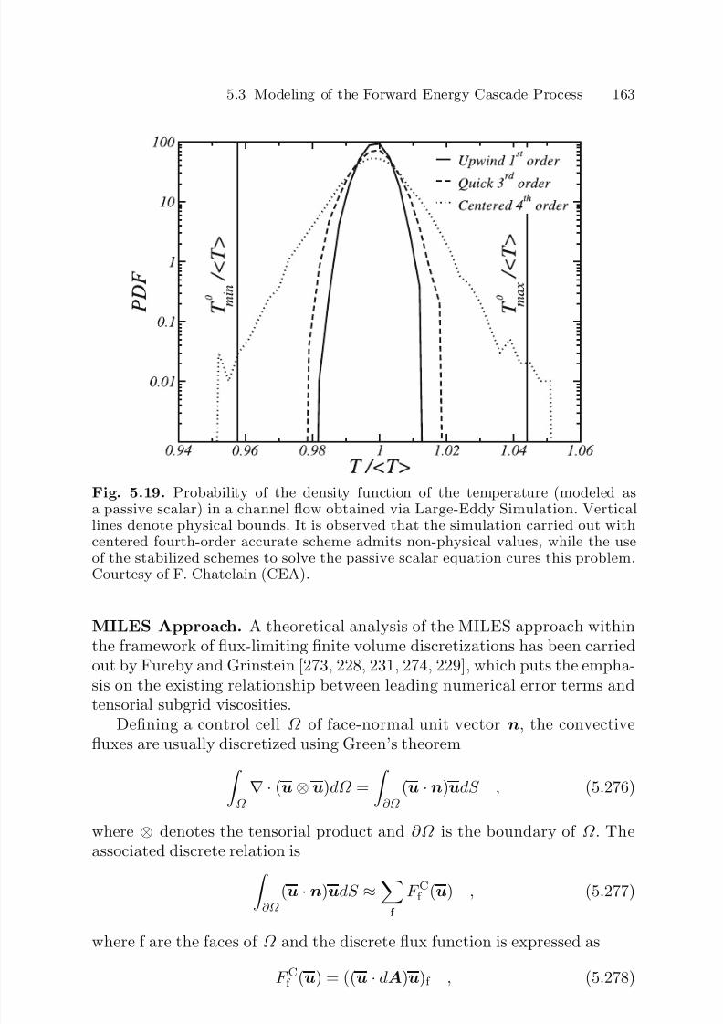
7/21/2019 Large Eddy Simulation for Incompressible Flows
http://slidepdf.com/reader/full/large-eddy-simulation-for-incompressible-flows 185/573
5.3 Modeling of the Forward Energy Cascade Process 163
Fig. 5.19. Probability of the density function of the temperature (modeled asa passive scalar) in a channel flow obtained via Large-Eddy Simulation. Verticallines denote physical bounds. It is observed that the simulation carried out with
centered fourth-order accurate scheme admits non-physical values, while the useof the stabilized schemes to solve the passive scalar equation cures this problem.Courtesy of F. Chatelain (CEA).
MILES Approach. A theoretical analysis of the MILES approach withinthe framework of flux-limiting finite volume discretizations has been carriedout by Fureby and Grinstein [273, 228, 231, 274, 229], which puts the empha-sis on the existing relationship between leading numerical error terms andtensorial subgrid viscosities.
Defining a control cell Ω of face-normal unit vector n, the convectivefluxes are usually discretized using Green’s theorem
Ω
∇ · (u⊗ u)dΩ =
∂Ω
(u ·n)udS , (5.276)
where ⊗ denotes the tensorial product and ∂Ω is the boundary of Ω . Theassociated discrete relation is
∂Ω(u · n)udS ≈f
F
C
f (u) , (5.277)
where f are the faces of Ω and the discrete flux function is expressed as
F Cf (u) = ((u · dA)u)f , (5.278)

7/21/2019 Large Eddy Simulation for Incompressible Flows
http://slidepdf.com/reader/full/large-eddy-simulation-for-incompressible-flows 186/573
164 5. Functional Modeling (Isotropic Case)
where dA is the face-area vector of face f of ∂Ω , and ()f is the integrated valueon face f. For flux-limiting methods, the numerical flux is decomposed as theweighted sum of a high-order flux function F H
f that works well in smooth
regions and a low-order flux function F Lf :
F Cf (u) = F Hf (u) + (1 − Γ (u))
F Hf (u) − F Lf (u)
, (5.279)
where Γ (u) is the flux limiter.30 Fureby and Grinstein analyzed the leadingerror term using the following assumptions: (i) time integration is performedusing a three-point backward scheme, (ii) the high-order flux functions usefirst-order functional reconstruction, and (iii) the low-order flux functionsuse upwind differencing. Retaining the leading dissipative error term, thecontinuous equivalent formulation for the discretized fluxes is
∇ · (u ⊗ u) exact
− ∇ · (u ⊗ r + r ⊗ u + r ⊗ r) dissipative error
, (5.280)
with
r = β (∇u)d, β = 1
2(1 − Γ (u))sgn
u · d
|d|
, (5.281)
where d is the topology vector connecting neighboring control volumes. Com-parison of the error term in (5.280) and the usual subgrid term appearing in
filtered Navier–Stokes equations (3.17) yields the following identification forthe MILES subgrid tensor:
τ MILES = −(u ⊗ r + r ⊗ u + r ⊗ r)
= − β
(u ⊗ d)∇Tu + ∇u(u ⊗ d)T
I
+ β 2(∇u)d ⊗ (∇u)d
II
. (5.282)
Term I appears as a general subgrid-viscosity model with a tensorialdiffusivity β (u ⊗ d), while term II mimics the Leonard tensor, leading tothe definition of an implicit mixed model (see Sect. 7.4).31 A scalar-valuedmeasure of the viscosity is
√ 2/8|u|∆MILES, where the characteristic length
associated with the grid is ∆MILES =
tr[(∇Td)(d ⊗ d)(∇d)].The authors remarked that these error terms are invariant under the
Galilean group of transformations, but are not frame indifferent. Realizabilityand non-negative dissipation of subgrid kinetic energy may be enforced for
some choice of the limiter.30 Many flux limiters can be found in the literature: minmod, superbee, FCT lim-
iter, ... The reader is referred to specialized reference books [307] for a detaileddiscussion of these functions.
31 MILES can also be interpreted as an implicit deconvolution model, using theanalogy discussed in Sect. 7.3.3.

7/21/2019 Large Eddy Simulation for Incompressible Flows
http://slidepdf.com/reader/full/large-eddy-simulation-for-incompressible-flows 187/573
5.3 Modeling of the Forward Energy Cascade Process 165
Adaptive Flux Reconstruction. Adams [2] established a theoretical bridgebetween high-order adaptive flux reconstruction used in certain finite-volumeschemes and the use of a subgrid viscosity. In the simplified case of the fol-lowing one-dimensional conservation law
∂u
∂t +
∂F (u)
∂x = 0 , (5.283)
the finite volume technique leads to the computation of the cell-averagedvariable:
uj =
xj+1/2
xj−1/2
u(ξ )dξ , (5.284)
with ∆x = xj+1/2 − xj−1/2 the cell spacing of the jth cell. High-order finitevolume methods rely on the reconstruction of the unfiltered value uj+1/2 onboth sides of the cell face xj+1/2 on each cell j . This is achieved by defilteringthe variable u and defining a high-order polynomial interpolant.
The defiltering step is similar to the deconvolution approach, whose re-lated results are presented in Sect. 7.2.1 and will not be repeated here. Stick-ing to Adams’ demonstration, a second-order deconvolution is employed:
uj = uj − ∆x2
24∂
2
uj∂x2 . (5.285)
Following the WENO (Weightest Essentially Non-Oscillatory) con-cept [350], a hierarchical family of left-hand-side interpolants of increasingorder is:
P +,(0)(x)j = uj , (5.286)
P +,(1)j (x) = P
+,(0)j (x) + α+
1,1(x
−xj)∆
(1)j , (5.287)
P +,(2)j (x) = P +,(1)
j
+(x−xj)(x−xj+1)
α+1,2∆
(2)j−1 +α+
2,2∆(2)j
, (5.288)
... = ...
where P +,(k)j (x) is the kth-order interpolant, ∆
( p)j the divided difference of
degree p of the variable, and α+m,n some weigthing parameters. Right-hand-
sides are defined in the same way, except that P −,(0)(x)j = uj+1 and weightsare noted α−
m,n. A kth-order interpolation is obtained under the following
constraints: m
α±m,n = 1, α±m,n > 0, n = 1,..,k − 1 . (5.289)
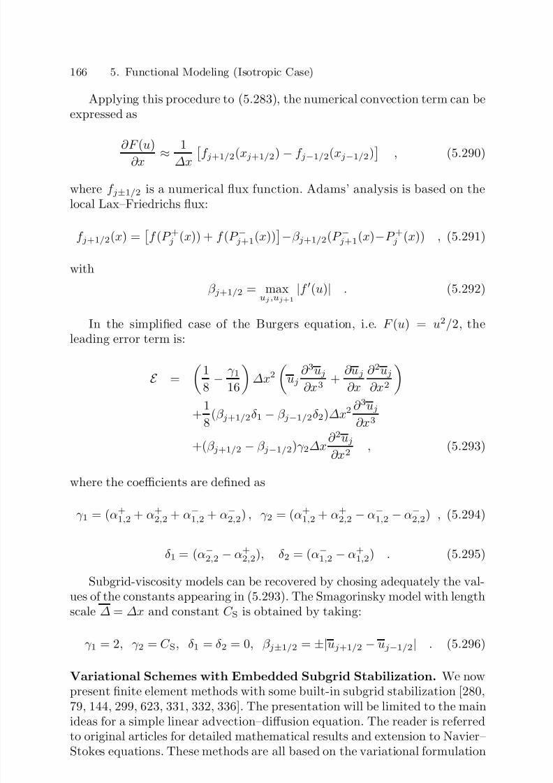
7/21/2019 Large Eddy Simulation for Incompressible Flows
http://slidepdf.com/reader/full/large-eddy-simulation-for-incompressible-flows 188/573
166 5. Functional Modeling (Isotropic Case)
Applying this procedure to (5.283), the numerical convection term can beexpressed as
∂F (u)
∂x ≈ 1
∆x
f j+1/2(xj+1/2) − f j−1/2(xj−1/2)
, (5.290)
where f j±1/2 is a numerical flux function. Adams’ analysis is based on thelocal Lax–Friedrichs flux:
f j+1/2(x) =
f (P +j (x)) + f (P −j+1(x))−β j+1/2(P −j+1(x)−P +j (x)) , (5.291)
withβ j+1/2 = max
uj ,uj+1
|f (u)| . (5.292)
In the simplified case of the Burgers equation, i.e. F (u) = u2/2, theleading error term is:
E =
1
8 − γ 1
16
∆x2
uj
∂ 3uj∂x3
+ ∂uj
∂x
∂ 2uj∂x2
+ 18 (β j+1/2δ 1 − β j−1/2δ 2)∆x2 ∂
3
uj∂x3
+(β j+1/2 − β j−1/2)γ 2∆x∂ 2uj∂x2
, (5.293)
where the coefficients are defined as
γ 1 = (α+1,2 + α+
2,2 + α−1,2 + α−2,2) , γ 2 = (α+1,2 + α+
2,2 − α−1,2 − α−2,2) , (5.294)
δ 1 = (α−2,2 − α+2,2), δ 2 = (α−1,2 − α+
1,2) . (5.295)
Subgrid-viscosity models can be recovered by chosing adequately the val-ues of the constants appearing in (5.293). The Smagorinsky model with lengthscale ∆ = ∆x and constant C S is obtained by taking:
γ 1 = 2, γ 2 = C S, δ 1 = δ 2 = 0, β j±1/2 = ±|uj+1/2 − uj−1/2| . (5.296)
Variational Schemes with Embedded Subgrid Stabilization. We now
present finite element methods with some built-in subgrid stabilization [280,79, 144, 299, 623, 331, 332, 336]. The presentation will be limited to the mainideas for a simple linear advection–diffusion equation. The reader is referredto original articles for detailed mathematical results and extension to Navier–Stokes equations. These methods are all based on the variational formulation
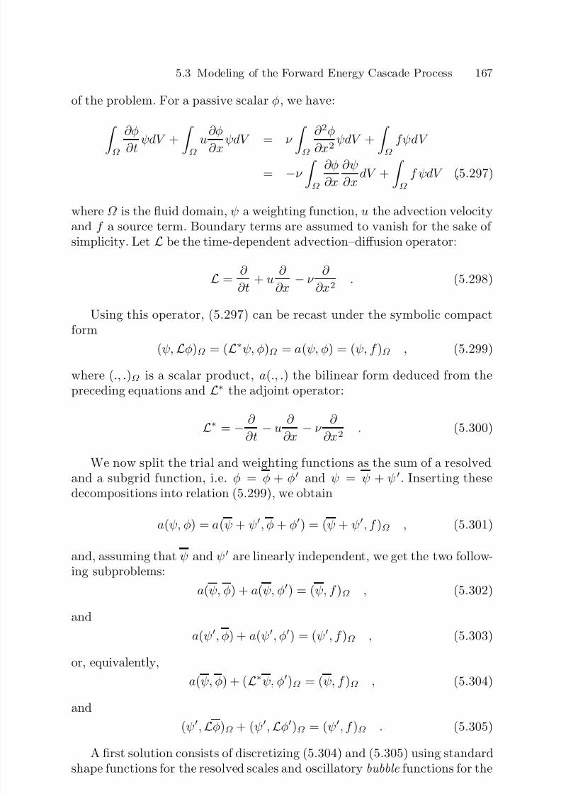
7/21/2019 Large Eddy Simulation for Incompressible Flows
http://slidepdf.com/reader/full/large-eddy-simulation-for-incompressible-flows 189/573
5.3 Modeling of the Forward Energy Cascade Process 167
of the problem. For a passive scalar φ, we have:
Ω
∂φ
∂t ψdV + Ω
u∂φ
∂x ψdV = ν Ω
∂ 2φ
∂x2 ψdV + Ω
fψdV
= −ν
Ω
∂φ
∂x
∂ψ
∂xdV +
Ω
f ψdV ,(5.297)
where Ω is the fluid domain, ψ a weighting function, u the advection velocityand f a source term. Boundary terms are assumed to vanish for the sake of simplicity. Let L be the time-dependent advection–diffusion operator:
L = ∂
∂t + u ∂
∂x − ν ∂
∂x2 . (5.298)
Using this operator, (5.297) can be recast under the symbolic compactform
(ψ, Lφ)Ω = (L∗ψ, φ)Ω = a(ψ, φ) = (ψ, f )Ω , (5.299)
where (., .)Ω is a scalar product, a(., .) the bilinear form deduced from thepreceding equations and L∗ the adjoint operator:
L∗ = − ∂ ∂t
− u ∂ ∂x
− ν ∂ ∂x2
. (5.300)
We now split the trial and weighting functions as the sum of a resolvedand a subgrid function, i.e. φ = φ + φ and ψ = ψ + ψ . Inserting thesedecompositions into relation (5.299), we obtain
a(ψ, φ) = a(ψ + ψ, φ + φ) = (ψ + ψ, f )Ω , (5.301)
and, assuming that ψ and ψ are linearly independent, we get the two follow-ing subproblems:
a(ψ, φ) + a(ψ, φ) = (ψ, f )Ω , (5.302)
and
a(ψ, φ) + a(ψ, φ) = (ψ, f )Ω , (5.303)
or, equivalently,
a(ψ, φ) + (
L∗ψ, φ)Ω = (ψ, f )Ω , (5.304)
and
(ψ, Lφ)Ω + (ψ, Lφ)Ω = (ψ, f )Ω . (5.305)
A first solution consists of discretizing (5.304) and (5.305) using standardshape functions for the resolved scales and oscillatory bubble functions for the

7/21/2019 Large Eddy Simulation for Incompressible Flows
http://slidepdf.com/reader/full/large-eddy-simulation-for-incompressible-flows 190/573
168 5. Functional Modeling (Isotropic Case)
Fig. 5.20. Schematic of the embedded subgrid stabilization approach: linear finiteelement shape functions in one dimension plus typical bubbles
subgrid scales (see Fig. 5.20). The resulting method is a two-scale method,with embedded subgrid stabilization. It is important to note that degrees of freedom associated with bubble functions are eliminated by static condensa-tion, i.e. are expressed as functions of the resolved scales, and do not requirethe solution of additional evolution equations.
Hughes and Stewart [336] proposed regularizing (5.304), which governsthe motion of resolved scales, yielding
a(ψ, φ) + (L∗ψ, M (Lφ− f ))Ω = (ψ, f )Ω , (5.306)
where (Lφ− f ) is the residual of the resolved scales and M an operator orig-inating from an elliptic regularization, which can be evaluated using bubblefunctions.
Usual stabilized methods also rely on the regularization of (5.304) with-out considering the subgrid scale equation. A general form of the stabilizedproblem is
a(ψ, φ) + (ILψ, τ stab(Lφ − f ))Ω = (ψ, f )Ω , (5.307)
where, typically, IL is a differential operator and τ stab is an algebraic operator
which approximates the integral operator (−M ) of (5.306).Classical examples are:
– Standard Galerkin method, which does not introduce any stabilizing term:
IL = 0 . (5.308)
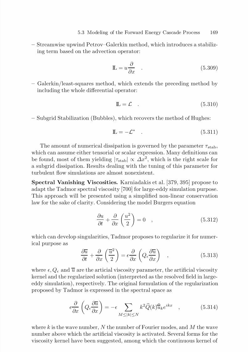
7/21/2019 Large Eddy Simulation for Incompressible Flows
http://slidepdf.com/reader/full/large-eddy-simulation-for-incompressible-flows 191/573
5.3 Modeling of the Forward Energy Cascade Process 169
– Streamwise upwind Petrov–Galerkin method, which introduces a stabiliz-ing term based on the advection operator:
IL = u ∂
∂x . (5.309)
– Galerkin/least-squares method, which extends the preceding method byincluding the whole differential operator:
IL = L . (5.310)
– Subgrid Stabilization (Bubbles), which recovers the method of Hughes:
IL = −L∗ . (5.311)
The amount of numerical dissipation is governed by the parameter τ stab,which can assume either tensorial or scalar expression. Many definitions canbe found, most of them yielding |τ stab| ∝ ∆x2, which is the right scale fora subgrid dissipation. Results dealing with the tuning of this parameter forturbulent flow simulations are almost nonexistent.
Spectral Vanishing Viscosities. Karniadakis et al. [379, 395] propose toadapt the Tadmor spectral viscosity [700] for large-eddy simulation purpose.This approach will be presented using a simplified non-linear conservationlaw for the sake of clarity. Considering the model Burgers equation
∂u
∂t +
∂
∂x
u2
2
= 0 , (5.312)
which can develop singularities, Tadmor proposes to regularize it for numer-ical purpose as
∂u
∂t +
∂
∂x
u2
2
=
∂
∂x
Q
∂u
∂x
, (5.313)
where , Q and u are the articial viscosity parameter, the artificial viscositykernel and the regularized solution (interpreted as the resolved field in large-eddy simulation), respectively. The original formulation of the regularizationproposed by Tadmor is expressed in the spectral space as
∂
∂x Q∂u
∂x = − M ≤|k|≤N
k2 Q(k) uke
ikx
, (5.314)
where k is the wave number, N the number of Fourier modes, and M the wavenumber above which the artificial viscosity is activated. Several forms for theviscosity kernel have been suggested, among which the continuous kernel of

7/21/2019 Large Eddy Simulation for Incompressible Flows
http://slidepdf.com/reader/full/large-eddy-simulation-for-incompressible-flows 192/573
170 5. Functional Modeling (Isotropic Case)
Maday [475] for pseudo-spectral methods based on Legendre polynomials:
Q(k) = exp−(k
−N )2
(k − M )2 , k > M , (5.315)
with M 5√
N and ∼ 1/N . A major difference with spectral functionalmodel in Fourier space is that Tadmor-type regularizations vanish at lowwave numbers, while functional subgrid viscosities don’t. The extension of the method to multidimensional curvilinear grids has been extensivly studiedby Pasquetti and Xu [773, 582, 581].
Karniadakis et al. [395] further modify this model by defining a dynamic
version of the artificial viscosity in which the parameter is tuned regardingthe local state of the flow. To this end, the regularization term is redefinedas
c(x, t)Q∂ 2Qu
∂x2 , (5.316)
where the self-adaptive amplitude parameter c(x, t) can be computed consid-ering either the gradient of the solution
c(x, t) =
κ
N |∇u
|∇u∞ , (5.317)
where κ is an adjustable arbitrary parameter, or the strain tensor
c(x, t) = |S |S ∞
. (5.318)
To prevent a too high dissipation near solid walls, Kirby and Karniadakismultiply Q by a damping function
g(y+) = 2
π tan−1
2ky+
π
1 − exp
−y+
C
2
, (5.319)
where y is he distance to the wall, the superscript + refers to quantitiesexpressed in wall units and C is a parameter.
High-Order Filtered Methods. Visbal and Rizetta define [734] anotherprocedure to perform large-eddy simulation based on numerical stabilization
without explicit physical subgrid model. Their procedure is based on theapplication, at the end of each time, of an high-order low-pass filter to thesolution. This stabilizing procedure and the associated corresponding methodoriginating in the works by Visbal and Gaitonde is discussed in referencesgiven therein. In practice, they use a symmetric compact finite differencefilter with the followng properties:
7/21/2019 Large Eddy Simulation for Incompressible Flows
http://slidepdf.com/reader/full/large-eddy-simulation-for-incompressible-flows 193/573
5.4 Modeling the Backward Energy Cascade Process 171
1. it is non-dispersive, i.e. it is strictly dissipative,2. it does not amplify any waves,3. it preserves constant functions,4. it completely eliminates the odd-even mode.
A tenth-order compact filter is observed to yield satisfactory results insimple cases (decaying isotropic turbulence). It is important to notice thatthis procedure is formally equivalent to the filtering-form of the full decon-volution procedure proposed by Mathew et al. [499] (see p. 220 for details).Therefore, this implicit procedure can be completely rewritten within thestructural modeling framework. Other authors [63] develop similar strate-gies, based on the use of very-high order accurate finite difference schemes.
5.4 Modeling the Backward Energy Cascade Process
5.4.1 Preliminary Remarks
The above models reflect only the forward cascade process, i.e. the dominantaverage effect of the subgrid scales. The second energy transfer mechanism,the backward energy cascade, is much less often taken into account in sim-
ulations. We may mention two reasons for this. Firstly, the intensity of thisreturn is very weak compared with that of the forward cascade toward thesmall scales (at least on the average in the isotropic homogeneous case) andits role in the flow dynamics is still very poorly understood. Secondly, mod-eling it requires the addition of an energy source term to the equations beingcomputed, which is potentially a generator of numerical problems.
Two methods are used for modeling the backward energy cascade:
– Adding a stochastic forcing term constructed from random variables andthe information contained in the resolved field. This approach makes itpossible to include a random character of the subgrid scales, and each sim-ulation can be considered a particular realization. The space-time correla-tions characteristic of the scales originating the backward cascade cannotbe represented by this approach, though, which limits its physical repre-sentativeness.
– Modifying the viscosity associated with the forward cascade mechanism de-fined in the previous section, so as to take the energy injected at the largescales into account. The backward cascade is then represented by a nega-tive viscosity, which is added to that of the cascade model. This approach
is statistical and deterministic, and also subject to caution because it isnot based on a physical description of the backward cascade phenomenonand, in particular, possesses no spectral distribution in k4 predicted by theanalytical theories like EDQNM (see also footnote p. 104). Its advantageresides mainly in the fact that it allows a reduction of the total dissipation
7/21/2019 Large Eddy Simulation for Incompressible Flows
http://slidepdf.com/reader/full/large-eddy-simulation-for-incompressible-flows 194/573
172 5. Functional Modeling (Isotropic Case)
of the simulation, which is generally too high. Certain dynamic proceduresfor automatically computing the constants can generate negative values of them, inducing an energy injection in the resolved field. This property issometimes interpreted as the capacity of the dynamic procedure to reflectthe backward cascade process. This approach can therefore be classed inthe category of statistical deterministic backward cascade models.
Representing the backward cascade by way of a negative viscosity is con-troversial because the theoretical analyses, such as by the EDQNM model,distinguish very clearly between the cascade and backward cascade terms,both in their intensity and in their mathematical form [443, 442]. This rep-resentation is therefore to be linked to other statistical deterministic descrip-
tions of the backward cascade, which take into account only an average reduc-tion of the effective viscosity, such as the Chollet–Lesieur effective viscosityspectral model.
The main backward cascade models belonging to these two categories aredescribed in the following.
5.4.2 Deterministic Statistical Models
This section describes the deterministic models for the backward cascade.
These models, which are based on a modification of the subgrid viscosityassociated with the forward cascade process, are:
1. The spectral model based on the theories of turbulence proposed by Chas-nov (p. 172). A negative subgrid viscosity is computed directly from theEDQNM theory. No hypothesis is adopted concerning the spectrum shapeof the resolved scales, so that the spectral disequilibrium mechanisms canbe taken into account at the level of these scales, but the spectrum shapeof the subgrid scales is set arbitrarily. Also, the filter is assumed to be of the sharp cutoff type.
2. The dynamic model with an equation for the subgrid kinetic energy(p. 173), to make sure this energy remains positive. This ensures thatthe backward cascade process is represented physically, in the sense thata limited quantity of energy can be restored to the resolved scales by thesubgrid modes. However, this approach does not allow a correct repre-sentation of the spectral distribution of the backward cascade. Only thequantity of restored energy is controlled.
Chasnov’s Spectral Model. Chasnov [120] adds a model for the back-ward cascade, also based on an EDQNM analysis, to the forward cascademodel already described (see Sect. 5.3.1). The backward cascade process isrepresented deterministically by a negative effective viscosity term ν −e (k|kc),which is of the form:
ν −e (k|kc, t) = −F −(k|kc, t)
2k2E (k, t) . (5.320)

7/21/2019 Large Eddy Simulation for Incompressible Flows
http://slidepdf.com/reader/full/large-eddy-simulation-for-incompressible-flows 195/573
5.4 Modeling the Backward Energy Cascade Process 173
The stochastic forcing term is computed as:
F −
(k|kc, t) = ∞
kc dp p
p−k dqΘkpqk3
pq (1−2x2
z2
−xyz)E (q, t)E ( p, t), (5.321)
in which x, y , and z are geometric factors associated with the triad (k, p, q),and Θkpq is a relaxation time described in Appendix B. As is done whencomputing the draining term (see Chasnov’s effective viscosity model inSect. 5.3.1), we assume that the spectrum takes the Kolmogorov form be-yond the cutoff kc. To simplify the computations, formula (5.321) is not usedfor wave numbers kc ≤ p ≤ 3kc. For the other wave numbers, we use theasymptotic form
F −(k|kc, t) = 1415
k4 ∞kc
dpΘkpp(t) E 2( p, t) p2
. (5.322)
This expression complete Chasnov’s spectral subgrid model which, thoughquite close to the Kraichnan type effective viscosity models, makes it possibleto take into account the backward cascade effects that are dominant for verysmall wave numbers.
Localized Dynamic Model with Energy Equation. The Germano–Lillydynamic procedure and the localized dynamic procedure lead to the defini-
tion of subgrid models that raise numerical stability problems because themodel constant can take negative values over long time intervals, leading toexponential growth of the disturbances.
This excessive duration of the dynamic constant in the negative state cor-responds to too large a return of kinetic energy toward the large scales [101].This phenomenon can be interpreted as a violation of the spectrum realiz-ability constraint: when the backward cascade is over-estimated, a negativekinetic energy is implicitly defined in the subgrid scales. A simple idea forlimiting the backward cascade consists in guaranteeing spectrum realizabil-
ity32. The subgrid scales cannot then restore more energy than they contain.To verify this constraint, local information is needed on the subgrid kineticenergy, which naturally means defining this as an additional variable in thesimulation.
A localized dynamic model including an energy equation is proposed byGhosal et al. [261]. Similar models have been proposed independently byRonchi et al. [621, 511], Wong [765] and Kim and Menon [391, 392, 583].The subgrid model used is based on the kinetic energy of the subgrid modes.Using the same notation as in Sect. (5.3.3), we get:
αij = −2∆ Q2sgsS ij , (5.323)
β ij = −2∆
q 2sgsS ij , (5.324)
32 The spectrum E (k) is said to be realizable if E (k) ≥ 0, ∀k.
7/21/2019 Large Eddy Simulation for Incompressible Flows
http://slidepdf.com/reader/full/large-eddy-simulation-for-incompressible-flows 196/573
174 5. Functional Modeling (Isotropic Case)
in which the energies Q2sgs and q 2sgs are defined as:
Q2sgs =
1
2 uiui − uiui =
1
2 T ii , (5.325)
q 2sgs = 1
2 (uiui − uiui) =
1
2τ ii . (5.326)
Germano’s identity (5.138) is written:
Q2sgs = q 2sgs +
1
2Lii . (5.327)
The model is completed by calculating q 2sgs by means of an additionalevolution equation. We use the equation already used by Schumann, Horiuti,and Yoshizawa, among others (see Sect. 5.3.1):
∂q 2sgs
∂t +
∂ujq 2sgs
∂xj= −τ ijS ij − C 1
(q 2sgs)3/2
∆
+C 2∂
∂xj
∆
q 2sgs
∂q 2sgs
∂xj
+ ν
∂ 2q 2sgs
∂xj∂xj, (5.328)
in which the constants C 1 and C 2 are computed by a constrained localizeddynamic procedure described above. The dynamic constant C d is computedby a localized dynamic procedure.
This model ensures that the kinetic energy q 2sgs will remain positive, i.e.that the subgrid scale spectrum will be realizable. This property ensures thatthe dynamic constant cannot remain negative too long and thereby destabilizethe simulation. However, finer analysis shows that the realizability conditionsconcerning the subgrid tensor τ (see Sect. 3.3.5) are verified only on thecondition:
− q 2sgs
3∆|sγ | ≤ C d ≤ q 2sgs
3∆sα, (5.329)
where sα and sγ are, respectively, the largest and smallest eigenvalues of the strain rate tensor S . The model proposed therefore does not ensure therealizability of the subgrid tensor.
The two constants C 1 and C 2 are computed using an extension of theconstrained localized dynamic procedure. To do this, we express the kineticenergy Q2
sgs evolution equation as:
∂Q2sgs
∂t +
∂ ujQ2sgs
∂xj= −T ij
S ij − C 1(Q2
sgs)3/2
∆+ C 2
∂
∂xj
Q2
sgs
∂Q2sgs
∂xj
+ ν
∂ 2Q2sgs
∂xj∂xj. (5.330)
7/21/2019 Large Eddy Simulation for Incompressible Flows
http://slidepdf.com/reader/full/large-eddy-simulation-for-incompressible-flows 197/573
5.4 Modeling the Backward Energy Cascade Process 175
One variant of the Germano’s relation relates the subgrid kinetic energyflux f j to its analog at the level of the test filter F j :
F j − f j = Z j ≡ uj ( p + q 2sgs + uiui/2) − uj( p + q 2sgs + uiui/2) , (5.331)
in which p is the resolved pressure.To determine the constant C 2, we substitute in this relation the modeled
fluxes:
f j = C 2∆
q 2sgs
∂q 2sgs
∂xj, (5.332)
F j = C 2∆ Q2
sgs
∂Q2sgs
∂xj, (5.333)
which leads to:
Z j = X jC 2 − Y jC 2 , (5.334)
in which
X j = ∆ Q2sgs
∂Q2sgs
∂xj
, (5.335)
Y j = ∆
q 2sgs
∂q 2sgs
∂xj. (5.336)
Using the same method as was explained for the localized dynamic pro-cedure, the constant C 2 is evaluated by minimizing the quantity:
Z j
−X jC 2 + Y jC 2Z j
−X jC 2 + Y jC 2 . (5.337)
By analogy with the preceding developments, the solution is obtained inthe form:
C 2(x) =
f C 2(x) +
KC 2(x, y)C 2(y)d3y
+
, (5.338)
in which:
f C 2(x) = 1
X j(x)X j(x) X j(x)Z j(x) − Y j(x) Z j(y)G(x − y)d3
y ,
(5.339)
KC 2(x, y) = KC 2A (x, y) + KC 2A (y, x) − KC 2S (x, y)
X j(x)X j(x) , (5.340)

7/21/2019 Large Eddy Simulation for Incompressible Flows
http://slidepdf.com/reader/full/large-eddy-simulation-for-incompressible-flows 198/573
176 5. Functional Modeling (Isotropic Case)
in which
KC 2
A (x, y) = X j(x)Y j(y)G(x
−y) , (5.341)
KC 2S (x, y) = Y j(x)Y j(y)
G(z − x)G(z − y)d3z . (5.342)
This completes the computation of constant C 2. To determine the con-stant C 1, we substitute (5.327) in (5.330) and get:
∂
q 2sgs
∂t
+∂
uj
q 2sgs
∂xj
=
−E
∂F j
∂xj
+ ν ∂ 2
q 2sgs
∂xj∂xj
, (5.343)
in which E is defined as:
E = T ijS ij +
C 1(Q2sgs)
3/2
∆ − ν 1
2
∂ 2Lii∂xj∂xj
+ 1
2
∂Lii
∂t +
∂ ujLii∂xj
. (5.344)
Applying the test filter to relation (5.328), we get:
∂ q 2sgs
∂t +
∂ ujq 2sgs
∂xj= − τ ijS ij −
C 1(q 2sgs)3/2
∆
+
∂ f j∂xj
+ ν ∂ 2q 2sgs
∂xj∂xj. (5.345)
By eliminating the term ∂ q 2sgs/∂t between relations (5.343) and (5.345),
then replacing the quantity F j− f j by its expression (5.331) and the quantityT ij by its value as provided by the Germano identity, we get:
χ = φC 1
− ψC 1 , (5.346)
in which
χ = τ ijS ij − τ ijS ij − Lij
S ij + ∂ρj∂xj
− 1
2DtLii +
1
2ν
∂ 2Lii∂xj∂xj
, (5.347)
φ = (Q2sgs)
3/2/∆ , (5.348)
ψ = (q 2sgs)
3/2
/∆ , (5.349)
and
ρj = uj ( p + uiui/2) − uj( p + uiui/2) . (5.350)

7/21/2019 Large Eddy Simulation for Incompressible Flows
http://slidepdf.com/reader/full/large-eddy-simulation-for-incompressible-flows 199/573
5.4 Modeling the Backward Energy Cascade Process 177
The symbol Dt designates the material derivative ∂/∂t +
uj∂/∂xj. The
constant C 1 is computed by minimizing the quantity
χ − φC 1 + ψC 1
χ − φC 1 + ψC 1
, (5.351)
by a constrained localized dynamic procedure, which is written:
C 1(x) =
f C 1(x) +
KC 1(x, y)C 1(y)d3y
+
, (5.352)
in which
f C 1(x) = 1
φ(x)φ(x)
φ(x)χ(x) − ψ(x)
χ(y)G(x − y)d3y
, (5.353)
KC 1(x, y) = KC 1A (x, y) + KC 1A (y, x) − KC 1S (x, y)
φ(x)φ(x) , (5.354)
in which
KC 1
A (x, y) = φ(x)ψ(y)G(x
−y) , (5.355)
KC 1S (x, y) = ψ(x)ψ(y)
G(z − x)G(z − y)d3z , (5.356)
which completes the computation of the constant C 1.The version by Menon et al. [391, 392, 583], also extensively used by
Davidson and his coworkers [576, 577] is much simpler as far as the practicalimplementation is addressed. This simplified formulation is defined as follows:
C 1 = ∆εtest
(Q2sgs)3/2
, (5.357)
and
C 2 = C d = 1
2
LdijS ijS ijS ij
, (5.358)
where Q2sgs is computed using relation (5.327) and the dissipation at the test
filter level is evaluated using a scale-similarity hypothesis, yielding
εtest = (ν + ν sgs)
∂ui∂xj
∂ui∂xj
−
∂ ui∂xj
∂ ui∂xj
. (5.359)
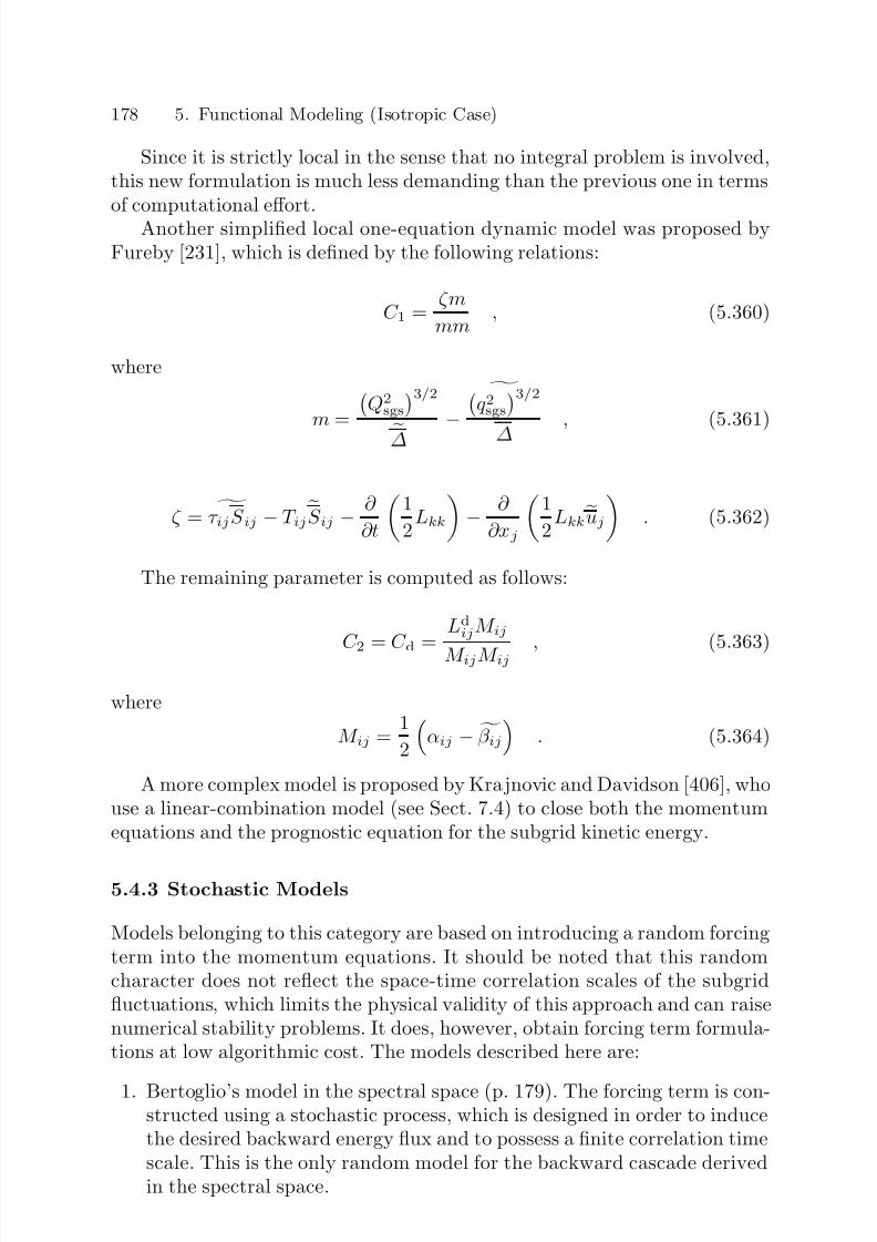
7/21/2019 Large Eddy Simulation for Incompressible Flows
http://slidepdf.com/reader/full/large-eddy-simulation-for-incompressible-flows 200/573
178 5. Functional Modeling (Isotropic Case)
Since it is strictly local in the sense that no integral problem is involved,this new formulation is much less demanding than the previous one in termsof computational effort.
Another simplified local one-equation dynamic model was proposed byFureby [231], which is defined by the following relations:
C 1 = ζm
mm , (5.360)
where
m = Q2
sgs3/2
∆ − q 2sgs
3/2
∆
, (5.361)
ζ = τ ijS ij − T ijS ij − ∂
∂t
1
2Lkk
− ∂
∂xj
1
2Lkkuj . (5.362)
The remaining parameter is computed as follows:
C 2
= C d
=LdijM ij
M ijM ij, (5.363)
where
M ij = 1
2
αij − β ij
. (5.364)
A more complex model is proposed by Krajnovic and Davidson [406], whouse a linear-combination model (see Sect. 7.4) to close both the momentumequations and the prognostic equation for the subgrid kinetic energy.
5.4.3 Stochastic Models
Models belonging to this category are based on introducing a random forcingterm into the momentum equations. It should be noted that this randomcharacter does not reflect the space-time correlation scales of the subgridfluctuations, which limits the physical validity of this approach and can raisenumerical stability problems. It does, however, obtain forcing term formula-tions at low algorithmic cost. The models described here are:
1. Bertoglio’s model in the spectral space (p. 179). The forcing term is con-structed using a stochastic process, which is designed in order to inducethe desired backward energy flux and to possess a finite correlation timescale. This is the only random model for the backward cascade derivedin the spectral space.
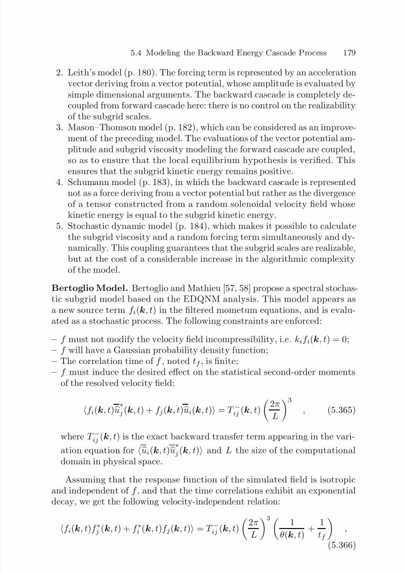
7/21/2019 Large Eddy Simulation for Incompressible Flows
http://slidepdf.com/reader/full/large-eddy-simulation-for-incompressible-flows 201/573
5.4 Modeling the Backward Energy Cascade Process 179
2. Leith’s model (p. 180). The forcing term is represented by an accelerationvector deriving from a vector potential, whose amplitude is evaluated bysimple dimensional arguments. The backward cascade is completely de-coupled from forward cascade here: there is no control on the realizabilityof the subgrid scales.
3. Mason–Thomson model (p. 182), which can be considered as an improve-ment of the preceding model. The evaluations of the vector potential am-plitude and subgrid viscosity modeling the forward cascade are coupled,so as to ensure that the local equilibrium hypothesis is verified. Thisensures that the subgrid kinetic energy remains positive.
4. Schumann model (p. 183), in which the backward cascade is representednot as a force deriving from a vector potential but rather as the divergence
of a tensor constructed from a random solenoidal velocity field whosekinetic energy is equal to the subgrid kinetic energy.
5. Stochastic dynamic model (p. 184), which makes it possible to calculatethe subgrid viscosity and a random forcing term simultaneously and dy-namically. This coupling guarantees that the subgrid scales are realizable,but at the cost of a considerable increase in the algorithmic complexityof the model.
Bertoglio Model. Bertoglio and Mathieu [57, 58] propose a spectral stochas-
tic subgrid model based on the EDQNM analysis. This model appears asa new source term f i(k, t) in the filtered mometum equations, and is evalu-ated as a stochastic process. The following constraints are enforced:
– f must not modify the velocity field incompressibility, i.e. kif i(k, t) = 0;– f will have a Gaussian probability density function;– The correlation time of f , noted tf , is finite;– f must induce the desired effect on the statistical second-order moments
of the resolved velocity field:
f i(k, t) u∗j (k, t) + f j(k, t) ui(k, t) = T −ij (k, t)2πL3
, (5.365)
where T −ij (k, t) is the exact backward transfer term appearing in the vari-
ation equation for ui(k, t) u∗j (k, t) and L the size of the computationaldomain in physical space.
Assuming that the response function of the simulated field is isotropicand independent of f , and that the time correlations exhibit an exponential
decay, we get the following velocity-independent relation:
f i(k, t)f ∗j (k, t) + f ∗i (k, t)f j(k, t) = T −ij (k, t)
2π
L
3 1
θ(k, t) +
1
tf
,
(5.366)

7/21/2019 Large Eddy Simulation for Incompressible Flows
http://slidepdf.com/reader/full/large-eddy-simulation-for-incompressible-flows 202/573
180 5. Functional Modeling (Isotropic Case)
where θ(k, t) is a relaxation time evaluated from the resolved scales. We nowhave to compute the stochastic variable f i. The authors propose the followingalgorithm, which is based on three random variables a, b and c:
f (n+1)1 =
1 − ∆t
tf
f
(n)1 +
h
(n)11 β
(n+1)11
∆t
tf exp(ı2πa(n+1))
+
h
(n)22 β
(n+1)12
∆t
tf exp(ı2πc(n+1)) , (5.367)
f (n+1)2 =
1 − ∆t
tf f
(n)2 +
h
(n)22 β
(n+1)22
∆t
tf exp(ı2πb(n+1))
+
h
(n)11 β
(n+1)21
∆t
tf exp(ı2πc(n+1)) , (5.368)
where the superscript (n) denotes the value at the nth time step, ∆t is thevalue of the time step, and hij(k, t) = f i(k, t)f ∗j (k, t). Moreover, we get thecomplementary set of equations, which close the system:
(β (n+1)11 )2 =
1
h(n)11 (h
(n+1)11
−h
(n)11 )
tf
∆t −h
(n)22 (β
(n+1)12 )2
+2 − ∆t
tf , (5.369)
(β (n+1)22 )2 =
1
h(n)22
(h
(n+1)22 − h
(n)22 )
tf ∆t
− h(n)11 (β
(n+1)21 )2
+2 − ∆t
tf , (5.370)
β
(n+1)
12 β
(n+1)
12 =
1 h(n)11 h
(n)11(h
(n+1)
12 − h
(n)
12 )
tf
∆t
+h(n)12
2 − ∆t
tf
, (5.371)
(β (n+1)21 )2 = (β
(n+1)12 )2 , (5.372)
which completes the description of the model. The resulting random forcesatisfies all the cited constraints, but it requires the foreknowledge of the hijtensor. This tensor is evaluated using the EDQNM theory, which requires
the spectrum of the subgrid scales to be known. To alleviate this problem,arbitrary form of the spectrum can be employed.
Leith Model. A stochastic backward cascade model expressed in the phys-ical space was derived by Leith in 1990 [434]. This model takes the form of a random forcing term that is added to the momentum equations. This term
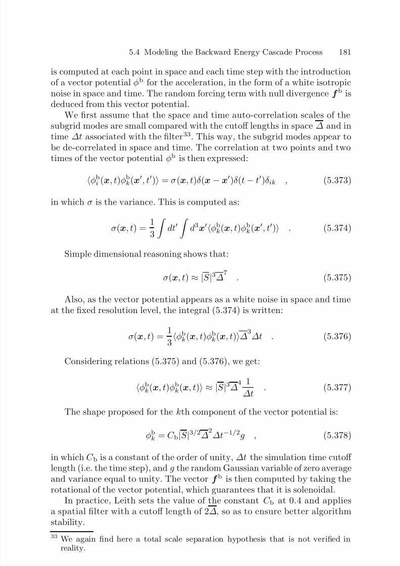
7/21/2019 Large Eddy Simulation for Incompressible Flows
http://slidepdf.com/reader/full/large-eddy-simulation-for-incompressible-flows 203/573
5.4 Modeling the Backward Energy Cascade Process 181
is computed at each point in space and each time step with the introductionof a vector potential φb for the acceleration, in the form of a white isotropicnoise in space and time. The random forcing term with null divergence f b isdeduced from this vector potential.
We first assume that the space and time auto-correlation scales of thesubgrid modes are small compared with the cutoff lengths in space ∆ and intime ∆t associated with the filter33. This way, the subgrid modes appear tobe de-correlated in space and time. The correlation at two points and twotimes of the vector potential φb is then expressed:
φbi (x, t)φb
k(x, t) = σ(x, t)δ (x − x)δ (t − t)δ ik , (5.373)
in which σ is the variance. This is computed as:
σ(x, t) = 1
3
dt
d3xφb
k(x, t)φbk(x, t) . (5.374)
Simple dimensional reasoning shows that:
σ(x, t) ≈ |S |3∆7
. (5.375)
Also, as the vector potential appears as a white noise in space and timeat the fixed resolution level, the integral (5.374) is written:
σ(x, t) = 1
3φbk(x, t)φb
k(x, t)∆3
∆t . (5.376)
Considering relations (5.375) and (5.376), we get:
φbk(x, t)φb
k(x, t)
≈ |S
|3∆
4 1
∆t
. (5.377)
The shape proposed for the kth component of the vector potential is:
φbk = C b|S |3/2∆
2∆t−1/2g , (5.378)
in which C b is a constant of the order of unity, ∆t the simulation time cutoff length (i.e. the time step), and g the random Gaussian variable of zero averageand variance equal to unity. The vector f b is then computed by taking therotational of the vector potential, which guarantees that it is solenoidal.
In practice, Leith sets the value of the constant C b at 0.4 and appliesa spatial filter with a cutoff length of 2∆, so as to ensure better algorithmstability.
33 We again find here a total scale separation hypothesis that is not verified inreality.
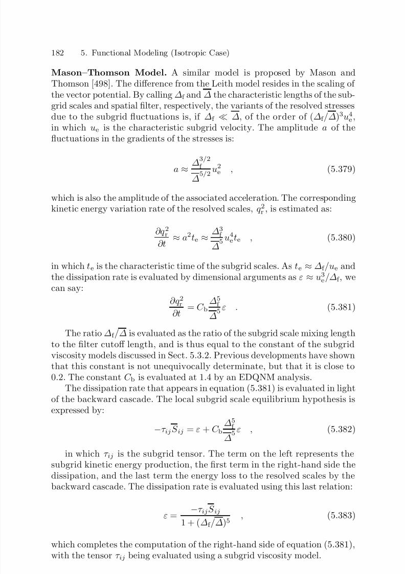
7/21/2019 Large Eddy Simulation for Incompressible Flows
http://slidepdf.com/reader/full/large-eddy-simulation-for-incompressible-flows 204/573
182 5. Functional Modeling (Isotropic Case)
Mason–Thomson Model. A similar model is proposed by Mason andThomson [498]. The difference from the Leith model resides in the scaling of the vector potential. By calling ∆f and ∆ the characteristic lengths of the sub-grid scales and spatial filter, respectively, the variants of the resolved stressesdue to the subgrid fluctuations is, if ∆f ∆, of the order of (∆f /∆)3u4
e ,in which ue is the characteristic subgrid velocity. The amplitude a of thefluctuations in the gradients of the stresses is:
a ≈ ∆3/2f
∆5/2
u2e , (5.379)
which is also the amplitude of the associated acceleration. The correspondingkinetic energy variation rate of the resolved scales, q 2r , is estimated as:
∂q 2r∂t
≈ a2te ≈ ∆3f
∆5 u4
e te , (5.380)
in which te is the characteristic time of the subgrid scales. As te ≈ ∆f /ue andthe dissipation rate is evaluated by dimensional arguments as ε ≈ u3
e/∆f , wecan say:
∂q 2r∂t
= C b ∆5f
∆5 ε . (5.381)
The ratio ∆f /∆ is evaluated as the ratio of the subgrid scale mixing lengthto the filter cutoff length, and is thus equal to the constant of the subgridviscosity models discussed in Sect. 5.3.2. Previous developments have shownthat this constant is not unequivocally determinate, but that it is close to0.2. The constant C b is evaluated at 1.4 by an EDQNM analysis.
The dissipation rate that appears in equation (5.381) is evaluated in light
of the backward cascade. The local subgrid scale equilibrium hypothesis isexpressed by:
−τ ijS ij = ε + C b∆5
f
∆5 ε , (5.382)
in which τ ij is the subgrid tensor. The term on the left represents thesubgrid kinetic energy production, the first term in the right-hand side thedissipation, and the last term the energy loss to the resolved scales by thebackward cascade. The dissipation rate is evaluated using this last relation:
ε = −τ ijS ij
1 + (∆f /∆)5 , (5.383)
which completes the computation of the right-hand side of equation (5.381),with the tensor τ ij being evaluated using a subgrid viscosity model.
7/21/2019 Large Eddy Simulation for Incompressible Flows
http://slidepdf.com/reader/full/large-eddy-simulation-for-incompressible-flows 205/573
5.4 Modeling the Backward Energy Cascade Process 183
This equation can be re-written as:
∂q 2r∂t = σ
2
a ∆t , (5.384)
in which σ2a is the sum of the variances of the acceleration component am-
plitudes. From the equality of the two relations (5.381) and (5.384), we cansay:
σ2a = C b
∆5f
∆5
ε
∆t . (5.385)
The vector potential scaling factor a and σ2a are related by:
a = σ2a
∆tte
. (5.386)
To complete the model, we now have to evaluate the ratio of the subgridscale characteristic time to the time resolution scale. This is done simply byevaluating the characteristic time te from the subgrid viscosity ν sgs computedby the model used, to reflect the cascade:
te = ∆2
f
ν sgs
, (5.387)
which completes the description of the model, since the rest of the procedureis the same as what Leith defined.
Schumann Model. Schumann proposed a stochastic model for subgrid ten-sor fluctuations that originate the backward cascade of kinetic energy [654].The subgrid tensor τ is represented as the sum of a turbulent viscosity modeland a stochastic part Rst:
τ ij = ν sgsS ij +
2
3 q 2
sgsδ ij + Rstij . (5.388)
The average random stresses Rstij are zero:
Rstij = 0 . (5.389)
They are defined as:
Rstij = γ m
vivj − 2
3q 2sgsδ ij
, (5.390)
in which γ m is a parameter and vi a random velocity. From dimensionalarguments, we can define this as:
vi =
2q 2sgs
3 gi , (5.391)

7/21/2019 Large Eddy Simulation for Incompressible Flows
http://slidepdf.com/reader/full/large-eddy-simulation-for-incompressible-flows 206/573
184 5. Functional Modeling (Isotropic Case)
in which gi is a white random number in space and has a characteristiccorrelation time τ v:
gi = 0 , (5.392)
gi(x, t)gj(x, t) = δ ijδ (x − x) exp(|t − t|/τ v) . (5.393)
The vi field is made solenoidal by applying a projection step. We notethat the time scale τ v is such that:
τ v
q 2sgs/∆ ≈ 1 . (5.394)
The parameter γ m determines the portion of random stresses that gen-
erate the backward cascade. Assuming that only the scales belonging to theinterval [kc, nkc] are active, for a spectrum of slope of −m we get:
γ 2m =
nkc
kc
k−2mdk ∞kc
k−2mdk
= 1 − n1−2m . (5.395)
For n = 2 and m = 5/3, we get γ m = 0.90. The subgrid kinetic energy
q 2sgs is evaluated from the subgrid viscosity model.
Stochastic Localized Dynamic Model. A localized dynamic procedureincluding a stochastic forcing term was proposed by Carati et al. [101]. Thecontribution of the subgrid terms in the momentum equation appears hereas the sum of a subgrid viscosity model, denoted C dβ ij using the notation of Sect. 5.3.3, which models the energy cascade, and a forcing term denoted f :
∂τ ij∂xj
= ∂C dβ ij
∂xj+ f i . (5.396)
The β ij term can be computed using any subgrid viscosity model. Theforce f is chosen in the form of a white noise in time with null divergence inspace. The correlation of this term at two points in space and two times istherefore expressed:
f i(x, t)f j(x, t) = A2(x, t)H ij(x − x)δ (t − t) . (5.397)
The statistical average here is an average over all the realizations of f conditioned by a given velocity field u(x, t). The factor A2 is such that
H ii(0) = 1. Since a stochastic term has been introduced into the subgridmodel, the residual E ij on which the dynamic procedure for computing theconstant C d is founded also possesses a stochastic nature. This property willtherefore be shared by the dynamically computed constant, which is not ac-ceptable. To find the original properties of the dynamic constant, we takea statistical average of the residual, denoted E ij, which gets rid of the
7/21/2019 Large Eddy Simulation for Incompressible Flows
http://slidepdf.com/reader/full/large-eddy-simulation-for-incompressible-flows 207/573
5.4 Modeling the Backward Energy Cascade Process 185
random terms. The constant of the subgrid viscosity model is computed bya localized dynamic procedure based on the statistical average of the residual,which is written:
E ij = Lij + C dβ ij − C dαij . (5.398)
The amplitude of the random forcing term can also be computed dynam-ically. To bring out the non-zero contribution of the stochastic term in thestatistical average, we base this new procedure on the resolved kinetic energybalance at the level of the test filter Q2
r = uiui/2. The evolution equation of this quantity is obtained in two different forms (only the pertinent terms aredetailed, the others are symbolized):
∂Q2r
∂t = ... − ui ∂
∂xj(C dαij + P δ ij) + E F , (5.399)
∂Q2r
∂t = ... − ui ∂
∂xj
C dβ ij + Lij + pδ ij
+ E f . (5.400)
The pressure terms P and p are in equilibrium with the velocity fields
u and u, respectively. The quantities E F and E
f are the backward cascade
energy injections associated, respectively, with the forcing term F computeddirectly at the level of the test filter, and with the forcing term f computedat the first level and then filtered. The difference between equations (5.399)and (5.400) leads to:
Z ≡ E F − E f − g = 0 , (5.401)
in which the fully known term g is of the form:
g =
ui
∂
∂xj C dαij + P δ ij −
C dβ ij − Lij −
pδ ij
. (5.402)
The quantity Z plays a role for the kinetic energy that is analogous tothe residual E ij for the momentum. Minimizing the quantity
Z = Z 2 (5.403)
can thus serve as a basis for defining a dynamic procedure for evaluating thestochastic forcing.
To go any further, the shape of the f term has to be specified. To simplifythe use, we assume that the correlation length of f is small compared withthe cutoff length ∆. The function f thus appears as de-correlated in space,which is reflected by:
E f = 1
2A2(x, t) . (5.404)

7/21/2019 Large Eddy Simulation for Incompressible Flows
http://slidepdf.com/reader/full/large-eddy-simulation-for-incompressible-flows 208/573
186 5. Functional Modeling (Isotropic Case)
In order to be able to calculate E f dynamically, we assume that the back-ward cascade is of equal intensity at the two filtering levels considered, i.e.
E f = E F . (5.405)
Also, since f is de-correlated at the ∆ scale, we assume:
E f E f = E F , (5.406)
which makes it possible to change relation (5.401) to become
Z = E F − g . (5.407)
We now choose f in the form:
f i = P ij(Aej) , (5.408)
in which ej is a random isotropic Gaussian function, A a dimensioned con-stant that will play the same role as the subgrid viscosity model constant,and P ij the projection operator on a space of zero divergence. We have therelations:
ei(x, t)
= 0 , (5.409)
ei(x, t)ei(x, t) = 1
3δ ijδ (t − t)δ (x − x) . (5.410)
Considering (5.408), (5.410) and (5.404), we get:
E f = 1
2A2 =
1
3A2 . (5.411)
The computation of the model is completed by evaluating the constant
A by a constrained localized dynamic procedure based on minimizing the
functional (5.403), which can be re-written in the form:
Z [A] =
A2
3 − g
2
. (5.412)
7/21/2019 Large Eddy Simulation for Incompressible Flows
http://slidepdf.com/reader/full/large-eddy-simulation-for-incompressible-flows 209/573
6. Functional Modeling:Extension to Anisotropic Cases
6.1 Statement of the Problem
The developments of the previous chapters are all conducted in the isotropicframework, which implies that both the filter used and the flow are isotropic.They can be extended to anisotropic or inhomogeneous cases only by localiz-ing the statistical relations in space and time and introducing heuristic pro-cedures for adjusting the models. But when large-eddy simulation is appliedto inhomogeneous flows, we very often have to use anisotropic grids, whichcorrespond to using a anisotropic filter. So there are two factors contributingto the violation of the hypotheses underlying the models presented so far: fil-ter anisotropy (respectively inhomogeneity) and flow anisotropy (respectively
inhomogeneity).This chapter is devoted to extensions of the modeling to anisotropic cases.
Two situations are considered: application of a anisotropic homogeneous filterto an isotropic homogeneous turbulent flow (Sect. 6.2), and application of anisotropic filter to an anisotropic flow (Sect. 6.3).
6.2 Application of Anisotropic Filter to Isotropic Flow
The filters considered in the following are anisotropic in the sense that thefilter cutoff length is different in each direction of space. The different typesof anisotropy possible for Cartesian filtering cells are represented in Fig. 6.1.
In order to use an anisotropic filter to describe an isotropic flow, we arefirst required to modify the subgrid models, because theoretical work andnumerical experiments have shown that the resolved fields and the subgridthus defined are anisotropic [368]. For example, for a mesh cell with an aspectratio ∆2/∆1 = 8, ∆3/∆1 = 4, the subgrid stresses will differ from their valuesobtained with an isotropic filter by about ten percent. It is very important to
note, though, that this anisotropy is an artifact due to the filter but that thedynamic of the subgrid scales still corresponds that of isotropic homogeneousturbulence.
On the functional modeling level, the problem is in determining the char-acteristic length that has to be used to compute the model.

7/21/2019 Large Eddy Simulation for Incompressible Flows
http://slidepdf.com/reader/full/large-eddy-simulation-for-incompressible-flows 210/573
188 6. Functional Modeling: Extension to Anisotropic Cases
Fig. 6.1. Different types of filtering cells. Isotropic cell (on the left): ∆1 = ∆2 = ∆3;pancake-type anisotropic cell (center): ∆1 ∆2 ≈ ∆3; cigar-type anisotropic cell(right): ∆1 ≈ ∆2 ∆3.
Two approaches are available:
– The first consists in defining a single length scale for representing the filter.This lets us keep models analogous to those defined in the isotropic case,
using for example scalar subgrid viscosities for representing the forwardcascade process. This involves only a minor modification of the subgridmodels since only the computation of the characteristic cutoff scale is mod-ified. But it should be noted that such an approach can in theory be validonly for cases of low anisotropy, for which the different cutoff lengths areof the same order of magnitude.
– The second approach is based on the introduction of several characteristiclength scales in the model. This sometimes yields major modifications inthe isotropic models, such as the definition of tensorial subgrid viscosities
to represent the forward cascade process. In theory, this approach takes thefilter anisotropy better into account, but complicates the modeling stage.
6.2.1 Scalar Models
These models are all of the generic form ∆ = ∆(∆1, ∆2, ∆3). We presenthere:
1. Deardorff’s original model and its variants (p. 189). These forms are em-
pirical and have no theoretical basis. All we do is simply to show that theyare consistent with the isotropic case, i.e. ∆ = ∆1 when ∆1 = ∆2 = ∆3.2. The model of Scotti et al. (p. 189), which is based on a theoretical analy-
sis considering a Kolmogorov spectrum with an anisotropic homogeneousfilter. This model makes a complex evaluation possible of the filter cutoff length, but is limited to the case of Cartesian filtering cells.

7/21/2019 Large Eddy Simulation for Incompressible Flows
http://slidepdf.com/reader/full/large-eddy-simulation-for-incompressible-flows 211/573
6.2 Application of Anisotropic Filter to Isotropic Flow 189
Deardorff’s Proposal. The method most widely used today is withoutdoubt the one proposed by Deardorff [172], which consists in evaluating thefilter cutoff length as the cube root of the volume V Ω of the filtering cell Ω .Or, in the Cartesian case:
∆(x) =
∆1(x)∆2(x)∆3(x)1/3
, (6.1)
in which ∆i(x) is the filter cutoff length in the ith direction of space atposition x.
Extensions of Deardorff’s Proposal. Simple extensions of definition (6.1)are often used, but are limited to the case of Cartesian filtering cells:
∆(x) =
(∆
21(x) + ∆
22(x) + ∆
23(x))/3 , (6.2)
∆(x) = max
∆1(x), ∆2(x), ∆3(x)
. (6.3)
Another way to compute the characteristic length on a strongly non-uniform mesh, which prevents the occurrence of large values of subgrid vis-cosity, was proposed by Arad [16]. It relies on the use of the harmonic meanof the usual length scales:
∆(x) =
∆1(x) ∆2(x) ∆3(x)1/3
, (6.4)
with
∆i(x) =
(∆i(x))−ω + (∆M
i )−ω−1/ω
, i = 1, 2, 3 , (6.5)
where ∆M i is a prescribed bound for ∆i(x), and ω > 0.
Proposal of Scotti et al. More recently, Scotti, Meneveau, and Lilly [664]proposed a new definition of ∆ based on an improved estimate of the dissi-pation rate ε in the anisotropic case. The filter is assumed to be anisotropicbut homogeneous, i.e. the cutoff length is constant in each direction of space.
We define ∆max = max(∆1, ∆2, ∆3). Aspect ratios of less than unity,constructed from the other two cutoff lengths with respect to ∆max, aredenoted a1 and a2
1. The form physically sought for the anisotropy correction
is:∆ = ∆isof (a1, a2) , (6.6)
in which ∆iso is Deardorff’s isotropic evaluation computed by relation (6.1).
1 For example, by taking ∆max = ∆1, we get a1 = ∆2/∆1 and a2 = ∆3/∆1.
7/21/2019 Large Eddy Simulation for Incompressible Flows
http://slidepdf.com/reader/full/large-eddy-simulation-for-incompressible-flows 212/573
190 6. Functional Modeling: Extension to Anisotropic Cases
Using the approximation:
ε
= ∆
2
2S ijS ij
3/2 , (6.7)
and the following equality, which is valid for a Kolmogorov spectrum,
S ijS ij = ε2/3 K 02π
| G(k)|2k−5/3d3k , (6.8)
where G(k) is the kernel of the anisotropic filter considered, after calculationwe get:
∆ =
K 02π
|
G(k)|2k−5/3d3k
−3/4
. (6.9)
Considering a sharp cutoff filter, we get the following approximate relationby integrating equation (6.9):
f (a1, a2) = cosh
4
27 [(ln a1)2 − ln a1 ln a2 + (ln a2)2] . (6.10)
It is interesting to note that the dynamic procedure (see Sect. 5.3.3) for thecomputation of the Smagorinsky constant can be interpreted as an implicitway to compute the f (a1, a2) function [663]. Introducing the subgrid mixinglength ∆f , the Smagorinsky model reads
ν sgs = ∆2f |S | (6.11)
= C d∆2iso|S | (6.12)
= (C S∆isof (a1, a2))2|S | , (6.13)
where C d is the value of the constant computed using a dynamic procedure,and C S the theoretical value of the Smagorinsky constant evaluated throughthe canonical analysis. A trivial identification leads to:
f (a1, a2) = C d/C S . (6.14)
This interpretation is meaningful for positive values of the dynamic con-stant. A variant can be derived by using the anisotropy measure f (a1, a2) in-stead of the isotropic one inside the dynamic procedure (see equation (6.12)),yielding new definitions of the tensors αij and β ij appearing in the dynamicprocedure (see Table 5.1). Taking the Smagorinsky model as an example, weget:
β ij =
−2(∆isof (a1, a2))2
|S
|S ij , αij =
−2(∆isof (a1,a2))2
|S
|S ij , (6.15)
where f (a1, a2) and f (a1,a2) are the anisotropy measures associated to thefirst and second filtering levels, respectively. The corresponding formulationof the f function is now:
f (a1, a2) =
C d/(C S∆iso) . (6.16)
7/21/2019 Large Eddy Simulation for Incompressible Flows
http://slidepdf.com/reader/full/large-eddy-simulation-for-incompressible-flows 213/573
6.2 Application of Anisotropic Filter to Isotropic Flow 191
6.2.2 Batten’s Mixed Space-Time Scalar Estimator
It was shown in Sect. 2.1.3 that spatial filtering induces a time filtering. In
a reciprocal manner, enforcing a time-frequency cutoff leads to the defini-tion of an intrinsic spatial cutoff length. To account for that phenomenon,Batten [49] defines the cutoff length as
∆(x) = 2 max
∆1(x), ∆2(x), ∆3(x),
q 2sgs∆t
, (6.17)
where ∆t and q 2sgs are the time step of the simulation and the subgridkinetic energy, respectively. The subgrid kinetic energy can be computed
solving an prognostic transport equation (p. 128) or one of the methodsdiscussed in Sect. 9.2.3.
6.2.3 Tensorial Models
The tensorial models presented in the following are constructed empirically,with no physical basis. They are justified only by intuition and only forhighly anisotropic filtering cells of the cigar type, for example (see Fig. 6.1).Representing the filter by a single and unique characteristic length is no longer
relevant. The filter’s characteristic scales and their inclusion in the subgridviscosity model are determined intuitively. Two such models are described:
1. The model of Bardina et al. (p. 191), which describes the geometry of thefiltering cell by means of six characteristic lengths calculated from theinertia tensor of the filtering cell. This approach is completely general andis a applicable to all possible types of filtering cells (Cartesian, curvilinear,and other), but entrains a high complexification in the subgrid models.
2. The model of Zahrai et al. (p. 192), which is applicable only to Cartesiancells and is simple to include in the subgrid viscosity models.
Proposal of Bardina et al.
Definition of a Characteristic Tensor. These authors [39] propose replacingthe isotropic scalar evaluation of the cutoff length associated with the gridby an anisotropic tensorial evaluation linked directly to the filtering cell ge-ometry: V (x) = (∆1(x)∆2(x)∆3(x)). To do this, we introduce the momentsof the inertia tensor I associated at each point x:
I ij(x) =
1
V (x) V xixjdV . (6.18)
Since the components of the inertia tensor are homogeneous at the squareof a length, the tensor of characteristic lengths is obtained by taking thesquare root of them. In the case of a pancake filtering cell aligned with the

7/21/2019 Large Eddy Simulation for Incompressible Flows
http://slidepdf.com/reader/full/large-eddy-simulation-for-incompressible-flows 214/573
192 6. Functional Modeling: Extension to Anisotropic Cases
axes of the Cartesian coordinate system, we get the diagonal matrix:
I ij = 23 ∆
2
1 0 00 ∆22 0
0 0 ∆23
. (6.19)
Application to the Smagorinsky Model. As we model only the anisotropic partof the subgrid tensor, the tensor I is decomposed into the sum of a sphericalterm I i and an anisotropic term I d:
I ij = I iδ ij + ( I ij − I iδ ij) = I iδ ij + I dij , (6.20)
with
I i = 1
3 I kk =
1
3(∆
21 + ∆
22 + ∆
23) . (6.21)
Modifying the usual Smagorinsky model, the authors finally propose thefollowing anisotropic tensorial model for deviator of the subgrid tensor τ :
τ ij − 1
3τ kkδ ij = C 1 I i|S |S ij
+ C 2|S | I ikS kj + I jkS ki − 13 I lkS klδ ij (6.22)
+ C 3|S | I i
I ik I jlS kl − 1
3 I mk I mlS klδ ij
,
in which C 1, C 2 and C 3 are constants to be evaluated.
Proposal of Zahrai et al.
Principle. Zahrai et al. [795] proposed conserving the isotropic evaluation of the dissipation rate determined by Deardorff and further considering thatthis quantity is constant over each mesh cell:
ε =
∆1(x)∆2(x)∆3(x)2/3 2S ijS ij3/2 . (6.23)
On the other hand, when deriving the subgrid model, we consider thatthe filter’s characteristic length in each direction is equal to the cutoff lengthin that direction. This procedure calls for the definition of a tensorial modelfor the subgrid viscosity.
Application to the Smagorinsky model. In the case of the Smagorinsky model,we get for component k:
(ν sgs)k = C 1(∆1∆2∆3)2/9(∆k)4/32S ijS ij3/2 , (6.24)
where C 1 is a constant.
7/21/2019 Large Eddy Simulation for Incompressible Flows
http://slidepdf.com/reader/full/large-eddy-simulation-for-incompressible-flows 215/573
6.3 Application of an Isotropic Filter to a Shear Flow 193
6.3 Application of an Isotropic Filter to a Shear Flow
We will now be examining the inclusion of subgrid scale anisotropy in the
functional models.The first part of this section presents theoretical results concerning sub-
grid scale anisotropy and the interaction mechanisms between the large andsmall scales in this case. These results are obtained either by the EDQNMtheory or by asymptotic analysis of the triadic interactions.
The second part of the section describes the modifications that have beenproposed for functional type subgrid models. Only models for the forwardenergy cascade will be presented, because no model for the backward cascadehas yet been proposed in the anisotropic case.
6.3.1 Phenomenology of Inter-Scale Interactions
Anisotropic EDQNM Analysis. Aupoix [24] proposes a basic analysis of the effects of anisotropy in the homogeneous case using Cambon’s anisotropicEDQNM model. The essential details of this model are given in Appendix B.
The velocity field u is decomposed as usual into average part u anda fluctuating part u:
u =
u
+ u . (6.25)
To study anisotropic homogeneous flows, we define the spectral tensor
Φij(k) = u∗i (k) uj(k) , (6.26)
which is related to the double correlations in the physical space by the rela-tion:
uiuj(x) =
Φij(k)d3k . (6.27)
Starting with the Navier–Stokes equations, we obtain the evolution equa-tion (see Appendices A and B):
∂
∂t + 2νk2
Φij(k) +
∂ ui∂xl
Φjl(k) + ∂ uj
∂xlΦil(k)
− 2∂ ul∂xm
(kiΦjm(k) + kjΦmi(k))
− ∂ ul∂xm
∂
∂km(klΦij(k))
= P il(k)T lj(k) + P jl(k)T ∗li(k) , (6.28)

7/21/2019 Large Eddy Simulation for Incompressible Flows
http://slidepdf.com/reader/full/large-eddy-simulation-for-incompressible-flows 216/573
194 6. Functional Modeling: Extension to Anisotropic Cases
where
T ij(k) = kl ui(k)ul( p)uj(
−k
− p)
d3 p , (6.29)
and
P ij(k) =
δ ij − kikj
k2
, (6.30)
and where the * designates the complex conjugate number. We then simplifythe equations by integrating the tensor Φ on spheres of radius k=cste:
φij
(k) = Φij
(k)dA(k) , (6.31)
and obtain the evolution equations:∂
∂t + 2νk2
φij(k) = −∂ ui
∂xkφjl(k) − ∂ uj
∂xlφil(k)
+ P lij(k) + S lij(k) + P nlij (k) + S nl
ij (k) ,
(6.32)
where the terms P l, S l, P nl and S nl are the linear pressure, linear transfer,non-linear pressure, and non-linear transfer contributions, respectively. Thelinear terms are associated with the action of the average velocity gradient,and the non-linear terms with the action of the turbulence on itself.
The expression of these terms and their closure by the anisotropicEDQNM approximation are given in Appendix B. Using these relations,Aupoix derives an expression for the interaction between the modes cor-responding to wave numbers greater than a given cutoff wave number kc (i.e.
the small or subgrid scales) and those associated with small wave numberssuch that k ≤ kc (i.e. the large or resolved scales). To obtain a simple ex-pression for the coupling among the different scales by the non-linear termsP nl and S nl, we adopt the hypothesis that there exists a total separation of scales (in the sense defined in Sect. 5.3.2) between the subgrid and resolvedmodes, so that we can obtain the following two asymptotic forms:
P nlij (k) = − 32
175k4
∞kc
Θ0 pp [10 + a( p)] E 2( p)H ij( p)
p2 dp
+ 16105
k2E (k) ∞kc
Θ0 pp (a( p) + 3) p ∂ ∂p
(E ( p)H ij( p))
+E ( p)H ij( p)
5 a( p) + 3 + p
∂a( p)
∂p
dp , (6.33)
7/21/2019 Large Eddy Simulation for Incompressible Flows
http://slidepdf.com/reader/full/large-eddy-simulation-for-incompressible-flows 217/573
6.3 Application of an Isotropic Filter to a Shear Flow 195
S nlij (k) = 2k4
∞kc
Θ0 ppE 2( p)
p2
14
15
1
3δ ij + 2H ij( p)
+
8
25a( p)H ij( p)
dp
− 2k2φij(k) 115 ∞kc
Θ0 pp 5E ( p) + p ∂E ( p)∂p
dp
− 2k2E (k)
∞kc
Θ0 pp
2
15
5E ( p)H ij( p) + p
∂
∂p(E ( p)H ij( p))
+E ( p)H ij( p)
8
15(a( p) + 3) +
8
25a( p)
dp , (6.34)
where E (k) is the energy spectrum, defined as:
E (k) = 12 φll(k) , (6.35)
and H ij(k) the anisotropy spectrum:
H ij(k) = φij(k)
2E (k) − 1
3δ ij . (6.36)
It is easily verified that, in the isotropic case, H ij cancels out by con-struction. The function a(k) is a structural parameter that represents theanisotropic distribution on the sphere of radius k, and Θkpq the characteris-tic relaxation time evaluated by the EDQNM hypotheses. The expression of this term is given in Appendix B.
These equations can be simplified by using the asymptotic value of thestructural parameter a(k). By taking a(k) = −4.5, we get:
P nlij (k) + S nl
ij (k) = k4
∞kc
Θ0 ppE 2( p)
p2
28
45δ ij − 368
175H ij( p)
dp
− 2k2φij(k)
1
15 ∞
kc
Θ0 pp 5E ( p) + p∂E ( p)
∂p dp
+ k2E (k) ∞kc
Θ0 pp
1052
525 E ( p)H ij( p)
− 52
105
∂
∂p (E ( p)H ij( p))
dp . (6.37)
From this equation, it can be seen that the anisotropy of the small scalestakes on a certain importance. In a case where the anisotropic spectrum hasthe same (resp. opposite) sign for the small scales as it does for the large, the
term in k4
constitutes a return of energy that has the effect of a return towardisotropy (resp. departure from isotropy), and the term in k2E (k) representsan backward energy cascade associated with an increasing anisotropy (resp.a return to isotropy). Lastly, the term in k2φij(k) is a term of isotropicdrainage of energy to the large scales by the small, and represents here theenergy cascade phenomenon modeled by the isotropic subgrid models.

7/21/2019 Large Eddy Simulation for Incompressible Flows
http://slidepdf.com/reader/full/large-eddy-simulation-for-incompressible-flows 218/573
196 6. Functional Modeling: Extension to Anisotropic Cases
Asymptotic Analysis of Triadic Interactions. Another analysis of inter-scale interactions in the isotropic case is the asymptotic analysis of triadicinteractions [74, 785].
The evolution equation of the Fourier mode u(k) is written in the symbolicform:
∂ u(k)
∂t = u(k) = [u(k)]nl + [u(k)]vis , (6.38)
where [ u(k)]nl and [ u(k)]vis represent, respectively, the non-linear terms as-sociated with the convection and pressure, and the linear term associatedwith the viscous effects, defined as:
[ u(k)]nl = −i p
u( p)⊥k (k · u(k − p)) , (6.39)
with
ui( p)⊥k =
δ ij − kikj
k2
uj( p) , (6.40)
[ u(k)]vis =
−νk2
u(k) . (6.41)
The evolution equation of the modal energy, e(k) = u(k) · u∗(k), is of theform:
∂e(k)
∂t = u(k) · u∗(k) + cc = [e(k)]nl + [e(k)]vis , (6.42)
with
[e(k)]nl = −i p
u∗(k) ·
u( p)
[k ·
u(k − p)] + cc , (6.43)
[e(k)]vis = −2νk2e(k) , (6.44)
where the symbol cc designates the complex conjugate number of the termthat precedes it. The non-linear energy transfer term brings in three wavevectors (k, p, q = k − p) and is consequently a linear sum of non-linear triadicinteractions. We recall (see Sect. 5.1.2) that the interactions can be classifiedinto various categories ranging from local interactions, for which the normsof the three wave vectors are similar (i.e. k
∼ p
∼q ), to distant interactions
for which the norm of one of the wave vectors is very small compared withthe other two (for example k p ∼ q ). The local interactions thereforecorrespond to the inter-scale interactions of the same size and the distantinteractions to the interactions between a large scale and two small scales.
7/21/2019 Large Eddy Simulation for Incompressible Flows
http://slidepdf.com/reader/full/large-eddy-simulation-for-incompressible-flows 219/573
6.3 Application of an Isotropic Filter to a Shear Flow 197
Also, any interaction that introduces a (k, p, q) triad that does not verify therelation k ∼ p ∼ q is called a non-local interaction.
In the following, we will be analyzing an isolated distant triadic interactionassociated with three modes: k, p and q. We adopt the configuration k
p ∼ q and assume that k is large scale located in the energetic portion of thespectrum. An asymptotic analysis shows that:
[ u(k)]nl = O(δ ) , (6.45)
[ u( p)]nl = −i
u∗(q)
p ·
u∗(k)
+ O(δ ) , (6.46)
[ u(q)]nl = −i u∗
( p) p · u∗
(k)+ O(δ ) , (6.47)
where δ is the small parameter defined as
δ = k
p 1 .
The corresponding energy transfer analysis leads to the following rela-tions:
[e(k
)]nl = O(δ ) , (6.48)
[e( p)]nl = − [e(q)]nl = i u( p) · u(q) [ p · u(k)] + cc + O(δ ) . (6.49)
Several remarks can be made:
– The interaction between large and small scales persists in the limit of theinfinite Reynolds numbers. Consistently with the Kolmogorov hypotheses,these interactions occur with no energy transfer between the large andsmall scales. Numerical simulations have shown that the energy transfers
are negligible between two modes separated by more than two decades.– The variation rate of the high frequencies u( p) and u(q) is directly pro-
portional to the amplitude of the low-frequency mode u(k). This impliesthat the strength of the coupling with the low-frequency modes increaseswith the energy of the modes.
Moreover, complementary analysis shows that, for modes whose wave-length is of the order of the Taylor micro-scale λ defined as (see AppendixA):
λ = u2∂u
∂x
2, (6.50)
7/21/2019 Large Eddy Simulation for Incompressible Flows
http://slidepdf.com/reader/full/large-eddy-simulation-for-incompressible-flows 220/573
198 6. Functional Modeling: Extension to Anisotropic Cases
the ratio between the energy transfers due to the distant interactions andthose due to the local interactions vary as:
[e(kλ)]distant
[e(kλ)]local
∼ Re11/6λ , (6.51)
where Reλ is the Reynolds number referenced to the Taylor micro-scale andthe velocity fluctuation u. This relation shows that the coupling increaseswith the Reynolds number, with the result that an anisotropic distributionof the energy at the low frequencies creates an anisotropic forcing of the highfrequencies, leading to a deviation from isotropy of these high frequencies.
A competitive mechanism exists that has an isotropy reduction effect
at the small scales. This is the energy cascade associated with non-localtriadic interactions that do not enter into the asymptotic limit of the distantinteractions.
For a wave vector of norm k, the ratio of the characteristic timesτ (k)cascade and τ (k)distant, associated respectively with the energy transferof the cascade mechanism and that due to the distant interactions, is evalu-ated as:
τ (k)cascade
τ (k)distant∼ constant × (k/kinjection)11/6 , (6.52)
where kinjection is the mode in which the energy injection occurs in thespectrum. So we see that the distant interactions are much faster than theenergy cascade. Also, the first effect of a sudden imposition of large scaleanisotropy will be to anisotropize the small scales, followed by competitionbetween the two mechanisms. The dominance of one of the two depends ona number of factors, such as the separation between the k and kinjection scales,or the intensity and coherence of the anisotropy at the large scale.
Numerical simulations [785] performed in the framework of homogeneousturbulence have shown a persistence of anisotropy at the small scales. How-
ever, it should be noted that this anisotropy is detected only on statisticalmoments of the velocity field of order three or more, with first- and second-order moments being isotropic.
6.3.2 Anisotropic Models: Scalar Subgrid Viscosities
The subgrid viscosity models presented in this section have been designed toalleviate the problem observed with basic subgrid viscosities, i.e. to preventthe occurance of too high dissipation levels in shear flows, which are known
to have disastrous effects in near-wall regions.2
The models presented beloware:
2 Problems encountered in free shear flows are usually less important, since largescales are often driven by inviscid instabilities, while the existence of a criticalReynolds number may lead to relaminarization if the subgrid viscosity is toohigh.
7/21/2019 Large Eddy Simulation for Incompressible Flows
http://slidepdf.com/reader/full/large-eddy-simulation-for-incompressible-flows 221/573
6.3 Application of an Isotropic Filter to a Shear Flow 199
1. WALE model by Nicoud and Ducros (p. 199), which is built to recoverthe expected asymptotic behavior in the near-wall region in equilibriumturbulent boundary layers on fine grids, without any additional dampingfunction.
2. Casalino–Jacob Weighted Gradient Model (p. 199), which is based ona modification of the of the Smagorinsky constant to make it sensitive tothe mean shear stresses, rendering it more local in terms of wave number.
3. Models based on the idea of separating the field into an isotropic partand inhomogeneous part (p. 200), in order to be able to isolate the contri-bution of the mean field in the computation of the subgrid viscosity, formodels based on the large scales, and thereby better localize the infor-mation contained in these models by frequency. This technique, however,
is applicable only to flows whose mean velocity profile is known or canbe computed on the fly.
Wall-Adapting Local Eddy-Viscosity Model. It has been seen before(p. 159) that most subgrid viscosity models do not exhibit the correct behav-ior in the vicinity of solid walls in equilibrium boundary layers on fine grids,resulting in a too high damping of fluctuations in that region and to a wrongprediction of the skin friction. The common way to alleviate this problemis to add a damping function, which requires the distance to the wall and
the skin friction as input parameters, leading to complex implementation is-sues. Another possibility is to use self-adpative models, which involve a largeralgorithmic complexity.
An elegant solution to solve the near-wall region problem on fine grids isproposed by Nicoud and Ducros [567], who found a combination of resolvedvelocity spatial derivatives that exhibits the expected asymptotic behaviorν sgs ∝ z+3
, where z+ is the distance to the wall expressed in wall units.The subgrid viscosity is defined as
ν sgs = (C w∆)2 S d
ijS d
ij3/2S ijS ij
5/2+S dijS dij
5/4 , (6.53)
with C w = 0.55 − 0.60 and
S dij = S ikS kj + Ω ikΩ kj − 1
3
S mnS mn − Ω mnΩ mn
δ ij . (6.54)
This model also possesses the interesting property that the subgrid viscos-ity vanishes when the flow is two-dimensional, in agreement with the physical
analysis.
Weighted Gradient Subgrid Viscosity Model. Casalino, Boudet andJacob [112] introduced a modification in the evaluation of the Smagorinskyconstant to render it sensitive to resolved gradients, with the purpose of recovering a better accuracy in shear flows.
7/21/2019 Large Eddy Simulation for Incompressible Flows
http://slidepdf.com/reader/full/large-eddy-simulation-for-incompressible-flows 222/573
200 6. Functional Modeling: Extension to Anisotropic Cases
The weighted gradient subgrid viscosity model is written as
ν sgs = (C (x, t)∆)2
|S ij
| , (6.55)
where the self-adaptive constant is equal to
C (x, t) = γC S
S ∗ijS ∗ij
S ijS ij
m/4
, (6.56)
where C S = 0.18 is the conventional Smagorinsky constant, γ and m arefree parameters and the weighted strain tensor S ∗ is defined as (withoutsummation over repeated greek indices)
S ∗αβ = W αβS αβ . (6.57)
The weighting matrix coefficients are inversely proportional to the thirdmoment of corresponding strain rate tensor coefficients:
W αβ =
S 3αβ
α,β=1,3
S 3αβ
−1
. (6.58)
The bracket operator is related to a local average. Numerical tests haveshown that (m, γ ) = (1, 3) and (3, 10) yield satisfactory results in free shearflows, the last values yielding the recovery of the theoretical behavior of thesubgrid viscosity in the vicinity of solid walls on fine meshes.
Models Based on a Splitting Technique. Subgrid viscosity models aremostly developed in the framework of the hypotheses of the canonical anal-ysis, i.e. for homogeneous turbulent flows. Experience shows that the per-formance of these models declines when they are used in an inhomogeneous
framework, which corresponds to a non-uniform average flow. One simpleidea initially proposed by Schumann [653] is to split the velocity field intoinhomogeneous and isotropic parts and to compute a specific subgrid termfor each of these parts.
In practice, Schumann proposes an anisotropic subgrid viscosity modelfor dealing with flows whose average gradient is non-zero, and in particularany flow regions close to solid walls. The model is obtained by splitting thedeviator part of the subgrid tensor τ d into one locally isotropic part and oneinhomogeneous:
τ dij = −2ν sgsS ij − S ij− 2ν asgsS ij , (6.59)
where the angle brackets . designate an statistical average, which in practiceis a spatial average in the directions of homogeneity in the solution. The co-efficients ν sgs and ν asgs are the scalar subgrid viscosities representing a locally
7/21/2019 Large Eddy Simulation for Incompressible Flows
http://slidepdf.com/reader/full/large-eddy-simulation-for-incompressible-flows 223/573
6.3 Application of an Isotropic Filter to a Shear Flow 201
isotropic turbulence and an inhomogeneous turbulence, respectively. Moinand Kim [537] and Horiuti [319] give the following definitions:
ν sgs = C 1∆2 2 S ij − S ij S ij − S ij , (6.60)
ν asgs =
C 2∆z
2
2S ijS ij , (6.61)
where C 1 and C 2 are two constants. Horiuti recommends C 1 = 0.1 and C 2= 0.254, while Moin and Kim use C 1 = C 2 = 0.254. The isotropic part isa function of the fluctuation of the viscosity gradients, so as to make sure thatthe extra-diagonal components thus predicted for the subgrid tensor cancelout on the average over time. This is consistent with the isotropic hypothesis.
The two characteristic lengths ∆ and ∆z represent the cutoff lengths forthe two types of structures, and are evaluated as:
∆(z) = (∆1∆2∆3)1/3(1 − exp(zuτ /Aν )) , (6.62)
∆z(z) = ∆3(1 − exp([zuτ /Aν ]2)) , (6.63)
where z is the distance to the solid wall, ∆3 the cutoff length in the direc-tion normal to the surface, and uτ the friction velocity at the surface (see
Sect. 10.2.1). The constant A is taken to be equal to 25.This model was initially designed for the case of a plane channel flow. Itrequires being able to compute the statistical average of the velocity field, andthus can be extended only to sheared flows exhibiting at least one direction of homogeneity, or requires the use of several statistically equivalent simulationsto perform the ensemble average [102, 108].
Sullivan et al. [698] propose a variant of it that incorporates an anisotropyfactor (so that the model constant can be varied to represent the fieldanisotropy better):
τ dij = −2ν sgsγS ij − 2ν asgsS ij . (6.64)
The authors propose computing the viscosity ν asgs as before. The ν sgs term,on the other hand, is now calculated by a model with one evolution equationfor the subgrid kinetic energy (see equation (5.119) in Chap. 5). Only thesubgrid kinetic energy production by the isotropic part is included, which isequivalent to replacing the II term in equation (5.119) with
2ν sgsγ
S ij − S ij
S ij − S ij . (6.65)
The authors evaluate the anisotropy factor from the shearing rates of thelarge and small scales. The average per plane of fluctuation homogeneity of the resolved strain rate tensor, calculated by
S =
2S ij − S ij
S ij − S ij , (6.66)

7/21/2019 Large Eddy Simulation for Incompressible Flows
http://slidepdf.com/reader/full/large-eddy-simulation-for-incompressible-flows 224/573
202 6. Functional Modeling: Extension to Anisotropic Cases
is used for evaluating the shear of the small scales. The shear of the largescales is estimated as
S = 2S ijS ij . (6.67)
The isotropy factor is evaluated as:
γ = S
S + S . (6.68)
6.3.3 Anisotropic Models: Tensorial Subgrid Viscosities
Here we describe the main models proposed in the anisotropic framework.Except for Aupoix’s spectral model, none of these take explicit account of the backward cascade mechanism. They are:
1. Aupoix’s spectral model (p. 203), which is based on the anisotropicEDQNM analysis. The interaction terms are evaluated by adopting a pre-set shape of the energy spectra and subgrid mode anisotropy. This model,which requires a great deal of computation, has the advantage of includ-
ing all the coupling mechanisms between large and small scales.2. Horiuti’s model (p. 204), which is based on an evaluation of the anisotropytensor of the subgrid modes from the equivalent tensor constructed fromthe highest frequencies in the resolved field. This tensor is then used tomodulate the subgrid viscosity empirically in each direction of space. Thisis equivalent to considering several characteristic velocity scales for rep-resenting the subgrid modes. This model can only modulate the subgriddissipation differently for each velocity component and each direction of space, but does not include the more complex anisotropic transfer mech-
anisms through the cutoff.3. The model of Carati and Cabot (p. 205), who propose a general form of the subgrid viscosity in the form of a fourth-rank tensor. The componentsof this tensor are determined on the basis of symmetry relations. However,this model is a applicable only when the flow statistically exhibits an axialsymmetry, which restricts its field of validity.
4. The model of Abba et al. (p. 207) which, as in the previous example,considers the subgrid viscosity in the form of a fourth-rank tensor. Themodel is based on the choice of a local adapted reference system forrepresenting the subgrid modes, and which is chosen empirically whenthe flow possesses no obvious symmetries.
5. The model proposed by Carati (p. 207), which is based on the evalua-tion of the statistical anisotropy tensor. The requirement (mean velocityprofile) is the same as in the Schumann splitted model.

7/21/2019 Large Eddy Simulation for Incompressible Flows
http://slidepdf.com/reader/full/large-eddy-simulation-for-incompressible-flows 225/573
6.3 Application of an Isotropic Filter to a Shear Flow 203
Aupoix Spectral Model. In order to take the anisotropy of the subgridscales into account, Aupoix [24] proposes adopting preset shapes of the energyspectra and anisotropy so that the relations stemming from the previouslydescribed EDQNM analysis of anisotropy can be used. Aupoix proposes thefollowing model for the energy spectrum:
E (k) = K 0ε2/3k−5/3 exp f (k/kd) , (6.69)
where
f (x) = exp−3.5x2
1 − exp
6x + 1.2 −
196x2 − 33.6x + 1.4532
.
(6.70)
This spectrum is illustrated in Fig. 6.2. The anisotropy spectrum is mod-eled by:
H ij(k) = bij
5 +
k
E (k)
∂E (k)
∂k
×
1 + H
k
kmax− 1
H (|F (u)|)
k
kmax
−2/3
− 1
,
(6.71)
where F (u) = ∇ × u, kmax is the wave number corresponding to the energyspectrum maximum, and H the Heaviside function defined by:
H(x) =
0 if x ≤ 01 otherwise
,
Fig. 6.2. Aupoix spectrum (kd = 1000).

7/21/2019 Large Eddy Simulation for Incompressible Flows
http://slidepdf.com/reader/full/large-eddy-simulation-for-incompressible-flows 226/573
204 6. Functional Modeling: Extension to Anisotropic Cases
and where bij is the anisotropy tensor defined as:
bij = u
iu
jq 2sgs
− 13
δ ij . (6.72)
Horiuti’s Model. Horiuti [322] proposes extending the Smagorinsky modelto the isotropic case by choosing a different velocity scale for characterizingeach component of the subgrid tensor.
Starting with an ordinary dimensional analysis, the subgrid viscosity ν sgs
is expressed as a function of the subgrid kinetic energy q 2sgs and the dissipationrate ε:
ν sgs = C 1 (q 2sgs)
2
ε . (6.73)
To make a better adjustment of the dissipation induced by the subgridmodel to the local state of the flow, Horiuti proposes replacing equation (6.73)by:
ν sgs = C 1(q 2sgs)2
ε Υ , (6.74)
in which Υ is a dimensionless parameter whose function is to regulate the
dissipation rate as a function of the anisotropy of the resolved field. Theproposed form for Υ is:
Υ = 3E s
2q 2sgs
, (6.75)
where E s is the square of a characteristic velocity scale of the subgrid modes.For example, near solid walls, Horiuti proposes using the fluctuation of thevelocity component normal to the wall, which makes it possible for the modelto cancel out automatically. To generalize this approach, we associate a char-
acteristic velocity E sij with each subgrid stress τ ij .
In practice, the author proposes evaluating these characteristic velocitiesby the scale similarity hypothesis by means of a test filter indicated by a tilde :
E sij = (ui − ui)(uj − uj) , (6.76)
which makes it possible to define a tensorial parameter Υ ij as:
Υ ij
= 3(ui
−ui)(uj
−uj)l=1,3(ul − ul)2
. (6.77)
This tensorial parameter characterizes the anisotropy of the test field(u − u) and can be considered as an approximation of the anisotropy tensor
7/21/2019 Large Eddy Simulation for Incompressible Flows
http://slidepdf.com/reader/full/large-eddy-simulation-for-incompressible-flows 227/573
6.3 Application of an Isotropic Filter to a Shear Flow 205
associated with this velocity field (to within a coefficient of 1/3 δ ij). Us-ing a model based on the large scales, Horiuti derives the tensorial subgridviscosity ν e
ij
:
ν eij =
C 1∆2 |F (u)| Υ ij , (6.78)
with
F (u) = ∇ × u, or∇u + ∇T u ,
where the constant C 1 is evaluated as it is for the scalar models. He proposesa model of the general form for the subgrid tensor τ :
τ ij = δ ij 2
3 K + 2
3 P − ν eil∂uj
∂xl − ν ejl∂ui
∂xl , (6.79)
where
K = 1
2
l=1,3
(ul − ul)2, P = ν elm
∂um∂xl
.
It is important to note that this is a model for the entire subgrid tensorand not for its deviatoric part alone, as is the case for the isotropic models.
Carati and Cabot Model. Carati and Cabot [100] propose a tensorialanisotropic extension of the subgrid viscosity models. Generally, the devia-tor τ d of the subgrid tensor τ is modeled as:
τ dij = ν (1)ijklS kl + ν
(2)ijklΩ kl , (6.80)
where the tensors S and Ω are defined as:
S =
1
2 ∇u+ ∇
T u , Ω =
1
2 ∇u− ∇
T u .
The two viscosities ν (1) and ν (2) are fourth-rank tensors theoretically de-fined by 81 independent coefficients. However, the properties of the tensors τ d,S and Ω make it possible to reduce the number of these parameters.
The tensors τ d and S are symmetrical and have zero trace, which entails:
ν (1)ijkl = ν
(1)jikl ,
ν
(1)
ijkl = ν
(1)
jilk ,ν
(1)iikl = 0 ,
ν (1)ijkk = 0 .
7/21/2019 Large Eddy Simulation for Incompressible Flows
http://slidepdf.com/reader/full/large-eddy-simulation-for-incompressible-flows 228/573
206 6. Functional Modeling: Extension to Anisotropic Cases
The tensor ν (1) therefore contains 25 independent coefficients. By a similaranalysis, we can say:
ν (2)ijkl = ν (2)
jikl ,
ν (2)ijkl = −ν
(2)jilk ,
ν (2)iikl = 0 .
(6.81)
The tensor ν (2) therefore contains 15 independent coefficients, which raisesthe number of coefficients to be determined to 40.
Further reductions can be made using the symmetry properties of theflow. For the case of symmetry about the axis defined by the vector n =(n1, n2, n3), the authors show that the model takes a reduced form that nowuses only four coefficients, C 1,...,C 4:
τ dij = −2C 1S ij − 2C 2
nisj + sinj − 2
3sknkδ ij
− C 3
ninj − 1
3n2δ ij
sknk − 2C 4 (rinj + nirj) , (6.82)
where si = S iknk and ri = Ω iknk.Adopting the additional hypothesis that the tensors ν (1) and ν (2) verify
the Onsager symmetry relations for the covariant vector n and the contravari-ant vector p:
ν (1)ijkl(n) = ν
(1)klij(n) ,
ν (2)ijkl(n) = ν
(2)klij(n) ,
ν (1)ijkl( p) = ν
(1)klij(− p) ,
ν (2)ijkl( p) = ν
(2)klij(− p) ,
(6.83)
we get the following reduced form:
τ dij = −2ν 1S
ij − 2ν 2n2S ⊥
ij , (6.84)
where ν 1 and ν 2 are two scalar viscosities and
S
ij = 1
n2 (nisj + sinj) − 1
3n2sknkδ ij , S
⊥
ij = S ij − S
ij .
Carati then proposes determining the two parameters ν 1 and ν 2 by anordinary dynamic procedure.

7/21/2019 Large Eddy Simulation for Incompressible Flows
http://slidepdf.com/reader/full/large-eddy-simulation-for-incompressible-flows 229/573
7/21/2019 Large Eddy Simulation for Incompressible Flows
http://slidepdf.com/reader/full/large-eddy-simulation-for-incompressible-flows 230/573
208 6. Functional Modeling: Extension to Anisotropic Cases
6.4 Remarks on Flows Submitted to Strong RotationEffects
All developements presented above deal with shear flows. Rotation is knownto also lead to isotropy breakdown and to very complex changes in the inter-scale dynamics [97]:
– The turbulent kinetic energy dissipation rate is observed to diminish, due toa scrambling in the non-linear triadic interactions. These phenomena havebeen extensively described using the weak wave turbulence framework andadvanced EDQNM closures.
– The Kolmogorov spectrum is no longer valid when strong rotational effects
are present.– Anisotropy is seen to rise, even starting from initially isotropic state. This
trend is observed on all statistical moments, including Reynolds stresses, in-tegral length scales, ... Spectral analysis reveals that the induced anisotropyescapes the classical description in the physical space, and that special rep-resentations in the Fourier space must be used to describe it acuurately.
– Very complex coupling of rotation with strain is observed, leading to a verylarge class of dynamical regimes.
The question thus arises of the validity of the subgrid models in thepresence of dominant rotational effects, since they do not account for thischange in the interscale transfers. In fact, none of the subgrid model pre-sented above is able to account for rotation effects. But numerical experi-ments [183, 702, 557, 577, 152, 398, 422, 576, 596, 777, 215] show that goodresults in flows driven by strong rotation are obtained using models that arelocal in terms of wave numbers on fine grids: dynamic models (and other self-adaptive models), approximate deconvolution models, ... The explanation forthis success is that rotation effects are already taken into account by resolvedscales, and that local subgrid models will be built on scales that are alreadymodified by the rotation.
7/21/2019 Large Eddy Simulation for Incompressible Flows
http://slidepdf.com/reader/full/large-eddy-simulation-for-incompressible-flows 231/573
7. Structural Modeling
7.1 Introduction and Motivations
This chapter describes some of the family of structural models. As has alreadybeen said, these are established with no prior knowledge of the nature of theinteractions between the subgrid scales and those that make up the resolvedfield.
These models can be grouped into several categories:
– Those derived by formal series expansions (Sect. 7.2). These models makeno use of any foreknowledge of the physics of the flows, and are basedonly on series expansions of the various terms that appear in the filtered
Navier–Stokes equations. This group of model encompasses models basedon deconvolution procedures, nonlinear models and those based on thehomogenization technique.
– Those that use the physical hypothesis of scale similarity (Sect. 7.3). Thesemodels are based on the scale similarity hypothesis, which establishes a cor-respondence between the statistical structure of the flow at different filter-ing levels. Despite the fact that these models are formally equivalent todeconvolution-type models, I chose to present them in a separate section,because they were originally derived on the grounds of physical assump-
tions rather than on mathematical considerations. The link between thetwo classes of model is explicitly discussed in Sect. 7.3.3.
– The mixed models, which are based on linear combinations of the func-tional and structural types, are presented in Sect. 7.4. These models havehistorically been developed within the framework of the scale-similarity hy-pothesis, but recent developments dealing with the deconvolution approachshow that they are a natural part of deconvolution-based subgrid models.Here again, I chose to fit these to the classical presentation, in order toallow the reader to establish the link with published references more easily.
The theoretical equivalence with full deconvolution models is discussed atthe end of this section.– Those based on transport equations for the subgrid tensor components
(Sect. 7.5). These models, though they require no information concern-ing the way the subgrid modes act on the resolved scales, require a very

7/21/2019 Large Eddy Simulation for Incompressible Flows
http://slidepdf.com/reader/full/large-eddy-simulation-for-incompressible-flows 232/573
210 7. Structural Modeling
complex level of modeling since all the unknown terms in the transportequations for the subgrid tensor components have to be evaluated.
– Those constructed from deterministic models for the subgrid structures(Sect. 7.6). They assume that preferential directions of alignments areknown for the subgrid structures.
– Those based on an explicit reconstruction of the subgrid velocity fluctua-tions on an auxiliary grid (Sect. 7.7). These models are the only ones whichaim at reconstructing the subgrid motion directly. They can be interpretedas solutions for the full deconvolution problem, as defined in Sect. 7.2.The main difference with deconvolution-like models is that they requirethe definition of a finer auxiliary grid, on which the solution of the harddeconvolution problem is explicitly reconstructed.
– Those based on a direct identification of subgrid terms using advancedmathematical tools, such as linear stochastic estimation or neural networks(Sect. 7.8).
– Those based on specific numerical algorithms, whose errors are designedto mimic the subgrid forces (Sect. 7.9).
7.2 Formal Series Expansions
The structural models presented in this section belong to one of the threefollowing families:
1. Models based on approximate deconvolution (Sect. 7.2.1). They rely onan attempt to recover, at least partially, the original unfiltered velocityfield by inverting the filtering operator. The full deconvolution beingimpossible to compute in practice, only approximate deconvolution isused.
2. Nonlinear models (Sect. 7.2.2), which rely on the formal derivation of
a surrogate of the subgrid stress tensor τ as a function of the gradient of the resolved velocity field.3. Models based on the homogenization technique (Sect. 7.2.3).
7.2.1 Models Based on Approximate Deconvolution
General Statement of the Deconvolution Problem. The deconvolu-tion approach, also sometimes referred to as the defiltering approach, aimsat reconstructing the unfiltered field from the filtered one. The subgrid modes
are no longer modeled, but reconstructed using an ad hoc mathematical pro-cedure [181].
We recall that, writing the Navier–Stokes equations symbolically as
∂ u
∂t + NS (u) = 0 , (7.1)

7/21/2019 Large Eddy Simulation for Incompressible Flows
http://slidepdf.com/reader/full/large-eddy-simulation-for-incompressible-flows 233/573
7.2 Formal Series Expansions 211
we get the following for the filtered field evolution equation (see Chap. 3)
∂ u
∂t + NS (u) = [ NS , G](u) , (7.2)
where G is the filter kernel, and [·, ·] is the commutator operator. The exactsubgrid term, which corresponds to the right-hand side of relation (7.2), ap-pears as a function of the exact nonfiltered field u. This field being unknownduring the computation, the idea here is to approximate it using a deconvo-lution procedure:
u ≈ u• ≡ G−1l u = G−1
l G u , (7.3)
where G−1l is an lth-order approximate inverse of the filter G
G−1l G = I d + O(∆
l) .
The subgrid term is then approximated as
[ NS , G](u) [ NS , G](u•) = [ NS , G](G−1l u) , (7.4)
achieving the description of the procedure. Combining the right-hand sideand the left-hand side of the resulting equation, we get:
∂ u
∂t + G NS (G−1
l u) = 0 . (7.5)
The nonlinear term appears as (G) ( NS ) (G−1l ), i.e. as the sequential
application of: (i) the approximate deconvolution operator, (ii) the Navier–Stokes operator, and (iii) a regularization operator, referred to as primaryregularization in the parlance of Adams [691, 4, 692, 693, 694]. It is worthnoting that the efficiency of the present strategy will be conditioned by ourcapability of finding the approximate inverse operator, the two others being
a priori known.The deconvolution procedure, in the general presentation given above,
calls for several important remarks:
1. It is efficient for invertible filters only, i.e. non-projective filters. Projec-tive filters induce an irreversible loss of information, which cannot berecovered (see Sect. 2.1.2). For smooth filters, the unfiltered field cantheoretically be reconstructed [106, 807].
2. In practice, the grid filter is always present, because of the finite number
of degrees of freedom used to compute the solution. As a consequence of the Nyquist theorem, a projective filter with space and time cutoffs equalto 2∆x and 2∆t, respectively, is always present. Here, ∆x is the meshsize of the computational grid used for the large-eddy simulation, and ∆tthe time step employed for the numerical time integration. As a conse-quence, the filter to be considered in a practical simulation, referred to as

7/21/2019 Large Eddy Simulation for Incompressible Flows
http://slidepdf.com/reader/full/large-eddy-simulation-for-incompressible-flows 234/573
212 7. Structural Modeling
the effective filter , is a combination of the convolution filter with cutoff length scale ∆ and the projective grid filter. The latter can be modeledas a sharp cutoff filter with cutoff wave number kc = π/∆x. A completediscussion about the effective filter is given in Sect. 8.2. This impliesthat the deconvolution procedure cannot reconstruct structures smallerthan 2∆x, and, following the terminology of Adams, two problems canbe identified in the deconvolution approach:a) The soft deconvolution problem , which corresponds to the reconstruc-
tion of the unfiltered field for wave numbers k ∈ [0, π/∆x]. The cor-responding reconstruction procedures described below are:– Procedures relying on an iterative reconstruction of the inverse of
the filtering operator (p. 212);
– Procedures based on a truncated Taylor series expansion of thefiltering operator (p. 213).
b) The hard deconvolution problem : solving the soft deconvolution prob-lem does not suffice for closing the reconstruction problem, becauseinteractions with scales smaller than 2∆x are not taken into account.In order to alleviate this problem, the soft deconvolution proceduremust be supplemented with a secondary procedure, sometimes re-ferred to as secondary regularization. These scales being definitivelylost, they must be modeled (and not reconstructed) using a func-
tional model. All the models presented in Chap. 5 can be used. Thespecific penalization procedure developed by Stolz and Adams andother techniques are discussed in a dedicated section (p. 218).
These two processes are illustrated in Fig. 7.1.
Solving the Soft Deconvolution Problem: Iterative Deconvolution.Adams et al. [691, 692, 4, 694, 693, 743, 744, 742] developed an iterative de-convolution procedure based on the Van Cittert method. If the filter kernel Ghas an inverse G−1, the latter can be obtained using the following expansion:
G−1 = (Id − (Id − G))−1 , (7.6)
= p=0,∞
(Id − G) p , (7.7)
yielding the following reconstruction for the defiltered variable φ:
φ = φ + (φ − φ) + (φ − 2φ + φ) + ... , (7.8)
or equivalentlyφ = (φ − φ) + (φ − 2φ + φ) + ... (7.9)
The series are known to be convergent if Id − G < 1. A practicalmodel is obtained by truncating the expansion at a given power. Stolz andAdams [691] recommend using a fifth-order ( p = 5) expansion.

7/21/2019 Large Eddy Simulation for Incompressible Flows
http://slidepdf.com/reader/full/large-eddy-simulation-for-incompressible-flows 235/573
7.2 Formal Series Expansions 213
Fig. 7.1. Schematic of the full deconvolution problem. Top: soft deconvolutionproblem; Bottom : ideal solution of the full (soft+hard) deconvolution problem.
Other possible reconstruction techniques, such as the Tikhonov regular-ization, the singular value decomposition or the conjugate gradient method,are discussed in reference [4].
Solving the Soft Deconvolution Problem: Truncated Taylor Series-
Expansion-Based Deconvolution Procedures. The deconvolution pro-cedures presented in this section are all based on the representation of thefiltering operator in the form of a Taylor series expansion (see Sect. 2.1.6).We recall the general form of such an expansion for the dummy variable φ:
φ(x) =∞k=0
(−1)k
k! ∆
kM k(x)
∂ kφ
∂xk (x) , (7.10)
where M k is the kth-order moment of the filter kernel G.

7/21/2019 Large Eddy Simulation for Incompressible Flows
http://slidepdf.com/reader/full/large-eddy-simulation-for-incompressible-flows 236/573
214 7. Structural Modeling
The common idea shared by all these models is to approximate the filter-ing operator by truncating the Taylor series expansion, defining a low-orderdifferential operator:
φ(x) ≈N k=0
(−1)k
k! ∆
kM k(x)
∂ kφ
∂xk (x) , (7.11)
with N ≤ 4 in practice. The accuracy of the reconstruction obviously de-pends on the convergence rate of the Taylor series expansion for the filteringoperator. Pruett et al. [607] proved that it is fastly converging for some typ-ical filters, such as Gaussian and top-hat filters. The unfiltered field φ canformally be expressed as the solution of the following inverse problem:
φ(x) ≈ N k=0
(−1)k
k! ∆
kM k(x)
∂ k
∂xk
−1
φ(x) . (7.12)
The last step consists of inverting this operator, ∆ being considered asa small parameter. Two possibilities arise at this stage of the soft deconvo-lution procedure.
The first one consists of using an implicit method to solve (7.12). This
procedure is rarely used, because of its algorithmic cost.The second one, considered by a large number of authors, relies on the use
of an explicit approximation of the solution of (7.12), which is obtained usingonce again a Taylor series expansion. Recalling that for a small parameter we have
(1 + )−1 = 1 − + 2 − 3 + 4 − ... , (7.13)
and assuming that ∆ can play the role of a small parameter, we get thefollowing approximate inverse relation, which is valid for symmetric filters:
φ(x) ≈ Id − 12
∆2M 2(x) ∂ 2
∂x2 + ...φ(x) . (7.14)
This last form can be computed immediately from the resolved field. Lim-iting the expansion to the second order, the subgrid part is expressed as:
φ(x) = 1
2∆
2M 2
∂ 2φ(x)
∂x2 + O(∆
4)
= 1
2
∆2
M 2∂ 2
∂x2 φ + O(∆
2)
= φ(x) + O(∆
2) . (7.15)
This can be used to express all the contributions as a function of theresolved field, with second-order accuracy. The various terms of the Leonard
7/21/2019 Large Eddy Simulation for Incompressible Flows
http://slidepdf.com/reader/full/large-eddy-simulation-for-incompressible-flows 237/573
7.2 Formal Series Expansions 215
decomposition are approximated to the second order as:
Lij ≡ ui uj − ui uj =
1
2 ∆
2
M 2∂ 2
∂x2 (ui uj) + O(∆
4
) , (7.16)
C ij ≡ ui uj + uj ui = −1
2∆
2M 2
ui
∂ 2
∂x2uj + uj
∂ 2
∂x2ui
+ O(∆
4) . (7.17)
The combination of these two terms leads to:
Lij + C ij = ∆2
M 2∂ui∂x
∂uj∂x
+ O(∆4
) . (7.18)
As for the subgrid Reynolds tensor, it appears only as a fourth-order term:
Rij ≡ uiuj =
1
4
∆
2M 2
2 ∂ 2ui∂x2
∂ 2uj∂x2
+ O(∆6
) , (7.19)
so that it disappears in a second-order expansion of the full subgrid ten-sor. The resulting model (7.18) is referred to as the gradient model, tensor-diffusivity model or Clark’s model. It can also be rewritten using undi-vided differences, leading to the definition of the increment model pro-posed by Brun and Friedrich [82]. In practice, this approach is used onlyto derive models for the tensors L and C , which escape functional model-ing [98, 143, 160, 161, 459]. Certain authors also use these evaluations toneglect these tensors when the numerical scheme produces errors of the sameorder, which is the case for second-order accurate schemes.
Finer analysis allows a better evaluation of the order of magnitude of thesubgrid tensor. By using a subgrid viscosity model, i.e.
τ ij = −2ν sgsS ij , (7.20)
and using the local equilibrium hypothesis:
ε = −τ ijS ij = ν sgs|S |2 , (7.21)
the amplitude of the subgrid tensor can be evaluated as:
|τ ij | ≈ ν sgs|S | ≈ √ εν sgs . (7.22)
By basing the computation of the subgrid viscosity on the subgrid kineticenergy:
ν sgs
≈∆ q 2sgs , (7.23)
and computing this energy from a Kolmogorov spectrum: q 2sgs =
∞kc
E (k)dk
1/2

7/21/2019 Large Eddy Simulation for Incompressible Flows
http://slidepdf.com/reader/full/large-eddy-simulation-for-incompressible-flows 238/573
216 7. Structural Modeling
∝ ∞kc
k−5/3dk
1/2
∝ (kc)−1/3
∝ ∆1/3
,
we get for the subgrid viscosity:
ν sgs ∝ ∆ ∆1/3
= ∆4/3
. (7.24)
The order of magnitude of the corresponding subgrid tensor is:
|τ ij | ∝ √ εν sgs ∝ ∆2/3
. (7.25)
This estimation is clearly different from those given previously, and showsthat the subgrid tensor is theoretically dominant compared with the terms
in ∆2
. This last evaluation is usually interpreted as being that of the subgridReynolds tensor Rij , while the estimations of the tensors C ij and Lij givenabove are generally considered to be correct.
A generalized expansion for the whole subgrid tensor is proposed by Caratiet al. [105]. These authors have proved that the differential expansion
φψ =∞
l,m=0
C lm(G)∂ lφ
∂xl∂ mψ
∂xm , (7.26)
where φ(x) and ψ(x) are two C ∞ real functions, and C lm(G) are some realcoefficients which depend explicitly on the filter, is valid for all the filterkernels G such that:
G(−i(φ + ψ))
G(−iφ)G(−iψ) ∈IR, i2 =
−1 . (7.27)
This is particularly true of all symmetric kernels. The resulting generalform of the gradient model deduced from (7.26) is:
τ ij = uiuj − uiuj =
l,m=0,∞;(l,m)=(0,0)
C lm(G)∂ lui∂xl
∂ muj∂xm
. (7.28)
The use of the Gaussian filter yields the following simplified form:
τ ij =m=0,∞
∆2
16
m ∂ mui∂xm
∂ muj∂xm
. (7.29)
By retaining only the first term in (7.29), one recovers the gradientmodel (7.18).

7/21/2019 Large Eddy Simulation for Incompressible Flows
http://slidepdf.com/reader/full/large-eddy-simulation-for-incompressible-flows 239/573
7.2 Formal Series Expansions 217
Expression (7.28) can be recast in a general tensor-diffusivity form, asdemonstrated by Adams and Leonard [3]. These authors have shown that,for discontinuous, but otherwise smooth, functions ψ and φ the series (7.26)can be summed up, leading to
φψ = φ ψ + (∆/4)2
2 R(ζ ψ)R(ζ φ)
∂φ
∂x
∂ψ
∂x , (7.30)
where a non-dimensional eddy-diffusivity R(ζ ) is introduced. It is defined bythe following relation:
ζ 2R2(ζ ) = 1
2 − 2 G−1(ζ )
0G(ζ )dζ
2
. (7.31)
A consistency constraint is R(ζ ) −→ 1 for ζ −→ 0. This constraint is sat-isfied for the top-hat filter, but is violated for the Gaussian filter. Numericalexperiments show that this form is ill-conditionned and leads to unstable re-sults, and must be supplemented by a secondary regularization. To this end,most of the authors explicitly add another dissipative term to the momentumequation (see p. 218).
Layton et al. [341, 206, 234] proposed regularizing the gradient model byapplying a smoothing operator. By choosing a convolution filter with a kernelG2, the resulting model, referred to as the rational approximation model, iswritten as
τ ij = G2
∆
2
16
∂ui∂x
∂uj∂x
. (7.32)
Iliescu et al. [341] discuss both explicit and implicit implementationof (7.32), which was applied to channel flows [219, 340, 339].
The need for a secondary regularization to get a stable computation us-ing the gradient-like models may be understood by analysing their dissipativeproperties. The link with functional models of subgrid viscosity type is es-tablished by looking at the corresponding subgrid force term appearing inthe momentum equations [761]. In three dimensions, we have:
∆2
M 2∂
∂xj
∂ui∂xk
∂uj∂xk
= ∆
2M 2S jk
∂
∂xj
∂
∂xkui , (7.33)
showing that ∆
2
M 2S jk plays the role of a tensorial subgrid viscosity. Sincethe tensor S jk is not positive-definite, antidissipation occurs along stretchingdirections, which are associated with negative eigenvalues.
Full three-dimensional expressions up to the fourth-order terms of thesubgrid tensor have been derived by several authors [81, 607], but these arevery cumbersome and will not be presented here.
7/21/2019 Large Eddy Simulation for Incompressible Flows
http://slidepdf.com/reader/full/large-eddy-simulation-for-incompressible-flows 240/573
218 7. Structural Modeling
Taylor series expansion has also been used by several authors [81, 717] toderive an equivalent differential expression for the test filter and some tenso-rial quantities appearing in Germano’s dynamic procedure for evaluation of the constants (see p. 137).
A worthy remark can be made dealing with the evaluation of the con-stants appearing in the models derived from truncated Taylor series expan-sions, which are considered as truncated polynomials in ∆. These parametersare commonly taken equal to the one appearing in the full (untruncated) ex-pansions, and do not correspond to the coefficients of the best truncatedpolynomial approximation of the full expansions. Considering the best ap-proximation, different coefficients are usually found, which may lead to dif-ferent properties with respect to the preservation of symmetries of the filtered
Navier–Stokes equations discussed in Sect. 3.3.4.
Connection between Taylor Expansion-Based Deconvolution andIterative Deconvolution. Stolz, Adams and Kleiser [693] have demon-strated the practical equivalence between the gradient-type models (or tensordiffusivity models) and the use of the Van Cittert iterative technique for thesoft deconvolution problem.
In the particular case of the Gaussian filter, an exact fourth-order de-filtered variable is
φ ≈ G−1l φ = φ + ∆
2
24∂
2
φ∂x2 + ∆
4
1152∂
4
φ∂x4 + O(∆6) . (7.34)
The use of this relation yields the following expression for the approxi-mated subgrid tensor:
uiuj − uiuj ≈ (G−1l ui)(G−1
l uj) − uiuj
= ∆
2
24
∂ui∂x
∂uj∂x
+ ∆
4
288
∂ 2ui∂x2
∂ 2uj∂x2
+ O(∆6
) . (7.35)
It is observed that each iterative deconvolution procedure yields the defi-
nition of a particular tensor-diffusivity model. Practical differences may arisefrom the discretization of the continuous derivate operators.
Solving the Hard Deconvolution Problem: Secondary Regulariza-tion. The secondary regularization is needed to obtain stable numerical sim-ulation. This can be seen by two different ways:
1. The soft deconvolution procedure is restricted to the reconstruction of scales which are resolvable on the considered computational grid. In-teractions with unresolved scales need to be taken into account from
a theoretical point of view.2. It has been demonstrated (at least in the particular case of the tensor-diffusivity model) that negative dissipation can occur, yielding possiblenumerical troubles. The net drain of resolved kinetic energy by unre-solved scales needs to be taken into account (see Chap. 5 for a detaileddiscussion).
7/21/2019 Large Eddy Simulation for Incompressible Flows
http://slidepdf.com/reader/full/large-eddy-simulation-for-incompressible-flows 241/573
7.2 Formal Series Expansions 219
In practice, this secondary regularization is achieved by adding a dissipa-tive term to the defiltered equations. Starting from relation (7.5), we arriveat the following formal evolution equation:
∂ u
∂t + G NS (G−1
l u) = S (u, ∆) , (7.36)
where the dissipative source term S (u, ∆) can a priori be considered as a func-tion of u and ∆.
The Stolz–Adams Penalty Term. In order to account for kinetic energy trans-fer with scales which are not recovered by the deconvolution procedure, Stolzand Adams [691, 692, 694, 4] introduced a relaxation term, yielding
S (u, ∆) = −χ(Id − G−1l G) u , (7.37)
where χ is an empirical relaxation time. Since (Id − G−1l G) is positive
semidefinite, this relaxation term is purely dissipative. The use of this termcan be interpreted as applying a second filtering operator (G−1
l ) (G) tou every 1/χ∆t time steps, ∆t being the time step selected to perform thenumerical time integration. It can also be interpreted as a penalization of thefiltered solution. An important point is that this relaxation regularization
is not equivalent to the use of subgrid viscosity type dissipation, since theassociated spectral distributions of the dissipation are very different.
The relaxation time χ can be empiricaly chosen or dynamically evaluated.Numerical simulations show that the results may not be very sensitive to thevalue of this parameter. Stolz et al. [692, 693] reported no important changesfor the channel flow case in the range 12.5uτ /h ≤ χ ≤ 100uτ /h, where uτ is the skin friction and h the channel height. This relaxation time can alsobe evaluated dynamically in order to enforce a constant kinetic energy of theresolved subfilter modes, i.e. of the modes which are filtered out of the exact
solution by the convolution filter but which are resolved on the computationalgrid. These modes correspond to the spectral band [π/∆, π/∆x]. A measureof this energy is
E HF = 1
2
(Id − G−1
l G) u2
. (7.38)
The equilibrium hypothesis can be expressed as
∂E HF
∂t = 0 . (7.39)
By combining relations (7.36) and (7.37), we get
∂E HF
∂t =
(Id − G−1
l G) u·−G NS (G−1
l u) − χ(Id − G−1l G) u
,
(7.40)

7/21/2019 Large Eddy Simulation for Incompressible Flows
http://slidepdf.com/reader/full/large-eddy-simulation-for-incompressible-flows 242/573
220 7. Structural Modeling
leading to
χ = − (Id−
G−1
l G) u · G
NS (G−1
l u)(Id − G−1
l G) u · (Id − G−1
l G) u . (7.41)
Other Possibilities. The secondary regularization is achieved by many au-thors using subgrid-viscosity models, which provide the desired drain of resolved kinetic energy. All the subgrid-viscosity models can be used. Themost employed ones are the Smagorinsky model and the dynamic Smagorin-sky model. But it is worth noting that the secondary regularization canbe achieved by means of the Implicit Large-Eddy Simulation approach
(Sect. 5.3.4). As an example, Pasquetti and Xu used the Spectral Vanish-ing Viscosity approach in Refs. [582, 581].
Full Deconvolution Model Examples. As seen at the beginning of thissection, the deconvolution approach necessitates the use of two models. Ana priori infinite number of combinations between models for the soft and thehard deconvolution problems can be defined. Some examples are listed inTable 7.1. These two-part models for the full deconvolution problem can alsobe recast within the framework of mixed modeling. This point is discussed inSect. 7.4.
Table 7.1. Examples of solutions to the Full Deconvolution Problem.
Ref. Soft Deconvolution Hard Deconvolution
[4, 694, 693, 692, 691] Van Cittert (7.8) relaxation (7.37)[759] Van Cittert (7.8) Smagorinsky (5.90)[143, 759] tensor-diffusivity (7.18) Smagorinsky (5.90)[763, 764, 12] tensor-diffusivity (7.18) dynamic Smagorinsky[341] rational model (7.32) Smagorinsky (5.90)
Single-Step Filtering Implementation of the Full Approximate De-convolution Model. The practical implementation of the full approximatedeconvolution model has been shown by Mathew et al. [499] to simplify asthe application of a single filtering operator to the solution at the end of eachtime step of the numerical computation. Observing that relation (7.5) can berecast as
G ∂ u•
∂t
+
NS (u•) = 0 , (7.42)
under the assumption that u• is sufficient close to u, one obtains the followingrelation:
∂ u
∂t = G
∂ u•
∂t . (7.43)

7/21/2019 Large Eddy Simulation for Incompressible Flows
http://slidepdf.com/reader/full/large-eddy-simulation-for-incompressible-flows 243/573
7.2 Formal Series Expansions 221
Therefore, the basic implementation requires three steps to obtain thesolution at time (n+1)∆t (noticed u(n+1) below) starting from the solutionat the previous time step, u(n)
1. Evaluation of the approximate unfiltered field at time n∆t :
u•(n) = G−1l u(n) .
2. Time advancement of the approximate unfiltered solution :
u•(n + 1) = u•(n) + ∆t∂ u•
∂t + O(∆t2) .
3. Restriction of the new approximate unfiltered solution :
u(n + 1) = G u•(n + 1) .
Looking at this sequence, Mathew observes that the first and third stepscan be combined in a unique one, leading to the following two-step algorithm
1. Time advancement of the approximate unfiltered solution :
u = u•(n) + ∆t∂ u•
∂t + O(∆t2) .
2. Restriction of the new approximate unfiltered solution :
u•(n + 1) = (G−1l G) u = Ql u .
It is seen that the sole filter involved in practice is the filter Ql, which is anlth order perturbation of the identity whose effect is mostly concentrated onhigh resolved wavenumbers. This two-step method accounts for the soft de-convolution model only. The hard deconvolution problem, or equivalently thesecondary regularization, is reintroduced within the same framework using
the fact that it is equivalent (at least in the case of the penalty term proposedby Stolz and Adams) to the application of the filter (G−1
l )(G) = Ql to thesolution every 1/χ∆t time steps. The full deconvolution problem can thus beimplemented in a simple two-step procedure:
1. Time advancement of the approximate unfiltered solution:
u = u•(n) + ∆t∂ u•
∂t + O(∆t2) .
2. Restriction of the new approximate unfiltered solution :
u•(n + 1) = G u .
where the basic value G = Ql is changed into G = Ql Ql = Q2l every
1/χ∆t time steps.
7/21/2019 Large Eddy Simulation for Incompressible Flows
http://slidepdf.com/reader/full/large-eddy-simulation-for-incompressible-flows 244/573
222 7. Structural Modeling
Toward Higher-Order Deconvolution Models. The approximate de-convolution approach presented above can be seen as the lowest-order mem-ber of a general class of deconvolution approaches. This fact is emphasizedby Mathew and his coworkers [499], who carried out the development at thenext order. Restricting for the sake of simplicity the discussion to the formal,one-dimensional scalar conservation law :
∂u
∂t +
∂f (u)
∂x = 0 , (7.44)
the deconvolution approach can be written as
∂u
∂t
+ ∂f (u)
∂x
= ∂f (u)
∂x −G
∂f (u)
∂x
=
R . (7.45)
The low-order approximate deconvolution procedure presented above cor-responds to the following closure
R R1 = ∂f (u)
∂x − G
∂f (u•)
∂x . (7.46)
The higher-order method is derived writing the remainder in this closurerelation as
R = R1 + R2, R2 = G ∂f (u•)
∂x − ∂f (u)
∂x , (7.47)
and finding a computable approximation for R2. Such an expansion is foundintroducing the Taylor series expansion
R2 = G ∂
∂x
∂f
∂u
u
(u• − u) + O(u• − u)2
. (7.48)
An estimation of the leading term of this expansion is
R2 = G ∂ ∂x ∂f ∂u u (G−1l G − Id) u , (7.49)
which can be approximated as
R2 = G ∂
∂x
∂f
∂u
u=u•
(G−1l G − Id) u•
. (7.50)
The resulting higher-order formulation of the approximate deconvolutionapproach is
∂u∂t
+ G ∂f (u•)∂x
= G ∂ ∂x ∂f
∂uu=u•
(G−1l G − Id) u• . (7.51)
It is worth noticing that this refined modeling makes a term appearing inthe right hand side of equation (7.51) that is similar to the empirical penaltyterm for secondary regularization (7.37) introduced by Stolz and Adams.

7/21/2019 Large Eddy Simulation for Incompressible Flows
http://slidepdf.com/reader/full/large-eddy-simulation-for-incompressible-flows 245/573
7.2 Formal Series Expansions 223
7.2.2 Non-linear Models
There are a number of ways of deriving nonlinear models: Horiuti [321],
Speziale [683], Yoshizawa [788], and Wong [765] start with an expansion ina small parameter, while Lund and Novikov [462] use the mathematical prop-erties of the tensors considered. It is this last approach that will be describedfirst, because it is the one that best reveals the difference with the functionalmodels. Kosovic’s simplified model [401] and Wong’s dynamic model [765]are then described.
Generic Model of Lund and Novikov. We assume that the deviator of the subgrid tensor can be expressed as a function of the resolved velocity fieldgradients (and not the velocity field itself, to ensure the Galilean invariance
property), the unit tensor, and the square of the cutoff length ∆:
τ ij − 1
3τ kkδ ij ≡ τ dij = F (S ij, Ω ij , δ ij, ∆
2) . (7.52)
The isotropic part of τ is not taken into account, and is integrated in thepressure term because S and Ω have zero traces. To simplify the expansionsin the following, we use the reduced notation:
S Ω = S ikΩ kj , tr(S Ω 2
) = S ijΩ jkΩ ki .
The most general form for relation (7.52) is a polynomial of infinite de-gree of tensors whose terms are of the form S
a1Ω a2
S a3
Ω a4
..., where the ai arepositive integers. Each terms in the series is multiplied by a coefficient, whichis itself a function of the invariants of S and Ω . This series can be reducedto a finite number of linearly independent terms by the Cayley- Hamiltontheorem. Since the tensor τ d is symmetrical, we retain only the symmetri-cal terms here. The computations lead to the definition of eleven tensors,m1,...,m11, with which I 1,...,I 6 are associated:
m1 = S, m2 = S 2
,
m3 = Ω 2
, m4 = S Ω − Ω S,
m5 = S 2
Ω − ΩS 2
, m6 = Id,
m7 = S Ω 2
+ Ω 2
S, m8 = Ω S Ω 2 − Ω
2S Ω,
m9 = S Ω S 2 − S
2Ω S, m10 = S
2Ω
2+ Ω
2S
2,
m11 = Ω S 2
Ω 2 − Ω
2S
2Ω,
(7.53)
I 1 = tr(S 2), I 2 = tr(Ω 2),
I 3 = tr(S 3
), I 4 = tr(S Ω 2
),
I 5 = tr(S 2
Ω 2
), I 6 = tr(S 2
Ω 2
S Ω ),
(7.54)
where Id designates the identity tensor.
7/21/2019 Large Eddy Simulation for Incompressible Flows
http://slidepdf.com/reader/full/large-eddy-simulation-for-incompressible-flows 246/573
224 7. Structural Modeling
These tensors are independent in the sense that none can be decomposedinto a linear sum of the ten others, if the coefficients are constrained toappear as polynomials of the six invariants defined above. If we relax this lastconstraint by considering the polynomial quotients of the invariants too, thenonly six of the eleven tensors are linearly independent. The tensors definedabove are no longer linearly independent in two cases: when the tensor S has a double eigenvalue and when two components of the vorticity disappearwhen expressed in the specific reference of S . The first case corresponds toan axisymmetrical shear and the second to a situation where the rotation isabout a single axis aligned with one of the eigenvectors of S . Assuming thatneither of these conditions is verified, six of the terms of (7.53) are sufficientfor representing the tensor τ , and five for representing its deviator part, which
is consistent with the fact that a second-order symmetrical tensor with zerotrace has only five degrees of freedom in the third dimension. We then obtainthe generic polynomial form:
τ d = C 1∆2|S |S + C 2∆
2(S
2)d + C 3∆
2(Ω
2)d
+ C 4∆2
(S Ω − Ω S ) + C 5∆2 1
|S |(S 2
Ω − S Ω 2
) , (7.55)
where the C i, i = 1, 5 are constants to be determined. This type of model isanalogous in form to the non-linear statistical turbulence models [682, 683].Numerical experiments performed by the authors on cases of isotropic ho-mogeneous turbulence have shown that this modeling, while yielding goodresults, is very costly. Also, computing the different constants raises prob-lems because their dependence as a function of the tensor invariants involvedis complex. Meneveau et al. [509] attempted to compute these componentsby statistical techniques, but achieved no significant improvement over thelinear model in the prediction of the subgrid tensor eigenvectors. A priori
tests carried out by Horiuti [325] have shown that the (ΩS − SΩ ) term isresponsible for a significant improvement of the correlation coefficient withthe true subgrid tensor.
We note that the first term of the expansion corresponds to subgrid viscos-ity models for the forward energy cascade based on large scales, which makesit possible to interpret this type of expansion as a sequence of departuresfrom symmetry: the isotropic part of the tensor is represented by a sphericaltensor, and the first term represents a first departure from symmetry butprevents the inclusion of the inequality of the normal subgrid stresses1. The
anisotropy of the normal stresses is included by the following terms, whichtherefore represent a new departure from symmetry.
1 This is true for all modeling of the form τ = (V ⊗ V ) in which V is an arbitraryvector. It is trivially verified that the tensor (V ⊗ V ) admits only a single non-zero eigenvalue λ = (V 21 + V 22 + V 23 ), while the subgrid tensor in the most generalcase has three distinct eigenvalues.
7/21/2019 Large Eddy Simulation for Incompressible Flows
http://slidepdf.com/reader/full/large-eddy-simulation-for-incompressible-flows 247/573
7.2 Formal Series Expansions 225
Kosovic’s Simplified Non-Linear Model. In order to reduce the algo-rithmic cost of the subgrid model, Kosovic [401] proposes neglecting certainterms in the generic model presented above. After neglecting the high-orderterms on the basis of an analysis of their orders of magnitude, the authorproposes the following model:
τ ij = −(C s∆)2
2(2|S |2)1/2S ij + C 1
S ikS kj − 1
3S mnS mnδ ij
+ C 2
S ikΩ kj − Ω ikS kj
, (7.56)
where C s is the constant of the subgrid viscosity model based on the largescales (see Sect. 5.3.2) and C 1 and C 2 two constants to be determined. After
computation, the local equilibrium hypothesis is expressed:
ε = −τ ijS ij= (C s∆)22
(2|S |2)1/2S ijS ij + C 1S ikS kjS ji
. (7.57)
In the framework of the canonical case (isotropic turbulence, infinite in-ertial range, sharp cutoff filter), we get (see [45]):
S ijS ij =
30
4 ∂u1
∂x12
=
3
4K 0ε2/3k4/3
c , (7.58)
S ikS kjS ji = 105
8
∂u1
∂x1
3
=
−
105
8 S (kc)
1
10
K 03/2
ε
k2
c , (7.59)
where coefficient S (kc) is defined as:
S (kc) = −
∂u1
∂x1
3
/
∂u1
∂x1
2
3/2 . (7.60)
Substituting these expressions in relation (7.57) yields:
ε
= (C s∆)2 1
− 7
√ 960C
1S (k
c)3
2K
03/2
k2
c ε
. (7.61)
This relation provides a way of relating the constants C s and C 1 andthereby computing C 1 once C s is determined by reasoning similar to that ex-plained in the chapter on functional models. The asymptotic value of S (kc)is evaluated by theory and experimental observation at between 0.4 and 0.8,
7/21/2019 Large Eddy Simulation for Incompressible Flows
http://slidepdf.com/reader/full/large-eddy-simulation-for-incompressible-flows 248/573
226 7. Structural Modeling
as kc → ∞. The constant C 2 cannot be determined this way, since the contri-bution of the anti-symmetrical of the velocity gradient to the energy transferis null2.
On the basis of simple examples of anisotropic homogeneous turbulence,Kosovic proposes:
C 2 ≈ C 1 , (7.62)
which completes the description of the model.
Dynamic Non-Linear Model. Kosovic’s approach uses some hypothesesintrinsic to the subgrid modes, for example the existence of a theoreticalthe spectrum shape and the local equilibrium hypothesis. To relax theseconstraints, Wong [765] proposes computing the constants of the non-linear
models by means of a dynamic procedure.To do this, the author proposes a model of the form (we use the same
notation here as in the description of the dynamic model with one equationfor the kinetic energy, in Sect. 5.4.2):
τ ij = 2
3q 2sgsδ ij − 2C 1∆
q 2sgs S ij − C 2N ij , (7.63)
where C 1 and C 2 are constants and q 2sgs the subgrid kinetic energy, and
N ij = S ikS kj − 13
S mnS mnδ ij + S ij − 1
3S mmδ ij , (7.64)
where S ij is the Oldroyd3 derivative of S ij :
S ij = DS ij
Dt − ∂ui
∂xkS kj − ∂uj
∂xkS ki , (7.65)
where D/Dt is the material derivative associated with the velocity field u.
The isotropic part of this model is based on the kinetic energy of the subgridmodes (see Sect. 5.3.2). Usually, we introduce a test filter symbolized by
a tilde , the cutoff length of which is denoted ∆. Using the same model, thesubgrid tensor corresponding to the test filter is expressed:
T ij = 2
3Q2
sgsδ ij − 2C 1∆ Q2
sgsS ij − C 2
H ij , (7.66)
2
This is because we have the relation
Ω ijS ij ≡ 0 ,
since the tensors Ω and S are anti-symmetrical and symmetrical, respectively.3 This derivative responds to the principle of objectivity, i.e. it is invariant if the
frame of reference in which the motion is observed is changed.

7/21/2019 Large Eddy Simulation for Incompressible Flows
http://slidepdf.com/reader/full/large-eddy-simulation-for-incompressible-flows 249/573
7.2 Formal Series Expansions 227
where Q2sgs is the subgrid kinetic energy corresponding to the test filter,
and H ij the tensor analogous to N ij , constructed from the velocity field u.
Using the two expressions (7.63) and (7.66), the Germano identity (5.138) isexpressed:
Lij = T ij − τ ij
2
3(Q2
sgs −q 2sgs)δ ij + 2C 1∆Aij + C 2∆2
Bij , (7.67)
in which
Aij = S ij q 2sgs − ∆∆ S ij Q2
sgs , (7.68)
Bij = N ij −
∆∆
2 H ij . (7.69)
We then define the residual E ij:
E ij = Lij − 2
3(Q2
sgs −
q 2sgs)δ ij + 2C 1∆Aij + C 2∆
2Bij . (7.70)
The two constants C 1 and C 2 are then computed in such a way as tominimize the scalar residual E ijE ij , i.e.
∂E ijE ij∂C 1
= ∂E ijE ij
∂C 2= 0 . (7.71)
A simultaneous evaluation of these two parameters leads to:
2∆C 1 ≈ Lmn(AmnB pqB pq
−BmnA pqB pq)
AklAklBijBij − (AijBij)2 , (7.72)
∆2
C 2 ≈ Lmn(BmnA pqA pq − AmnA pqB pq)
AklAklBijBij − (AijBij)2 . (7.73)
The quantities q 2sgs and Q2sgs are obtained by solving the corresponding
evolution equations, which are described in the chapter on functional models.This completes computation of the subgrid model.
One variant that does not require the use of additional evolution equations
is derived using a model based on the gradient of the resolved scales insteadof one based on the subgrid kinetic energy, to describe the isotropic term.The subgrid tensor deviator is now modeled as:
τ ij − 1
3τ kkδ ij = −2C 1∆
2|S |S ij − C 2N ij . (7.74)
7/21/2019 Large Eddy Simulation for Incompressible Flows
http://slidepdf.com/reader/full/large-eddy-simulation-for-incompressible-flows 250/573
228 7. Structural Modeling
The two parameters computed by the dynamic procedure are now ∆2
C 1and ∆
2C 2. The expressions obtained are identical in form to relations (7.72)
and (7.73), where the tensor Aij is defined as:
Aij = |S |S ij − |S |S ij
∆∆
2
. (7.75)
7.2.3 Homogenization-Technique-Based Models
General Description. The theory of homogenization is a two-scale expan-
sion technique originally developed in structural mechanics to model inhomo-geneous materials with a periodic microstructure. If the slow (i.e. large) scaleand the rapid (i.e. small) scale are very different (i.e. if the microstructureis very fine compared with the large scale variations of the material), thecomposite material can be represented by an homogeneous material whosecharacteristics can be computed theoretically through the two-scale expan-sion and an averaging step. Using the scale separation assumption betweenthe resolved scales of motion and the subgrid scales, the homogenization wasintroduced by Perrier and Pironneau [588] to obtain an theoretical evaluationfor the subgrid viscosity. This approach was resurrected twenty years laterby Persson, Fureby and Svanstedt [589] who derived a new homogenization-based tensorial subgrid viscosity model and performed the first simulationswith this class of models.
The homogenization approach, which consists in solving the evolutionequations of the filtered field separately from those of the subgrid modes, isbased on the assumption that the cutoff is located within the inertial rangeat each point. The resolved field u and the subgrid field u are computed ontwo different grids by a coupling algorithm. In all of the following, we adoptthe hypothesis that u = 0. The subgrid modes u are then represented by
a random process vδ, which depends on the dissipation ε, and the viscosityν , and which is transported by the resolved field u. This modeling is denotedsymbolically:
u = vδ
ε, x − ut
δ ,
t
δ 2
, (7.76)
in which δ −1 is the largest wave number in the inertial range and δ −2 thehighest frequency considered. As the inertial range is assumed to extend tothe high wave numbers, δ is taken as small parameter. Let uδ be the solution
to the problem:
∂uδi∂t
+∂ (uδi + vδi )(uδj + vδj )
∂xj−ν
∂ 2uδi∂xk∂xk
= −∂pδ
∂xi− ∂vδi
∂t + ν
∂ 2vδi∂xk∂xk
. (7.77)

7/21/2019 Large Eddy Simulation for Incompressible Flows
http://slidepdf.com/reader/full/large-eddy-simulation-for-incompressible-flows 251/573
7.2 Formal Series Expansions 229
If vδ is close to u, then uδ is close to u. More precisely, we have:
uδ = u + δ u1 + δ 2u2 + ... (7.78)
The lowest-order terms in the filtered expansion yields a homogenizedproblem for u which involves a subgrid stress tensor vδ · ∇u1 + u1 · ∇vδ. Thehomogenization technique relies on the computation of u1 and the definitionof stochastic model for vδ.
A modeling of this kind, while satisfactory on the theoretical level, is notso in practice because the function vδ oscillates very quickly in space andtime, and the number of degrees of freedom needed in the discrete system todescribe its variations remains very high. To reduce the size of the discrete
system significantly, other hypotheses are needed, leading to the definitionof simplified models which are described in the following. The descriptionof the models is limited to the minimum amount of details for the sake of simplicity. The reader is referred to Ref. [589] for a detailed presentation of the two-scale expansion of the Navier–Stokes equations.
Perrier–Pironneau Models. The first simplification introduced by Perrierand Pironneau [588] consists in choosing the random process in the form:
vδ(x, t) = 1
δ v (x, t, x, t) , (7.79)
in the space and time scales x and t, respectively, of the subgrid modes aredefined as:
x = x − ut
δ , t =
t
δ 2 . (7.80)
The new variable v (x, t, x, t) oscillates slowly and can thus be repre-sented with fewer degrees of freedom. Assuming that v is periodical depend-ing on the variables x and t on a domain Ω v = Z ×]0, T [, and that theaverage of v is null over this domain4, it is demonstrated that the subgridtensor is expressed in the form:
τ = B∇u , (7.81)
where the term B∇u is computed by taking the average on the cell of peri-odicity Ω v of the term (v · ∇u1 + u1 · ∇v), where u1 is the a solution on thiscell of the problem:
∂ u1
∂t
−ν
∇2xu
1 + v
· ∇xu
1 + u1
· ∇xv =
∇q
−v
· ∇u
−u
· ∇v , (7.82)
∇x · u1 = 0 , (7.83)
4 This is equivalent to considering that v (x, t, x, t) is statistically homogeneousand isotropic, which is theoretically justifiable by the physical hypothesis of localisotropy.

7/21/2019 Large Eddy Simulation for Incompressible Flows
http://slidepdf.com/reader/full/large-eddy-simulation-for-incompressible-flows 252/573
230 7. Structural Modeling
where ∇x designates the gradient with respect to the x variables and q theLagrange multiplier that enforces the constraint (7.83). This model, thoughsimpler, is still difficult to use because the variable (x
−ut) is difficult to
manipulate. So other simplifications are needed.To arrive at a usable model, the authors propose neglecting the transport
of the random variable by the filtered field in the field’s evolution equation.This way, the random variable can be chosen in the form:
vδ(x, t) = 1
δ v (x, t, x, t) , (7.84)
with
x = xδ
, (7.85)
and where the time t is defined as before. Assuming that v is periodic alongx and t on the domain Ω v and has an average of zero over this interval, thesubgrid term takes the form:
τ = A∇u , (7.86)
where A is a definite positive tensor such that the term A∇u
is equal to theaverage of the term (v ⊗ u1) over Ω v, in which u1 is a solution on Ω v of theproblem:
∂ u1
∂t − ν ∇2
xu1 + v · ∇xu
1 = ∇q + v · ∇u , (7.87)
∇x · u1 = 0 . (7.88)
Persson Tensorial Subgrid Viscosity. Persson, Fureby and Svanstedt
[589, 227] followed a similar procedure to derive a fourth-rank tensorial sub-grid viscosity. They use the following equation for u1 as a starting point (therapid scale system coordinates is the same as in the second model of Perrierand Pironneau):
∂ u1
∂t − ν ∇2
xu1 + ∇x · (u1 ⊗ v + v ⊗ u1) − ∇xq = ∇ · (v ⊗ u) , (7.89)
∇x
·u1 = 0 . (7.90)
Based on this system, the authors derived the following expression for thesubgrid tensor:
τ ij = Aijkl∂uk∂xl
, (7.91)

7/21/2019 Large Eddy Simulation for Incompressible Flows
http://slidepdf.com/reader/full/large-eddy-simulation-for-incompressible-flows 253/573
7.3 Scale Similarity Hypotheses and Models Using Them 231
where the anisotropic fourth-rank tensorial subgrid viscosity is defined as
Ahjkl =
K 0C 1q 2sgs∆
(2π)11/3ν Ahjkl , (7.92)
where the constant parameters are K 0 = 1.4 (Kolmogorov constant) andC 1 = 1.05. The subgrid kinetic energy q 2sgs is evaluated solving an additionalevolution equation deduced from (5.119) that includes the new definition of the subgrid viscosity as a tensorial quantity instead of a scalar one. The non-dimensional parameter is given by the following spectral summation over thewave vectors m
Ahjkl = − m∈ZZ
R−17/3m 1 − (mk/ ∆k)
2
+ (ml/ ∆l)2R2m
+(mk/ ∆k)2(ml/ ∆l)2(2 − δ kl)R4
m
(δ hlδ jk + δ jlδ hk)
+ 2(mh/ ∆h)2(mk/ ∆k)2(1 − δ jl)
R4m
, (7.93)
where Rm =
n=1,3
mn∆n
2
, Rm = δ
∆Rm , (7.94)
where the scalar cutoff length on a Cartesian grid is defined as ∆ =(∆1∆2∆3)1/3, and δ is the expansion parameter. The cell aspect ratio are
defined as ∆l = ∆l/∆.
7.3 Scale Similarity Hypothesesand Models Using Them
7.3.1 Scale Similarity Hypotheses
Basic Hypothesis. The scale similarity hypothesis such as proposed byBardina et al. [39, 40] consists in assuming that the statistical structure of the tensors constructed on the basis of the subgrid scales is similar to that of their equivalents evaluated on the basis of the smallest resolved scales. The
spectrum of the solution based on this hypothesis is therefore broken downinto three bands: the largest resolved scales, the smallest resolved scales (i.e.the test field), and the unresolved scales (see Fig. 5.14).
This statistical consistency can be interpreted in two complementaryways. The first uses the energy cascade idea. That is, the unresolved scales

7/21/2019 Large Eddy Simulation for Incompressible Flows
http://slidepdf.com/reader/full/large-eddy-simulation-for-incompressible-flows 254/573
232 7. Structural Modeling
and the smallest resolved scales have a common history due to their inter-actions with the largest resolved scales. The classical representation of thecascade has it that the effect of the largest resolved scales is exerted on thesmallest resolved scales, which in turn influence the subgrid scales, whichare therefore indirectly forced by the largest resolved scales, but similarlyto the smallest. The second interpretation is based on the idea of coherentstructures. These structures have a non-local frequency signature5, i.e. theyhave a contribution on the three spectral bands considered. Scale similarityis therefore associated with the fact that certain structures appear in each of the three bands, inducing a strong correlation of the field among the variouslevels of decomposition.
Extended Hypothesis. This hypothesis was generalized by Liu et al. [455](see [506] for a more complete discussion) to a spectrum split into an arbitrarynumber of bands, as illustrated in Fig. 7.2. The scale similarity hypothesis isthen re-formulated for two consecutive spectrum bands, with the consistentforcing being associated with the low frequency band closest to those consid-ered. Thus the specific elements of the tensors constructed from the velocityfield un and their analogous elements constructed from un+1 are assumed tobe the same. This hypothesis has been successfully verified in experimentsin the case of a jet turbulence [455] and plane wake turbulence [570]. Liu etal. have also demonstrated that scale similarity persists during rapid strain-ing [454].
7.3.2 Scale Similarity Models
This section presents the structural models constructed on the basis of thescale similarity hypothesis. All of them make use of a frequency extrapola-tion technique: the subgrid tensor is a approximated by an analogous tensorcomputed from the highest resolved frequencies. The following are described:
1. Bardina’s model (p. 233) in which the subgrid tensor is computed byapplying the analytical filter a second time and thereby evaluating thefluctuation of the resolved scales. This model is therefore inoperativewhen the filter is idempotent, because this fluctuation is then null.
2. Filtered Bardina model (p. 234), which is an improvement on the previousone. By construction, the subgrid tensor is a filtered quantity, whichresults in the application of a convolution product and is therefore non-local in the sense that it incorporates all the information contained in
5 This is due to the fact that the variations of the velocity components associatedwith a vortex cannot be represented by a monochromatic wave. For example, theLamb-Oseen vortex tangential velocity radial distribution is:
U θ = q
r
1 − e−r
2
,
where r is the distance to the center and q the maximum velocity.
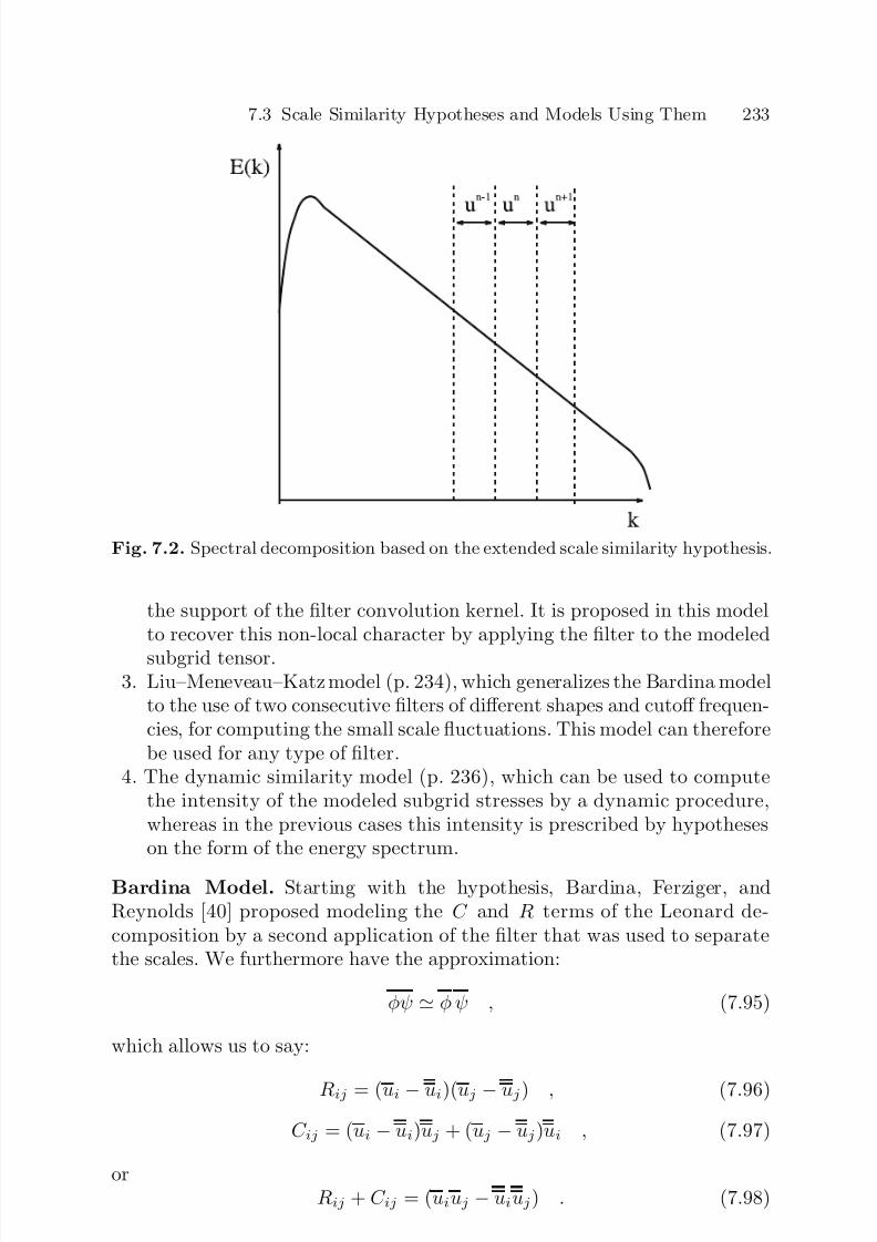
7/21/2019 Large Eddy Simulation for Incompressible Flows
http://slidepdf.com/reader/full/large-eddy-simulation-for-incompressible-flows 255/573
7.3 Scale Similarity Hypotheses and Models Using Them 233
Fig. 7.2. Spectral decomposition based on the extended scale similarity hypothesis.
the support of the filter convolution kernel. It is proposed in this modelto recover this non-local character by applying the filter to the modeled
subgrid tensor.3. Liu–Meneveau–Katz model (p. 234), which generalizes the Bardina model
to the use of two consecutive filters of different shapes and cutoff frequen-cies, for computing the small scale fluctuations. This model can thereforebe used for any type of filter.
4. The dynamic similarity model (p. 236), which can be used to computethe intensity of the modeled subgrid stresses by a dynamic procedure,whereas in the previous cases this intensity is prescribed by hypotheseson the form of the energy spectrum.
Bardina Model. Starting with the hypothesis, Bardina, Ferziger, andReynolds [40] proposed modeling the C and R terms of the Leonard de-composition by a second application of the filter that was used to separatethe scales. We furthermore have the approximation:
φψ φ ψ , (7.95)
which allows us to say:
Rij = (ui − ui)(uj − uj) , (7.96)
C ij = (ui − ui)uj + (uj − uj)ui , (7.97)
orRij + C ij = (uiuj − uiuj) . (7.98)

7/21/2019 Large Eddy Simulation for Incompressible Flows
http://slidepdf.com/reader/full/large-eddy-simulation-for-incompressible-flows 256/573
234 7. Structural Modeling
Adding Leonard’s term, which is computed directly from the resolvedscales, we get:
τ ij = Lij + Rij + C ij = (uiuj − uiuj) . (7.99)
This can be re-written in another using the generalized central momentsproposed by Germano [244]:
τ ij = τ G([ui]G, [uj]G) ≡ Lij . (7.100)
The subgrid tensor is therefore approximated by the generalized central
moment of the filtered field defined like the tensor Lij in the Germano decom-position (see Sect. 3.3.2). Experience shows that this model is not effectivewhen the filter is a Reynolds operator, because the contribution thus com-puted then cancels out. Contrary to the subgrid viscosity models, this onedoes not induce an alignment of the proper axis system of the subgrid tensoron those of the strain rate tensor. Tests performed on databases generated bydirect numerical simulation have shown that this model leads to a very goodlevel of correlation with the true subgrid tensor, including when the flow isanisotropic [320].
Despite its very good level of correlation6, experience shows that thismodel is only slightly dissipative and that it underestimates the energy cas-cade. It does, on the other hand, include the backward cascade mechanism.
Filtered Bardina Model. The Bardina model (7.99) is local in space inthe sense that it appears as a product of local values. This local characteris in contradiction with the non-local nature of the subgrid tensor, so thateach component appears in the form of a convolution product. To remedythis problem, Horiuti [323] and Layton and his colleagues [429, 428] proposethe filtered Bardina model:
τ ij = (uiuj − uiuj) = Lij . (7.101)
With this additional filtering operation, we recover the non-local characterof the subgrid tensor.
Liu–Meneveau–Katz Model. The Bardina model uses a second appli-cation of the same filter, and therefore a single cutoff scale. This model isgeneralized to the case of two cutoff levels as [455]:
τ ij = C l(uiuj − uiuj) = C lLmij , (7.102)
where the tensor Lmij is now defined by two different levels of filtering. The test
filter cutoff length designated by the tilde is larger than that of the first level.
6 The correlation coefficient at the scalar level is generally higher than 0.8.

7/21/2019 Large Eddy Simulation for Incompressible Flows
http://slidepdf.com/reader/full/large-eddy-simulation-for-incompressible-flows 257/573
7.3 Scale Similarity Hypotheses and Models Using Them 235
The constant C l can be evaluated theoretically to ensure that the averagevalue of the modeled generalized subgrid kinetic energy is equal to its exactcounterpart [148]. This leads to the relation:
C l = ukuk − ukuk ukuk − ukuk . (7.103)
Let F (k) and G(k) be transfer functions associated with the grid filterand test filter, respectively, and let E (k) be the energy spectrum of the exactsolution. Relation (7.103) can then be re-written as:
C l = ∞
0 (1
− F 2(k))E (k)dk ∞0 (1 − G2(k)) F 2(k)E (k)dk . (7.104)
Evaluations made using experimental data come to C l 1 [570, 455]7.Shah and Ferziger [668] propose extending this model to the case of non-symmetric filters.
To control the amplitude of the backward cascade induced by the model,especially near solid walls, Liu et al. [455] propose the modified form:
τ ij = C lf (I LS)Lmij , (7.105)
where the dimensionless invariant I LS, defined as
I LS = Lm
lkS lk LmlkLm
lk
S lkS lk
(7.106)
measures the alignment of the proper axes of the tensors Lm and S . As thekinetic energy dissipated by the subgrid model is expressed
ε =
−τ ijS ij , (7.107)
we get, using model (7.105):
ε = −C lf (I LS)I LS . (7.108)
The backward energy cascade is modulated by controlling the sign andamplitude of the product f (I LS)I LS. The authors considered a number of choices. The first is:
f (I LS) = 1 if I LS ≥ 0
0 otherwise
. (7.109)
This solution makes it possible to cancel out the representation of thebackward cascade completely by forcing the model to be strictly dissipative.
7 The initial value of 0.45 ± 0.15 given in [455] does not take the backward cascadeinto account.
7/21/2019 Large Eddy Simulation for Incompressible Flows
http://slidepdf.com/reader/full/large-eddy-simulation-for-incompressible-flows 258/573
236 7. Structural Modeling
One drawback to this is that the function f is discontinuous, which cangenerate numerical problems. A second solution that is continuous consistsin taking:
f (I LS) = I LS if I LS ≥ 0
0 otherwise . (7.110)
One last positive, continuous, upper-bounded solution is of the form:
f (I LS) =
(1 − exp(−γI 2LS)) if I LS ≥ 0
0 otherwise , (7.111)
in which γ = 10.
Dynamic Similarity Model. A dynamic version of the Liu–Meneveau–Katz model (7.102) was also proposed [455] for which the constant C l will nolonger be set arbitrarily. To compute this model, we introduce a third levelof filtering identified by .. The Q analogous to tensor Lm for this new levelof filtering is expressed:
Qij = (ui
uj −
ui uj) . (7.112)
The Germano–Lilly dynamic procedure, based here on the difference:
M ij = f (I QS)Qij − f (I LS)Lmij , (7.113)
where
I QS = Qmn
S mn
|Q| |S |, (7.114)
yields:
C l = LmlkM lk
M pqM pq. (7.115)
7.3.3 A Bridge Between Scale Similarity and ApproximateDeconvolution Models. Generalized Similarity Models
The Bardina model can be interpreted as a particular case of the approximatesoft deconvolution based models described in Sect. 7.2.
Using the second order differential approximation
φ = φ + α(2)
2
∂ 2φ
∂x2 , (7.116)
the Bardina model (7.99) is strictly equivalent to the second order gradientmodel given by relations (7.18) and (7.19).
7/21/2019 Large Eddy Simulation for Incompressible Flows
http://slidepdf.com/reader/full/large-eddy-simulation-for-incompressible-flows 259/573
7.4 Mixed Modeling 237
It can also be derived using the Van Cittert deconvolution procedure:a zeroth-order truncation in (7.7) is used to recover relation (7.95), whilea first-order expansion is employed to derive (7.96).
The Bardina model then appears as a low-order formal expansion modelfor the subgrid tensor. Generalized scale similarity models can then be de-fined using higher-order truncations for the formal expansion [254]. They areformulated as
τ ij = (G−1l ui)(G−1
l uj) − (G−1l u)i − (G−1
l u)j , (7.117)
where G−1l designates the approximate soft deconvolution operator, defined
in Sect. 7.2.1.The same key idea can be extended to close the Navier–Stokes on a trun-cated wavelet basis: this was achieved by Hoffman for several simplified sys-tems [315, 311, 309, 308].
7.4 Mixed Modeling
7.4.1 Motivations
The structural models based on the scale similarity idea and the soft de-convolution models/techniques on the one hand, and the functional modelson the other hand, each have their advantages and disadvantages that makethem seem complementary:
– The functional models, generally, correctly take into account the level of the energy transfers between the resolved scales and the subgrid modes.However, their prediction of the subgrid tensor structure, i.e. its eigenvec-tors, is very poor.
– The models based on the scale-similarity hypothesis or an approximate de-convolution procedure generally predict well the structure of the subgridtensor better (and then are able to capture anisotropic effects and dise-quilibrium), but are less efficient for dealing with the level of the energytransfers. It is also observed that these models yield a poor prediction of the subgrid vorticity production [491], a fact coherent with their under-dissipative character.
Dubois et al [202] also observed that these two parts yield different correla-
tions with reference data. Tests have shown that mixed models are able tocapture disequilibrium and anisotropy effects [8, 454, 504, 506, 594, 12].Shao et al. [670] propose a splitting of the kinetic energy transfer across
the cutoff that enlights the role of each one of these two model classes. Theseauthors combine the classical large-eddy simulation convolution filter to the

7/21/2019 Large Eddy Simulation for Incompressible Flows
http://slidepdf.com/reader/full/large-eddy-simulation-for-incompressible-flows 260/573
238 7. Structural Modeling
ensemble average, yielding the following decompositions:
u =
u
+ ue (7.118)
= u + u (7.119)
= u + u + ue + u . (7.120)
Using this hybrid decomposition, the subgrid tensor splits into
τ ij = τ rapidij + τ slow
ij , (7.121)
withτ slowij = uei u
ej
−ueiuej , (7.122)
τ rapidij = uiuj − uiuj + uei uj − ueiuj
+uej ui − uejui . (7.123)
These two parts can be analysed as follows:
– The rapid part explicitly depends on the mean flow. This contributionarises only if the convolution filter is applied in directions where the meanflow gradients are non-zero. It is referred to as rapid because the time scaleof its response to variations of the mean flow is small. Numerical exper-iments show that this part plays an important role when the turbulenceis in a desiquilibrium state when: (i) production of kinetic energy is muchlarger than dissipation or (ii) the filter length is of the same order as theintegral scale of turbulence. Subgrid stresses anisotropy is observed to bedue to the interaction of this rapid part and the mean shear. Numericalsimulations have shown that the rapid part escapes the functional mod-eling, but scale-similarity models and soft deconvolution models succeedin representing anisotropic energy transfer (both forward and backward
cascades) associated to the rapid part.– The slow part is always present in large-eddy simulation, because it does
not depend on the mean flow gradients. It corresponds to the subgrid tensoranalyzed through the previously described canonical analysis. It is referredto as slow because its relaxation time is long with respect to rapid part.Numerical tests show that subgrid viscosity model correctly capture theassociated kinetic energy transfer.
One simple idea for generating subgrid models possessing good qualities
on both the structural and energy levels is to combine a functional witha structural model, making what is called mixed models. This is generallydone by combining a subgrid viscosity model for representing the energycascade mechanism with a scale similarity. The stochastic backward cascademodels are usually not included because the structural models are capable of including this phenomenon.
7/21/2019 Large Eddy Simulation for Incompressible Flows
http://slidepdf.com/reader/full/large-eddy-simulation-for-incompressible-flows 261/573
7.4 Mixed Modeling 239
The resulting form is
τ ij − 1
3 τ kkδ ij = −2ν sgsS ij + (Lij − 1
3 Lkkδ ij) , (7.124)
where ν sgs is the subgrid viscosity (evaluated using one of the previouslydescribed model), and Lij the evaluation obtained using one of the structuralmodel8.
Another argument for using a mixed model originates from the splittingof the full deconvolution model as the sum of the soft deconvolution modeland the hard deconvolution model (see Sect. 7.2.1): the scale-similarity mod-els are formally equivalent to truncated Taylor-series-expansion-based soft
deconvolution models, and thus are not able to account for interactions be-tween resolved scales and scales smaller than the mesh size on which theequations are solved. Consequently, they must be supplemented by anothermodel, which will play the role of the secondary regularization within theframework of the deconvolution approach.
Examples of such models are described in the following.
7.4.2 Examples of Mixed Models
We present several examples of mixed models here:1. The Smagorinsky–Bardina model (p. 240), for which the respective
weights of each of the contributions are preset. This model is limitedby the hypotheses underlying each of the two parts constituting it: thesubgrid viscosity is still based on arguments of the infinite inertial rangetype. Experience shows, though, that combining the two models reducesthe importance of the constraints associated with these underlying hy-potheses, which improves the results.
2. A one-parameter mixed model whose subgrid viscosity is computed by
a dynamic procedure of the Germano–Lilly type (p. 240). With this pro-cedure, the respective weights of the structural and functional parts of the model can be modified, so that the subgrid viscosity model is nowcomputed as a complement to the scale similarity model, which allowsa better control of the dissipation induced. It can be said, though, thatthis procedure innately prefers the structural part.
3. The general form of N -parameter dynamic mixed model, as derived bySagaut et al. (p. 241). This procedure is an extension of the previous one:the weights of the different parts of the model are dynamically computed,
resulting in a possibly better approximation of the true subgrid stresses.The case of two-parameter dynamic mixed model is emphasized.
8 Only scale-similarity models or approximate deconvolution models are used inpractice to derive mixed models, because they are very easy to implement.

7/21/2019 Large Eddy Simulation for Incompressible Flows
http://slidepdf.com/reader/full/large-eddy-simulation-for-incompressible-flows 262/573
240 7. Structural Modeling
Other mixed models have already been presented within the frameworkof the deconvolution approach (see Sect. 7.2.1, p. 220), which will not berepeated in the present section. Application of the results dealing with thedynamic evaluation of the constants presented below to the Taylor seriesexpansion based deconvolution models is straightforward.
Mixed Smagorinsky–Bardina Model. The first example is proposed byBardina et al. [40] in the form of a linear combination of the Smagorinskymodel (5.90) and the scale similarity model (7.99). The subgrid tensor devi-ator is then written:
τ ij −
1
3
τ kkδ ij = 1
2 −2ν sgsS ij +
Lij
− 1
3Lkkδ ij , (7.125)
in which
Lij =
ui uj − ui uj
, (7.126)
and
ν sgs = C s∆2|S | . (7.127)
Variants are obtained either by changing the subgrid viscosity modelused or by replacing the tensor L with the tensor Lm (7.105) or the ten-sor L (7.101).
One-Parameter Mixed Dynamic Model. A mixed dynamic model wasproposed by Zang, Street, and Koseff [799]. This is based initially on theBardina model coupled with the Smagorinsky model, but the latter can bereplaced by any other subgrid viscosity model. The subgrid viscosity modelconstant is computed by a dynamic procedure. The subgrid tensors corre-sponding to the two filtering levels are modeled by a mixed model:
τ ij − 1
3τ kkδ ij = −2ν sgsS ij + Lm
ij − 1
3Lmkkδ ij , (7.128)
T ij − 1
3T kkδ ij = −2ν sgs
S ij + Qij − 1
3Qkkδ ij , (7.129)
in which
Qij = uiuj − uiuj , (7.130)
and
ν sgs = C d∆|S | . (7.131)

7/21/2019 Large Eddy Simulation for Incompressible Flows
http://slidepdf.com/reader/full/large-eddy-simulation-for-incompressible-flows 263/573
7.4 Mixed Modeling 241
The residual E ij is now of the form:
E ij =L
m
ij − Hij
− −2C d∆2
mij + δ ijP kk , (7.132)
in whichHij = uiuj − uiuj , (7.133)
Lmij = uiuj − uiuj , (7.134)
mij =
∆∆
2
|S |S ij − |S |S ij , (7.135)
and where P kk represents the trace of the subgrid tensor. The Germano–Lillydynamic procedure leads to:
C d =(Lmij − Hij)mij
mijmij. (7.136)
In simulations performed with this model, the authors observed a reduc-tion in the value of the dynamic constant with respect to that predicted bythe usual dynamic model (i.e. based on the Smagorinsky model alone). Thiscan be explained by the fact that the difference between the Lm and H termsappears in the numerator of the fraction (7.136) and that this difference issmall because these terms are very similar. This shows that the subgrid vis-
cosity model serves only to model a residual part of the full subgrid tensorand not its entirety, as in the usual dynamic model.
Vreman et al. [747] propose a variant of this model. For the sake of math-ematical consistency, by making the model for the tensor T ij dependent only
on the velocity field that corresponds to the same level of filtering, i.e. u,these authors propose the following alternate form for the tensor Qij :
Qij =
ui
uj −
ui
uj . (7.137)
N-Parameter Dynamic Mixed Model.
General Formulation and Formal Resolution. A general form of multiparam-eter dynamic model was derived by Sagaut et al. [630]. Considering a formalN -part parametrization of the subgrid tensor, each term being associated toa real constant C l, k = 1,..,N
τ ij =l=1,N
C lf lij(u, ∆) , (7.138)
where the functions f lij are the kernels of the different parts of the completemodel. The equivalent formulation obtained at the test filter level is
T ij =l=1,N
C lf lij(u, ∆) . (7.139)
7/21/2019 Large Eddy Simulation for Incompressible Flows
http://slidepdf.com/reader/full/large-eddy-simulation-for-incompressible-flows 264/573
242 7. Structural Modeling
Inserting (7.138) and (7.139) into the Germano identity (5.138), we getthe following definition of the residual E ij :
E ij = Lij − l=1,N
C lmlij , ml
ij = f lij(u, ∆) − f lij(u, ∆) . (7.140)
In order to obtain N linearly independent relations to compute the con-stants C l, a first solution is to operate the contraction of the residual (7.140)with N independent tensors Alij. The constants will then appear as the so-lutions of the following linear algebraic problem of rank N :
l=1,N
C lmlijA
kji = LijAkji , k = 1, N . (7.141)
It is worth noting that the N constants are coupled, resulting in a globalself-adaption of each constant. The particular case of the least-square mini-mization is recovered by taking Akij = mk
ij, k = 1, N .In the case where some constants are not computed dynamically but are
arbitrarily set, the linear system (7.141) corresponds to a ill-posed problemcontaining more constraints than degrees of freedom. Assuming that the N
first constants are arbitrarily chosen, we recover a well-posed problem of rank
N − N
by replacing Lij with L
ij , where
Lij = Lij −
l=1,N
C lmlij . (7.142)
Two-Parameter Dynamic Models. Mixed models have also been proposed bySalvetti [640, 643] and Horiuti [324] with two dynamic constants (one forthe subgrid-viscosity part and one for the scale-similarity), corresponding tothe N = 2 case in the previous section. These models have the advantage of avoiding any a priori preference for the contribution of one or the other model
component. An extensive study of dynamic mixed model has been carried outby Sarghini et al. [646] for the plane channel case.
Numerical simulations show that two-paramater mixed models may yielddisappointing results, because of a too low dissipation level. This is due to thefact that the coupled dynamic procedure described in the previous sectiongives a heavy weigth to the scale-similarity part of the model, because its cor-relation coefficient with the exact subgrid tensor is much higher than the oneof the subgrid-viscosity model. This conclusion was confirmed by Andersonand Meneveau [12] in isotropic turbulence. These authors also observed a se-
rious lack of robustness in regard to the dynamic Smagorinsky model whenthe test filter cutoff exceeds the integral scale of turbulence: negative valuesof the dynamic constant are returned in this case. To relieve this problem,Morinishi [542, 543] proposes to uncouple the computation of the dynamicconstants. The modified algorithm for the dynamic procedure is:

7/21/2019 Large Eddy Simulation for Incompressible Flows
http://slidepdf.com/reader/full/large-eddy-simulation-for-incompressible-flows 265/573
7.5 Differential Subgrid Stress Models 243
1. Compute the constant associated to the subgrid-viscosity part of themodel using a classical dynamic procedure, without taking the scale sim-ilarity part into account. This corresponds to the N = 1 case in theprevious section. The resulting constant will ensure a correct level of dissipation.
2. Compute the constant associated to the scale-similarity part using a two-parameter dynamic procedure, but considering that the constant of thesubgrid-viscosity part is fixed. This corresponds to N = 2 and N = 1 inthe previous section.
7.5 Differential Subgrid Stress ModelsA natural way to find an expression for the subgrid stress tensor is to solvea prognostic equation for each component. This approach leads to the defini-tion of six additional equations, and thus a very significant increase in boththe model complexity and the computational cost. But the expected advan-tage is that such a model would a priori be able to account for a large classof physical mechanisms, yielding the definition of a very robust model. Threeproposal have been published by different research groups:
1. The pioneering model of Deardorff (p. 243).2. The model by Fureby et al. (p. 244), which is an improved version of the
Deardorff model with better theoretical properties, such as realizability.3. The models based of the use of transport equations for the velocity filtered
probability density function (p. 245), which do not rely on an explicitmodel for the triple correlations.
7.5.1 Deardorff Model
Another approach for obtaining a model for the subgrid tensor consists insolving an evolution equation for each of its components. This approach pro-posed by Deardorff [173] is analogous in form to two-point statistical mod-eling. Here, we adopt the case where the filter is a Reynolds operator. Thesubgrid tensor τ ij is thus reduced to the subgrid Reynolds tensor Rij . Wededuce the evolution equation of the subgrid tensor components from that of the subgrid modes (3.31)9:
∂τ ij
∂t
=
− ∂
∂xk(ukτ ij)
−τ ik
∂uj
∂xk −τ jk
∂ui
∂xk
9 This is done by applying the filter to the relation obtained by multiplying (3.31)by uj and taking the half-sum with the relation obtained by inverting the sub-scripts i and j.
7/21/2019 Large Eddy Simulation for Incompressible Flows
http://slidepdf.com/reader/full/large-eddy-simulation-for-incompressible-flows 266/573
244 7. Structural Modeling
− ∂
∂xkuiu
juk + p
∂ui∂xj
+∂uj∂xi
− ∂
∂xjui p
− ∂ ∂xi
uj p − 2ν ∂ui
∂xk∂uj∂xk
. (7.143)
The various terms in this equation have to be modeled. The models Dear-dorff proposes are:
– For the pressure–strain correlation term:
p∂ui
∂xj+
∂uj
∂xi =
−C m
q 2sgs
∆ τ ij −
2
3q 2sgsδ ij+
2
5q 2sgsS ij , (7.144)
where C m is a constant, q 2sgs the subgrid kinetic energy, and S ij the strainrate tensor of the resolved field.
– For the dissipation term:
ν ∂ui∂xk
∂uj∂xk
= δ ijC e(q 2sgs)3/2
∆, (7.145)
where C e is a constant.
– For the triple correlations:
uiujuk = −C 3m∆
q 2sgs
∂
∂xiτ jk +
∂
∂xjτ ik +
∂
∂xkτ ij
. (7.146)
The pressure–velocity correlation terms pui are neglected. The values of the constants are determined in the case of isotropic homogeneous turbulence:
C m = 4.13, C e = 0.70, C 3m = 0.2 . (7.147)
Lastly, the subgrid kinetic energy is determined using evolution equa-tion (5.119).
7.5.2 Fureby Differential Subgrid Stress Model
An alternate form of the differential stress model is proposed by Fureby etal. [232], which has better symmetry preservation properties than the originalDeardorff model. The triple correlation term is approaximated as
−uiuju
k = cq q 2sgs∆
ν sgs
∂τ ij∂xk
, (7.148)
with cq = 0.07. Other terms are kept unchanged. Each term in the closedsubgrid stress equations is now frame indifferent. The set of closed equations

7/21/2019 Large Eddy Simulation for Incompressible Flows
http://slidepdf.com/reader/full/large-eddy-simulation-for-incompressible-flows 267/573
7.5 Differential Subgrid Stress Models 245
is realizable, and has the same transformation properties as the exact Navier–Stokes equations under a change of frame.
An alternate form of the subgrid viscosity in (7.148) which allows therepresentation of backscatter is also defined by Fureby:
ν sgs = − τ ijS ij
S ijS ij. (7.149)
7.5.3 Velocity-Filtered-Density-Function-Based SubgridStress Models
A methodology referred to as the Velocity Filtered Density Function to closethe filtered Navier–Stokes equations is proposed by Gicquel et al. [264] on thegrounds of the previous works by Pope and Givi. The subgrid scale stressesare reconstructed by considering the joint probability function of all of thecomponents of the velocity vector. To this end, an exact evolution equation isderived for the velocity filtered density function in which unclosed terms aremodeled. Two implementations have been proposed: a first one consists indiscretizing transport equations for the subgrid stresses associated to the ve-locity filtered density function (this is the one emphasized below); the second
one consists in solving it via a Lagrangian Monte Carlo scheme, which leadsto the definition of an equivalent stochastic system. This last form shouldbe classified as a structural model based on a stochastic reconstruction of subgrid scales, and will be mentioned in Sect. 7.7.
Definitions. The first step consists in defining the velocity filtered densityfunction P L
P L(v; x, t) =
+∞
−∞
ρ[v, u(x, t)]G(x − x)dx , (7.150)
where G is the convolution filter kernel and ρ[v, u(x, t)] is the fine-graineddensity
ρ[v, u(x, t)] = δ (v − u(x, t)) . (7.151)
It is observed that P L has all the properties of the probability densityfunction when the filter kernel is positive. The conditional filtered value of a dummy variable φ(x, t) is therefore defined as
φ(x, t)|u(x, t) = vL = φ|vL +∞−∞
φ(x, t)ρ[v, u(x, t)]G(x − x)dx
P L(v; x, t) .
(7.152)where α|β L denotes the filtered value of α conditioned on β .
7/21/2019 Large Eddy Simulation for Incompressible Flows
http://slidepdf.com/reader/full/large-eddy-simulation-for-incompressible-flows 268/573
246 7. Structural Modeling
First Model. The starting point of the procedure is to write an expressionfor the time-derivative of P L. Such an expression is found by applying thetime-derivative operator to Eq. (7.150), yielding
∂P L(v; x, t)
∂t =
+∞
−∞
∂ui(x, t)
∂t
∂ρ[v, u(x, t)]
∂viG(x − x)dx
= − ∂
∂vi
∂ui∂t
v
L
P L(v; x, t)
(7.153)
The next step consists in eliminating the velocity time derivative usingthe momentum equation, leading to
∂P L∂t
+ uk∂P L∂xk
= − ∂
∂xk[(vk − uk) P L] +
∂p
∂xi
∂P L∂vi
− 2ν ∂S ik∂xk
∂P L∂vi
+ ∂
∂vi
∂p
∂xi
v
L
− ∂p
∂xi
P L
− 2ν
∂
∂vi
∂S ik∂xi
v
L
− ∂S ik∂xi
P L
, (7.154)
where the relation
φ ≡ G φ =
+∞
−∞
φ|vLP L(v; x, t)dv , (7.155)
was used. The last two terms in the right hand side of (7.154) are unclosedterms which require the definition of ad hoc subgrid models. The first termin the right hand side is related to the subgrid advection and is closed. Thesum of the two unknown terms is modeled as follows
∂ ∂vi
∂p∂xi
vL
− ∂p∂xi
P L− 2ν ∂ ∂vi
∂S ik∂xi
vL
− ∂S ik∂xi
P L − ∂
∂vi[Gij(vj − ui)P L]
1
2C 0ε
∂ 2P L∂vi∂vi
,(7.156)
with
Gij = −ω
1
2 +
3
4C 0
δ ij , (7.157)
with C 0 = 2.1 and where the subgrid dissipation rate ε and the subgridmixing frequency ω are evaluated as
ε =
q 2sgs
3/2
∆, ω =
ε
q 2sgs
. (7.158)
7/21/2019 Large Eddy Simulation for Incompressible Flows
http://slidepdf.com/reader/full/large-eddy-simulation-for-incompressible-flows 269/573
7.5 Differential Subgrid Stress Models 247
The subgrid kinetic energy q 2sgs is taken equal to half the trace of thesubgrid stress tensor. This closure is equivalent the the one proposed byRotta for the Reynolds-averaged Navier–Stokes equations.
The final stage consists in writing the corresponding equations for thesubgrid stresses, which are defined here using the generalized central mo-ment framework of Germano (Sect. 3.3.2), i.e. τ ij = τ G(ui, uj). Evolutionequations consistant with the previous closed form of the velocity filtereddensity function are
∂τ ij∂t
+ ∂
∂xk(ukτ ij) = −∂τ ijk
∂xk+ Gikτ jk + Gjkτ ik
−τ ik
∂uj
∂xk − τ jk
∂ui
∂xk + C 0εδ ij . (7.159)
The last unknown term is the third-order generalized central momentτ ijk = τ G(ui, uj , uk). Its value are taken from the Lagrangian Monte Carlosolver used to generate a prognostic stochastic velocity field whose pdf P Lsatisfies equation (7.154). Details of the numerical implementation can befound in Ref. [264] and will not be reproduced here.
Second Model. An alternative form for relation (7.154) is
∂P L∂t
+ uk ∂P L∂xk
= − ∂ ∂xk
[(vk − uk) P L] + ∂p∂xi
∂P L∂vi
+ ∂
∂vi
∂p
∂xi
v
L
− ∂p
∂xi
P L
+ ν
∂ 2P L∂xk∂xk
− ∂ 2
∂vi∂vi
ν
∂ui∂xk
∂uj∂xk
v
L
P L
. (7.160)
Using the same procedure as in the previous case, the following closedform is obtained
∂P L∂t
+ uk∂P L∂xk
= − ∂
∂xk[(vk − uk) P L] +
∂p
∂xi
∂P L∂vi
+ν ∂ui∂xk
∂uj∂xk
∂ 2P L∂vi∂vj
+ 2ν ∂ui∂xk
∂ 2P L∂vi∂vk
− ∂
∂vi(Gij(vj − uj)P L) +
1
2C 0ε
∂ 2P L∂vi∂vj
. (7.161)
The consistent subgrid stress equations are now
∂τ ij∂t
+ ∂
∂xk(ukτ ij) = −∂τ ijk
∂xk+ Gikτ jk + Gjkτ ik
+ν ∂ 2τ ij∂xk∂xk
− τ ik∂uj∂xk
− τ jk∂ui∂xk
+ C 0εδ ij . (7.162)
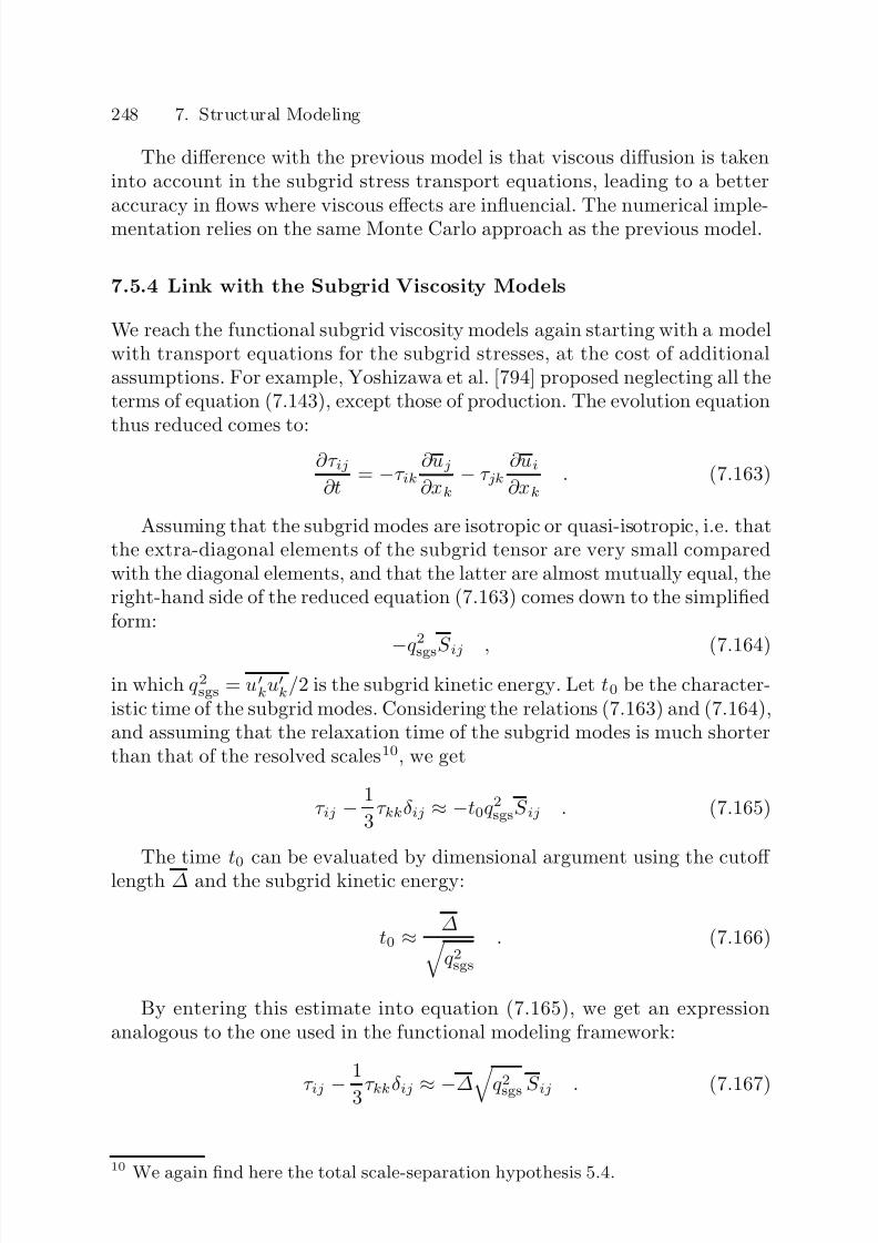
7/21/2019 Large Eddy Simulation for Incompressible Flows
http://slidepdf.com/reader/full/large-eddy-simulation-for-incompressible-flows 270/573
248 7. Structural Modeling
The difference with the previous model is that viscous diffusion is takeninto account in the subgrid stress transport equations, leading to a betteraccuracy in flows where viscous effects are influencial. The numerical imple-mentation relies on the same Monte Carlo approach as the previous model.
7.5.4 Link with the Subgrid Viscosity Models
We reach the functional subgrid viscosity models again starting with a modelwith transport equations for the subgrid stresses, at the cost of additionalassumptions. For example, Yoshizawa et al. [794] proposed neglecting all theterms of equation (7.143), except those of production. The evolution equationthus reduced comes to:
∂τ ij∂t
= −τ ik∂uj∂xk
− τ jk∂ui∂xk
. (7.163)
Assuming that the subgrid modes are isotropic or quasi-isotropic, i.e. thatthe extra-diagonal elements of the subgrid tensor are very small comparedwith the diagonal elements, and that the latter are almost mutually equal, theright-hand side of the reduced equation (7.163) comes down to the simplifiedform:
−q
2
sgsS ij , (7.164)in which q 2sgs = ukuk/2 is the subgrid kinetic energy. Let t0 be the character-istic time of the subgrid modes. Considering the relations (7.163) and (7.164),and assuming that the relaxation time of the subgrid modes is much shorterthan that of the resolved scales10, we get
τ ij − 1
3τ kkδ ij ≈ −t0q 2sgsS ij . (7.165)
The time t0 can be evaluated by dimensional argument using the cutoff length ∆ and the subgrid kinetic energy:
t0 ≈ ∆ q 2sgs
. (7.166)
By entering this estimate into equation (7.165), we get an expressionanalogous to the one used in the functional modeling framework:
τ ij − 1
3 τ kkδ ij ≈ −∆ q 2sgs S ij . (7.167)
10 We again find here the total scale-separation hypothesis 5.4.

7/21/2019 Large Eddy Simulation for Incompressible Flows
http://slidepdf.com/reader/full/large-eddy-simulation-for-incompressible-flows 271/573
7.6 Stretched-Vortex Subgrid Stress Models 249
7.6 Stretched-Vortex Subgrid Stress Models
7.6.1 General
Misra and Pullin [517, 608, 735], following on the works of Pullin andSaffman [609], proposed subgrid models using the assumption that the sub-grid modes can be represented by stretched vortices whose orientation isgoverned by the resolved scales.
Supposing that the subgrid modes can be linked to a random superimpo-sition of fields generated by axisymmetrical vortices, the subgrid tensor canbe written in the form:
τ ij = 2 ∞kcE (k)dkE piZ pqE qj , (7.168)
in which E (k) is the energy spectrum, E lm the rotation matrix used to switchfrom the vortex coordinate system to the reference system, Z ij the diagonaltensor whose main elements are (1/2, 1/2, 0) and E piZ pqE qj , the momentof the probability density function P (α, β ) of the Euler angles α and β givingthe orientation of the vortex axis with respect to the frame of reference. Thestatistical average performed on the Euler angles of a function f is definedas:
f (E ij) = 14π π
0
2π
0
f (E ij)P (α, β )sin(α)dαdβ . (7.169)
Two pieces of information are therefore needed to compute the subgridterm: the shape of the energy spectrum for the subgrid modes and the subgridstructure orientation distribution function. As the use of an evolution equa-tion for the probability density function yielded no satisfactory results, Misraand Pullin propose modeling this function as a product of Dirac functions ora linear combination of such products. These are of the general form:
P (α, β ) = 4πsin(α)
δ (α − θ)δ (β − φ) , (7.170)
where θ(x, t) and φ(x, t) determine the specific orientation considered. Defin-ing the two unit vectors e and ev:
e1 = sin(α)cos(β ), e2 = sin(α)sin(β ), e3 = cos(α), (7.171)
ev1 = sin(θ)cos(φ), ev2 = sin(θ)sin(φ), ev3 = cos(θ), (7.172)
the subgrid tensor can be re-written in the form:
τ ij =
δ ij − evi evj ∞kc
E (k)dk =
δ ij − evi evj
q 2sgs . (7.173)

7/21/2019 Large Eddy Simulation for Incompressible Flows
http://slidepdf.com/reader/full/large-eddy-simulation-for-incompressible-flows 272/573
250 7. Structural Modeling
The various models must thus specify the specific orientation directions of the subgrid structures. Three models are presented in the following. The sub-grid kinetic energy q 2
sgs can be computed in different ways (see Sect. 9.2.3),
for example by solving an additional evolution equation, or by using a dou-ble filtering technique. A local evaluation procedure in the physical spacebased on the second-order velocity structure function is proposed by Voeklet al. [735].
7.6.2 S3/S2 Alignment Model
A first hypothesis is to assume that the subgrid structures are oriented alongthe eigenvectors of the resolved strain rate tensor S ij that corresponds to
its two largest eigenvalues. This is equivalent to assuming that they respondinstantaneously to the forcing of the large scales. Using es2 and es3 to denotethese two vectors, and λ2 and λ3 ≥ λ2 the associated eigenvalues, we get
τ ij = q 2sgs
λ
δ ij − es3i es3j
+ (1 − λ)
δ ij − es2
i es2j
, (7.174)
where the weighting coefficient is taken proportional to the norms of theeigenvalues:
λ = λ3
λ3 +
|λ2
|
. (7.175)
7.6.3 S3/ω Alignment Model
The second model is derived on the assumption that the subgrid structuresare oriented along the third eigenvector of the tensor S ij , denoted es3 asbefore, and the vorticity vector of the resolved field. The unit vector it carriesis denoted eω and is computed as:
eω = ∇ × u
|∇ ×u
|
. (7.176)
The subgrid tensor is evaluated as:
τ ij = q 2sgs
λ
δ ij − es3i es3j
+ (1 − λ)
δ ij − eωi e
ωj
. (7.177)
The weighting parameter λ is chosen arbitrarily. The authors performedtests considering the three values 0, 0.5, and 1.
7.6.4 Kinematic Model
Starting with the kinematics of a vortex filament entrained by a fixed velocity
field, Misra and Pullin propose a third model, for which the vector ev is ob-tained by solving an evolution equation. The equation for the ith componentof this vector is:
∂evi∂t
= evj∂ui∂xj
− evi evkevj∂uk∂xj
. (7.178)
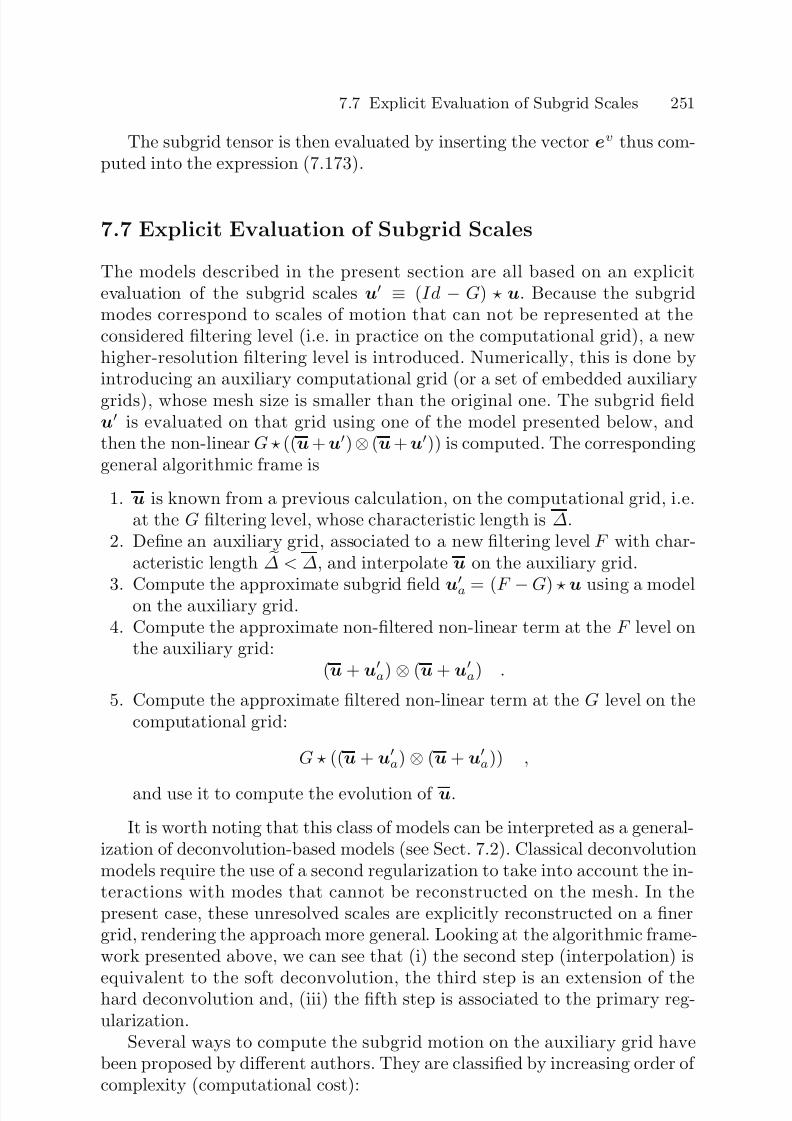
7/21/2019 Large Eddy Simulation for Incompressible Flows
http://slidepdf.com/reader/full/large-eddy-simulation-for-incompressible-flows 273/573
7.7 Explicit Evaluation of Subgrid Scales 251
The subgrid tensor is then evaluated by inserting the vector ev thus com-puted into the expression (7.173).
7.7 Explicit Evaluation of Subgrid Scales
The models described in the present section are all based on an explicitevaluation of the subgrid scales u ≡ (Id − G) u. Because the subgridmodes correspond to scales of motion that can not be represented at theconsidered filtering level (i.e. in practice on the computational grid), a newhigher-resolution filtering level is introduced. Numerically, this is done byintroducing an auxiliary computational grid (or a set of embedded auxiliarygrids), whose mesh size is smaller than the original one. The subgrid fieldu is evaluated on that grid using one of the model presented below, andthen the non-linear G ((u + u) ⊗ (u + u)) is computed. The correspondinggeneral algorithmic frame is
1. u is known from a previous calculation, on the computational grid, i.e.at the G filtering level, whose characteristic length is ∆.
2. Define an auxiliary grid, associated to a new filtering level F with char-acteristic length
∆ < ∆, and interpolate u on the auxiliary grid.
3. Compute the approximate subgrid field u
a = (F − G) u using a modelon the auxiliary grid.4. Compute the approximate non-filtered non-linear term at the F level on
the auxiliary grid:(u + u
a) ⊗ (u + ua) .
5. Compute the approximate filtered non-linear term at the G level on thecomputational grid:
G ((u + ua) ⊗ (u + u
a)) ,
and use it to compute the evolution of u.
It is worth noting that this class of models can be interpreted as a general-ization of deconvolution-based models (see Sect. 7.2). Classical deconvolutionmodels require the use of a second regularization to take into account the in-teractions with modes that cannot be reconstructed on the mesh. In thepresent case, these unresolved scales are explicitly reconstructed on a finergrid, rendering the approach more general. Looking at the algorithmic frame-work presented above, we can see that (i) the second step (interpolation) is
equivalent to the soft deconvolution, the third step is an extension of thehard deconvolution and, (iii) the fifth step is associated to the primary reg-ularization.
Several ways to compute the subgrid motion on the auxiliary grid havebeen proposed by different authors. They are classified by increasing order of complexity (computational cost):
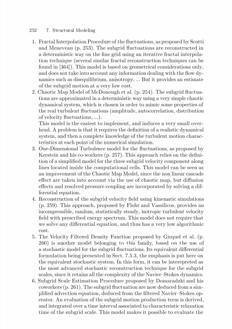
7/21/2019 Large Eddy Simulation for Incompressible Flows
http://slidepdf.com/reader/full/large-eddy-simulation-for-incompressible-flows 274/573
252 7. Structural Modeling
1. Fractal Interpolation Procedure of the fluctuations, as proposed by Scottiand Meneveau (p. 253). The subgrid fluctuations are reconstructed ina deterministic way on the fine grid using an iterative fractal interpola-tion technique (several similar fractal reconstruction techniques can befound in [364]). This model is based on geometrical considerations only,and does not take into account any information dealing with the flow dy-namics such as disequilibrium, anisotropy, ... But it provides an estimateof the subgrid motion at a very low cost.
2. Chaotic Map Model of McDonough et al. (p. 254). The subgrid fluctua-tions are approximated in a deterministic way using a very simple chaoticdynamical system, which is chosen in order to mimic some properties of the real turbulent fluctuations (amplitude, autocorrelation, distribution
of velocity fluctuations, ...).This model is the easiest to implement, and induces a very small over-head. A problem is that it requires the definition of a realistic dynamicalsystem, and then a complete knowledge of the turbulent motion charac-teristics at each point of the numerical simulation.
3. One-Dimensional Turbulence model for the fluctuations, as proposed byKerstein and his co-workers (p. 257). This approach relies on the defini-tion of a simplified model for the three subgrid velocity component alonglines located inside the computational cells. This model can be seen as
an improvement of the Chaotic Map Model, since the non linear cascadeeffect are taken into account via the use of chaotic map, but diffusioneffects and resolved pressure coupling are incorporated by solving a dif-ferential equation.
4. Reconstruction of the subgrid velocity field using kinematic simulations(p. 259). This approach, proposed by Flohr and Vassilicos, provides anincompressible, random, statistically steady, isotropic turbulent velocityfield with prescribed energy spectrum. This model does not require thatwe solve any differential equation, and thus has a very low algorithmic
cost.5. The Velocity Filtered Density Function proposed by Gicquel et al. (p.
260) is another model belonging to this family, based on the use of a stochastic model for the subgrid fluctuations. Its equivalent differentialformulation being presented in Sect. 7.5.3, the emphasis is put here onthe equivalent stochastic system. In this form, it can be interepreted asthe most advanced stochastic reconstruction technique for the subgridscales, since it retains all the complexity of the Navier–Stokes dynamics.
6. Subgrid Scale Estimation Procedure proposed by Domaradzki and his
coworkers (p. 261). The subgrid fluctuation are now deduced from a sim-plified advection equation, deduced from the filtered Navier–Stokes op-erator. An evaluation of the subgrid motion production term is derived,and integrated over a time interval associated to characteristic relaxationtime of the subgrid scale. This model makes it possible to evaluate the

7/21/2019 Large Eddy Simulation for Incompressible Flows
http://slidepdf.com/reader/full/large-eddy-simulation-for-incompressible-flows 275/573
7.7 Explicit Evaluation of Subgrid Scales 253
subgrid motion at a very low computational cost, but requires the com-putation of an approximate inverse filter.
7. Multilevel Simulations (p. 263), which are based on the use of the exactNavier–Stokes equations on a set of embedded computational grids. Thereduction of the computational effort with respect to the Direct Numer-ical Simulation is obtained by freezing (quasi-static approximation) thehigh-frequencies represented on fine grids for some time interval, leadingto the definition of a cyclic strategy. These methods can be interpretedas a time-consistent extension of the classical multigrid procedures forsteady computations. They correspond to the maximal computationaleffort, but also to the most realistic approach.
7.7.1 Fractal Interpolation Procedure
Scotti and Meneveau [661, 662] propose to reconstruct the subgrid velocityfield using two informations: (i) the resolved velocity field, which is known onthe coarsest grid, and (ii) the fractality of the velocity field. The fluctuationsare evaluated by interpolating the resolved coarse-grid velocity field on thefine grid using a fractal interpolation technique.
We first describe this interpolation technique in the monodimensionalcase. It is based on an iterative mapping procedure. The fluctuating field
ua is reconstructed within each interval of the coarse grid by introducing
a local coordinate ξ ∈ [0, 1]. Let us consider the interval [xi−1, xi+1], wherei − 1 and i + 1 are related to the grid index on the coarse grid. We have ξ =(x − xi−1)/2∆. The proposed map kernel W for a function φ to interpolatedon the considered interval is:
W [φ](ξ ) =
di,1φ(2ξ ) + q i,1(2ξ ) if ξ ∈ [0, 1/2]di,2φ(2ξ ) + q i,2(2ξ ) if ξ ∈]1/2, 1]
, (7.179)
where q i,j are polynomials and di,j are stretching parameters. The authorspropose to use the following linear polynomials:
q i,1(ξ ) = (φ(xi) − φ(xi−1) − di,1(φ(xi+1) − φ(xi−1))ξ
+φ(xi−1)(1 − di,1) , (7.180)
q i,2(ξ ) = (φ(xi+1) − φ(xi) − di,2(φ(xi+1) − φ(xi−1))ξ
−φ(xi−1)di,2 . (7.181)
The fluctuation is defined as
ua = lim
n→∞W n[u] = W W ... W [u]
n times
. (7.182)

7/21/2019 Large Eddy Simulation for Incompressible Flows
http://slidepdf.com/reader/full/large-eddy-simulation-for-incompressible-flows 276/573
254 7. Structural Modeling
The stretching parameters are such that the Hausdorff dimension D of the synthetic signal is equal to
D = 1 + log(|di,1|+|di,2|)
log(2) if 1 < |di,1| + |di,2| < 2
1 if |di,1| + |di,2| ≤ 1. (7.183)
In order to conserve then mean value of the signal over the consideredinterval, we have di,1 = −di,2 = d. For three-dimensional isotropic turbulence,we have D = 5/3, yielding d = ∓21/3.
This procedure theoretically requires an infinite number of iterations tobuild the fluctuating field. In practice, a finite number of iterations is used.The statistical convergence rate of process being exponential, it still remains
a good approximation. A limited number of iterations can also be seen asa way to account for viscous effects.
The extension to the multidimensional case is straightforward, each di-rection of space being treated sequentially.
This procedure also makes it possible to compute analytically the sub-grid tensor. The resulting model will not be presented here (see [662] fora complete description).
7.7.2 Chaotic Map Model
McDonough and his coworkers [552, 338, 469] propose an estimation proce-dure based on the definition of a chaotic dynamical system. The resultingmodel generates a contravariant subgrid-scale velocity field, represented atdiscrete time intervals on the computational grid:
ua = Auζ V , (7.184)
where A is an amplitude coefficient evaluated from canonical analysis, ζ ananisotropy correction vector consisting mainly of first-order structure func-
tion of high-pass filtered resolved scales, and V is a vector of chaotic algebraicmaps. It is important noting that the two vectors are multiplied using a vec-tor Hadamard product, defined for two vectors and a unit vector i accordingto:
(ζ V ) · i ≡ (ζ · i)(V · i) . (7.185)
The amplitude factor is chosen such that the kinetic energy of the syn-thetic subgrid motion is equal to the energy contained in all the scales notresolved by the simulation. It is given by the expression:
Au = C uu∗Re1/6∆ , (7.186)
with
u∗ = (ν |∇u|)1/2 , Re∆ = ∆
2|∇u|ν
,

7/21/2019 Large Eddy Simulation for Incompressible Flows
http://slidepdf.com/reader/full/large-eddy-simulation-for-incompressible-flows 277/573
7.7 Explicit Evaluation of Subgrid Scales 255
where ν is the molecular viscosity. The scalar coefficient C u is evaluated fromclassical inertial range arguments. The suggested value is C u = 0.62.
The anisotropy vector ζ is computed making the assumption that the flowanisotropy is smoothly varying in wave-number. In a way similar to the oneproposed by Horiuti (see Sect. 6.3.3), the first step consists in evaluating theanisotropy vector from the highest resolved frequency. In order to accountfor the anisotropy of the filter, the resolved contravariant velocity field uc isconsidered. The resulting expression for ζ is:
ζ =√
3 s
|J −1 · s| , (7.187)
where J −1
is the inverse of the coordinate transformation matrix associatedto the computational grid (and to the filter). The vector s is defined accordingto
s · i =√
3|∇(uc · i)|
|∇uc| , (7.188)
where the uc is related to the test field computed thanks to the use of the
test filter of characteristic length ∆ > ∆.We now describe the estimation procedure for the stochastic vector V .
In order to recover the desired cross-correlation between the subgrid velocitycomponent, the vector V is defined as:
V = AM , (7.189)
where A is a tensor such that R = A · AT , where R is the correlation tensorof the subgrid scale velocity. In practice, McDonough proposes to use theevaluation:
Aij = (∇
ui)j
|∇ui|
. (7.190)
Each component M i, i = 1, 2, 3 of the vector M is of the form:
M i = σl=0,N
al
m=1,N l
M lm , (7.191)
where N l is the binomial coefficient
N l ≡
N l
,
and σ = 1.67 is the standard deviation for the variable, and the weights alare given by
al =√
3 pl(1 − p)(N −l)
1/2, p = 0.7 . (7.192)
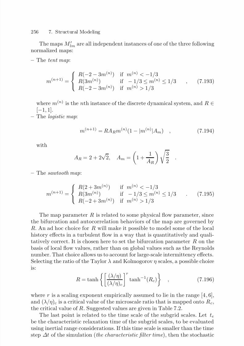
7/21/2019 Large Eddy Simulation for Incompressible Flows
http://slidepdf.com/reader/full/large-eddy-simulation-for-incompressible-flows 278/573
256 7. Structural Modeling
The maps M lm are all independent instances of one of the three followingnormalized maps:
– The tent map:
m(n+1) =
R(−2 − 3m(n)) if m(n) < −1/3R(3m(n)) if − 1/3 ≤ m(n) ≤ 1/3R(−2 − 3m(n)) if m(n) > 1/3
, (7.193)
where m(n) is the nth instance of the discrete dynamical system, and R ∈[−1, 1].
– The logistic map:
m(n+1) = RARm(n)(1 − |m(n)|Am) , (7.194)
with
AR = 2 + 2√
2, Am =
1 +
1
AR
3
2 .
– The sawtooth map:
m(n+1) =
R(2 + 3m(n)) if m(n) < −1/3R(3m(n)) if − 1/3 ≤ m(n) ≤ 1/3R(−2 + 3m(n)) if m(n) > 1/3
. (7.195)
The map parameter R is related to some physical flow parameter, sincethe bifurcation and autocorrelation behaviors of the map are governed byR. An ad hoc choice for R will make it possible to model some of the localhistory effects in a turbulent flow in a way that is quantitatively and quali-
tatively correct. It is chosen here to set the bifurcation parameter R on thebasis of local flow values, rather than on global values such as the Reynoldsnumber. That choice allows us to account for large-scale intermittency effects.Selecting the ratio of the Taylor λ and Kolmogorov η scales, a possible choiceis:
R = tanh
(λ/η)
(λ/η)c
rtanh−1(Rc)
, (7.196)
where r is a scaling exponent empirically assumed to lie in the range [4, 6],
and (λ/η)c is a critical value of the microscale ratio that is mapped onto Rc,the critical value of R. Suggested values are given in Table 7.2.The last point is related to the time scale of the subgrid scales. Let te
be the characteristic relaxation time of the subgrid scales, to be evaluatedusing inertial range considerations. If this time scale is smaller than the timestep ∆t of the simulation (the characteristic filter time ), then the stochastic

7/21/2019 Large Eddy Simulation for Incompressible Flows
http://slidepdf.com/reader/full/large-eddy-simulation-for-incompressible-flows 279/573
7.7 Explicit Evaluation of Subgrid Scales 257
Table 7.2. Parameters of the Chaotic Map Model.
Map Rc (λ/η)c r
Logistic −(2 + 2√ 2)1/2 26 5
Tent -1/3 28.6 5
Sawtooth -1/3 28.6 5
variables M i must be updated nu times per time step, with
nu ≈ ∆tte= ∆t|∇u|f M
Re−1/3∆ , (7.197)
where f M is a fundamental frequency associated with the chaotic maps usedto generate the variables. It is defined as:
f M = C
θ , (7.198)
where C is some positive constant and θ the integral iteration scale
θ = 1
2ρ(0) +
l=1,∞
ρ(l), ρ(l) = m(n)m(n+l)
m(n)m(n) , (7.199)
which completes the description of the model. This model is Galilean- andframe-invariant, and automatically generates realizable Reynolds stresses. Itreproduces the desired root-mean-square amplitude of subgrid fluctuations,along with the probability density function for this amplitude. Finally, theproper temporal auto-correlation function can be enforced.
7.7.3 Kerstein’s ODT-Based Method
A more complex chaotic map model based on Kerstein’s One-DimensionalTurbulence (ODT) approach11 was also proposed [650, 387, 389, 390, 388,305, 306, 208, 198, 386, 771]. This is a method for simulating turbulent fluc-tuations along one-dimensional lines of sight through a three-dimensionalturbulent flows. The velocity fluctuations evolve by two mechanisms, namelythe molecular diffusion and turbulent stirring. The latter mechanisms is takeninto account by a sequence of fractal transformations denoted eddy events.An eddy event may be interpreted as a model of an individual eddy, whoselocation, length scale and frequency are determined using a non-linear prob-abilistic model.
11 It is worth noting that ODT originates in the Linear Eddy Model [384, 385, 117,118, 177, 696, 414, 413, 473].
7/21/2019 Large Eddy Simulation for Incompressible Flows
http://slidepdf.com/reader/full/large-eddy-simulation-for-incompressible-flows 280/573
258 7. Structural Modeling
The diffusive step consists in solving the following one-dimensional ad-vection-diffusion equation for each subgrid velocity component along the line
∂ui∂t
+ ∂ ∂xj
(V jui) = ∂p∂xi
+ ν ∂ 2ui∂x2
, (7.200)
where ν is the molecular viscosity and V is the local advective field such that
ui =
Ω
V i(ξ )dξ , (7.201)
where Ω is the volume based on the cutoff length ∆.The second step, which accounts for non-linear effects, is more complex
and consists in two mathematical operations. The first one is a measure-preserving map representing the turbulent stirring, while the second one isa modification of the velocity profiles in order to implement energy transfersamong velocity components. These two steps can be expressed as
ui(x) ←− ui(f (x)) + ciK (x) , (7.202)
where the stirring-related mapping f (x) is defined as
f (x) = x0 +
3(x − x0) if x0 ≤ x ≤ x0 + l/32l − 3(x − x0) if x0 + l/3 ≤ x ≤ x0 + 2l/33(x − x0) − 2l if x0 + 2l/3 ≤ x ≤ x0 + lx − x0 otherwise
(7.203)
where l is the length of the segment affected by the eddy event. The secondterm in the right hand side of (7.202) is implemented to capture pressure-induced energy redistribution between velocity components and thereforemakes it possible to account for the return to isotropy of subgrid fluctua-tions. The kernel K is defined as
K (x) = x − f (x) (7.204)
The amplitude coefficients ci are determined for each eddy to enforce thetwo following constraints: (i) the total subgrid kinetic energy E =
i E i =
i12
ui(x)ui(x)dx remains constant, and (ii) the subgrid scale spectrum
must be realizable, i.e. the energy extracted from a velocity component cannotexceed the available energy in this component. The resulting definition of thecoefficients is
ci = 27
4l
−wi + sign(wi)
(1 − α)w2
i + α
2
j=i
w2j
, (7.205)

7/21/2019 Large Eddy Simulation for Incompressible Flows
http://slidepdf.com/reader/full/large-eddy-simulation-for-incompressible-flows 281/573
7.7 Explicit Evaluation of Subgrid Scales 259
where
wi =
1
l2 u
i(f (x))K (x)dx =
4
9l2 x0+l
x0 u
i(x)(l − 2(x − x0))dx . (7.206)
The degree of energy redistribution is governed by the parameter α, whichis taken equal to 2/3 in Ref. [650] (corresponding to equipartition of theavailable energy among the velocity components).
The last element of the method is the eddy selection step, which giveaccess to the time sequence of eddy events. All events are implemented in-stantaneously, but occur with frequencies comparable to turnover frequenciesof associated turbulent structures. At each time step, the event-rate distri-
bution is obtained by first associating a time scale τ (x0, l) with every eddyevent. Using l/τ and l3/τ 2 as an eddy velocity scale and a measure of theenergy of the eddy motion, respetively, the time scale τ is computed usingthe following relation
l
τ
2
∼ (1 − α)w21 +
α
2(w2
2 + w23) − Z
ν 2
l2 , (7.207)
where Z is the amplitude of the viscous penalty term that governs the sizeof the smallest eddies for given local strain conditions. A probabilistic model
can be derived defining an event-rate distribution λ
λ(x0, l , t) = C
l2τ (x0, l , t) , (7.208)
where C is an arbitrary parameter which determines the relative strength of turbulent stirring.
7.7.4 Kinematic-Simulation-Based Reconstruction
Following Flohr and Vassilicos [220], the incompressible, turbulent-like sub-grid velocity field is generated by summing different Fourier modes
u(x, t) =n=1,N
(an cos(kn · x + ωnt) + bn sin(kn · x + ωnt)) , (7.209)
where N is the number of Fourier modes, an and bn are the amplitudescorresponding to wave vector kn, and ωn is a time frequency. The wavevectors are randomly distributed in spherical shells:
kn = kn(sin θ cos φ, sin θ sin φ, cos θ) , (7.210)
where θ and φ are uniformly distributed random angles within [0, 2π[ and[0, π], respectively. The random uncorrelated amplitude vectors an and bn
7/21/2019 Large Eddy Simulation for Incompressible Flows
http://slidepdf.com/reader/full/large-eddy-simulation-for-incompressible-flows 282/573
260 7. Structural Modeling
are chosen such that
an · kn = bn · kn = 0 , (7.211)
to ensure incompressibility, and
|an|2 = |bn|n = 2E (kn)∆kn , (7.212)
where E (k) is the prescribed energy spectrum, and ∆kn is the wave num-ber increment between the shells. Recommended shell distributions in thespectral space are:
– Linear distribution
kn = k1 + kN − k1
N − 1 (n − 1) ; (7.213)
– Geometric distribution
kn = k1
kN k1
(n−1)/(N −1)
; (7.214)
– Algebraic distribution
kn = k1nlog(kN /k1)/ logN . (7.215)
The time frequency ωn is arbitrary. Possible choices are ωn = U ckn if allthe modes are advected with a constant velocity U c, and ωn =
k3nE (kn) if
it is proportional to the eddy-turnover time of mode n.In practice, Flohr and Vassilicos use this model to evaluate the dynamics
of a passive tracer, but do not couple it with the momentum equations.
Nevertheless, it could be used to close the momentum equation too.
7.7.5 Velocity Filtered Density Function Approach
The reconstruction of the subgrid motion via a stochastic system which obeysthe required probability density function is proposed by Gicquel et al. [264].This method is also equivalent (up to the second order) to solving the differ-ential equations for the subgrid stresses presented in Sect. 7.5.3. The basesof the method are presented in this section, and will not be repeated here.
The key of the present method is the definition of a Lagrangian MonteCarlo method, which is used to evaluate both the position X i (in space) andthe value of a surrogate of the subgrid velocity, U i, associated to a set of virtual particules. The value of the subgrid velocity in each cell of the Large-Eddy Simulation grid is defined as the statistical average over all the virtualparticules that cross the cell during a fixed time interval.
7/21/2019 Large Eddy Simulation for Incompressible Flows
http://slidepdf.com/reader/full/large-eddy-simulation-for-incompressible-flows 283/573
7.7 Explicit Evaluation of Subgrid Scales 261
The stochastic differential equations equivalent to the first model pre-sented in Sect. 7.5.3 is
dX i(t) = U i(t)dt , (7.216)
d U i(t) =
− ∂p
∂xi+ 2ν
∂sik∂xk
+ Gij( U j(t) − uj(t))
dt
+
C 0ε dW vi (t) , (7.217)
where Gij , C 0 and ε are defined in Sect. 7.5.3, and W vi denotes and indepen-dent Wiener–Levy process.
The second model proposed by Gicquel accounts for viscous diffusion andis expressed as
dX i(t) = U i(t)dt +√
2ν dW xi (t) , (7.218)
d U i(t) =
− ∂p
∂xi+ 2ν
∂sik∂xk
+ Gij( U j(t) − uj(t))
dt
+ C 0ε dW v
i
(t) +√
2ν ∂ui
∂xjdW x
j
(t) , (7.219)
where ν is the molecular viscosity and W xi is another independent Wiener–Levy process. In practice, convergence of the statistical average over the par-ticules within each cell must be carefully checked to recover reliable results.
7.7.6 Subgrid Scale Estimation Procedure
A two-step subgrid scale estimation procedure in the physical space12 is pro-
posed by Domaradzki and his coworkers [458, 187, 394, 188]. In the first(kinematic) step, an approximate inversion of the filtering operator is per-formed, providing the value of the defiltered velocity field on the auxiliarygrid. In the second (non-linear dynamic) step, scales smaller than the filterlength associated to the primary grid are generated, resulting in an approxi-mation of the full solution.
Let u be the filtered field obtained on the primary computational grid,and u• the defiltered field on the secondary grid. That secondary grid ischosen such that the associated mesh size is twice as fine as the mesh size
of the primary grid. We introduce the discrete filtering operator Gd, definedsuch that
Gdu• = u . (7.220)
12 A corresponding procedure in the spectral space is described in reference [190].

7/21/2019 Large Eddy Simulation for Incompressible Flows
http://slidepdf.com/reader/full/large-eddy-simulation-for-incompressible-flows 284/573
262 7. Structural Modeling
It is important to note that in this two-grid implementation, the right-hand side of equation (7.220) must first be interpolated on the auxiliary gridto recover a well-posed linear algebra problem. To avoid this interpolationstep, Domaradzki proposes to solve directly the filtered Navier–Stokes equa-tions on the finest grid, and to define formally the G filtering level by taking∆ = 2 ∆. The defiltered field u• is obtained by solving the inverse problem
u• = (Gd)−1u . (7.221)
This is done in practice by solving the corresponding linear system. Inpractice, the authors use an three-point discrete approximation of the boxfilter for Gd (see Sect. 13.2 for a description of discrete test filters). Thisstep corresponds to an implicit deconvolution procedure (the previous oneswere explicit procedures, based on the construction of the inverse operatorvia Taylor expansions or iterative procedures), and can be interpreted as aninterpolation step of the filtered field on the auxiliary grid.
The ua subgrid velocity field is then evaluated using an approximation of
its associated non-linear production term:
ua = θa N , (7.222)
where θa and N are a characteristic time scale and N the production rate.These terms are evaluated as follows. The full convection term on the auxil-iary grid is
−u•j∂u•i∂xj
, j = 1, 2, 3 . (7.223)
This term accounts for the production of all the frequencies resolved onthe auxiliary grid. Since we are interested in the production of the smallscales only, we must remove the advection by the large scales, and restrict
the resulting term tho the desired frequency range. The resulting term N i is
N i = (Id − G)
−(u•j − uj)
∂u•i∂xj
. (7.224)
In practice, the convolution filter G is replaced by the discrete operatorGd. The production time θa is evaluated making the assumption that thesubgrid kinetic energy is equal to the kinetic energy contained in the smallestresolved scales:
|ua|2 = θ2
a|N |2 = α2|u• − u|2 =⇒ θa = α2|u• − u|
|N | , (7.225)
where α is a proportionality constant, nearly equal to 0.5 for the box filter.This completes the description of the model.

7/21/2019 Large Eddy Simulation for Incompressible Flows
http://slidepdf.com/reader/full/large-eddy-simulation-for-incompressible-flows 285/573
7.7 Explicit Evaluation of Subgrid Scales 263
7.7.7 Multi-level Simulations
This class of simulation relies on the resolution of an evolution equation
for ua on the auxiliary grid. These simulations can be analyzed within theframework of the multiresolution representation of the data [293, 295, 17,294], or similar theories such as the Additive Turbulent Decomposition [471,338, 80].
Let us consider N filters G1,...,GN , with associated cutoff lengths ∆1 ≤... ≤ ∆N . We define the two following sets of velocity fields:
un = Gn ... G1 u = Gn1 u , (7.226)
v
n
= u
n
− u
n+1
= (Gn
1 − Gn+1
1 ) u = F n u . (7.227)The fields un and vn are, respectively, the resolved field at the nth level
of filtering and the nth level details. We have the decomposition
un = un−k +l=1,k
vn−l , (7.228)
yielding the following multiresolution representation of the data:
u
≡ uN , v1,..., vN −1
. (7.229)
The multilevel simulations are based on the use of embedded computa-tional grids or a hierarchical polynomial basis to solve the evolution equationsassociated with each filtering level/details level. The evolution equations areexpressed as
∂ un
∂t + NS (un) = −τ n = −[Gn1 , NS ](u), n ∈ [1, N ] , (7.230)
where
NS is the symbolic Navier–Stokes operator and [., .] the commutator
operator. The equations for the details are
∂ vn
∂t + NS (vn) = −τ n = −[F n, NS ](u), n ∈ [1, N − 1] , (7.231)
or, equivalently,
∂ vn
∂t + NS (un) − NS (un+1) = −τ n + τ n+1, n ∈ [1, N − 1] . (7.232)
There are three possibilities for reducing the complexity of the simulation
with respect to Direct Numerical Simulation:
– The use of a cycling strategy between the different grid levels. Freezing thehigh-frequency details over some time while integrating the equations forthe low-frequency part of the solution results in a reduction of the simula-tion complexity. This is referred to as the quasistatic approximation for the

7/21/2019 Large Eddy Simulation for Incompressible Flows
http://slidepdf.com/reader/full/large-eddy-simulation-for-incompressible-flows 286/573
264 7. Structural Modeling
high frequencies. The main problem associated with the cycling strategy isthe determination of the time over which the high frequencies can be frozenwithout destroying the quality of the solution. Some examples of such a cy-cling strategy can be found in the Multimesh method of Voke [736], theNon-Linear Galerkin Method [174, 579, 705, 222, 223, 224, 91], the Incre-mental Unknowns technique [73, 201, 128, 200], Tziperman’s MTS algo-rithm [722], Liu’s multigrid method [452, 453] and the Multilevel algorithmproposed by Terracol et al. [711, 710, 633].
– The use of simplified evolution equations for the details instead of (7.231).A linear model equation is often used, which can be solved more easily thanthe full nonlinear mathematical model. Some examples among others arethe Non-Linear Galerkin method, early versions of the Variational Multi-
scale approach proposed by Hughes et al. [332, 331, 336, 335, 333, 334],and the dynamic model of Dubrulle et al. [203, 426]. Another possibilityis to assume that the nth-level details are periodic within the filtering cellassociated with the (n − 1)th filtering level. Each cell can then be treatedseparately from the others. An example is the Local Galerkin method of McDonough [468, 466, 467]. It is interesting to note that this last assump-tion is shared by the Homogenization approach developed by Perrier andPironneau (see Sect. 7.2.3). Menon and Kemenov [382] use a simplifiedset of one-dimensional equations along lines. A reminiscent approach was
developed by Kerstein on the grounds of the stochastic One-DimensionalTurbulence (ODT) model (presented in Sect. 7.7.3).
– The use of a limited number of filtering levels. In this case, even at the finestdescription level, subgrid scales exist and have to be parametrized. The gainis effective because it is assumed that simple subgrid models can be usedat the finest filtering level, the associated subgrid motion being closer toisotropy and containing much less energy than at the coarser filtering levels.Examples, among others, are the Multilevel algorithm of Terracol [710,633], the Modified Estimation Procedure of Domaradzki [193, 183], and
the Resolvable Subfilter Scales (RSFS) model [806].
Some strategies combining these three possibilities can of course be de-fined. The efficiency of the method can be further improved by using a localgrid refinement [699, 62, 378]. Non-overlapping multidomain techniques canalso be used to get a local enrichment of the solution [611, 633]. These meth-ods are presented in Chap. 11.
We now present a few multilevel models for large-eddy simulation. Theemphasis is put here on methods based on two grid levels, and which can beinterpreted as models, in the sense that they rely on some simplifications andcannot be considered just as multilevel algorithms applied to classical large-eddy simulations. In these methods, the secondary grid level is introduced tocompute the fluctuations u, and not for the purpose of reducing the cost of the primary grid computation. This latter class of methods, which escapesthe simple closure problem, is presented in Chap. 11. It is worth noting that

7/21/2019 Large Eddy Simulation for Incompressible Flows
http://slidepdf.com/reader/full/large-eddy-simulation-for-incompressible-flows 287/573
7.7 Explicit Evaluation of Subgrid Scales 265
Fig. 7.3. Schematic of the three-level models. Left : spectral decomposition; Middle :computational grid; Right : time cycling.
these two-grid methods correspond to a three-level decomposition of the exact
solution: two filters are applied in order to split the exact solution into threespectral bands (see Fig. 7.3).
Using Harten’s representation (7.229), this decomposition is expressed as
u = u2,v1,v0 , (7.233)
where u2 is the resolved filtered field at the coarsest level, u1 = u2 + v1 isthe resolved filtered field at the finest level, and v0 is the unresolved field atthe finest level, i.e. the true subgrid velocity field. The detail v1 correspondsto the part of the unresolved field at the coarsest level which is resolved atthe finest filtering level.
The coupling between these three spectral bands and the associated clo-sure problem can be understood by looking at the nonlinear term. For thesake of simplicity, but without restricting the generality of the results, we willassume here that the filtering operators perfectly commute with differentialoperators, and that the domain is unbounded. The remaining coupling comesfrom the nonlinear convective term. For the exact solution, it is expressed as
B (u,u) = B (u2 + v1 + v0, u2 + v1 + v0) , (7.234)
where B is the bilinear form defined by relation (3.27).At the coarsest resolution level, the nonlinear term can be split as follows:
B (u,u)2
= B (u2,u2)2
I

7/21/2019 Large Eddy Simulation for Incompressible Flows
http://slidepdf.com/reader/full/large-eddy-simulation-for-incompressible-flows 288/573
266 7. Structural Modeling
+ B(u2, v1)2
+ B(v1, u2)2
+ B(v1, v1)2
II
+ B(u2 + v1, v0)2
+ B(v0, u2 + v1 + v0)2
III
. (7.235)
Term I can be computed directly at the coarsest grid level. Term II represents the direct coupling between the two levels of resolution, and canbe computed exactly during the simulation. Term III represents the directcoupling with the true subgrid modes. It is worth noting that, at least theo-retically, the non-local interaction between u2 and v 0 is not zero and requiresthe use of an ad hoc subgrid model.
At the finest resolution level, the analogous decomposition yields
B(u, u)1
= B(u2, u2)1
IV
+ B(u2, v1)1
+ B(v1, u2)1
V
+ B(v1
,v1
)
1 V I
(7.236)
+ B(u2 + v1, v0)1
+ B(v0, u2 + v1)1
+ B(v0, v0)1
V II
.
Terms I V and V represent the coupling with the coarsest resolution level,and can be computed explicitly. Term V I is the nonlinear self-interaction of the detail v1, while term V II is associated with the interaction with subgridscales v0 and must be modeled.
By looking at relations (7.235) and (7.236), we can see that specific sub-grid models are required at each level of resolution. Several questions arisedealing with this closure problem:
1. Is a subgrid model necessary in practice for terms III and V II ?2. What kind of model should be used?3. Is it possible to use the same model for both terms?
Many researchers have worked on these problems, leading to the definitionof different three-level strategies. A few of them are presented below:
1. The Variational Multiscale Method (VMS) proposed by Hughes et al.(p. 267).
2. The Resolvable Subfilter-scale Model (RSFR) of Zhou et al. (p. 269).3. The Dynamic Subfilter-scale Model (DSF) developed by Dubrulle et al.
(p. 270).

7/21/2019 Large Eddy Simulation for Incompressible Flows
http://slidepdf.com/reader/full/large-eddy-simulation-for-incompressible-flows 289/573
7.7 Explicit Evaluation of Subgrid Scales 267
4. The Local Galerkin Approximation (LGA), as defined by McDonough etal. (p. 270).
5. The Two-Level-Simulation (TLS) method, proposed by Menon et al.(p. 271).
6. The Modified Subgrid-scale Estimation Procedure (MSEP) of Doma-radzki et al. (p. 269).
7. Terracol’s multilevel algorithm (TMA) with explicit modeling of term III (p. 271).
The underlying coupling strategies are summarized in Table 7.3.
Table 7.3. Characteristics of multilevel subgrid models. + means that the term istaken into account, and − that it is neglected.
Model I II III IV V VI VII
VMS + + − + + + +RSFR + + − + + + +MSEP + + − + + + −DSF + + − + + − −LGA + + − − + + −TLS + + − − + + −TMA + + + + + + +
Variational Multiscale Method. Hughes et al. [332, 331, 336, 335, 333,334] first introduced the Variational Multiscale Method within the frameworkof finite element methods, and then generalized it considering a fully generalframework.
The coupling term I II is neglected (see Table 7.3), at least in the originalformulation of the method. The need for a full coupling including term III
was advocated by Scott Collis [660].In practical applications, the coarse resolution cutoff length scale ∆
2is
taken equal to twice the fine resolution cutoff length scale ∆1
, and the solutionis integrated with the same time step at the two levels.
The subgrid term V II is parametrized using a Smagorinsky-like func-tional model
(V II )ij = −2ν sgs
∂v1j
∂xi+
∂v1i
∂xj
, (7.237)
with two possible variants:
– The small–small model13:
13 This form of the dissipation is very close to the variational embedded stabiliza-tion previously proposed by Hughes (see Sect. 5.3.4). Similar expressions for thedissipation term have been proposed by Layton [429, 428] and Guermond [280].

7/21/2019 Large Eddy Simulation for Incompressible Flows
http://slidepdf.com/reader/full/large-eddy-simulation-for-incompressible-flows 290/573
268 7. Structural Modeling
ν sgs = (C S∆1)2
2|S 1|, S 1ij =
∂v1j
∂xi+
∂v1i
∂xj
. (7.238)
– The large–small model:
ν sgs = (C S∆1)2
2|S
1|, S 1ij =
∂u1j
∂xi+
∂u1i
∂xj
. (7.239)
The recommended value of the constant C S is 0.1 for isotropic turbulenceand plane channel flow. This value is arbitrary, and numerical experimentsshow that it could be optimized.
Numerical results show that both variants lead to satisfactory results onacademic test cases, including non-equilibrium flow. This can be explained by
the fact that the subgrid tensor is evaluated using the S 1 tensor, instead of S 2
in classical subgrid-viscosity methods. Thus, the subgrid model dependencyis more local in Fourier space, the emphasis being put on the highest resolvedfrequency, yielding more accurate results (see Sect. 5.3.3).
This increased localness in terms of wavenumber with respect to the usualSmagorinsky model is emphasized rewriting the VMS method as a specialclass of hyperviscosity models. The link between these two approaches isenlightened assuming that the following differential approximation for sec-ondary filter utilized to operate the splitting u1 = u2 + v1 holds14:
u2 = G2 u1 (Id + α∆22∇2)u1 (7.240)
where α is a filter-dependent parameter, yielding
v1 = −α∆2
2∇2u1 (7.241)
Inserting that definition for v1 into previous expressions for both theSmall-Small (7.238) and the Large-Small (7.239) models shows that these
models are equivalent to fourth-order hyperviscosity models (see p. 121).Higher-order hyperviscosities are recovered using higher-order elliptic filtersto operate the splitting.
The splitting of the resolved field into two parts can be interpreted asthe definition of a more complex accentuation technique (see Sect. 5.3.3, p.156). In the parlance of Hughes, the filtered Smagorinsky model correspondsthe the Small-Large model (while the classical Smagorinsky model is theLarge-Large model).
The accuracy of the results is observed to depend on the spectral proper-
ties of the filter used to extract v1 from u1. It is observed that kinetic energypile-up can occur if a spectral sharp cutoff is utilized. The reason why is thatin this case the subgrid viscosity acts only on scales encompassed within v1
14 It is known from results of Sect. 2.1.6 that this approximation is valid for smoothsymmetric filters and for most discrete filters.

7/21/2019 Large Eddy Simulation for Incompressible Flows
http://slidepdf.com/reader/full/large-eddy-simulation-for-incompressible-flows 291/573
7.7 Explicit Evaluation of Subgrid Scales 269
and non-local energy transfers between largest scales and v0 are neglected.The use of a smooth filter which allows a frequency overlap between u1 andv1 alleviates this problem.
The use of the classical Smagorinsky model may also lead to an excessivedamping of scales contained in v1. To cure this problem, Holmen et al. [316]proposed to use the Germano-Lilly procedure to evaluate the constant of theLarge-Small model.
Another formulation for the Variational Multiscale Method is proposedby Vreman [745] who build some analogous models on the grounds of the testfilter G2. Keeping in mind that one essential feature of the VMS approach isthat the action of the subgrid scale is restricted to the small scale field v1,the following possibilities arise
– Model 1: restriction of the usual Smagorinsky model
(V II )ij = (Id − G2)
−2(C S ∆
1)2
2|S
1|S 1ij
. (7.242)
– Model 2 : Smagorinsky model based on the small scales
(V II )ij = −2(C S ∆1
)2 2|S 1|S
1ij . (7.243)
– Model 3 : restriction of the Smagorinsky model based on the small scales
(V II )ij = (Id − G2) −2(C S ∆
1)2
2|S 1|S 1ij
. (7.244)
Models 2 and 3 are equivalent if the filter G2 is a sharp cutoff filter, butare different in the general case. If a differential second-order elliptic filter isused, model 3 will be equivalent to a sixth-order hyperviscosity, while model2 is associated to a fourth-order hyperviscosity.
Resolvable Subfilter-scale Model. Zhou, Brasseur and Juneja [806] de-veloped independently a three-level model which is almost theoretically equiv-alent to the Variational Multiscale Method of Hughes. The terms taken intoaccount at the two resolution levels are the same (term III is ignored inboth cases), and term V II is modeled using the Smagorinsky model. Themodel used is the small–small model (7.238) following Hughes’ terminology.As in the VMS implementation described above, simulations of homogeneous
anisotropic turbulence are carried out with ∆
2
= 2∆
1
.Modified Subgrid-scale Estimation Procedure. Domaradzki et al. [782,193, 183] proposed a modification of the original subgrid-scale estimationprocedure (see Sect. 7.7.6) in order to improve its robustness. The key point

7/21/2019 Large Eddy Simulation for Incompressible Flows
http://slidepdf.com/reader/full/large-eddy-simulation-for-incompressible-flows 292/573
270 7. Structural Modeling
of this method is to account directly for the production of small scales v 1 bythe forward energy cascade rather than using the production estimate (7.222).
The governing equations of this method are the same as those of VMS andRSFR, with the exception that the subgrid term V II in the detail equation isneglected. The main difference with VMS and RSFR is the time integrationprocedure: in the two previous approaches the coarsely and finely resolvedfields are advanced at each time step, while Domaradzki and Yee proposedadvancing the fine grid solution u1 over an evolution time T between 1% and3% of the large-eddy turnover time.
Dynamic Subfilter-scale Model. The dynamic subfilter-scale model of Dubrulle et al. [203, 426] appears as a linearized version of the three-level
approach: the nonlinear term V I in the evolution equation of the details isneglected, and the subgrid term V II is not taken into account. This lin-earization process renders the detail equation similar to those of the RapidDistortion Theory. Only a priori tests have been carried out on parallel wall-bounded flows.
Local Galerkin Approximation. The Local Galerkin Approach proposedby McDonough et al. [468, 466, 467, 470, 471] can be seen as a simplificationof a typical three-level model. All subgrid terms are neglected, and, due to thefact that the original presentation of the method is not based on a filtering
operator, term IV is not taken into account.The key idea of the method is to make the assumption that the fluctuating
field v1 is periodic in space within each cell associated with the coarse levelresolution (see Fig. 7.4). Consequently, a spectral simulation is performed
within each cell of size ∆2
, but the field v1 is not continuous at the interface of
each cell. The number of Fourier modes determine the cutoff length scale ∆1
.
Fig. 7.4. Schematic of the Local Galerkin Approach.
7/21/2019 Large Eddy Simulation for Incompressible Flows
http://slidepdf.com/reader/full/large-eddy-simulation-for-incompressible-flows 293/573
7.7 Explicit Evaluation of Subgrid Scales 271
This method can be seen as a dynamic extension of the Kinematic Sim-ulation approach (see Sect. 7.7.4) and is very close, from a practical point of view, to the Perrier–Pironneau homogenization technique (see Sect. 7.2.3).
Menon’s Two-Level-Simulation Method. Menon and Kemenov [382]developed a two-level method based on a simplified model for the subgridscales. Instead of defining a three-dimensional grid to compute the subgridmodes inside each cell of the large-eddy simulation grid, the authors chose tosolve simplified one-dimensional equations along lines (one in each directionin practice) inside each cell, leading to a large cost reduction. This featuremakes it reminiscent of the Kerstein subgrid closure based on the stochasticODT model (see Sect. 7.7.3). In Menon’s approach, terms III and V II are
neglected.In each cell, the three-dimensional subgrid velocity field is modeled asa family of one-dimensional velocity vector fields defined on the underlyingfamily of lines l1, l2, l3 (which are in practice aligned with the axes of thereference Cartesian frame). Assuming that the derivatives of the modeledsubgrid velocity field are such that
∂v1i
∂l1∼ ∂v1
i
∂l2∼ ∂v1
i
∂l3, i = 1, 2, 3 , (7.245)
and that the incompressibility constraint can be expressed as
∂
∂lj
v1
1,j + v12,j + v1
3,j
= 0 , (7.246)
where v1k,j refers to the jth component of the subgrid field computed along
the line of index k, the following mometum-like equations are found:
∂v1
i,j∂t + N L(v1i,j , u, lj) = −∂p
1
∂lj+ 3ν
∂ 2v1
i,j∂l2j
, (7.247)
where the non-linear term N L(v1i,j , u, lj) contains the surrogates for terms
IV , V and V I .
Terracol’s Multilevel Algorithm. The last three-level model presented inthis section is the multilevel closure proposed by Terracol et al. [710, 633, 711].It is the only one which considers the full closure problem by taking intoaccount the non-local interaction term III , and can then be considered as
the most general one. The original method presented in [711] is able to handlean arbitrary number of filtering levels, but the present presentation will berestricted to the three-level case.
7/21/2019 Large Eddy Simulation for Incompressible Flows
http://slidepdf.com/reader/full/large-eddy-simulation-for-incompressible-flows 294/573
272 7. Structural Modeling
The key points of the method are:
– The use of a specific closure at each level u2 and u1. The proposed model at
the coarse level is an extension of the one-parameter dynamic mixed model(see Sect. 7.4.2, p. 240), where the scale-similarity part is replaced by theexplicitly computable term II . Term III is modeled using the Smagorin-sky part of the mixed dynamic model, with a dynamically computed con-stant. At the fine resolution level, term V II is parametrized using a one-parameter dynamic mixed model. Numerical results demonstrate that theuse of a specific model for term III is mandatory, since the use of a classicaldynamic Smagorinsky model yields poor results.
– The definition of a cycling strategy between the different resolution levels,
in order to decrease the computational cost while maintaining the accuracyof the results. The idea is here to freeze the details v 1 and to carry out thecomputation at the coarse level only during a time T .15 The problem is tofind the optimal T in order to maximize the cost reduction while limitingthe loss of coherence between u2 and v1. A simple solution is to advancethe solution for one time step at each level, alternatively, with the samevalue of the Courant number at each level. Numerical experiments showthat this solution leads to good results with a gain of about a factor two.
Results obtained using this method on a plane mixing layer configuration
are illustrated in Fig. 7.5.
7.8 Direct Identification of Subgrid Terms
Introduction. This section is dedicated to the presentation of approacheswhich aim at reconstructing the subgrid terms using direct identificationmathematical tools.
Like all other subgrid models, either of functional or structural types, they
answer the following question: given a filtered velocity field u, what is thesubgrid acceleration? Subgrid models described previously were all based onsome a priori knowledge of the nature of the interactions between resolvedand subgrid scales, on a description of the filter, or on a structure of thesubgrid scales hypothesized a priori. The models presented in this sectiondo not require any of this information, and do not rely on any assumptionsabout the internal structure of the subgrid modes.
They are based on mathematical tools which are commonly used withinthe framework of pattern recognition, and do not really correspond to what
is usually called a “model”. Using Moser’s words, they represent a radical approach to large-eddy simulation.
15 This part is close to the quasistatic approximation for small scales introducedwithin the context of the nonlinear Galerkin method [174].
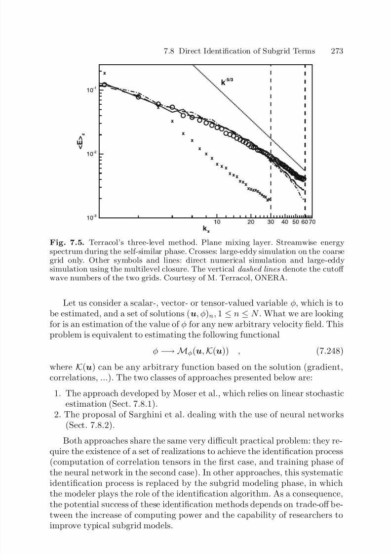
7/21/2019 Large Eddy Simulation for Incompressible Flows
http://slidepdf.com/reader/full/large-eddy-simulation-for-incompressible-flows 295/573
7.8 Direct Identification of Subgrid Terms 273
Fig. 7.5. Terracol’s three-level method. Plane mixing layer. Streamwise energyspectrum during the self-similar phase. Crosses: large-eddy simulation on the coarsegrid only. Other symbols and lines: direct numerical simulation and large-eddysimulation using the multilevel closure. The vertical dashed lines denote the cutoff wave numbers of the two grids. Courtesy of M. Terracol, ONERA.
Let us consider a scalar-, vector- or tensor-valued variable φ, which is tobe estimated, and a set of solutions (u, φ)n, 1 ≤ n ≤ N . What we are lookingfor is an estimation of the value of φ for any new arbitrary velocity field. Thisproblem is equivalent to estimating the following functional
φ −→Mφ(u,K(u)) , (7.248)
where K(u) can be any arbitrary function based on the solution (gradient,correlations, ...). The two classes of approaches presented below are:
1. The approach developed by Moser et al., which relies on linear stochasticestimation (Sect. 7.8.1).
2. The proposal of Sarghini et al. dealing with the use of neural networks(Sect. 7.8.2).
Both approaches share the same very difficult practical problem: they re-quire the existence of a set of realizations to achieve the identification process(computation of correlation tensors in the first case, and training phase of the neural network in the second case). In other approaches, this systematic
identification process is replaced by the subgrid modeling phase, in whichthe modeler plays the role of the identification algorithm. As a consequence,the potential success of these identification methods depends on trade-off be-tween the increase of computing power and the capability of researchers toimprove typical subgrid models.

7/21/2019 Large Eddy Simulation for Incompressible Flows
http://slidepdf.com/reader/full/large-eddy-simulation-for-incompressible-flows 296/573
274 7. Structural Modeling
7.8.1 Linear-Stochastic-Estimation-Based Model
Moser et al. [419, 549, 548, 165, 296, 741, 797] proposed an identification
procedure based on Linear Stochastic Estimation. This approach can be in-terpreted in several ways. An important point is that it is closely tied to thedefinition of large-eddy simulation as an optimal control problem, where thesubgrid model plays the role of a controller. This interpretation is discussedin Sect. 9.1.4 and will not be repeated here. The linear stochastic estimationapproach can also be seen as the best linear approximation for the subgridterm in the least-squares sense. Starting from the general formulation (7.248),the linear estimation is written as
Mφ(E ) = φ + L · E T , with E = (u, K(u)) , (7.249)
where the tensorial dimension of L depends on those of φ, u and K(u). Thelinear stochastic estimation procedure leads to the best values of the coef-ficient of L in the least-squares sense. Considering vectorial unknowns, weobtain the following spatially non-local estimation
φi(x) = φi +
Lij(x, x)E j(x)dx ; (7.250)
the best coefficients Lij are computed by solving the following linear problem:
E i(x)φj(x) =
Ljk(x, x)E j(x)E k(x)dx . (7.251)
Local estimates can also be defined using one-point correlations insteadof two-point correlations to define L.
Practial applications of this approach have been carried out in homoge-neous turbulence and plane channel flow [549, 548]. Numerical experimentshave shown that both the subgrid stresses and the subgrid energy transfermust be taken into account to obtain stable and accurate numerical simu-lations. This means that both uiτ ij and S ijτ ij must be recovered. This isachieved by estimating the subgrid acceleration
φi = ∂
∂xjτ ij , (7.252)
as a function of the velocity field and its gradients
E = (u
, ∇u
) . (7.253)The mean value φ is computed from the original data set and stored.
In practice, some simplifications can be assumed in definitions (7.252) and(7.253) in parallel shear flows.

7/21/2019 Large Eddy Simulation for Incompressible Flows
http://slidepdf.com/reader/full/large-eddy-simulation-for-incompressible-flows 297/573
7.9 Implicit Structural Models 275
7.8.2 Neural-Network-Based Model
Sarghini et al. [645] proposed estimating the subgrid terms using a multilayer,
feed-forward neural network. Rather than estimating directly the subgridacceleration in the momentum equation, the authors decided to decrease thecomplexity of the problem by identifying the value of a subgrid-viscositycoefficient, yielding a new dynamic Smagorinsky model. To this end, a three-layer network is employed. The number of neurons in each layer is 15, 12and 6, respectively, with a single output (the subgrid viscosity). The inputvector is
E = (∇u, u ⊗ u) ∈ IR15 . (7.254)
The output is the subgrid model constant: φ = C S ∈ IR. The trainingof the neural network is achieved using data fields originating from a classi-cal large-eddy simulation of the same plane channel flow configuration. Thelearning rule used to adjust the weights and the biases of the network ischosen so as to minimize the summed-squared-error between the output of the network and the original set of data. Six thousand samples were foundnecessary for the training and validation steps. The training was performedthrough a backpropagation with weight decay technique in less than 500 it-erations.
A priori and a posteriori tests show that the resulting model leads tostable numerical simulations, whose results are very close to those obtainedusing typical subgrid viscosity models. An interesting feature of the model isthat the predicted subgrid viscosity exhibits the correct asymptotic behaviorin the near-wall region (see p. 159).
7.9 Implicit Structural Models
The last class of structural subgrid models discussed in this chapter is the im-plicit structural model family. These models are structural ones, i.e. they donot rely on any foreknowledge about the nature of the interactions betweenthe resolved scales and the subgrid scales. They can be classified as implicit,because they can be interpreted as improvements of basic numerical methodsfor solving the filtered Navier–Stokes equations, leading to the definition of higher-order accurate numerical fluxes. We note that, because the modifica-tion of the numerical method can be isolated as a new source term in themomentum equation, these models could also be classified as exotic formalexpansion models. A major specificity of these models is that they all aimat reproducing directly the subgrid force appearing in the momentum equa-tion, and not the subgrid tensor τ . They differ from the stabilized numericalmethods presented in Sect. 5.3.4 within the MILES framework because theyare not designed to induce numerical dissipation.
7/21/2019 Large Eddy Simulation for Incompressible Flows
http://slidepdf.com/reader/full/large-eddy-simulation-for-incompressible-flows 298/573
276 7. Structural Modeling
The two models presented in the following are:
1. The Local Average Method of Denaro (p. 276), which consists in a par-
ticular reconstruction of the discretized non-linear fluxes associated tothe convection term. This approach incorporates a strategy to filter thesubgrid-scale by means of an integration over a control volume and to re-cover the contribution of the subgrid scales with an integral formulation.It can be interpreted as a high-order space-time reconstruction procedurefor the convective numerical fluxes based on a defiltering process.
2. The Scale Residual Model of Maurer and Fey (p. 278). As for the Ap-proximate Deconvolution Procedure, the purpose is to evaluate the com-mutation error which defines the subgrid term. This evaluation is carried
out using the residual between the time evolution of the solutions of theNavier–Stokes equations on two different grids (i.e. at two different filter-ing levels) and assuming some self-similarity properties of this residual.This model can be considered as: (i) a generalization of the previous one,which does not involve the deconvolution process anymore, but requiresthe use of the second computational grid and (ii) a generalization of thescale-similarity models, the use of a test filter for defining the test fieldbeing replaced by the explicit computation (by solving the Navier–Stokesequations) of the field at the test filter level.
Other implicit approaches for large-eddy simulation exist, which make itpossible to obtain reliable results without subgrid scale model (in the com-mon sense given to that term), and without explicit addition of numericaldiffusion16. An example is the Spectro-Consistent Discretization proposed byVerstappen and Veldman [730, 729]. Because these approaches rely on nu-merical considerations only, they escape the modeling concept and will notbe presented here.
7.9.1 Local Average Method
An other approach to the traditional large-eddy simulation technique wasproposed by Denaro and his co-workers in a serie of papers [175, 169, 170].It is based on a space-time high-order accurate reconstruction/deconvolutionof the convective fluxes, which account for the subgrid-scale contribution.As a consequence, it can be seen as a particular numerical scheme based ona differential approximation of the filtering process. For sake of simplicity,we will present the method in the case of a dummy variable φ advected bya velocity field u, whose evolution equation is (only convective terms areretained):
∂φ
∂t = −∇ · (uφ) = A(u, φ) . (7.255)
16 Dissipative numerical methods should be classified as Implicit Functional Mod-eling.

7/21/2019 Large Eddy Simulation for Incompressible Flows
http://slidepdf.com/reader/full/large-eddy-simulation-for-incompressible-flows 299/573
7.9 Implicit Structural Models 277
The local average of φ in a filtering cell Ω is defined as the mean value of φ in this cell17:
φ(x, t) ≡ 1V Ω
φ(ξ, t)dξ = φ(t), ∀x ∈ Ω , (7.256)
where V is the measure of Ω . We now consider an arbitrary filtering cell.Applying this operator to equation (7.255), and integrating the resultingevolution equation over the time interval [t, t + ∆t], we get:
(φ(t + ∆t) − φ(t))V =
t+∆tt
∂Ω
n · uφ(ξ, t)dξdt , (7.257)
where ∂Ω is the boundary of Ω , and n the vector normal to it. The right-hand side of this equation, which appears as the application of a time-boxfilter to the boundary fluxes, can be approximated by means of a differentialoperator, exactly in the same way as for the space-box filter (see Sect. 7.2.1),yielding: t+∆tt
∂Ω
n · uφ(ξ, t)dξdt ∆t
∂Ω
n · u
Id +l=1,∞
∆tl−1
l!
∂ l
∂tl
φ(ξ, t)dξ.
(7.258)
The time expansion is then writen as a space differential operator usingthe balance equation (7.255):Id +
l=1,∞
∆tl−1
l!
∂ l
∂tl
φ(ξ, t) =
Id +l=1,∞
∆tl−1
l! Al−1(u, ·)
φ(ξ, t) ,
(7.259)with
Al(u, φ) ≡ A(u, ·) A(u, ·) ... A(u, φ)
l times
.
The second step of this method consists in the reconstruction step. Ateach point x located inside the filtering cell Ω , we have
φ(x, t) = φ(t) + φ(x, t) , (7.260)
φ(x, t + ∆t) = φ(t + ∆t) + φ(x, t + ∆t)
= φ(t) + (φ(t + ∆t) − φ(t)) + φ(x, t + ∆t)
+(φ(x, t + ∆t) − φ(x, t))
= φ(x, t) + (φ(t + ∆t)−
φ(t))
+(φ(x, t + ∆t) − φ(x, t)) . (7.261)
17 This filtering operator corresponds to a modification of the box filter defined inSect. 2.1.5: the original box filter is defined as a IR → IR operator, while the localaverage is a IR → IN operator. It is worth noting that the local average operatoris a projector.
7/21/2019 Large Eddy Simulation for Incompressible Flows
http://slidepdf.com/reader/full/large-eddy-simulation-for-incompressible-flows 300/573
278 7. Structural Modeling
The first term in the left-hand side of relation (7.261) is known. Thesecond one, which corresponds to the contribution of the low frequency part of the solution (i.e. the local averaged part ), is computed using equation (7.257).The third term remains to be evaluated. This is done using the differentialoperator (2.52), leading to the final expression:
φ(x, t + ∆t) = φ(x, t) + (Id − P d) (φ(t + ∆t) − φ(t)) , (7.262)
with
P d =l=1,∞
1
l!
1
V
Ω
i=1,d
(ξ i − xci ) ∂
∂xi
l
dξ , (7.263)
where d is the dimension of space and xci the ith coordinate of the center of the filtering cell. In practice, the serie expansions are truncated to a finiteorder. The repeated use of equation (7.262) makes it possible to compute thevalue of the new pointwise value at each time step.
7.9.2 Scale Residual Model
Maurer and Fey [500] propose to evaluate the full subgrid term, still defined
as the commutation error between the Navier–Stokes operator and the filter(see Chap. 3 or equation (7.2)), by means of a two-grid level procedure. A de-convolution procedure is no longer needed, but some self-invariance propertiesof the subgrid term have to be assumed. First we note that a subgrid model,referred to as m(u), is defined in order to minimize the residual E , with
E = [ NS , G](u) − m(G u) . (7.264)
Assuming that the filter G has the two following properties:
– G is a projector,– G commutes with the Navier–Stokes operator in the sense that
NS (G)u = NS (G) (G)u = (G) N S (G)u ,
the residual can be rewritten as
E = (G) ( NS Id − N S (G))u − m (G)u . (7.265)
We now introduce a set of filter Gk, k = 0, N , whose characteristic lengths
∆k are such that 0 = ∆N < ∆N −1 < .... < ∆0. The residual E k obtained forthe kth level of filtering is easily deduced from relation (7.265):
E k = (Gk) ( NS (GN ) − NS (Gk))u
−m (Gk)u (7.266)
7/21/2019 Large Eddy Simulation for Incompressible Flows
http://slidepdf.com/reader/full/large-eddy-simulation-for-incompressible-flows 301/573
7.9 Implicit Structural Models 279
= (Gk)
j=0,k−1
( NS (Gj) − NS (Gj+1))u
−m (Gk)u . (7.267)
To construct the model m, we now make the two following assumptions:
– The interactions between spectral bands are local, in that sense that theinfluence of each spectral band gets smaller with decreasing values of j < k.
– The residuals between two filtering levels have the following self-invarianceproperty:
(
NS(Gj+1)
−NS(Gj))u = α(
NS (Gj)
−NS(Gj−1))u, (7.268)
where α < 1 is a constant parameter. It is important noting that this canonly be true if the cutoffs occur in the inertial range of the spectrum (seethe discussion about the validity of the dynamic procedure in Sect. 5.3.3).Using these hypotheses, the following model is derived:
m (Gk)u = Gk (j=1,k
αj)( NS (Gk) − N S (Gk+1))u , (7.269)
where the operator (Gk) NS (Gk+1) corresponds to a local recon-struction of the evolution of the coarse solution Gk+1 u according tothe fluctuations of the fine solution Gk u. The implementation of themodel is carried out as follows: a short history of both the coarse and thefine solutions are computed on two different computational grids, and themodel (7.269) is computed and added as a source term into the momen-tum equations solved on the fine grid. This algorithm can be written inthe following symbolic form:
un+1k = NS 2k,∆t + ω( NS 2k,∆t − NS 1k+1,2∆t)un+1k , (7.270)
where un+1k designates the solution on the fine grid (kth filtering level) at
the (n + 1)th time step, ( NS nk,∆t refers to n applications of the discretizedNavier–Stokes operator on the grid associated to the filtering level k witha time step ∆t (i.e. the computation of n time steps on that grid withoutany subgrid model), and ω is a parameter deduced from relation (7.269).The weight α is evaluated analytically through some inertial range con-sideration, and is assumed to be equal to the ratio of the kinetic energy
contained in the two spectral bands (see equation (5.132)). An additionalcorrection factor (lower than 1) can also be introduced to account for thenumerical errors.
7/21/2019 Large Eddy Simulation for Incompressible Flows
http://slidepdf.com/reader/full/large-eddy-simulation-for-incompressible-flows 302/573
8. Numerical Solution:Interpretation and Problems
This chapter is devoted to analyzing certain practical aspects of large-eddysimulation.
The first point concerns the differences between the filtering such as it isdefined by a convolution product and such as it is imposed on the solutionduring the computation by the subgrid model. We distinguish here betweenstatic and dynamic interpretations of the filtering process. The analysis isdeveloped only for subgrid viscosity models because their mathematical formmakes this possible. However, the general ideas resulting from this analysiscan in theory be extended to other types of models. The second point has todo with the link between the filter cutoff length and the mesh cell size usedin the numerical solution. It is important to note that all of the previous
developments proceed in a continuous, non-discrete framework and make nomention of the spatial discretization used for solving the equations of theproblem numerically. The third point addressed is the comparative analysisof the numerical error and the subgrid terms. We propose here to comparethe amplitude of the subgrid terms and numerical discretization errors to tryto establish criteria for the required numerical scheme accuracy so that theerrors committed will not overly mar the computed solution.
8.1 Dynamic Interpretationof the Large-Eddy Simulation
8.1.1 Static and Dynamic Interpretations: Effective Filter
The approach that has been followed so far in explaining large-eddy simula-tion consists in filtering the momentum equations explicitly, decomposing thenon-linear terms that appear, and then modeling the unknown terms. If thesubgrid model is well designed (in a sense defined in the following chapter),
then the energy spectrum of the computed solution, for an exact solutionverifying the Kolmogorov spectrum, is of the form
E (k) = K 0ε2/3k−5/3 G2(k) , (8.1)
7/21/2019 Large Eddy Simulation for Incompressible Flows
http://slidepdf.com/reader/full/large-eddy-simulation-for-incompressible-flows 303/573
282 8. Numerical Solution: Interpretation and Problems
where G(k) is the transfer function associated with the filter. This is theclassical approach corresponding to a static and explicit view of the filteringprocess.
An alternate approach is proposed by Mason et al. [495, 496, 497], whofirst point out that the subgrid viscosity models use an intrinsic length scaledenoted ∆f , which can be interpreted as the mixing length associated withthe subgrid scales. A subgrid viscosity model based on the large scales iswritten thus (see Sect. 5.3.2):
ν sgs = ∆2f |S | . (8.2)
The ratio between this mixing length and the filter cutoff length ∆ is:
∆f
∆= C s . (8.3)
Referring to the results explained in the section on subgrid viscosity mod-els, C s can be recognized as the subgrid model constant. Varying this constantis therefore equivalent to modifying the ratio between the filter cutoff lengthand the length scale included in the model. These two scales can consequentlybe considered as independent. Also, during the simulation, the subgrid scalesare represented only by the subgrid models which, by their effects, impose the
filter on the computed solution1. But since the subgrid models are not per-fect, going from the exact solution to the computed one does not correspondto the application of the desired theoretical filter. This switch is ensured byapplying an implicit filter, which is intrinsically contained in each subgridmodel. Here we have a dynamic, implicit concept of the filtering process thattakes the modeling errors into account. The question then arises of the qual-ification of the filters associated with the different subgrid models, both fortheir form and for their cutoff length.
The discrete dynamical system represented by the numerical simulation
is therefore subjected to two filtering operations:
– The first is imposed by the choice of a level of representation of the physicalsystem and is represented by application of a filter using the Navier–Stokesequations in the form of a convolution product.
– The second is induced by the existence of an intrinsic cutoff length in thesubgrid model to be used.
In order to represent the sum of these two filtering processes, we definethe effective filter, which is the filter actually seen by the dynamical system.
To qualify this filter, we therefore raise the problem of knowing what is theshare of each of the two filtering operations mentioned above.
1 They do so by a dissipation of the resolved kinetic energy −τ ijS ij equal to theflux ε through the cutoff located at the desired wave number.

7/21/2019 Large Eddy Simulation for Incompressible Flows
http://slidepdf.com/reader/full/large-eddy-simulation-for-incompressible-flows 304/573
8.1 Dynamic Interpretation of the Large-Eddy Simulation 283
8.1.2 Theoretical Analysis of the TurbulenceGenerated by Large-Eddy Simulation
We first go into the analysis of the filter associated with a subgrid viscositymodel.
This section resumes Muschinsky’s [551] analysis of the properties of a ho-mogeneous turbulence simulated by a Smagorinsky model. The analysis pro-ceeds by establishing an analogy between the large-eddy simulation equationsincorporating a subgrid viscosity model and those that describe the motionsof a non-Newtonian fluid. The properties of the latter are studied in theframework of isotropic homogeneous turbulence, so as to bring out the roleof the different subgrid model parameters.
Analogy with Generalized Newtonian Fluids. Smagorinsky Fluid.The constitutive equations of large-eddy simulation for a Newtonian fluid, atleast in the case where a subgrid viscosity model is used, can be interpreteddifferently as being those that describe the dynamics of a non-Newtonianfluid of the generalized Newtonian type, in the framework of direct numericalsimulation, for which the constitutive equation is expressed
σij = − pδ ij + ν sgsS ij , (8.4)
where σij is the stress tensor, S the strain rate tensor defined as above, andν sgs will be a function of the invariants of S . Effects stemming from themolecular viscosity are ignored because this is a canonical analysis using theidea of an inertial range. It should be noted that the filtering bar symbol nolonger appears because we now interpret the simulation as a direct one of a fluid having a non-linear constitutive equation. If the Smagorinsky modelis used, i.e.
ν sgs = ∆2f |S | =
C s∆
2 |S | , (8.5)
such a fluid will be called a Smagorinsky fluid.
Laws of Similarity of the Smagorinsky Fluid. The first step consists inextending the Kolmogorov similarity hypotheses (recalled in Appendix A):
1. First similarity hypothesis. E (k) depends only on ε, ∆f and ∆.2. Second similarity hypothesis. E (k) depends only on ε and ∆ for wave
numbers k much greater than 1/∆f .3. Third similarity hypothesis. E (k) depends only on ε and ∆f if ∆ ∆f .
The spectrum can then be put in the form:
E (k) = ε2/3k−5/3Gs(Π 1, Π 2) , (8.6)
where Gs is a dimensionless function whose two arguments are defined as:
Π 1 = k∆f , Π 2 = ∆
∆f =
1
C s. (8.7)

7/21/2019 Large Eddy Simulation for Incompressible Flows
http://slidepdf.com/reader/full/large-eddy-simulation-for-incompressible-flows 305/573
284 8. Numerical Solution: Interpretation and Problems
By analogy, the limit in the inertial range of Gs is a quantity equivalentto the Kolmogorov constant for large-eddy simulation, denoted K les(C s):
K les(C s) = Gs(0, Π 2) . (8.8)
By introducing the shape function
f les(k∆f , C s) = Gs(Π 1, Π 2)
Gs(0, Π 2) , (8.9)
the spectrum is expressed:
E (k) = K les(C s)ε2/3k−5/3f les(k∆f , C s) . (8.10)
By analogy with Kolmogorov’s work, we define the dissipation scale of the non-Newtonian fluid ηles as:
ηles =
ν 3sgs
ε
1/4
. (8.11)
For the Smagorinsky model, by replacing ε with its value, we get:
ηles = ∆f = C s∆ . (8.12)
Using this definition and postulating that Kolmogorov’s similarity theoryfor the usual turbulence remains valid, the third similarity hypothesis statedimplies, for large values of the constant C s:
E (k) =
limC s→∞
K les(C s)
ε2/3k−5/3
limC s→∞
f les(kηles, C s)
, (8.13)
which allows us to presume that the two following relations are valid:
limC s→∞
K les(C s) = K 0 , (8.14)
limC s→∞
f les(x, C s) = f (x) , (8.15)
where f (x) is the damping function including the small scale viscous effects,for which the Heisenberg–Chandresekhar, Kovazsnay, and Pao models havealready been discussed in Sect. 5.3.2.
The corresponding normalized spectrum of the dissipation2 is of the form:
gles(x, C s) = x1/3f les(x, C s) , (8.16)
where x is the reduced variable x = kηles.
2 The dissipation spectrum, denoted D(k), associated with the energy spectrumE (k) is defined by the relation:
D(k) = k2E (k) .
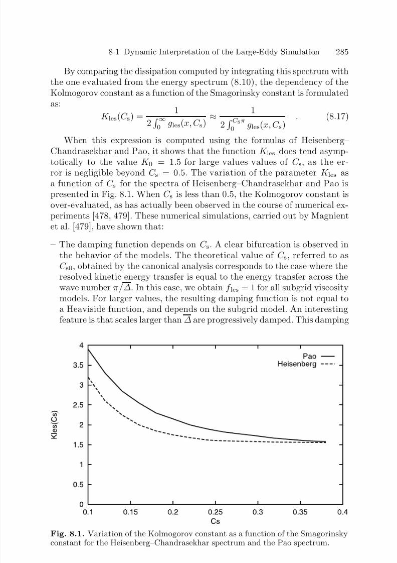
7/21/2019 Large Eddy Simulation for Incompressible Flows
http://slidepdf.com/reader/full/large-eddy-simulation-for-incompressible-flows 306/573
8.1 Dynamic Interpretation of the Large-Eddy Simulation 285
By comparing the dissipation computed by integrating this spectrum withthe one evaluated from the energy spectrum (8.10), the dependency of theKolmogorov constant as a function of the Smagorinsky constant is formulatedas:
K les(C s) = 1
2 ∞
0 gles(x, C s)
≈ 1
2 C sπ
0 gles(x, C s)
. (8.17)
When this expression is computed using the formulas of Heisenberg–Chandrasekhar and Pao, it shows that the function K les does tend asymp-totically to the value K 0 = 1.5 for large values values of C s, as the er-ror is negligible beyond C s = 0.5. The variation of the parameter K les asa function of C s for the spectra of Heisenberg–Chandrasekhar and Pao is
presented in Fig. 8.1. When C s is less than 0.5, the Kolmogorov constant isover-evaluated, as has actually been observed in the course of numerical ex-periments [478, 479]. These numerical simulations, carried out by Magnientet al. [479], have shown that:
– The damping function depends on C s. A clear bifurcation is observed inthe behavior of the models. The theoretical value of C s, referred to asC s0, obtained by the canonical analysis corresponds to the case where theresolved kinetic energy transfer is equal to the energy transfer across thewave number π/∆. In this case, we obtain f les = 1 for all subgrid viscosity
models. For larger values, the resulting damping function is not equal toa Heaviside function, and depends on the subgrid model. An interestingfeature is that scales larger than ∆ are progressively damped. This damping
Fig. 8.1. Variation of the Kolmogorov constant as a function of the Smagorinskyconstant for the Heisenberg–Chandrasekhar spectrum and the Pao spectrum.
7/21/2019 Large Eddy Simulation for Incompressible Flows
http://slidepdf.com/reader/full/large-eddy-simulation-for-incompressible-flows 307/573
286 8. Numerical Solution: Interpretation and Problems
originates from two different phenomena: (i) the energy drain induced bythe subgrid-viscosity model, and (ii) the forward energy cascade, which isresponsible for a net drain of kinetic energy by the modes located withinthe spectral band [(C s/C s0)π/∆, π/∆].
– The damping function is subgrid-model dependent: each subgrid modelleads to a different equilibrium between the two sources of resolved energydrain, yielding different spectra and associated damping functions.
Interpretation of Simulation Parameters.
Effective Filter. The above results allow us to refine the analysis concerningthe effective filter. For large values of the Smagorinsky constant (C s
≥ 0.5),
the characteristic cutoff length is the mixing length produced by the model.The model then dissipates more energy than if it were actually located at thescale ∆ because it ensures the energy flux balance through the cutoff associ-ated with a longer characteristic length. The effective filter is therefore fullydetermined by the subgrid model. This solution criterion should be comparedwith the one defined for hot-wire measurements, which recommends that thewire length be less than twice the Kolmogorov scale in developed turbulentflows.
For small values of the constant, it is the cutoff length ∆ that plays the
role of characteristic length and the effective filter corresponds to the usualanalytical filter. It should be noted in this case that the energy drainageinduced by the model is less than the transfer of kinetic energy through thecutoff, so the energy balance is no longer maintained. This is reflected inan accumulation of energy in the resolved scales, and the pertinence of thesimulation results should be taken with caution.
For intermediate values of the constant, i.e. values close to the theoreticalone predicted in Sect. 5.3.2 (i.e. C s ≈ 0.2), the effective filter is a combinationof the analytical filter and model’s implicit filter, which makes it difficult to
interpret the dynamics of the smallest resolved scales. The dissipation inducedby the model in this case correctly insures the equilibrium of the energy fluxesthrough the cutoff.
Microstructure Knudsen Number. It has already been seen (relation (8.12))that the mixing length can be interpreted as playing a role analogous tothat of the Kolmogorov scale for the direct numerical simulation. The cutoff length ∆, for its part, can be linked to the mean free path for Newtonianfluids. We can use the ratio of these two quantities to define an equivalent of the microstucture Knudsen number K nm for the large-eddy simulation:
K nm = ∆
∆f =
1
C s. (8.18)
Effective Reynolds Number. Let us also note that the effective Reynolds num-ber of the simulation, denoted Reles, which measures the ratio of the inertia

7/21/2019 Large Eddy Simulation for Incompressible Flows
http://slidepdf.com/reader/full/large-eddy-simulation-for-incompressible-flows 308/573
8.1 Dynamic Interpretation of the Large-Eddy Simulation 287
effects to the dissipation effects, is taken in ratio to the Reynolds number Recorresponding to the exact solution by the relation:
Reles = η
ηles
4/3Re , (8.19)
where η is the dissipative scale of the full solution. This decrease in theeffective Reynolds number in the simulation may pose some problems, if thephysical mechanism determining the dynamics of the resolved scales dependsexplicitly on it. This will, for example, be the case for all flows where criticalReynolds numbers can be defined for which bifurcations in the solution areassociated3.
Subfilter Scale Concept. By analysis of the decoupling between the cutoff length of the analytical filter ∆ and the mixing length ∆f , we can definethree families of scales [495, 551] instead of the usual two families of resolvedand subgrid scales. These three categories, illustrated in Fig. 8.2, are the:
1. Subgrid scales, which are those that are excluded from the solution bythe analytical filter.
2. Subfilter scales, which are those of a size less than the effective filter cutoff length, denoted ∆eff , which are scales resolved in the usual sense but
whose dynamics is strongly affected by the subgrid model. Such scalesexist only if the effective filter is determined by the subgrid viscositymodel. There is still the problem of evaluating ∆eff , and depends bothon the presumed shape of the spectrum and on the point beyond which weconsider to be “strongly affected”. For example, by using Pao’s spectrumand defining the non-physically resolved modes as those for which theenergy level is reduced by a factor e = 2.7181..., we get:
∆eff = C sC theo
∆ , (8.20)
where C theo is the theoretical value of the constant that corresponds tothe cutoff length ∆.
3. Physically resolved scales, which are those of a size greater than theeffective filter cutoff length, whose dynamics is perfectly captured by thesimulation, as in the case of direct numerical simulations.
Characterization of the Filter Associated with the Subgrid Model.The above discussion is based on a similarity hypothesis between the prop-
erties of isotropic homogeneous turbulence and those of the flow simulated3 Numerical experiments show that too strong a dissipation induced by the subgrid
model in such flows may inhibit the flow driving mechanisms and consequentlylead to unreliabable simulations. One known example is the use of a Smagorin-sky model to simulate a plane channel flow: the dissipation is strong enough toprevent the transition to turbulence.
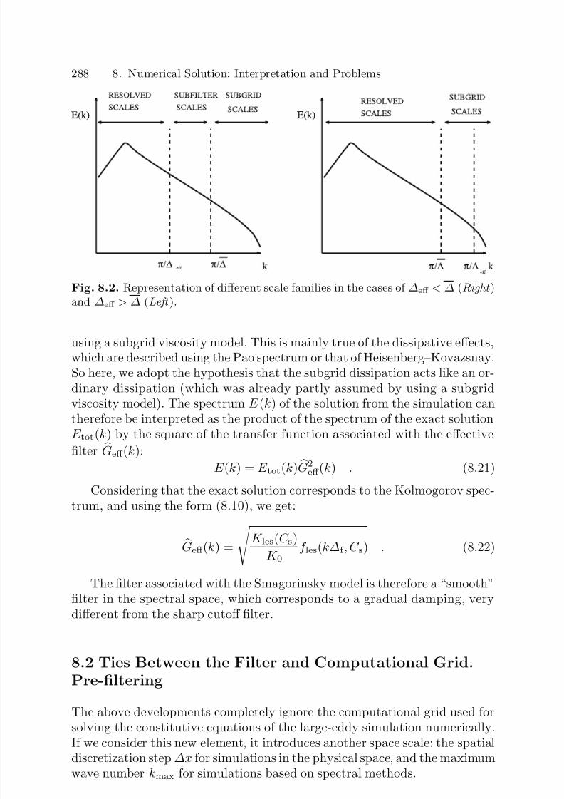
7/21/2019 Large Eddy Simulation for Incompressible Flows
http://slidepdf.com/reader/full/large-eddy-simulation-for-incompressible-flows 309/573
288 8. Numerical Solution: Interpretation and Problems
Fig. 8.2. Representation of different scale families in the cases of ∆eff < ∆ (Right )
and ∆eff > ∆ (Left ).
using a subgrid viscosity model. This is mainly true of the dissipative effects,which are described using the Pao spectrum or that of Heisenberg–Kovazsnay.So here, we adopt the hypothesis that the subgrid dissipation acts like an or-dinary dissipation (which was already partly assumed by using a subgridviscosity model). The spectrum E (k) of the solution from the simulation can
therefore be interpreted as the product of the spectrum of the exact solutionE tot(k) by the square of the transfer function associated with the effective
filter Geff (k):
E (k) = E tot(k) G2eff (k) . (8.21)
Considering that the exact solution corresponds to the Kolmogorov spec-trum, and using the form (8.10), we get:
Geff (k) = K les(C s)
K 0
f les(k∆f , C s) . (8.22)
The filter associated with the Smagorinsky model is therefore a “smooth”filter in the spectral space, which corresponds to a gradual damping, verydifferent from the sharp cutoff filter.
8.2 Ties Between the Filter and Computational Grid.
Pre-filtering
The above developments completely ignore the computational grid used forsolving the constitutive equations of the large-eddy simulation numerically.If we consider this new element, it introduces another space scale: the spatialdiscretization step ∆x for simulations in the physical space, and the maximumwave number kmax for simulations based on spectral methods.

7/21/2019 Large Eddy Simulation for Incompressible Flows
http://slidepdf.com/reader/full/large-eddy-simulation-for-incompressible-flows 310/573
8.2 Ties Between the Filter and Computational Grid. Pre-filtering 289
The discretization step has to be small enough to be able to correctlyintegrate the convolution product that defines the analytical filtering. Forfilters with fastly-decaying kernel, we have the relation:
∆x ≤ ∆ . (8.23)
The case where ∆x = ∆ is the optimal case as concerns the number of de-grees of freedom needed in the discrete system for performing the simulation.This case is illustrated in Fig. 8.3.
Fig. 8.3. Representation of spectral decompositions associated with pre-filtering(Left ) and in the optimal case (Right ).
The numerical errors stemming from the resolution of the discretized sys-tem still have to be evaluated. To ensure the quality of the results, the numer-ical error committed on the physically resolved modes has to be negligible,and therefore committed only on the subfilter scales. The theoretical analysis
of this error by Ghosal in the simple case of isotropic homogeneous turbulenceis presented in the following.As the numerical schemes used are consistent, the discretization error can-
cels out as the space and time steps tend toward zero. One way of minimizingthe effect of numerical error is to reduce the grid spacing while maintainingthe filter cutoff length, which comes down to increasing the ratio ∆/∆x (seeFig. 8.3). This technique, based on the decoupling of the two space scales, iscalled pre-filtering [14], and aims to ensure the convergence of the solutionregardless of the grid4. It minimizes the numerical error but induces morecomputations because it increases the number of degree of freedoms in thenumerical solution without increasing the number of degrees of freedom inthe physically resolved solution, and requires that the analytical filtering be
4 A simplified analysis shows that, for an nth-order accurate numerical method,the weight of the numerical error theoretically decreases as (∆/∆x)−n. A finerestimate is given in the remainder of this chapter.

7/21/2019 Large Eddy Simulation for Incompressible Flows
http://slidepdf.com/reader/full/large-eddy-simulation-for-incompressible-flows 311/573
290 8. Numerical Solution: Interpretation and Problems
performed explicitly [14] [59]. Because of its cost5, this solution is rarely usedin practice.
Another approach is to link the analytical filter to the computed grid. Theanalytical cutoff length is associated with the space step using the optimalratio of these quantities and the form of the convolution kernel is associatedwith the numerical method. Let us point out a problem here that is analogousto that of the effective filter already mentioned: the effective numerical filterand therefore the effective numerical cutoff length, are generally unknown.This method has the advantage of reducing the size of the system as bestpossible and not requiring the use of an analytical filter, but it allows noexplicit control of the effective numerical filter, which makes it difficult tocalibrate the subgrid models. This method, because of its simplicity, is used
by nearly all the authors.
8.3 Numerical Errors and Subgrid Terms
8.3.1 Ghosal’s General Analysis
Ghosal [259] proposes a non-linear analysis of the numerical error in the solu-tion of the Navier–Stokes equations for an isotropic homogeneous turbulent
flow whose energy spectrum is approximated by the Von Karman model.
Classification of Different Sources of Error. In order to analyze andestimate the discretization error, we first need a precise definition of it. In allof the following, we consider a uniform Cartesian grid of N 3 points, whichare the degrees of freedom of the numerical solution. Periodicity conditionsare used on the domain boundaries.
A first source of error stems from the approximation we make of a contin-uous solution u by a making a discrete solution ud with a set of N 3 values.This is evaluated as:
|ud − P (u)| , (8.24)
where P is a definite projection operator of the space of continuous solu-tions to that of the discrete solutions. This error is minimum (in the L2
sense) if P is associated with the decomposition of the continuous solutionon a finite base of trigonometric polynomials, with the components of ud
being the associated Fourier coefficients. This error is intrinsic and cannot becanceled. Consequently, it will not enter into the definition of the numerical
5 For a fixed value of ∆, increasing the ratio ∆/∆x by a factor n leads to anincrease in the number of points of the simulation by a factor of n3 and increasesthe number of time steps by a factor n in order to maintain the same ratiobetween the time and space steps. In all, this makes an overall increase in thecost of the simulation by a factor n4.
7/21/2019 Large Eddy Simulation for Incompressible Flows
http://slidepdf.com/reader/full/large-eddy-simulation-for-incompressible-flows 312/573
8.3 Numerical Errors and Subgrid Terms 291
error discussed in this present section. The best possible discrete solution isuopt ≡ P (u).
The equations of the continuous problem are written in the symbolic form:
∂ u
∂t = NS (u) , (8.25)
where NS is the Navier–Stokes operator. The optimal discrete solution uopt
is a solution of the problem:
∂ P u∂t
= P N S (u) , (8.26)
where P NS is the optimal discrete Navier–Stokes operator which, in thefixed framework, corresponds to the discrete operators obtained by a spectralmethod.
Also, we note the discrete problem associated with a fixed discrete schemeas:
∂ ud
∂t = NS d(ud) . (8.27)
By taking the difference between (8.26) and (8.27), it appears that thebest possible numerical method, denoted NS opt, is the one that verifies the
relation: NS opt P = P N S . (8.28)
The numerical error E num associated with the NS d scheme, and which isanalyzed in the following, is defined as:
E num ≡ (P N S − N S d P ) (u) . (8.29)
This represents the discrepancy between the numerical solution and theoptimal discrete one. To simplify the analysis, we consider in the following
that the subgrid models are perfect, i.e. that they induce no error with respectto the exact solution of the filtered problem. By assuming this, we can clearlyseparate the numerical errors from the modeling errors.
The numerical error E num(k) associated with the wave number k is de-composed as the sum of two terms of distinct origins:
– The differentiation error E df (k), which measures the error the discrete op-erators make in evaluating the derivatives of the wave associated with k.Let us note that this error is null for a spectral method if the cutoff fre-quency of the numerical approximation is high enough.
– The spectrum aliasing error E rs(k), which is due to the fact that we arecomputing non-linear terms in the physical space in a discrete space of finitedimension. For example, a quadratic term will bring in higher frequenciesthan those of each of the arguments in the product. While some of thesefrequencies are too high to be represented directly on the discrete base,
7/21/2019 Large Eddy Simulation for Incompressible Flows
http://slidepdf.com/reader/full/large-eddy-simulation-for-incompressible-flows 313/573
292 8. Numerical Solution: Interpretation and Problems
they do combine with the low frequencies and introduce an error in therepresentation of them6.
Estimations of the Error Terms. For a solution whose spectrum is of theform proposed by Von Karman:
E (k) = a k4
(b + k2)17/6 , (8.30)
with a = 2.682 and b = 0.417, and using a quasi-normality hypothesis forevaluating certain non-linear terms, Ghosal proposes a quantitative evalua-tion of the different error terms, the subgrid terms, and the convection term,
for various Finite Difference schemes as well as for a spectral scheme. Theconvection term is written in conservative form and all the schemes in spaceare centered. The time integration is assumed to be exact.
The exact forms of these terms, available in the original reference work,are not reproduced here. For a cutoff wave number kc and a sharp cutoff filter,simplified approximate estimates of the average amplitude can be derived forsome of these terms.
The amplitude of the subgrid term σsgs(kc), defined as
σsgs(kc) = kc
0
|τ (k)|dk1/2
, (8.31)
where τ (k) is the subgrid term for the wave number k, is bounded by:
σsgs(kc) =
0.36 k0.39
c upper limit0.62 k0.48
c lower limit , (8.32)
that of the sum of the convection term and subgrid term by:
σtot(kc) = 1.04 k0.97c , (8.33)
6 Let us take the Fourier expansions of two discrete functions u and v representedby N degrees of freedom. At the point of subscript j, the expansions are ex-pressed:
uj =
N/2−1n=−N/2
une(i(2π/N )jn), vj =
N/2−1m=−N/2
vme(i(2π/N )jm) j = 1, N .
The Fourier coefficient of the product wj = ujvj (without summing on j) splits
into the form:wk =
n+m=k
un vm +
n+m=k±N
un vm .
The last term in the right-hand side represents the spectrum aliasing error. Theseare terms of frequencies higher than the Nyquist frequency, associated the sam-pling, which will generate spurious resolved frequencies.
7/21/2019 Large Eddy Simulation for Incompressible Flows
http://slidepdf.com/reader/full/large-eddy-simulation-for-incompressible-flows 314/573
8.3 Numerical Errors and Subgrid Terms 293
in whichσsgs(kc)
σtot(kc) ≈ k−0.5
c . (8.34)
The amplitude of the differentiation error σdf (kc), defined by:
σdf (kc) =
kc
0
E df (k)dk
1/2
, (8.35)
is evaluated as:
σdf (kc) = k0.75
c ×
1.03 (second order)0.82 (fourth order)0.70 (sixth order)0.5 (heigth order)0 (spectral)
, (8.36)
and the spectrum aliasing error σrs(kc), which is equal to:
σrs(kc) =
kc
0
E rs(k)dk
1/2
(8.37)
is estimated as:
σrs =
0.90 k0.46c (minimum estimation, spectral, no de-aliasing)2.20 k0.66
c (maximum estimation, spectral, no de-aliasing)0.46 k0.41
c (minimum estimation, second order)1.29 k0.65
c (maximum estimation, second order)
.
(8.38)The spectrum aliasing error for the spectral method can be reduced to
zero by using the 2/3 rule, which consists of not considering the last thirdof the wave numbers represented by the discrete solution. It should be notedthat, in this case, only the first two-thirds of the modes of the solution are
correctly represented numerically. The error of the finite difference schemesof higher order is intermediate between that of the second-order accuratescheme and that of the spectral scheme.
From these estimations, we can see that the discretization error domi-nates the subgrid terms for all the finite difference schemes considered. Thesame is true for the spectrum aliasing error, including for the finite differ-ence schemes. Finer analysis on the basis of the spectra of the various termsshows that the discretization error is dominant for all wave numbers for thesecond-order accurate scheme, whereas the subgrid terms are dominant at
the low frequencies for the heigth-order accurate scheme. In the former case,the effective numerical filter is dominant and governs the solution dynamics.Its cutoff length can be considered as being of the order of the size of thecomputational domain. In the latter, its cutoff length, defined as the wave-length of the mode beyond which it becomes dominant with respect to thesubgrid terms, is smaller and there exist numerically well-resolved scales.

7/21/2019 Large Eddy Simulation for Incompressible Flows
http://slidepdf.com/reader/full/large-eddy-simulation-for-incompressible-flows 315/573
294 8. Numerical Solution: Interpretation and Problems
8.3.2 Pre-filtering Effect
The pre-filtering effect is clearly visible from relations (8.32) to (8.38). By
decoupling the analytical from the numerical filter, two different cutoff scalesare introduced and thereby two different wave numbers for evaluating thenumerical error terms and the subgrid terms: while the cutoff scale ∆ associ-ated with the filter remains constant, the scale associated with the numericalerror (i.e. ∆x) is now variable.
By designating the ratio of the two cutoff lengths by C rap = ∆x/∆ < 1,we see that the differentiation error σdf (kc) of the finite difference scheme is
reduced by a factor C −3/4rap with respect to the previous case, since it varies
as k3/4c . This reduction is much greater than the one obtained by increasing
the order of accuracy of the the schemes.Thus, more detailed analysis shows that, for the second-order accurate
scheme, the dominance of the subgrid term on the whole of the solutionspectrum is ensured for C rap = 1/8. For a ratio of 1/2, this dominance isonce again found for schemes of order of accuracy of 4 or more.
These theoretical evaluations do not take into account the nonlinear feed-back of the computed solution on the numerical error. Numerical experimentswere conducted by Chow and Moin [138] in isotropic turbulence to assessGhosal’s results. Their results show that to ensure that the subgrid terms
will dominate the numerical error, a filter-grid ratio ∆/∆x of at least four isdesired for a second-order centered finite difference scheme. This minimumis a decreasing function of the scheme order of accuracy, and a ratio of twois found to be sufficient for a sixth-order centered Pade scheme.
The efficiency of the prefiltering technique was exhaustively checked byGeurts and Frohlich [256, 257] on the plane mixing layer configuration. Themain conclusion of this study is that the best solution for improving the re-sults of a large-eddy simulation in practice is to refine the computational grid,i.e. to lower ∆x, while keeping a low value of the ratio ∆/∆x. The numerical
tests conducted by these authors show that ∆/∆x = 1 is optimal for high-resolution large-eddy simulations, i.e. for simulations which are close to directnumerical simulation. For coarser grid simulation, the optimum was found tobe ∆/∆x ≈ 2 − 3, combined with a fourth-order accurate non-dissipativenumerical method. Nevertheless, the recommended strategy to improve theresults at a fixed computational cost is to refine the grid using ∆/∆x = 1−2rather than augmenting the ratio ∆/∆x for a given value of ∆. This con-clusion is confirmed by a large set of results published by Gullbrand andChow [283], who carried out several simulations of turbulent plane channel
flow with second-order and fourth-order accurate finite difference methods.In these simulations, the use of a prefilter with size 2∆x didn’t lead to a clearimprovement of the results.
The finest study of the effect of prefiltering was conducted by Meyers,Geurts and Baelmans [515] in large-eddy simulation of isotropic turbulenceusing the Smagorinsky model. Defining the error etotal(∆,∆x) for a dummy
7/21/2019 Large Eddy Simulation for Incompressible Flows
http://slidepdf.com/reader/full/large-eddy-simulation-for-incompressible-flows 316/573
8.3 Numerical Errors and Subgrid Terms 295
variable φ as the difference between the filtered exact solution (obtainedby Direct Numerical Simulation) and the solution found using large-eddysimulation with cutoff length ∆ on a mesh of size ∆x:
etotal(∆,∆x) = φDNS − φLES(∆,∆x) , (8.39)
the authors investigate the relative influence of different sources of error.Subgrid modeling and discretization errors being respectively defined as
emodel = φDNS − φLES(∆, 0) , (8.40)
ediscr = φLES(∆, 0) − φLES(∆,∆x) , (8.41)
exhaustive analyses carried out using a direct numerical simulation databaseyields the following conclusions:
– The global error behavior is parametrized by the subgrid activity parame-ter s defined like
s = ε
ε + εν , (8.42)
where ε = −τ ijS ij is the subgrid dissipation and εν = νS ijS ij is themolecular dissipation. Direct numerical simulation corresponds to s = 0,while s = 1 characterizes large-eddy simulation in the limit of infiniteReynolds number. Tests prove there there exists a threshold value sc7: fors ≤ sc the total error is dominated by discretization error effects, while fors > sc the modeling error is the most important source of uncertainty.
– For s ≤ sc, the relative error δ err:
δ err =
e2
totaldt φDNS
2dt
, (8.43)
can be either a decreasing or increasing function of s, depending on s and
∆x when it is based on the kinetic energy (see Fig. 8.4). No general trendis observed in this regime, in which strong interactions can occur betweendiscretization errors and modeling errors. Partial cancellation sometimesoccurs leading to a significant reduction of the total error. For s > sc, therelative error is a monotone exponentially increasing function of s.
– The relative error based on the Taylor length scale has a different behaviorin the s ≤ sc regime (see Fig. 8.5): strong interactions between model-ing and discretization errors are observed, but the relative error exhibitsa monotonic increasing behavior as a function of sc. Partial error cancel-
lation is less intense than in the case of the turbulent kinetic energy.– Because of the strong non-linear interactions between modeling and dis-
cretization errors, which leads to a non-monotone behavior of the total
7 Typical values are sc = 0.4 for isotropic turbulence at Reλ = 50, sc = 0.8 forisotropic turbulence at Reλ = 100 and sc = 0.5 for a plane mixing layer.

7/21/2019 Large Eddy Simulation for Incompressible Flows
http://slidepdf.com/reader/full/large-eddy-simulation-for-incompressible-flows 317/573
296 8. Numerical Solution: Interpretation and Problems
Fig. 8.4. Evolution of the relative error on kinetic energy as a function of thesubgrid activity, in isotropic turbulence (Courtesy of J. Meyers and B. Geurts,Univ. Twente). Top: Reλ = 50, Bottom: Reλ = 100.

7/21/2019 Large Eddy Simulation for Incompressible Flows
http://slidepdf.com/reader/full/large-eddy-simulation-for-incompressible-flows 318/573
8.3 Numerical Errors and Subgrid Terms 297
Fig. 8.5. Evolution of the relative error on the Taylor scale as a function of thesubgrid activity, in isotropic turbulence (Courtesy of J. Meyers and B. Geurts, Univ.
Twente). Left: Reλ = 50, Right: Reλ = 100.
error. As a consequence, grid refinement (decrease of ∆x at constant ∆)must be coupled to a change in the Smagorinsky constant C S to obtainan optimal error minimization. The ratio C S ∆/∆x which yields the mini-mum error follows non-trivial trajectories in both the (∆x,C S ∆) and the(∆x, s/sc) planes. This behavior is illustrated in Fig. 8.6.
8.3.3 Conclusions
This analysis can be used only for reference, because it is based on veryrestrictive hypotheses. It nonetheless indicates that the numerical error isnot negligible and that it can even be dominant in certain cases over thesubgrid terms. The effective numerical filter is then dominant over the scaleseparation filter.
This error can be reduced either by increasing the order of accuracy of the numerical scheme or by using a pre-filtering technique that decouples
the cutoff length of the analytical filter of the discretization step. Ghosal’sfindings seem to indicate that a combination of these two techniques wouldbe the most effective solution.
These theoretical findings are confirmed by the numerical experimentsof Najjar and Tafti [563] and Kravenchko and Moin [409], who observedthat the effect of the subgrid models is completely or partially masked bythe numerical error when second-order accurate methods are employed. Itshould be noted here that practical experience leads us to less pessimisticconclusions than the theoretical analyses: large-eddy simulations performed
with a scheme accurate to the second order show a dependency with respect tothe subgrid model used. The effects of these models are not entirely masked,which justifies using them. However, no precise qualification exists today of the information loss due to the use of a given scheme. These observations aremade empirically, case by case [76, 480, 94].
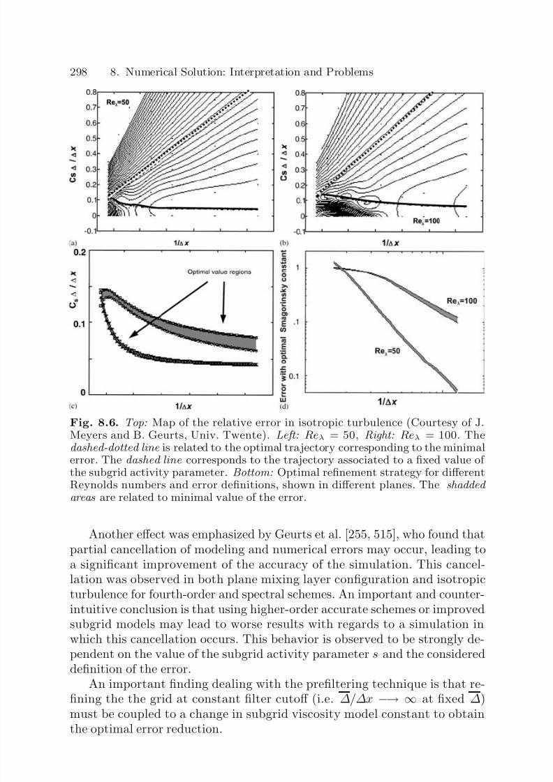
7/21/2019 Large Eddy Simulation for Incompressible Flows
http://slidepdf.com/reader/full/large-eddy-simulation-for-incompressible-flows 319/573
298 8. Numerical Solution: Interpretation and Problems
Fig. 8.6. Top: Map of the relative error in isotropic turbulence (Courtesy of J.Meyers and B. Geurts, Univ. Twente). Left: Reλ = 50, Right: Reλ = 100. Thedashed-dotted line is related to the optimal trajectory corresponding to the minimalerror. The dashed line corresponds to the trajectory associated to a fixed value of the subgrid activity parameter. Bottom: Optimal refinement strategy for differentReynolds numbers and error definitions, shown in different planes. The shadded areas are related to minimal value of the error.
Another effect was emphasized by Geurts et al. [255, 515], who found that
partial cancellation of modeling and numerical errors may occur, leading toa significant improvement of the accuracy of the simulation. This cancel-lation was observed in both plane mixing layer configuration and isotropicturbulence for fourth-order and spectral schemes. An important and counter-intuitive conclusion is that using higher-order accurate schemes or improvedsubgrid models may lead to worse results with regards to a simulation inwhich this cancellation occurs. This behavior is observed to be strongly de-pendent on the value of the subgrid activity parameter s and the considereddefinition of the error.
An important finding dealing with the prefiltering technique is that re-fining the the grid at constant filter cutoff (i.e. ∆/∆x −→ ∞ at fixed ∆)must be coupled to a change in subgrid viscosity model constant to obtainthe optimal error reduction.
7/21/2019 Large Eddy Simulation for Incompressible Flows
http://slidepdf.com/reader/full/large-eddy-simulation-for-incompressible-flows 320/573
8.3 Numerical Errors and Subgrid Terms 299
8.3.4 Remarks on the Use of Artificial Dissipations
Many comments have been made over recent decades on the sensitivity of
large-eddy simulation results, for example concerning the formulation of theconvection term [319, 409], the discrete form of the test filter [597, 563, 81,641, 605], and the formulation of the subgrid term [634], but there are far toomany, too dispersed, and too far from general to be detailed here. Moreover,countless analyses have been made of the numerical error associated withvarious schemes, especially as concerns the treatment of the non-linear terms,which will not be resumed here, but we will still take more special note of the findings of Fabignon et al. [211] concerning the characterization of theeffective numerical filter of several schemes.
Special attention should still be paid to the discretization of the convec-tive terms. To capture strong gradients without having the numerical solutionpolluted with spurious high-frequency wiggles, the scheme is very often stabi-lized by introducing artificial dissipation. This dissipation is added explicitlyor implicitly using an upwind scheme for the convection term. Introducingan additional dissipation term for the large-eddy simulation is still controver-sial [563, 521, 239, 228, 665, 501, 94] because the effective filter is then verysimilar in form to that which would be imposed by subgrid viscosity model,making for two competing resolved kinetic energy spectrum mechanisms. The
similarity between the numerical dissipation and that associated with the en-ergy cascade model is still being investigated, but a few conclusions havealready been drawn.
It seems that the total numerical dissipation induced by most upwindschemes is still greater than that of the subgrid viscosity models, if no pre-filtering method is used. This is true even for seventh-order accurate upwindschemes [52].
Garnier et al. [239] developed the generalized Smagorinsky constant asa tool to compare numerical and physical subgrid dissipations. The general-
ized Smagorinsky constant is the value that should take the constant of theSmagorinsky model to obtain a total dissipation equal to the numerical dis-sipation. Numerical tests carried out on decaying isotropic turbulence haveshown that all the numerical upwind schemes, up to the fifth order of accu-racy, are more dissipative than the usual Smagorinsky model. Typical resultsare displayed in Fig. 8.7.
It has also been demonstrated [501] that the use of a stabilized sixth-orderaccurate scheme may lead to the same quality of results as a second-orderaccurate scheme, because of the very high dissipation applied to the highest
resolved frequency, which is responsible for the largest part of the interactionswith subgrid modes. These two dissipations are correlated in space (especiallyin the case of the Smagorinsky model), but have different spectral distribu-tions: a subgrid viscosity model corresponds to a second-order dissipationassociated with a spectrum of the form (k/kc)2E (k), while an nth-order nu-merical dissipation is associated with a spectrum of the form (k/kc)nE (k).

7/21/2019 Large Eddy Simulation for Incompressible Flows
http://slidepdf.com/reader/full/large-eddy-simulation-for-incompressible-flows 321/573
300 8. Numerical Solution: Interpretation and Problems
Fig. 8.7. Time history of the generalized Smagorinsky constant for various dis-sipative schemes (second- to fifth-order of accuracy) in freely decaying isotropicturbulence. Courtesy of E. Garnier, ONERA.
For n > 2 (resp. n < 2), the numerical (resp. subgrid) dissipation may be
dominant for the highest resolved frequencies and the subgrid (resp. numer-ical) dissipation will govern the dynamics of the low frequencies. This pointis illustrated in Figs. 8.8 and 8.9.
Fig. 8.8. Numerical and subgrid dissipations for a Von Karman spectrum. Thepeak of the Von Karman spectrum is at kc/5. The dissipation spectra have beennormalized so that the total dissipation is the same in all cases. It is worth notingthat typical numerical schemes lead to a total dissipation higher than the subgriddissipation.
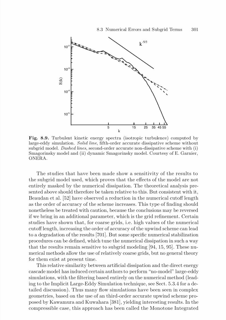
7/21/2019 Large Eddy Simulation for Incompressible Flows
http://slidepdf.com/reader/full/large-eddy-simulation-for-incompressible-flows 322/573
8.3 Numerical Errors and Subgrid Terms 301
Fig. 8.9. Turbulent kinetic energy spectra (isotropic turbulence) computed bylarge-eddy simulation. Solid line , fifth-order accurate dissipative scheme withoutsubgrid model. Dashed lines , second-order accurate non-dissipative scheme with (i)Smagorinsky model and (ii) dynamic Smagorinsky model. Courtesy of E. Garnier,ONERA.
The studies that have been made show a sensitivity of the results tothe subgrid model used, which proves that the effects of the model are notentirely masked by the numerical dissipation. The theoretical analysis pre-sented above should therefore be taken relative to this. But consistent with it,Beaudan et al. [52] have observed a reduction in the numerical cutoff lengthas the order of accuracy of the scheme increases. This type of finding shouldnonetheless be treated with caution, because the conclusions may be reversedif we bring in an additional parameter, which is the grid refinement. Certain
studies have shown that, for coarse grids, i.e. high values of the numericalcutoff length, increasing the order of accuracy of the upwind scheme can leadto a degradation of the results [701]. But some specific numerical stabilizationprocedures can be defined, which tune the numerical dissipation in such a waythat the results remain sensitive to subgrid modeling [94, 15, 95]. These nu-merical methods allow the use of relatively coarse grids, but no general theoryfor them exist at present time.
This relative similarity between artificial dissipation and the direct energycascade model has induced certain authors to perform “no-model” large-eddysimulations, with the filtering based entirely on the numerical method (lead-ing to the Implicit Large-Eddy Simulation technique, see Sect. 5.3.4 for a de-tailed discussion). Thus many flow simulations have been seen in complexgeometries, based on the use of an third-order accurate upwind scheme pro-posed by Kawamura and Kuwahara [381], yielding interesting results. In thecompressible case, this approach has been called the Monotone Integrated

7/21/2019 Large Eddy Simulation for Incompressible Flows
http://slidepdf.com/reader/full/large-eddy-simulation-for-incompressible-flows 323/573
302 8. Numerical Solution: Interpretation and Problems
Large-Eddy Simulation (MILES) method (see Sect. 5.3.4 for a description of ILES numerical methods). The “experimental” analysis of some particularnumerical methods reveals that there exists some numerical dissipation pro-cedures which mimic very well the theoretical subgrid viscosity [192]. Thisis illustrated in Fig. 8.10, which compares the computes spectral viscosityassociated to the MPDATA scheme with the theoretical spectral viscosityprofile. The observed agreement prove that the Implict Large-Eddy Simula-tion approach can yield very good results if the numerical scheme is carefullychosen.
The use of artificial dissipation therefore raises many questions, but isvery common in simulations that are physically very strongly under-resolvedin complex configurations, because experience shows that adding subgrid
models does not ensure a monotonic solution. To ensure that certain variablesremain positive, such as concentrations of pollutants or the temperature, itseems to be necessary to resort to such numerical methods. Alternatives basedon local refinement of the solution, i.e. decreasing the effective cutoff lengthby enriching or adapting the grid, have been studied by certain authors butno final conclusion has been drawn.
A few studies dealing with some particular stabilization techniques suchas the Galerkin Least-Square method, reveal that the numerical dissipationmay happen to be be too low to prevent a pile-up in the resolved kinetic
energy, leading to the growth of bounded wiggles. In such a case, the use of a subgrid model seems to be required to recoved physical results. The mainproblem arising in this case is that the use of a basic subgrid model will leadto a global overdamping of the computed solution. The use of self-adaptivesubgrid models able to tune their induced dissipation so that the sum of
Fig. 8.10. Analysis of the numerical viscosity associated to the MPDATA scheme.Dashed line: theoretical spectral subgrid viscosity. Solid line: MPDATA equiva-lent spectralk viscosity. Solid line with symbol: spectral viscosity recomputed fromkinetic energy transfer of the unfiltered velocity field. From [192].
7/21/2019 Large Eddy Simulation for Incompressible Flows
http://slidepdf.com/reader/full/large-eddy-simulation-for-incompressible-flows 324/573
8.3 Numerical Errors and Subgrid Terms 303
the numerical and subgrid dissipation will reach the required level to obtainphysical results. The identification of subgrid models and/or procedures todefine such subgrid models is still a open issue. An a priori requirement isthat the subgrid model must be local in terms of wave number, i.e. it mustemphasized the highest resolved frequencies. Numerical experiments showthat self-adaptive models and some multilevel approaches have this property.
While the Navier–Stokes equations contain energy information, they alsocontain information concerning the signal phase. Using centered schemes forthe convection term therefore raises problems too, because of the dispersiveerrors they induce in the highest resolved frequencies.
Generally, estimates of the wave number beyond which the modes areconsidered to be well resolved numerically vary from 2∆x to 20∆x, depending
on the schemes and authors [604].
8.3.5 Remarks Concerning the Time Integration Method
Large-eddy simulation is ordinarily addressed using a spatial filtering, butwithout explicitly stating the associated time filtering. This is due to the factthat most computations are made for moderate time steps (CFL ≡ u∆t/∆x < 1) and it is felt that the time filtering effects are masked by those of the space filtering. Choi and Moin [131], however, have shown by direct simu-lations of a plane channel flow that the time filtering effects can be very large,even for CFLs of the order of 0.5, since the turbulence cannot be maintainednumerically if the time step is greater than the characteristic time associatedwith the Kolmogorov scale. Most authors use second-order accurate integra-tion methods, but no complete study has been published to date to determinewhat timescales are well resolved numerically and physically. We should alsonote the results of Beaudan and Moin [52] and Mittal and Moin [521], whoshowed that the use of artificial viscosity affects the solution of a very largeshare of the simulated time frequencies (about 75% for the particular case
studied).
7/21/2019 Large Eddy Simulation for Incompressible Flows
http://slidepdf.com/reader/full/large-eddy-simulation-for-incompressible-flows 325/573
9. Analysis and Validationof Large-Eddy Simulation Data
9.1 Statement of the Problem
9.1.1 Type of Information Contained in a Large-Eddy Simulation
The solution to the equations that define the large-eddy simulation furnishesexplicit information only on the scales that are resolved, i.e. those that areleft after reduction of the number of degrees of freedom in the exact solution.We are therefore dealing with information that is truncated in space andtime. The time filtering is induced implicitly by the spatial filtering because,as the filtering eliminates certain space scales, it eliminates the correspondingtime scales with them (see p. 19).
The information of use for analysis or validation is what is contained inthose scales that are both physically and numerically well-resolved. It shouldbe remembered that, since the effective numerical and physical filters areunknown, the usable scales are most often identified empirically.
Adopting the assumption that all the scales represented by the simula-tion are physically and numerically well-resolved, the statistical average of the usable resolved field is expressed u. The statistical fluctuation of theresolved field, denoted u, is defined by:
ui = ui−
ui
. (9.1)
The difference between the statistical average of the resolved scales andthat of the exact solution is defined as:
ui − ui = ui , (9.2)
which corresponds to the statistical average of the unresolved scales. TheReynolds stresses computed from the resolved scales are equal to ui u
j .
The difference from the exact stresses uei uej , where the exact fluctuation is
defined as ue = u
− u
, is:
uei uej = (ui − ui)(uj − uj)
= uiuj − uiuj= uiuj + τ ij − ui + uiuj + uj

7/21/2019 Large Eddy Simulation for Incompressible Flows
http://slidepdf.com/reader/full/large-eddy-simulation-for-incompressible-flows 326/573
306 9. Analysis and Validation
= uiuj + τ ij − uiuj − uiuj − uiuj − uiuj= ui u
j + τ ij − uiuj − uiuj − uiuj ,
where τ ij = uiuj + ujui + uiuj is the defiltered subgrid tensor.Since the subgrid scales are not known, the terms containing the contri-
bution u, cannot be computed from the simulation. When the statisticalaverage of the subgrid modes is very small compared with the other terms,we get:
uei uej ui u
j + τ ij . (9.3)
The two terms on the right-hand side can be evaluated from the numericalsimulation, but the quality of the model’s representation of the subgrid tensorpartly conditions that of the result. We can easily see that subgrid-viscositymodels, which only account for the deviatoric part of the subgrid-stress ten-sor, make it possible only to recover the deviatoric part of the Reynoldsstresses [760, 397], at least theoretically.
9.1.2 Validation Methods
The subgrid models and their various underlying hypotheses can be validatedin two ways [218]:
– A priori validation. The exact solution, which is known in this case, isfiltered analytically, leading to the definition of a fully determined re-solved field and subgrid field. The various hypotheses or models can thenbe tested. The exact solutions are usually generated by direct numericalsimulations at moderate or low Reynolds numbers, which limits the field of investigation. A priori tests like this have also been performed using exper-imental data, making it possible to reach higher Reynolds numbers. Thistype of validation raises a fundamental problem, though. By comparingthe exact subgrid stresses with those predicted by a subgrid model evalu-ated on the basis of the filtered exact solution, the effects of the modelingerrors are neglected and the implicit filter associated with the model is notconsidered1. This means that the results of a priori validations are onlyrelative in value.
– A posteriori validation. Here, we perform a large-eddy simulation compu-tation and validate by comparing its results with a reference solution. Thisis a dynamic validation that takes all the simulation factors into consid-eration, while the previous method is static. Experience shows that mod-els yielding poor a priori results can be satisfactory a posteriori , and vice
1
This field could not have been obtained by a large-eddy simulation since it isa solution of the filtered momentum equations in which the exact subgrid tensorappears. In the course of a simulation, the subgrid model is applied to a velocityfield that is a solution of the momentum equation where the modeled subgridtensor appears. These two fields are therefore different in theory. Consequently,in order to be fully representative, an a priori test has to be performed on thebasis of a velocity field that can be obtained from the subgrid model studied.

7/21/2019 Large Eddy Simulation for Incompressible Flows
http://slidepdf.com/reader/full/large-eddy-simulation-for-incompressible-flows 327/573
9.1 Statement of the Problem 307
versa [597]. It is more advantageous to validate models a posteriori becauseit corresponds to their use in the simulation; but it is sometimes difficult todraw any conclusions on a precise point because of the multitude of oftenimperfectly controlled factors at play in a numerical simulation.
9.1.3 Statistical Equivalency Classes of Realizations
The subgrid models are statistical models and it seems pointless to expectthem to produce deterministic simulations in which the resolved scales coin-cide exactly with those of other realizations, for example of the experimentalsort. On the other hand, large-eddy simulation should correctly reproducethe statistical behavior of the scales making up the resolved field. Equiva-lency classes can thus be defined among the realizations [503] by consideringthat one of the classes consists of realizations that lead to the same values of certain statistical quantities computed from the resolved scales.
Belonging to the same class of equivalency as a reference solution is a vali-dation criterion for the other realizations. If we set aside the numerical errors,we can define the necessary conditions on the subgrid models such that tworealizations will be equivalent, by verifying these validity criteria. These con-ditions will be discussed in the following sections. A subgrid model can thusbe considered validated if it can generate realizations that are equivalent toa reference solution, in a sense defined below.
Theoretically, while we overlook the effect of the discretization on themodeling, it can be justifiably thought that a model reproducing the inter-scale interactions exactly will produce good results, whereas the oppositeproposition is not true. That is, the idea of sufficient complexity of a modelhas to be introduced in order to obtain a type of result on a given configu-ration with a tolerated margin of error in order to say what a good modelis. The idea of a universal or best model might not be rejected outright,but should be taken relatively. The question is thus raised of knowing what
statistical properties two subgrid models should share in order for the tworesulting solutions to have common properties.
Let u and u∗ be the filtered exact solution and the solution computedwith a subgrid model, respectively, for the same filter. The exact (unmodeled)subgrid tensor corresponding to u is denoted τ ij, and the modeled subgridtensor computed from the u∗ field is denoted τ ∗ij(u∗). The two velocity fieldsare solutions of the following momentum equations:
∂ u
∂t
+
∇ ·(u
⊗u) =
−∇ · p + ν
∇2u
− ∇ ·τ , (9.4)
∂ u∗
∂t + ∇ · (u∗ ⊗ u∗) = −∇ · p∗ + ν ∇2u∗ − ∇ · τ ∗(u∗) . (9.5)
A simple analysis shows that, if all the statistical moments (at all pointsof space and time) of τ ij conditioned by the u field are equal to those of

7/21/2019 Large Eddy Simulation for Incompressible Flows
http://slidepdf.com/reader/full/large-eddy-simulation-for-incompressible-flows 328/573
308 9. Analysis and Validation
τ ∗ij(u∗) conditioned by u∗, then all the statistical moments of u and u∗
will be equal. This is a full statistical equivalency, which implies that thesubgrid models fulfill an infinity of conditions. To relax this constraint, wedefine less restrictive equivalency classes of solutions which are describedin the following sections. They are defined in such a way as to bring outthe necessary conditions applying to the subgrid models, in order to qualifythem [503]. We try to define conditions such that the statistical moments of moderate order2 (1 and 2) of the field resulting from the large-eddy simulationu∗ are equal to those of a reference solution u.
Equivalency of First-Order Moments. The equivalency relation is builton the equality of the first-order statistical moments of the realizations. A ve-
locity and a pressure field are associated with each realization. Let (u, p) and(u∗, p∗) be the doublets associated with the first and second realizations, re-spectively. The evolution equations of the first-order statistical moments of the velocity field of these two realizations are expressed:
∂ u∂t
+ ∇ · (u ⊗ u) = −∇· p + ν ∇2u − ∇ · τ −∇ · (u ⊗ u − u ⊗ u) , (9.6)
∂ u∗
∂t
+ ∇ · (u∗ ⊗ u∗) = −∇ · p∗ + ν ∇2u∗ − ∇ · τ ∗(u∗)−∇ · (u∗ ⊗ u∗ − u∗ ⊗ u∗) , (9.7)
where designates an ensemble average performed using independent re-alizations. The two realizations will be called equivalent if their first- andsecond-order moments are equivalent, i.e.
ui = u∗i , (9.8)
p = p∗
, (9.9)uiuj = u∗i u∗j . (9.10)
Analysis of evolution equations (9.6) and (9.7) shows that one necessarycondition is that the resolved and subgrid stresses be statistically equivalent.The last condition is expressed:
τ ij = τ ∗ij + C ij , (9.11)
where C ij is a null-divergence tensor. This condition is not sufficient because
a model that leads to a good prediction of the mean stresses can generatean error on the mean field if the mean resolved stresses are not correct. Toobtain a sufficient condition, the equivalency of the stresses uiuj and u∗i u∗j must be ensured by another relation.
2 Because these are the quantities sought in practice.
7/21/2019 Large Eddy Simulation for Incompressible Flows
http://slidepdf.com/reader/full/large-eddy-simulation-for-incompressible-flows 329/573
9.1 Statement of the Problem 309
Equivalency of Second-Order Moments. We now base the equivalencyrelation on the equality of the second-order moments of the resolved scales.Two realizations will be called equivalent if the following conditions are sat-isfied:
ui = u∗i , (9.12)
uiuj = u∗iu∗j , (9.13)
uiujuk = u∗iu∗ju∗k , (9.14)
pui = p∗u∗i , (9.15)
pS ij = p∗S ∗
ij , (9.16)
∂ui∂xk
∂ui∂xk = ∂u∗i
∂xk
∂u∗i∂xk . (9.17)
Analysis of the equation for the second-order moments uiuj shows that,in order for two realizations to be equivalent, the following necessary condi-tion must be satisfied:
τ ikS kj + τ jkS ki − ∂
∂xk(uiτ jk + ujτ ik) =
τ ∗ikS ∗
kj + τ ∗jkS ∗
ki − ∂
∂xk u∗i τ ∗jk + u∗jτ ∗ik .
This condition is not sufficient. To obtain such an realization, the equalityof the third-order moments also has to be ensured. It is noted that the non-linear coupling prohibits the definition of sufficient conditions on the subgridmodel to ensure the equality of the nth-order moments of the resolved fieldwithout adding necessary conditions on the equality of the (n + 1)th-ordermoments.
Equivalency of the Probability Density Functions. We now base thedefinition of the equivalency classes on the probability density function
f prob(V , x, t) of the resolved scales. The field V is the test velocity fieldfrom which the conditional average is taken. The function f prob is defined asthe statistical average of the one-point probabilities:
f prob(V , x, t) ≡ δ (u(x, t) − V ) , (9.18)
and is a solution of the following transport equation:
∂f prob
∂t +V j
∂f prob
∂xj=
∂
∂V j
f prob
∂p
∂xj+
∂τ ij∂xj
− ν ∇2uj |u = V
. (9.19)
Two realizations can be called equivalent if:
f prob(V , x, t) = f ∗prob(V , x, t) , (9.20)
ui(y)|u = V = u∗i (y)|u = V , (9.21)
ui(y)uj(y)|u = V = u∗iu∗j (y)|u = V . (9.22)
7/21/2019 Large Eddy Simulation for Incompressible Flows
http://slidepdf.com/reader/full/large-eddy-simulation-for-incompressible-flows 330/573
310 9. Analysis and Validation
Once the pressure gradient is expressed as a function of the velocity (byan integral formulation using a Green function) and the conditional averageof the strain rate tensor is expressed using gradients of the two-point condi-tional averages, equation (9.19) can be used to obtain the following necessarycondition:
− 1
4π
∂ 2
∂yi∂ykτ ik|u(x) = V xj − yj
|x − y| d3y + limy→x
∂
∂yiτ ij |u(x) = V
= − 1
4π
∂ 2
∂yi∂ykτ ∗ik|u∗(x) = V xj − yj
|x − y| d3y
+ limy→x
∂
∂yi τ ∗ij |u∗(x) = V + C j ,
in which the divergence of vector C j is null. It is noted that the conditiondefined from the one-point probability density uses two-point probabilities.We again find here the problem of non-localness already encountered whenthe equivalency class is based on statistical moments. A more restrictivecondition is:
τ ik|u(x) = V = τ ∗ik|u∗(x) = V . (9.23)
9.1.4 Ideal LES and Optimal LES
An abstract subgrid model can be defined, which is in all senses ideal [419].An LES using this model will exactly reproduce all single-time, multipointstatistics, and at the same time will exhibit minimum possible error in in-stantaneous dynamics. Such a LES will be referred to as ideal LES . Usingthe same notations as in Sect. 9.1.3, ideal LES is governed by the conditionalaverage
du
∗
dt = dudt u = u∗ , (9.24)
where u and u∗ are the solution of the exact LES equation and the LESequation with a subgrid model, respectively. It can be shown that such idealLES is associated to the minimum mean-square error between the evolutionof the LES field u∗(t) and the exact solution u(t), defined as an instantaneouspointwise measurement on ∂ u/∂t:
ei(x) = ∂u∗i
∂t − ∂ui
∂t
. (9.25)
Equivalently, this error can be evaluated using the exact and the modeledsubgrid forces, referred to as M = ∇ · τ and m = ∇ · τ ∗:
e(x) = M (x) − m(x) . (9.26)
7/21/2019 Large Eddy Simulation for Incompressible Flows
http://slidepdf.com/reader/full/large-eddy-simulation-for-incompressible-flows 331/573
9.1 Statement of the Problem 311
The ideal subgrid model τ ∗ is then such that
∇ ·τ ∗ = m =
M
|u = u∗
. (9.27)
This model is written as an average over the real turbulent fields whoseresolved scales match the current LES field, making it impossible to computein practical applications. In order to approximate in an optimal sense thisideal model, several authors [419, 54, 6, 137] propose to formally approximatethe conditional average by a stochastic estimation. These new models can bereferred to as optimal or nearly-optimal models , leading to optimal LES . Theestimation of the subgrid force is based on the convolution of an estimationkernel K ij with velocity event data at N points (ξ 1,...,ξ N ):
mi(x) =
K ij(x, ξ 1,...,ξ N )E j(u∗; ξ 1,...,ξ N )dξ 1...dξ N , (9.28)
where E j is an event vector. Chosing
E (ξ 1,...,ξ N ) = (1, u∗i (ξ 1), u∗j (ξ 1)u∗k(ξ 2),...) , (9.29)
we recover the expansion
mi(x) = Ai(x) + Bij(x, ξ 1)u∗j (ξ 1)dξ 1
+
C ijk(x, ξ 1, ξ 2)u∗j (ξ 1)u∗k(ξ 2)dξ 1dξ 2 . (9.30)
The random mean square error between M i and mi is minimal when
ei(x)E k(η1,...,ηN ) = 0 , (9.31)
yielding the following definition of the optimal kernel K ij
M i(x)E k(η1,...,ηN ) = K ij(x, ξ 1,...,ξ N )
× E j(ξ 1,...,ξ N )E k(η1,...,ηN ) dξ 1...dξ N .(9.32)
The resulting optimal subgrid models have the property that the corre-lation of the parametrized subgrid force with any event data is the same asthe correlation of the exact subgrid force with the same event data:
mi(x)E j(ξ 1,...,ξ N ) = M i(x)E j(ξ 1,...,ξ N ) . (9.33)
9.1.5 Mathematical Analysis of Sensitivities and Uncertaintiesin Large-Eddy Simulation
The developments presented above deal with the nature of the informationretrieved from large eddy simulation and some statistical equivalency con-straints. But a key problem in practical cases is to evaluate the sensitivity of

7/21/2019 Large Eddy Simulation for Incompressible Flows
http://slidepdf.com/reader/full/large-eddy-simulation-for-incompressible-flows 332/573
312 9. Analysis and Validation
the computed results with respect to the subgrid model (or its inputs), i.e. toobtain an estimate for the uncertainties associated to the fact that all scalesare not resolved and that small ones are parameterized. The mathematicalframework for such an analysis was proposed by Anitescu and Layton [13].Starting from the governing equations for large eddy simulation in the casewhere a subgrid viscosity model is utilized
∂ u
∂t + ∇ · (u ⊗ u) = −∇ p + ν ∇2u + ∇ · (ν sgs(∆, u)S (u)) , (9.34)
∇ · u = 0 , (9.35)
where the notation S (u) was used instead of the usual S for the sake of
convenience. Let us now introduce the sensitivities of the velocity and thepressure defined as
v ≡ ∂ u
∂∆, q ≡ ∂p
∂∆. (9.36)
These sensitivities are solutions of the following equations, which are ob-tained differentiating (9.34) and (9.35) with respect to ∆
∂ v
∂t + ∇ · (v ⊗ u + u ⊗ v) = −∇q + ν ∇2v
+∇ · ∂ ∂∆
ν sgs(∆, u) + ∂ ∂ u
ν sgs(∆, u) · vS (u)+∇ · ν sgs(∆, u)S (v)
, (9.37)
∇ · v = 0 . (9.38)
Thus, once the large-eddy simulation fields u and p are computed, theirsensitivities can be evaluated solving the linear problem given above. Letus illustrate this approach considering the Smagorinsky model (5.90), which
corresponds to ν sgs(∆, u) = (C S ∆)2|S (u)| . (9.39)
Applying the differentiation rules, one obtains the following Jacobian of the subgrid viscosity
∂
∂∆ν sgs +
∂
∂ uν sgs · v
= 2C 2S ∆|S (u)| + (C S ∆)2
S (u)
|S (u)|
: S (v) . (9.40)
That expression is also linear with respect to the sensitivity vector v andcan easily be computed.
Once the sensitivies of the solution are known, one can derive an estimatefor the uncertainties on the quantities calculated from it. Let J (∆, u) beany smooth functional estimated using the large-eddy simulation results (e.g.drag and lift of an immersed body). The best value one can sought is the oneassociated to the exact, unfiltered velocity field u, i.e. J (0, u).

7/21/2019 Large Eddy Simulation for Incompressible Flows
http://slidepdf.com/reader/full/large-eddy-simulation-for-incompressible-flows 333/573
9.2 Correction Techniques 313
The error commited on J can be expressed as a function of the cutoff length ∆ writing the following first-order Taylor series expansion:
J (0, u) = J (∆, u) − ∆J (∆, u) · v , (9.41)
where J is the Jacobian of J . The error is given by the second term in theright hand side. An interesting point is that this relation can also be used toestimate the exact value of the functional by correcting the value computedfrom the large-eddy simulation data.
9.2 Correction Techniques
As relations (9.2) and (9.3) show, the statistical moments computed fromthe resolved field cannot be equal to those computed from the exact solution.In order to be able to compare these moments for validation purposes, oranalyze the large-eddy simulation data, the error term has to be evaluatedor eliminated. Several possible techniques are described in the following fordoing this.
9.2.1 Filtering the Reference Data
The first solution is to apply the same filtering as was used for the scale sepa-ration to the reference solution [533, 7]. Strict comparisons can be made withthis technique, but it does not provide access to theoretically usable values,which makes it difficult to use the data generated by large-eddy simulationfor predicting physical phenomena, because only filtered data are available.In order for physical analyses to be fully satisfactory, they should be made oncomplete data. However, analysis is possible when the quantities consideredare independent or weakly dependent on the subgrid scales3.
Moreover, this approach is difficult to apply when the effective filter is notknown analytically, because the reference data cannot be filtered consistently.It may also be difficult to apply an analytical to experimental data, becausein order to do so, access is needed to the data spectra that are to servefor validation or analysis. We see another source of problems cropping uphere [562]: experimentally measured spectra are time spectra in the vastmajority of cases, while the large-eddy simulation is based on space filtering.This may introduce essential differences, especially when the flow is highlyanisotropic in space, as it is in the regions near a solid wall. Similar remarks
can be made concerning the spatial filtering of data from a direct numericalsimulation for a priori test purposes: applying a one- or two-dimensional filtercan produce observations that are different from those that would be obtainedwith a three-dimensional filter.3 As is generally the case for the mean velocity field. See the examples given in
Chap. 14.

7/21/2019 Large Eddy Simulation for Incompressible Flows
http://slidepdf.com/reader/full/large-eddy-simulation-for-incompressible-flows 334/573
314 9. Analysis and Validation
9.2.2 Evaluation of Subgrid-Scale Contribution
A second solution is to evaluate the error term and reconstruct from the
filtered solution moments that are equal to those obtained from the full field.
Use of a De-filtering Technique. One way is to try to reconstruct the fullfield from the resolved one, and compute the statistical moments from thereconstructed field. In theory, this makes it possible to obtain exact results if the reconstruction itself is exact. This reconstruction operation can be inter-preted as de-filtering, i.e. as an inversion of the scale separation operation. Aswas seen in Chap. 2, this operation is possible if the filter is an analytical onenot belonging to the class of Reynolds operators. In other cases, i.e. when theeffective filter is unknown or possesses projector properties, this technique isnot strictly applicable and we have to do with an approximate recontruction.We then use a technique based on the differential interpretation of the filteranalogous to the one described in Sect. 7.2.1. With this interpretation, wecan express the filtered field u as:
u =
Id +
∞n=1
C n∆2n ∂ 2n
∂x2n
u . (9.42)
This relation can be formally inverted writing:
u =
Id +
∞n=1
C n∆2n ∂ 2n
∂x2n
−1
u , (9.43)
and, by interpreting the differential operator as an expansion function of thesmall parameter ∆, we get:
u = Id +∞
n=1
C n∆2n ∂ 2n
∂x2nu . (9.44)
By truncating the series at some arbitrary order, we thus get a recontruc-tion method that is local in space and easy to use. The difficulty resides inthe choice of the coefficients C n, which describe the effective filter and canonly be determined empirically.
Use of a Subgrid Model. Another means that is easier to use is to com-pute the contribution of the subgrid terms by means of the subgrid stressesrepresentation generated by the model used in the simulation. This technique
cannot evaluate all the error terms present in (9.2) and (9.3) and can onlyreduce the error committed in computing the second-order moments.It does, however, offer the advantage of not requiring additional compu-
tations as in the recontruction technique.It should be noted here that this technique seems to be appropriate when
the models used are structural, representing the subgrid tensor, but that it
7/21/2019 Large Eddy Simulation for Incompressible Flows
http://slidepdf.com/reader/full/large-eddy-simulation-for-incompressible-flows 335/573
9.2 Correction Techniques 315
is no longer justified when functional models are used because these ensureonly an energy balance.
It is worth noting that different subgrid models can be used for differentpurposes: a model can be used during the computation to close the filteredmomentum equation, while another model can be used to recover a better re-construction of subgrid contributions. This is more particulary true when thedata extraction is related to multiphysics purposes. As an example, specificsubgrid models have been derived for predicition of subgrid acoustic sourcesby Seror et al. [666, 667], while an usual functional model was used in themomentum equations.
9.2.3 Evaluation of Subgrid-Scale Kinetic Energy
The specific case of the evaluation of the subgrid kinetic energy q 2sgs = uiui/2
(not to be assimilated to the generalized subgrid kinetic energy, see p. 54received a lot of attention, since it is required in many applications. Severalproposals have been made, which are presented below:
1. Yoshizawa’s method (p. 315), which relies on a simple dimensional anal-ysis and requires the same inputs as the Smagorinsky functional model.Its dynamic variants are also discussed.
2. Knaepen’s dynamic model (p. 316), which is based on scale similarityconcepts.
3. Models based on the integration of a spectrum shape (p. 317). Thesemethods require the foreknowledge of the analytical spectrum shape,whose parameters (dissipation rate, Kolmogorov scale) are computed us-ing simple subgrid models.
This section presents the original version of the models. But it is observedthat many elements of each model can be transposed in the other ones, leadingto the definition of new models.
Yoshizawa’s Model. A simple dimensional analysis yields
q 2sgs = 2C I ∆2|S |2 . (9.45)
The value of the constant is taken equal to C I = 1/π2 in [231] and to 0.01in [538]. A dynamic evaluation of the parameter C I based on the Germanoidentity was proposed by Moin et al. [538]. Denoting the test filter level witha tilde symbol, one obtains
C I = 12
ukuk − ukuk∆2
|S |2 − ∆2|S |2
. (9.46)
This dynamic model may requires some numerical stabilization (likeaveraging over homogeneous directions) in practical applications. Another
7/21/2019 Large Eddy Simulation for Incompressible Flows
http://slidepdf.com/reader/full/large-eddy-simulation-for-incompressible-flows 336/573
316 9. Analysis and Validation
dynamic evaluation procedure is proposed by Wong and Lilly [766], which isbased on the so-called Kolmogorov scaling:
q 2sgs = C I ∆4/3|S | , (9.47)
where the dimensional constant is evaluated as
C I = 1
2
ukuk − ukuk∆4/3
− ∆4/3
|S |. (9.48)
This new formulation ensures that the realizability constraint q 2sgs is ful-
filled.Knaepen’s Model. Rewriting the multiplicative Germano identity (3.80)and taking the trace of it, one obtains (the test filter level being noted withthe tilde symbol)
Lii ≡ uiui − uiui = uiui − uiui , (9.49)
showing that the trace of the Leonard tensor L is equal to twice the differenceof the resolved kinetic energy at the two considered filtering level. Assuming
that the two filters are sharp cutoff filters with cutoff wavenumbers kc andkc, the following expression is recovered
1
2Lii =
kckc
E (k)dk . (9.50)
If the case the spectrum shape is of the form E (k) = A k−5/3, (9.50)yields
A = 1
3
Lii
k−2/3c − kc
−2/3 . (9.51)
Using this last relationship and assuming that the inertial range spectrumshape is valid at all subgrid wave numbers, one obtains the following estimatefor the subgrid kinetic energy
q 2sgs =
∞kc
E (k)dk = 1
2
Lii ∆∆
2/3
− 1
. (9.52)
This model can be modified to account for the existence of the dissipativerange of the spectrum, leading to
q 2sgs =
∞kc
E (k)dk = 1
2
Lii ∆∆
2/3
− 1
(1 − γ 2/3) , (9.53)
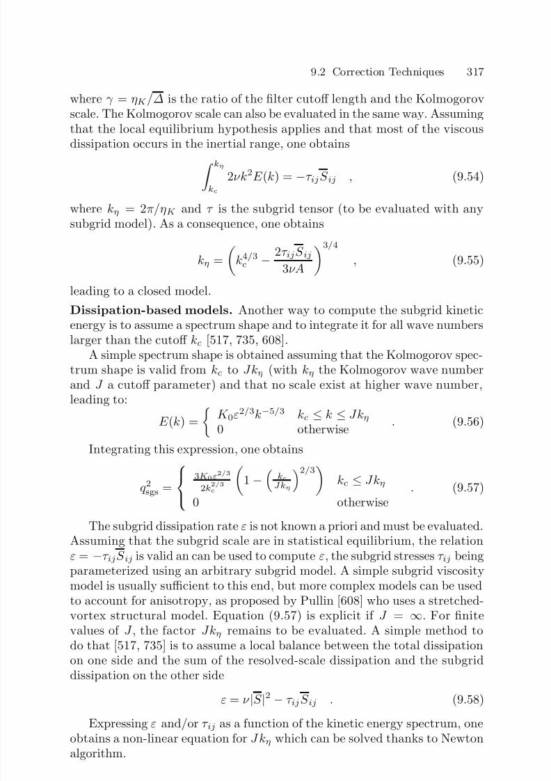
7/21/2019 Large Eddy Simulation for Incompressible Flows
http://slidepdf.com/reader/full/large-eddy-simulation-for-incompressible-flows 337/573
9.2 Correction Techniques 317
where γ = ηK /∆ is the ratio of the filter cutoff length and the Kolmogorovscale. The Kolmogorov scale can also be evaluated in the same way. Assumingthat the local equilibrium hypothesis applies and that most of the viscousdissipation occurs in the inertial range, one obtains kη
kc
2νk2E (k) = −τ ijS ij , (9.54)
where kη = 2π/ηK and τ is the subgrid tensor (to be evaluated with anysubgrid model). As a consequence, one obtains
kη = k4/3c
−
2τ ijS ij
3νA 3/4
, (9.55)
leading to a closed model.
Dissipation-based models. Another way to compute the subgrid kineticenergy is to assume a spectrum shape and to integrate it for all wave numberslarger than the cutoff kc [517, 735, 608].
A simple spectrum shape is obtained assuming that the Kolmogorov spec-trum shape is valid from kc to Jkη (with kη the Kolmogorov wave numberand J a cutoff parameter) and that no scale exist at higher wave number,leading to:
E (k) = K 0ε2/3k−5/3 kc ≤ k ≤ Jkη0 otherwise
. (9.56)
Integrating this expression, one obtains
q 2sgs =
3K 0ε2/3
2k2/3c
1 −
kcJkη
2/3
kc ≤ Jkη
0 otherwise. (9.57)
The subgrid dissipation rate ε is not known a priori and must be evaluated.Assuming that the subgrid scale are in statistical equilibrium, the relationε = −τ ijS ij is valid an can be used to compute ε, the subgrid stresses τ ij beingparameterized using an arbitrary subgrid model. A simple subgrid viscositymodel is usually sufficient to this end, but more complex models can be usedto account for anisotropy, as proposed by Pullin [608] who uses a stretched-vortex structural model. Equation (9.57) is explicit if J = ∞. For finitevalues of J , the factor Jkη remains to be evaluated. A simple method todo that [517, 735] is to assume a local balance between the total dissipationon one side and the sum of the resolved-scale dissipation and the subgriddissipation on the other side
ε = ν |S |2 − τ ijS ij . (9.58)
Expressing ε and/or τ ij as a function of the kinetic energy spectrum, oneobtains a non-linear equation for J kη which can be solved thanks to Newtonalgorithm.

7/21/2019 Large Eddy Simulation for Incompressible Flows
http://slidepdf.com/reader/full/large-eddy-simulation-for-incompressible-flows 338/573
318 9. Analysis and Validation
9.3 Practical Experience
Practice shows that nearly all authors make comparisons with reference dataor analyze large-eddy simulation data with no processing of the data. Theagreements observed with the reference data can then be explained by the factthat the quantities being compared are essentially related to scale ranges con-tained in the resolved field. This is generally true of the first-order moments(i.e. the mean velocity field) and, in certain cases, of the second-order mo-ments (the Reynolds stresses). This lack of processing prior to data analysisseems to be due mainly to the uncertainties in the techniques for evaluat-ing the contributions of the subgrid scales and to the difficulty of ad hocfiltering of the reference data. Large-eddy simulation also allows a satisfac-
tory prediction of the time frequency associated with large-scale periodic orquasi-periodic phenomena (such as vortex shedding) and the first harmonicsof this frequency for fine mesh.
One has to be careful when trying to recover high-order statistical datafrom large-eddy simulation. The two main reasons are:
– The properties of the exact filtered solution, i.e. the solution of an ideallarge-eddy simulation without numerical and modeling errors referred to asuΠ in Chap. 1, may be different from those of the exact unfiltered solution.
– Numerical and modeling errors can corrupt the field, yielding new errors.
Fig. 9.1. Comparison of time correlation versus a normalized time lag in isotropicturbulence. Upper curves are from Large-Eddy Simulation and lower curves fromDirect Numerical Simulation. Courtesy of S. Rubinstein, NASA.
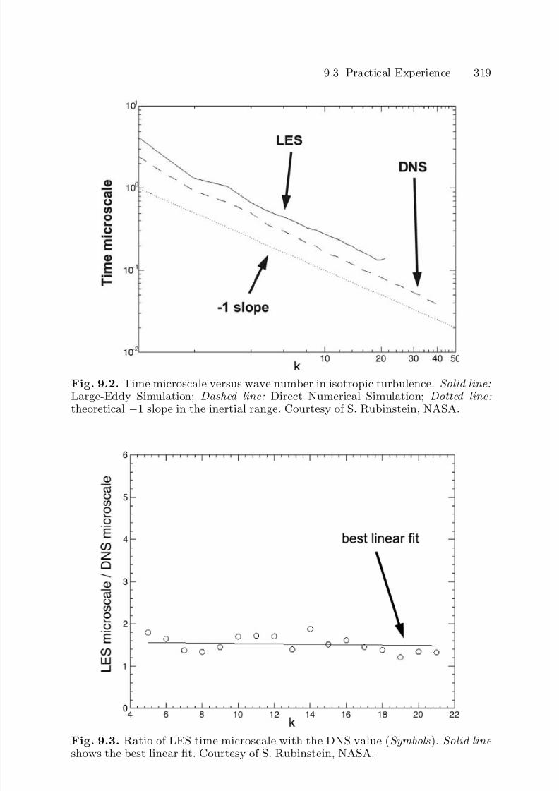
7/21/2019 Large Eddy Simulation for Incompressible Flows
http://slidepdf.com/reader/full/large-eddy-simulation-for-incompressible-flows 339/573
9.3 Practical Experience 319
Fig. 9.2. Time microscale versus wave number in isotropic turbulence. Solid line:Large-Eddy Simulation; Dashed line: Direct Numerical Simulation; Dotted line:theoretical
−1 slope in the inertial range. Courtesy of S. Rubinstein, NASA.
Fig. 9.3. Ratio of LES time microscale with the DNS value (Symbols ). Solid line shows the best linear fit. Courtesy of S. Rubinstein, NASA.
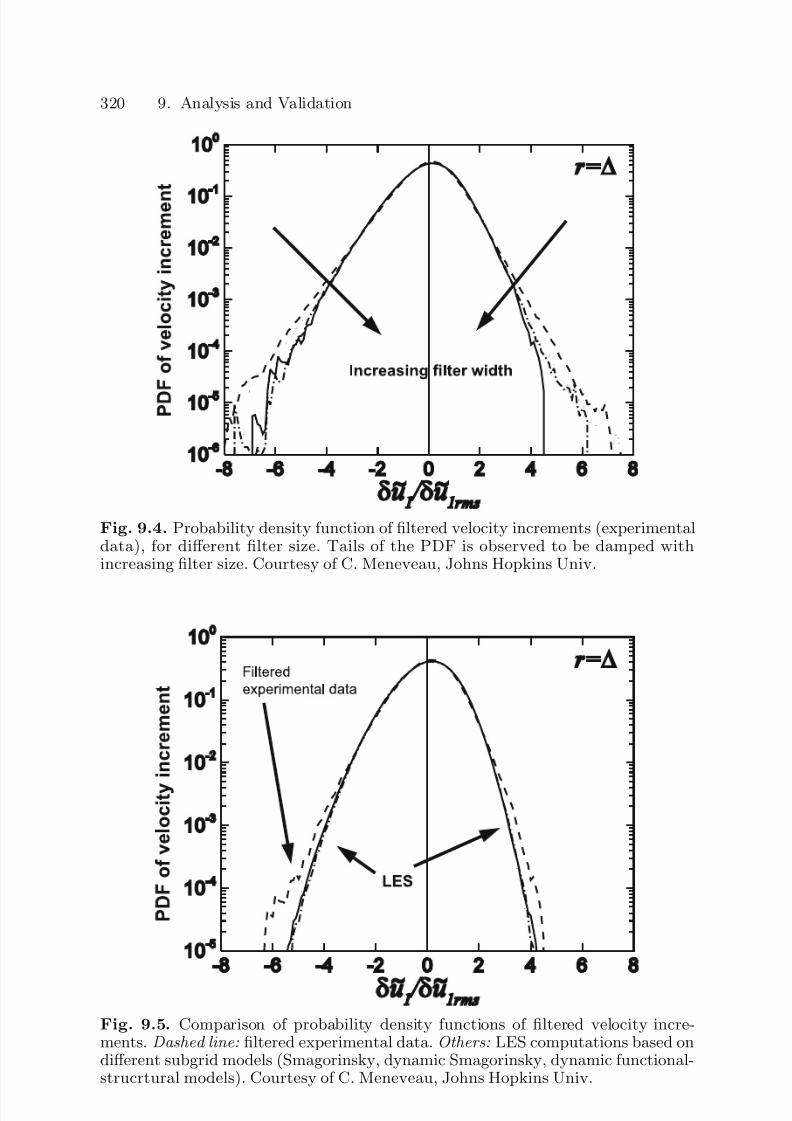
7/21/2019 Large Eddy Simulation for Incompressible Flows
http://slidepdf.com/reader/full/large-eddy-simulation-for-incompressible-flows 340/573
320 9. Analysis and Validation
Fig. 9.4. Probability density function of filtered velocity increments (experimentaldata), for different filter size. Tails of the PDF is observed to be damped withincreasing filter size. Courtesy of C. Meneveau, Johns Hopkins Univ.
Fig. 9.5. Comparison of probability density functions of filtered velocity incre-ments. Dashed line: filtered experimental data. Others: LES computations based ondifferent subgrid models (Smagorinsky, dynamic Smagorinsky, dynamic functional-strucrtural models). Courtesy of C. Meneveau, Johns Hopkins Univ.

7/21/2019 Large Eddy Simulation for Incompressible Flows
http://slidepdf.com/reader/full/large-eddy-simulation-for-incompressible-flows 341/573
9.3 Practical Experience 321
Fig. 9.6. Longitudinal velocity structure of order 6 and 10 plotted versus displace-ment. Squares: unfiltered data; Circles: filtered data. From [116].
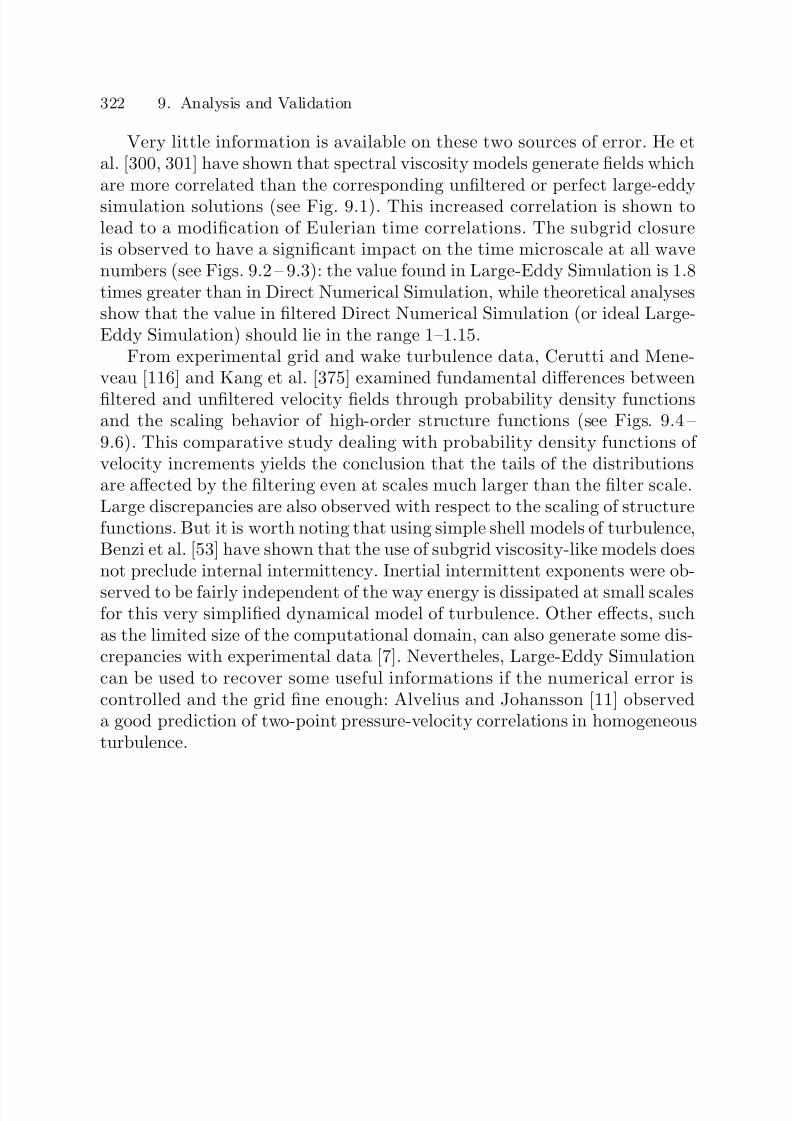
7/21/2019 Large Eddy Simulation for Incompressible Flows
http://slidepdf.com/reader/full/large-eddy-simulation-for-incompressible-flows 342/573
322 9. Analysis and Validation
Very little information is available on these two sources of error. He etal. [300, 301] have shown that spectral viscosity models generate fields whichare more correlated than the corresponding unfiltered or perfect large-eddysimulation solutions (see Fig. 9.1). This increased correlation is shown tolead to a modification of Eulerian time correlations. The subgrid closureis observed to have a significant impact on the time microscale at all wavenumbers (see Figs. 9.2 – 9.3): the value found in Large-Eddy Simulation is 1.8times greater than in Direct Numerical Simulation, while theoretical analysesshow that the value in filtered Direct Numerical Simulation (or ideal Large-Eddy Simulation) should lie in the range 1–1.15.
From experimental grid and wake turbulence data, Cerutti and Mene-veau [116] and Kang et al. [375] examined fundamental differences between
filtered and unfiltered velocity fields through probability density functionsand the scaling behavior of high-order structure functions (see Figs. 9.4 –9.6). This comparative study dealing with probability density functions of velocity increments yields the conclusion that the tails of the distributionsare affected by the filtering even at scales much larger than the filter scale.Large discrepancies are also observed with respect to the scaling of structurefunctions. But it is worth noting that using simple shell models of turbulence,Benzi et al. [53] have shown that the use of subgrid viscosity-like models doesnot preclude internal intermittency. Inertial intermittent exponents were ob-
served to be fairly independent of the way energy is dissipated at small scalesfor this very simplified dynamical model of turbulence. Other effects, suchas the limited size of the computational domain, can also generate some dis-crepancies with experimental data [7]. Nevertheles, Large-Eddy Simulationcan be used to recover some useful informations if the numerical error iscontrolled and the grid fine enough: Alvelius and Johansson [11] observeda good prediction of two-point pressure-velocity correlations in homogeneousturbulence.
7/21/2019 Large Eddy Simulation for Incompressible Flows
http://slidepdf.com/reader/full/large-eddy-simulation-for-incompressible-flows 343/573
10. Boundary Conditions
Like all the other approaches mentioned in the introduction, large-eddy simu-lation requires the setting of boundary conditions in order to fully determine
the system and obtain a mathematically well-posed problem. This chapter isdevoted to questions of determining suitable boundary conditions for large-eddy simulation computations. The first section is a discussion of generalorder, the second is devoted to the representation of solid walls, and thethird discusses methods used for representing an unsteady upstream flow.
10.1 General Problem
10.1.1 Mathematical Aspects
Many theoretical problems dealing with boundary conditions for large-eddysimulation can be identified. Two of the most important ones are the possibleinteraction between the filter and the exact boundary conditions, and thespecification of boundary conditions leading to the definition of a well-posedproblem.
From the results of Sects. 2.2 and 3.4, we deduce that the general form of the filtered Navier–Stokes equations on a bounded domain Ω is
∂ui∂t
+ ∂
∂xj(uiuj) +
∂p
∂xi− ν
∂
∂xj
∂ui∂xj
+ ∂uj∂xi
=
− ∂Ω
G(x−ξ)
ui(ξ)uj(ξ)+ p(ξ)−ν
∂ui(ξ)
∂xj+
∂uj(ξ)
∂xi
nj(ξ)dξ , (10.1)
∂ui∂xi
= − ∂Ω
G(x − ξ)ui(ξ)ni(ξ)dξ , (10.2)
where n is the outward unit normal vector to the boundary of Ω , ∂Ω . It
must be noted that only terms induced by the interaction of the filter and theboundaries have been retained, i.e. other commutation errors are neglected.Right-hand side terms in (10.1) and (10.2) are additional source terms, thatmust be modeled because they involve the non-filtered velocity and pressurefields.
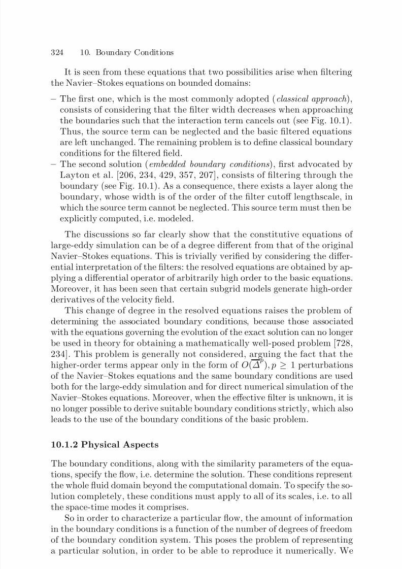
7/21/2019 Large Eddy Simulation for Incompressible Flows
http://slidepdf.com/reader/full/large-eddy-simulation-for-incompressible-flows 344/573
324 10. Boundary Conditions
It is seen from these equations that two possibilities arise when filteringthe Navier–Stokes equations on bounded domains:
– The first one, which is the most commonly adopted (classical approach ),consists of considering that the filter width decreases when approachingthe boundaries such that the interaction term cancels out (see Fig. 10.1).Thus, the source term can be neglected and the basic filtered equationsare left unchanged. The remaining problem is to define classical boundaryconditions for the filtered field.
– The second solution (embedded boundary conditions ), first advocated byLayton et al. [206, 234, 429, 357, 207], consists of filtering through theboundary (see Fig. 10.1). As a consequence, there exists a layer along the
boundary, whose width is of the order of the filter cutoff lengthscale, inwhich the source term cannot be neglected. This source term must then beexplicitly computed, i.e. modeled.
The discussions so far clearly show that the constitutive equations of large-eddy simulation can be of a degree different from that of the originalNavier–Stokes equations. This is trivially verified by considering the differ-ential interpretation of the filters: the resolved equations are obtained by ap-plying a differential operator of arbitrarily high order to the basic equations.Moreover, it has been seen that certain subgrid models generate high-order
derivatives of the velocity field.This change of degree in the resolved equations raises the problem of
determining the associated boundary conditions, because those associatedwith the equations governing the evolution of the exact solution can no longerbe used in theory for obtaining a mathematically well-posed problem [728,234]. This problem is generally not considered, arguing the fact that thehigher-order terms appear only in the form of O(∆
p), p ≥ 1 perturbations
of the Navier–Stokes equations and the same boundary conditions are usedboth for the large-eddy simulation and for direct numerical simulation of the
Navier–Stokes equations. Moreover, when the effective filter is unknown, it isno longer possible to derive suitable boundary conditions strictly, which alsoleads to the use of the boundary conditions of the basic problem.
10.1.2 Physical Aspects
The boundary conditions, along with the similarity parameters of the equa-tions, specify the flow, i.e. determine the solution. These conditions representthe whole fluid domain beyond the computational domain. To specify the so-
lution completely, these conditions must apply to all of its scales, i.e. to allthe space-time modes it comprises.So in order to characterize a particular flow, the amount of information
in the boundary conditions is a function of the number of degrees of freedomof the boundary condition system. This poses the problem of representinga particular solution, in order to be able to reproduce it numerically. We

7/21/2019 Large Eddy Simulation for Incompressible Flows
http://slidepdf.com/reader/full/large-eddy-simulation-for-incompressible-flows 345/573
10.1 General Problem 325
Fig. 10.1. Schematic of the classical approach (Top) and the embedded boundarycondition approach (Bottom ), in a solid wall configuration. In the classical approach
the cutoff length ∆ is reduced in the vicinity of the wall so that the interactionterm cancels out. In the second approach, the cutoff length is constant. Courtesyof E. Garnier, ONERA.

7/21/2019 Large Eddy Simulation for Incompressible Flows
http://slidepdf.com/reader/full/large-eddy-simulation-for-incompressible-flows 346/573
326 10. Boundary Conditions
have a new modeling problem here, which is that of modeling the physicaltest configuration.
This difficulty is increased for the large-eddy simulation and direct numer-ical simulation, because these simulations contain a large number of degreesof freedom and require a precise space-time deterministic representation of the solution at the computational domain boundaries.
Two special cases will be discussed in the following sections: that of rep-resenting solid walls and that of representing a turbulent inflow. The problemof the outflow conditions, which is not specific to the large-eddy simulationtechnique, will not be addressed1.
10.2 Solid Walls
10.2.1 Statement of the Problem
Specific Features of the Near-Wall Region. The structure of the bound-ary layer flow has certain characteristics that call for special treatment in theframework of large-eddy simulation. In this section, we describe the elementscharacteristic of the boundary layer dynamics and kinematics, which showsup the difference with an isotropic homogeneous turbulence. For a detailed
description, the reader may refer to [648, 150].Definitions. Here we adopt the ideal framework of a flat-plate, turbulentboundary layer, without pressure gradient. The external flow is in the (Ox)direction and the (Oz) direction is normal to the wall. The external velocity isdenoted U e. In the following, the Cartesian coordinate system will be denotedeither (x,y,z) or (x1, x2, x3), for convenience. Similarly, the velocity vectoris denoted (u,v,w) or (u1, u2, u3).
We first recall a few definitions. The boundary layer thickness δ is definedas the distance from the plate beyond which the fluid becomes irrotational,
and thus where the fluid velocity is equal to the external velocity.The wall shear stress τ p is defined as:
τ p =
τ 2p,13 + τ 2p,23 , (10.3)
in which τ p,ij = νS ij(x,y, 0). The friction velocity uτ is defined as:
uτ =√
τ p . (10.4)
In the case of the canonical boundary layer, we get:
uτ =
ν
∂u1
∂z (x,y, 0) . (10.5)
1 See [156] for a specific study of exit boundary conditions for the plane channelflow case.
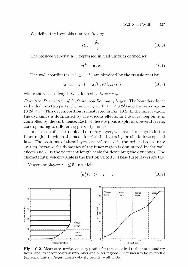
7/21/2019 Large Eddy Simulation for Incompressible Flows
http://slidepdf.com/reader/full/large-eddy-simulation-for-incompressible-flows 347/573
10.2 Solid Walls 327
We define the Reynolds number Reτ by:
Reτ =
δuτ
ν . (10.6)
The reduced velocity u+, expressed in wall units, is defined as:
u+ = u/uτ . (10.7)
The wall coordinates (x+, y+, z+) are obtained by the transformation:
(x+, y+, z+) = (x/lτ ,y/lτ ,z/lτ ) , (10.8)
where the viscous length lτ is defined as lτ = ν/uτ .
Statistical Description of the Canonical Boundary Layer. The boundary layeris divided into two parts: the inner region (0 ≤ z < 0.2δ ) and the outer region(0.2δ ≤ z). This decomposition is illustrated in Fig. 10.2. In the inner region,the dynamics is dominated by the viscous effects. In the outer region, it iscontrolled by the turbulence. Each of these regions is split into several layers,corresponding to different types of dynamics.
In the case of the canonical boundary layer, we have three layers in theinner region in which the mean longitudinal velocity profile follows special
laws. The positions of these layers are referenced in the reduced coordinatesystem, because the dynamics of the inner region is dominated by the walleffects and lτ is the pertinent length scale for describing the dynamics. Thecharacteristic velocity scale is the friction velocity. These three layers are the:
– Viscous sublayer: z+ ≤ 5, in which
u+1 (z+) = z + . (10.9)
Fig. 10.2. Mean streamwise velocity profile for the canonical turbulent boundarylayer, and its decomposition into inner and outer regions. Left : mean velocity profile(external units). Right : mean velocity profile (wall units).

7/21/2019 Large Eddy Simulation for Incompressible Flows
http://slidepdf.com/reader/full/large-eddy-simulation-for-incompressible-flows 348/573
328 10. Boundary Conditions
– Buffer layer: 5 < z+ ≤ 30, where
u+
1 (z+)
5 ln z+
−3.05 . (10.10)
– Prandtl or logarithmic inertial layer: 30 < z+; z/δ 1, for which
u+1 (z+) 1
κ ln z+ + 5, 5 ± 0, 1, κ = 0, 4 . (10.11)
The outer region includes the end of the logarithmic inertial region andthe wake region. In this zone, the characteristic length is no longer lτ butrather the thickness δ . The characteristic velocity scale remains unchanged,though. The average velocity profiles are described by:
– For the logarithmic inertial region:
u1(z)uτ
= A ln zuτ
ν + B , (10.12)
where A and B are constants;– For the wake region:
u1(z)uτ
= A ln zuτ
ν
+ B + Π
κ
W z
δ , (10.13)
where A, B and Π are constants and W the wake function defined byClauser as:
W (x) = 2 sin2(πx/2) . (10.14)
Concerning the Dynamics of the Canonical Boundary Layer. Experimentaland numerical studies have identified dynamic processes within the bound-ary layer. We will summarize here the main elements of the boundary layerdynamics that originate the turbulence in the near-wall region.
Observations show that the flow is highly agitated very close to the wall,consisting of pockets of fast and slow fluid that organize in ribbons parallelto the outer velocity (streaks, see Fig. 10.3). The low-velocity pockets mi-grate slowly outward in the boundary layer (ejection) and are subject to aninstability that makes them explode near the outer edge of the inner region.This burst is followed by an arrival of fast fluid toward the wall, sweepingthe near-wall region almost parallel to it. These highly intermittent eventsin time and space induce strong variation in the unsteady Reynolds stressesand originate a very large part of the production and dissipation of the tur-
bulent kinetic energy. These variations produce fluctuations in the subgriddissipation that can reach 300% of the average value and can make it changesign. Analyses of direct numerical simulations [291, 598, 449, 363] indicatethat a very intense small scale dissipation in the buffer region is correlatedwith the presence of sheared layers that form the interfaces between the fluidpockets of different velocities. These mechanisms are highly anisotropic. Their
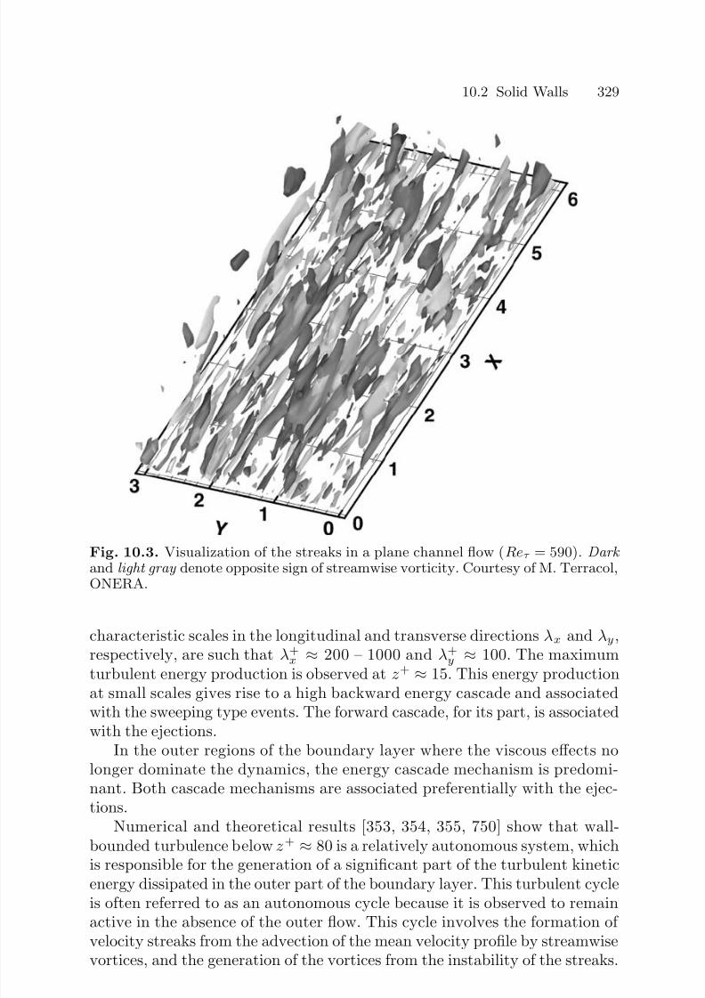
7/21/2019 Large Eddy Simulation for Incompressible Flows
http://slidepdf.com/reader/full/large-eddy-simulation-for-incompressible-flows 349/573
10.2 Solid Walls 329
Fig. 10.3. Visualization of the streaks in a plane channel flow (Reτ = 590). Dark and light gray denote opposite sign of streamwise vorticity. Courtesy of M. Terracol,ONERA.
characteristic scales in the longitudinal and transverse directions λx and λy,respectively, are such that λ+
x ≈ 200 – 1000 and λ+y ≈ 100. The maximum
turbulent energy production is observed at z+ ≈ 15. This energy production
at small scales gives rise to a high backward energy cascade and associatedwith the sweeping type events. The forward cascade, for its part, is associatedwith the ejections.
In the outer regions of the boundary layer where the viscous effects nolonger dominate the dynamics, the energy cascade mechanism is predomi-nant. Both cascade mechanisms are associated preferentially with the ejec-tions.
Numerical and theoretical results [353, 354, 355, 750] show that wall-bounded turbulence below z+ ≈ 80 is a relatively autonomous system, whichis responsible for the generation of a significant part of the turbulent kineticenergy dissipated in the outer part of the boundary layer. This turbulent cycleis often referred to as an autonomous cycle because it is observed to remainactive in the absence of the outer flow. This cycle involves the formation of velocity streaks from the advection of the mean velocity profile by streamwisevortices, and the generation of the vortices from the instability of the streaks.
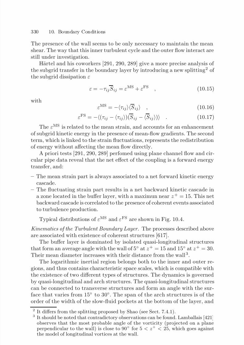
7/21/2019 Large Eddy Simulation for Incompressible Flows
http://slidepdf.com/reader/full/large-eddy-simulation-for-incompressible-flows 350/573
330 10. Boundary Conditions
The presence of the wall seems to be only necessary to maintain the meanshear. The way that this inner turbulent cycle and the outer flow interact arestill under investigation.
Hartel and his coworkers [291, 290, 289] give a more precise analysis of the subgrid transfer in the boundary layer by introducing a new splitting2 of the subgrid dissipation ε
ε = −τ ijS ij = εMS + εFS , (10.15)
withεMS = −τ ijS ij , (10.16)
εFS =−
(τ ij −
τ ij)(S ij
− S ij
)
. (10.17)
The εMS is related to the mean strain, and accounts for an enhancementof subgrid kinetic energy in the presence of mean-flow gradients. The secondterm, which is linked to the strain fluctuations, represents the redistributionof energy without affecting the mean flow directly.
A priori tests [291, 290, 289] perfomed using plane channel flow and cir-cular pipe data reveal that the net effect of the coupling is a forward energytransfer, and:
– The mean strain part is always associated to a net forward kinetic energy
cascade.– The fluctuating strain part results in a net backward kinetic cascade in
a zone located in the buffer layer, with a maximun near z + = 15. This netbackward cascade is correlated to the presence of coherent events associatedto turbulence production.
Typical distributions of εMS and εFS are shown in Fig. 10.4.
Kinematics of the Turbulent Boundary Layer. The processes described aboveare associated with existence of coherent structures [617].
The buffer layer is dominated by isolated quasi-longitudinal structuresthat form an average angle with the wall of 5 at z+ = 15 and 15 at z+ = 30.Their mean diameter increases with their distance from the wall3.
The logarithmic inertial region belongs both to the inner and outer re-gions, and thus contains characteristic space scales, which is compatible withthe existence of two different types of structures. The dynamics is governedby quasi-longitudinal and arch structures. The quasi-longitudinal structurescan be connected to transverse structures and form an angle with the sur-face that varies from 15 to 30. The span of the arch structures is of the
order of the width of the slow-fluid pockets at the bottom of the layer, and2 It differs from the splitting proposed by Shao (see Sect. 7.4.1).3 It should be noted that contradictory observations can be found. Lamballais [421]
observes that the most probable angle of the vorticity (projected on a planeperpendicular to the wall) is close to 90 for 5 < z + < 25, which goes againstthe model of longitudinal vortices at the wall.

7/21/2019 Large Eddy Simulation for Incompressible Flows
http://slidepdf.com/reader/full/large-eddy-simulation-for-incompressible-flows 351/573
10.2 Solid Walls 331
Fig. 10.4. Distribution of mean strain (εMS) and fluctuating strain (εFS) dissi-pations in a plane channel flow. Fluctuating strain is observed to yield dominantbackscatter near z + ∼ 15, but the total dissipation remains positive.
increases linearly with the distance from the wall. The relative number of quasi-longitudinal structures decreases with the distance from the wall, untilit cancels out at the beginning of the wake region.
The wake region is populated with arch structures forming an angle of 45 with the wall. Their x and y spacing is of the order of δ .
Resolving or Modeling. The description we have just made of the bound-ary layer flow structure clearly shows the problem of applying the large-eddysimulation technique in this case. Firstly, the mechanisms originating theturbulence, i.e. the flow driving mechanisms, are associated with fixed char-acteristic length scales on the average. Also, this turbulence production isassociated with a backward energy cascade, which is largely dominant overthe cascade mechanism in certain regions of the boundary layer. These twofactors make it so that the subgrid models presented in the previous chap-ters become inoperative because they no longer permit a reduction of thenumber of degrees of freedom while ensuring at the same time a fine repre-sentation of the flow driving mechanisms. There are then two possible ap-
proaches [536]:
– Resolving the near-wall dynamics directly. Since the production mecha-nisms escape the usual subgrid modeling, if we want to take them intoaccount, we have to use a sufficiently fine resolution to capture them. Thesolid wall is then represented by a no-slip condition: the fluid velocity is

7/21/2019 Large Eddy Simulation for Incompressible Flows
http://slidepdf.com/reader/full/large-eddy-simulation-for-incompressible-flows 352/573
332 10. Boundary Conditions
set equal to that of the solid wall. This equality implicitly relies on the hy-pothesis that the mean free path of the molecules is small compared withthe characteristic scales of the motion, and that these scales are large com-pared with the distance of the first grid point from the wall. In practice,this is done by placing the first point in the zone (0 ≤ z+ ≤ 1). To rep-resent the turbulence production mechanisms completely, Schumann [655]
recommends a spatial resolution such that ∆+1 < 10, ∆
+2 < 5 and ∆
+3 < 2.
Also, Zang [798] indicates that the minimum resolution for capturing the
existence of these mechanisms is ∆+1 < 80, ∆
+2 < 30 and that three grid
points should be located in the z+ ≤ 10 zone. Zahrai et al. [795] indicate
that ∆+1 100, ∆
+2 = 12 should be used as an upper limit if a second-
order accurate numerical method is used. These values are given here onlyfor reference, since larger values can also be found in the literature. For
example, Piomelli [591] uses ∆+1 = 244 for a plane channel flow. Chap-
man [119] estimates that representing the dynamics of the inner region,which contributes about one percent to the thickness of the full boundarylayer, requires O(Re1.8) degrees of freedom, while only O(Re0.4) are needed
to represent the outer zone. This corresponds to ∆+1 100, ∆
+2 20 and
∆+
3 < 2. Considering that non-isotropic modes must be directly resolved,Bagget et al. [32] show that the number of degrees of freedom of the solu-
tion (in space) scales as Re2τ .– Modeling the near-wall dynamics. To reduce the number degrees of freedom
and especially avoid having to represent the inner region, we use a modelfor representing the dynamics of that zone. This is a special subgrid modelcalled the wall model. Since the distance from the first grid point to thewall is greater than the characteristic scales of the modes existing in themodeled region, the no-slip condition can no longer be used. The boundarycondition will apply to the values of the velocity components and/or theirgradients, which will be provided by the wall model. This approach makes
it possible to place the first point in the logarithmic layer (in practice,20 ≤ z+ ≤ 200). The main advantage of this approach is that the numberof degrees of freedom in the simulation can be reduced greatly; but sincea part of the dynamics is modeled, it constitutes an additional source of error.
10.2.2 A Few Wall Models
In the following, we present the most popular wall models for large-eddy
simulation. These models all represent an impermeable wall, and most of them have been implemented using a staggered grid (see Fig. 10.5). The dis-cussion will be restricted to wall models defined on Cartesian body-fittedcomputational grids. Details dealing with implementation on curvilinearbody-fitted grids or on Cartesian grids using the immersed boundary tech-nique [35, 713, 271, 270] will not be discussed, since they would require an

7/21/2019 Large Eddy Simulation for Incompressible Flows
http://slidepdf.com/reader/full/large-eddy-simulation-for-incompressible-flows 353/573
10.2 Solid Walls 333
Fig. 10.5. Illustration of a staggered grid system in the streamwise/wall-normalplane.
extensive discussion about numerical methods which is far beyond the scopeof this book.
Existing strategies for the definition of wall models for large-eddy simu-lation following the classical approach can be grouped in several classes:
– Higher-order boundary conditions : velocity gradients at the wall are con-trolled by enforcing boundary conditions on second-order derivatives. Thisclass is represented by Deardorff’s model (p. 337).
– Wall stress models : the first mesh at the wall is chosen to be very large, sothat it is not able to respresent correctly the dynamics of the inner layer.Typical dimensions are 100 wall units in the wall-normal and spanwisedirections and 500 wall units in the streamwise direction. This is illustratedin Fig. 10.7, where it is clearly observed that the near-wall events areaveraged over the first grid cell. The wall model should provide the value
of wall stresses, which cannot be accurately directly computed on the gridbecause of its coarseness (see Fig. 10.6), and the value of the wall-normalvelocity component.The basic form of these stress models is
τ i,3 = F (u1, z2) , i = 1, 2 , (10.18)
where z2 is the height of the first cell. If the flow is bidimensional andlaminar, a trivial relation is
τ 1,3 = −ν u1
z2/2 . (10.19)
A first group of wall-stress models is based on the extrapolation of thislinear, laminar law, the molecular viscosity being replaced by an effectiveturbulent viscosity, ν eff . Recalling that the total mean shear stress is almost

7/21/2019 Large Eddy Simulation for Incompressible Flows
http://slidepdf.com/reader/full/large-eddy-simulation-for-incompressible-flows 354/573
334 10. Boundary Conditions
Fig. 10.6. Computed value of the mean wall shear stress (with reference to itsexact value), expressed as a function of the distance of the first off-wall grid point.
constant across the inner part of the boundary layer, we have:
τ 13(z) = −ν tot(z)∂ u1(z)
∂z τ p,13 , (10.20)
where ν tot(z) is the sum of the molecular and the turbulent viscosity. Byintegrating (10.20) in the wall-normal direction, we obtain:
z
0
τ 13(z)ν tot(z)
dz = − z
0
∂ u1(z)∂z
dz , (10.21)
leading to
τ p,13 z
0
1
ν tot(z)dz = −u1(z) , (10.22)
and, finally,
τ p,13 = −
1
z
z0
1
ν tot(z)dz
−1
ν eff
u1(z)z
. (10.23)
The wall-stress models discussed below are:1. The Schumann model (p. 339), which relies on a linear relation between
the wall stress and the velocity component at the first off-wall grid point.The skin friction is an entry parameter for the model.
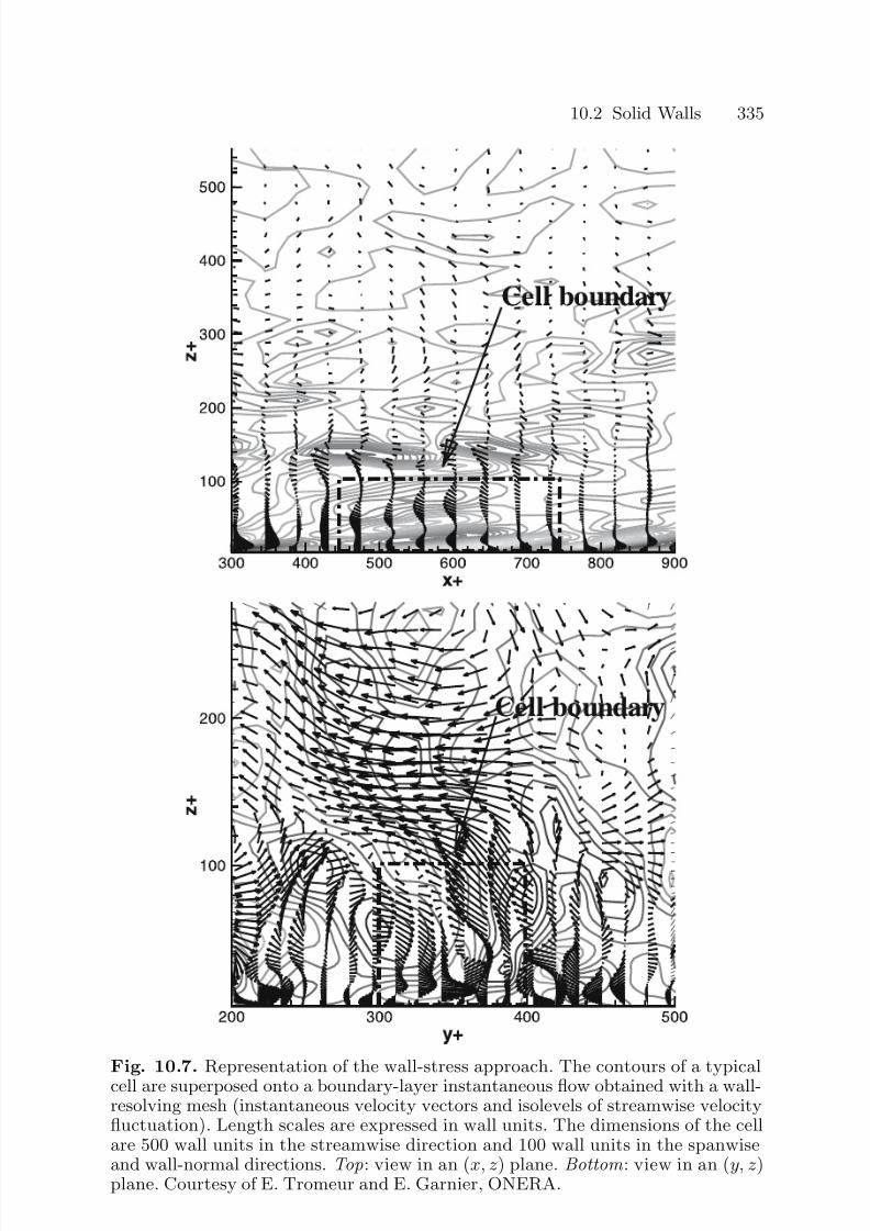
7/21/2019 Large Eddy Simulation for Incompressible Flows
http://slidepdf.com/reader/full/large-eddy-simulation-for-incompressible-flows 355/573
10.2 Solid Walls 335
Fig. 10.7. Representation of the wall-stress approach. The contours of a typicalcell are superposed onto a boundary-layer instantaneous flow obtained with a wall-resolving mesh (instantaneous velocity vectors and isolevels of streamwise velocityfluctuation). Length scales are expressed in wall units. The dimensions of the cellare 500 wall units in the streamwise direction and 100 wall units in the spanwiseand wall-normal directions. Top: view in an (x, z ) plane. Bottom : view in an (y, z )plane. Courtesy of E. Tromeur and E. Garnier, ONERA.

7/21/2019 Large Eddy Simulation for Incompressible Flows
http://slidepdf.com/reader/full/large-eddy-simulation-for-incompressible-flows 356/573
336 10. Boundary Conditions
2. The Grotzbach model (p. 339), which is an extension of the Schumannmodel. The skin friction is now computed assuming that the flow cor-responds to the canonical flat-plate boundary layer. The skin frictionis computed by inverting the logarithmic law profile for the streamwisevelocity.
3. The shifted correlations model (p. 340), which extends the Grotzbachmodel by taking into account explicitly the fact that fluctuations aregoverned by coherent structures with given time- and lengthscales.
4. The ejection model (p. 341), which is another extension of the model of Grotzbach. It takes into account the effects of sweep and ejection eventson the wall shear stress.
5. The optimized ejection model (p. 341), which is based on experimental
correlation data and yields better correlation coefficient in a priori tests.6. The model of Werner and Wengle (p. 344), which can be seen as a variant
of the Grotzbach model based on power-law profiles for the streamwisevelocity instead of the logarithmic law. The main advantage is that thepower law can be inverted explicitly.
7. The modified Werner–Wengle model (p. 345), which accounts for theexistence of ejection, as the model proposed by Piomelli.
8. The model of Murakami et al. (p. 343), which can be interpreted asa simplified version of the preceding model.
9. The model of Mason and Callen for rough walls (p. 340).10. The suboptimal-control-based wall models (p. 345). Numerical exper-
iments show that the previous wall stress models are not robust, i.e.they lead to disappointing results on very coarse mesh for high Reynoldsnumbers. This is mainly due to the fact that they can not account forlarge numerical and physical errors occuring on such coarse grids. Thesenew models, developed within the framework of suboptimal control, aimat producing the best possible results.
The second group of wall-stress models relies on the use of an internal layernear the wall, leading to the definition of two-layer simulations. Anotherset of governing equations is solved on an auxiliary grid located inside thefirst cell of the large-eddy simulation grid. An effective gain is obtainedif the auxiliary simulation can be run on a much coarser grid than large-eddy simulation while guaranteeing the accuracy of the results, or if theauxiliary equations are much simpler than the Navier–Stokes equations.Models belonging to this group are:
1. The thin-boundary-layer equation model developed by Balaras et al.(p. 342). The governing equations solved in the inner layer are the bound-
ary layer equations derived from the Navier–Stokes equations. The gaincomes from the fact that the pressure is assumed to be constant acrossthe boundary layer, and the pressure is not computed.
2. The wall model based on Kerstein’s ODT approach (p. 350). Thismodel relies on the reconstruction of the solution in the inner layer via
7/21/2019 Large Eddy Simulation for Incompressible Flows
http://slidepdf.com/reader/full/large-eddy-simulation-for-incompressible-flows 357/573
10.2 Solid Walls 337
a simplified one-dimensional stochastic system. It can be interpreted asa surrogate of the model based on the full boundary layer equations.
3. Hybrid RANS/LES approaches, in which a RANS-like simulation is per-formed in the near-wall region, while the core of the flow is treated bylarge-eddy simulation. All these models and techniques are discussed inChap. 12, with emphasis in Sect. 12.2.
– Off-wall boundary conditions : the mesh is built so that the first point islocated in the fluid region, and not on the wall. The first grid line parallelto the wall must be located in the inner region of the boundary layer. Thisapproach is illustrated in Fig. 10.8. An important point is that the gridmust still be able to represent details of the flow, and thus the mesh should
be the same as those used for wall-resolving simulation away from the wall.Several types of boundary conditions can be used following this approach,dealing either with the velocity components or their derivatives [30, 568,356]. Poor results have been obtained using that approach, which requiresvery accurate structural information on the fluctuations to yield accurateresults. Jimenez and Vasco [356] showed that the flow is very sensitiveto the prescribed wall-normal velocity component (transpiration velocity ),which must satisfy the continuity constraint.4 The need for an instanta-neous non-zero transpiration velocity can easily be understood by looking
at the velocity field displayed in Fig. 10.8.The usual failure of these models leads to the appearance of a strong,spurious boundary layer above the artificial boundary.
– Deterministic minimal boundary-layer unit simulation . Pascarelli et al.[580] proposed performing a wall-resolved temporal large-eddy simulationon the smallest domain allowing the existence of the near-wall autonomouscycle, and duplicating it. This approach leads to the definition of a crystalof elementary chaotic dynamical systems. The associated numerical tech-nique corresponds to a multiblock approach. Nonlinear interactions areexpected to scramble the data in the outer part of the boundary layer andto break possible periodicity.
The wall-model developed by Das and Moser within the framework of embedded boundary conditions is presented on p. 349.
Deardorff’s Model. In the framework of a plane channel simulation withinfinite Reynolds number, Deardorff [172] proposes using the following con-ditions for representing the solid walls:
∂ 2u1
∂z2
=
− 1
κ(z2/2)2
+ ∂ 2u1
∂y2
, (10.24)
4 This conclusion must be considered together with the fact that the best resultsobtained with wall-stress models are with non-zero transpiration velocity (seesuboptimal models, p. 345). A general conclusion is that even for impermeablewalls a non-zero wall-normal velocity must be prescribed to accurately describethe near-wall dynamics.

7/21/2019 Large Eddy Simulation for Incompressible Flows
http://slidepdf.com/reader/full/large-eddy-simulation-for-incompressible-flows 358/573
338 10. Boundary Conditions
Fig. 10.8. Representation of the off-wall approach. The grid lines are superposedto a boundary-layer instantaneous flow obtained with a wall-resolving mesh (instan-taneous velocity vectors and isolevels of streamwise velocity fluctuation). Lengthscales are expressed in wall units. The first grid point is located at 100 wall units.Top: view in an (x, z ) plane. Bottom : view in an (y, z ) plane.

7/21/2019 Large Eddy Simulation for Incompressible Flows
http://slidepdf.com/reader/full/large-eddy-simulation-for-incompressible-flows 359/573
10.2 Solid Walls 339
u3 = 0 , (10.25)
∂ 2u2
∂z 2
= ∂ 2u2
∂x2
, (10.26)
where z2 is the distance from the first point to the wall and κ = 0.4 theVon Karman constant. The first condition assumes that the average velocityprofile verifies the logarithmic law and that the second derivatives of the fluc-tuation u = u −u in the y and z directions are equal. The impermeabilitycondition (10.25) implies that the resolved stresses u1u3, u3u3 and u2u3 arezero at the wall. This model suffers from a number of defects. Namely, itshows no dependency as a function of the Reynolds number, and assumes
that the shear-stress near the wall is entirely due to the subgrid scales.Schumann Model. Schumann [653] has developed a wall model for per-forming a plane channel flow simulation at a finite Reynolds number. It isbased on the extended turbulent relation (10.23). Using dimensional analysis,the effective viscosity can be evaluated using
ν eff = z2
2
τ pu1(x,y,z2) . (10.27)
The resulting boundary conditions are:
τ p,13(x, y) =
u1(x,y,z2)
u1(x,y,z2)
τ p , (10.28)
u3 = 0 , (10.29)
τ p,23(x, y) = 2
Reτ
u3(x,y,z2)
z2
, (10.30)
where
designates a statistical average (associated here with a time aver-age), and z2 the distance of the first point to the wall. The condition (10.28)is equivalent to adopting the hypothesis that the longitudinal velocity com-ponent at position z2 is in phase with the instantaneous wall shear stress. Themean velocity profile can be obtained by the logarithmic law, and the meanwall shear stress τ p is, for a plane channel flow, equal to the driving pres-sure gradient. This wall model therefore implies that the mean velocity fieldverifies the logarithmic law and can be applied only to plane channel flowsfor which the value of the driving pressure gradient is known a priori. Thesecond condition is the impermeability condition, and the third correspondsto a no-slip condition for the transverse velocity component u2.
Grotzbach Model. Grotzbach [278] proposes extending the Schumannmodel to avoid having to know the mean wall shear stress a priori . To dothis, the statistical average is now associated with a mean on the planeparallel to the solid wall located at z = z2. Knowing u1(z2), the mean wall

7/21/2019 Large Eddy Simulation for Incompressible Flows
http://slidepdf.com/reader/full/large-eddy-simulation-for-incompressible-flows 360/573
340 10. Boundary Conditions
shear stress τ p is computed from the logarithmic law. The friction velocityis computed from (10.11), i.e.:
u+1 (z2) = u1(z2)/uτ = 1
κ log(z2uτ /ν ) + 5.5 ± 0.1 , (10.31)
then τ p, by relation (10.4). This model is more general than Schumann’s,but it still requires that the mean velocity profile verify the logarithmic law.Another advantage of Grotzbach’s modification is that it allows variations of the total mass flux through the channel.
Shifted correlations Model. Another modification of Schumann’s modelcan be made on the basis of the experimental works of Rajagopalan and
Antonia [614]. These two authors observed that the correlation between thewall shear stress and the velocity increases when we consider a relaxation timebetween these two evaluations. This phenomenon can be explained by theexistence of coherent inclined structures that are responsible for the velocityfluctuations and the wall shear stress. The modified model is expressed [595]:
τ p,13(x, y) =
u1(x + ∆s, y , z2)
u1(x,y,z2)
τ p , (10.32)
u3 = 0 , (10.33)
τ p,23(x, y) =
u2(x + ∆s, y , z2)
u1(x,y,z2)
τ p , (10.34)
where the value of the length ∆s is given by the approximate relation:
∆s =
(1 − z2) cot(8) for 30 ≤ z+2 ≤ 50–60
(1 − z2) cot(13) for z+2 ≥ 60
. (10.35)
Rough Wall Model. Mason and Callen [497] propose a wall model includ-ing the roughness effects. The three velocity components are specified at thefirst computation point by the relations:
u1(x,y,z2) = cos θ
uτ (x, y)
κ
ln(1 + z2/z0) , (10.36)
u2(x,y,z2) = sin θuτ (x, y)
κ ln(1 + z2/z0) , (10.37)
u3(x,y,z2) = 0 , (10.38)
where z0 is the roughness thickness of the wall and angle θ is given by therelation θ = arctan(u2(z2)/u1(z2)). These equations can be used to computethe friction velocity uτ as a function of the instantaneous velocity components
7/21/2019 Large Eddy Simulation for Incompressible Flows
http://slidepdf.com/reader/full/large-eddy-simulation-for-incompressible-flows 361/573
10.2 Solid Walls 341
u1 and u2. The instantaneous surface friction vector u2τ is then evaluated as:
u
2
τ =
1
M |u|u , (10.39)
where u is the vector (u1(x,y,z2), u2(x,y,z2), 0) and
1
M =
1
κ2 ln2(1 + z2/z0) .
The instantaneous wall shear stresses in the x and y directions are thenevaluated respectively as |u2
τ | cos θ and |u2τ | sin θ. This model is based on the
hypothesis that the logarithmic distribution is verified locally and instanta-
neously by the velocity field. This becomes even truer as the grid is coarsened,and the large scale velocity approaches the mean velocity.
Ejection Model. Another wall model is proposed by Piomelli, Ferziger,Moin, and Kim [595] in consideration of the fact that the fast fluid motionstoward or away from the wall greatly modify the wall shear stress. The impactof fast fluid pockets on the wall causes the longitudinal and lateral vortex linesto stretch out, increasing the velocity fluctuations near the wall. The ejectionof fast fluid masses induces the inverse effect, i.e. reduces the wall shear stress.To represent the correlation between the wall shear stress and the velocity
fluctuations, the authors propose the following conditions:
τ p,13(x, y) = τ p − Cuτ u3(x + ∆s, y , z2) , (10.40)
τ p,23(x, y) =
τ pu1(z2)
u2(x + ∆s, y , z2) , (10.41)
u3(x, y) = 0 , (10.42)
where C is a constant of the order of unity, τ p is computed from the log-
arithmic law as it is for the Grotzbach model, and ∆s is computed by therelation (10.35).
Marusic’s Optimized Ejection Model. Piomelli’s ejection wall modelwas futher improved by Marusic et al. [492] on the grounds of very accuratewind tunnel experiments. The proposed generalization for relation (10.40)based on the experimental correlations is
τ p,13(x, y) = τ p − αuτ (u1(x + ∆s, y , z2) − u1(x,y,z2)) , (10.43)
where α is a parameter taken equal to 0.1 for zero pressure gradient flows.This new ejection model, which is based on the streamwise velocity compo-nent instead of the wall-normal velocity in Piomelli’s original model, is foundto yield better results on priori tests carried out using experimental data: thecomputed peak correlation coefficient is in the range 0.34–0.53 for the newmodel while it is between 0.19 and 0.24 for the original model.
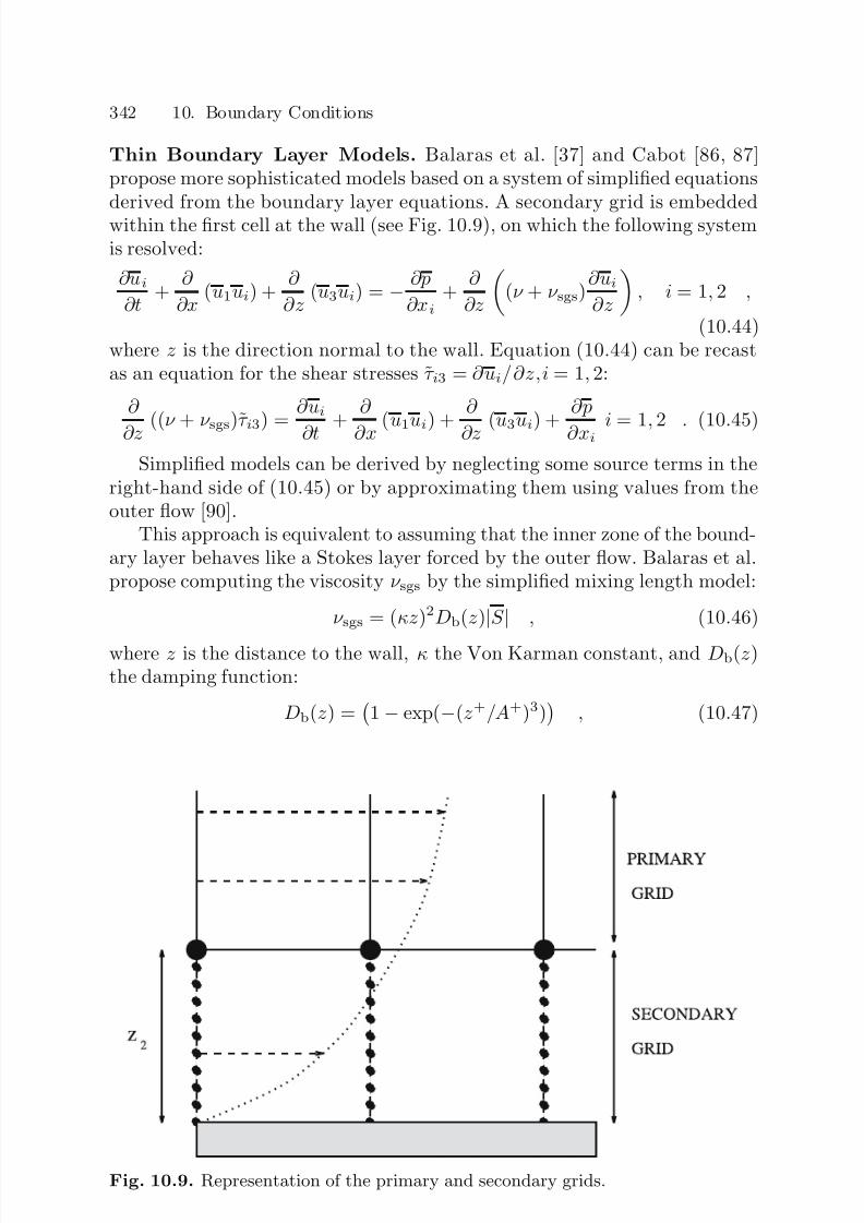
7/21/2019 Large Eddy Simulation for Incompressible Flows
http://slidepdf.com/reader/full/large-eddy-simulation-for-incompressible-flows 362/573
342 10. Boundary Conditions
Thin Boundary Layer Models. Balaras et al. [37] and Cabot [86, 87]propose more sophisticated models based on a system of simplified equationsderived from the boundary layer equations. A secondary grid is embeddedwithin the first cell at the wall (see Fig. 10.9), on which the following systemis resolved:
∂ui∂t
+ ∂
∂x (u1ui) +
∂
∂z (u3ui) = − ∂p
∂xi+
∂
∂z
(ν + ν sgs)
∂ui∂z
, i = 1, 2 ,
(10.44)where z is the direction normal to the wall. Equation (10.44) can be recastas an equation for the shear stresses τ i3 = ∂ui/∂z,i = 1, 2:
∂
∂z ((ν + ν sgs)τ i3) =
∂ui
∂t +
∂
∂x (u1ui) +
∂
∂z (u3ui) +
∂p
∂xi i = 1, 2 . (10.45)
Simplified models can be derived by neglecting some source terms in theright-hand side of (10.45) or by approximating them using values from theouter flow [90].
This approach is equivalent to assuming that the inner zone of the bound-ary layer behaves like a Stokes layer forced by the outer flow. Balaras et al.propose computing the viscosity ν sgs by the simplified mixing length model:
ν sgs = (κz)2Db(z)|S | , (10.46)
where z is the distance to the wall, κ the Von Karman constant, and Db(z)the damping function:
Db(z) =
1 − exp(−(z+/A+)3)
, (10.47)
Fig. 10.9. Representation of the primary and secondary grids.
7/21/2019 Large Eddy Simulation for Incompressible Flows
http://slidepdf.com/reader/full/large-eddy-simulation-for-incompressible-flows 363/573
10.2 Solid Walls 343
with A+ = 25. Cabot proposes the alternate definition:
ν sgs = κuszD2C (z) , (10.48)
in whichDC (z) = (1 − exp(−zud/Aν )) , (10.49)
where us and ud are velocity scales to be determined, and A = 19. Thesimplest choice is us = ud = uτ .
Cabot and Moin [90] observed that the constant of the mixing lengthmodel must be lowered in regard to its usual value in RANS computations inorder to account for resolved stresses. A dynamic evaluation of this constantwas achieved by Wang [751] to deal with flows with strong favorable/adverse
pressure gradient and incipient separation. The dynamic adjustment is per-formed by imposing that the mixing-length viscosity and the subgrid viscosityare equal at the interface of the two simulations.
When this system is solved, it generates longitudinal and transverse ve-locity component distributions at each time step, so that the value of the wallshear stress can be calculated for solving the filtered Navier–Stokes equationson the main grid. The pressure gradient appears as a source term, becausethis is obtained using the relation ∂p/∂xn = 0.
The vertical velocity component is obtained from the continuity equation:
u3(x,y,z2) = − z2
0
∂u1
∂x (x,y,ξ ) +
∂u2
∂y (x,y,ξ )
dξ . (10.50)
The boundary conditions applied to the secondary system are:
– On the solid wall: no-slip condition;– On the upper boundary: Dirichlet condition obtained from the value of the
velocity field computed on the first cell of the main grid.
Model of Murakami et al. Murakami, Mochida, and Hibi [556] developed
a wall model for dealing with the case of the separated flow around a cubemounted on a flat plate. This model is based on power-law solutions for themean longitudinal velocity profile of the form:
u1(z)U e
z
δ
n. (10.51)
The authors recommend using n = 1/4 on the flat plate and n = 1/2 onthe cube surface. When the first grid point is located close enough to thewall, the following boundary conditions are used:
ui(x, y) =
z2
z2 + ∆z
nui(x,y,z2 + ∆z), i = 1, 2 , (10.52)
u3(x, y) = 0 , (10.53)

7/21/2019 Large Eddy Simulation for Incompressible Flows
http://slidepdf.com/reader/full/large-eddy-simulation-for-incompressible-flows 364/573
344 10. Boundary Conditions
where ∆z is the size of the first cell. The first equation is obtained by assumingthat the instantaneous profile also verifies the law (10.51). When the distanceof the first point from the wall is too large for the convection effects to beneglected, the relation (10.53) is replaced by:
∂u3
∂z = 0 . (10.54)
Werner–Wengle Model. In order to be able to compute the same flow asMurakami et al., Werner and Wengle [757] propose a wall model based onthe following hypotheses:
– The instantaneous tangential velocity components at the wall u2(x,y,z2)
and u3(x,y,z2) are in phase with the associated instantaneous wall shearstresses.
– The instantaneous velocity profile follows the law:
u+(z) =
z+ if z+ ≤ 11.81
A(z+)B otherwise , (10.55)
in which A = 8.3 and B = 1/7.The values of the tangential velocity components can be related to the
corresponding values of the wall shear stress components by integrating thevelocity profile (10.55) over the distance separating the first cell from the wall.This allows a direct analytical evaluation of the wall shear stress componentsfrom the velocity field:
– If |ui(x,y,z2)| ≤ ν 2zm
A2/(1−B), then:
τ p,i3(x, y) = 2νui(x,y,z2)
z2, (10.56)
– and otherwise:
τ p,i3(x, y) = ui(x,y,z2)
|ui(x,y,z2)|
1 − B
2 A
1+B1−B
ν
z2
1+B
+1 + B
A
ν
z2
B|ui(x,y,z2)|
21+B
, (10.57)
where zm is the distance to the wall that corresponds to z+ = 11.81. Thismodel has the advantage of not using average statistical values of the velocityand/or wall shear stresses, which makes it easier to use for inhomogeneousconfigurations. An impermeability condition is used to specify the value of the velocity component normal to the wall:
u3 = 0 . (10.58)
7/21/2019 Large Eddy Simulation for Incompressible Flows
http://slidepdf.com/reader/full/large-eddy-simulation-for-incompressible-flows 365/573
10.2 Solid Walls 345
Werner–Wengle-Type Ejection Model. A version of the Werner–Wenglemodel which accounts for the shift that exists in the correlation betweenthe wall friction and the instantaneous velocity is proposed by Hassan andBarsamian [298]. The authors recommend to account for this shift as inPiomelli’s shifted model, leading to the following modifications for rela-tion (10.57)
τ p,i3(x, y) = ui(x + ∆s, y , z2)
|ui(x + ∆s, y , z2)|
1 − B
2 A
1+B1−B
ν
z2
1+B
+1 + B
A ν
z2B
|ui(x + ∆s, y , z2)| 2
1+B
−Cuτ u3(x + ∆s, y , z2) , (10.59)
where C is a constant of the order of the unity and ∆s is computed usingthe relation (10.35). Equation (10.56) is kept unchanged, since the shift isassumed to be negligible in the viscous sublayer.
Suboptimal-Control-Based Wall Models. The goal of this approachis to provide numerical boundary conditions so that the overall error (tobe defined) is minimum in a given norm. The boundary conditions (wallstresses and wall-normal velocity component) are used as a control to mini-
mize a cost function at each time step. Many variants of this approach canbe defined [566, 33], considering different degrees of freedom at the bound-ary (i.e. different controllers), different cost functions and different ways toevaluate the gradient of the cost function with respect to the controller.
Nicoud et al. [566] and Bagget et al. [33] considered a control vector φ onthe boundary whose components are the usual output of a wall-stress model:
φ = (τ p,13, u3, τ p,23) . (10.60)
The control can then be exerted by modifying both the stress at the wall
and the wall-normal transpiration velocity.The general form of the cost function J (u; φ) is defined as
J (u; φ) =3i=1
J mean,i(u; φ) +3i=1
J rms,i(u; φ) +3i=1
J penalty(φ) , (10.61)
where the terms appearing on the right-hand side are, from left to right: thepart of the cost based on the mean flow, the part of the cost based on the rmsvelocity fluctuations, and a penalty term representing the cost of the control.
The mean-flow part of the cost function is typically a measure of thedifference between the computed mean flow and a target mean flow uref . Forthe plane channel flow, it can be expressed as
J mean,i(u; φ) = αi1
2h
h−h
eui(z)2dz , (10.62)
7/21/2019 Large Eddy Simulation for Incompressible Flows
http://slidepdf.com/reader/full/large-eddy-simulation-for-incompressible-flows 366/573
346 10. Boundary Conditions
with
eui(z) = 1
A (ui(x,y,z) − U ref ,i(z))dxdy , (10.63)
where A is the surface of computational planes parallel to the walls and αiis an arbitrary weighting factor. The target mean flow can be prescribedusing experimental data, RANS simulations or theory. In a similar way, therms-based cost function is defined as
J rms,i(u; φ) = β i1
2h
h−h
eui(z)2dz , (10.64)
with
eui(z) = 1
A
(ui(x,y,z) − ui(z))2 − u2ref ,i(z)
dxdy , (10.65)
where ui is the average of the computed flow over homogeneous directions,β i is an arbitrary parameter, and u2ref ,i(z) are prescribed rms velocity profiles.
Bagget et al. proposed the following form of the penalty term:
J penalty(φ) = γ iA
z=±h
φ2uidxdy +
λ
A
z=±h
δ i3φ4u3dxdy , (10.66)
where γ i and λ are arbitrary constants. The last term of the penalty termprevents the transpiration velocity from becoming too high.
Several tests have been carried out, dealing with different weights of thethree parts of the cost function and the possibility of having a non-zerotranspiration velocity. The main results are:
– Suboptimal-control-based models lead to better results than usual wall-stress models (see Fig. 10.10). An interesting feature of these models isthat they are able to break the spurious linear dependence of the predictedwall stresses with respect to the instantaneous velocity at the first off-wallgrid point. This is observed by looking at Figs. 10.11 and 10.12.
– The use of a non-zero transpiration velocity makes it possible to improvesignificantly the mean flow profile compared to usual wall-stress models, if the rms part of the cost function is not considered (β i = 0). But, in thatcase, rms velocity profiles are not improved and prediction can even beworse.
– Rms velocity profiles can be improved if both J mean,i and J rms,i are takeninto account, but the improvement of the prediction of the mean velocityprofile is less important than in the previous case. The use of the non-zero
transpiration velocity is also observed to be beneficial.
This class of wall model based on the suboptimal control theory can beconsidered as the best achievable wall-stress model, and it seems difficultto get much better results controlling the same parameters (wall stresses andtranspiration velocity). Then, an interesting conclusion is that getting the
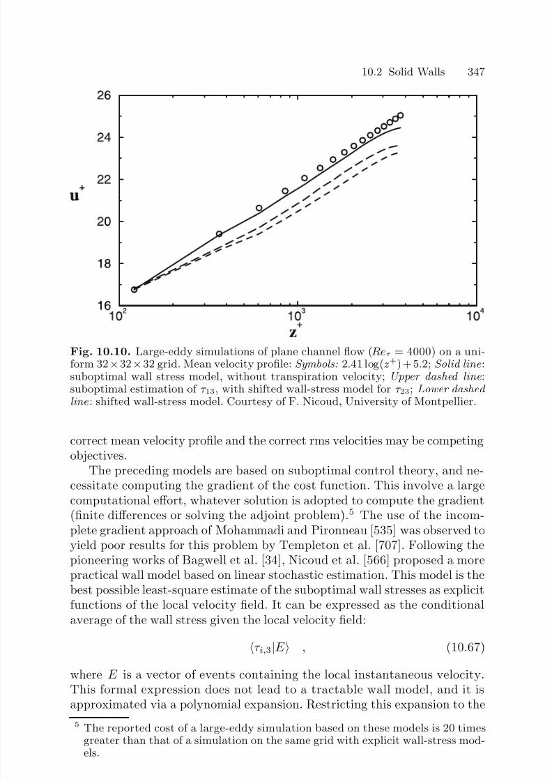
7/21/2019 Large Eddy Simulation for Incompressible Flows
http://slidepdf.com/reader/full/large-eddy-simulation-for-incompressible-flows 367/573
10.2 Solid Walls 347
Fig. 10.10. Large-eddy simulations of plane channel flow (Reτ = 4000) on a uni-form 32×32×32 grid. Mean velocity profile: Symbols: 2.41 log(z +) + 5.2; Solid line :suboptimal wall stress model, without transpiration velocity; Upper dashed line :suboptimal estimation of τ 13, with shifted wall-stress model for τ 23; Lower dashed line : shifted wall-stress model. Courtesy of F. Nicoud, University of Montpellier.
correct mean velocity profile and the correct rms velocities may be competingobjectives.
The preceding models are based on suboptimal control theory, and ne-cessitate computing the gradient of the cost function. This involve a largecomputational effort, whatever solution is adopted to compute the gradient(finite differences or solving the adjoint problem).5 The use of the incom-plete gradient approach of Mohammadi and Pironneau [535] was observed to
yield poor results for this problem by Templeton et al. [707]. Following thepioneering works of Bagwell et al. [34], Nicoud et al. [566] proposed a morepractical wall model based on linear stochastic estimation. This model is thebest possible least-square estimate of the suboptimal wall stresses as explicitfunctions of the local velocity field. It can be expressed as the conditionalaverage of the wall stress given the local velocity field:
τ i,3|E , (10.67)
where E is a vector of events containing the local instantaneous velocity.
This formal expression does not lead to a tractable wall model, and it isapproximated via a polynomial expansion. Restricting this expansion to the
5 The reported cost of a large-eddy simulation based on these models is 20 timesgreater than that of a simulation on the same grid with explicit wall-stress mod-els.

7/21/2019 Large Eddy Simulation for Incompressible Flows
http://slidepdf.com/reader/full/large-eddy-simulation-for-incompressible-flows 368/573
348 10. Boundary Conditions
Fig. 10.11. Large-eddy simulations of plane channel flow (Reτ = 4000) on a uni-form 32 × 32 × 32 grid. Shifted correlation model. Instantaneous isocontours of predicted stresses and velocity components at the first off-wall grid point. Courtesyof F. Nicoud, University of Montpellier.
first term, one obtains the following linear stochastic estimate for the wallstresses:
τ i,3|E ≈ LijE j , (10.68)
where the estimation coefficients Lij are governed by
τ i,3E k = LijE jE k . (10.69)
In practice, these coefficients are computed using reference data (directnumerical simulation data or suboptimal-control-based prediction of the wallstresses). The resulting model is an explicit model, whose cost is of the sameorder as those of the other explicit wall-stress models, which are able to re-
produce accurately the results of the suboptimally controlled simulations.Unfortunately, numerical experiments have shown this model to be very sen-sitive to numerical and modeling errors, indicating that it might be impossibleto find an accurate and robust6 linear wall stress model.6 A model whose accuracy will be the same whatever numerical method and sub-
grid model are employed.

7/21/2019 Large Eddy Simulation for Incompressible Flows
http://slidepdf.com/reader/full/large-eddy-simulation-for-incompressible-flows 369/573
10.2 Solid Walls 349
Fig. 10.12. Large-eddy simulations of plane channel flow (Reτ = 4000) on a uni-form 32 × 32 × 32 grid. Suboptimal prediction of the wall stresses, without transpi-ration velocity. Instantaneous isocontours of predicted stresses and velocity com-ponents at the first off-wall grid point. Courtesy of F. Nicoud, University of Mont-pellier.
Das–Moser Embedded Wall Model. In the case of an impermeable wall,the general equations (10.1) and (10.2) simplify to
∂ui∂t
+ ∂
∂xj(uiuj) +
∂p
∂xi− ν
∂
∂xj
∂ui∂xj
+ ∂uj∂xi
=
− ∂Ω
G(x − ξ)
p(ξ) − ν
∂ui∂xj
(ξ) + ∂uj∂xi
(ξ)
nj(ξ)dξ , (10.70)
∂ui∂xi
= 0 . (10.71)
The source term in the continuity equation cancels out, while the momen-tum source term is associated with the total force exerted on the wall. Whenfiltering through the wall, it is necessary to prolong the velocity field insidethe solid wall. This is done by assuming a zero velocity field inside the wallin a buffer zone Ω ∗.

7/21/2019 Large Eddy Simulation for Incompressible Flows
http://slidepdf.com/reader/full/large-eddy-simulation-for-incompressible-flows 370/573
350 10. Boundary Conditions
In the present formulation, the problem is to compute the source termin (10.70). Because the unfiltered velocity is set to zero in the wall, thewall stress is the surface forcing required to ensure that momentum is nottransfered to a buffer domain located inside the wall, i.e. that the velocity willremain zero. Using this remark, Das and Moser [164] suggested computingthe source term at each time step in order to minimize the transport of momentum from the fluid domain toward the buffer zone. The embedded wallboundary condition is then a control minimizing the following cost function:
J =
Ω∗
|u|2 + α
∂ u
∂t
2
dx , (10.72)
where the first term forces the energy in the buffer zone to be small, andthe second one ensures that the momentum transfer of energy across thewall surface is small. The constant α scales like ∆t2 in plane channel flowcomputation, with ∆t being the time step.
ODT-Based Wall Model. Structural models presented in Sect. 7.7 can beused to reconstruct subgrid fluctuations inside the first cell near the solidwalls. This strategy was adopted by Schmidt et al. [650], who used the ODT-based model (see p. 257) to predict the near wall dynamics, the outer part
of the boundary layer being computed using a classical large-eddy simula-tion method. It is worth noting that this approach is reminiscent of the oneproposed by Balaras based on thin boundary layer equations within the firstgrid cell.
The proposed coupling strategy, based on the existence of an overlapregion between ODT and large-eddy simulation (see p. 257 for a detaileddescription of the ODT-based model), is the following. This zonal decom-position is illustrated in Fig. 10.13. An ODT-type simulation is performedwithin the first grid cell of the large-eddy simulation grid. The large-eddysimulation provides the ODT with boundary conditions at the top of theODT domain, and also appears in the evaluation of the advection speed inthe ODT equation. The ODT simulation provides the large-eddy simulationwith subgrid fluxes in two different regions: (i) in the inner region (i.e. thefirst grid cell off the wall), the full fluxes appearing in the large-eddy simula-tion equations is computed using the ODT fluctuations and (ii) in the outer region , which has a thickness L (L being the maximum size for eddy eventsallowed in the ODT simulation within the inner region). In the outer region,ODT equations are not solved, but the influence of large events belongingto the ODT solution computed in the inner region is taken into account.
This is achieved by adding the contribution of ODT eddy events of sufficientsize to reach the considered position in the large-eddy simulation grid to theconventional fluxes in that region.

7/21/2019 Large Eddy Simulation for Incompressible Flows
http://slidepdf.com/reader/full/large-eddy-simulation-for-incompressible-flows 371/573
10.2 Solid Walls 351
Fig. 10.13. Schematic of the ODT-based wall model.
10.2.3 Wall Models: Achievements and Problems
Most of the wall models presented above have been developed on the grounds
of the dynamics of the zero-pressure gradient, equilibrium flate plate bound-ary layer. In practical cases, most of them exhibit the same behavior:
– In attached, equilibrium flows, satisfactory results (skin friction predictedwithin a 20% error) on the mean flow are recovered on medium grids, i.e.on grids such that the first cell off the wall has the following dimensions:
∆x+ ≤ 500, ∆y+ ≤ 200 − 300, ∆z+ = 50 − 150 .
On such a grid, spurious bumps are observed in the turbulence intensities
just near the first grid point (see Fig. 10.14). These unphysical overshootsare associated to the existence of large spurious streaky structures, whosesize can be governed by either the mesh size or the numerical and subgridmodel dissipation. The growth of these structures might be explained bythe same mechanisms as the physical streaky vortices: they might be partsof an autonomous self-sustaining cycle feeded by the mean shear involvinglow-/high-speed streaks and streamwise vortices. Another possible cause isthat they could arise from the splatting of turbulent eddies coming fromthe outer part of the boundary layer on the boundary condition (almost
all models account for the impermeability constraint enforcing a vanishingwall normal velocity).No general cure for this problem is known. These bumps can be dampedby scrambling the spurious streamwise vortices by adding a random noisein the region where they are detected [592]. Partial error cancellation whenusing a very dissipative subgrid model has also been observed: the spurious

7/21/2019 Large Eddy Simulation for Incompressible Flows
http://slidepdf.com/reader/full/large-eddy-simulation-for-incompressible-flows 372/573
352 10. Boundary Conditions
Fig. 10.14. Resolved Reynolds stresses in a plane channel flow with Grotzbach
wall stress model. Courtesy of Y. Benarafa and F. Ducros, CEA.
streaks are then damped. It was also shown by Nicoud that some controlon the turbulence intensities can be achieved playing of the wall stressesand the wall normal velocity, but with a higher error level on the mean flowprofile. It is worth noticing that the problem of the reduction of this erroris close to the one of the active control of the boundary layer dynamics.
– On very coarse grids, the models are no longer ables to yield an accurateprediction of the mean flow profile: the correct logarithmic slope is notrecovered in the logarithmic layer, the skin friction is poorly predicted (seeFig. 10.15), ... It must be observed that on very coarse grids the problemis much more complicated: (i) the near-wall layer dynamics is not resolved,(ii) large subgrid modeling errors occur in the core of the flow since a largepart of the turbulent kinetic energy is contained in subgrid scales (and mostsubgrid scale models are not good at taking into account a large part of thefull turbulent kinetic energy), and (iii) since the mesh is coarse, numericalerrors may become dominant.
– Most models are not very efficient at predicting separation, since they
are based on very stringent assumptions. This was observed, among otherstudies, by Temmerman et al. [706] in a wavy channel configuration wherethe location of the separation point (and therefore of the reattachmentpoint) is seen to be sensitive to the wall model. A noticeable exception isthe Thin Boundary Layer Model, which has been proved to yield a satisfac-

7/21/2019 Large Eddy Simulation for Incompressible Flows
http://slidepdf.com/reader/full/large-eddy-simulation-for-incompressible-flows 373/573
10.2 Solid Walls 353
Fig. 10.15. Error on the computed skin friction versus the size of the mesh in
the streamwise direction (in wall units) in plane channel flow computation, withdifferent wall models. Steady RANS solution is shown for comparison. Courtesy of Y. Benarafa and F. Ducros, CEA.
tory prediction of an incipient separated region on smooth airfoil trailingedge [754] and on a circular cylinder at high Reynolds number [113]. Inconfigurations where the separation point is imposed like in the backwardfacing step case investigated by Cabot [87], main features of the flow arerelatively insensitive to the way the solid wall is treated inside the sepa-
rated region. But skin friction in the seprated region is of course subject toconsequent errors. First trials for the definition of wall models devoted toseparated regions have been done [706, 370], but satisfactory results havenot yet been obtained. A main difficulty is the lack of universal scaling lawfor the mean velocity profile in separated flows.
– Some wall-stress models require values related to the mean flow as inputs.This need lead to a severe limitation of the models, since the mean flowmust be known, or some homogeneous directions must exists to enablethe evaluation of some statistiscal moments of the instantaneous fields at
each time step. Possible solutions to overcome this problem are: (i) torun several statistically equivalent simulations in parallel and to performtrue statistical average or (ii) to use a local spatial averaging instead of a statistical average. The latter solution is used by Hassan and Barsamian[298] to obtain a localized version of the Grotzbach model.

7/21/2019 Large Eddy Simulation for Incompressible Flows
http://slidepdf.com/reader/full/large-eddy-simulation-for-incompressible-flows 374/573
354 10. Boundary Conditions
10.3 Case of the Inflow Conditions
10.3.1 Required Conditions
Representing the flow upstream of the computational domain also raises dif-ficulties when this flow is not fully known deterministically, because the lackof information introduces sources of error. This situation is encountered fortransitional or turbulent flows that generally contain a very large number of space–time modes [631]. Several boundary condition generation techniquesare used for furnishing information about all the modes contained to thelarge-eddy simulation computation.
Apart the purely mathematical problem of defining well-posed inflow
boundary conditions, the Large-Eddy Simulation and the Direct Numeri-cal Simulation techniques raise the problem of reconstructing the turbulentfluctuations at the inlet plane in an accurate way. The exact definition of accurate turbulent inflow conditions is still an open question, but the accum-lulated experience proves that both kinetic energy and coherence of the inletfluctuations must be taken into account to minimize the size of the bufferregion that exists downstream the inlet plane, in which turbulent fluctua-tions consistent with the Navier–Stokes dynamics are reconstructed by thenon-linear effects. This need is illustrated in Fig. 10.16, which displays results
obtained in Direct Numerical Simulation of a two-dimensional mixing layer.
10.3.2 Inflow Condition Generation Techniques
Stochastic Recontruction from a Statistical One-Point Description.When the freestream flow is described statistically (usually the mean velocityfield and the one-point second-order moments), the deterministic informationis definitively lost. The solution is then to generate instantaneous realizationsthat are statistically equivalent to the freestream flow, i.e. that have the same
statistical moments.In practice, this is done by superimposing random noises having the same
statistical moments as the velocity fluctuations, on the mean statistical pro-file. This is expressed as
u(x0, t) = U (x0) + u(x0, t) , (10.73)
where the mean field U is given by experiment, theory or steady computa-tions, and where the fluctuation u is generated from random numbers. This
technique makes it possible to remain in keeping with the energy level of thefluctuations as well as the one-point correlations (Reynolds stresses) in thedirections of statistical homogeneity of the solution, but does not reproducethe two-point (and two-time) space–time correlations [432, 540, 493]. Theinformation concerning the phase is lost, which can have very harmful conse-quences when the consistency of the fluctuations is important, as is the case

7/21/2019 Large Eddy Simulation for Incompressible Flows
http://slidepdf.com/reader/full/large-eddy-simulation-for-incompressible-flows 375/573
10.3 Case of the Inflow Conditions 355
Fig. 10.16. Illustration of the influence of the turbulent inlet boundary condition(DNS of a 2D mixing layer). Iso-contours of instantaneous vorticity are shown.Top: reference 2D simulation. Below: Truncated simulation using as inflow con-ditions: a) exact instantaneous velocity field stored at the x0 section; b) randomvelocity fluctuations spatially and temporally uncorrelated (white noise) having the
same Reynolds stress tensor components as in case (a); c) instantaneous velocityfield preserving temporal two point correlation tensor of case (a); d) instantaneousvelocity field preserving spatial two point correlation tensor of case (a); e) recon-structed velocity field with the aid of Linear Stochastic Estimation procedure fromthe knowledge of exact instantaneous velocity field at 3 reference locations (centerof the mixing layer and ±δ ω/2 where δ ω is the local vorticity thickness). Courtesyof Ph. Druault and J.P. Bonnet, LEA.
7/21/2019 Large Eddy Simulation for Incompressible Flows
http://slidepdf.com/reader/full/large-eddy-simulation-for-incompressible-flows 376/573
356 10. Boundary Conditions
for shear flows (mixing layer, jet, boundary layer, and so forth). That is, thecomputations performed show the existence of a region in the computationaldomain in which the solution regenerates the space–time consistency specificto the Navier–Stokes equations [139]. The solution is not usable in this re-gion, which can cover a large part7 of the computational domain, and thisentails an excess cost for the simulation. Also, it appears that this techniqueprevents the precise control of the dynamics of the solution, in the sense thatit is very difficult to reproduce a particular solution for a given geometry.
A few ways to generate the random part of the inlet flow are now pre-sented:
1. The Lee–Lele–Moin procedure (p. 356).
2. The Smirnov–Shi–Celik procedure and Batten’s simplified version(p. 356).3. The Li–Wang procedure (p. 358).4. The Weighted Amplitude Wave Superposition procedure (p. 358).5. The digital filter based method (p. 359).6. The Arad procedure (p. 360).7. The Yao–Sandham model (p. 361).
The LLM Procedure. The first method was proposed by Lee, Lele andMoin [432] for a flow evolving in the direction x and homogeneous in the
two other directions, and statistically stationary in time. Assuming that theenergy spectrum of a flow variable φ, E φφ, is prescribed in terms of frequencyand two transverse wave numbers, the Fourier coefficients of the fluctuatingpart of φ are prescribed as
φ(ky, kz, ω , t) =
E φφ(ky, kz, ω) exp [ıψr(ky, kz, ω , t)] , (10.74)
where ψr is the phase factor and ı =√ −1. The dependence of this phase
factor on time and transverse wave numbers is necessary so that the signal
generated is not periodic. The authors propose changing ψr only once ina given time interval T r at a random instance by a random bounded amount∆ψr. The resulting signal is not continuous, and the frequency spectrum of the generated turbulence is not equal to E φφ.
The authors get satisfactory results for decaying isotropic turbulence byapplying this procedure to each fluctuating velocity component ui, but itsapplication to advanced transitional flows or turbulent flows yields the oc-currence of large non-physical transition regions.
The SSC Procedure. Another procedure was proposed by Smirnov, Shi andCelik [677] with application to wall-bounded flows. It involves scaling andorthogonal transformation operations applied to a continuous field generatedas a superposition of harmonic functions.
7 Numerical experiments show that this region can cover more than 50% of thetotal number of simulation points.

7/21/2019 Large Eddy Simulation for Incompressible Flows
http://slidepdf.com/reader/full/large-eddy-simulation-for-incompressible-flows 377/573
10.3 Case of the Inflow Conditions 357
Let Rij = uiuj be the (anisotropic) velocity correlation tensor at the
inlet plane (see Appendix A for a precise definition). The first step of theSSC procedure consists of finding an orthogonal transformation tensor Aijthat would diagonalize Rij (without summation over Greek indices)
AαiAβjRij = δ αβλ2β , (10.75)
AikAkj = δ ij , (10.76)
where the coefficients λ1, λ2 and λ3 play the role of turbulent fluctuatingvelocities u1, u2 and u3 in the new coordinate system. It is worth noting thatboth the transformation matrix and new coefficients are functions of space.
The second step consists of generating a transient flow-field V in a three-dimensional domain and rescaling it. This field is computed using the modi-fied Kraichnan’s method:
V i(x, t) =
2
N
N n=1
ani cos(knj xj + ωnt) + bni sin(knj xj + ωnt)
, (10.77)
with
xj = xjL0
, t = t
T 0, c =
L0
T 0, knj = knj
c
λj, (10.78)
ani = ijmζ nj knm, bni = ijkξ nj k
nm , (10.79)
ζ n
j , ξ n
j , ωn ∈ N (0, 1), kn
i ∈ N (0, 1/2) , (10.80)where L0 and T 0 are the length- and timescales of turbulence, ijm is thepermutation tensor, and N (M, σ) is a normal distribution with mean M and standard deviation σ. Quantities ωn and knj represent a sample of nfrequencies and wave number vectors of the turbulent spectrum. In practice,the authors use the following model spectrum:
E (k) = 16
2
πk4 exp(−2k2) . (10.81)
The last step consists of applying scaling and orthogonal transformationsto V to recover the synthetic fluctuating field in physical space:
W α = λαV α, ui = AikW k . (10.82)
The resulting fluctuating field is nearly divergence-free, and has corre-lation scales L0 and T 0 with the correlation tensor Rij . This method wassuccessfully applied to boundary-layer flows.
A simplified formulation is proposed by Batten et al. [49], which doesnot require the use of the orthogonal transformation. This simplification isachieved redefining the parameters λj as
λj =
3Rlmkjl kjm
2kjnkjn, (10.83)
and using the relation (10.77) to prescribe directly the velocity fluctuationsu instead of V .

7/21/2019 Large Eddy Simulation for Incompressible Flows
http://slidepdf.com/reader/full/large-eddy-simulation-for-incompressible-flows 378/573
358 10. Boundary Conditions
The Li–Wang Procedure. Another random generation technique for fluctua-tions in a boundary-layer flow was proposed by Li and Wang [446]. Fluctua-tions are reconstructed using the following equation:
u(x,y,z, 0) =√
2
N 1l=1
N 2m=1
N 3n=1
E u(ωxl, ωym, ωzn)∆ωx∆ωy∆ωz
× cos(ωxlx + ωy
my + ωznz + φlmn) , (10.84)
where E u is the target spectrum, φlmn a random phase with uniform distri-bution, and ωxl = (l − 1)∆ωx the angular frequency in the x direction. Theperiodicity is eliminated by defining
ωxl = ωxl + δωx , (10.85)
where δωx is a small random frequency. The time-evolving fluctuating fieldat the inlet plane is then reconstructed using Taylor’s frozen turbulence hy-pothesis:
u(0, y , z , t) = u(x, y , z , 0), x = U ct , (10.86)
where U c is an advecting velocity.
Weighted Amplitude Wave Superposition (WAWS) spectral representation method. Another procedure relying on modified random time series to gen-erate velocity fluctuations was proposed by Glaze and Frankel [265]. Thismethod, referred to as the WAWS method, is capable of simulating bothspatial and temporal correlation. It is based on the regeneration of the fluc-tuating signal from its cross-spectral density at the inlet plane. As a result,both spatial correlation across the inlet plane and the power spectrum of eachvelocity component can be enforced.
Let M and N be the number of grid points at the inlet plane and the
number of frequencies to be prescribed, respectively. Each velocity componentis synthetized at the ith grid point using the following relation
ui(t) =√
2i
m=1
N n=1
|H im(ωn)|
2∆ω cos(ωnt + θim(ωn) + φmn) , (10.87)
with
ωn =
n − 1
2∆ω, ωn = ωn + δωn , (10.88)
where ∆ω = ωu/N , ωu and δωn ∈ [−∆ω/20, +∆ω/20] are the frequencyresolution, the maximum frequency and a small random perturbation, re-spectively. The parameters φmn are random phases perturbations uniformlydistributed between 0 and 2π. The key parameters are the components of the transfer function matrix, H im(ωn), which are linked to the cross spectral

7/21/2019 Large Eddy Simulation for Incompressible Flows
http://slidepdf.com/reader/full/large-eddy-simulation-for-incompressible-flows 379/573
10.3 Case of the Inflow Conditions 359
density matrix components S ij(ωn) through the relation
S ij(ωn) = H ik(ωn)H ∗kj(ωn) (10.89)
where H ∗ is the Hermitian transpose of H . Since the H matrix is not uniquefor a given S , a method should be chosen to compute it. Glaze and Frankelused a Cholesky decomposition to obtain a lower-triangular matrix, leadingto simple calculations. The θim(ωn) parameter in (10.87) are defined writingthe transfer function matrix components in polar form:
H im(ωn) = |H im(ωn)|eıθim(ωn) . (10.90)
Since the foreknowledge of the cross-spectral density matrix S for eachvelocity component is not a realistic requirement in practice, the next stepconsists in modeling it from available data. Noticing that it can be expressedas a function of one-point spectral density and the complex coherence functionγ im:
S im(ωn) = γ im
S ii(ωn)S mm(ωn) , (10.91)
the problem is equivalent to prescribing the power spectrum at each grid pointand the coherence function. This is achieved using informations available oneach flow.
The case of the near-field of a turbulent jet studied in [265] is given belowas an illustration. The coherence function is estimated like follows
γ im = exp
−A(rim + Br2
im)
U im
, A = 1, B = 4 , (10.92)
where rim is the distance between points i and m and U im is the averagemean velocity between these points. The power spectrum is obtained usingthe von Karman model:
S ii(f ) = 4 f (u
)2
f (1 + 70.8f 2)5/6, (10.93)
where u is the rms turbulence intensity, f the frequency (in hertz), f =Luf /U the associated Strouhal number, with U the mean velocity and Luthe turbulent integral scale.
Digital Filter Based Method. Klein, Sadiki and Janicka [396] introduceda new approach based on signal modeling through the use of linear non-recursive filters. The general form of the discrete time series for the u velocitycomponent at any grid point of the inflow plane is
um =N
n=−N
bnrm+n , (10.94)

7/21/2019 Large Eddy Simulation for Incompressible Flows
http://slidepdf.com/reader/full/large-eddy-simulation-for-incompressible-flows 380/573
360 10. Boundary Conditions
where rm is a series of random data with zero mean and such that rmrn =δ mn and bn are the digital filter coefficients. The autocorrelation of the syn-thetized signal is
umum+kumum =
N j=−N +k bjbj+kN
j=−N b2j
. (10.95)
The problem consists in inverting this relation to compute the coefficientsof the digital filter associated to a given autocorrelation tensor. The authorspropose to use a model autocorrelation function to obtain a simple form of the filter coefficients. They use the following form, which is valid for fullydeveloped homogeneous turbulence (autocorrelation of the u component inthe direction associated to it):
Ruu(r, 0, 0) = exp
πr2
4L2
, (10.96)
where L is a prescribed integral length scale. Combining this model autocor-relation function with relation (10.95) and setting L = n∆x, one obtains
N j=−N +k bjbj+kN
j=−N b2j = exp−
π(k∆x)2
4(n∆x)2 = exp−πk2
4n2 , (10.97)
whose accurate approximate explicit solution is
bk = ak N j=−N a
2k
, ak = exp
−πk2
4n2
. (10.98)
This method yields the generation of a set of values with the targetedautocorrelation. Cross-correlations between velocity component can be en-
forced using the same change of variable as in the SSC procedure. Extensionto the three-dimensional case straightforward, applying the procedure in se-quentially in the three directions. This method was shown to give satifactoryresults in plane jet simulations.
Arad’s Procedure. Arad [16] proposed a reconstruction technique for an initialcondition based on physical observations related to the turbulence productionprocess in a boundary layer. Assuming a general form of the perturbationcorresponding to linearly unstable modes of the mean profile,
ui(x, y, z, t) = ui(z)exp(ı(αx + βy − ωt)), ui(z) = Aiφ exp(−γz2) ,(10.99)
where Ai is the amplitude of the mode and φ a random number. This ideaof Arad is to design the fluctuations so that their growth rate will be maxi-mized, resulting in a short unphysical transient region near the inlet plane.
7/21/2019 Large Eddy Simulation for Incompressible Flows
http://slidepdf.com/reader/full/large-eddy-simulation-for-incompressible-flows 381/573
10.3 Case of the Inflow Conditions 361
Remarking that in a boundary layer the turbulence production term has thefollowing form
P = uw
u2τ
dU +
dz+ , (10.100)
and taking into account the fact that quadrant Q2 (ejection: u < 0, w > 0)and Q4 (sweep: u > 0, w < 0) events have a dominant contribution to theshear stress uw, Arad proposed introducing a phase shift between u andw:
u(x, y, z, t) = u(z) cos(αx + βy − ωt) , (10.101)
w(x, y, z, t) = u(z) cos(αx + βy − ωt + π) . (10.102)
The spanwise component fluctuation, v, is assumed to be in phase with u
in Arad’s work. The resulting fluctuations correspond to sweep and ejectionevents.
The Yao–Sandham Procedure. A more sophisticated procedure was proposedby Yao and Sandham [781, 644], which relies on the observations that fluc-tuations in the inner and outer parts of the boundary layer have differentcharacteristic scales. As a consequence, specific disturbances are introducedin each part of the boundary layer. The inner-part fluctuations, uinner are
designed to represent lifted streaks with an energy maximum at z+ p,j :
uinneri (y , z , t) = cij exp(−z+/z+
p,j) sin(ωjt)cos(ky,jy + φj) . (10.103)
The outer-part fluctuation is assumed to be of the following form (witha peak at z p,j)
uouteri (y , z , t) = cij
z
z p,jexp(−z/z p,j) sin(ωjt)cos(ky,jy + φj) , (10.104)
where subscripts i = 1, 2 and j are related to the velocity component andto the mode indices, respectively, and cij are constants. The + superscriptrefers to inner coordinates (wall units). The φj are phase shifts, ωj are forcingfrequencies, and ky,j are spanwise wave numbers. These parameters are to beadjusted using information on the boundary-layer dynamics. The spanwisevelocity component is deduced from the continuity constraint.
In the inner region of the boundary layer, it is assumed that the distur-bances travel downstream for a distance of 1000 wall units at a convectivevelocity U c ≈ 10 uτ , where uτ is the friction velocity within a time period.
The wave numbers ky,j are chosen such that there will be four streaks witha typical characteristic length of 100 wall units.In the outer region, the downstream travelling distance is taken equal to
16 and the convection velocity is U c ≈ 0.75 U ∞, where U ∞ is the external ve-locity. The spanwise wave number is chosen to be of the order of the spanwiseextent of the computational domain.

7/21/2019 Large Eddy Simulation for Incompressible Flows
http://slidepdf.com/reader/full/large-eddy-simulation-for-incompressible-flows 382/573
362 10. Boundary Conditions
Yao and Sandham applied this procedure to a turbulent boundary layer,taking one mode in the inner region and three in the outer region. Corre-sponding parameters are given in Table 10.1. They also add a random noisewith a maximum amplitude of 4% of the external velocity to prevent possiblespurious symmetries.
Table 10.1. Coefficients of the four-mode Yao–Sandham model of fluctuations forboundary-layers.
j c1j c2j ωj ky,j φj z +p,j z p,j
inner region 0 0.1 −0.0016 0.1 π 0. 12 −outer region 1 0.3 −0.06 0.25 0.75π 0. − 1.outer region 2 0.3 −0.06 0.125 0.5π 0.1 − 1.5outer region 3 0.3 −0.06 0.0625 0.25π 0.15 − 2.0
Deterministic Computation.
Precursor Simulation. One way of minimizing the errors is to perform a sim-ulation of the upstream flow [740, 226, 649], called a precursor simulation,
with a degree of resolution equivalent to that desired for the final simulation(see Fig. 10.17). This technique almost completely eliminates the errors en-countered before, and offers very good results. On the other hand, it is hardlypractical in the general case because it requires reproducing the entire history
Fig. 10.17. Schematic of the precursor simulation technique. A precursor sim-ulation of an attached boundary layer flow is performed. An extraction plane isdefined, whose data are used as an inlet boundary condition for a simulation of theflow past a trailing edge.
7/21/2019 Large Eddy Simulation for Incompressible Flows
http://slidepdf.com/reader/full/large-eddy-simulation-for-incompressible-flows 383/573
10.3 Case of the Inflow Conditions 363
of the flow which, for complex configurations, implies very high computationcosts. Another problem stemming from this approach is that of causality:since the precursor is computed separately, no feedback of information fromthe second simulation is possible. This is a one-way coupling between twosimulations that can become problematic when a signal (acoustic wave, forexample) is emitted by the second.
Li et al. [445] reduced the cost of the precursor technique by storing theresults of the precursor simulation over a (relatively) short time, and cyclingin time over these data to generate the flow at the inlet plane of the maincomputation. In practice, the precursor results are stored over a time of theorder of the integral timescale of the flow, and windowed to get a periodicsignal. This technique has been applied to a plane mixing layer flow. Numer-
ical results show that non-linear interactions quickly eliminate the spuriousperiodicity imposed at the inlet plane (about 25% of the total computationaldomain is contaminated). The efficiency of the method for flows with lowerscrambling effects, such as wall-bounded flows, remains to be investigated.
Lund’s Extraction/Rescaling Technique. Lund et al. [463] developed a variantof the precursor approach for boundary layers, in which the information atthe inlet plane is produced from that contained in the computation. Thereis no longer any need for a precursor. The heart of the method is a means of
estimating the velocity at the inlet plane, based on the velocity field extractedfrom the simulation on a plane downstream, as illustrated in Fig. 10.18.The main difficulty arises from the fact that the mean flow is not parallel,
i.e. the boundary layer thickness increases, and the flow at the extractionplane must first be rescaled before being used at the inlet plane.
The first step consists of decomposing the extracted flow, ue(x, t), as thesum of a mean and a fluctuating part:
uei (x, y, z, t) = ue
i (x, y, z, t) + U ei (y, z) . (10.105)
The second step consists of rescaling the mean flow part using classicalscalings related to the mean velocity profile of the turbulent boundary layer(see Sect. 10.2.1). In practice, the rescaling is carried out according to thelaw of the wall in the inner region and the defect law in the outer regionof the boundary layer, leading to the following relations for the streamwisecomponent:
U inner = uτ (x)f 1(z+) , (10.106)
U ∞ − U
outer
= uτ (x)f 2(η) , (10.107)
where x is assumed to be the streamwise direction, z the wall-normal direc-tion, U ∞ the external velocity, uτ the friction velocity, η = z/δ the outer coor-dinate, δ the boundary-layer thickness, and f 1 and f 2 two universal functionsto be determined. These two scaling laws dictate that the extracted mean

7/21/2019 Large Eddy Simulation for Incompressible Flows
http://slidepdf.com/reader/full/large-eddy-simulation-for-incompressible-flows 384/573
364 10. Boundary Conditions
Fig. 10.18. Schematic of Lund’s extraction/rescaling technique. Instantaneous
isolevels of streamwise velocity in a boundary layer are shown. Courtesy of E. Tromeur and E. Garnier, ONERA.
velocity U e and the rescaled mean velocity at the inflow, U r, are related inthe inner and outer regions via
U r,inner = γU e(z+,r) , (10.108)
U r,outer = γU e(ηr) + (1− γ )U ∞ , (10.109)
with
γ = ur
τ
ueτ
, (10.110)
and where urτ and ue
τ are skin friction at the inlet plane and extraction plane,respectively, z+,r is the inner coordinate computed at the inlet plane, and ηr
is the external coordinate computed at the inlet plane. A linear interpolationis used between the grid points of the planes.
A similar technique is used to rescale the mean wall-normal component,
yielding:
W r,inner = W e(z+,r) , (10.111)
W r,outer = W e(ηr) . (10.112)
7/21/2019 Large Eddy Simulation for Incompressible Flows
http://slidepdf.com/reader/full/large-eddy-simulation-for-incompressible-flows 385/573
10.3 Case of the Inflow Conditions 365
The third step consists of rescaling the fluctuating part of the instanta-neous field:
u,r,inneri = γu,e(y, z+,r, t) , (10.113)
u,r,outeri = γu,e(y, ηr, t) . (10.114)
The last step consists of writing a composite profile for the full instan-taneous velocity at the inlet plane, ur, that is approximately valid over theentire boundary layer. It is defined as a weighted average of the inner andouter profiles
uri = U r,inneri + u
,r,inneri (1 − β (ηr))
+
U r,outeri + u,r,outer
i
β (ηr) , (10.115)
with
β (η) = 1
2
1 + tanh
α(η − b)
(1 − 2b)η + b
/tanh(α)
, (10.116)
where α = 4 and β = 0.2.This extraction/rescaling technique is observed to be efficient in practice,
but must be used with care. The first point is that the extraction plane mustbe located far enough from the inlet to prevent spurious couplings in thecomputed solution. This constraint is satisfied by taking a distance betweenthe two planes larger than the correlation length of the fluctuations in thestreamwise direction. The second point is that it is valid for fully turbulentself-similar boundary layers only, and that the scaling laws must hold toobtain a relevant procedure.
Spille-Kohoff–Kaltenbach Method. The extraction/rescaling technique pre-sented above suffers some lack of generality, because it relies on self-similarityassumptions and can introduce some spurious couplings inside the computa-tional domain. A more general method was proposed by Spille-Kohoff andKaltenbach [686], with application to a boundary-layer.
The core of the method is the definition of a buffer region, referred toas the control region, near the inlet plane, where a body force is adjustedin order to recover targeted profiles of turbulent fluctuations at a positionlocated downstream of this buffer region. The body force is defined within
the closed-loop control theory, and makes it possible, at least theoretically,to control both rms profiles and integral properties of the boundary layer.This procedure is illustrated in Fig. 10.19.
A random fluctuation is first specified at the inlet plane, together witha mean velocity profile. The body force is applied to the wall-normal velocitycomponent only. The rationale for this is the observation that −wwdU/dz

7/21/2019 Large Eddy Simulation for Incompressible Flows
http://slidepdf.com/reader/full/large-eddy-simulation-for-incompressible-flows 386/573
366 10. Boundary Conditions
Fig. 10.19. Schematic of the Spille-Kohoff–Kaltenbach method. Courtesy of H. Kaltenbach, University of Berlin.
is the dominant production term in the balance equation for the shear stress−uw. The amplitude of the body force at a streamwise position x0 isadjusted via a PI controller in order to achieve a prescribed shear–stressprofile −uwtarget. This target can be defined using experimental data orRANS simulations. Another way to define the targeted profile is to extractand rescale it from a position xR downstream of the control region.8
The instantaneous body force in the plane x = x0 is computed as follows
f (x0, y , z , t) = A(z, t) [u(x0, y , z , t) − uy,t(x0, z)] , (10.117)
8 It is important to remark that only mean profiles are extracted, and not instan-taneous fields as in Lund’s approach. This prevents the occurrence of spuriousfeedback.
7/21/2019 Large Eddy Simulation for Incompressible Flows
http://slidepdf.com/reader/full/large-eddy-simulation-for-incompressible-flows 387/573
10.3 Case of the Inflow Conditions 367
where the amplitude A(z, t) is given by
A(z, t) = αe(z, t) + β t0 e(z, t
)dt
, (10.118)
where α and β are two arbitrary parameters. The averaging operator y,tis associated with the average in the spanwise (homogeneous) direction andin time over a sliding window of width equal to O(10)δ/U ∞. The error terme(z, t) is a measure of the difference between the computed and the prescribedshear stress:
e(z, t) = uwtarget(x0, z) − uwy,t(x0, z , t) . (10.119)
In order to prevent unphysically large values of the shear stress, the bodyforce is applied only at grid points satisfying the following four instantaneousconstraints:
|u| < 0.6 U ∞, |w| < 0.4 U ∞, uw < 0, |uw| > 0.0015 U 2∞ .(10.120)
If the extraction technique is used to specify target values inside the con-trol region, another closed-loop controller is used to control the boundary-layer thickness at the inlet plane until the target value is obtained at the
extraction plane. Similarly, the wall-normal velocity component at the top of the computational domain is controlled in order to obtain the desired stream-wise pressure gradient. In this case, the authors observed that the adjustmenttime for reaching statistically steady values is of the order of 100 δ/U ∞.
Semideterministic Recontruction. Bonnet et al. [64, 199] propose anintermediate approach between the two previous ones, to recover the two-point correlations of the inflow with no preliminary computations. The signalat the inflow plane is decomposed in the form
u(x0, t) = U (x0) + U c(x0, t) + u(x0, t) , (10.121)
where U (x0) is the mean field, U c(x0, t) the coherent part of turbulent fluc-tuations, and u(x0, t) the random part of these fluctuations. In practice, thislast part is generated by means of random variables and the coherent partis provided by a dynamical system with a low number of degrees of freedom(like the POD, as seen in the Introduction), or by linear stochastic estimation,which gives access to the two-point correlations.

7/21/2019 Large Eddy Simulation for Incompressible Flows
http://slidepdf.com/reader/full/large-eddy-simulation-for-incompressible-flows 388/573
11. Coupling Large-Eddy Simulationwith Multiresolution/Multidomain Techniques
11.1 Statement of the Problem
This chapter is devoted to the presentation of the coupling of large-eddysimulation with multiresolution and/or multidomain approaches. The mainpurpose of these couplings is to decrease the computational cost of the large-eddy simulations by clustering the degrees of freedom in regions of interest.The key idea is to adapt locally the cutoff length scale of the simulation, i.e.to refine the computational grid.1 This grid refinement is associated with thedefinition of different subdomains with varying resolution.2
The methods proposed by various research groups can be classified asfollows:
– Methods relying on fully overlapping subdomains (Sect. 11.2), as shownin Fig. 11.1. The term fully overlapping means here that the subdomainwith the finest resolution is totally embedded within the coarsest resolutionsubdomain.
Fig. 11.1. Multiresolution decomposition with full overlap.
1 This corresponds to h-adaptivity within the framework of h– p methods. We willfocus on h-adaptivity only, because these are the most employed methods, evenwithin the finite-element framework.
2 The problem of mesh adaptation on unstructured grids for large-eddy simulationwill not be discussed here, because it has not yet been treated.
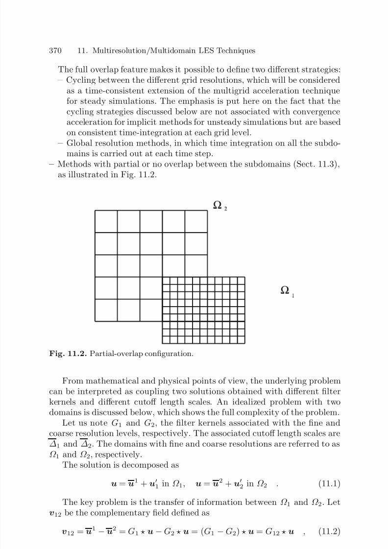
7/21/2019 Large Eddy Simulation for Incompressible Flows
http://slidepdf.com/reader/full/large-eddy-simulation-for-incompressible-flows 389/573
370 11. Multiresolution/Multidomain LES Techniques
The full overlap feature makes it possible to define two different strategies:– Cycling between the different grid resolutions, which will be considered
as a time-consistent extension of the multigrid acceleration techniquefor steady simulations. The emphasis is put here on the fact that thecycling strategies discussed below are not associated with convergenceacceleration for implicit methods for unsteady simulations but are basedon consistent time-integration at each grid level.
– Global resolution methods, in which time integration on all the subdo-mains is carried out at each time step.
– Methods with partial or no overlap between the subdomains (Sect. 11.3),as illustrated in Fig. 11.2.
Fig. 11.2. Partial-overlap configuration.
From mathematical and physical points of view, the underlying problemcan be interpreted as coupling two solutions obtained with different filterkernels and different cutoff length scales. An idealized problem with twodomains is discussed below, which shows the full complexity of the problem.
Let us note G1 and G2, the filter kernels associated with the fine andcoarse resolution levels, respectively. The associated cutoff length scales are∆1 and ∆2. The domains with fine and coarse resolutions are referred to asΩ 1 and Ω 2, respectively.
The solution is decomposed as
u = u1 + u1 in Ω 1, u = u2 + u2 in Ω 2 . (11.1)
The key problem is the transfer of information between Ω 1 and Ω 2. Letv12 be the complementary field defined as
v12 = u1 − u2 = G1 u−G2 u = (G1 −G2) u = G12 u , (11.2)

7/21/2019 Large Eddy Simulation for Incompressible Flows
http://slidepdf.com/reader/full/large-eddy-simulation-for-incompressible-flows 390/573
11.2 Methods with Full Overlap 371
where G12 is the restriction operator governing the transfer from the fine tothe coarse resolution level.
The problem of interfacing the two domains is thus the following:
– Transfer from Ω 1 to Ω 2: restrict u1 on Ω 2, or equivalently substract v12
from u1. This corresponds to the definition of the new filtering operatorG2
1 such thatG2 u = G2
1 G1 u . (11.3)
– Transfer from Ω 2 to Ω 1: defilter u2 at the ∆1 level, or equivalently addv12 to u2.
It is worth noting that most methods presented in this chapter can be
defined as static methods, because the number of levels of resolution is arbi-trarily fixed before the computation. Results dealing with dynamic methods,in which the number of levels is not fixed but automatically adjusted, arevery rare. Most advanced results dealing with the coupling of large-eddy sim-ulation with Adaptive Mesh Refinement (AMR) are given in Sect. 11.4.
11.2 Methods with Full Overlap
According to the notation used in the previous section, the full overlap cor-responds to Ω 1 ∩ Ω 2 = Ω 1.
The methods described in this section are:
– Methods with separate time-integration at each level. These methods aretrue multidomain methods, in the sense that the solution is integratedseparately on each subdomain. The solutions are coupled via informationtransfer from time to time. The methods presented below are:
1. The one-way coupling procedure of Khanna and Brasseur (Sect. 11.2.1).This method is the simplest one, and represents the minimal degreeof coupling between the two domains, the coarse level solution beingindependent of the fine level solution.
2. The two-way coupling procedure of Sullivan et al. (Sect. 11.2.2). Thismethod can be seen as an extension of the previous one, because theinformation transfer is now taken into account in both ways: from fineto coarse level, and from coarse to fine level.
3. The multilevel of Terracol et al. (Sect. 11.2.3), which is the most completeone. It relies on a two-way coupling, and also incorporates a dynamiccycling strategy. It is also the only one to incorporate a specific subgrid
modeling for multilevel computations.3
– Methods with a single time-integration step. These methods are not truemultidomain techniques, but rather multiblock methods. Time-integration
3 This multilevel method is an extension of the multilevel closure presented inSect. 7.7.7 (p. 271).
7/21/2019 Large Eddy Simulation for Incompressible Flows
http://slidepdf.com/reader/full/large-eddy-simulation-for-incompressible-flows 391/573
372 11. Multiresolution/Multidomain LES Techniques
is carried out at the same time at each level, without any distinctionbetween the different resolution levels. The example given below is themethod proposed by Kravchenko et al. (Sect. 11.2.4), which is based ona Galerkin method with overlapping trial functions.
11.2.1 One-Way Coupling Algorithm
Khanna and Brasseur [365] developed a one-way coupling embedded gridtechnique for large-eddy simulation of atmospheric boundary layers. The fineresolution (i.e. fine grid) domain Ω 1 is located in the near-wall region, inorder to permit a more accurate capture of details of the flow in that zone.The coarse resolution domain is noted Ω 2.
The solution is integrated in each domain independently for an arbitrarytime. The coupling is enforced by imposing boundary conditions on Ω 1 usingdata coming from the coarse solution Ω 2.
The proposed boundary conditions are the following:
– Dirichlet conditions on the velocity components:
u1∂Ω1
= u2∂Ω1
+ v12 , (11.4)
where the coarse resolution field u2 is obtained on the boundary of Ω 1, ∂Ω 1by a simple linear interpolation procedure. The complementary field v12
defined by relation (11.2) is here approximated by adding random noise per-turbation following a k−5/3 law within the spectral band k ∈ [π/∆2,π/∆1].
– Rescaling of the subgrid viscosity. The second boundary condition is ap-plied to the subgrid viscosity, which is rescaled in order to take into accountthe grid refinement. Assuming that both cutoffs are within the inertial sub-range, (5.36) leads to the following rescaling law for the subgrid viscosityat the boundary
ν 1sgs∂Ω1
=∆1
∆24/3
ν 2sgs∂Ω1
, (11.5)
where ν 1sgs and ν 2sgs are the values of the subgrid viscosity in Ω 1 and Ω 2,respectively.
In practice, the coupling is operated at the end of each time step.
11.2.2 Two-Way Coupling Algorithm
A two-way coupling procedure was proposed by Sullivan, McWilliams andMoeng [698] (also used in [62]). These authors consider a set of nested gridswith increasing resolution for simulating the planetary boundary layer. Thepresentation of the method is restricted to a two-grid case for the sake of simplicity. The extension to an arbitrary number of grids is straightforward.

7/21/2019 Large Eddy Simulation for Incompressible Flows
http://slidepdf.com/reader/full/large-eddy-simulation-for-incompressible-flows 392/573
11.2 Methods with Full Overlap 373
The coupling is achieved at each time step in the following way:
– From the coarse resolution level to the fine resolution level: boundary con-
ditions on ∂Ω 1 are obtained by interpolating the low-resolution field u2
(see (11.4)). The difference between this and the one-way coupling algo-rithm presented above is that the complementary field v12 is now neglected.
– From the fine resolution level to the coarse resolution level: the numericalfluxes at the coarse resolution level are computed by filtering the fluxescomputed at the fine resolution level on the overlap region. This can bewritten as follows:
∂ u2
∂t + G2
1 NS (u1) = 0, in Ω 1 ∩ Ω 2 , (11.6)
where NS denotes the Navier–Stokes operator. Another possibility, as pro-posed by Manhart and Friedrich [483, 482] for direct numerical simulation,is to replace the coarse velocity field with the restricted finely resolvedvelocity field:
u2 = G21 u1 in Ω 1 ∩ Ω 2 . (11.7)
The data transfer is done at each time step.
11.2.3 FAS-like Multilevel MethodWe now discuss the most general approaches, which can be seen as generaliza-tions of the Full Approximation Scheme (FAS) classical multigrid accelerationtechnique. The method proposed by Terracol et al. [633, 711, 710, 712] ap-pears as the most general one. It deals with the use of an arbitrary number of nested resolution levels, and the gain in computational time is optimized byconsidering a self-adaptive time-cycling strategy between the different levels.
Other FAS-type methods have been proposed by Voke [736], Tzipermanet al. [722] and Liu et al. [452, 453].
Using the multilevel framework developed in Sect. 7.7.7 (p. 271), thegoverning equations at each resolution level can be expressed as
∂ un
∂t + NS (un) = −τ n = −[Gn, NS ](u), n = 1, 2 . (11.8)
Equation (11.8) shows that the coupling between the different levels istheoretically achieved through the generalized subgrid term which arises onthe right-hand side. This is seen by decomposing the commutation error atthe coarse resolution level as
τ 2 = [G2, NS ](u)
= G21 G1 NS (u) − NS (G2
1 G1 u)
= G21 ( NS (G1 u) + [G1, NS ](u)) − NS (G2
1 u1)
= G21 NS (u1) + G2
1 τ 1 − NS (u2) . (11.9)
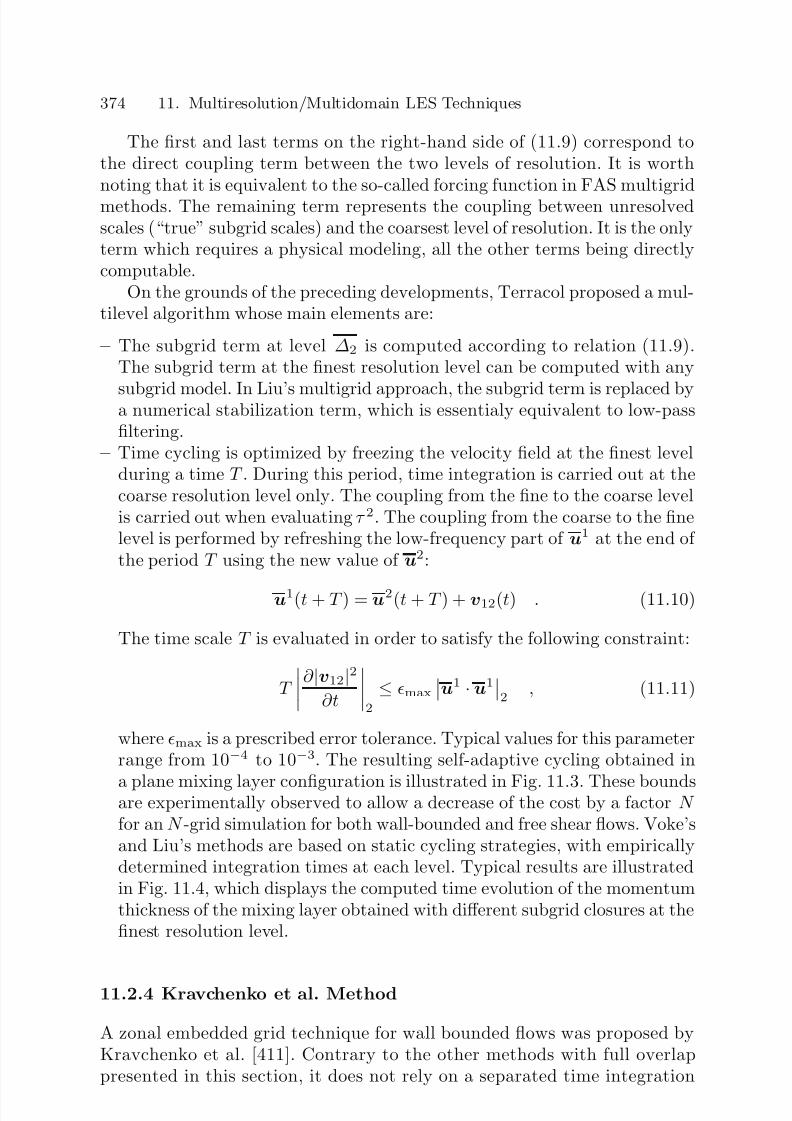
7/21/2019 Large Eddy Simulation for Incompressible Flows
http://slidepdf.com/reader/full/large-eddy-simulation-for-incompressible-flows 393/573
374 11. Multiresolution/Multidomain LES Techniques
The first and last terms on the right-hand side of (11.9) correspond tothe direct coupling term between the two levels of resolution. It is worthnoting that it is equivalent to the so-called forcing function in FAS multigridmethods. The remaining term represents the coupling between unresolvedscales (“true” subgrid scales) and the coarsest level of resolution. It is the onlyterm which requires a physical modeling, all the other terms being directlycomputable.
On the grounds of the preceding developments, Terracol proposed a mul-tilevel algorithm whose main elements are:
– The subgrid term at level ∆2 is computed according to relation (11.9).The subgrid term at the finest resolution level can be computed with any
subgrid model. In Liu’s multigrid approach, the subgrid term is replaced bya numerical stabilization term, which is essentialy equivalent to low-passfiltering.
– Time cycling is optimized by freezing the velocity field at the finest levelduring a time T . During this period, time integration is carried out at thecoarse resolution level only. The coupling from the fine to the coarse levelis carried out when evaluating τ 2. The coupling from the coarse to the finelevel is performed by refreshing the low-frequency part of u1 at the end of the period T using the new value of u2:
u1(t + T ) = u2(t + T ) + v12(t) . (11.10)
The time scale T is evaluated in order to satisfy the following constraint:
T
∂ |v12|2
∂t
2
≤ max
u1 · u1
2 , (11.11)
where max is a prescribed error tolerance. Typical values for this parameterrange from 10−4 to 10−3. The resulting self-adaptive cycling obtained in
a plane mixing layer configuration is illustrated in Fig. 11.3. These boundsare experimentally observed to allow a decrease of the cost by a factor N for an N -grid simulation for both wall-bounded and free shear flows. Voke’sand Liu’s methods are based on static cycling strategies, with empiricallydetermined integration times at each level. Typical results are illustratedin Fig. 11.4, which displays the computed time evolution of the momentumthickness of the mixing layer obtained with different subgrid closures at thefinest resolution level.
11.2.4 Kravchenko et al. Method
A zonal embedded grid technique for wall bounded flows was proposed byKravchenko et al. [411]. Contrary to the other methods with full overlappresented in this section, it does not rely on a separated time integration

7/21/2019 Large Eddy Simulation for Incompressible Flows
http://slidepdf.com/reader/full/large-eddy-simulation-for-incompressible-flows 394/573
11.2 Methods with Full Overlap 375
Fig. 11.3. Terracol’s self-adaptive time-cycling algorithm. Two-grid simulation of a plane mixing layer flow. Time history of the number of consecutive time-steps onthe coarse grid. Courtesy of M. Terracol, ONERA.
Fig. 11.4. Large-eddy simulation of a plane mixing layer using Terracol’s self-adaptive time-cycling algorithm with two resolution levels. Time evolution of themomentum thickness for different subgrid closures at the finest resolution level.Crosses correspond to classical large-eddy simulation on the coarse level. Courtesyof M. Terracol, ONERA.

7/21/2019 Large Eddy Simulation for Incompressible Flows
http://slidepdf.com/reader/full/large-eddy-simulation-for-incompressible-flows 395/573
376 11. Multiresolution/Multidomain LES Techniques
on each grid. The main element of the method is the use of a Galerkin-type numerical method with wide-stencil trial and weighting functions (fullynon-local, such as Fourier basis, or B-splines). The transfer of informationis intrinsically achieved thanks to the fact that the basis functions are notorthogonal.
In fact, this method can be interpreted as a particular case of the imple-mentation of Galerkin methods on unstructured grids.
11.3 Methods Without Full Overlap
We now describe the methods without full overlap, i.e. methods designed forthe case where the fine-resolution domain Ω 1 is not totally embedded into thecoarse-resolution domain Ω 2: Ω 1∩ Ω 2 = Ω 1. The partial overlap precludes theuse of multigrid-type algorithms like those presented in the previous section,and time integration must be carried synchronously in each domain. The datatransfer is done at each time step (or substep for multistep schemes) in orderto provide refreshed boundary conditions to the subdomains.
Quemere et al. [612] carried out an extensive analysis of the interfacingproblem between subdomains with different resolutions within the large-eddysimulation framework. The main results of their analysis are the following:
– From fine to coarse resolution subdomain: boundary conditions are ob-tained by filtering the data (point values or fluxes):
u2Γ
= G21 u1
Γ
, and/or G2 NS (u)|Γ = G21 G1 NS (u)|Γ ,
(11.12)with
Γ = ∂Ω 1 ∩ (Ω 1 ∩ Ω 2) . (11.13)
– From coarse to fine resolution subdomain: the definition of boundary con-
ditions for u1 requires two successive steps:1. Interpolation of u2 at the fine resolution level ∆1. This step is easy to
implement, and does not induce specific theoretical problems.2. Reconstruction of the complementary field v12. If Γ corresponds to an
exit boundary for the subdomain Ω 1, numerical experiments show thatthe enrichment step is not mandatory and v12 = 0 can be used. On thecontrary, if Γ is an inflow boundary condition for Ω 1, the reconstructionof v12 is necessary, and the enrichment step is theoretically equivalentto the definition of turbulent inflow conditions (see Sect. 10.3). All the
methods proposed for generating inflow turbulence can be used to pre-dict v12. A simple extrapolation procedure from the interior of Ω 1 canalso be used, if the elementary convection length U c∆t (with U c thecharacteristic advection velocity across Γ and ∆t the time step) is muchsmaller than the local correlation length scale of turbulent fluctuations.
7/21/2019 Large Eddy Simulation for Incompressible Flows
http://slidepdf.com/reader/full/large-eddy-simulation-for-incompressible-flows 396/573
11.4 Coupling Large-Eddy Simulation with Adaptive Mesh Refinement 377
Quemere et al. emphasized the fact that a weighted extrapolation canbe used to account for the spatial variation of the mean Reynolds stressprofiles.
3. Rescaling of the subgrid models. The coupling can also be completedby enforcing some compatibility conditions on the subgrid terms at theinterface. Inertial range arguments make it possible to derive propor-tionality factors. The following technique for rescaling subgrid viscositymodels was proposed in [612]. Starting with the classical relations
ν 1sgs ∝ ∆1
u
1 · u1 , ν 2sgs ∝ ∆2
u
2 · u2 , (11.14)
and assuming the orthogonality property
u2 · u
2 = (u1 + v12) · (u
1 + v12) ≈ u1 · u
1 + v12 · v12 , (11.15)
we obtain the following relation
ν 2sgs ∝
∆2
∆1
∆1
u
1 · u1 + v12 · v12 . (11.16)
From this last relation, we deduce a scaling law between the two viscosi-ties ν 2sgs
ν 1sgs
2
∝∆2
∆1
21 +
v12 · v12
u1 · u
1
, (11.17)
which can be used at the interface.
11.4 Coupling Large-Eddy Simulation with AdaptiveMesh Refinement
11.4.1 Statement of the Problem
The theoretical advantage of coupling with Adaptive Mesh Refinement(AMR) is twofold:
– Decrease in the mesh size ∆x results in a reduction of the discretizationerror, yielding an improved numerical accuracy.
– If the cutoff length ∆ is tied to ∆x, mesh refinement will also inducea decrease in ∆ and make the subgrid model less influential on the results(since a larger part of the exact solution is directly captured).
The philosophy of the AMR approach is that the grid refinement must beperformed automatically during the computation, leading to the definition of several open problems:

7/21/2019 Large Eddy Simulation for Incompressible Flows
http://slidepdf.com/reader/full/large-eddy-simulation-for-incompressible-flows 397/573
378 11. Multiresolution/Multidomain LES Techniques
– Finding an error estimate (the global error or each error source individu-ally) and defining a criterion (usually a threshold value) that will triggerthe refinement.
– Finding a bound for the algorithm: since projection error, discretizationerror and modeling error are present, an accurate error sensor should de-tect all of them, and a consistent unbounded AMR algorithm will convergetoward a Direct Numerical Simulation, leading to very high computationalcost. The method must then be bounded in the sense that the final solu-tion should correspond to a large-eddy simulation with potentially largeprojection error. This bound can be imposed in several ways: by fixinga maximum number of degrees of freedom, by giving a minimum mesh sizeor playing on the threshold level in the evaluation of the error.
11.4.2 Error Estimation
The criterion used to refine the grid is based on the definition of an errorestimate. Therefore, it relies on an a priori choice dealing with the quantitieswhose accuracy is the most important for the considered application. This isan arbitrary, user-dependent decision.
Since it should account for both the numerical and modeling errors, theerror estimate is closely tied to the numerical method and the subgrid modelused in the simulation. The optimal choice is therefore case dependent, andreveals a certain degree of empiricism.
The most striking achievements have been obtained by Hoffman [314,310, 312, 313] using an a posteriori error estimate within a finite elementframework. Less developed methods [149, 518, 268] will not be describedhere. The definition of an error estimate brings in many questions dealingwith mathematical analysis that will not be mentioned here. The interestedreader can refer to the original publications and the references given thereinfor more details. The presentation given below will be restricted to the main
features of the method.The purpose is to improve the accuracy of the simulation by error control
of the quantity
err(uΠ − ud) =
Q
(uΠ − ud) · ψdtdx , (11.18)
where ψ is a vectorial test function and the integration domain Q is definedas Q = Ω × I , where Ω is the volume of the computational domain and I
a time interval. The two velocity fields uΠ and ud are related to the idealsolution in which only the projection error is present and the computed so-lution including modeling and discretization errors, respectively. The aim of an AMR procedure based on (11.18) is therefore to eliminate modeling anddiscretization errors. This definition of the error is the most general one, andallows the definition of optimal control methods.
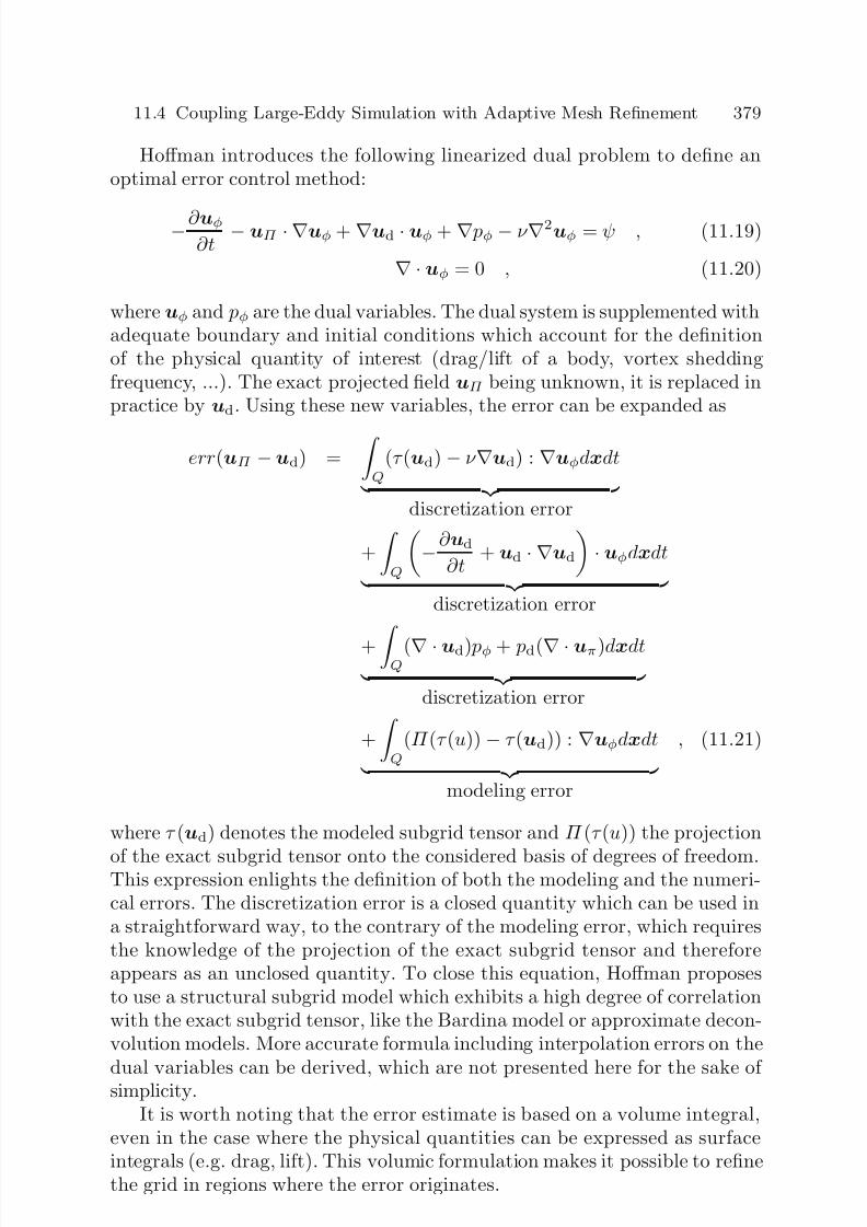
7/21/2019 Large Eddy Simulation for Incompressible Flows
http://slidepdf.com/reader/full/large-eddy-simulation-for-incompressible-flows 398/573
11.4 Coupling Large-Eddy Simulation with Adaptive Mesh Refinement 379
Hoffman introduces the following linearized dual problem to define anoptimal error control method:
−∂ uφ∂t
− uΠ · ∇uφ + ∇ud · uφ + ∇ pφ − ν ∇2uφ = ψ , (11.19)
∇ · uφ = 0 , (11.20)
where uφ and pφ are the dual variables. The dual system is supplemented withadequate boundary and initial conditions which account for the definitionof the physical quantity of interest (drag/lift of a body, vortex sheddingfrequency, ...). The exact projected field uΠ being unknown, it is replaced inpractice by ud. Using these new variables, the error can be expanded as
err(uΠ − ud) = Q
(τ (ud) − ν ∇ud) : ∇uφdxdt discretization error
+
Q
−∂ ud
∂t + ud · ∇ud
· uφdxdt
discretization error
+ Q
(∇ · ud) pφ + pd(∇ · uπ)dxdt discretization error
+
Q
(Π (τ (u)) − τ (ud)) : ∇uφdxdt modeling error
, (11.21)
where τ (ud) denotes the modeled subgrid tensor and Π (τ (u)) the projection
of the exact subgrid tensor onto the considered basis of degrees of freedom.This expression enlights the definition of both the modeling and the numeri-cal errors. The discretization error is a closed quantity which can be used ina straightforward way, to the contrary of the modeling error, which requiresthe knowledge of the projection of the exact subgrid tensor and thereforeappears as an unclosed quantity. To close this equation, Hoffman proposesto use a structural subgrid model which exhibits a high degree of correlationwith the exact subgrid tensor, like the Bardina model or approximate decon-volution models. More accurate formula including interpolation errors on the
dual variables can be derived, which are not presented here for the sake of simplicity.It is worth noting that the error estimate is based on a volume integral,
even in the case where the physical quantities can be expressed as surfaceintegrals (e.g. drag, lift). This volumic formulation makes it possible to refinethe grid in regions where the error originates.

7/21/2019 Large Eddy Simulation for Incompressible Flows
http://slidepdf.com/reader/full/large-eddy-simulation-for-incompressible-flows 399/573
380 11. Multiresolution/Multidomain LES Techniques
Fig. 11.5. LES-AMR simulation of the flow around a surface-mounted cube. Viewof the instantaneous flow Top: (x–y) plane: Bottom: (x–z) plane. Courtesy of J. Hoff-
man, Courant Institute.
Fig. 11.6. LES-AMR simulation of the flow around a surface-mounted cube. Viewof the grid after 9 refinement steps. Courtesy of J. Hoffman, Courant Institute .
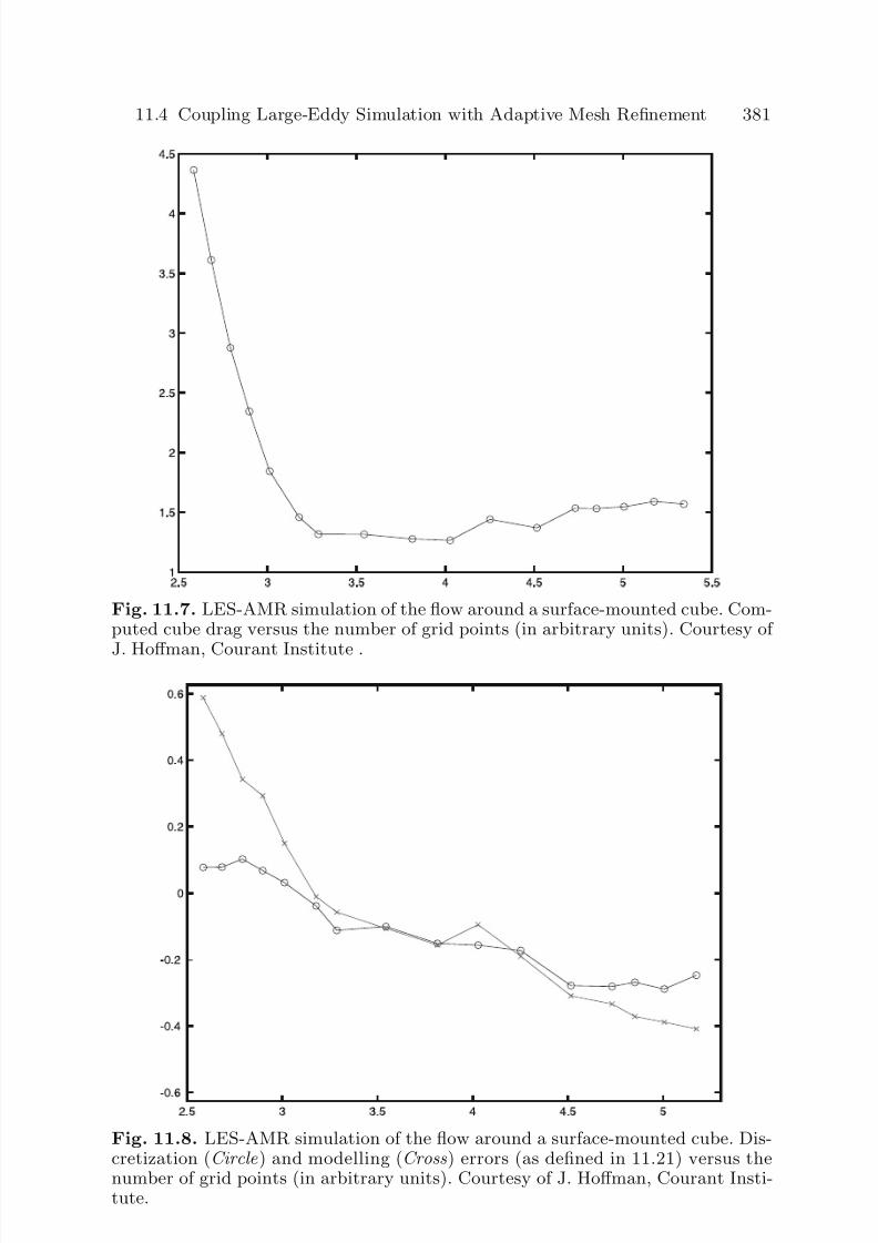
7/21/2019 Large Eddy Simulation for Incompressible Flows
http://slidepdf.com/reader/full/large-eddy-simulation-for-incompressible-flows 400/573
11.4 Coupling Large-Eddy Simulation with Adaptive Mesh Refinement 381
Fig. 11.7. LES-AMR simulation of the flow around a surface-mounted cube. Com-puted cube drag versus the number of grid points (in arbitrary units). Courtesy of
J. Hoffman, Courant Institute .
Fig. 11.8. LES-AMR simulation of the flow around a surface-mounted cube. Dis-cretization (Circle ) and modelling (Cross ) errors (as defined in 11.21) versus thenumber of grid points (in arbitrary units). Courtesy of J. Hoffman, Courant Insti-tute.

7/21/2019 Large Eddy Simulation for Incompressible Flows
http://slidepdf.com/reader/full/large-eddy-simulation-for-incompressible-flows 401/573
382 11. Multiresolution/Multidomain LES Techniques
The resulting algorithm is
1. Compute the solution (ud, pd) solving the large-eddy simulation govern-
ing equation over a time interval I .2. Solve the dual problem (11.19) – (11.20) to obtain (uφ, pφ) over I and
compute the discretization and modeling error according to (11.21).3. Refine the grid in zones where one or both error sources are higher than
a fixed threshold, taking into account possible bounds.4. Loop until the targeted level of accuracy is reached, i.e. until err(uΠ −ud)
is lower than a required value.
Good results were obtained dealing with the prediction of aerodynamicforces on bluff bodies, using a finite-element method on unstructured meshes.
Typical results obtained dealing with the prediction of the drag of a surface-mounted cube are displayed in Figs. 11.5 – 11.8.

7/21/2019 Large Eddy Simulation for Incompressible Flows
http://slidepdf.com/reader/full/large-eddy-simulation-for-incompressible-flows 402/573
12. Hybrid RANS/LES Approaches
12.1 Motivations and Presentation
This chapter is devoted to the presentation of hybrid RANS/LES methods.The main motivation for hybridizing the two methods is to decrease the costof the traditional large-eddy simulation method, which is large because of:
– the requirement to directly capture all the scales of motion responsible forturbulence production;
– the observed inability of most subgrid models to correctly account foranisotropy and disequilibrium.
These two weaknesses lead to the use of very-fine-resolution meshes, which
can be a real problem if the characteristic lengthscale of turbulence-pro-duction events is a decreasing function of the Reynolds number. A famousproblematic example is the inner region of boundary layers, whose intrinsicscale is the wall unit (see Sect. 10.2).
In order to alleviate this problem, a possible solution is to blend large-eddysimulation with another technique which must be able to provide relevantlower-frequency solutions at a much lower cost. A natural proposition is touse the RANS approach, which relies on a statistical average of the exactsolution and leads to a very large reduction of the number of degrees of
freedom in comparison with large-eddy simulation.The presently existing techniques can be classified as follows:
– Zonal decomposition (Sect. 12.2): the global computational domain isdivided into subdomains, some of them being treated with the RANSmethod, the other ones being computed using large-eddy simulation. Thegain comes from the fact that the grid resolution can be coarser in theRANS subdomains. Further cost reduction can be obtained when one ortwo spatial directions can be suppressed in the RANS subdomains thanksto statistical homogeneity of the flow in these directions.
– Nonlinear Disturbance Equations (Sect. 12.3): the idea here is to computethe mean flowfield or the low-frequency part of the solution using a RANSor unsteady RANS simulation, and to reconstruct the missing part of thefluctuating field using a large-eddy-type simulation. This approach can beinterpreted as a zonal multidomain approach in the frequency domain.
7/21/2019 Large Eddy Simulation for Incompressible Flows
http://slidepdf.com/reader/full/large-eddy-simulation-for-incompressible-flows 403/573
384 12. Hybrid RANS/LES Approaches
– Universal modeling (Sect. 12.4): the subgrid model is replaced by a newmodel, which appears as a generalized turbulence model defined as a com-bination of a RANS model and a typical subgrid model. The hope here isto obtain robust subgrid models, which are able to deal with very coarsegrids similar to those used in unsteady RANS computation. The mergingwith a RANS model is expected to introduce more physics into the subgridmodel, rendering it efficient if the cutoff is located in the low-frequency partof the spectrum, outside or at the very beginning of the inertial range.
12.2 Zonal Decomposition
12.2.1 Statement of the Problem
The zonal decomposition approach can be recast as a generalized multido-main/multiresolution problem. The main difference with the multidomainmethods presented in Chap. 11 is that the coupling is now performed be-tween subdomains where the scale separation is performed using operators of a different nature: filtering in large-eddy simulation and statistical averagingin RANS.
Equations presented in Sect. 11.1 can be reused in the present framework,keeping in mind that now G2 is related to statistical averaging:
φ2 ≡ G2(φ) =
1
N
i=1,N
φi = φ , (12.1)
where N is the number of samples chosen to compute the statistical average,while G1 is still defined as a convolution filter.
All the theoretical analyses presented in Sect. 11.1 can be directly ex-tended to the RANS/LES coupling method. The main practical difference isthat now the problem of the reconstruction of the complementary field v12 isstrictly equivalent to that of the definition of turbulent inflow conditions forlarge-eddy simulation described in Sect. 10.3. The mean flow is now predictedusing the RANS computation.
Another pratical difference is the definition of the restriction operator G21,
which is defined so that:
G21(G1 u) = G2(u) , (12.2)
or, equivalently, and using the usual notation:
G21(u1) = u . (12.3)
From a purely theoretical point of view, we see that G21 must be defined
as the sequential application of a deconvolution operator and statistical av-eraging. It can be simplified as a simple statistical average when the meanvelocity profiles of the exact and filtered solutions are equal.1
1 This condition is satisfied if the filter is applied in homogeneous directions only.

7/21/2019 Large Eddy Simulation for Incompressible Flows
http://slidepdf.com/reader/full/large-eddy-simulation-for-incompressible-flows 404/573
12.2 Zonal Decomposition 385
Two main approaches are identified:
– Sharp transition (Sect. 12.2.2): the reconstruction of the complementary
field is carried out explicitly at the interface between RANS and LES sub-domains, yielding a sharp transition over one grid mesh from one solutionto the other.
– Smooth transition (Sect. 12.2.3): the reconstruction of v12 is not performedat the interface, and the high-frequency part of the fluctuating field mustbe regenerated by instabilities of the mean flow and the forward energycascade. This approach leads to the existence of a transition region nearthe interface, whose width is case-dependent.
12.2.2 Sharp TransitionA method based on the sharp transition approach was proposed by Quemereet al. [610], and is an extension of the multidomain method proposed by thesame authors (see Sect. 11.3). It relies on a strict analogy between the recon-struction of the complementary field v12 and the definition of the turbulentinflow condition.
The G21 restriction operator is simply computed as a statistical average,
without incorporating a defiltering operator. Several techniques for recon-structing the fluctuations at the interface have been implemented (listed in
decreasing order of efficiency): use of a predictor simulation, Lund’s extrac-tion/rescaling technique, and random perturbation. Numerical experimentsshow that the smaller the transition region near the interface the more re-alistic the fluctuating field option becomes. When a predictor simulation isimplemented, it is reduced to one grid cell.
The method was applied with varying success to plane channel flow andflow around a blunt trailing edge. The RANS model was the Jones–Launderk–ε model. The boundary conditions for the turbulent quantities at the in-terface were derived from a simple extrapolation procedure. Typical results
for a plane channel flow configuration are presented in Figs. 12.1 and 12.2.A simplified version of Quemere’s approach was implemented by Geor-
giadis et al. [241], who operated the switch from RANS to LES while ne-glecting the reconstruction of the complementary field. The purpose was thesimulation of a mixing layer flow, in which the primary instabilities havea very large growth rate, resulting in a small influence of the exact definitionof the complementary field.
Applications of this approach to the definition of sophisticated two-layerwall models for large-eddy simulation have also been proposed by Davidson
et al. [167] and Diurno et al. [180]. In both cases, the complementary fieldis not reconstructed. The resolved field is assumed to be continuous at theinterface in Davidson’s method, which is based on a k−ω RANS model, whilethe coupling is achieved by transmiting wall stresses at the interface in Di-urno’s simulations relying on the Spalart–Allmaras model. Additional bound-ary conditions must be provided for turbulent quantities at the RANS/LES
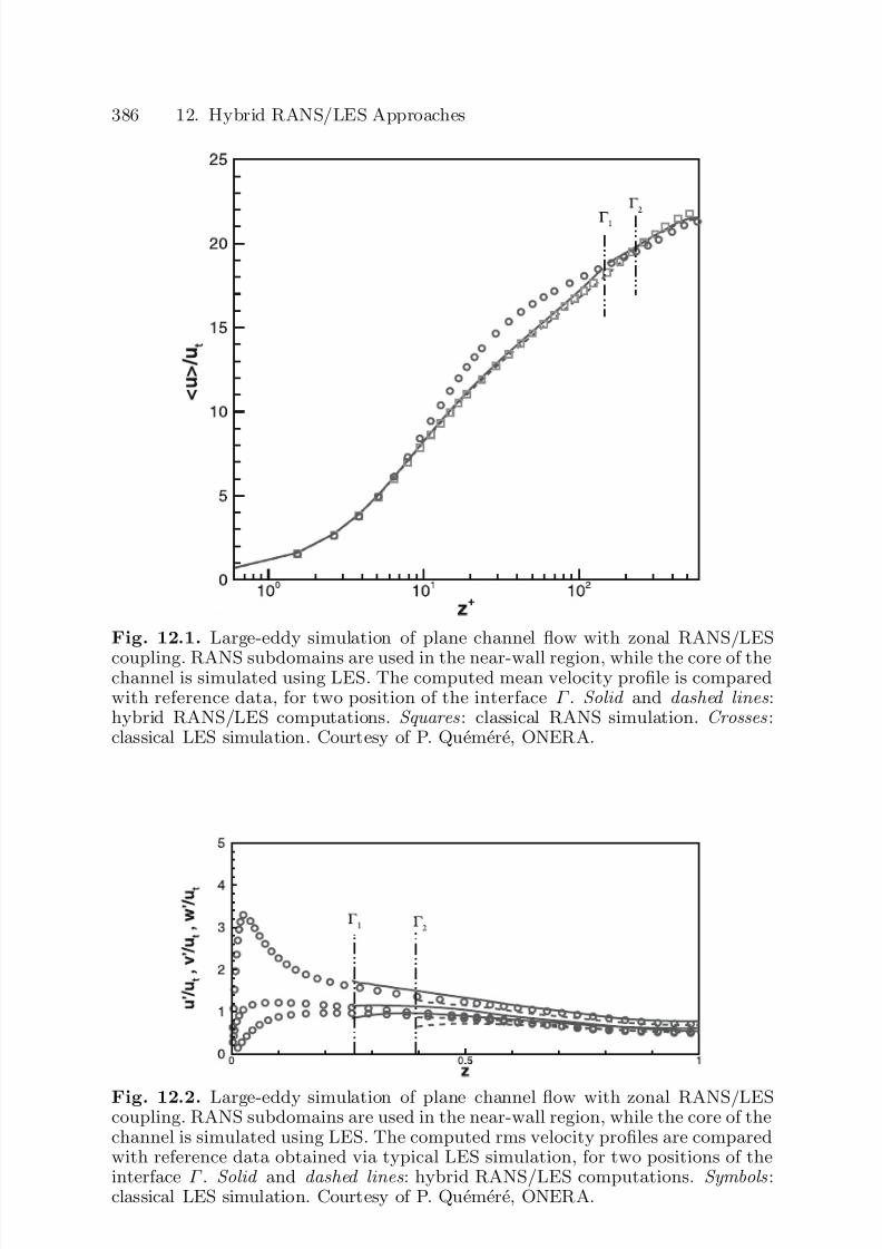
7/21/2019 Large Eddy Simulation for Incompressible Flows
http://slidepdf.com/reader/full/large-eddy-simulation-for-incompressible-flows 405/573
386 12. Hybrid RANS/LES Approaches
Fig. 12.1. Large-eddy simulation of plane channel flow with zonal RANS/LES
coupling. RANS subdomains are used in the near-wall region, while the core of thechannel is simulated using LES. The computed mean velocity profile is comparedwith reference data, for two position of the interface Γ . Solid and dashed lines :hybrid RANS/LES computations. Squares : classical RANS simulation. Crosses :classical LES simulation. Courtesy of P. Quemere, ONERA.
Fig. 12.2. Large-eddy simulation of plane channel flow with zonal RANS/LEScoupling. RANS subdomains are used in the near-wall region, while the core of thechannel is simulated using LES. The computed rms velocity profiles are comparedwith reference data obtained via typical LES simulation, for two positions of theinterface Γ . Solid and dashed lines : hybrid RANS/LES computations. Symbols :classical LES simulation. Courtesy of P. Quemere, ONERA.
7/21/2019 Large Eddy Simulation for Incompressible Flows
http://slidepdf.com/reader/full/large-eddy-simulation-for-incompressible-flows 406/573
12.2 Zonal Decomposition 387
interface. Davidson assumed no coupling at the interface for variables relatedto models and imposed arbitrary conditions, while explicit coupling is en-forced in Diurno’s method. The latter assumes that the total stress is equalon both sides of the interface.
12.2.3 Smooth Transition
Hybrid RANS/LES strategies presenting a smooth transition have all beenderived to alleviate the classical grid resolution requirements of classicallarge-eddy simulation in the near-wall region. Consequently, they can beinterpreted as hybrid wall-models for large-eddy simulation. Combinationsbetween the two basic techniques are derived in two different ways:
– By performing an explicit blending of the two basic models. Bagget [31]classified the existing approaches in two groups. The first one correspondsto the linear combination of the predicted turbulent/subgrid stresses:
τ ij − 1
3τ kkδ ij = −ν sgs
S ij − (1 − β (z))S ij
− β (z)ν ransS ij , (12.4)
where ν sgs and ν rans are the subgrid and turbulent viscosities, respectively.The arbitrary weight β (z) is expressed as a function of the distance to the
wall, and should be prescribed. This form of hybrid RANS/LES model is anextension of the splitting technique proposed by Schumann (see Sect. 6.3.3,p. 200) to account for anisotropy in the near-wall region. Methods belong-ing to the second group are based on the blending of the modeled viscosities:
τ ij − 1
3τ kkδ ij = − [(1 − β (z))ν sgs + β (z)ν rans] S ij . (12.5)
In both cases β = 0 corresponds to classical large-eddy simulations andβ = 1 to classical RANS simulations.
– Replacing the characteristic scales which explicitly appear in the RANSmodel equations by new scales corresponding to the LES filter. The impor-tant point is that the turbulent viscosity or the turbulent stresses are notdirectly rescaled, and consequently these quantities exhibit a continuousbehaviour, yielding smooth transition. The most famous example belong-ing to this category is the Detached Eddy Simulation proposed by Spalartet al. [680, 569]. This model is based on a modification of the Spalart–Allmaras RANS model, in which the distance to the wall d is replacedby d:
d = min(d, C des∆) , (12.6)
in the destruction term of the transport equation. The constant C des iscalibrated in order to recover a Smagorinsky-like behaviour in isotropicturbulence at equilibrium, yielding C des = 0.65. The Detached Eddy Sim-ulation approach has been extented by Strelets [16] to a large family of
7/21/2019 Large Eddy Simulation for Incompressible Flows
http://slidepdf.com/reader/full/large-eddy-simulation-for-incompressible-flows 407/573
388 12. Hybrid RANS/LES Approaches
RANS two-equation models. For a k–ω model, the characteristic lengthlk−ω ∝
√ k/ω is replaced in the dissipative term of the k-transport equa-
tion byl = min(lk−ω, C des∆), C des = 0.78 . (12.7)
A similar approach was developed by Tucker and Davidson [720] which re-lies on two-equation k–l models. In the RANS domain, a usual k–l modelis used, while the Yoshizawa k–l subgrid model is used in the LES subdo-main. The equations of these two models are formally equivalent, but withdifferent values of the constants appearing in them. The switch is achievedby changing the length scale in the transport equations: the usual RANSlength scale is used in the RANS subdomain, while the subgrid lengthscale
∆ is considered in the LES subdomain. This switch results in a discon-tinuous value of the length scale at the interface. Tucker and Davidsonobtain a regular distribution at the interface by applying a 3-point testfilter across the interface to the lengthscale.Another smooth transition method was proposed by Hamba [284]. In thismethod, the RANS and LES subdomains are overlapping, and the lengthscale in the subgrid model is assumed to vary linearly from the RANSlength scale to the usual subgrid length scale tied to the computationalmesh. Hamba applied this technique to a channel flow, hybridizing a k–ε
model and a Smagorinsky model. This method yields some error in themean velocity profile, and was further improved in [285]. In the improvedmethod, the dissipation ε is also linearly interpolated between the RANSvalue and the one predicted using the subgrid model. But the most impor-tant improvement factor is that the convective fluxes on each side at theinterface are estimated using an ad hoc interpolated velocity field whichis more compatible with the discrete mass preservation constraint. Thisblending of the two solutions at the interface can also be interpreted asa surrogate for the complementary field v12. The improved method is ob-served to yield much satisfactory results on a plane channel configura-tion.
12.2.4 Zonal RANS/LES Approach as Wall Model
Both sharp- and smooth-transition hybrid methods have been used to derivenew robust wall models for large-eddy simulation. Results are generally disap-pointing for methods which neglect the reconstruction of the complementaryfield at the interface. An artificial turbulent boundary layer develops, whichis composed of overly large streamwise streaks and vortices. This turbulentprocess is observed to be self-sustaining. This can be explained by theoreticaland numerical results dealing with the existence of a near-wall autonomouscycle [353, 354, 355, 750], which is created by the mean shear.
For sharp-transition methods, the problem is identical to that of wallmodels for large-eddy simulation, and it seems that zonal modeling cannot
7/21/2019 Large Eddy Simulation for Incompressible Flows
http://slidepdf.com/reader/full/large-eddy-simulation-for-incompressible-flows 408/573
12.2 Zonal Decomposition 389
perform better than the suboptimal-control-theory-based wall stress models(see Sect. 10.2).
For smooth-transition methods, the interface is replaced by a transition re-gion. An explanation [31] for the existence of a spurious near-wall cycle is thatthe no-slip boundary condition produces a near-wall viscous region in whichthe mean pressure gradient is balanced only by the mean viscous stress. Theflow is fully turbulent outside the transition region, so that the mean shearscales as 1/z, z being the wall-normal coordinate. In the transition region, themean shear has to be reduced by wall-normal streamwise momentum trans-port, i.e. mean Reynolds stress, to couple the core flow to the wall. If the sub-grid model does not carry a large enough amount of Reynolds stress, the re-solved motion will adjust in order to enforce the necessary balance. Some au-
thors tried to cure this problem by artificially enhancing the dissipation in thetransition region, but this method did not prove to be efficient and general.
For high-Reynolds-number boundary layers, the use of too coarse a gridalso yields significant errors in the mean velocity profiles [569]. This demon-strates that, even if the RANS region is able to provide the large-eddy simu-lation with correct boundary conditions, the grid resolution in the LES regionmust be the same as for classical wall-resolving large-eddy simulations.
Another point is that Quemere’s results seem to indicate that accountingfor the complementary field v12 at the interface improves the results and can
prevent the appearance of the spurious cycle.2
Applications to massively separated flows have also been perfomed [180,167, 146, 680, 695] which demonstrate that these hybrid approaches can yieldmuch more satisfactory results than for attached flows. The main reason isthat massively separated flows are mostly governed by inviscid, large-scaleinstabilities of the mean flow, which occur in the LES region. The quality of the results is then equivalent to that of a typical large-eddy simulation, butwith an effective cost reduction. Strelets [695] remarked that the numericalscheme must be adjusted to the selected approach in each region to obtain
reliable results: a low-order accurate dissipative method can be used in theRANS region, but not in the LES region. As a consequence, the zonal ap-proach for physical modeling can also imply the definition of a zonal approachfor the numerical method.
The concept of hybridizing RANS and large-eddy simulation in the near-wall region is fully general and does not depends, from a purely formal stand-point, on the modeling approaches used in both parts. The RANS simulationis almost always carried out using models relying on zero to three additionalequations, while subgrid models involving zero to two equations are very often
met. A noticeable exception is provided by Tucker [719], who couples a one-equation RANS model with a MILES approach in the large-eddy simulationdomain.
2 This is consistent with the finding that the use of a non-zero transpiration ve-locity for wall stress models yields improved results.
7/21/2019 Large Eddy Simulation for Incompressible Flows
http://slidepdf.com/reader/full/large-eddy-simulation-for-incompressible-flows 409/573
390 12. Hybrid RANS/LES Approaches
12.3 Nonlinear Disturbance Equations
Another hybrid RANS/LES method was proposed by Morris et al. [545,140, 288, 547], which is referred to as the Nonlinear Disturbance Equations(NLDE) method. The underlying idea is to split the field into a low-frequencyor steady part on the one hand, and a high-frequency fluctuating part. Theformer can be computed using steady or unsteady RANS simulations, or the-oretical laws, while the latter is computed via large-eddy simulation. Theresulting set of governing equations appears as a generalized form of theNavier–Stokes equations in perturbation form:
∂ u2
∂t + NS (u
2
) = τ 2
, (12.8)
∂ v12
∂t + NS (u1) − NS (u2) = τ 1 − τ 2 . (12.9)
An interesting difference with other methods presented above is that theequation for the detail v12 is solved, rather than the equation for the filteredfield u1. If the carrying field u2 is steady, the time derivative in (12.8) cancelsout, leading to
∂ v12
∂t =
∂ u1
∂t . (12.10)
If it is laminar, then τ 2 = 0.Using the bilinear form (3.27), the nonlinear convective term appearing
in (12.9) can be recast as
B(u1, u1) − B(u2, u2) = B(u2, v12) + B(v12, u2) I
+ B(v12, v12) II
. (12.11)
Terms I and I I are related to the coupling between the two levels of reso-
lution and to the nonlinear interactions between the fluctuations, respectively.Another coupling is achieved through the source term in the right-hand sideof (12.9), which is defined as the difference between the subgrid force and theReynolds forcing term.
This approach can be interpreted as a generalized multilevel simula-tion (see Sects. 7.7.7 and 11.2), in which the coarsest level is defined usinga statistical-average operator and not a convolution filter.
This technique was first developed by Morris et al. to evaluate acousticsources from a steady jet computation, on the basis of a nonlinear invis-
cid model equation for the fluctuations. Their second main approximation isthat mean-flow source terms in the nonlinear disturbance equations can beneglected. More recently, these authors added a subgrid model to the distur-bance equations, in order to take into account the effect of unresolved modes,leading to a true hybrid RANS/LES approach. They also reintroduced a partof the mean flow source term into the nonlinear disturbances equation. The
7/21/2019 Large Eddy Simulation for Incompressible Flows
http://slidepdf.com/reader/full/large-eddy-simulation-for-incompressible-flows 410/573
12.4 Universal Modeling 391
NLDE approach was used by Hansen et al. [288] to simulate the unsteady,two-dimensional laminar flow around a circular cylinder, corresponding to thefirst coupling between NLDE and an unsteady mean flow. The first attemptto use it for wall-bounded flow is due to Chyczewski et al. [140], with fairlygood results due to the use of very coarse grids.
A fully general expression of the governing equations for nonlinear dis-turbance equations for compressible flows was derived by Labourasse andSagaut [416] who also proposed using this method to locally reconstruct theunsteady turbulent motion in subdomains embedded within the full flow con-figuration. This corresponds to a coupling between the nonlinear disturbanceequations approach and the multidomain method presented above. The ex-pected gain with respect to the classical large-eddy simulation approach is
twofold:
– Firstly, the mean field being prescribed, the errors commited on turbulentfluctuations will not pollute it, and we can expect this method to be morerobust than classical large-eddy simulation.
– Secondly, if the turbulence-producing events are localized in a small region,it will be possible to restrict the LES-type computation to a small subdo-main included in the global domain, while classical large-eddy simulationwould require us to consider the full domain.
Numerical experiments show that this method is more robust than theusual large-eddy simulation if the mean flow is correctly prescribed, i.e.coarser grids can be employed without loss of accuracy. Errors on the meanflow field u2 can be corrected using the hybrid approach on a fine grid: thefluctuating field will adjust such that (u2 + G2
1 v12) will be correct.
12.4 Universal Modeling
The last class of hybrid RANS/LES methods presented in this chapter is thatof the universal models. The underlying idea here is to design new modelswhich can asymptotically recover typical RANS or typical LES capabilities.The existing models are based on the rescaling of the RANS models thanksto inertial range arguments. They all aim at decreasing the resolved kineticenergy dissipation induced by the model for the unresolved scales. This de-crease in the induced dissipation leads to a weaker damping of high frequen-cies/high wavenumbers which can be sustained on the selected computationalgrid, yielding the recovery more irregular “LES-like” flowfields. Despite this
strategy is clear and does not suffer any flaw, it is worth noting that thedifferent methods used to achieve this reduction in the small scale damping3
are mostly empirical. The most common strategies found in the literature
3 The most common method is to reduce the amplitude of the turbulent viscosityof the RANS model.

7/21/2019 Large Eddy Simulation for Incompressible Flows
http://slidepdf.com/reader/full/large-eddy-simulation-for-incompressible-flows 411/573
392 12. Hybrid RANS/LES Approaches
deal with the modification of eddy-viscosity-type RANS models, and can begrouped in two classes:
1. The methods based on a rescaling of the eddy viscosity provided by theRANS model.
2. The methods based on the modification of some terms in the transportequations of the original RANS model, so as to reduce the amplitude of the eddy viscosity. In the case of most RANS models which include anevolution equation for the turbulent kinetic energy, k, this is achieved byincreasing the destruction of k and/or modifying the second variable (if any).
A few hybrid models are presented below:
1. Germano’s mixed modeling (Sect. 12.4.1).2. Speziale’s general rescaling method for turbulent stresses (Sect. 12.4.2).3. Arunajatesan’s modified two-equation model (Sect 12.4.4).4. Bush–Mani limiters (Sect. 12.4.5).
12.4.1 Germano’s Hybrid Model
A general approach for the definition of hybrid RANS/LES models was pro-
posed by Germano [249]. This approach relies on two basic hypotheses:– The statistical value of a filtered quantity is equal to the statistical value
of the unfiltered quantity:
φ = φ . (12.12)
– The filtered solution is characterized by the associated mean production of subgrid kinetic energy:
τ les,ijS ij = C f τ rans,ijS ij , (12.13)
where τ les(u) and τ rans(u) are the subgrid and Reynolds stress tensor,respectively, and C f is a constant.
The first hypothesis makes it possible to decompose the modeled Reynoldsstress tensor as follows:
τ rans(u) = τ les(u) + τ rans(u) , (12.14)
while the second hypothesis leads to
τ les,ijS ij = C f
1 − C f τ rans,ij(u)S ij . (12.15)
This equation establishes a bridge between the modeled tensors at bothfiltered and statistically averaged levels. For subgrid viscosity models, we
7/21/2019 Large Eddy Simulation for Incompressible Flows
http://slidepdf.com/reader/full/large-eddy-simulation-for-incompressible-flows 412/573
12.4 Universal Modeling 393
obtain the following definition:
ν les =
C f
|S
|2(1 − C f )
τ rans,ij(u)
S ij
|S |S ijS ij . (12.16)
The parameter C f ∈ [0, 1] determines the respective weights of the fil-tered and the Reynolds-averaged parts. The RANS solution is recovered asC f −→ 1. The convergence of the method depends on the capability of theRANS model for τ rans,ij , once applied to the filtered field u, to alleviate thesingular behavior of (12.16).
12.4.2 Speziale’s Rescaling Method and Related Approaches
Models belonging to this category can be expressed as
τ ij = F Rτ ransij , (12.17)
where F R is the rescaling function to be defined, and τ ransij the modeled
turbulent stress tensor predicted using any RANS model.Speziale [685, 684] proposed a general rescaling function
F R =
1 − exp(−β∆/ηK )
n, (12.18)
where β is a constant, n an arbitrary power, and ηK the Kolmogorov lengthscale computed from the variables of the RANS model. The direct numer-ical simulation regime is recovered as the limit of a very fine resolution,∆/ηK −→ 0. As the resolution becomes very coarse, ∆/ηK −→ ∞, theRANS model is recovered. As noted by Magnient [477], a consistency prob-lem of the Speziale’s transition function is that large-eddy simulation is notrecovered as a limit for very high Reynolds number.4 In practice, Spezialerecommended applying this scaling law to complex RANS models able todeal with anisotropy and disequilibrium, such as Reynolds Stress Models or
Explicit Algebraic Reynolds Stress Models. Proposed values in [685, 684] areβ = 0.001 and n = 1, but the model is expected to be very sensitive to theseparameters.
Fasel [212] later used β = 0.004, ∆ = (∆1∆2∆3)1/3 and ηK = Re−3/4ε−1/4
together with an Explicit Algebraic Resynolds Stress Model to compute a flatplate boundary layer (ε being evaluated from the outputs of the RANSmodel). The same authors used a slightly modified version to compute a wall
jet flow. Parameters for this configuration are
F R = 1 − exp(− max(0, 5∆ − 10ηK )/N ηK ) , ∆ = 13 ∆2
1∆22∆2
3 ,
(12.19)
4 A well known example is isotropic turbulence in the limit of an infinite Reynoldsnumber.

7/21/2019 Large Eddy Simulation for Incompressible Flows
http://slidepdf.com/reader/full/large-eddy-simulation-for-incompressible-flows 413/573
394 12. Hybrid RANS/LES Approaches
where N is an adjustable parameter that governs the cutoff, which taken inthe range 1000–2000 in the wall-jet application.
A much simpler rescaling for computing subgrid viscosity was proposedby Peltier et al. [796, 584]. Using inertial range argument and numerical tests,these authors proposed computing the subgrid viscosity ν sgs from the RANSeddy viscosity ν rans as
ν sgs =
∆
l
2
ν rans , (12.20)
where l is the turbulent length computed using the RANS model outputs.Magnient [477] proposed a similar rescaling law for the RANS viscosity withthe power 4/3 instead of 2.
The rescaling approach was further developed by Batten and his co-workers [46, 47, 48, 49] as the Limited-Numerical-Scales method , who in-troduced the following rescaling factor:
F R = min[(LsgsU sgs), (LransU rans)]
(LransU rans) , (12.21)
where Lsgs, U sgs, Lrans, U rans are the characteristic subgrid length scale, sub-grid velocity scale, turbulent length scale and turbulent velocity scale, re-spectively. In the simple case where eddy viscosity type models are used in
both cases, the products LU are equal to the eddy viscosities. The origi-nal implementation by Batten for several flows rely on the nonlinear k–εmodel of Goldberg and the Smagorinsky model. It is important noticing thatthe subgrid closure is used here only to evaluate the rescaling factor F Rthrough (12.21). This method, coined as the Limited Numerical Scale ap-proach, was mainly used through a zonal implementation. To improve theresults, Batten strongly recommend to add explicit fluctuations at the inter-face, i.e. to synthetize explicitly the field v12.
12.4.3 Baurle’s Blending Strategy
A more complex method, which can be interpreted as an evolution of Bat-ten’s proposal using the same strategy as the one underlying Menter’s hybridRANS model, is presented by Baurle and his co-workers [50]. The underlyingidea is still to hybridize a classical RANS model with a standard subgrid scalemodel. A requirement is that both RANS and LES models include an equa-tion on the unresolved turbulent kinetic energy (TKE). The hybrid model istherefore defined by a linear combination of each model equation set:
Hybrid RANS/LES TKE equation =
F × [RANS TKE equation]
+(1 − F ) × [LES TKE equation] , (12.22)
7/21/2019 Large Eddy Simulation for Incompressible Flows
http://slidepdf.com/reader/full/large-eddy-simulation-for-incompressible-flows 414/573
12.4 Universal Modeling 395
andν hybrid = F ν rans + (1 − F )ν sgs . (12.23)
where F is a weighting function to be discussed below. As remarked byBaurle, an algebraic subgrid viscosity model or even an implicit model canalso be considered in this approach by constructing a production/destructionbalance equation for the subgrid kinetic energy that recovers the desired sub-grid viscosity. The key parameter in this approach is the weighting functionF . In the case F depends only on geometric factors such as the distance tosolid walls and on grid topology, the blending strategy results in a purelyzonal approach reminiscent to those described in Sect. 12.2. The blendingfunction proposed in Ref. [50] is more general and includes some information
tied to the level of resolution of the flow. It is defined as
F = max(tanh(ξ 4), F 1) , (12.24)
whith
ξ = max
Lrans
d , 500ν
C dLrans√ kransd2
, (12.25)
where Lrans, d and krans are the turbulent length scale computed from theRANS model outputs, the distance to the nearest wall and the turbulentkinetic energy provided by the RANS model, respectively. The constant C
dis taken equal to 0.01. The function F 1 is defined on the grounds of Batten’sblending function (12.21):
F 1 =
1 if ν sgs < ν rans
0 otherwise . (12.26)
The resulting weigthing function is such that the RANS treatment will beinvoked near solid surfaces, while the LES treatment will govern the simula-tion in separated and free shear regions. The introduction of the F 1 parameter
allows to maintain the RANS treatment when sudden grid refinements areencountered and that no resolved fluctuations are present.
A simplified version of the weighting function was developed in [772],which is expressed as
F = tanh
ν sgs
ν rans
2
. (12.27)
This approach is now illustrated considering the case of the two-equationsk − ζ model (ζ being the turbulent enstrophy) treated in [772]. The RANSequation for the turbulent kinetic energy k is:
∂ρk
∂t +
∂ρ ujk
∂xj=
∂
∂xj
µ
3 +
µrans
σk
∂k
∂xj
+ τ ij
∂ui∂xj
− 1
C k
µrans
ρ2
∂ρ
∂xi
∂p
∂xi− C 1
ρk
τ p− µζ , (12.28)
7/21/2019 Large Eddy Simulation for Incompressible Flows
http://slidepdf.com/reader/full/large-eddy-simulation-for-incompressible-flows 415/573
396 12. Hybrid RANS/LES Approaches
where
ν rans = µrans
ρ = C µ
k2
νζ , (12.29)
with C µ = 0.09, C k, C 1 and σk model-dependent parameters. The subgridviscosity being evaluated as
ν sgs = C s∆√
k, C s = 0.01 , (12.30)
the hybrid viscosity is defined according to (12.23) while the original turbu-lent kinetic energy equation (12.28) is transformed into
∂ρk
∂t
+ ∂ρ ujk
∂xj=
∂
∂xj µ
3
+ µhybrid
σk ∂k
∂xj+ τ ij∂ui
∂xj
−(1 − F )
1
C k
µhybrid
ρ2
∂ρ
∂xi
∂p
∂xi+ C 1
ρk
τ p+ µζ
−F C dρ
k3/2
∆, (12.31)
where C d = 0.01 is a constant. The RANS turbulent length scale appearingin the computation of the blending function is
Lrans = k
3/2
νζ . (12.32)
12.4.4 Arunajatesan’s Modified Two-Equation Model
A modified two-equation k–ε model was proposed by Arunajatesan et al. [20,21, 22] as a basis for hybrid RANS/LES simulations. The key idea is simi-lar to that of the Detached Eddy Simulation, i.e. some characteristic scalesappearing in the classical RANS model are replaced by new ones associatedwith the filtering operator. Two transport equations are solved along with theNavier–Stokes equations: one for the subgrid kinetic energy q sgs and one forthe total dissipation rate ε. Based on the values of these quantities and thefilter length ∆, a RANS and a subgrid viscosity referred to as ν rans and ν sgs,respectively, are computed. The subgrid viscosity is used in the equations formomentum and subgrid kinetic energy, while the RANS viscosity is used inthe equation for the turbulent dissipation rate.
The proposed transport equations for the subgrid kinetic energy and thedissipation rate are
∂q sgs
∂t + ∂
∂xiuiq sgs − (ν + ν sgs/σq) ∂q sgs
∂xi = P q − ε , (12.33)
∂ε
∂t +
∂
∂xi
uiε − (ν + ν rans/σε)
∂ε
∂xi
= P ε − Dε , (12.34)
7/21/2019 Large Eddy Simulation for Incompressible Flows
http://slidepdf.com/reader/full/large-eddy-simulation-for-incompressible-flows 416/573
12.4 Universal Modeling 397
where σk and σε are modeling constants equal to their usual RANS counter-parts. Production and dissipation terms appearing on the right-hand sidesof (12.33) and (12.34) are identical to those of the original RANS model andwill not be detailed here (see [424]).
Once these two quantities are known, it is assumed that the local turbulentenergy spectrum can be represented everywhere using the following hybridVon Karman/Pao form:
E (k) = C 1k−5/3∗
k
k∗
41 +
k
k∗
2−17/6
exp
−9
4k4/3
, (12.35)
where k = kηK is the normalized wave number, ηK the Kolmogorov lengthscale, k∗ the energy-containing wave number, E = E/(ν 5ε)1/4 the normalizedspectrum, and C 1 a constant to be determined.
The Kolmogorov scale is computed as ηK = (ν 3/ε)1/4. The constant C 1is chosen so that the integral of the dissipation range spectrum is equal tothe local turbulence dissipation rate.
The energy-containing wave number k∗ is computed in order to enforcethe following relation:
q sgs = ∞
π/∆ E (k)dk . (12.36)
Once the local turbulence spectrum is completely determined, the authorspropose computing the value of the subgrid viscosity for any cutoff wavenumber using the constant spectral subgrid viscosity model (5.19), yielding
ν sgs = 0.28
E (π/∆)
π∆, (12.37)
ν rans = 0.28 E (k∗)k∗
. (12.38)
12.4.5 Bush–Mani Limiters
Another possibility proposed by Bush and Mani [792] for deriving a hybridmodel is to generalize the basic idea underlying Spalart’s Detached EddySimulation by applying it to all the turbulent variables. Considering the two-equation RANS model of the general form k
−φ, the proposed solution is
summarized in Table 12.1. In order to account for both space- and time-filterings, the authors proposed redefining the filter length in the dissipationterm as ∆ = max(∆, |u|∆t,
√ k∆t) , (12.39)

7/21/2019 Large Eddy Simulation for Incompressible Flows
http://slidepdf.com/reader/full/large-eddy-simulation-for-incompressible-flows 417/573
398 12. Hybrid RANS/LES Approaches
Table 12.1. Bush–Mani limiters for hybrid RANS/LES models. C i are constants,
and
∆ is the cutoff length.
φ limiter
l min(l, C 1 ∆)
ε max(ε, C 2k3/2/ ∆)
ω max(ω, C 3k1/2/ ∆)
where ∆ is the usual cutoff length used in large-eddy simulation, and ∆t thetime step of the computation.
The same approach was followed by Allen and Mendonca [10], who testedextended versions of Spalart’s Detached Eddy Simulation based on severaltwo-equations models. The values of the constants appearing in Table 12.1given by these authors are C 2 = 0.73 and C 3 = 0.61. But numerical exper-iments reported by several authors indicate that the optimal value is case-dependent.
12.4.6 Magagnato’s Two-Equation Model
A modified two-equation model approach is proposed by Magnagato andGabi [476], which includes an explicit random backscatter term. The originalformulation of the model is based on either a non-linear k − ε or a non-lineark − τ RANS model, in which the characteristic length scale L is evaluated as
L = max
∆, |u|∆t
. (12.40)
Here, quantities computed solving the equations of the RANS model withthe modified length scale are assumed to be related to the unresolved turbu-
lent fluctuations. The dissipative part of the model is then written as
τ ij = −C µkτ S ij + 2
3kδ ij , (12.41)
for the k − τ model, and
τ ij = −C µk2
ε S ij +
2
3kδ ij , (12.42)
for the k −
ε model. In both cases, the value C µ = 0.09 is retained. Theauthors thus add a non-dissipative term to the expressions given above forthe subgrid tensor to account for the backscatter phenomenon. The genericform of the backscatter model is
τ ij = vivj − 2
3kδ ij (12.43)
7/21/2019 Large Eddy Simulation for Incompressible Flows
http://slidepdf.com/reader/full/large-eddy-simulation-for-incompressible-flows 418/573
12.5 Toward a Theoretical Status for Hybrid RANS/LES Approaches 399
where the random velocities vi are calculated at each time step usinga Langevin-type equation. Introducing ζ i an independent random vectorranging from
−1 to 1, the value of vi at the nth time step is defined as
vni = vn−1i
1 − ∆t
τ
+
∆t
τ
2 − ∆t
τ
2
3kζ ni , (12.44)
where the subgrid time scale τ is directly provided by the k − τ model andis evaluated as
τ = L√
k∞, (12.45)
for the k−
ε model, where the length scale L is given by relation (12.40) andk∞ is the sum of the resolved and the unresolved kinetic energy. The fullmodel formulation is obtained by adding the backscatter term to the selecteddissipative part.
12.5 Toward a Theoretical Status for HybridRANS/LES Approaches
Since they are based on the hybridization of the classical Large-Eddy Sim-ulation and Reynolds-Averaged Numerical Simulation methods, most of thehybrid approaches presented above escape the usual theoretical frameworkdeveloped to present them. As a matter of fact, the resulting flow field canneither be interpreted in terms of statistical average of the exact solution noras the result of a conventional filtering operation. Therefore, the questionarises of finding a relevant paradigm to analyze and understand these hybridapproaches.
A powerful framework to understand the properties of these methodsis the unresolved-scale-model induced effective filter paradigm developed byMuchinsky (see Sect. 8.1.1). This analysis is based on the observation that,during the computation, the only term which carries some information aboutthe unresolved scales is the turbulence/subgrid model5. Therefore, it is themodel for the unresolved scales which determines the amount of damping (thenumerical errors are assumed to be negligible here for the sake of clarity) of the resolved scales and governs the effective filtering of the exact solution.
This is illustrated writing the resolved discrete problem as
δud
δt
+ F d(ud, ud) = S d , (12.46)
where ud, δ/δt and F d(·, ·) are the discrete approximations of the exact termsu, ∂/∂t and F (·, ·) on the computational grid, respectively. Here, F (·, ·) is
5 In the case of the Implicit Large-Eddy Simulation approach, this information iscontained in the numerical errors.

7/21/2019 Large Eddy Simulation for Incompressible Flows
http://slidepdf.com/reader/full/large-eddy-simulation-for-incompressible-flows 419/573
400 12. Hybrid RANS/LES Approaches
related to the fluxes in the exact Navier–Stokes equations. The source termS d stands for the model for the unresolved scales.
The discrete equation for the resolved kinetic energy is
1
2
δu2d
δt + ud · F d(ud, ud) = ud · S d . (12.47)
The term in the right hand side of this new equation shows how themodel for unresolved scales governs the dissipation process. A decrease inthis dissipation will results in a larger amount of resolved kinetic energy, andtherefore to the existence of smaller scales (the limit being fixed by the gridresolution). All hybrid RANS/LES methods based on the modification or the
rescaling of a RANS model aim at decreasing this term.Following Muchinsky’s analysis, which relies on the idea that the RANSor LES computations can be seen as direct numerical simulations of a non-newtonian fluid, the observed effects of the modification of the original RANSmodels can be easily interpreted. The steady RANS solution corresponds toa steady laminar non-newtonian flow. Reduction in the dissipation results ina higher Reynolds number. Unsteady RANS solutions are therefore similarto direct numerical simulations of unsteady non-newtonian flow. The bifur-cations sometimes observed in unsteady RANS simulations when the totaldissipation is further reduced can be interpreted as analogous to bifurca-tions of a laminar newtonian flow at low-Reynolds number (transtition tothree-dimensional modes, growth of small scales, ...). The further dissipa-tion reduction achieved by the definition of hybrid models leads to higherReynolds numbers, and to the possiblity for smaller scales to be sustained.

7/21/2019 Large Eddy Simulation for Incompressible Flows
http://slidepdf.com/reader/full/large-eddy-simulation-for-incompressible-flows 420/573
13. Implementation
This chapter is devoted to the practical details of implementing the large-eddy simulation technique. The following are described:
– Cutoff length computation procedures for an arbitrary grid;– Discrete test filters used for computing the subgrid models or in a pre-
filtering technique;– Computing the Structure Function model on an arbitrary grid.
This part of the implementation of large-eddy simulation is more andmore recognized as one of the keys of the success of a simulation. Most of the theoretical developments rely on an abstract filter, which is characterizedby its cutoff frequency. But practical experience show that computational
results can be very sensitive to the effective properties (transfer function,cutoff length) of the fitering operators used during the simulation.
This is especially true of subgrid models relying on the use of a testfilter, such as dynamic models and scale-similarity models. Thus, the problemof the consistency of the filter with the subgrid model must be taken intoaccount [597, 563, 81, 641, 605].
13.1 Filter Identification. Computing the Cutoff Length
The theoretical developments of the previous chapters have identified severalfilters of different origins:
1. Analytical filter, represented by a convolution product. This is the filterused for expressing the filtered Navier–Stokes equations.
2. Filter associated with a given computational grid. No frequency higherthan the Nyquist frequency associated with this grid can be representedin the simulation.
3. Filter induced by the numerical scheme. The error committed by approxi-mating the partial derivative operators by discrete operators modifies thecomputed solution mainly the high-frequency modes.
4. Filter associated with the subgrid model, which acts like a control processon the computed solution.

7/21/2019 Large Eddy Simulation for Incompressible Flows
http://slidepdf.com/reader/full/large-eddy-simulation-for-incompressible-flows 421/573
402 13. Implementation
The computed solution is the result of these four filtering processes consti-tuting the simulation effective filter. When performing a computation, then,the question arises as to what the effective filter is, that governs the dynam-ics of the numerical solution, in order to determine the characteristic cutoff length. This length is needed for several reasons.
– In order to be able to determine the physically and numerically well-resolved scale beyond which we will be able to start using the results foranalysis.
– In order to be able to use the subgrid models like the subgrid viscositymodels that use this cutoff length explicitly.
While the filters mentioned above are definable theoretically, they are
almost never quantifiable in practice. This is particularly true of the filterassociated with the numerical schemes used. In face of this uncertainty, prac-titioners have one of two positions they can adopt:
1. Arrange it so that one of the four filters becomes predominant over theothers and is controllable. The effective filter is then known. This is donein practice by using a pre-filtering technique.Normally, this is done by ensuring the dominance of the analytical filter,which allows us strict control of the form of the filter and of its cut-
off length, so that we can get the most out of the theoretical analysesand thereby minimize the relative uncertainty concerning the nature of the computed solution. In the numerical solution, an analytical filter isthen applied here to each computed term. In order for this filter to bedominant, its cutoff length must be large compared with the other three.Theoretically, this analytical filter should be a convolution filter which, tokeep the computation cost within acceptable limits, can only be appliedfor simulations performed in the spectral space1. For the simulations per-formed in the physical space, discrete filters are used, based on weightedaverages with compact support. These operators enter into the categoryof explicit discrete filters, which are discussed in the following section.We may point out here that the methods based on implicit diffusionwith no physical subgrid model can be re-interpreted as a pre-filteringmethod, in which case it is the numerical filter that is dominant. We cansee the major problem of this approach looming here: the filter associatedwith a numerical method is often unknown and is highly dependent onthe simulation parameters (grid, boundary conditions, regularity of thesolution, and so forth). This approach is therefore an empirical one thatoffers little in the way of an a priori guarantee of the quality of the results.
It does, however, have the advantage of minimizing the computationcosts because we are then limited to solving the Navier–Stokes equationswithout implanting any subgrid model or explicit discrete filter.
1 The convolution product is then reduced to a simple product of two arrays.

7/21/2019 Large Eddy Simulation for Incompressible Flows
http://slidepdf.com/reader/full/large-eddy-simulation-for-incompressible-flows 422/573
13.1 Filter Identification. Computing the Cutoff Length 403
2. Considering that the effective filter is associated with the computationalgrid. This position, which can be qualified as minimalist on the theoreticallevel, is based on the intuitive idea that the frequency cutoff associatedwith a fixed computational grid is unavoidable and that this filter istherefore always present. The problem then consists in determining thecutoff length associated with the grid at each point, in order to be ableto use the subgrid models.In the case of a Cartesian grid, we take the filtering cell itself as Cartesian.The cutoff length ∆ is evaluated locally as follows:– For uniform grid, the characteristic filtering length in each direction is
taken equal to the mesh size in this same direction:
∆i = ∆xi . (13.1)
The cutoff length is then evaluated by means of one of the formulaspresented in Chap. 6.
– For a variable mesh size grid, the cutoff length in the ith direction of the grid point of index l is computed as:
∆i|l = (xi|l+1 − xi|l−1)/2 . (13.2)
The cutoff length is then computed locally according to the results of Chap. 6.
In the case of a curvilinear structured grid, two options are possibledepending on the way the partial derivative operators are constructed:– If the method is of the finite volume type in the sense of Vinokur [733],
i.e. if the control volumes are defined directly on the grid in the phys-ical space and their topologies are described by the volume of thecontrol cells, by the area and the unit normal vector to each of theirfacets, the filter cutoff length can be computed at each point either bytaking it equal to the cube root of the control volume to which the
point considered belongs, or by using what Bardina et al. propose (seeSect. 6.2.3).
– If the method is of the finite differences type in the Vinokur sense [733],i.e. if the partial derivative operators are computed on a uniform Carte-sian grid after a change of variables whose Jacobian is denoted J , thenthe cutoff length can be evaluated at the point of index (l ,m,n) eitherby Bardina’s method or by the relation:
∆l,m,n = (J l,m,n∆ξ∆η∆ζ )1/3 , (13.3)
where ∆ξ , ∆η and ∆ζ are the grid steps in the reference space.In the case of an unstructured grid, we use the same evaluations as fora structured curvilinear grid with a finite volume type method, in thesense given above.
7/21/2019 Large Eddy Simulation for Incompressible Flows
http://slidepdf.com/reader/full/large-eddy-simulation-for-incompressible-flows 423/573
404 13. Implementation
13.2 Explicit Discrete Filters
Several techniques and subgrid models described in the previous chapters usea test filter. For reference, these are the:
– Pre-filtering technique;– Soft deconvolution models and scale similarity models;– Mixed Scale Model;– Dynamic constant adjustment procedures;– Models incorporating a structural sensor;– Accentuation procedure.
The corresponding theoretical developments all assume that we are able
to apply an analytical filter in the simulation. This operation comes downto a product of two arrays in the spectral space, which is a simple operationof little cost, and all the analytical filters whose transfer function is knownexplicitly can be used. The problem is very different, though, when we con-sider the simulations performed in the physical space on bounded domains:applying a convolution filter becomes very costly and non-local filters cannotbe employed. In order to be able to use the models and techniques mentionedabove, we have to use discrete filters with compact support in the physicalspace. These are described in the rest of this section. These discrete filters
are defined as linear combinations of the values at points neighboring the onewhere the filtered quantity is computed [632, 728, 563, 461].
The weighting coefficients of these linear combinations can be computedin several ways, which are described in the following. We first present theone-dimensional case and then that of the Cartesian grids of more than onedimension, and lastly extend this to arbitrary grids.
The discrete approximation of the convolution filters is then discussed.
13.2.1 Uniform One-Dimensional Grid Case
We restrict ourselves here to the case of a uniform one-dimensional grid of mesh size ∆x. The abscissa of the grid point of index i is denoted xi, suchthat we can say xi+1 − xi = ∆x. The filtered value of the variable φ at thegrid point of index i is defined by the relation:
φi ≡N
l=−N
alφi+l , (13.4)
where N is the radius of the discrete filter stencil. The filter is said to be sym-metrical if al = a−l ∀l and anti-symmetrical if a0 = 0 and al = −a−l ∀l = 0.The constant preservation property is represented by the following relation:
N l=−N
al = 1 . (13.5)
7/21/2019 Large Eddy Simulation for Incompressible Flows
http://slidepdf.com/reader/full/large-eddy-simulation-for-incompressible-flows 424/573
13.2 Explicit Discrete Filters 405
A discrete filter defined by the relation (13.4) is associated with the con-tinuous convolution kernel:
G(x − y) =N
l=−N
alδ (x − y + l∆x) , (13.6)
where δ is a Dirac function. Simple computations show that the associatedtransfer function G(k) is of the form:
G(k) =
N l=−N
aleıkl∆x . (13.7)
The real and imaginary parts of this transfer function are:
( G(k)) = a0 +N l=1
(al + a−l) cos(kl∆x) ,
( G(k)) =N l=1
(al − a−l) sin(kl∆x) .
The continuous differential operator can be associated with the discretefilter (13.4). To do this, we introduce the Taylor expansion of the variable φabout the point i:
φi±n =∞l=0
(±n∆x)l
l!
∂ lφ
∂xl
i
. (13.8)
By substituting in relation (13.4), we get:
φi = 1 +
∞l=1
a∗l∆xl ∂
l
∂xlφi , (13.9)
in which
a∗l = 1
l!
N n=−N
annl .
We note that these filters belong to the class of elliptic filters as defined inSect. 2.1.3. In practice, the filters most used are the two following three-pointsymmetrical filters:
a0 = 1
2, a−1 = a1 =
1
4 , (13.10)
a0 = 2
3, a−1 = a1 =
1
6 . (13.11)

7/21/2019 Large Eddy Simulation for Incompressible Flows
http://slidepdf.com/reader/full/large-eddy-simulation-for-incompressible-flows 425/573
406 13. Implementation
Table 13.1. Coefficients of discrete nonsymmetrical filters. N is the number of vanishing moments
N a−2 a−1 a0 a1 a2 a3 a4
1 1/4 1/2 1/42 7/8 3/8 −3/8 1/82 1/8 5/8 3/8 −1/83 15/16 1/4 −3/8 1/4 −1/163 1/16 3/4 3/8 −1/4 1/163 −1/16 1/4 5/8 1/4 −1/16
Vasilyev et al. [728] have defined nonsymmetric filters, which have a largenumber of vanishing moments2. These filters are presented in Table 13.1.
Linearly constrained filters can also be defined, which satisfy additionalconstraints.
Optimized filters, whose coefficients are computed to minimize the func-tional π/∆x
0
(
G(k) −
Gt(k))2dk +
π/∆x0
(
G(k) −
Gt(k))2dk , (13.12)
where Gt(k) is the targeted transfer function, have been proposed [632, 728].These filters ensure a better spectral response of the filter, resulting in a betterlocalization of the information in spectral space.
For certain uses, such as in the Germano-Lilly dynamic procedure, thecharacteristic length of the discrete filter, denoted ∆d, has to be known. Fora definite positive filter, one measure of this length is obtained by computingthe standard deviation of the associated convolution filter [563, 461]:
∆d = 12 +∞
−∞ ξ 2
G(ξ )dξ . (13.13)
The characteristic lengths of the two three-point filters mentioned aboveare 2∆x for the (1/6, 2/3, 1/6) filter and
√ 6∆x for the (1/4, 1/2, 1/4) filter.
This method of evaluating the characteristic lengths of the discrete filtersis inefficient for filters whose second-order moment is zero. One alternativeis work directly with the associated transfer function and define the wavenumber associated with the discrete filter, as for the one for which the transferfunction takes the value 1/2. Let kd be this wave number. The discrete filter
cutoff length is now evaluated as:
∆d = π
kd. (13.14)
2 These filters are necessary to obtain high-order commuting discrete filters (seeSect. 2.2.2).

7/21/2019 Large Eddy Simulation for Incompressible Flows
http://slidepdf.com/reader/full/large-eddy-simulation-for-incompressible-flows 426/573
13.2 Explicit Discrete Filters 407
Implementation of test filters for the dynamic procedure within the spec-tral element framework is discussed by Blackburn and Schmidt [60]. Thegeneral unstructured case is discussed in [297]. The case of the finite elementmethod is addressed by Kollman et al. [400].
13.2.2 Extension to the Multi-Dimensional Case
For Cartesian grids, we extend to the multidimensional case by applyinga one-dimensional filter in each direction of space. This application can beperformed simultaneously or sequentially. When simultaneously, the multidi-mensional filter is written symbolically as a summation:
Gn = 1
n
ni=1
Gi , (13.15)
where n is the dimension of the space and Gi the one-dimensional filter inthe ith direction of space. If applied sequentially, the resulting filter takes theform of a product:
Gn =ni=1
Gi . (13.16)
The multidimensional filters constructed by these two techniques from thesame one-dimensional filter are not the same in the sense that their transferfunctions and equivalent differential operators are not the same. In practice,it is the product construction that is most often used, for two reasons:
– This approach makes it possible to call the easily implemented one-dimensional filtering routines sequentially.
– Such filters are more sensitive to the cross modes than are the filtersconstructed by summation, and allow a better analysis of the three-
dimensional aspect of the field.
13.2.3 Extension to the General Case. Convolution Filters
For structured curvilinear grids (or Cartesian grids with variable mesh size),one method is to employ the filters defined in the uniform Cartesian gridand take no account of the variations of the metric coefficients. This method,which is equivalent to applying the filter in a reference space, is very easyto implement but allows no control of the discrete filter transfer function or
its equivalent differential operator. So it should be used only for grids whosemetric coefficients vary slowly.Another method that is completely general and applicable to unstructured
grids consists in defining the discrete filter by discretizing a chosen differentialoperator. The weighting coefficients of the neighboring nodes are then thecoefficients of the discrete scheme associated with this differential operator. In
7/21/2019 Large Eddy Simulation for Incompressible Flows
http://slidepdf.com/reader/full/large-eddy-simulation-for-incompressible-flows 427/573
408 13. Implementation
practice, this method is most often used by discretizing second-order ellipticoperators:
φ = (Id + α∆
2
∇2
)φ , (13.17)where α is a positive constant and ∆ the desired cutoff length. Limiting theoperator to the second order yields filters with compact support using onlythe immediate neighbors of each node. This has the advantages of:
– Making it possible to define operators that cost little to implement;– Making a multiblock and/or multidomain technique easier to use, and the
boundary conditions easier to process.
The fast-decay convolution filters (box or Gaussian) can thus be approxi-
mated by discretizing the differential operators associated with them. Theseoperators are described in Sect. 7.2.1. The sharp cutoff filter, which is not of compact support, is used only when fast Fourier transforms are usable, whichimplies that the grid step is constant and the data periodic.
Another possibility for deriving discrete filters on general meshes is tocompute the weight of neighbouring points by solving a linear system basedon Taylor series expansions [632, 490].
13.2.4 High-Order Elliptic Filters
Convolution filters are non-local, and may sometimes be difficult to use to-gether with complex numerical algorithms (multidomain topology, unstruc-tured grid, ...). An alternative, that can be implemented with all numericalmethods, consists in high-order elliptic filters [553].
The filtered variable is computed as being the solution of the generalelliptic equation:
[−(∇2)m + αId]φ = αφ, m ≥ 1 . (13.18)
High values of m make it possible to obtain very sharp filters in thespectral space. Mullen and Fischer show that the solution of equation (13.18)can be approximated through numerical solution of a much simpler problem,namely the Poisson equation
−∇2ψ = φ . (13.19)
13.3 Implementation of the Structure Function Models
In order to use the subgrid viscosity model based on the second-order struc-ture function or the third-order structure function of the velocity (see p. 124and p. 126), we have to establish a discrete approximation of the operator:
DLL(x, r, t) =
|x|=r
[u(x, t) − u(x + x, t)]2
d3x . (13.20)

7/21/2019 Large Eddy Simulation for Incompressible Flows
http://slidepdf.com/reader/full/large-eddy-simulation-for-incompressible-flows 428/573
13.3 Implementation of the Structure Function Models 409
In practice, this integration is approximated as a sum of the contributionsof the neighboring points. In the case of uniform Cartesian grid with ∆x = r,the structure function is evaluated at the index point (i,j,k) by the relation:
DLL(∆x,t)i,j,k = 1
6
|ui,j,k − ui+1,j,k|2 + |ui,j,k − ui−1,j,k|2
+ |ui,j,k − ui,j+1,k|2 + |ui,j,k − ui,j−1,k|2
+ |ui,j,k − ui,j,k+1|2 + |ui,j,k − ui,j,k−1|2
. (13.21)
When the grid is non-uniform or when ∆x = r, an interpolation techniquehas to be used to compute the integral. Rather than use a linear interpola-tion, it is recommended that the interpolation method be based on physical
knowledge. So in the isotropic homogeneous turbulence case, when we seethat we have:
DLL(x, r, t) = 4.82K 0(εr)2/3 ,
DLL(x, r, t) = 4.82K 0(εr)2/3 ,
we deduce the proportionality relation:
DLL(x, r, t) = DLL(x, r, t)r
r
2/3
. (13.22)
Relation (13.21) is thus generalized to the form:
DLL(x, r, t) = 1
n
ni=1
|u(x) − u(x + ∆i)|2
r
∆i
2/3
, (13.23)
where n is the number of neighboring points retained for computing thestructure function and ∆i the distance of the ith point to the point wherethis function is evaluated.
It has already been said that the second-order Structure Function modelin its original form exhibits defects similar to those of the Smagorinsky modelbecause of the uncertainty relation that prevents any good frequency local-ization of the information. One way of at least partly remedying this problemis to look for the structure function evaluation information only in the direc-tions of statistical homogeneity of the solution. This is done by evaluating thestructure function only from points located in the directions of periodicity of the solution. This way, the mean gradient of the solution is not taken intoaccount in the evaluation of the subgrid viscosity. We again find here an idea
similar to the one on which the splitting technique is based, in Sect. 6.3.3.
7/21/2019 Large Eddy Simulation for Incompressible Flows
http://slidepdf.com/reader/full/large-eddy-simulation-for-incompressible-flows 429/573
14. Examples of Applications
This chapter gives a few examples of large-eddy simulation applications thatare representative of their accomplishments in the sense that they correspond
either to flows that are very frequently treated or to configurations thatstretch the technique of today to its limits.
14.1 Homogeneous Turbulence
14.1.1 Isotropic Homogeneous Turbulence
Problem Description. Isotropic homogeneous turbulence is the simplest
turbulent flow on which subgrid models can be validated. The physical de-scription of this flow is precisely the one on which the very great majorityof these models are constructed. Moreover, the flow’s statistical homogeneitymakes it possible to use periodicity conditions for the computation, and high-accuracy numerical methods: pseudo-spectral methods can be used, optimallyreducing the effect of the numerical error on the solution.
Because of the great simplicity of this flow, most subgrid models yield verysatisfactory results in terms of the statistical moments of the velocity fieldand the integral scales, which reduces the discriminatory range of this testcase. It is nonetheless widely used for fundamental type studies of turbulenceand modeling.
Two types of such flow are considered:
– Freely decaying isotropic homogeneous turbulence in which the energy isinitially distributed in a narrow spectral band and then, as the energycascade sets in, is directed toward the small scales and finally dissipated atthe cutoff by the subgrid model. During the time the cascade is setting in,the kinetic energy remains constant, and later declines. The computationcan be validated by comparison with decay laws developed by analytical
theories (see [439]) or by comparison with experimental data.– Sustained isotropic homogeneous turbulence, in which total dissipation of the kinetic energy is prevented by injecting energy at each time step, for ex-ample by maintaining a constant energy level in the wave vectors of a givennorm. After a transitory phase, an equilibrium solution is established in-cluding an inertial range. The computation is validated by comparison

7/21/2019 Large Eddy Simulation for Incompressible Flows
http://slidepdf.com/reader/full/large-eddy-simulation-for-incompressible-flows 430/573
412 14. Examples of Applications
with theoretical or experimental data concerning the inertial region, andquantities associated with the large scales.
A few Realizations. The first large-eddy simulations of the free-decayingtype were performed at the end of the seventies and early eighties [136] withresolutions of the order of 163 and 323. Self-similar solutions could not beobtained with these resolutions because the integral scale becomes largerthan the computational domain. However, the comparison with filtered ex-perimental data turns out to be satisfactory [40]. More recent simulations(for example [441, 514]) performed with different subgrid models on grids of 1283 points have yielded data in agreement analytical theories for the kineticenergy decay. Higher-resolution simulations have been performed.
In the sustained case, Chasnov [120] is an example of achieving self-similarsolutions in agreement with theory for resolutions of 643 and 1283, thoughwith an over-evaluation of the Kolmogorov constant. More recently, Furebyet al. [231] have tested six subgrid models and a case of implicit numericaldiffusion on a 323 grid. The conclusions of this work are that the differentrealizations, including the one based on artificial dissipation, are nearly in-discernable in terms of the quantities linked to the resolved field, and are ingood agreement with data yielded by a direct numerical simulation.
Though isotropic homogeneous turbulence is statistically the simplest case
of turbulent flow, it possesses a complex dynamics resulting from the interac-tions of very many elongated vortex structures called “worms”. These struc-tures are illustrated in Fig. 14.1, which comes from a large-eddy simulationof freely decaying isotropic homogeneous turbulence on a 1283 grid. Obtain-ing good results therefore implies that the simulation is capable of reflectingthe dynamics of these structures correctly. We clearly see here the differencewith the RANS approach (see Chap. 1), for which isotropic homogeneousturbulence is a zero-dimension problem: for the large-eddy simulation, thisproblem is fully three-dimensional and reveals all the aspects of this technique(modeling errors, filter competition, and so forth).
14.1.2 Anisotropic Homogeneous Turbulence
Anisotropic homogeneous turbulence allows a better analysis of the subgridmodels because the dynamics is more complex, while optimal numerical meth-ods are retained. So it can be expected that this type of flow offers morediscriminatory test cases for the subgrid models than do isotropic flows.
Bardina et al. [40] performed a set of simulations corresponding to thefollowing three cases in the early eighties:
– Homogeneous turbulence subjected to a solid-body rotation. Good agree-ment is measured with experimental data using a de-filtering technique, ona 323 grid with a Smagorinsky model (5.90). The effects of rotation on theturbulence are confirmed, i.e. a reduction in the dissipation of the kineticenergy.

7/21/2019 Large Eddy Simulation for Incompressible Flows
http://slidepdf.com/reader/full/large-eddy-simulation-for-incompressible-flows 431/573
14.1 Homogeneous Turbulence 413
Fig. 14.1. Isotropic homogeneous turbulence. Instantaneous view of vortices (il-lustrated by an iso-value surface of the vorticity). Courtesy of E. Garnier, ONERA.
– Homogeneous turbulence subjected to pure strain: still a 323 grid, withresults in good agreement with experimental data concerning the turbulentintensity, using the Smagorinsky model and mixed Smagorinsky–Bardinamodel (7.125). The best results are obtained with the latter.
– Homogeneous turbulence subjected to a deformation and rotation: simu-
lations are performed on a 323 grid with the two previously mentionedmodels. No validation is presented, for lack of reference data.
Simulations of homogeneous turbulence subjected to sequential shearinghave also been performed by Dang [162] on a 163 grid with several effec-tive viscosity models, yielding good results concerning the prediction of the

7/21/2019 Large Eddy Simulation for Incompressible Flows
http://slidepdf.com/reader/full/large-eddy-simulation-for-incompressible-flows 432/573
414 14. Examples of Applications
anisotropy of the resolved scales. Similar computations have also been per-formed by Aupoix [23].
14.2 Flows Possessing a Direction of Inhomogeneity
These flows represent the next level of complexity. The presence of a directionof inhomogeneity prompts the use of lower-order numerical methods, at leastfor this inhomogeneity, and boundary conditions. Also, more complex phys-ical mechanisms are at play that can exceed the possibilities of the subgridmodels.
14.2.1 Time-Evolving Plane Channel
Problem Description. The time-evolving plane channel flow is a flow be-tween two infinite parallel flat plates having the same velocity. The time char-acter is due to the fact that we consider the velocity field as being periodicin both directions parallel to the plates. Since the pressure is not periodic,a forcing term corresponding to the mean pressure gradient is added in theform of a source term in the momentum equations. The flow is characterized
by the fluid viscosity, the distance between the plates, and the fluid veloc-ity. This academic configuration is used for investigating the properties of a turbulent flow in the presence of solid walls, and is a widely used test case.Turbulence is generated within the boundary layers that develop along eachsolid wall (see Sect. 10.2.1). It is the driving mechanism here, which mustimperatively be simulated with accuracy to obtain reliable results. To do so,the grid has to be refined near the surfaces, which raises numerical problemswith respect to the homogeneous turbulence. Moreover, the subgrid modelsmust be able to preserve these driving mechanisms.
The flow topology is illustrated in the iso-value surface plot of the stream-wise velocity in Fig. 14.2.
A Few Realizations. There are dozens of numerical realizations of planechannel flows. The first are from Deardorff [172] in 1970. The first landmarkresults obtained by solving the dynamics of the near-wall region are dueto Moin and Kim [537] in 1982. The characteristics of the computationspresented in the four reference works [537, 591, 653, 411] are reported inTable 14.1. These computations are representative of the various techniquesemployed by most authors. The Table summarizes the following information:
– The Reynolds number Rec referenced to the channel mid-height and meanvelocity at the center of the channel.
– The dimensions of the computational domain expressed as a function of thechannel mid-height. The domain dimensions must be greater than those of the driving mechanisms in the near-wall region (see Sect. 10.2.1).

7/21/2019 Large Eddy Simulation for Incompressible Flows
http://slidepdf.com/reader/full/large-eddy-simulation-for-incompressible-flows 433/573
14.2 Flows Possessing a Direction of Inhomogeneity 415
Fig. 14.2. Plane channel flow. Iso-surface of instantaneous streamwise velocityfluctuations. Courtesy of E. Montreuil, ONERA.
– The number of grid points. Simulations generally include few points be-cause the solution is bi-periodical. The computations at high Reynolds
number without wall model presented [411] use a hierarchic grid techniquewith nine grid levels (symbol “+H”).– The subgrid model used (“Sc” is the Schumann subgrid viscosity model
(6.59) and “Dyn” the dynamic Smagorinsky model (5.149)). Only two
Table 14.1. Characteristics of time-evolving plane channel flow computations.
Ref. [537] [591] [653] [411]
Rec 13800 47100 ≈ 1, 5.105 1, 09.105
Lx× Ly × Lz 2π × π × 2 5π/2× π/2× 2 4× 2× 1 2π × π/2× 2Nx×Ny ×Nz 64× 64× 128 64× 81× 80 64× 32× 32 2.106+HSGS Model Sc Dyn Sc DynWall – – MSc –O(∆xα) S/2 S/T 2 S/Gsp
O(∆tβ) 2 3 2 3

7/21/2019 Large Eddy Simulation for Incompressible Flows
http://slidepdf.com/reader/full/large-eddy-simulation-for-incompressible-flows 434/573
416 14. Examples of Applications
models are used in the computations presented, but most existing mod-els have been applied to this configuration.
– The treatment of the solid walls (“–” is the no-slip condition, “MSc” theSchumann wall model (10.28) to (10.30)). A single computation based ona wall model is presented, knowing that nearly all the models mentionedin Chap. 10 have been used for dealing with this flow.
– The accuracy of the space discretization schemes. Since the directions of statistical homogeneity are linked to directions of periodicity in the solu-tion, pseudo-spectral methods are often used for processing them. This istrue of all the computations presented, identified by an “S”, except for ref-erence [653], which presents a second-order accurate finite volume method.In the normal direction, three cases are presented here: use of second-order
accurate schemes (identified by a “2”), of a Chebyshev method (“T”), anda Galerkin method based on B-splines (“Gsp”). The effect of the numericalerror on the solution can be reduced by using higher-order methods, whichare consequently recommended by many authors.
– The accuracy of the time integration. The convection term is usuallytreated explicitly (Runge-Kutta or Adams-Bashforth scheme) and the dif-fusion terms implicitly (Crank-Nicolson or second-order backward Eulerscheme). Nearly all the computations are performed with second- or third-order accuracy.
The results obtained on this configuration are usually in good agreementwith experimental data, and especially as concerns the first-order (mean field)and second-order (Reynolds stresses) statistical moments. Examples of datafor these quantities are shown in Figs. 14.3 and 14.4. The mean longitudinal
Fig. 14.3. Plane channel flow. Mean longitudinal velocity profile referenced tothe friction velocity, compared with a theoretical turbulent boundary layer pro-file. Small circle symbols: LES computation. Lines: theoretical profile. Courtesy of E. Montreuil, ONERA.

7/21/2019 Large Eddy Simulation for Incompressible Flows
http://slidepdf.com/reader/full/large-eddy-simulation-for-incompressible-flows 435/573
14.2 Flows Possessing a Direction of Inhomogeneity 417
Fig. 14.4. Plane channel flow. Profiles of solved Reynolds stresses with respectto the friction velocity, compared with data from a direct numerical simulationcomputation. Dot symbols: direct numerical simulation. Lines: LES computation.Courtesy of E. Montreuil, ONERA.
velocity profile is compared here with a theoretical turbulent boundary layer
solution, and very good agreement with it is observed. It should be notedthat the logarithmic region is relatively small, which is due to the fact thatthe Reynolds number for the computation is low (Reτ = 180). The profiles of the three main Reynolds stresses are compared with those obtained by directnumerical simulation on a grid including about twenty times more degreesof freedom. Although these stresses are calculated only from the resolvedfield, such that the contribution of the subgrid scales is not included, weobserve that the agreement with the reference solution is very satisfactory.This illustrates the fact that data obtained by large-eddy simulation can beused directly in practice without recourse to a de-filtering technique. In thepresent case, the very good quality of the results can be explained by the factthat a large part of the kinetic energy of the exact solution is contained inthe resolved scales.
The quality of the results is essentially due to the resolution of the dy-namics in the near-wall region (z+ < 100). This implies that, if a wallmodel is not used, the computational grid is fine enough to represent thedynamics of the vortex structures present, and that the subgrid modelsemployed do not alter this dynamics. Because of the necessary volumesof the grids, this resolution constraint limits the possible Reynolds num-
ber. The largest friction Reynolds number achieved to date, using a hier-archic grid generation method, is Reτ = 4000 [411]. More results dealingwith high Reynolds number simulations can be found in [36]. The standardsubgrid viscosity models (Smagorinsky, Structure Function, and so forth)are generally too dissipative and have to be used with caution (modifi-

7/21/2019 Large Eddy Simulation for Incompressible Flows
http://slidepdf.com/reader/full/large-eddy-simulation-for-incompressible-flows 436/573
418 14. Examples of Applications
cation of the value of the model constant, wall damping function, and soforth) [635]. Results concerning the transition to turbulence in this config-uration are available in [600, 599]. Lastly, the results obtained for this flowhave been found to be very sensitive to numerical errors induced either bythe discrete numerical scheme or by the continuous form of the convectionterm [409, 563].
14.2.2 Other Flows
Other examples of shear flows treated in the framework of the time-evolutionapproximation can be found for:
– plane mixing layer, in [674, 38];– rotating boundary layer, in [152];– free-surface flow, in [672];– boundary layers, in [401, 496, 498, 533];– round jet, in [214];– plane wake, in [263];– rotating plane channel, in [523, 524, 702, 422, 596, 421];– plane jet, in [431].
As in the case of the plane channel flows described above, periodicityconditions are used in the directions of statistical homogeneity. The numericalmethods are generally dedicated to the particular configuration being treated(with spectral methods used in certain directions) and are therefore optimal.A forcing term is added in the momentum equations to take the drivingpressure gradient into account or avoid diffusion of the base profile.
Transitional flows are more sensitive to the subgrid model and to the nu-merical errors, as an inhibition of the transition or re-laminarization of theflow are possible. This is more especially true of flows (for example bound-ary layers) for which there exists a critical Reynolds number: the effective
Reynolds number of the simulation must remain above the threshold withinwhich the flow is laminar.
It should be noted that the boundary conditions in the inhomogeneousdirection raises little difficulty for the flow configurations mentioned above.These are either solid walls that are easily included numerically (except forthe procedure of including the dynamics), or outflow conditions in regionswhere the flow is potential. In the latter case, the computation domain bound-ary is generally pushed back as far as possible from the region being studied,which reduces any spurious effects.
The types of results obtained, and their quality, are comparable to whathas already been presented for the plane channel flow.

7/21/2019 Large Eddy Simulation for Incompressible Flows
http://slidepdf.com/reader/full/large-eddy-simulation-for-incompressible-flows 437/573
14.3 Flows Having at Most One Direction of Homogeneity 419
14.3 Flows Having at Most One Directionof Homogeneity
This type of flow introduces several additional difficulties compared with theprevious cases. The limited number or total absence of directions of homo-geneity makes it necessary in practice to use numerical methods of mod-erate order of accuracy (generally two, rarely more than four), and highlyanisotropic grids. The effect of the numerical error will therefore be high.Moreover, most of these flows are in spatial expansion and the problemsrelated to the definition of the inflow and outflow conditions then appear.Lastly, the flow dynamics becomes very complex, which accentuates the mod-eling problems.
14.3.1 Round Jet
Problem Description. The example of the round jet flow in spatial expan-sion is representative of the category of free shear flows in spatial expansion.The case is restricted here to an isothermal, isochoric round jet flow pipedinto a uniform, steady outer flow in a direction parallel to that of the jet.Two main regions can be identified:
– First, we find a region at the pipe exit where the flow consists of a laminarcore called a potential cone, which is surrounded by an annular mixinglayer. The mixing layer is created by the inflectional instability associated
Fig. 14.5. Round jet. Iso-surface of instantaneous vorticity (LES computation).Exit plane in black. Courtesy of P. Comte, LEGI.
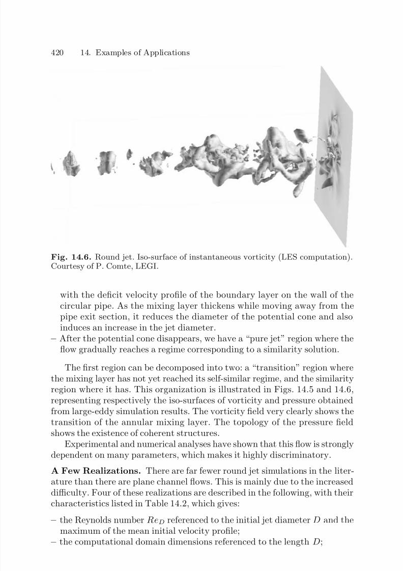
7/21/2019 Large Eddy Simulation for Incompressible Flows
http://slidepdf.com/reader/full/large-eddy-simulation-for-incompressible-flows 438/573
420 14. Examples of Applications
Fig. 14.6. Round jet. Iso-surface of instantaneous vorticity (LES computation).Courtesy of P. Comte, LEGI.
with the deficit velocity profile of the boundary layer on the wall of thecircular pipe. As the mixing layer thickens while moving away from thepipe exit section, it reduces the diameter of the potential cone and alsoinduces an increase in the jet diameter.
– After the potential cone disappears, we have a “pure jet” region where theflow gradually reaches a regime corresponding to a similarity solution.
The first region can be decomposed into two: a “transition” region wherethe mixing layer has not yet reached its self-similar regime, and the similarityregion where it has. This organization is illustrated in Figs. 14.5 and 14.6,
representing respectively the iso-surfaces of vorticity and pressure obtainedfrom large-eddy simulation results. The vorticity field very clearly shows thetransition of the annular mixing layer. The topology of the pressure fieldshows the existence of coherent structures.
Experimental and numerical analyses have shown that this flow is stronglydependent on many parameters, which makes it highly discriminatory.
A Few Realizations. There are far fewer round jet simulations in the liter-ature than there are plane channel flows. This is mainly due to the increaseddifficulty. Four of these realizations are described in the following, with their
characteristics listed in Table 14.2, which gives:
– the Reynolds number ReD referenced to the initial jet diameter D and themaximum of the mean initial velocity profile;
– the computational domain dimensions referenced to the length D;
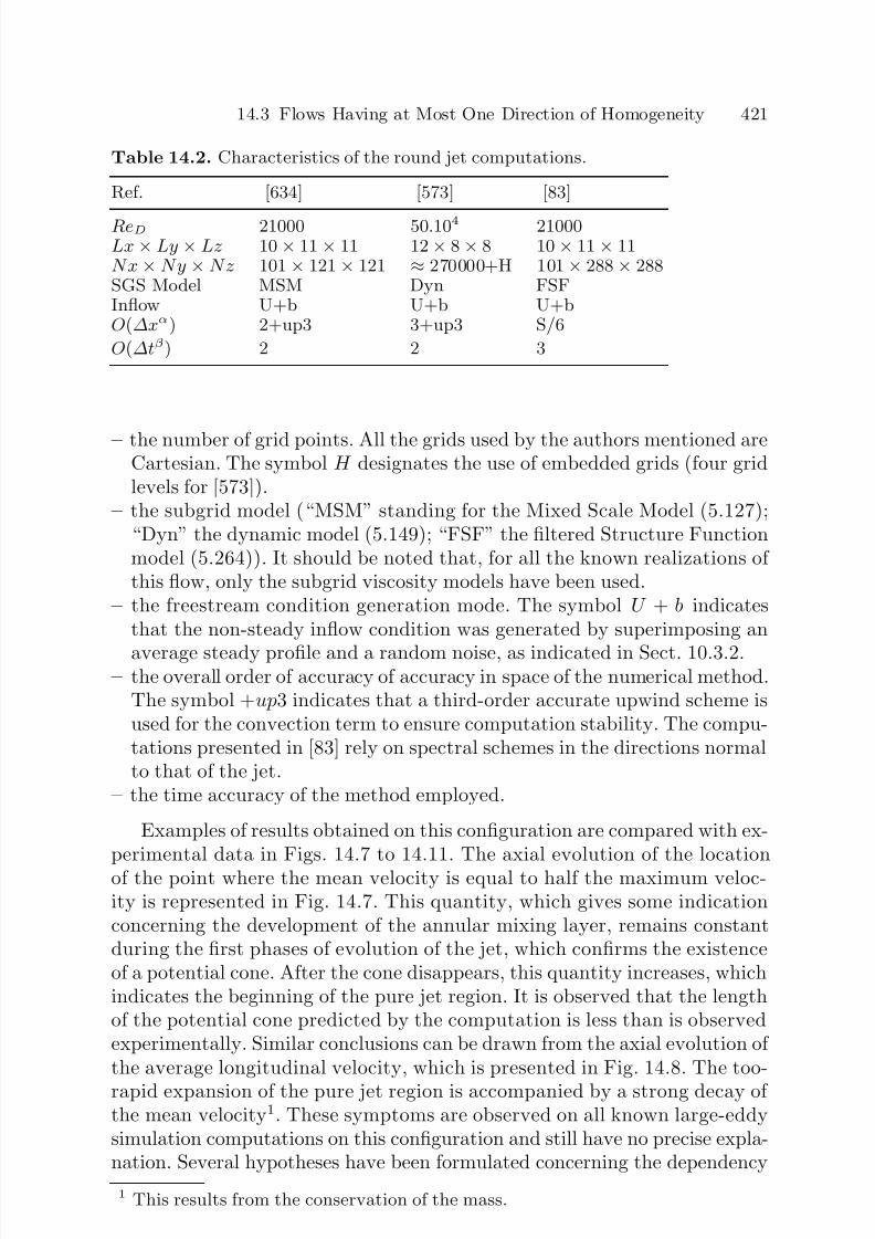
7/21/2019 Large Eddy Simulation for Incompressible Flows
http://slidepdf.com/reader/full/large-eddy-simulation-for-incompressible-flows 439/573
14.3 Flows Having at Most One Direction of Homogeneity 421
Table 14.2. Characteristics of the round jet computations.
Ref. [634] [573] [83]
ReD 21000 50.104 21000Lx × Ly × Lz 10 × 11 × 11 12 × 8 × 8 10 × 11 × 11Nx × Ny × Nz 101 × 121 × 121 ≈ 270000+H 101 × 288 × 288SGS Model MSM Dyn FSFInflow U+b U+b U+bO(∆xα) 2+up3 3+up3 S/6
O(∆tβ) 2 2 3
– the number of grid points. All the grids used by the authors mentioned areCartesian. The symbol H designates the use of embedded grids (four gridlevels for [573]).
– the subgrid model (“MSM” standing for the Mixed Scale Model (5.127);“Dyn” the dynamic model (5.149); “FSF” the filtered Structure Functionmodel (5.264)). It should be noted that, for all the known realizations of this flow, only the subgrid viscosity models have been used.
– the freestream condition generation mode. The symbol U + b indicatesthat the non-steady inflow condition was generated by superimposing an
average steady profile and a random noise, as indicated in Sect. 10.3.2.– the overall order of accuracy of accuracy in space of the numerical method.
The symbol +up3 indicates that a third-order accurate upwind scheme isused for the convection term to ensure computation stability. The compu-tations presented in [83] rely on spectral schemes in the directions normalto that of the jet.
– the time accuracy of the method employed.
Examples of results obtained on this configuration are compared with ex-perimental data in Figs. 14.7 to 14.11. The axial evolution of the locationof the point where the mean velocity is equal to half the maximum veloc-ity is represented in Fig. 14.7. This quantity, which gives some indicationconcerning the development of the annular mixing layer, remains constantduring the first phases of evolution of the jet, which confirms the existenceof a potential cone. After the cone disappears, this quantity increases, whichindicates the beginning of the pure jet region. It is observed that the lengthof the potential cone predicted by the computation is less than is observedexperimentally. Similar conclusions can be drawn from the axial evolution of the average longitudinal velocity, which is presented in Fig. 14.8. The too-
rapid expansion of the pure jet region is accompanied by a strong decay of the mean velocity1. These symptoms are observed on all known large-eddysimulation computations on this configuration and still have no precise expla-nation. Several hypotheses have been formulated concerning the dependency
1 This results from the conservation of the mass.

7/21/2019 Large Eddy Simulation for Incompressible Flows
http://slidepdf.com/reader/full/large-eddy-simulation-for-incompressible-flows 440/573
422 14. Examples of Applications
Fig. 14.7. Round jet. Axial evolution of the radial position of the point wherethe mean velocity is half the maximum velocity. Dots: experimental data. Dot-dashed lines: extrapolation of this data. Solid line: LES computation. Courtesy of P. Comte, LEGI.
Fig. 14.8. Round jet. Axial evolution of the mean longitudinal velocity. Dots:experimental data. Line: LES computation. Courtesy of P. Comte, LEGI.
7/21/2019 Large Eddy Simulation for Incompressible Flows
http://slidepdf.com/reader/full/large-eddy-simulation-for-incompressible-flows 441/573
14.3 Flows Having at Most One Direction of Homogeneity 423
on the initial perturbation, on the boundary conditions, or on the computa-tional grid. The axial profiles of two main Reynolds stresses are presented inFigs. 14.9 and 14.10. These results are qualitatively correct. The Reynoldsstresses increase along the axis and exhibit a maximum in a region close tothe tip of the potential cone, which is in agreement with the experimentalobservations. It is noted that the level of the longitudinal stress predicted bythe computation is higher than the experimental level in the pure jet region.The peak observed on the downstream boundary of the computational do-main is a spurious effect that is no doubt related to the outflow condition.Generally, it is noticed that the quality of the results is not as good as inthe case of the plane channel flow, which illustrates the fact that this flow isa more complicated case for large-eddy simulation.
Lastly, the velocity spectra generated from the computation are presentedin Fig. 14.11. Over a decade, the computations recover a slope close to the−5/3 predicted by theory, and which is the foundation of the theoreticalanalyses presented in the previous chapters. This indicates that the resolvedturbulent scales have “physical” behavior.
More generally, the conclusions given by the various authors are the fol-lowing.
– The dynamics of the numerical solution is consistent, i.e. the values pro-duced are located within the bounds fixed by the collected set of experimen-tal measurements and the topology of the simulated flow exhibits the ex-pected characteristics (potential cone, annular mixing layer, and so forth).
– While the dynamics is consistent, it is nonetheless very difficult to repro-duce a particular realization (for example with fixed potential cone lengthand maximum turbulent intensity).
– The numerical solution exhibits a strong dependency on many parameters,among which we find:– the subgrid model, which allows a more or less rapid transition of the
annular mixing layer are consequently influences the length of the poten-tial cone and the turbulent intensity by modifying the effective Reynoldsnumber in the simulation. More dissipative models delay the develop-ment of the mixing layer, inducing the existence of a very long potentialcone.
– the inflow condition: the mixing layer transition is also strongly depen-dent on the amplitude and shape of the perturbations.
– the numerical error, which can affect the turbulent of the annular mixinglayer and of the developed jet, especially during the transition phases.
Here it is a matter of an error controlled by the computational gridand the numerical method. A dispersive error will have a tendency toaccelerate the transition and thereby shorten the potential cone. A dis-sipative error will have the inverse effect. With too coarse a grid, theannular mixing layer cannot be represented correctly, which can induce
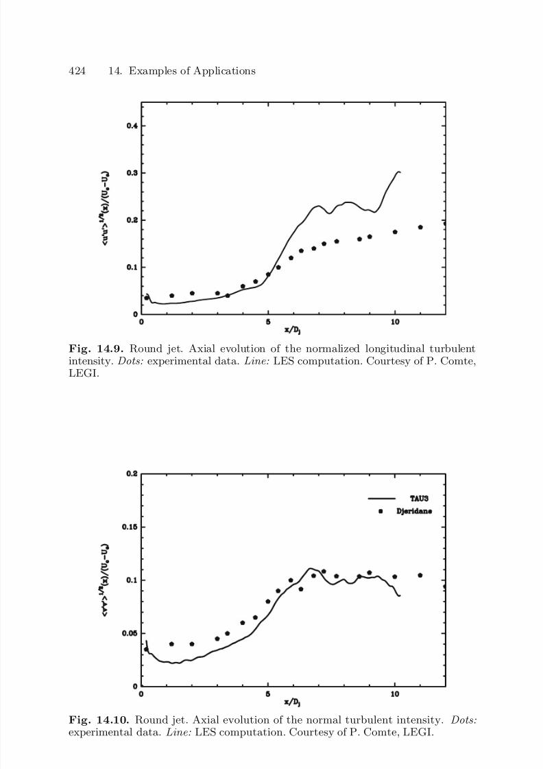
7/21/2019 Large Eddy Simulation for Incompressible Flows
http://slidepdf.com/reader/full/large-eddy-simulation-for-incompressible-flows 442/573
424 14. Examples of Applications
Fig. 14.9. Round jet. Axial evolution of the normalized longitudinal turbulentintensity. Dots: experimental data. Line: LES computation. Courtesy of P. Comte,LEGI.
Fig. 14.10. Round jet. Axial evolution of the normal turbulent intensity. Dots:experimental data. Line: LES computation. Courtesy of P. Comte, LEGI.
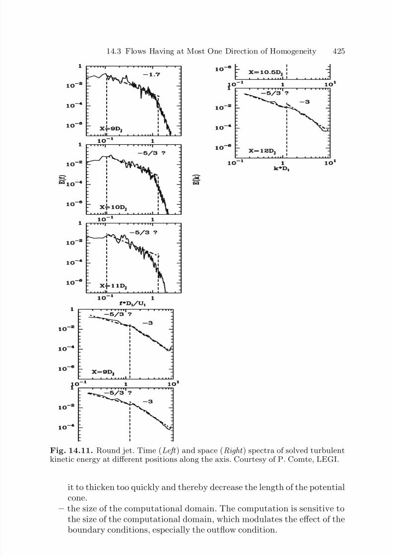
7/21/2019 Large Eddy Simulation for Incompressible Flows
http://slidepdf.com/reader/full/large-eddy-simulation-for-incompressible-flows 443/573
14.3 Flows Having at Most One Direction of Homogeneity 425
Fig. 14.11. Round jet. Time (Left ) and space (Right ) spectra of solved turbulentkinetic energy at different positions along the axis. Courtesy of P. Comte, LEGI.
it to thicken too quickly and thereby decrease the length of the potentialcone.
– the size of the computational domain. The computation is sensitive tothe size of the computational domain, which modulates the effect of theboundary conditions, especially the outflow condition.
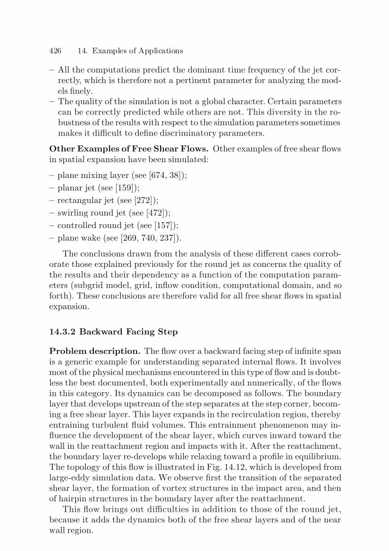
7/21/2019 Large Eddy Simulation for Incompressible Flows
http://slidepdf.com/reader/full/large-eddy-simulation-for-incompressible-flows 444/573
426 14. Examples of Applications
– All the computations predict the dominant time frequency of the jet cor-rectly, which is therefore not a pertinent parameter for analyzing the mod-els finely.
– The quality of the simulation is not a global character. Certain parameterscan be correctly predicted while others are not. This diversity in the ro-bustness of the results with respect to the simulation parameters sometimesmakes it difficult to define discriminatory parameters.
Other Examples of Free Shear Flows. Other examples of free shear flowsin spatial expansion have been simulated:
– plane mixing layer (see [674, 38]);
– planar jet (see [159]);
– rectangular jet (see [272]);
– swirling round jet (see [472]);
– controlled round jet (see [157]);
– plane wake (see [269, 740, 237]).
The conclusions drawn from the analysis of these different cases corrob-orate those explained previously for the round jet as concerns the quality of the results and their dependency as a function of the computation param-
eters (subgrid model, grid, inflow condition, computational domain, and soforth). These conclusions are therefore valid for all free shear flows in spatialexpansion.
14.3.2 Backward Facing Step
Problem description. The flow over a backward facing step of infinite spanis a generic example for understanding separated internal flows. It involvesmost of the physical mechanisms encountered in this type of flow and is doubt-
less the best documented, both experimentally and numerically, of the flowsin this category. Its dynamics can be decomposed as follows. The boundarylayer that develops upstream of the step separates at the step corner, becom-ing a free shear layer. This layer expands in the recirculation region, therebyentraining turbulent fluid volumes. This entrainment phenomenon may in-fluence the development of the shear layer, which curves inward toward thewall in the reattachment region and impacts with it. After the reattachment,the boundary layer re-develops while relaxing toward a profile in equilibrium.The topology of this flow is illustrated in Fig. 14.12, which is developed fromlarge-eddy simulation data. We observe first the transition of the separatedshear layer, the formation of vortex structures in the impact area, and thenof hairpin structures in the boundary layer after the reattachment.
This flow brings out difficulties in addition to those of the round jet,because it adds the dynamics both of the free shear layers and of the nearwall region.
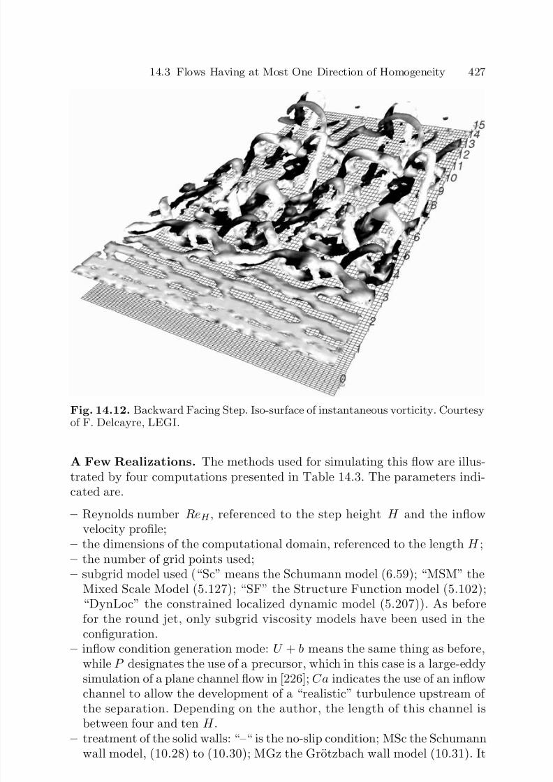
7/21/2019 Large Eddy Simulation for Incompressible Flows
http://slidepdf.com/reader/full/large-eddy-simulation-for-incompressible-flows 445/573
14.3 Flows Having at Most One Direction of Homogeneity 427
Fig. 14.12. Backward Facing Step. Iso-surface of instantaneous vorticity. Courtesyof F. Delcayre, LEGI.
A Few Realizations. The methods used for simulating this flow are illus-trated by four computations presented in Table 14.3. The parameters indi-cated are.
– Reynolds number ReH , referenced to the step height H and the inflowvelocity profile;
– the dimensions of the computational domain, referenced to the length H ;– the number of grid points used;– subgrid model used (“Sc” means the Schumann model (6.59); “MSM” the
Mixed Scale Model (5.127); “SF” the Structure Function model (5.102);“DynLoc” the constrained localized dynamic model (5.207)). As beforefor the round jet, only subgrid viscosity models have been used in theconfiguration.
– inflow condition generation mode: U + b means the same thing as before,while P designates the use of a precursor, which in this case is a large-eddysimulation of a plane channel flow in [226]; Ca indicates the use of an inflowchannel to allow the development of a “realistic” turbulence upstream of the separation. Depending on the author, the length of this channel isbetween four and ten H .
– treatment of the solid walls: “–“ is the no-slip condition; MSc the Schumannwall model, (10.28) to (10.30); MGz the Grotzbach wall model (10.31). It

7/21/2019 Large Eddy Simulation for Incompressible Flows
http://slidepdf.com/reader/full/large-eddy-simulation-for-incompressible-flows 446/573
428 14. Examples of Applications
Table 14.3. Backward facing step computation characteristics.
Ref. [226] [637] [673] [261]
ReH 1, 65.105 11200 38000 28 000Lx × Ly × Lz 16 × 4 × 2 20 × 4 × 2, 5 30 × 5 × 2, 5 30 × 3 × 4N x × N y × Nz 128 × 32 × 32 201 × 31 × 51 200 × 30 × 30 244 × 96 × 96SGS Model Sc MSM FS DynLocInflow P U+b U+b U+b,CaWall MSc – MLog –O(∆xα) 2 2+up3 2+up3 2
O(∆tβ) 2 2 2 3
can be seen that the use of wall models reduces the number of pointsconsiderably and makes it possible to simulate flows with high Reynoldsnumbers.
– spatial accuracy of the numerical method;– time accuracy of the numerical method.
The results the various authors have obtained are generally in good qual-itative agreement with experimental data: the flow topology is recovered andthe realizations show the existence of coherent structures similar to thoseobserved in the laboratory. On the other hand, there is much more difficultyobtaining quantitative agreement whenever this is possible at all (only ref-erence [261] produces results in satisfactory agreement on the mean velocityfield and turbulent intensity). This is due to the very high sensitivity of theresult to the computation parameters. For example, variations of the orderof 100% of the average length of the recirculation region have been recordedwhen the inflow boundary condition or subgrid model are manipulated. Thissensitivity stems from the fact that the flow dynamics is governed by thatof the separated shear layer, so the problems mentioned before concerning
free shear flows crop up here. We also note a tendency to under-estimate thevalue of the mean velocity in the recirculation area. However, as in the caseof the round jet, the simulated physics does correspond to that of a backwardfacing step flow. This is illustrated by the mean velocity profiles and resolvedReynolds stresses in Fig. 14.13, and the pressure spectra in Fig. 14.14. Thegood agreement with experimental data in the prediction of the mean fieldand Reynolds stresses proves the theoretical consistency of the computa-tion. This agreement is even clearer if we analyze the spectra. Near the step,the mixing layer dynamics is dominated by frequencies associated with the
Kelvin-Helmholtz instability. The predicted value of the dominant frequencyis in very good agreement with experimental observations. The double peakat the second measurement point shows that the simulation is capable of re-flecting the low-frequency flapping mechanism of the separated region, andstill remain in good agreement with experimental observations.

7/21/2019 Large Eddy Simulation for Incompressible Flows
http://slidepdf.com/reader/full/large-eddy-simulation-for-incompressible-flows 447/573
14.3 Flows Having at Most One Direction of Homogeneity 429
Fig. 14.13. Backward Facing Step. Mean velocity and Reynolds stresses profilesat the reattachment point. Triangles and solid line: LES computations. Squares:experimental data. Courtesy of F. Delcayre, LEGI.
Fig. 14.14. Backward Facing Step. Pressure spectra. Squares: in the free shearlayer near the step corner. Triangles: in the separated region near the reattachmentpoint. Courtesy of F. Delcayre, LEGI.
Also, it seems that the use of wall models does not affect the dynamicsof this shear layer greatly. It becomes possible to deal with higher Reynolds
numbers, but at the price of losing some of the quality of the results as con-cerns the wall surface terms (friction, pressure coefficient) in the recirculationzone [87]. Solutions for this configuration turn out to be highly dependent onthe subgrid model: a too dissipative model will delay the development of theseparated shear layer, pushing away the position of the reattachment point.
7/21/2019 Large Eddy Simulation for Incompressible Flows
http://slidepdf.com/reader/full/large-eddy-simulation-for-incompressible-flows 448/573
430 14. Examples of Applications
The results are also found to be dependent on the size of the domain andthe fineness of the mesh in the spanwise direction, because these parametersaffect the development of the mixing layer emanating from the step corner.A spanwise domain width of 4 to 6 H is considered to be a minimum in orderto be able to capture the three-dimensional mechanisms at low frequencies.Lastly, the time frequencies associated with the separated zone dynamics arerobust parameters in the sense that they are often predicted with precision.
14.3.3 Square-Section Cylinder
Problem description. The square-section infinite-span cylinder is a goodexample of separated external flows around bluff bodies. This type of configu-ration involves phenomena as diversified as the impact of the flow on a body,its separation (and possible reattachment) on the body surface, the formationof a near-wake region, and alternating vortex street, and the development of the wake up to a self-similar solution. Each of these phenomena poses its ownparticular numerical and modeling problems.
Realizations. This flow was chosen as an international test case for large-eddy simulation, and has consequently served as a basis for many compu-tations, which are mostly summarized in [618] (see also [555, 729, 730, 678,
233, 94, 652] for a discussion of this test case). The test case parameters are:a Reynolds number ReD, referenced to the length D of the cylinder edgeand the freestream velocity, equal to 22,000, and a computational domainof 20D × 4D × 14D. The span is assumed to be infinite and a periodicitycondition is used in this direction.
None of the sixteen computations collected in [618] produces an overallgood agreement with experimental data, i.e. is capable of predicting all of thefollowing parameters with an error of less than 30%: average lift and drag;drag and lift variances; main vortex shedding frequency; and average length
of the separated region behind the cylinder. Average lift and drag, as wellas the vortex shedding frequency, are very often predicted very satisfactorily.This is due to the fact that these quantities do not depend on the smallscale turbulence and are governed by Von Karman structures, which are verylarge in size. The length of the recirculation region behind the cylinder isvery often under-estimated, as is the amplitude of the mean velocity in thisregion. Also, the mean velocity in the wake is only very rarely in agreementthe experimental data.
The numerical methods used are of moderate order of accuracy (atmost second-order in space and third-order in time), and third-order up-wind schemes are often used for the convection term. Only subgrid viscositymodels have been used (Smagorinsky model, various dynamic models, MixedScale Model). Certain authors use wall models at the cylinder surface.
The lack of agreement with experimental data is explained by the veryhigh sensitivity of the different driving mechanisms to the numerical errors

7/21/2019 Large Eddy Simulation for Incompressible Flows
http://slidepdf.com/reader/full/large-eddy-simulation-for-incompressible-flows 449/573
14.3 Flows Having at Most One Direction of Homogeneity 431
and to the diffusion introduced by the models. So we again find here the prob-lems mentioned above for the case of the backward facing step, but now theyare amplified by the fact that, in order to master the impact phenomenonnumerically, the numerical diffusion introduced is much stronger than in theformer case. Also, as most of the grids used are Cartesian and monodomain,the resolution near the cylinder is too weak to allow a satisfactory represen-tation of the boundary layers.
14.3.4 Other Examples
Many other flows have been examined by large-eddy simulation.Among wall-bounded flows without separation, we may mention: flat plate
boundary layer [237, 205, 463, 457, 585]; boundary layer on a curved sur-face in the presence of Gortler vortices [460]; flow in a circular-section toricpipe [653]; three-dimensional boundary layer [767, 366]; juncture flow [687];flow in a rotating pipe [777, 215]; flow in a rotating square duct [576]; flowin a square/rectangular annular duct [774, 65].
Examples of recirculating flows are: confined coaxial round jets [9]; flowaround a wing section of infinite span at incidence [347, 371, 348, 349, 425,78, 502, 494] (see Fig. 14.15); flow in a planar asymmetric diffuser [367,213, 372, 369]; flow around a cube mounted on a flat plate [618, 556, 757,
493, 652, 407]; flow around a circular-section cylinder [52, 519, 520, 362,75, 410, 715, 77, 360, 76]; flow in tube bundles [620]; flow in a lid-drivencavity [799, 179]; flow in a ribbed channel/duct [779, 142, 778, 151, 361]; jet
Fig. 14.15. Flow around a wing at high incidence: isosurface of instantaneousvorticity. Courtesy of R. Lardat and L. Ta Phuoc, LIMSI.

7/21/2019 Large Eddy Simulation for Incompressible Flows
http://slidepdf.com/reader/full/large-eddy-simulation-for-incompressible-flows 450/573
432 14. Examples of Applications
impacting a flat plate [739, 616, 574, 51, 718]; boundary layer on a wavysurface or a bump [412, 197, 770, 302, 768, 769, 642, 522]; flow over a sweptwedge [330]; flow past a blunt trailing edge [484, 754, 564, 571]; separatedboundary layer [88, 758]; aircraft wake vortices [286]; axisymmetric piston-cylinder flow [732]; flow around an oscillating cylinder [721]; flow arounda road vehicle [731, 408]; flow around a 3D wing [329]; flow around a squarecylinder [399, 393]; flow around a forward-backward facing step [5]; flow inreversing systems [61]; flow in a blade passage [147, 516]; flow pas a sweptfence [178]; flow over a sphere [146].
14.4 Industrial Applications
14.4.1 Large-Eddy Simulation for Nuclear Power Plants
The increasing power of supercomputers and of numerical description of un-steady flows allows the simulation of complex flows relevant to industrialconfigurations in accident scenarios obviously not available through experi-ments. Simulation is used to capture large features of the flow and to focus onmajor events, at least concerning qualitative behavior. The present exampledeals with induced rupture of the primary circuit in a pressurized water reac-
tor. The simulation domain includes the reactor vessel, the steam generatorand their connection through the hot leg (see Fig. 14.16): the dimensions of the real domain cover several meters. For the calculation, the steam genera-tor tubes have been grouped into nine, thus decreasing the number of controlvolumes (a model has been developed to take into account this change in thegeometry). Furthermore, the tube’s length has been reduced in order to limitthe computer time consumption.
In the case of the total loss of the heat sink (very hypothetical severe ac-cident scenario) the flow circulation driven by the primary pump is stopped,
the coolant is pure vapour (T > 1000 C) and natural convection develops inthe circuit. The question here is to investigate the temperature distributionin the wall of the hot leg and in the tubes of the steam generator, in orderto analyze their mechanical constraints. For that it is crucial to get the bestdiscretization of the related zones. This is achieved by concentrating the gridpoints in this area. Figure 14.16 shows the mesh of each tube of a “simplifiedsteam generator” composed of 400 tubes (3300 in reality). Figure 14.17 (top)provides a global view of the flow in the hot leg, showing a clear stratificationand a return of flow into the core. Figure 14.17 (bottom) displays a cut in the
hot leg at different locations, showing an increase of turbulence and mixingas the section is closer to the steam generator: this mixing leads to homoge-nization of the temperature and reduced mechanical constraints. The presentsimulation was performed using the TRIO-U/PRICELES code developed atCEA Grenoble (in the DTP/SMTH/LDTA laboratory): it required around106 grid points using a tetrahedral discretization. The underlying numerical

7/21/2019 Large Eddy Simulation for Incompressible Flows
http://slidepdf.com/reader/full/large-eddy-simulation-for-incompressible-flows 451/573
14.4 Industrial Applications 433
Fig. 14.16. Top: global view of the unstructured mesh. A coarse discretization ischosen for the vessel, taking into account here a realistic boundary condition . Theresolution is finer in a region of interest, say the steam generator region (tubes andplenum). Bottom : local view of the mesh of the steam generator: 400 individualtubes are independently meshed. Courtesy of IRSN.

7/21/2019 Large Eddy Simulation for Incompressible Flows
http://slidepdf.com/reader/full/large-eddy-simulation-for-incompressible-flows 452/573
434 14. Examples of Applications
Fig. 14.17. Top: a cut in the instantaneous temperature field in the whole system,showing a stratification in the “hot leg” that propagates in the direction of thesteam generator tubes; a back flow develops in the vessel. Bottom : cuts of the samefield near the steam generator, plus velocity vectors. Stratification is perturbatedby the turbulent flow. Courtesy of IRSN.
method is a centered second-order accurate Finite Element based discretiza-tion, used together with a standard Smagorinsky model. All simulations wereperformed by U. Bieder (CEA) and H. Mutelle (IRSN) for the French NuclearSafety Institute (IRSN).

7/21/2019 Large Eddy Simulation for Incompressible Flows
http://slidepdf.com/reader/full/large-eddy-simulation-for-incompressible-flows 453/573
14.4 Industrial Applications 435
For other situations where experimental data are available, qualitative aswell as quantitative features are looked at, as in more traditional disciplines.
14.4.2 Flow in a Mixed-Flow Pump
This example of the use of large-eddy simulation for turbomachinery flowsis due to C. Kato et al. [380]. These authors computed the internal flow ina mixed-flow pump stage with a high designed specific speed.
A view of the computational domain is shown in Fig. 14.18. The compu-tational domain includes: the upstream inlet pipe, the two regulation plates,a four-blade impeller and the diffuser, leading to a very complex configura-tion, both from the geometrical and physical points of view.
In order to take the rotation into account, the authors make use of a Chimera-type technique: a moving boundary interface in the flow field istreated with overset grids from multiple frames of reference. A computationalgrid that rotates along with the impeller is used to compute the flow withinthe impeller, and stationary grids are used for stationary parts of the pump.Each grid includes appropriate margins of overlap with its neighboring gridsin order to allow appropriate interpolations, and coordinate transformationto take into account the different frames of reference.
Two mesh resolutions have been investigated: a coarse grid with a totalof 1.7 × 10⁶ points and a fine grid with 5 × 10⁶ points. A partial view of thesurface mesh on the impeller is shown in Fig. 14.19. The boundary conditionsare the following: no-slip boundary conditions are used on solid walls, andthe turbulent pipe flow at the inlet is obtained by performing an auxiliarylarge-eddy simulation of an infinite pipe flow.
Fig. 14.18. Flow in a mixed-flow pump. View of the global computational domain.Courtesy of C. Kato, University of Tokyo.

7/21/2019 Large Eddy Simulation for Incompressible Flows
http://slidepdf.com/reader/full/large-eddy-simulation-for-incompressible-flows 454/573
436 14. Examples of Applications
Fig. 14.19. Partial view of the surface mesh. Courtesy of C. Kato, University of Tokyo.
A classical Smagorinsky model is employed, with a Van Driest damp-ing function enforcing a vanishing subgrid viscosity in the near-wall region.A streamwise-upwind finite-element method is used to discretize the Navier–Stokes equations. Time integration is based on the explicit Euler scheme,but shifts the spatial residuals of the governing equations in the upstreamdirection of the local flow. The magnitude of this shift is one half of the timeincrement multiplied by the magnitude of the local flow velocity, yieldingan exact cancellation of the first-order error terms. The resulting method is
second-order accurate in space and time.Several operating conditions of the pump have been investigated using
large-eddy simulations. All of them correspond to partial load conditions, i.e.off-design operating conditions.
Comparison of computed and measured head-flow characteristics is shownin Fig. 14.20, showing a very good agreement between fine-grid simulationsand experiments. Coarse grid simulation is seen to yield larger discrepancieswhen design operating conditions are approached, because the mesh is notfine enough to capture accurately the attached boundary-layer dynamics. The
normalized head-flow characteristic is defined here as the relation between theflow-rate of the pump and its total-pressure rise. After stall onset (Q/Qd ≤0.55, where Q is the mass flowrate), both grids yield very similar descriptionsof the flow. As in the previous case, Qd is the mass flow-rate related to thedesign point.
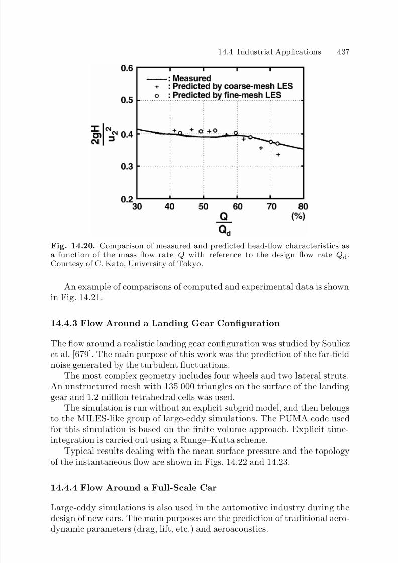
7/21/2019 Large Eddy Simulation for Incompressible Flows
http://slidepdf.com/reader/full/large-eddy-simulation-for-incompressible-flows 455/573
14.4 Industrial Applications 437
Fig. 14.20. Comparison of measured and predicted head-flow characteristics asa function of the mass flow rate Q with reference to the design flow rate Qd.Courtesy of C. Kato, University of Tokyo.
An example of comparisons of computed and experimental data is shown
in Fig. 14.21.
14.4.3 Flow Around a Landing Gear Configuration
The flow around a realistic landing gear configuration was studied by Souliezet al. [679]. The main purpose of this work was the prediction of the far-fieldnoise generated by the turbulent fluctuations.
The most complex geometry includes four wheels and two lateral struts.An unstructured mesh with 135 000 triangles on the surface of the landing
gear and 1.2 million tetrahedral cells was used.The simulation is run without an explicit subgrid model, and then belongs
to the MILES-like group of large-eddy simulations. The PUMA code usedfor this simulation is based on the finite volume approach. Explicit time-integration is carried out using a Runge–Kutta scheme.
Typical results dealing with the mean surface pressure and the topologyof the instantaneous flow are shown in Figs. 14.22 and 14.23.
14.4.4 Flow Around a Full-Scale Car
Large-eddy simulations is also used in the automotive industry during thedesign of new cars. The main purposes are the prediction of traditional aero-dynamic parameters (drag, lift, etc.) and aeroacoustics.

7/21/2019 Large Eddy Simulation for Incompressible Flows
http://slidepdf.com/reader/full/large-eddy-simulation-for-incompressible-flows 456/573
438 14. Examples of Applications
Fig. 14.21. Predicted and measured phase-averaged velocity profiles at the im-peller’s inlet cross-section for Q/Qd = 0.43 (post-stall operating condition). Cour-tesy of C. Kato, University of Tokyo.
The example presented here deals with the large-eddy simulations of theflow around a full-scale car model. The wheels and the floor are fixed, as inthe wind tunnel experiments. The Reynolds number is 2 684 563 per meter.
The numerical simulation is carried out using the Powerflow code, whichis based on the Lattice Boltzmann approach (see [127] for an introduction).A Cartesian grid is used, which is composed of 20 × 106 cells. The size of thesmallest mesh is 7 mm. Subgrid scales are taken into account using a two-equation k − τ subgrid model. A wall model is used at solid boundaries.
Fig. 14.22. Predicted mean surface pressure on the landing gear. Courtesy of F. Souliez and L. Long, Pennsylvania State University.

7/21/2019 Large Eddy Simulation for Incompressible Flows
http://slidepdf.com/reader/full/large-eddy-simulation-for-incompressible-flows 457/573
14.5 Lessons 439
Fig. 14.23. Instantaneous vorticity filaments. Courtesy of F. Souliez and L. Long,Pennsylvania State University.
Typical results are displayed in Figs. 14.24–14.27. The very complex topol-ogy of the flow is recovered, exhibiting very intense vortical structures andpressure variations. The drag is predicted to be within 1% error in comparisonwith experimental data.
14.5 Lessons
14.5.1 General Lessons
We can draw the following lessons concerning the large-eddy simulation tech-nique from the computations mentioned above:
– When the technique is used for dealing with the ideal case in which it wasderived (homogeneous turbulence, optimal numerical method), it yieldsvery good results. The vast majority of subgrid models produce results thatare indiscernable from reality, which removes any discriminatory characterfrom this type of test case, which in fact can only be used to assess theconsistency of the method.
– Extending the technique to inhomogeneous cases brings up many otherproblems, concerning both the physical modeling (subgrid models) andthe numerical method. The latter point becomes crucial because the use of
numerical methods of moderate order of accuracy (generally two) greatlyincreases the effect of the numerical error. This is accentuated by the use of artificial dissipations for stabilizing the simulation in “stiff” cases (strongunder-resolution, strong gradients). This error seems to be reducable byrefining the computational grid, which is done more and more by usingadaptive grids (local adaptation or enrichment).
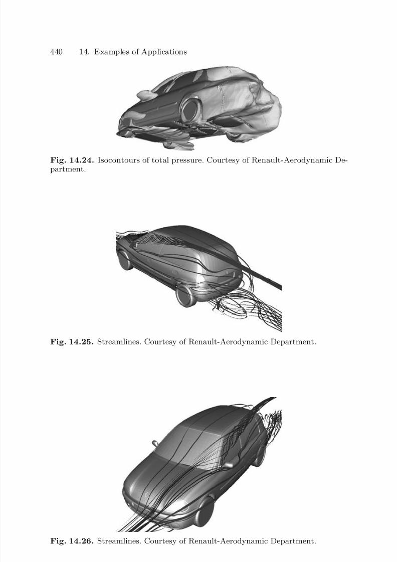
7/21/2019 Large Eddy Simulation for Incompressible Flows
http://slidepdf.com/reader/full/large-eddy-simulation-for-incompressible-flows 458/573
440 14. Examples of Applications
Fig. 14.24. Isocontours of total pressure. Courtesy of Renault-Aerodynamic De-partment.
Fig. 14.25. Streamlines. Courtesy of Renault-Aerodynamic Department.
Fig. 14.26. Streamlines. Courtesy of Renault-Aerodynamic Department.

7/21/2019 Large Eddy Simulation for Incompressible Flows
http://slidepdf.com/reader/full/large-eddy-simulation-for-incompressible-flows 459/573
14.5 Lessons 441
Fig. 14.27. Streamlines. Courtesy of Renault-Aerodynamic Department.
– Shear flows show themselves to be very strongly dependent on the inflowcondition when this is unsteady. Generating these conditions is still anopen problem.
– The quality of the results is variable but, for each configuration, robust,correctly predicted parameters exist. The physics simulated is often consis-tent in that it exhibits the generic features that are observed experimentallybut does not necessarily correspond to a desired target realization. This is
due to the dependency on the many simulation parameters.– The quality of the results is subordinate to the correct representation of the flow driving mechanisms (transition, near-wall dynamics, and so forth).Low numerical error and consistent modeling are therefore mandatory inthose regions where these mechanisms occur. The other regions of the flowwhere the energy cascade is the dominant mechanism are of lesser impor-tance.
– When the flow dynamics becomes complex, subgrid viscosity models areoften used. This is because they provide a clear kinetic energy dissipationand therefore stabilize the simulation. This stabilizing character seems tobecome predominant compared with the physical quality of the modelinginsofar as the numerical difficulties increase (with the presence of strongshear and highly heterogeneous grids, and so forth).
– There is a consensus today that the numerical method used must be accu-rate to at least the second order in space and time. First-order accurate nu-merical dissipations are totally proscribed. Third-order accurate methodsin time are rarely used. As concerns the spatial accuracy, satisfactory re-sults are obtained by certain authors with second-order accurate methods,but higher-order accurate schemes are often used. Numerical stabilization
methods (upwind scheme, artificial dissipation, smoothing, and so forth)should be used only when absolutely necessary.
– Large-eddy simulation is presently a powerful tool for investigating mas-sively separated industrial flows, where the large scales and the turbulenceproduction is not driven by fine details of the dynamics of the boundary

7/21/2019 Large Eddy Simulation for Incompressible Flows
http://slidepdf.com/reader/full/large-eddy-simulation-for-incompressible-flows 460/573
442 14. Examples of Applications
layers. For other flows, such as fully attached flows, large-eddy simulationis still too expensive to be used on full-scale configurations for realisticReynolds numbers because of the huge number of grid points required toobtain an accurate resolution of the boundary layers. Existing wall modelshave not been validated in realistic cases up to now, and the question of their validity for such flows remains an open question.
14.5.2 Subgrid Model Efficiency
Here we will try to draw some conclusions concerning the efficiency of thesubgrid models for processing a few generic flows. These conclusions should betaken with caution. As we have seen all through this book, very many factors(numerical method, grid, subgrid model, and others) are involved and arealmost indissociable, so it is very difficult to try to isolate the effect of a modelin a simulation. The conclusions presented are statistical in the sense thatthey are the fruit of an analysis of simulations performed on similar (at leastgeometrically) flow configurations with different methods. A “deterministic”analysis could lead to contradictory conclusions, depending on the other.Also, there is no question of ranking the models, as the available informationis too lacunary to draw up a reliable list. Lastly, very many factors like thediscretization of the subgrid models still remain to be studied.
We may, however, sketch out the following conclusions.
1. To simulate a homogeneous flow:a) All subgrid models including a subgrid viscosity yield similar results.
The efficiency of functional models for the forward energy cascadein isotropic turbulence, despite their lack of accuracy in representingthe subgrid tensor eigenvectors, was analyzed by Jimenez [351]. It isexplained by the existence of a feedback between the resolved scalesand the net energy drain provided by the subgrid model. Errors in
subgrid models are localized at the highest resolved frequency, anddo not contaminate the low frequency which is responsible for theturbulence production. The error accumulation at high frequenciesleads to an adjustment of the subgrid model, which is expressed asa function of the resolved scales. This is easily seen by writing theinduced subgrid dissipation: ε = −τ ijS ij = 2ν sgs|S |2. A classicalexample is the Smagorinsky model, which leads to ε = C S|S |3. A localunderestimation of C S will result in an energy accumulation at thecutoff, leading to an increase of the resolved shear |S | and an increaseof the net drain of kinetic energy. This drain mostly affects the highestresolved frequencies, leading to a decrease of |S |. The global effecton the flow is small, because the highest resolved frequencies containa small part of the total resolved kinetic energy. The efficiency of this adjustment depends of course on the way the subgrid viscosityis computed.

7/21/2019 Large Eddy Simulation for Incompressible Flows
http://slidepdf.com/reader/full/large-eddy-simulation-for-incompressible-flows 461/573
14.5 Lessons 443
For anisotropic flows the loss of efficiency of the basic subgrid vis-cosity models is a well recognized fact. This is explained by the factthat the shear magnitude
|S |
is not governed by the highest resolvedfrequency any more, but by very large scales. Thus, the dynamic feed-back loop described above is not sufficient any more to yield good re-sults. Self-adaptive models (dynamic, filtered, selective, etc.) must beused to ensure the quality of the results. The available experimentaldata suggest that the correlation obtained using the subgrid-viscositymodel is of the order of 20%. This implies that it is impossible to getboth the right energy spectrum and the right stresses from a subgrid-viscosity model if its effect on the resolved field is not negligible.Grid refinement is known to yield improved results for two reasons:
the error is commited on a smaller fraction of the total kinetic en-ergy, and the Kolmogorov theory predicts that the small scales aremore isotropic than the large ones, rendering the structural errorless important. For a weak shear S , the Kolmogorov theory leads tothe following scaling laws for the normal-stresses spectrum E 11 andoff-diagonal stress cospectrum E 12:
E 11 ∝ ε2/3k−5/3, E 12 ∝ Sε1/3k−7/3 ,
and τ 12 ∝ (πLS/∆)−4/3, τ 12/τ 11 ∝ (πLS/∆)−2/3 ,
where the shear length LS =
ε/S 3 is proportional to the integralscale Lε in equilibrium flows. These scaling laws show that refiningthe resolution, i.e. decreasing ∆, makes it possible to reduce quicklythe anisotropy of the subgrid scales. Jimenez estimates that 1% erroris obtained for Lε/∆ = 10–20.
b) Scale similarity or soft-deconvolution-type models do not yield goodresults if used alone. This is also true for all the other types of flows.
A possible explanation for the improvement observed when usingmixed models or explicit random models for the backward energycascade is that these models weaken the spurious correlation betweenthe resolved strain rate tensor and the modeled subgrid tensor. Thisimprovement is also expected from theoretical results dealing withthe full deconvolution problem or the rapid/slow decomposition in-troduced by Shao et al. It is important to note that on very coarsegrids mixed models may not result in improved results.
c) These results hold locally for all other flows.
2. To simulate a free shear flow (mixing layer, jet, wake):a) Subgrid viscosity models based on large scales can delay the transi-tion. This problem can be remedied by using a dynamic procedure,a selection function, or an accentuation technique. The other subgridviscosity models seem to allow the transition without any harmful ef-fects.
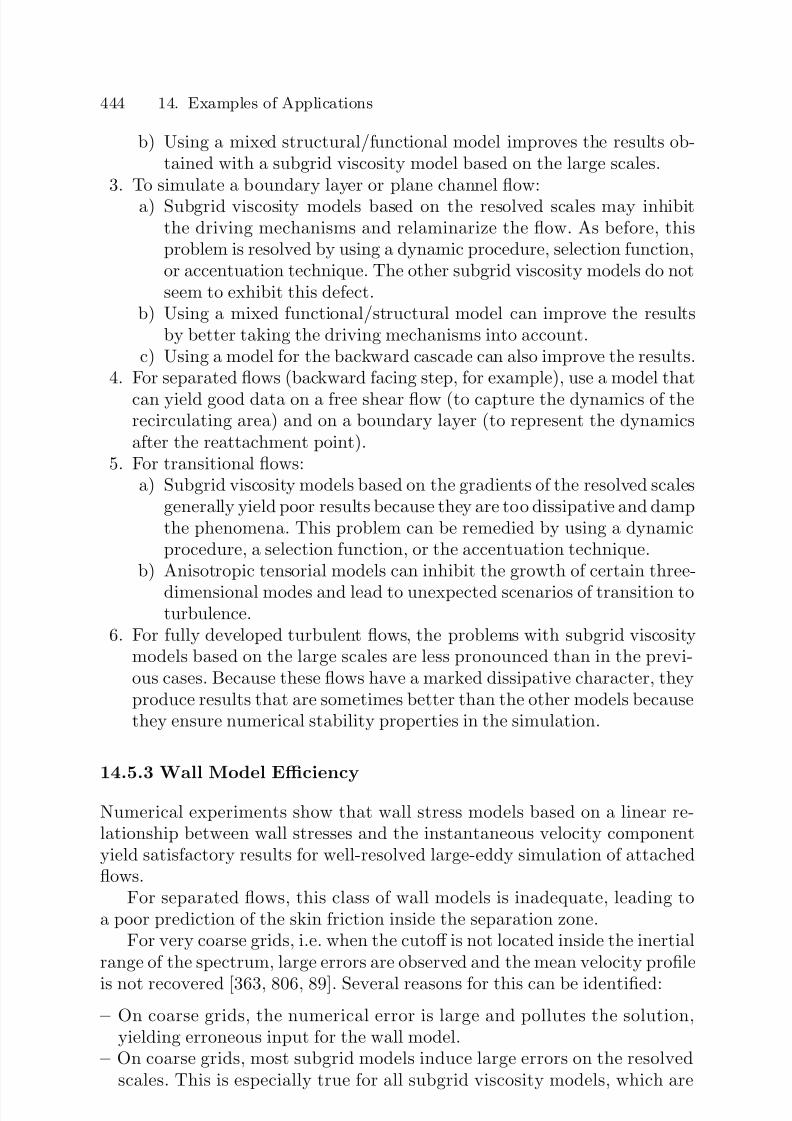
7/21/2019 Large Eddy Simulation for Incompressible Flows
http://slidepdf.com/reader/full/large-eddy-simulation-for-incompressible-flows 462/573
444 14. Examples of Applications
b) Using a mixed structural/functional model improves the results ob-tained with a subgrid viscosity model based on the large scales.
3. To simulate a boundary layer or plane channel flow:a) Subgrid viscosity models based on the resolved scales may inhibit
the driving mechanisms and relaminarize the flow. As before, thisproblem is resolved by using a dynamic procedure, selection function,or accentuation technique. The other subgrid viscosity models do notseem to exhibit this defect.
b) Using a mixed functional/structural model can improve the resultsby better taking the driving mechanisms into account.
c) Using a model for the backward cascade can also improve the results.4. For separated flows (backward facing step, for example), use a model that
can yield good data on a free shear flow (to capture the dynamics of therecirculating area) and on a boundary layer (to represent the dynamicsafter the reattachment point).
5. For transitional flows:a) Subgrid viscosity models based on the gradients of the resolved scales
generally yield poor results because they are too dissipative and dampthe phenomena. This problem can be remedied by using a dynamicprocedure, a selection function, or the accentuation technique.
b) Anisotropic tensorial models can inhibit the growth of certain three-
dimensional modes and lead to unexpected scenarios of transition toturbulence.
6. For fully developed turbulent flows, the problems with subgrid viscositymodels based on the large scales are less pronounced than in the previ-ous cases. Because these flows have a marked dissipative character, theyproduce results that are sometimes better than the other models becausethey ensure numerical stability properties in the simulation.
14.5.3 Wall Model Efficiency
Numerical experiments show that wall stress models based on a linear re-lationship between wall stresses and the instantaneous velocity componentyield satisfactory results for well-resolved large-eddy simulation of attachedflows.
For separated flows, this class of wall models is inadequate, leading toa poor prediction of the skin friction inside the separation zone.
For very coarse grids, i.e. when the cutoff is not located inside the inertialrange of the spectrum, large errors are observed and the mean velocity profile
is not recovered [363, 806, 89]. Several reasons for this can be identified:
– On coarse grids, the numerical error is large and pollutes the solution,yielding erroneous input for the wall model.
– On coarse grids, most subgrid models induce large errors on the resolvedscales. This is especially true for all subgrid viscosity models, which are

7/21/2019 Large Eddy Simulation for Incompressible Flows
http://slidepdf.com/reader/full/large-eddy-simulation-for-incompressible-flows 463/573
14.5 Lessons 445
not able to account for the strong flow anisotropy in the near-wall region.It has been shown [363, 806] that this error is mainly due to the fact thatthe subgrid acceleration term in the filtered momentum equations is notproperly predicted on very coarse grids.2 This bad prediction can lead tothe occurrence of spurious coupling with linear wall models, yielding verybad results. The use of dynamic models may result in worse results if thetest filter is applied outside the inertial range [89].
A very important conclusion of studies dealing with suboptimal-basedwall models is that predicting the mean velocity profile and recovering thebest possible rms velocity profile seem to be competing objectives.
Wall models based on auxiliary simulations performed on secondary em-
bedded grids (RANS, thin boundary layer equations) may be an alternative,which remains to be assessed in critical situations. The use of more com-plex subgrid models, at least in the resolved near-wall region, which are ableto predict the subgrid acceleration is also expected to improve the responseof wall stress models. Multilevel subgrid models have demonstrated a clearsuperiority in academic test cases.
14.5.4 Mesh Generation for Building Blocks Flows
We discuss here the basic rules for mesh generation for two classical building blocks of complex flows, namely the attached equilibrium boundary layer andthe plane mixing layer.
The two basic rules are:
– The key idea is that the driving mechanisms, i.e. the events responsiblefor turbulence production and mean profile instabilities, must be correctlycaptured by the simulation to recover reliable results.
– The size of the computational domain must be larger than the correlationlength of the fluctuations, in each direction of space. Too small a domain
size will yield spurious coupling between the dynamics of the flow and theboundary conditions.
Exact values of mesh size, number of grid points and their repartition,and domain size for ‘plug and play’ simulations are not available: these pa-rameters depend on many parameters, including numerical methods. Whatare presented below are the commonly accepted ideas underlying the designof a large number of published works.
Equilibrium Boundary Layer. As discussed in Sect. 10.2, the boundary
layer exhibits two different scalings.– In the inner layer the viscous length lτ is relevant to describe the dynam-
ics. The typical correlation lenghts are 1000 wall units in the streamwise
2 It is recalled that subgrid viscosity models are designed to yield the correctamount of dissipation, not the proper subgrid acceleration.
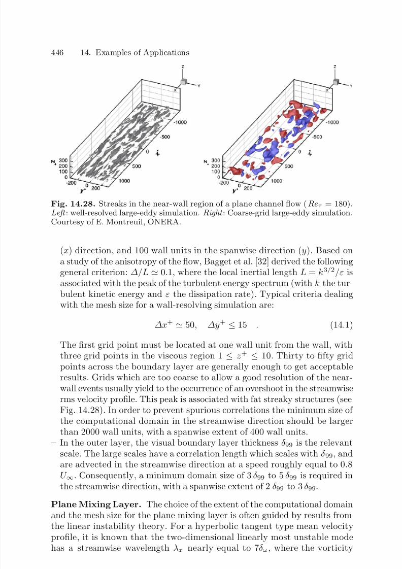
7/21/2019 Large Eddy Simulation for Incompressible Flows
http://slidepdf.com/reader/full/large-eddy-simulation-for-incompressible-flows 464/573
446 14. Examples of Applications
Fig. 14.28. Streaks in the near-wall region of a plane channel flow (Reτ = 180).Left : well-resolved large-eddy simulation. Right : Coarse-grid large-eddy simulation.Courtesy of E. Montreuil, ONERA.
(x) direction, and 100 wall units in the spanwise direction (y). Based ona study of the anisotropy of the flow, Bagget et al. [32] derived the followinggeneral criterion: ∆/L 0.1, where the local inertial length L = k3/2/ε isassociated with the peak of the turbulent energy spectrum (with k the tur-bulent kinetic energy and ε the dissipation rate). Typical criteria dealingwith the mesh size for a wall-resolving simulation are:
∆x+ 50, ∆y+ ≤ 15 . (14.1)
The first grid point must be located at one wall unit from the wall, withthree grid points in the viscous region 1 ≤ z+ ≤ 10. Thirty to fifty gridpoints across the boundary layer are generally enough to get acceptableresults. Grids which are too coarse to allow a good resolution of the near-wall events usually yield to the occurrence of an overshoot in the streamwise
rms velocity profile. This peak is associated with fat streaky structures (seeFig. 14.28). In order to prevent spurious correlations the minimum size of the computational domain in the streamwise direction should be largerthan 2000 wall units, with a spanwise extent of 400 wall units.
– In the outer layer, the visual boundary layer thickness δ 99 is the relevantscale. The large scales have a correlation length which scales with δ 99, andare advected in the streamwise direction at a speed roughly equal to 0.8U ∞. Consequently, a minimum domain size of 3 δ 99 to 5 δ 99 is required inthe streamwise direction, with a spanwise extent of 2 δ 99 to 3 δ 99.
Plane Mixing Layer. The choice of the extent of the computational domainand the mesh size for the plane mixing layer is often guided by results fromthe linear instability theory. For a hyperbolic tangent type mean velocityprofile, it is known that the two-dimensional linearly most unstable modehas a streamwise wavelength λx nearly equal to 7δ ω, where the vorticity

7/21/2019 Large Eddy Simulation for Incompressible Flows
http://slidepdf.com/reader/full/large-eddy-simulation-for-incompressible-flows 465/573
14.5 Lessons 447
thickness is defined as δ ω = ∆U/max(dU /dz), with ∆U the velocity jumpacross the shear layer. The associated spanwise length scale is λy 2λx/3.
Classical analysis of numerical errors shows that at least 5 to 20 gridpoints per wavelength are required to get a reliable description of physicalphenomena. Thus, in the streamwise direction, large scales associated withKelvin–Helmholtz instability should be captured with ∆x δ ω/2. Square-likemeshes in the (x, y) plane are recommended, yielding ∆x = ∆y. Numericalexperiments show that a minimum of 20 grid points is required across theshear layer, yielding ∆z δ ω/20.
Fig. 14.29. Large-eddy simulation of a time-developing plane mixing layer. In-stantaneous view of the coherent structures at three different times. Left : earlytransition stage. Right : advanced transition stage. Bottom : fully developed flow.Courtesy of M. Terracol, ONERA.

7/21/2019 Large Eddy Simulation for Incompressible Flows
http://slidepdf.com/reader/full/large-eddy-simulation-for-incompressible-flows 466/573
448 14. Examples of Applications
The size of the domain is dictated by the purpose of the simulation.For unforced mixing layers, the turbulent self-similar state is reached afterthe second pairing. For temporal simulations, this indicates that the size of the domain in the streamwise direction must be greater than or equal to8λx = 56 δ ω. The need for a third pairing originates from the fact that,after the last pairing permitted by the size of the computational domain,fluctuations are correlated over the domain, leading to corrupted results. Theself-similar state can be observed between the second and the last pairing.
Typical results for a time-developing plane mixing layer are displayed inFig. 14.29.

7/21/2019 Large Eddy Simulation for Incompressible Flows
http://slidepdf.com/reader/full/large-eddy-simulation-for-incompressible-flows 467/573
15. Coupling with Passive/Active Scalar
15.1 Scope of this Chapter
This chapter is devoted to the extension of the previous results dealing withLarge-Eddy Simulation of incompressible flows to the case where a scalarquantity is added to the velocity and the pressure to describe the physi-cal system. Depending on the application, the scalar can be related to thetemperature (or temperature increment with respect to a given value), thedensity, the concentration of a pollutant, ...
The chapter details two different cases:
1. The case of the passive scalar (Sect. 15.2), where there is no feedback of
the scalar equation in the momentum equation. In this regime, which rep-resents a one-way coupling between the velocity field and the scalar field,the scalar dynamics is enslaved to the velocity field, while the dynamics of the later is not affected. The new closure problem is therefore restrictedto the scalar equation, the treatment of the momentum equation beingexactly the same as in the previous chapters.
2. The case of the active scalar (Sect. 15.3), which corresponds to physicalsystems in which a two-way coupling exist between the velocity and thescalar. The emphasis will be put on simple (destabilizing) buoyancy andstabilizing stratification effects. In the first case the turbulent productionis enhanced by the coupling with the scalar dynamics, while in the sec-ond case a new turbulence damping mechanism is involved. These twosimple cases are used to illustrate the new problems dealing with subgridmodeling induced by the active scalar model: the filtered scalar equationneed to be closed, but the subgrid closure in the momentum equationmust a priori be changed to account for the fact that the dynamics isnow more complex than the simple kinetic energy cascade process.
For the sake of simplicity, the chapter is not made exhaustive: in many
cases, strategies developed to close the scalar equation are nothing but directextrapolations of models/methods developed to close the mometum equa-tions. In these cases, the models for the scalar equations will not be exten-sively described, and the way the original model is extended is indicated.A detailed description will be given only when the closure strategy or themodel is not a straightforward extension of a former proposal. It is worth

7/21/2019 Large Eddy Simulation for Incompressible Flows
http://slidepdf.com/reader/full/large-eddy-simulation-for-incompressible-flows 468/573
450 15. Coupling with Passive/Active Scalar
noticing here that many models developed for the momentum equation havenot yet been extended to the scalar problem, despite it may be done veryeasily.
This chapter is restricted to presentation of the classical subgrid closureproblem, and the issues dealing with the development of wall models andturbulent inlet conditions for the scalar (and the velocity field in the activescalar case) will not be discussed.
15.2 The Passive Scalar Case
15.2.1 Physical ModelDefinitions and Filtered Equations in Physical Space. The followingpassive scalar equation is used as a starting point:
∂θ
∂t + ∇ · (uθ) = κ∇2θ , (15.1)
where θ is the scalar quantity (temperature, pollutant concentration, ...) andκ the associated molecular diffusivity. Since there is no feedback in the mo-
mentum equation, the later will not be considered here. Applying a filter
1
to (15.1), one obtains
∂θ
∂t + ∇ · (uθ) = κ∇2θ . (15.2)
Splitting the filtered non-linear term uθ into a resolved and a subgridpart, one obtains
∂θ
∂t +
∇ ·(u θ) = κ
∇2θ
− ∇ ·τ θ , (15.3)
where the subgrid scalar flux τ θ is defined as
τ θ ≡ (uθ − u θ) . (15.4)
The subgrid scalar flux can be further decomposed in exactly the sameway as the subgrid tensor in the momentum equation (see Sect. 3.3), yielding
τ θ = u θ
−u θ Lθ
+ uθ + uθ C θ
+ uθ Rθ
. (15.5)
1 As for the momentum equation, the mathematical model used here to representthe true Large-Eddy Simulation problem is the convolution filter paradigm. Butother mathematical models presented in Chap. 4 can also be used to this end.

7/21/2019 Large Eddy Simulation for Incompressible Flows
http://slidepdf.com/reader/full/large-eddy-simulation-for-incompressible-flows 469/573
15.2 The Passive Scalar Case 451
The subgrid fluxes Lθ, C θ and Rθ are analogous to the Leonard stresstensor, the Cross stress tensor and the subgrid Reynolds stress tensor, re-spectively. The subgrid scalar flux can also be decomposed using Germano’sconsistent decomposition approach (Sect. 3.3.3):
τ θ = τ G(u, θ) = τ G(u, θ) Lθ
+ τ G(u, θ) + τ G(u, θ) Cθ
+ τ G(u, θ) Rθ
, (15.6)
where τ G(φ, ψ) ≡ φψ − φ ψ is the generalized central moment of ψ and φassociated to the filter kernel G.
Two quantities of interest to characterize the scalar dynamics are thesubgrid scalar flux τ θ (which is equal to uθ if the filter belongs to the class
of the Reynolds operators) and the scalar subgrid variance θ2sgs ≡ θθ. The
former is related to the mixing/stirring transport process of the scalar fieldat small scales, while the latter is tied to the existence of fluctuations of thescalar field at the subgrid level and therefore is a measure of its unmixedness .It is worth noting that these two quantities are generalized within the Large-Eddy Simulation framework when arbitrary convolution filters are used inthe same way that the subgrid kinetic energy uiu
i/2 is extended considering
the trace of the subgrid tensor. In the scalar case, uθ and the subgrid scalarvariance τ θ are extended as τ G(u, θ) and τ G(θ, θ), respectively.
Transport equations for these two quantities are easily derived using thescalar equation and the momentum equation. The most general expressionsbased on the generalized central moments are
∂τ G(ui, θ)
∂t + uk
∂τ G(ui, θ)
∂xk= − τ G(uk, ui)
∂θ
∂xk I
− τ G(uk, θ)∂ui∂xk
II
+ ∂
∂xk ντ G
∂ui∂xk
, θ
+ κτ G
∂θ
∂xk, ui
III
− (ν + κ)τ G
∂ui∂xk
, ∂θ
∂xk
IV
− τ G
θ,
∂p
∂xi
V
− ∂τ G(uk, ui, θ)
∂xk
V I
, (15.7)
for the generalized subgrid scalar flux and
∂τ G(θ, θ)
∂t + uk
∂τ G(θ, θ)
∂xk= − 2τ G(uk, θ)
∂θ
∂xk V II
7/21/2019 Large Eddy Simulation for Incompressible Flows
http://slidepdf.com/reader/full/large-eddy-simulation-for-incompressible-flows 470/573
452 15. Coupling with Passive/Active Scalar
+ κ∂ 2τ G(θ, θ)
∂xk∂xk
VIII
− 2κτ G
∂θ
∂xk,
∂θ
∂xk
IX
− ∂τ G(uk, θ , θ)
∂xk X
, (15.8)
for the generalized subgrid scalar variance, where it is recalled that
τ G(a,b,c) = abc − aτ G(b, c) − bτ G(a, c) − cτ G(a, b) − a b c .
The physical meaning of the terms appearing in the preceding equationsare
– I : Production by interaction between the subgrid stresses and the resolvedscalar gradient
– II : Production by interaction between the subgrid scalar fluxes and theresolved velocity gradient
– III : Viscous diffusion– IV : Viscous dissipation– V : Scalar-pressure subgrid flux– V I : Diffusion by subgrid motion
– V II : Subgrid scalar variance production by interaction with the resolvedscalar gradient– V I II : Viscous diffusion– IX : Subgrid scalar variance diffusion, referred to as εθ– X : Diffusion by subgrid motion.
Definitions and Filtered Equations in Spectral Space. Physical quan-tities and corresponding equations can be rewritten in the spectral space per-forming a Fourier transform. Denoting
θ(k) the Fourier transform of θ(x),
one has the following relation dealing with the two-point correlation θ(k) θ(k)
= 1
2π
6 e−ı(k
·x+k·k) θ(x)θ(x) dxdx
= E θ(k)
2πk2 δ (k + k) , (15.9)
where E θ(k) is the scalar spectrum (defined here as an average over shell k =cste.). The scalar variance is equal to
1
2 θ(x)θ(x)
=
+∞
0
E θ(k)dk . (15.10)
The spectral analogue of (15.1) is∂
∂t + κk2
θ(k) = T θ(k) , (15.11)
7/21/2019 Large Eddy Simulation for Incompressible Flows
http://slidepdf.com/reader/full/large-eddy-simulation-for-incompressible-flows 471/573
15.2 The Passive Scalar Case 453
in which the non-linear term T θ(k) is equal to
T θ
(k) = −ıkj uj(k − p) θ( p)d3
p . (15.12)
The corresponding evolution equation for the non-stationary spectrum of scalar variance is
∂
∂t + 2κk2
E θ(k) = T θθ(k) , (15.13)
where the scalar spectrum transfer is expressed as
T θθ
(k) = −8ık2 km θ(k − p) um( p) θ(−k) d
3
p . (15.14)
The conservation property for the scalar variance takes the following form: T θθ(k)d3k = 0 . (15.15)
The filtered equation associated to the filtered variable
θ(k) ≡
G(k)
θ(k),
where G(k) denotes the transfer function of the selected filter, is
∂
∂t + κk2 θ(k) = G(k)T θ(k) (15.16)
= T θr (k) + T θsgs(k) , (15.17)
where T θr (k) and T θsgs(k) are the resolved and subgrid spectral scalar fluxes,
respectively. The former involves resolved quantities θ and u only, while thelatter contains all terms involving at least one subgrid component among(1 − G(k)) θ(k) and (1 − G(k)) u(k). The closure problem in the spectral
space consists in finding an expression for T θsgs(k) which involves only knownquantities.
15.2.2 Dynamics of the Passive Scalar
This section is devoted to a brief survey of the dynamics of the passive scalarin isotropic turbulence. The main purpose here is to enlight the fact thatthe modeling task is far from being a trivial one, even within this simplifiedframework. The very reason for this is that several physical regimes exist,
which are associated to different values of the molecular Prandtl number (orSchmidt number, or Peclet number depending on the physical significance of the scalar field) defined as
P r ≡ ν
κ . (15.18)

7/21/2019 Large Eddy Simulation for Incompressible Flows
http://slidepdf.com/reader/full/large-eddy-simulation-for-incompressible-flows 472/573
454 15. Coupling with Passive/Active Scalar
The spectral properties of the three ideal regimes P r 1, P r ∼ 1 andP r 1 are surveyed in Sect. 15.2.2. The interested reader can refer to special-ized books [714, 439, 464, 708] for a detailed discussion. Results obtained viaDirect Numerical Simulation and EDQNM analysis dealing with the spectraldynamics of the passive scalar are displayed first (see p. 456). The concept of subgrid Prandtl number is introduced and discussed in a second step (p. 459).
Different Regimes and Associated Dynamics. Three regimes for thepassive scalar in isotropic turbulence are identified, each one being associ-ated with a range of values for the Prandtl number. The existence of thesethree archetypal2 regimes originates in the difference between the viscouscutoff scales for the scalar and the velocity field. Each regime is associated to
a specific scalar spectrum shape (the kinetic energy spectrum does not vary,since the scalar is strictly passive).To analyze the spectral characteristic features of these dynamical regimes,
we introduce the scalar diffusion cutoff length, referred to as the Obukhov–Corrsin scale, which is the analogue of the Kolmogorov scale ηK for thevelocity:
ηθ = ε
κ3
1/4
=
1
P r
3/4
ηK . (15.19)
The ratio of the wave numbers associated to these cutoffs is therefore
estimated askθkη
= P r3/4 . (15.20)
The definition of Obukhov–Corrsin cutoff scale is not valid if P r 1,since it is based on Kolmogorov-type hypotheses on the nature of the fluc-tuations which are no longer adequate. In this case, Batchelor derived thefollowing diffusive cutoff wave number (referred to as the Batchelor wavenumber):
kB = ε
νκ21/4
. (15.21)
These three regimes are
1. P r 1 : the molecular diffusivity is much larger than the molecularviscosity. Looking at relations (15.19) and (15.20), it is seen that kθ ismuch smaller than kη, meaning that the the scalar diffusive cutoff occurswithin the inertial range of the Kolmogorov spectrum for the kineticenergy. One can therefore infer that two inertial ranges will be observedin the scalar spectrum (see Fig. 15.1):
a) The inertial-convective range , which corresponds to wave numbersk kθ kη. These scales are not subject to viscous and diffusiveeffects accordingly to Kolmogorov’s picture. Scalar fluctuations are
2 It is important noticing that the results presented here deal with asymptoticcases, and that real-life flows are more complex.
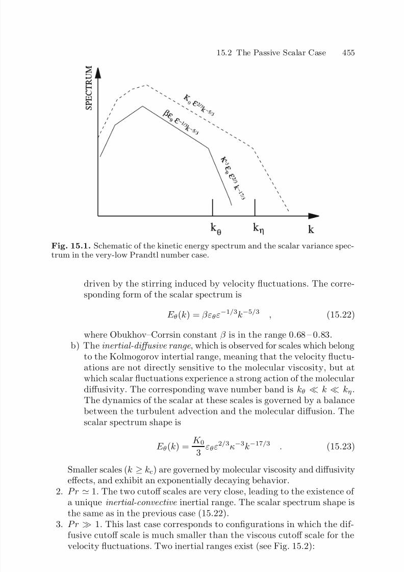
7/21/2019 Large Eddy Simulation for Incompressible Flows
http://slidepdf.com/reader/full/large-eddy-simulation-for-incompressible-flows 473/573
15.2 The Passive Scalar Case 455
Fig. 15.1. Schematic of the kinetic energy spectrum and the scalar variance spec-trum in the very-low Prandtl number case.
driven by the stirring induced by velocity fluctuations. The corre-sponding form of the scalar spectrum is
E θ(k) = βεθε−1/3k−5/3 , (15.22)
where Obukhov–Corrsin constant β is in the range 0.68 – 0.83.b) The inertial-diffusive range , which is observed for scales which belong
to the Kolmogorov intertial range, meaning that the velocity fluctu-ations are not directly sensitive to the molecular viscosity, but atwhich scalar fluctuations experience a strong action of the moleculardiffusivity. The corresponding wave number band is kθ k kη .
The dynamics of the scalar at these scales is governed by a balancebetween the turbulent advection and the molecular diffusion. Thescalar spectrum shape is
E θ(k) = K 0
3 εθε2/3κ−3k−17/3 . (15.23)
Smaller scales (k ≥ kc) are governed by molecular viscosity and diffusivityeffects, and exhibit an exponentially decaying behavior.
2. P r
1. The two cutoff scales are very close, leading to the existence of
a unique inertial-convective inertial range. The scalar spectrum shape isthe same as in the previous case (15.22).
3. P r 1. This last case corresponds to configurations in which the dif-fusive cutoff scale is much smaller than the viscous cutoff scale for thevelocity fluctuations. Two inertial ranges exist (see Fig. 15.2):

7/21/2019 Large Eddy Simulation for Incompressible Flows
http://slidepdf.com/reader/full/large-eddy-simulation-for-incompressible-flows 474/573
456 15. Coupling with Passive/Active Scalar
Fig. 15.2. Schematic of the kinetic energy spectrum and the scalar variance spec-trum in the very-high Prandtl number case.
a) An inertial-convective range , for wave numbers such that k kθ kB, which is similar to those already described above.
b) A viscous-convective range , which is associated to scales (kθ k kB ) where the velocity fluctuations are severely damped by viscouseffects but scalar fluctuations are not affected by molecular diffusion.The associated spectrum is
E θ(k) = 1
2
ν
εεθk−1 . (15.24)
This brief survey obviously shows that the spectral scalar transfers acrossthe large-eddy simulation cutoff may strongly depend on the type of inertial
range it is located in. As a consequence, the development of a closure basedon the functional modeling approach may be much more difficult than in theprevious case of the momentum equations, since the latter exhibits only onetype of inertial range dynamics.
Interscale Scalar Transfers. We now present some results dealing withthe analyis of passive scalar fluxes in the spectral space. These results arethe corner stone of the functional modeling approach. The emphasis is puton theoretical results coming from the EDQNM analysis of the passive scalardynamics in isotropic turbulence (see B.3 for a short presentation).
The main results of the EDQNM analysis deal with the non-local interac-tions in the scalar variance equation. Considering a non-local triad (k, p, q)satisfying the constraint k + p + q = 0, two cases are identified
– The considered scale, associated with k, is interacting with one much largerscale : p k q . The EDQNM form of the associated non-local scalar

7/21/2019 Large Eddy Simulation for Incompressible Flows
http://slidepdf.com/reader/full/large-eddy-simulation-for-incompressible-flows 475/573
15.2 The Passive Scalar Case 457
variance flux is
T θθ
+ (k) =
2
15 ak
0 Θθ
kkqq 2
E (q )dq 2kE θ(k) − k2 ∂E θ
∂k (k)+
1
4
ak0
Θθkkqq 3E θ(q )dqE (k)
− 1
4
ak0
Θθkkqq 5dq E (k)E θ(k)
k2 . (15.25)
The parameter a defines the local/non-local triads (see p. 93). The firstterm in the right hand side corresponds to interactions which are respon-
sible for the existence of the viscous-convective range.– The scale k is involved in a non-local triadic interaction with much smaller
scales: k p q . The asymptotic expression for the scalar variance fluxis
T θθ− (k) = −4
3
k0
q 2E θ(q )dq
+∞
sup(k,q/a)
ΘθqppE ( p)dp
+ 4
3 k
0
q 4dq +∞
sup(k,q/a)
ΘθqppE ( p)E θ( p)
p2
dp . (15.26)
A simplified expression, which is valid at low wave numbers, is
T θθ− (k) = −4
3k2E θ(k)
+∞
ak
Θθ0 ppE ( p)dp
+ 4
3k4
+∞
ak
Θθ0 ppE ( p)E θ( p)
p2 dp . (15.27)
The first term in the right hand side is associated with a forward scalar vari-ance cascade, whose intensity is governed by both the kinetic energy andscalar variance spectral distribution. The second term represents a back-ward scalar cascade.
The analysis of Direct Numerical Simulation results [783] reveals that,in the inertial-convective range, the overall spectral transfer is forward cas-cading. It is dominated by the energy-containing scales in the velocity field.More precisely, the dominant physical process at high wave numbers be-longing to this inertial range is a local transfer associated with a non-local
triadic interaction that links two high wave number scalar modes and one lowwave number velocity mode. The other non-local interactions (one high wavenumber scalar mode, one low wave number scalar mode and one high wavenumber velocity mode) and local interactions are much weaker. Therefore,the suggested dominant physical process is the breaking of “blobs” of scalarfluctuations into smaller-scale fragments by large energetic eddies.
7/21/2019 Large Eddy Simulation for Incompressible Flows
http://slidepdf.com/reader/full/large-eddy-simulation-for-incompressible-flows 476/573
458 15. Coupling with Passive/Active Scalar
The large-eddy simulation closure problem is now directly addressed bywriting the equation associated to the resolved scalar variance density, de-noted E θ(k) = G2(k)E θ(k):
∂
∂t + 2κk2
E θ(k) = T θθr (k) + T θθsgs(k) , (15.28)
where T θθr (k) and T θθsgs(k) are the resolved and the subgrid spectral scalarvariance transfer, respectively. In a way similar to the one used to characterizesubgrid kinetic energy transfers in Sect. 5.1.2, the intensity of these transfersacross a cutoff wave number kc can be parameterized defining an effectivespectral diffusivity κe(k|kc) such that
T θθsgs(k) = −2κe(k|kc)E θ(k) . (15.29)
In the case the cutoff is located within the inertial-conductive range, andassuming that all the basic hypotheses of the canonical analysis (inertialranges extending to infinity, sharp cutoff filter, see Sect. 5.1.2), both theEDQNM analysis conducted by Chollet and Zhou’s RNG theory [811] showthat the spectral effective diffusivity shape is strictly similar to the one of theeffective spectral viscosity ν e(k|kc):
– for k kc, it is independent of the wave number. The value of the plateaudeduced from the non-local forward cascade term in (15.27) is
κe(k|kc) = κ∞e ≡ 2
3
+∞
kc
Θθ0 ppE ( p)dp (15.30)
In practice, this plateau is observed for wave numbers in the range 0 ≤k ≤ kc/3. Theoretical analysis carried out by Chollet and Lesieur usingthe EDQNM analysis in the case of a very wide inertial-convective rangealso shows that the value of the plateau depends on both the kinetic energy
at the cutoff and the slope of the spectrum. A general expression is [514]:
κ∞e =
4
3a
√ 3 − m
m + 1
E (kc)
kcm < 3
1
3
1
m − 1
1√ Dr
E (kc)
kcm > 3
, (15.31)
where −m is the slope of the kinetic energy spectrum, a = 0.218K 0 a struc-
tural EDQNM parameter and Dr =
kc
0 k2E (k)dk a norm of the resolved
velocity gradient. Considering a Kolmogorov spectrum (m = 5/3, K 0 = 1.4)one obtains κ∞e = 0.3.– Near the cutoff, i.e. at wave numbers kc/3 ≤ k ≤ kc, the effective diffusivity
exhibits a cusp, showing that the spectral transfers are more intense. Inthis region, local interactions are not negligible. It is important notingthat this cusp is as sensitive as the one in the effective viscosity: it is

7/21/2019 Large Eddy Simulation for Incompressible Flows
http://slidepdf.com/reader/full/large-eddy-simulation-for-incompressible-flows 477/573
15.2 The Passive Scalar Case 459
not observed with smooth filters, and can also disappear if the cutoff islocated at the very beginning of the inertial range. In the canonical caseof an infinite inertial-convective range, the maximum value of the subgriddiffusivity found using EDQNM analysis is κe(kc|kc) = 0.6.
Detailed investigations of the spectral transfers across a cutoff locatedwithin the viscous-convective or the inertial-diffusive range are missing. Thislack in the theory may be not very important for most practical applications,since putting the cutoff within one of these inertial range requires the use of very fine computational grids.
Numerical experiments carried out by several authors [717] also show thatthe effective diffusivity spectral shape is very sensitive to both the scalar vari-
ance spectrum shape and the kinetic energy spectrum: it has been observedto be either an increasing or a decreasing function of the wave number. Effec-tive viscosities computed from simulated isotropic turbulence by Metais andLesieur are displayed in Figs. 15.3 and 15.4.
The Subgrid Prandtl Number Paradigm. The molecular Prandtl num-ber (15.18) is a useful tool to compare turbulent scales which characterizedissipative/diffusive cutoff scales of the velocity and scalar fields. This is whythe idea of introducing a subgrid Prandtl number , P rsgs, is attractive. Butpreceding remarks dealing with the sensitivity of the effective spectral diffu-
Fig. 15.3. Effective subgrid viscosity (Solid line ) and subgrid diffusivity (Dashed
line ) normalized by
E (kc)/kc in the Lesieur–Metais simulation (Case 1).
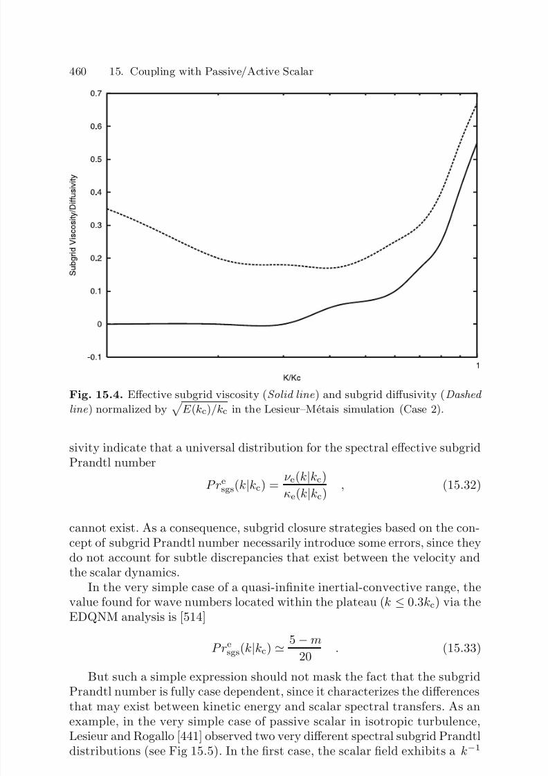
7/21/2019 Large Eddy Simulation for Incompressible Flows
http://slidepdf.com/reader/full/large-eddy-simulation-for-incompressible-flows 478/573
460 15. Coupling with Passive/Active Scalar
Fig. 15.4. Effective subgrid viscosity (Solid line ) and subgrid diffusivity (Dashed
line ) normalized by E (kc)/kc in the Lesieur–Metais simulation (Case 2).
sivity indicate that a universal distribution for the spectral effective subgridPrandtl number
P resgs(k|kc) =
ν e(k|kc)
κe(k|kc) , (15.32)
cannot exist. As a consequence, subgrid closure strategies based on the con-
cept of subgrid Prandtl number necessarily introduce some errors, since theydo not account for subtle discrepancies that exist between the velocity andthe scalar dynamics.
In the very simple case of a quasi-infinite inertial-convective range, thevalue found for wave numbers located within the plateau (k ≤ 0.3kc) via theEDQNM analysis is [514]
P resgs(k|kc) 5 − m
20 . (15.33)
But such a simple expression should not mask the fact that the subgridPrandtl number is fully case dependent, since it characterizes the differencesthat may exist between kinetic energy and scalar spectral transfers. As anexample, in the very simple case of passive scalar in isotropic turbulence,Lesieur and Rogallo [441] observed two very different spectral subgrid Prandtldistributions (see Fig 15.5). In the first case, the scalar field exhibits a k−1
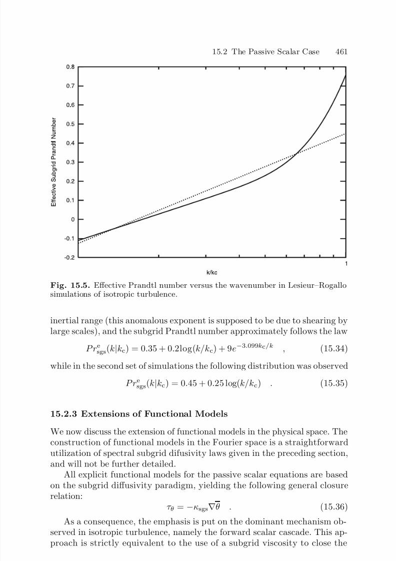
7/21/2019 Large Eddy Simulation for Incompressible Flows
http://slidepdf.com/reader/full/large-eddy-simulation-for-incompressible-flows 479/573
15.2 The Passive Scalar Case 461
Fig. 15.5. Effective Prandtl number versus the wavenumber in Lesieur–Rogallo
simulations of isotropic turbulence.
inertial range (this anomalous exponent is supposed to be due to shearing bylarge scales), and the subgrid Prandtl number approximately follows the law
P resgs(k|kc) = 0.35 + 0.2log(k/kc) + 9e−3.099kc/k , (15.34)
while in the second set of simulations the following distribution was observed
P resgs(k
|kc) = 0.45 + 0.25 log(k/kc) . (15.35)
15.2.3 Extensions of Functional Models
We now discuss the extension of functional models in the physical space. Theconstruction of functional models in the Fourier space is a straightforwardutilization of spectral subgrid difusivity laws given in the preceding section,and will not be further detailed.
All explicit functional models for the passive scalar equations are basedon the subgrid diffusivity paradigm, yielding the following general closurerelation:
τ θ = −κsgs∇θ . (15.36)
As a consequence, the emphasis is put on the dominant mechanism ob-served in isotropic turbulence, namely the forward scalar cascade. This ap-proach is strictly equivalent to the use of a subgrid viscosity to close the

7/21/2019 Large Eddy Simulation for Incompressible Flows
http://slidepdf.com/reader/full/large-eddy-simulation-for-incompressible-flows 480/573
462 15. Coupling with Passive/Active Scalar
filtered momentum equations. Almost all functional subgrid models and/orclosure strategies proposed for the momentum equations and presented inChaps. 5 and 6 can be very easily extended to the scalar equation. An ex-haustive description of all possibilities is not of interest, and it is worth not-ing that many straightforward extensions have not been published yet3. Theimplicit Large-Eddy Simulation approach can also be used, if an adequatenumerical scheme for the scalar equation is utilized.
General Expression. Scalar Subgrid Diffusivity. As in the case of sub-grid viscosity, a fully general expression of the subgrid diffusivity κsgs asa function of a set of selected basic quantities can be used to obtain a unifiedview of most published models. A possible expression is
κsgs = κsgs(Pr,∆, |S |, q 2sgs, ε, |∇θ|, θ2sgs, εθ) , (15.37)
where quantities directly tied to subgrid quantities (i.e. q 2sgs, ε , θ2sgs, εθ) can
be evaluated solving corresponding prognostic equations, or using some localequilibrium and/or scale similarity assumptions to recover expressions involv-ing resolved scales only. The Prandtl number is a priori included as an inputof this general expression, since it can be used to distinguish the different iner-tial range regimes. Weighting coefficients in the constitutive equation (15.37)
are found performing a simple dimensional analysis.An example is the model proposed by Schmidt and Schumann [651]:
κsgs = C κ∆
q 2sgs , (15.38)
where interial-conductive range considerations lead to
C κ =
2
3K 0
1
3βπ . (15.39)
Yoshizawa [789] proposes a more complex model:
κsgs = C (θ2
sgs)2ε
ε2θ
, C = 0.446 . (15.40)
A subgrid diffusivity model which accounts for molecular Prandtl numbereffects was developed by Grotzbach [277, 279] to describe the temperaturefield in liquid metals, which have very small Prandtl number (P r = 0.007for liquid sodium under nuclear reactor conditions). We reproduce here the
method developed by Grotzbach to account for small Prandtl number effectsrather than its model, since it can be applied to any subgrid viscosity modelwith one arbitrary constant. Let us consider a generic subgrid diffusivity
3 The interested reader will quickly find material for a few dozens of papers dealingwith “new improved models”!

7/21/2019 Large Eddy Simulation for Incompressible Flows
http://slidepdf.com/reader/full/large-eddy-simulation-for-incompressible-flows 481/573
15.2 The Passive Scalar Case 463
model under the formκsgs = C K , (15.41)
where C is the constant to be adjusted and K a constant-free parameterwhich has the dimension of a diffusivity. The method proposed by Grotzbachrelies on the local equilibrium assumption (i.e. production = dissipation) forthe scalar variance:
τ θ · ∇θ = εθ − κ∇θ · ∇θ , (15.42)
where εθ is the full turbulent scalar variance dissipation. Now introducing themodel in the left hand side of this relation, one obtains the following relationfor the constant C :
C =
εθ
−κ
∇θ
· ∇θ
−K∇θ · ∇θ . (15.43)
The last parameter to be evaluated is εθ. Assuming that the cutoff occursin a very wide inertial-convective range, an analytic expression for the scalarvariance dissipation as a function of the kinetic energy dissipation can befound, yielding
C 1
β √
K 0
1 − βκε−1/3∆
−4/3
, (15.44)
where the subgrid kinetic energy dissipation rate ε is retrieved from the workdone to close the momentum equation, leading to a fully determined definitionof the subgrid diffusivity.
The Subgrid Prandtl Number Approach. A very common closure ap-proach is to use a subgrid Prandtl number, leading to
κsgs = ν sgs
P rsgs, (15.45)
where the subgrid viscosity ν sgs can be evaluated using any model described inthe preceding chapters devoted to the momentum equation closure. Despite it
is flawed from a purely theoretical point of view, this approach is very oftenused in simulations in the physical space and the subgrid Prandtl numberappears as an adjustable parameter which can be tuned in an ad hoc way toobtain the best fit with the reference data. Values found in the literature rangefrom 0.1 to 1, the most common one being 0.6. It is important noting thatthis approach is not valid in cases where the velocity field if fully resolved,yielding ν sgs = 0, while some subgrid scalar fluctuations exist. A typicalexample would be to put the resolution cutoff within the viscous-convectiverange.
The subgrid Prandtl number can be made more accurate, but still notadequate to represent the cases mentioned above, rendering it self-adaptive,meaning that the value of the Prandtl number will be made space and timedependent. Such a modification is expected to make the subgrid Prandtlnumber based models adequate to treat the case where all scalar fluctua-tions are resolved while subgrid kinetic energy transfers exist. A common

7/21/2019 Large Eddy Simulation for Incompressible Flows
http://slidepdf.com/reader/full/large-eddy-simulation-for-incompressible-flows 482/573
464 15. Coupling with Passive/Active Scalar
example is to use the Germano identity to define a dynamic procedure, asproposed by Moin et al. [538]. The Germano identity for the scalar equationis uθ − uθ
Lθ
= uθ − uθ T θ
− uθ − uθ τ θ, (15.46)
where the tilde symbol refers to the test filter level. Vectors T θ and τ θ are thesubgrid scalar fluxes at the grid and test filter levels, respectively. As in theanalogous relation for the momentum equation, the left hand side of (15.46)can be directly computed, while replacing subgrid fluxes in the right handside by the corresponding subgrid models makes it possible the find the bestvalue of the model constant in the least-square sense.
Denoting ν sgs(∆) and ν sgs(∆) the subgrid viscosity values computed at thegrid and test filter levels, respectively, the residual associated to the Germanoidentity (15.46) is equal to
E θ = Lθ + ν sgs(∆)
P rsgs∇θ −
ν sgs(∆)
P rsgs∇θ . (15.47)
Assuming that the subgrid Prandtl number is the same at the two levels
and that it does not vay significantly over distances of the order of ∆, the
least-square minimization of E θ leads to
P rsgs = −mθ · mθ
mθ · Lθ, (15.48)
where
mθ ≡ ν sgs(∆)∇θ − ν sgs(∆)∇θ . (15.49)
Other expressions can be derived. As an example, Moin et al. [538] do notuse the least-square minimization but chose to find the value of P rsgs which
corresponds to a zero of E θ
· ∇θ:
P rsgs = −mθ · ∇θ∇θ · Lθ
. (15.50)
Wong and Lilly [766] define a dynamic procedure based on dimensionalparameters, yielding
P rsgs = (L :
S )
|S
|2
(Lθ · ∇
θ)
∇θ · ∇θ. (15.51)
All these dynamic subgrid Prandtl number definitions suffer some numer-ical stability problems. The methods used to cure this problem are the sameas for the momentum equation (see Sect. 5.3.3 ): clipping, time/space averag-ing, ... All variants of the dynamic procedure described in preceding chapterscan be applied to compute the dynamic subgrid Prandtl number.
7/21/2019 Large Eddy Simulation for Incompressible Flows
http://slidepdf.com/reader/full/large-eddy-simulation-for-incompressible-flows 483/573
15.2 The Passive Scalar Case 465
Anisotropic Subgrid Diffusivity. All models mentioned above are basedon inertial range considerations, which are characteristic features of homoge-neous isotropic turbulence. Practical applications involve much more complexconfigurations, in which the scalar field can be non homogeneous while thevelocity field remains isotropic, or even more complex flows were both thevelocity and the scalar fields are not homogeneous. Therefore, the questionarises of accounting for the velocity field anisotropy in the scalar diffusion.This task is expected to be much more complex than the equivalent one forthe velocity field, since the scalar variance spectrum exhibits much less uni-versal features than the kinetic energy spectrum. Experiments conducted byKang et al. [376] also show that the trend of decreasing anisotropy at smallscales observed on velocity fluctuations is not recovered on scalar fluctuations.
It is also known that, in the presence of a mean scalar gradient, structurefunctions and the derivative skewness of the scalar field do not follow predic-tions from isotropy at inertial and even dissipative scales. This local isotropybreakdown is tied to the direct action of large velocity structures on smallscalar scales (this is consistent with the EDQNM analyis results dealing withdominant triadic interactions).
Taking anisotropy into account can be an important issue when the cutoff is such that the subgrid scalar fluctuations are governed by velocity fluctua-tions with high local Reynolds number (the localness is understood here in
terms of wave number). In such cases, anisotropy in the velocity field will havean effect on the scalar diffusion process, and the most simple idea consists indefining a tensorial subgrid diffusivity.
Yoshizawa [789] proposes the following anisotropic diffusivity, which isderived using a two-scale expansion:
(κsgs)ij = −C
θ2
sgs
εθ
3
εS ij , (15.52)
where C = 0.366. The subgrid scalar dissipation rate and the subgrid scalarvariance remain to be evaluated. Models for these quantities are presented inSect. 15.2.6. The use of the resolved strain tensor S is coherent with the simplephysical picture that scalar “blobs” are stretched by the velocity fluctuations,and will therefore be elongated in the principal shear direction, leading tothe development of smaller scalar scales in transverse directions. A similarmodel is proposed by Peng and Davidson [587]. Rotational effects can alsobe included by taking into account the skewsymmetric part of the resolvedvelocity gradient, Ω ij :
(κsgs)ij = −2ε
θ2
sgs
εθ
3 C 1S ij + C 2Ω ij
, (15.53)
with C 1 = 0.29 and C 2 = 0.08.

7/21/2019 Large Eddy Simulation for Incompressible Flows
http://slidepdf.com/reader/full/large-eddy-simulation-for-incompressible-flows 484/573
466 15. Coupling with Passive/Active Scalar
Another tensorial subgrid diffusivity model was proposed by Pullin [608],who extended the stretched-vortex approach (see Sect. 7.6) to the passivescalar case. In the extended model, it is assumed that the subgrid mixingis restricted to the plane normal to the vortex axis. A secondary propertyof this model is that the subgrid scalar gradient induced by the transportis orthogonal to the subgrid vorticity, the latter being represented by thestretched vortex. This is consistent with the observations that the probabilitydensity of the alignement between the vorticity and the scalar gradient ismaximum when these vectors are orthogonal. The corresponding formulationis
(κsgs)ij = γπ
2kc q 2sgs
δ ij − evi evj
, (15.54)
where the vector ev is the same as in Sect. 7.6. Assuming that the cutoff occurs within an infinite inertial-convective range, the structural parameter γ is given by
γ = 2
π
2
3K 0
1
β . (15.55)
15.2.4 Extensions of Structural Models
Many structural models have been applied to the subgrid scalar flux vector.
The most illustrative ones are presented below.
Approximate Deconvolution and Scale Similarity Models. Scale sim-ilarity, or, in an equivalent way, soft approximate deconvolution models aredefined writing the following approximation:
τ θ ≡ uθ − uθ ≈ u•θ• − uθ , (15.56)
where the approximate defiltered fields are expressed as
u• = G−1l u, θ• = G−1l θ , (15.57)
with G−1l an approximate inverse of the filter (see Sect. 7.2.1 for a detailed
presentation). A large number of structural models can be generated usingthis simple form, as for the momentum equation: models based on iterativedeconvolution, models based on Taylor series expansions and tensor diffusiv-ity models. Because they are all approximations of the exact soft deconvolu-tion solution, these models do not take into account scalar transfer towardssubgrid scales and they must be supplemented with a dissipative term, which
can be either a numerical regularization or a functional subgrid model. Thatleads to the definition of linear combination models for the subgrid scalarfluxes.
The Bardina-type model obtained using the lowest-order deconvolution is
τ θ = uθ − uθ . (15.58)
7/21/2019 Large Eddy Simulation for Incompressible Flows
http://slidepdf.com/reader/full/large-eddy-simulation-for-incompressible-flows 485/573
15.2 The Passive Scalar Case 467
The associated gradient-type model is (for a Gaussian or Box filter)
τ θ = ∆
2
24 ∇2(uθ) . (15.59)
Differential Scalar Fluxes Model. Another solution consists in solvinga differential equation for each component of the subgrid scalar flux vector.This approach requires to close (15.7), in which terms V (pressure-scalarcorrelations) and V I (diffusion by subgrid fluctuations) are not directly com-putable.
Deardorff [173] proposes to close term V as
τ G
θ,
∂p
∂xi
= −C 1
q 2sgs
∆τ G(ui, θ) , (15.60)
and to express the third-order term as
τ G(uk, ui, θ) = −C 2∆
q 2sgs
∂
∂xiτ G(uk, θ) +
∂
∂xkτ G(ui, θ)
, (15.61)
with C 1 = 4.8 and C 2 = 0.2.Other closures are derived by Sheikhi et al. [671], who use the velocity-
scalar filtered density function approach. This method is strictly equivalentto the one developed by Gicquel et al. for the momentum equation (seeSect. 7.5.3): a stochastic field whose probability density function is the so-lution of the evolution equation of the filtered density probability functionis computed via a Lagrangian-Monte-Carlo method. In the present case, themethod is utilized to reconstruct both u and θ. These reconstructed stochas-tic variables can be used to close the filtered momentum and scalar equations
directly, or to close the equations for the subgrid scalar fluxes and the sub-grid scalar variance. The latter approach is considered here, since the formerbelongs to the family of the methods based on a direct evaluation of the sub-grid scales (to be discussed below). This approach yields the following closurerelation for the sum of the pressure-scalar correlations and the dissipation:
2ντ G
∂ui∂xk
, ∂θ
∂xk
+ τ G
θ,
∂p
∂xi
= ω
3
2 +
3
4C 0
τ G(ui, θ) , (15.62)
where C 0 = 2.1 and the time scale ω is equal to
ω =
q 2sgs
∆. (15.63)
The triple correlation term is directly computed using the stochastic sub-grid field.
7/21/2019 Large Eddy Simulation for Incompressible Flows
http://slidepdf.com/reader/full/large-eddy-simulation-for-incompressible-flows 486/573
468 15. Coupling with Passive/Active Scalar
Explicit Evaluation of Subgrid Scales, Multilevel Simulations andOthers. The technique consisting in regenerating the subgrid scales of thescalar field on a finer mesh using a low-cost stochastic model, a simplifieddeterminitic model or multilevel simulation has also been extended to thepassive scalar case. These extensions being very reminiscent of their counter-parts for the momentum equation, they will not be detailed here.
15.2.5 Generalized Subgrid Modeling for Arbitrary Non-linearFunctions of an Advected Scalar
The preceding sections addressed the problem of finding subgrid closuresfor the convection term, the other ones being assumed to be linear. But inmany flows, additional physical processes associated to scalar source/sink arepresent, which appear as non-linear functions of the scalar field θ. Commonexamples are chemical reactions, fluids with temperature-dependent molecu-lar viscosity/diffusivity, or coupling of the scalar field (density, temperature,concentration) with micro-physics such as radiative transfer. Let us considera general form for this additional source term:
∂θ
∂t + ∇ · (uθ) = κ∇2θ + f (θ)
source term
. (15.64)
The corresponding source term in the filtered scalar equation is f (θ),which is decomposed as
f (θ) = f (θ) computable
+
f (θ) − f (θ)
τ f :subgrid term
. (15.65)
The new closure problem consists in finding a surrogate for τ f . Since we
are addressing a fully general problem which can cover a very wide rangea physical mechanisms, the definition of a general functional model is hope-less. Specific functional models can be found for individual process, as it isdone for the convection term.
The most general approach being the structural modeling, Pantano andSarkar [578] propose to use an approximate deconvolution approach to modelgeneral subgrid source terms (in practice, they applied this strategy toa chemical reaction term) . The key idea developed by these authors is to ap-proximate θ by a synthetic field θ• which is optimized so that it will minimize
an error functional, leading to
f (θ) − f (θ) = f (θ•) − f (θ•) . (15.66)
Since physical processes may be very sensitive to small errors and are as-sociated to high-order non-linearities in terms of θ (e.g. the radiative transfer

7/21/2019 Large Eddy Simulation for Incompressible Flows
http://slidepdf.com/reader/full/large-eddy-simulation-for-incompressible-flows 487/573
15.2 The Passive Scalar Case 469
flux behaves as θ4, where θ is the temperature), it is important to enforcesome accuracy requirements when defining θ•.
The simple Taylor series expansion
f (θ) − f (θ) = 1
2f (θ)(θ2 − θ
2) + ... , (15.67)
illustrates the fact that a good control of the error committed on the subgridscalar variance is necessary to ensure a satisfactory representation of thesubgrid source/sink term. As a consequence, Pantano and Sarkar propose tomodify the usual soft deconvolution procedure, leading to
θ•
= θ + C 0(θ − θ) + C 1(θ − 2θ + θ) + ... , (15.68)
were the coefficients C i are allowed to vary, instead of being fixed to beunity as in the original approximate deconvolution procedure based on theVan Cittert iterative method (7.8). These coefficients are chosen in order tomake the statistical mean filtered moments that appear in the Taylor se-ries expansion of the modeled field equal to their counterparts defined usingthe exact field. In practice, it is aimed to enforce the following global con-straints
Ω
θ•k − θ•k
dx = Ω
θk − θk
dx, k = 2, ..., N , (15.69)
where N is an arbitrary parameter and Ω is the fluid domain under consider-ation. Practical subgrid models are derived truncating expansion (15.68) atan arbitrary order and inserting it in (15.69). To get a closed set of non-linearpolynomial equations for the coefficients C i, it is also required to select ananalytic expression of the scalar spectrum and the filter transfer function.
15.2.6 Models for Subgrid Scalar Variance and Scalar SubgridMixing Rate
This section is devoted to models aiming at evaluating the two following sub-grid quantities, which characterize the dynamics of the subgrid fluctuationsof the scalar field θ:
– The subgrid scalar variance, θ2sgs, also referred to as the scalar unmixedness ,
since it measures the degree of local non homogeneity of θ within thevolume of characteristic diameter ∆: a uniform distribution is associated
with a zero subgrid variance.– The scalar variance dissipation rate, εθ, also referred to as the scalar vari-
ance destruction rate, which is related to the stirring and mixing processat subgrid scales. A high destruction rate means that diffusion is quicklyhomogenezing the scalar field.

7/21/2019 Large Eddy Simulation for Incompressible Flows
http://slidepdf.com/reader/full/large-eddy-simulation-for-incompressible-flows 488/573
470 15. Coupling with Passive/Active Scalar
A large number of subgrid models for these two quantities have beenproposed, since they are important inputs of subgrid models for combustionrelated terms. Since the specific problem of reactive flows is beyond the scopeof this chapter, this section illustrates the different modeling ways and doesnot provide the reader with an exhaustive description.
Models for the Subgrid Scalar Variance. It is worth noting that theissue of predicting θ2
sgs is reminiscent of the one dealing with the evaluationof the subgrid kinetic energy, q 2sgs. Therefore, all methods and models definedto compute the latter (see Sect. 9.2.3) can be modified to evaluate the former.This work is straightforward and is left to the interested reader. Only generalapproaches will be discussed in this section.
The subgrid scalar variance being defined as
θ2sgs ≡ θ2 − θ
2, (15.70)
a natural way to model it is to use a deconvolution-type approach (or itsoptimized version proposed by Pantano and Sarkar for arbitrary non-linearfunctions of θ, see Sect. 15.2.5). The usual deconvolution procedure yields
θ2sgs θ•2 − θ•
2, (15.71)
where θ• = G−1l θ is the approximate defiltered field. Using the zeroth-order
expansion of the deconvolution operator, one obtains a scale-similarity typemodel:
θ2sgs C (θ
2 − θ2
) , (15.72)
where the constant C is equal to one if the Van Cittert method is used.Other values can be found using a dynamic procedure based on a Germano-type identity. A gradient type model is recovered replacing the convolutionfilters by their equivalent differential expansion, and then truncating these
expansion at an arbitrary order. For box and Gaussian filters, the first orderterm is
θ2sgs C ∆
2|∇θ|2 , (15.73)
where the parameter C is filter dependent and can be adjusted using a dy-namic procedure.
The subgrid scalar variance can also be easily retrieved if a structuralmodel based on an explicit reconstruction of the subgrid scales is used toclose the filtered scalar equation. In this case, it is directly computed fromthe synthetic subgrid scalar field. It is also straightforwardly extracted if a differential model for the scalar fluxes is used.
Another possiblity consists in solving a prognostic equation for θ2sgs, in
a way similar to what is done for the subgrid kinetic energy. Using (15.8)as a starting point, a closed equation is obtained. The resulting model is
7/21/2019 Large Eddy Simulation for Incompressible Flows
http://slidepdf.com/reader/full/large-eddy-simulation-for-incompressible-flows 489/573
15.2 The Passive Scalar Case 471
presented in (15.135) for the sake of brevity. Prognostic equations with dy-namic coefficients can also be derived using techniques presented in Sect. 5.4(p. 173) for the transport equation of the subgrid kinetic energy.
A simple expression is obtained in the simplified case where the inertial-convective range spectrum (15.22) is assumed to be valid at all subgrid wavenumbers:
θ2sgs =
+∞
π/∆
E θ(k)dk = 3β
2π2/3εθε−1/3∆
2/3. (15.74)
Models for the Subgrid Scalar Dissipation Rate. A first simple evalu-ation of εθ is obtained assuming that the cutoff is located within an infiniteinertial-convective range:
εθ = C θ2
sgs q 2sgs
∆, (15.75)
where the constant C can by either computed analytically or adjusted usinga dynamic procedure. Considering an infinite inertial-convective range, oneobtains
C = 2π
3β
2
3K 0. (15.76)
The other way to evaluate the subgrid scalar variance dissipation rate is
to assume that the local equilibrium hypothesis holds: in this case, it is equalto the local subgrid scalar variance production rate, leading to
εθ = −τ θ · ∇θ , (15.77)
where the subgrid scalar flux τ θ can be evaluated using any adequate subgridmodel. If a subgrid diffusity model is utilized, one obtains
εθ = 2κsgs|∇θ|2 . (15.78)
This expression can be modified to account for the dissipation at theresolved scales, yielding
εθ = 2(κ + κsgs)|∇θ|2 . (15.79)
In order to obtain a more general expression which does not rely on thelocal equilibrium assumption, Jimenez et al. [352] assumed that the charac-teristic subgrid mixing time is proportional to the subgrid turbulent time:
εθθ2
sgs
∝ ε
q 2sgs
, (15.80)
yielding the following model
εθ = C θ2
sgsε
q 2sgs
, (15.81)

7/21/2019 Large Eddy Simulation for Incompressible Flows
http://slidepdf.com/reader/full/large-eddy-simulation-for-incompressible-flows 490/573
472 15. Coupling with Passive/Active Scalar
where C is a parameter. Tests show that C = 1/P r leads to satisfactoryresults. All quantities which appear in the right hand side of (15.81) can beevaluated using ad hoc models.
15.2.7 A Few Applications
– Heat transfer at free surface [93]– Heat transfer in plane channel flow [92, 755, 196, 753]– Isotropic turbulence [121, 441, 538, 122, 220, 608, 344, 345, 752]– Complex cavities and ducts [279, 590, 639]– Homogeneous turbulence [344, 345]– Time-developing shear layer [344, 345]– Flow past a backward facing step [27]– Jet impinging on a plate [738, 155, 126, 236]– Flow in a corrugated passage [141]– Mixing Layer [168]– Flow in rotating/steady duct with/without rib [557, 558, 559, 560]– Flow in S-shaped duct [561]– Wall-mounted cube matrix [565]
15.3 The Active Scalar Case:Stratification and Buoyancy Effects
We now turn to the case of the coupling with an active scalar, i.e. witha field which has a feedback effect on the velocity field, leading to a two-waycoupling between the Navier–Stokes and the scalar equations. Since there area very huge number of possible interactions, it is chosen to put the emphasison buoyancy and stable stratification effects. Other physical models, such as
Eulerian–Eulerian models for two-phase flows, will not be considered.
15.3.1 Physical Model
Buoyancy and stable stratification effects originate in the force to whicha blob of fluid is submitted when it is immersed in a fluid with differentdensity. Therefore, a natural physical parameter to describe these effects isthe density. When very weak compressiblity effects are taken into account,the density of “usual” fluids is assumed to decrease when the temperature is
increased. Thus, the temperature can also be used to represent the dynamicsof these flows. Both solutions are found in the literature, depending on theauthors and specific purposes of the studies. In the following, the scalar fieldθ will be related to the temperature field.
Using the Boussinesq approximation (see reference books for a detaileddiscussion of the range of validity of this model, e.g. [714, 708, 439]), the

7/21/2019 Large Eddy Simulation for Incompressible Flows
http://slidepdf.com/reader/full/large-eddy-simulation-for-incompressible-flows 491/573
15.3 The Active Scalar Case: Stratification and Buoyancy Effects 473
basic set of unfiltered equations consists in the Navier–Stokes equationswith a gravitational source term supplemented by a scalar equation iden-tical to (15.1):
∂ u
∂t + ∇(u ⊗ u) = −∇ p + ν ∇2u +
θ − Θ
Θ0g
feedback term
, (15.82)
∇ · u = 0 , (15.83)
∂θ
∂t + ∇ · (uθ) = κ∇2θ , (15.84)
where θ is potential temperature , defined as the thermodynamic temperature
increased by the normalized gravitational potential, g
= (0, 0, −g) the gravityvector and Θ is the potential temperature field associated to the hydrostaticequilibrium. The vector g is related to the gravitational acceleration. Θ0 isrelated to a reference value, which is assumed to be unique for the whole flowdomain. The molecular viscosity and the molecular diffusivity are assumedto be constant and uniform.
The corresponding set of filetered equations is very similar to those usedin previous chapters, since the original set of equations differs by only onesource term:
∂ u∂t
+ ∇(u ⊗ u + τ ) = −∇ p + ν ∇2u + θ − ΘΘ0
g , (15.85)
∇ · u = 0 , (15.86)
∂θ
∂t + ∇ · (uθ + τ θ) = κ∇2θ , (15.87)
where it has been assumed that the scale separation operator perfectly com-mutes with all partial derivatives operator and that the mean field Θ isvarying slowly enough in space to have Θ = Θ. The subgrid fluxes τ and τ θhave exactly the same expressions as in the passive scalar case.
A deeper insight into the two-way coupling is gained rewriting the evolu-tion equations for the subgrid quantities. Assuming that the vertical directionis associated to x3, the equations for the subgrid mometum fluxes are:
∂τ G(ui, uj)
∂t + uk
∂τ G(ui, uj)
∂xk= −τ G(uk, ui)
∂uj∂xk
− τ G(uk, uj)∂ui∂xk
+ν ∂ 2τ G(ui, uj)
∂xk∂xk− 2ντ G
∂ui∂xk
, ∂ uj∂xk
−τ Guj,
∂p
∂xi− ∂τ G(uk, ui, uj)
∂xk
+ g
Θ0(δ i3τ G(uj , θ) + δ j3τ G(ui, θ))
coupling term
,
(15.88)
7/21/2019 Large Eddy Simulation for Incompressible Flows
http://slidepdf.com/reader/full/large-eddy-simulation-for-incompressible-flows 492/573
474 15. Coupling with Passive/Active Scalar
and the corresponding equations for the generalized subgrid kinetic energyis:
∂τ G(ui, ui)∂t
= ∂ ∂xj
12
τ G(ui, ui, uj) + τ G( p, uj) − ν ∂τ G(ui, ui)∂xj
− ντ G
∂ui∂xj
, ∂ui∂xj
− τ G(ui, uj)
∂ui∂xj
+ δ i3g
Θ0τ G(θ, ui)
coupling term
. (15.89)
The subgrid scalar fluxes are solutions of
∂τ G(ui, θ)
∂t + uk
∂τ G(ui, θ)
∂xk= −τ G(uk, ui)
∂θ
∂xk− τ G(uk, θ)
∂ui∂xk
+ ∂
∂xk
ντ G
∂ui∂xk
, θ
+ κτ G
∂θ
∂xk, ui
−(ν + κ)τ G
∂ui∂xk
, ∂θ
∂xk
− τ G
θ,
∂p
∂xi
−∂τ G(uk, ui, θ)
∂xk
+ δ i3g
Θ0
τ G(θ, θ) coupling term
, (15.90)
while the generalized subgrid scalar variance equation is kept unchanged,since there is no gravitational source term in the scalar equation. Therefore,the subgrid variance is not directly affected by the feedback effect on thevelocity field, but it is sensitive to it via changes in the latter.
15.3.2 Some Insights into the Active Scalar Dynamics
Flows governed by (15.82)–(15.84) exhibit a very wide and complex rangeof physical mechanisms, which originate in the coupling that may exists be-tween convection, diffusion, stratification and other features such as meanshear, rotation and boundary conditions. It is meaningless to try to give anexhaustive description of all these possibilities. The present section will focuson very simple cases and the emphasis will be put on results dealing withinterscale transfers, which are of primary interest for subgrid modeling.
The influence of the stratification effects on the subgrid kinetic energy isseen looking at the last term of (15.89), which can lead to an increase asso-
ciated to buoyancy effect or a decrease due to stable stratification damping,depending on its sign. Its relative importance with respect to the productionterm is measured by the flux Richardson number:
Rif =
gΘ0
τ G(u3, θ)
τ G(ui, uk) ∂ui∂xk
, (15.91)

7/21/2019 Large Eddy Simulation for Incompressible Flows
http://slidepdf.com/reader/full/large-eddy-simulation-for-incompressible-flows 493/573
15.3 The Active Scalar Case: Stratification and Buoyancy Effects 475
High values of Rif are associated to flows in which stratification effects aredominant, while they can be neglected when Rif 1. Neglecting energytransport across the flow, one obtains
Rif 1 − ε
−τ G(ui, uk) ∂ui∂xk
, (15.92)
showing that destabilizing effects are present if Rif > 1 (the denominator of the last term being assumed to be positive).
Two basic cases are discussed in the present section:
– The case of stable stratification (p. 475), in which stratification effects tendto damp the subgrid kinetic energy. An important feature of flows withstable stratification is the existence of dispersive internal gravity waves.These waves are important in many applications dealing with meteorologyand oceanology. They induce irrotational large-scale horizontal motions,whose interactions with small scale turbulence will be one of the mostimportant issue discussed below.
– The case of unstable stratification (p. 480), where buoyancy effects generateturbulence, a well known example being thermal plumes.
Another relevant parameter is the group
N = g
Θ0
∂θ
∂z . (15.93)
Under the assumption that the subgrid heat flux τ G(θ, u) obeys a Fickian-like law, i.e. τ G(θ, u) −C ∇θ, where C is a positive constant, it is seenfrom (15.88), (15.89) and (15.90) that the local stablizing/destabilizing effectof stratification depends on the sign of N , i.e. on the local sign of the verticalresolved gradient ∂θ/∂z:
1. If ∂θ/∂z > 0, the effect is stabilizing, since it appears as a sink term in thesubgrid kinetic energy equation. In this regime, gravity waves are stableand their frequency is characterized by the Brunt–Vaisala frequency, N ≡√ N .
2. If ∂θ/∂z < 0, gravity waves are unstable and break up into turbulence:the buoyancy effects are seen to increase the production of subgrid kineticenergy. The buoyancy time scale is estimated as T b ≡ 1/
√ −N .
Energy Transfers in Stably Stratified Flows. Energy transfers in sta-
bly stratified flows have been addressed by many authors, and are observedto be case dependent. Therefore, no general description of the transfer acrossa cutoff similar to what exists for the momentum equation is available, themain explanation for that being that such a general description is nearlyimpossible. The difficult points which preclude such an analysis are the fol-lowing

7/21/2019 Large Eddy Simulation for Incompressible Flows
http://slidepdf.com/reader/full/large-eddy-simulation-for-incompressible-flows 494/573
476 15. Coupling with Passive/Active Scalar
– These flows are strongly anisotropic, and it has already been seen thatkinetic energy transfers within homogeneous anisotropic flows cannot bedescribed in a simple and general way, since they are case-dependent.
– The description in terms of interscale transfers is not sufficient to obtainan accurate picture of the governing physical processes. It appears thatthe concept of modes must be introduced to achieve a meaningful analysis:the energy must be split into the vortex kinetic energy and the total wave energy , the latter being further decomposed into the potential energy andthe wave kinetic energy [266]. The analysis of triadic interactions using thisscheme leads to a global description which is too complex to yield resultsthat can be straightforwardly utilized for subgrid parameterization. Thismodal decomposition results from a local decomposition of the velocity and
temperature field in the Fourier space:
u(k) = u1(k) + u2(k) , (15.94)
where u1(k) and u2(k) are related to the vortex and internal gravity wavecomponents, respectively, with
u1(k) =
φ1(k)e1(k),
u2(k) =
φ2(k)e2(k) , (15.95)
where
e1(k) = k × g|k × g| , e2(k) = k × e1(k)
|k × e1(k)| . (15.96)
The two vectors (e1(k), e2(k)) generate an orthonormal basis for the planeperpendicular to k. The vortex kinetic energy spectrum, Φ1(k), the wavekinetic energy spectrum, Φ2(k), and the potential energy spectrum P (k)are defined as follows:
Φ1(k) = 1
2 φ1(k)
φ1(−k)
, Φ2(k) =
1
2 φ2(k)
φ2(−k)
,
P (k)(k) = 1
2N 2 θ(k) θ(−k)
,
where N 2 is equal to the square of the Brunt-Vaisala frequency built onthe mean temperature gradient:
N 2 = g
Θ0
dΘ
dz . (15.97)
The total kinetic energy spectrum is recovered summing the vortex and
wave contributions: E (k) = Φ1(k) + Φ2(k).
As a consequence, this section will be devoted to the description of themain features of very simple cases which have been very accurately analyzedusing both theoretical tools and direct numerical simulation.
7/21/2019 Large Eddy Simulation for Incompressible Flows
http://slidepdf.com/reader/full/large-eddy-simulation-for-incompressible-flows 495/573
15.3 The Active Scalar Case: Stratification and Buoyancy Effects 477
The most simple case is initially isotropic turbulence submitted thestrong stabilizing effects. The main observed phenomenon is the break-down of isotropy, associated to a drastic restriction of motion along themean stratification direction. After some times, the flow is organized in thinlayers with a strong variability along the stratification direction (pancake-shaped large-scale vortices), leading to the occurance of a velocity field whichis almost two-component 4 Detailed investigations of energy transfers usingDirect Numerical Simulation and EDQNM models have been carried out[235, 304, 513, 266, 689, 267]. The main results are the following
– Several phases are observed, the number of which being dependent on theinital condition and the value of the Richardson number. The first phase (if
initial potential energy is large enough) corresponds to a flow whose largescales are governed by stratification effects and inertial gravity waves andexhibit a N 2k−3 kinetic energy spectrum, while small scales are not affectedby stratification effects and are governed by the usual isotropic turbulentdynamics. In the last phase, all scales are anisotropic and stratificationeffects drive the whole flow.
– During the first phase (pre-collapse phase), the flow dynamics is controlledby the potential energy being transferred from large to small scales ata higher rate than kinetic energy, leading to a higher total energy decay as
in unstratified isotropic turbulence. The kinetic energy along the stratifi-cation direction is converted into potential energy, feeding the irreversibleforward cascade of potential energy. A consequence of the potential energycascade is the existence of a persisting counter-gradient scalar flux. Sucha counter-gradient scalar flux should be associated to a negative subgriddiffusivity at small scales, making all previous models irrelevant. But thiscounter-gradient flux seems to play no major dynamical role on the smallestscales during the first phase if the molecular diffusivity is high enough.
– The final phase (post-collapse phase) is associated to a scalar flux collapseat large scales. The ratio of the kinetic energy along the the stratificationdirection and the potential energy reach a constant value, while large-scaleenergetic motion in directions perpendicular to the mean stratification di-rection arise from turbulence, forming the vortex part of the flow. Thesmall scale dynamics is dominated by stratification effects. An explana-tion is that, because of the collapse of large scales which reduces the rateof the forward energy cascade, the smallest scales are made sensitive tostratification.
– A detailed analysis of the transfers reveals that the pure vortex-vortexinteractions (i.e. triadic interactions involving vortex modes only) are ini-
tially important among all triadic interactions, the resonant interactionsinvolving at least one wavy mode being less important. The former are
4 But not two-dimensional , since its dynamics is very different from the one of two-dimensional turbulence. In particular, no strong backward energy cascade isobserved.

7/21/2019 Large Eddy Simulation for Incompressible Flows
http://slidepdf.com/reader/full/large-eddy-simulation-for-incompressible-flows 496/573
478 15. Coupling with Passive/Active Scalar
responsible for the isotropy breakdown and the blocking of a possiblebackward energy cascade. A very important feature, which limits the ac-curacy of the modeling of triadic transfers in the physical space, is thatthe energy transfers are strongly dependent on both the modulus and thedirection of the three wave numbers. Oscillatory exchanges between wavekinetic energy and potential energy are also observed (their sum exhibitinga non-oscillatory behavior), associated to irreversible anisotropy creation,leading to angular variations (in the spectral space) of the vortex kineticenergy and the total wave energy.
– The counter-gradient scalar flux at small scales can inhibit mixing if themolecular diffusivity is too low, leading to a complex behavior of the scalarvariance dissipation rate.
These results show that the triadic transfer patterns are much more com-plicated than in unstratified flows. The physical picture presented above is tobe further complexified to account for additional physical mechanisms, suchas turbulence generation by a forcing term, interaction with a mean shear,coupling with dynamics, etc.
The main information retrieved from the previous analysis is that theforward kinetic energy cascade is decreased by stratification effects in thepost-collapse phase. The analysis of the transfers across a cutoff wave num-ber during the pre- and post-collapse phase was carried out by Metais andLesieur [514] using numerical simulations. Using the orthogonality of the lo-cal reference frame in the Fourier space, the authors extend the analysispresented in Sect. 5.1.2 by decomposing the total kinetic energy transfer intoa vortex and wave part, and introduce a spectral subgrid viscosity represen-tation for each part:
ν ie(k|kc) = −T e,isgs(k|kc)
2k2Φi(k) , (15.98)
where i = 1, 2 refers to the subgrid transfer associated with the corresponding
mode in the modal decomposition. As in the unstratified case, these subgrideffective viscosties can be normalized using the kinetic energy at the cutoff,yielding
ν ie(k|kc) = ν i+e (k|kc)
E (kc)
kc. (15.99)
The total effective subgrid viscosity, ν e(k|kc), is obtained using the fol-lowing relationship
ν e(k
|kc)E (k) = ν 1e (k
|kc)Φ1(k) + ν 2e (k
|kc)Φ2(k) . (15.100)
This last expression illustrates the high difficulty which arises in the mod-eling of the subgrid transfers via a single subgrid viscosity, since its valuedepends on both the energy cascade rate of the vortex and wave componentsand the repartition of the kinetic energy among these two modes. This dou-ble dependency shows that the total effective viscosity must be sensitive to
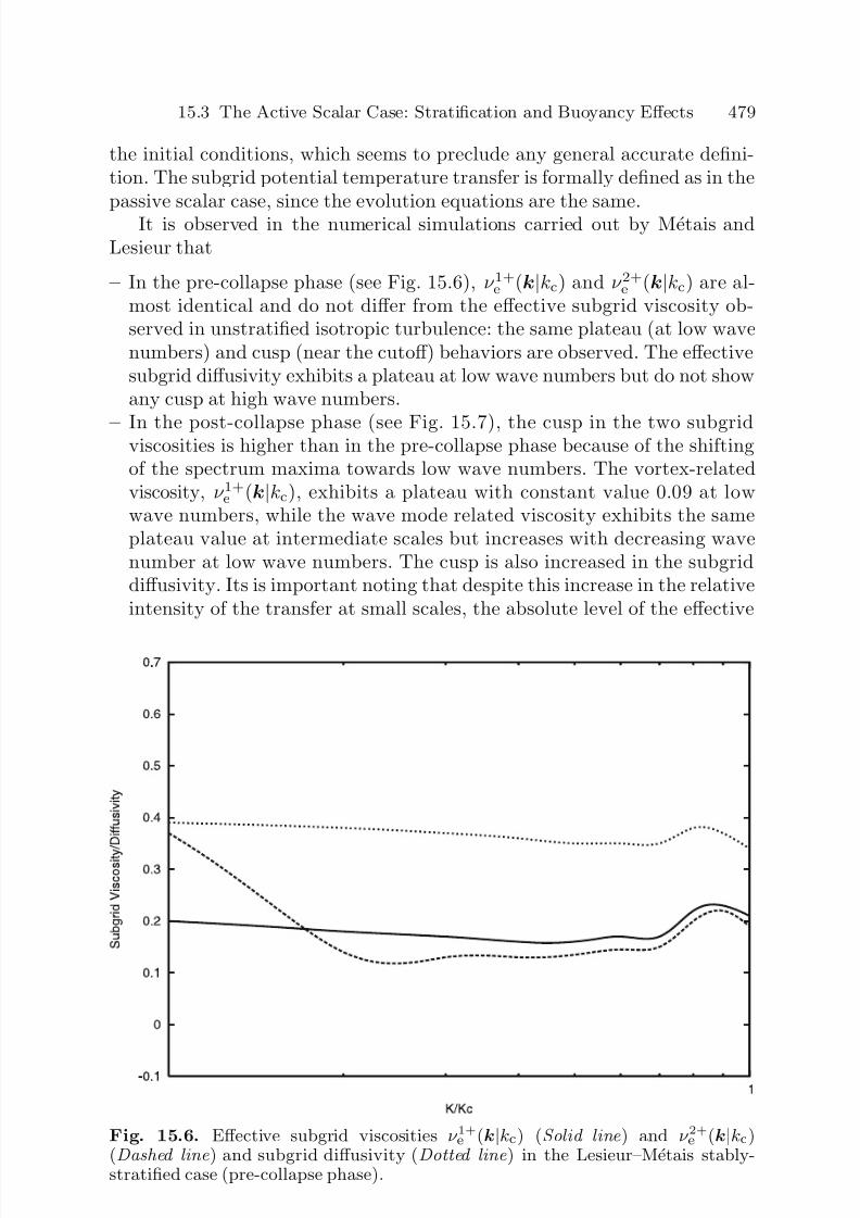
7/21/2019 Large Eddy Simulation for Incompressible Flows
http://slidepdf.com/reader/full/large-eddy-simulation-for-incompressible-flows 497/573
15.3 The Active Scalar Case: Stratification and Buoyancy Effects 479
the initial conditions, which seems to preclude any general accurate defini-tion. The subgrid potential temperature transfer is formally defined as in thepassive scalar case, since the evolution equations are the same.
It is observed in the numerical simulations carried out by Metais andLesieur that
– In the pre-collapse phase (see Fig. 15.6), ν 1+e (k|kc) and ν 2+
e (k|kc) are al-most identical and do not differ from the effective subgrid viscosity ob-served in unstratified isotropic turbulence: the same plateau (at low wavenumbers) and cusp (near the cutoff) behaviors are observed. The effectivesubgrid diffusivity exhibits a plateau at low wave numbers but do not showany cusp at high wave numbers.
– In the post-collapse phase (see Fig. 15.7), the cusp in the two subgridviscosities is higher than in the pre-collapse phase because of the shiftingof the spectrum maxima towards low wave numbers. The vortex-relatedviscosity, ν 1+
e (k|kc), exhibits a plateau with constant value 0.09 at lowwave numbers, while the wave mode related viscosity exhibits the sameplateau value at intermediate scales but increases with decreasing wavenumber at low wave numbers. The cusp is also increased in the subgriddiffusivity. Its is important noting that despite this increase in the relativeintensity of the transfer at small scales, the absolute level of the effective
Fig. 15.6. Effective subgrid viscosities ν 1+e (k|kc) (Solid line ) and ν 2+e (k|kc)(Dashed line ) and subgrid diffusivity (Dotted line ) in the Lesieur–Metais stably-stratified case (pre-collapse phase).
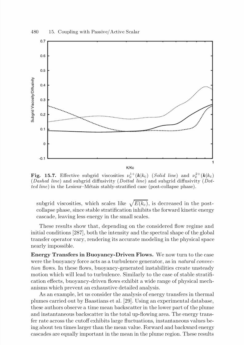
7/21/2019 Large Eddy Simulation for Incompressible Flows
http://slidepdf.com/reader/full/large-eddy-simulation-for-incompressible-flows 498/573
480 15. Coupling with Passive/Active Scalar
Fig. 15.7. Effective subgrid viscosities ν 1+e (k
|kc) (Solid line ) and ν 2+e (k
|kc)
(Dashed line ) and subgrid diffusivity (Dotted line ) and subgrid diffusivity (Dot-ted line ) in the Lesieur–Metais stably-stratified case (post-collapse phase).
subgrid viscosities, which scales like
E (kc), is decreased in the post-collapse phase, since stable stratification inhibits the forward kinetic energycascade, leaving less energy in the small scales.
These results show that, depending on the considered flow regime andinitial conditions [287], both the intensity and the spectral shape of the global
transfer operator vary, rendering its accurate modeling in the physical spacenearly impossible.
Energy Transfers in Buoyancy-Driven Flows. We now turn to the casewere the buoyancy force acts as a turbulence generator, as in natural convec-tion flows. In these flows, buoyancy-generated instabilities create unsteadymotion which will lead to turbulence. Similarly to the case of stable stratifi-cation effects, buoyancy-driven flows exhibit a wide range of physical mech-anisms which prevent an exhaustive detailed analysis.
As an example, let us consider the analysis of energy transfers in thermal
plumes carried out by Baastians et al. [29]. Using an experimental database,these authors observe a time mean backscatter in the lower part of the plumeand instantaneous backscatter in the total up-flowing area. The energy trans-fer rate across the cutoff exhibits large fluctuations, instantaneous values be-ing about ten times larger than the mean value. Forward and backward energycascades are equally important in the mean in the plume region. These results
7/21/2019 Large Eddy Simulation for Incompressible Flows
http://slidepdf.com/reader/full/large-eddy-simulation-for-incompressible-flows 499/573
15.3 The Active Scalar Case: Stratification and Buoyancy Effects 481
show that a reliable subgrid model should be able to account for backscat-ter, and to distinguish between different regions of the flow, rendering themodeling task even more difficult as in the stably stratified flow case.
But it is important to remark that, in the basic philosophy which un-derlies most of the developments in the field of Large-Eddy Simulation, itis assumed that driving mechanisms must be directly captured. In the caseof buoyancy-driven flows, buoyancy effects should therefore be directly sim-ulated if they are the only source of turbulence production (free convection).In the case of mixed convection or forced convection, the requirement mightbe less stringent since other physical mechanisms are at play. This is whysome authors use unmodified passive scalar models (and usual closures forthe momentume equations) to treat Rayleigh–Benard convection at medium
Prandtl number.
15.3.3 Extensions of Functional Models
We now discuss the most illustrative functional models in the physical spacefor the active scalar case. Since a two-way coupling exists, subgrid models forboth the momentum and the scalar equations must be revisited to account forstratification/buoyancy effects. Modeling strategies based on the definition of scalar subgrid viscosity/diffusivity parameters are first considered (p. 481).Dynamic models based on the Germano identity are presented in the secondpart of the section (p. 486).
Scalar Subgrid Viscosity/Diffusivity Models. The brief review of re-sults dealing with interscale energy transfers in flows with active scalar givenin the previous section obviously shows that they are strongly affected in bothstable and unstable stratification cases. This is why most scalar models are de-rived considering a simplified kinetic energy balance equation which includesbuoyancy effects. The most popular simplified energy balance expression is
obtained by neglecting all diffusive and convective effects in (15.89), yieldingan extended local equilibrium (production = dissipation) assumption:
ε = −τ : S − b · τ θ, b ≡ 1
Θ0g , (15.101)
where it is recalled that ε, τ and τ θ are the subgrid kinetic energy dissipationrate, the momentum subgrid tensor and the potential temperature subgridflux vector, respectively. Now specializing Eq. (15.101) by inserting scalarfunctional models of the form
τ = −2ν sgsS, τ θ = −κsgs∇θ , (15.102)
one obtains
ν sgs|S |2 − κsgsN 2c = ε , (15.103)

7/21/2019 Large Eddy Simulation for Incompressible Flows
http://slidepdf.com/reader/full/large-eddy-simulation-for-incompressible-flows 500/573
482 15. Coupling with Passive/Active Scalar
where the local parameter N 2c is defined as
N
2
c ≡ −b · ∇θ =
g
Θ0
∂θ
∂z , (15.104)
and can be either positive or negative. Negative (resp. positive) values areassociated with a decrease (resp. increase) of the subgrid kinetic energy dis-sipation rate by the buoyancy effects.
Equation (15.103) shows that the two-way coupling observed in the activescalar case precludes any decoupled definitions for ν sgs and κsgs.
Now assuming that the cutoff is located within an inertial-convective-likerange, dimensional analysis yields
ν sgs = C ν |ε|1/3∆4/3, κsgs = C κ|ε|1/3∆4/3 , (15.105)
where C ν and C κ are positive parameters. The combination of (15.103)and (15.105) leads to the following expression for the dissipation rate:
ε = |ε|1/3∆4/3
C ν |S |2 − C κN 2c
. (15.106)
This expression leads to the following definition for the subgrid viscosityand the subgrid diffusivity:
ν sgs = C ν ∆2 C ν |S |2 − C κN 2c
1/2= C ν ∆
2|S |2 − N 2c
P rsgs
1/2
T
, (15.107)
κsgs = C κ∆2 C ν |S |2 − C κN 2c
1/2= C κ∆
2|S |2 − N 2c
P rsgs
1/2
T
, (15.108)
where the subgrid Prandtl number is defined as P rsgs ≡ C ν /C κ = C ν /C κ.The main modification with respect to the passive scalar lies in the evaluationof the characteristic time scale T −1: it now combines the velocity gradientand the buoyancy effects. Model (15.107) can be seen as an extension of theclassical Smagorinsky subgrid viscosity model (5.90). It is seen that stablestratification, which is associated with positive values of N 2c , correspondsto a decrease of the subgrid viscosity and diffusivity. This is in agreementwith results dealing with the evolution of subgrid transfers discussed above.
Unstable stratification corresponds to an increase of subgrid viscosity anddiffusivity, in agreement with the physical picture that the forward kineticenergy cascade is enhanced since the subgrid kinetic energy is increased.
The subgrid time scale in (15.107) and (15.108) is defined as an absolutevalue and leads to the definition of positive subgrid parameters. The reasonis that the rough estimates used to obtain the expressions given above do not
7/21/2019 Large Eddy Simulation for Incompressible Flows
http://slidepdf.com/reader/full/large-eddy-simulation-for-incompressible-flows 501/573
15.3 The Active Scalar Case: Stratification and Buoyancy Effects 483
ensure that realizability is enforced, i.e. that the energy destroyed by stabiliz-ing stratification effects is smaller than the available subgrid kinetic energy.But when the backscatter is dominant, the definition is no longer relevantto account for subgrid transfers if the subgrid Prandtl number is kept posi-tive. In this case, Eidson [209] proposes to clip negative values of N 2c so thatT remains well-posed. A simple solution is to consider N 2+
c = max(0, N 2c ).The resulting subgrid viscosity model can be rewritten as a function of theoriginal Smagorinsky model (5.90):
ν sgs = C ν ∆2|S |
Smagorinsky
1 − 1
P rsgs
N 2+c
|S |2 . (15.109)
This modified expression can be recast in a form which emphasizes therole of the Richardson number [690]:
ν sgs = C ν ∆2|S |
Smagorinsky
1 − Ri
Riref , (15.110)
where the local subgrid Richardson number Ri is defined as Ri = N 2+c /|S |2
and Riref
≡P rsgs is a reference value. This new expression also illustrates the
physical meaning of the subgrid Prandtl number in stably stratified flows.A modified evaluation of the time scale is proposed by Peng and David-
son [587], which is always well-posed from a mathematical standpoint:
T =
|S | − N 2c
|S |P rsgs
. (15.111)
A more general scalar model is proposed by Schumann, which containsan anisotropic residual heat flux associated to buoyancy effects. It is derived
considering simplified evolution equation for the subgrid stresses and subgridheat fluxes and assuming that the local equilibrium applies, yielding
τ = −2C ν ∆2T S, τ θ = −C κ∆
2T (b∇θ) , (15.112)
where the time scale T −1 and the tensor b are defined as
b = I d + C 2
T 2 + C 2N 2cb∇θ , (15.113)
T 2 = 12 |S |2 − (C 1 + C 2)N 2c + 14 |S |2 − (C 1 − C 2)N 2c 2 + C 1C 2N 4m ,
(15.114)where N 2c is given by (15.104) and
N 2m =
(b · b)(∇θ · ∇θ) . (15.115)

7/21/2019 Large Eddy Simulation for Incompressible Flows
http://slidepdf.com/reader/full/large-eddy-simulation-for-incompressible-flows 502/573
484 15. Coupling with Passive/Active Scalar
Table 15.1. Values of the constants in buoyancy-affected subgrid models.
Model C 1 C 2
Passive scalar 0 0Buoyant 1/P rsgs 0Eidson 2.5 0.Schumann 2.5 3.
As noted by Cabot [85], this general model encompasses the previousones. Corresponding values of the constants C 1 and C 2 are summarized inTable 15.1.
The Schumann model appears to be the most complex one, and includesmore information related to anisotropy. It is therefore expected that it shouldyield better results in buoyancy-driven flows with high Prandtl numbers.
More complex models relying on the definition of tensorial subgrid vis-cosity/diffusivity to account for anisotropy can also be defined. Such models,very similar to the one proposed by Yoshizawa for the passive scalar case(Sect. 15.2.3, p. 465) were tested by Peng and Davidson [587] for buoyancy-driven flows. These authors use the following expression for the subgrid heatflux
τ G(ui, θ) = −CT sgsτ G(ui, uk) ∂θ∂xk
, (15.116)
where C is a constant, T sgs and appropriate time scale and the subgrid mo-mentum flux is modeled by an ad hoc model. In the case a subgrid-viscositytype model is considered for τ G(u, u) and the cascade time scale is evaluated
as T sgs = ∆2
/ν sgs, the resulting model is
τ G(ui, θ) = −C∆2
S ik∂θ
∂xk
. (15.117)
The value of the subgrid viscosity can be modified accounting for thisexpression in the following way. Starting from the local equilibrium hypoth-
esis (15.101) and approximating the subgrid dissipation rate as ε ∝ ν 3sgs/∆4
,one obtains
ν sgs = C ∆2
|S |2 − 1
ν sgs
giΘ0
τ G(ui, θ) . (15.118)
Now using (15.116), one obtains the following evaluation of the subgrid
viscosity
ν sgs = C ∆2
|S |2 − γ
|S |giΘ0
S ik∂θ
∂xk, (15.119)
where C and γ are adjustable parameters, which can be computed usinginertial-range considerations or a dynamic procedure.

7/21/2019 Large Eddy Simulation for Incompressible Flows
http://slidepdf.com/reader/full/large-eddy-simulation-for-incompressible-flows 503/573
15.3 The Active Scalar Case: Stratification and Buoyancy Effects 485
All functional models presented above are built on the same bases, andare based on the resolved strain. They can be interpreted as extensions of theSmagorinsky model. Another class of models, which is very popular amongresearchers working in the field of meteorology, is the one of models based onthe subgrid kinetic energy:
ν sgs = C ν l
q 2sgs, κsgs = C κl
q 2sgs , (15.120)
where C ν and C κ are constants and l a characteristic length scale. The subgridkinetic energy must be evaluated using a prognostic equation or a simplifiedapproximation (see Sect. 15.3.5). Since the time scale T does not appearexplicitely in these expressions, the stratification effect must be taken intoaccount in the definition of the length scale l. The subgrid Prandtl numberassociated with this corrected length scale is
P rsgs = ∆
∆ + 2l. (15.121)
In the case of unstable stratification, the length scale is taken equal to itsusual value tied to the filter cutoff, i.e. l = ∆. In the case of stably stratifiedflows, a first simple model proposed by Schumann for meteorology-related
purpose is
l = min
∆, LN
, LN = 0.76
q 2sgs
N 2c. (15.122)
A more general corrected expression, which accounts for both stable strat-ification and shear effects is proposed by Canuto and Cheng [99]. It is writtenas follows:
l = ∆f (|S |, N c) , (15.123)
with
f (|S |, N c) =
1
0
[1 − X log(1 + aQ2)]2dQ3/2
, (15.124)
X =
√ 3
16 K
3/20
P rsgsS 2h
F r2i
− 1
, a =
2
π2F r2i f (|S |, N c)
2/3,
Q = (k∆/π)2/3 , (15.125)
where the non-dimensional shear number and the inverse Froude number aredefined as
S h = ∆|S |
q 2sgs
, F ri = ∆N c
q 2sgs
. (15.126)

7/21/2019 Large Eddy Simulation for Incompressible Flows
http://slidepdf.com/reader/full/large-eddy-simulation-for-incompressible-flows 504/573
486 15. Coupling with Passive/Active Scalar
Dynamic Models. A weakness shared by all the models presented above isthe existence of preset constants. They can be evaluated using inertial rangeconsiderations, or they can be automatically adjusted using a dynamic proce-dure. The use of a dynamic procedure based on the Germano identity yieldsmuch more difficult problems than in other cases, because of the intrinsiccoupling between the momentum and the temperature subgrid fluxes. Thisproblem is clearly seen considering the following generic closures
τ ij = C ν f ij(∆, u, θ , P rsgs), τ θi = C ν P rsgs
hi(∆, u, θ , P rsgs) . (15.127)
The two unknown parameters are C ν and P rsgs. Inserting these expres-
sions in the Germano identities for the momentum and temperature fluxesand using the classical assumptions, one defines the two following residuals:
E ij = Lij − C ν
f ij(
∆, u,θ , P rsgs) − f ij(∆,u,θ,Prsgs)
, (15.128)
E θi = hi − C ν P rsgs
hi(∆, u,θ , P rsgs) − hi(∆,u,θ,Prsgs)
. (15.129)
The two unknown parameters are chosen so as to minimize the globalerror in the least square sense, leading to the definition of four constraints:
∂ E : E ∂C ν
= 2E : ∂ E ∂C ν
= 0, ∂ E : E
∂P rsgs= 2E : ∂ E
∂P rsgs= 0 , (15.130)
∂ E θ : E θ∂C ν
= 2E θ : ∂ E θ∂C ν
= 0, ∂ E θ : E θ
∂P rsgs= 2E θ :
∂ E θ∂P rsgs
= 0 . (15.131)
The complexity of this problem is enlightened looking at the definition of the subgrid Prandtl number: since both f ij and hi are non linear functions of
P rsgs, the use of either (15.130) or (15.131) leads to the definition of a systemof non-linear equations for it, which cannot be solved explicitely as in previouscases. Thus, the dynamic evaluation of the constants now require to solvea non linear system, leading to a subsequent increase in the computationalcomplexity. It also raises the problem of finding the best among the multiplepossible roots of the system.
This is why many authors use the same dynamic models as in the passivescalar case (i.e. with basic models which are linear with respect to the subgridPrandtl number), with the idea that, if the grid is fine enough, most of thestratification effects will be captured. This is especially true of the stablestratification effects, where the decrease in the subgrid energy transfer maybe partially captured using a dynamic procedure, since resolved scales arealready affected. The case of buoyancy driven flows is much more difficult,since turbulence production exist at small scales which cannot be inferredfrom the resolved scale dynamics. Therefore, the use of purposely modified
7/21/2019 Large Eddy Simulation for Incompressible Flows
http://slidepdf.com/reader/full/large-eddy-simulation-for-incompressible-flows 505/573
15.3 The Active Scalar Case: Stratification and Buoyancy Effects 487
models for buoyancy-driven flows is more important than in the case of stablestratification.
15.3.4 Extensions of Structural Models
We now consider structural models. As in the passive scalar case, modelsrelying on the explicit evaluation of subgrid scales (soft deconvolution models,scale similarity models, linear combination models [19], explicit stochastic ordeterministic models for subgrid fluctuations, multilevel simulations) can beused in a straightforward way, since they do not rely on any assumptionsdealing with the nature of subgrid transfers. Consequently, these models willnot be explicitly detailed in this section, since they don’t need to be modifiedto account for the active scalar dynamics. Another comment is that manystructural models have not yet been tested in stably/unstably stratified flows.
In this section, we will put the emphasis on models which contain explicitmodifications and whose accuracy has already been assessed in real Large-Eddy Simulations:
– Deardorff’s differential stress model (p. 487), which requires to solve tenadditional transport equations.
– Schumann’s algebraic stress model (p. 488), wich can be seen as a simplifi-
cation of the previous model and necessitates to solve only one additionalprognostic equation to compute the subgrid kinetic energy.
Deardorff Differential Model. The differential model proposed by Dear-dorff [173] relies on solving closed expressions of (15.88) and (15.90).
In the equations for the subgrid momentum fluxes (15.88), the only newterms with respect to the case treated in Sect. 7.5.1 is the coupling term.Since the closures proposed by Deardorff are kept unmodified in the activescalar case, all the dynamic coupling effects are contained in the couplingterm. Since this term is directly proportional to the subgrid heat fluxes which
are explicitely computed, no further closure assumptions is needed for theseequations.
The equations for the subgrid scalar fluxes and the associated closureshave already been discussed in Sect. 15.2.4. Among already closed terms inthe passive scalar case, only the pressure-temperature term is modified toaccount for stratification effects: Equation (15.60) is changed into
τ G
θ,
∂p
∂xi= −C 1
q 2sgs
∆τ G(ui, θ) − 1
3biτ G(θ, θ) , (15.132)
which necessitates an evaluation of the generalized subgrid scalar variance,τ G(θ, θ). The new term appearing in (15.90) is the coupling term, which isalso proportional to the generalized subgrid scalar variance.
Therefore, an additional prognostic equation for τ G(θ, θ) deduced from(15.8) is solved. Term V II is directly computed, since the subgrid scalar
7/21/2019 Large Eddy Simulation for Incompressible Flows
http://slidepdf.com/reader/full/large-eddy-simulation-for-incompressible-flows 506/573
488 15. Coupling with Passive/Active Scalar
fluxes are explicitly computed. Molecular diffusion IX , is neglected, whilethe molecular dissipation IX is evaluated as
2κτ G
∂θ
∂xk,
∂θ
∂xk
= C IX
q 2sgs
∆τ G(θ, θ), C IX = 0.42 , (15.133)
while the subgrid diffusion cubic term X is closed as
τ G(uk, θ , θ) = −C X∆
q 2sgs
∂
∂xkτ G(θ, θ), C X = 0.2 . (15.134)
The resulting solvable equation for the subgrid temperature variance is
∂τ G(θ, θ)
∂t + uk
∂τ G(θ, θ)
∂xk= −2τ G(uk, θ)
∂θ
∂xk− C IX
q 2sgs
∆τ G(θ, θ)
+C X∂
∂xk
∆
q 2sgs
∂
∂xkτ G(θ, θ)
,(15.135)
achieving the description of the model.
Schumann Algebraic Stress Model. A much simpler model, which doesnot require to solve a large amount of additional transport equations, was
developed by Schmidt and Schumann [651] to analyze the convective bound-ary layer dynamics. This model can be interpreted as a simplification of theDeardorff model, in which several contributions will be neglected.
Starting from (15.88) and making the following assumptions:
1. The subgrid fluxes respond instantaneously to large-scale forcing, i.e. thetime derivative term is negligible.
2. Diffusive terms are small, and can be neglected.3. Importance of the deviatoric part of the subgrid stress tensor in the
production terms is small, with respect to the one of the isotropic part.4. The pressure-velocity term can be modeled as
τ G
p,
∂ui∂xk
= C 1q 2sgsS ik − C 2
q 2sgs
∆τ ∗G(ui, uj) + C 3
g
Θ0
×
τ G(ui, θ)δ k3 + τ G(uk, θ)δ i3 − 2
3τ G(u3, θ)δ ij
,
(15.136)
where C 1, C 2 and C 3 are model parameters. The star superscript denotesthe deviatoric part of the tensor.5. The subgrid dissipation term is approximated as
2ντ G
∂uj∂xk
, ∂ui∂xk
=
2
3q 2sgsS ij . (15.137)

7/21/2019 Large Eddy Simulation for Incompressible Flows
http://slidepdf.com/reader/full/large-eddy-simulation-for-incompressible-flows 507/573
15.3 The Active Scalar Case: Stratification and Buoyancy Effects 489
one obtains the following linear relationship for the subgrid stresses:
C Rm q 2sgs
∆τ ∗G(ui, uj) = (1 − C Bm) g
Θ0× τ G(ui, θ)δ k3 + τ G(uk, θ)δ i3
−2
3τ G(u3, θ)δ ij
− (1 − C Gm)
2
3q 2sgsS ij ,
(15.138)
where C Rm = 3.5, C Bm = 0.55 and C Gm = 0.55. The subgrid heat fluxes areknown since they are also outputs of the model, and the subgrid kinetic energyis obtained solving a prognostic equation derived from (15.89). Since the exact
equation differs from the one associated to the unstratified case only becauseof the coupling term, and that this coupling term is directly proportionalto the subgrid heat flux which is an output of the model, a simple solutionconsists in using the same closed equation as in the unstratified case (seeSect. 5.4.2, p. 173) with the additional coupling term. More complex variantsof the prognostic equation for the subgrid kinetic energy are presented ina dedicated section (Sect. 15.3.5).
The subgrid heat flux equation (15.90) is simplified using similar assump-tions:
1. The time derivative is negligible.2. Convective and diffusive fluxes are negligible.3. The dissipation term is negligible.4. Contribution of the deviatoric part of the subgrid stress tensor in the
production term is very small compared to the one of its isotropic part.5. The pressure-temperature subgrid flux can be modeled as
ντ G p, ∂θ
∂xi = 2a1q 2sgs
∂θ
∂xi −a2
√ 2
q 2sgs
∆
τ G(θ, ui)
+ 2a3g
Θ0τ G(θ, θ)δ i3 , (15.139)
with ai are adjustable parameters.
The resulting algebraic equation is
C Rθ
q 2sgs
∆δ ik +
∂ui∂xk
τ G(θ, uk) = −2
3(1 − C Gθ)q 2sgs
∂θ
∂xi
+ (1 + C Bθ) g
Θ0τ G(θ, θ)δ i3 . (15.140)
To obtain a fully explicit model for the subgrid heat flux, it is necessaryto eliminate the term related to the resolved velocity gradient in the left hand

7/21/2019 Large Eddy Simulation for Incompressible Flows
http://slidepdf.com/reader/full/large-eddy-simulation-for-incompressible-flows 508/573
490 15. Coupling with Passive/Active Scalar
side, i.e. to neglect production effects associated with the interaction of thesubgrid heat flux with the resolved velocity gradient, yielding
C Rθ
q 2sgs
∆τ G(θ, ui) = −2
3(1 − C Gθ)q 2sgs
∂θ
∂xi+ 2(1 − C Bθ)
g
Θ0τ G(θ, θ)δ i3 .
(15.141)The constants are set equal to: C Rθ = 1.63, C Gθ = 0.5, C Bθ = 0.5. The
subgrid scalar variance equation is simplified using a local equilibrium hy-pothesis, leading to the following explicit expression
C εθ q 2sgs
∆ τ G(θ, θ) = 2τ G(θ, ui)
∂θ
∂xi , (15.142)
with C εθ = 2.02. The explicit model is obtained by solving (15.138), (15.141)and (15.142) supplemented with a prognostic equation for the subgrid kineticenergy. Therefore, it appears much more simple than a differential stressmodel. Another interesting feature of this model is that it do not rely onthe eddy diffusivity/viscosity paradigm and is fully anisotropic. Nevertheless,since it is based on strong assumptions, its domain of validity is expected tobe narrower than the one of the full differential model.
In the absence of buoyancy, the model simplifies as a simple subgrid vis-cosity/subgrid diffusivity model:
ν sgs = C ν ∆
q 2sgs, κsgs = C κ∆
q 2sgs , (15.143)
with
C ν = 2
3
1 − C GmC Rm
, C κ = 2
3
1 − C GθC Rθ
. (15.144)
The corresponding value of the subgrid Prandtl number is
P rsgs = β
2K 0. (15.145)
15.3.5 Subgrid Kinetic Energy Estimates
The modeled prognostic equation for the subgrid kinetic energy q 2sgs ≡12 τ G(ui, ui) can be modified to account for buoyancy/stratification effects
[402]. Rewritting the transport equation for this quantity as
∂q 2sgs
∂t + uj
∂q 2sgs
∂xj= P − D − ε +
g
Θ0τ G(u3, θ) , (15.146)
7/21/2019 Large Eddy Simulation for Incompressible Flows
http://slidepdf.com/reader/full/large-eddy-simulation-for-incompressible-flows 509/573
15.3 The Active Scalar Case: Stratification and Buoyancy Effects 491
where the production P and the diffusion D are defined as
P =
−τ : S, D =
∇ ·(uq 2sgs + pId) , (15.147)
and where ε is the dissipation rate. The model for the production term andthe diffusion term are not modified to account for active scalar dynamics
P = C e∆
q 2sgs|S |2 , (15.148)
D = −2C e∂
∂xk
∆
q 2sgs
∂q 2sgs
∂xk
, (15.149)
where C e is a constant. The subgrid kinetic energy dissipation rate is modifiedto account for stabilizing stratification effects by writing it as
ε = C e
q 2sgs
3/2
Lε, (15.150)
where the characteristic dissipative length scale Lε is defined as
Lε = 1
∆
2 + 1
L2
N
+ 1
L2
S −1/2
. (15.151)
The subgrid buoyancy lenghtscale, LN , and the subgrid shear length scale,LS , are defined as
LN = 0.76
q 2sgs
N 2c, LS = 2.76
q 2sgs
|S |2 , (15.152)
where N 2c is defined as in (15.104). This expression was derived to accountfor the dynamics of a shear-driven stable atmospheric boundary layer. The
predicted value of the dissipation length scale is larger or equal to ∆, yield-ing a decrease of the predicted dissipation, in agreement with the observeddiminution in the forward kinetic energy cascade rate.
An algebraic expression which takes into account the correction in thedefinition of the dissipation length scale is obtained by assuming that thedissipation is locally balanced by conversion of the mean flow energy intosubgrid kinetic energy (production = dissipation):
ε = P − D . (15.153)
Using (15.150) and (15.103), one obtains
q 2sgs =
LεC e
ν sgs|S |2 − κsgsN 2c
2/3
. (15.154)

7/21/2019 Large Eddy Simulation for Incompressible Flows
http://slidepdf.com/reader/full/large-eddy-simulation-for-incompressible-flows 510/573
492 15. Coupling with Passive/Active Scalar
This equation is fully non-linear if models based on the subgrid kineticenergy are used for the subgrid viscosity and the subgrid diffusivity, and/or if the corrected model for Lε is utilized. In the absence of stability correction forthe dissipation length scale, and using the following subgrid kinetic energy-based models:
ν sgs = C ν ∆
q 2sgs, κsgs = C κ∆
q 2sgs , (15.155)
one obtains the following explicit algebraic expression [690]:
q 2sgs = ∆
2
C e C ν |S |2 − C κN 2c . (15.156)
More expressions for the subgrid kinetic energy can be found using othermodels for the subgrid viscosity and diffusivity.
15.3.6 More Complex Physical Models
The active scalar model discussed above can be further complexified to ac-count for more complex physics. This is currently done in studies dealingwith the atmospheric boundary layer, in which detailed microphysical mod-
els (icing, moisture) and infrared radiative cooling are taken into account.The related subgrid models are made more complex to account for new phys-ical mechanisms. They are nor presented here, since they are very specificto the field of application. The interested reader can refer to the originalpublications.
15.3.7 A Few Applications
Stably stratified flows:
– Stably stratified channel flow [19, 195, 238]– Forced homogeneous stably stratified turbulence [110]– Decaying homogeneous stably stratified flows [514, 373]– Turbulent penetrative convection [124]– Wake in a weakly stably stratified fluid [194]
Buoyancy-driven flows:
– Thermal plume [29, 28]
– Turbulent penetrative convection [124]– Buoyancy-generated homogeneous turbulence [123]– Rayleigh–Benard convection [209, 394, 766, 85, 575]– Rotating Rayleigh–Benard flow [152]– Forced and mixed convection in rotating and non-rotating square duct [577]– Natural convection in a cavity [586, 800]

7/21/2019 Large Eddy Simulation for Incompressible Flows
http://slidepdf.com/reader/full/large-eddy-simulation-for-incompressible-flows 511/573
15.3 The Active Scalar Case: Stratification and Buoyancy Effects 493
– Turbulent convection driven by free-surface cooling [814]– Buoyant jet [808]– Buoyant wake [539]– Buoyant pipe flow [433]
Meteorology-related applications: [601, 488, 525, 444, 698, 651, 130, 656,173, 402, 277, 690, 337, 615, 109, 154, 111, 527, 534, 528, 317, 657, 529, 658,530, 450, 699, 697, 690, 638, 526, 532, 531]
7/21/2019 Large Eddy Simulation for Incompressible Flows
http://slidepdf.com/reader/full/large-eddy-simulation-for-incompressible-flows 512/573
A. Statistical and Spectral Analysisof Turbulence
A.1 Turbulence Properties
Flows qualified as “turbulent” can be found in most fields that make use of fluid mechanics. These flows posses a very complex dynamics whose intimatemechanisms and repercussions on some of their characteristics of interest tothe engineer should be understood in order to be able to control them. Thecriteria for defining a turbulent flow are varied and nebulous because thereis no true definition of turbulence. Among the criteria most often retained,we may mention [150]:
– the random character of the spatial and time fluctuations of the veloci-
ties, which reflect the existence of finite characteristic scales of statisticalcorrelation (in space and time);
– the velocity field is three-dimensional and rotational;– the various modes are strongly coupled, which is reflected in the non-
linearity of the mathematical model retained (Navier–Stokes equations);– the large mixing capacity due to the agitation induced by the various scales;– the chaotic character of the solution, which exhibits a very strong depen-
dency on the initial condition and boundary conditions.
A.2 Foundations of the Statistical Analysisof Turbulence
A.2.1 Motivations
The very great dynamical complexity of turbulent flows makes for a verylengthy deterministic description of them. To analyze and model them, weusually refer to a statistical representation of the fluctuations. This reduces
the description to that of the various statistical moments in the solution,which sharply reduces the volume of information. Moreover, the random char-acter of the fluctuations make this approach natural.
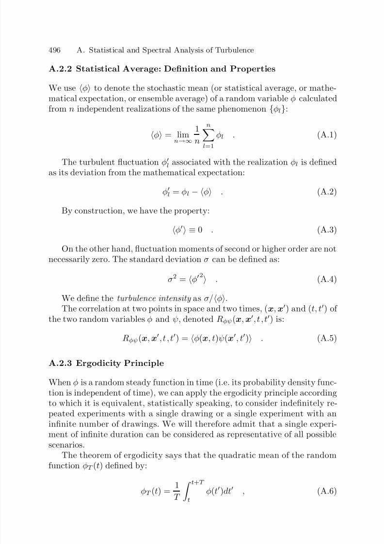
7/21/2019 Large Eddy Simulation for Incompressible Flows
http://slidepdf.com/reader/full/large-eddy-simulation-for-incompressible-flows 513/573
496 A. Statistical and Spectral Analysis of Turbulence
A.2.2 Statistical Average: Definition and Properties
We use
φ
to denote the stochastic mean (or statistical average, or mathe-
matical expectation, or ensemble average) of a random variable φ calculatedfrom n independent realizations of the same phenomenon φl:
φ = limn→∞
1
n
nl=1
φl . (A.1)
The turbulent fluctuation φl associated with the realization φl is definedas its deviation from the mathematical expectation:
φl = φl − φ . (A.2)
By construction, we have the property:
φ ≡ 0 . (A.3)
On the other hand, fluctuation moments of second or higher order are notnecessarily zero. The standard deviation σ can be defined as:
σ2 =
φ
2
. (A.4)
We define the turbulence intensity as σ/φ.The correlation at two points in space and two times, (x, x) and (t, t) of
the two random variables φ and ψ, denoted Rφψ(x, x, t , t) is:
Rφψ(x, x, t , t) = φ(x, t)ψ(x, t) . (A.5)
A.2.3 Ergodicity Principle
When φ is a random steady function in time (i.e. its probability density func-tion is independent of time), we can apply the ergodicity principle accordingto which it is equivalent, statistically speaking, to consider indefinitely re-peated experiments with a single drawing or a single experiment with aninfinite number of drawings. We will therefore admit that a single experi-ment of infinite duration can be considered as representative of all possiblescenarios.
The theorem of ergodicity says that the quadratic mean of the randomfunction φT (t) defined by:
φT (t) = 1
T
t+T t
φ(t)dt , (A.6)

7/21/2019 Large Eddy Simulation for Incompressible Flows
http://slidepdf.com/reader/full/large-eddy-simulation-for-incompressible-flows 514/573
A.2 Foundations of the Statistical Analysis of Turbulence 497
converges to a non-random limit equal to the stochastic mean φ as T → ∞only on the condition that:
limT →∞
1T T
0
Rφφ(t)dt = 0 , (A.7)
where Rφφ(t) is the time autocorrelation (or covariance) of the fluctuationsof φ over time interval t:
Rφφ(t) = (φ(t) − φ)(φ(t + t) − φ) . (A.8)
For turbulent fluctuations, the random character reflects the fact thatRφφ(t)
→0 as t
→ ∞. So if we define the mean in time φ as the limit of φT
as T → ∞, i.e.:
φ = limT →∞
1
T
T 0
φ(t)dt , (A.9)
we get the equality:φ = φ . (A.10)
We establish that the standard error varies as 1/√
T for sufficientlylarge T . Another way of estimating φ is to construct the “experimental”average φn defined as the arithmetic mean from experiments:
φn(t) = 1
n
ni=1
φi(t) , (A.11)
where the time t is arbitrary since the flow is assumed to be statisticallysteady. We show that the standard error decreases as 1/
√ n if the experiments
φl are independent.Let φ and ψ be two random variables. The operator thus defined verifies
the following properties, sometimes called Reynolds rules:
φ + ψ = φ + ψ , (A.12)
aφ = aφ a = const. , (A.13)
φψ = φψ , (A.14)∂φ
∂s
=
∂ φ∂s
s = x, t , (A.15)
φ(x, t)d3xdt
=
φ(x, t)d3xdt . (A.16)
Any operator that verifies these properties is called a Reynolds operator.We deduce from these relations the properties:
φ = φ , (A.17)
φ = 0 . (A.18)

7/21/2019 Large Eddy Simulation for Incompressible Flows
http://slidepdf.com/reader/full/large-eddy-simulation-for-incompressible-flows 515/573
498 A. Statistical and Spectral Analysis of Turbulence
A.2.4 Decomposition of a Turbulent Field
Decomposition Principle. One technique very commonly used for describ-
ing a turbulent field is statistical representation. The velocity field at time tand position x splits into:
u(x, t) = u(x, t) + u(x, t) . (A.19)
Using this decomposition and the stochastic mean, we define an evolutionequation for the quantity u(x, t). To recover all the information containedin the u(x, t) field, we have to handle an infinite set of equations for thestatistical moments of it. The quadratic non-linearity of the Navier–Stokes
equations induces an intrinsic coupling among the various moments of thesolution: the evolution equation of the moment of order n in the solutionuses the moment of order (n + 1). To recover all the information in theexact solution, it is thus necessary to solve an infinite hierarchy of coupledequations. As this is impossible in practice, this hierarchy is truncated atan arbitrarily chosen level so as to obtain a finite number of equations. Thistruncation brings out an unknown term that will be modeled using closurehypotheses. If the degree of precision of the information obtained theoreticallyincreases with the number of equations retained, the consequences of the
truncation and of the hypotheses used are difficult to predict.Equations of the Stochastic Moments. The evolution equations of themean field are obtained by applying the averaging operator to the Navier–Stokes equations. By applying the rules of commutation with the derivationin the case of an incompressible Newtonian fluid and with no external forces,we get
∂ ui∂t
+ ∂
∂xjuiuj = −∂ p
∂xi+ ν
∂ 2u∂xj∂xj
, (A.20)
∂ ui
∂xi = 0 , (A.21)
where ν is the kinematic viscosity. The non-linear term uiuj is unknownand has to be decomposed as a function of u and u. By introducing rela-tion (A.19) and considering the properties (A.12) to (A.18), we get:
uiuj = uiuj + uiuj . (A.22)
The last term of the right-hand side, called the Reynolds tensor, is un-known and has to be evaluated. It represents the coupling between the fluc-tuations and the mean field. This evaluation can be made by solving thecorresponding evolution equation, either by employing a model, called clo-sure or turbulence model.

7/21/2019 Large Eddy Simulation for Incompressible Flows
http://slidepdf.com/reader/full/large-eddy-simulation-for-incompressible-flows 516/573
A.3 Introduction to Spectral Analysis of the Isotropic Turbulent Fields 499
A.2.5 Isotropic Homogeneous Turbulence
Definitions. A field is said to be statistically homogeneous along the pa-
rameter x, or imprecisely just “homogeneous”, if its statistical moments areindependent of the value of x where the measurements are made. This isexpressed:
∂
∂xφ1....φn = 0 . (A.23)
A homogeneous field is said to be statistically isotropic (in the Taylorsense), or more simply “isotropic”, if all statistical moments relative to a setof points (x1,...,xn) at times (t1,...,tn) remains invariant when the set of npoints and the coordinate axis are rotated, and if there is statistical invariance
for symmetry about an arbitrary plane.We may note that there exists an idea of quasi-isotropy introduced byMoffat, which does not require the invariance by symmetry.
A Few Properties. A turbulent field is said to be homogeneous (resp.homogeneous isotropic) if its velocity fluctuation u is homogeneous (resp.homogeneous isotropic). One necessary condition for achieving homogeneityis that the mean velocity gradient be constant in space:
∂ ui∂xj
= const. (A.24)
Isotropy requires that the mean field u be zero. When the turbulenceis isotropic, only the diagonal elements of the Reynolds tensor are non-zero.Moreover, these are mutually equal:
uiuj =
2
3Kδ ij , (A.25)
where K is the turbulent kinetic energy.
A.3 Introduction to Spectral Analysisof the Isotropic Turbulent Fields
A.3.1 Definitions
The tensor of correlations at two points Rαβ(r) of a statistically homogeneousvector field u defined as:
Rαβ(r) = uα(x + r)uβ(x) (A.26)
can be related to a spectral tensor Φαβ(k) by the following two relations:
Rαβ(r) =
Φαβ(k)eikjrjd3k , (A.27)
Φαβ(k) = 1
(2π)3
Rαβ(r)e−ikjrjd3k , (A.28)

7/21/2019 Large Eddy Simulation for Incompressible Flows
http://slidepdf.com/reader/full/large-eddy-simulation-for-incompressible-flows 517/573
500 A. Statistical and Spectral Analysis of Turbulence
where i2 = −1. The tensor at the origin, Rαβ(0), is the Reynolds tensor.In the case of an isotropic field, the general form of the correlation tensorbecomes:
Rαβ(r) = K [f (r) − g(r)] rαrβr2
+ g(r)δ αβ , (A.29)
where f (r) and g(r) are two real scalar functions. When the velocity field issolenoidal, these two functions are related by:
g(r) = f (r) + r
2
∂f (r)
∂r . (A.30)
The incompressibility constraint also allows us to establish the followingrelation for the tensor Φαβ(k):
Φαβ(k) = E (k)
4πk2
δ αβ − kαkβ
k2
, (A.31)
where the scalar function E (k) is called a three-dimensional spectrum. Itrepresents the contribution of the wave vectors of k to the turbulent kineticenergy, i.e. wave vectors whose tips are included in the region located betweentwo spheres of radius k and k + dk. The spectral energy density, denotedA(k), is therefore equal to E (k)/4πk2. The three-dimensional spectrum is
computed from the spectral tensor by integration over the sphere of radius k:
E (k) = 1
2
Φii(k)dS (k) , (A.32)
where dS (k) is the integration element on the sphere of radius k. This quan-tity can also be related to the function f (r) by the relation:
E (k) = K
π ∞
0
kr (sin(kr) − kr cos(kr)) f (r)dr . (A.33)
The turbulent kinetic energy, K , is found by summation over the entirespectrum:
K ≡ uiui
2 =
∞0
E (k)d3k . (A.34)
By construction, the spectral tensor has the property:
Φij(−k) = Φ∗ij(k) , (A.35)
where the asterisk indicates the complex conjugate number. The homogeneityproperty of the turbulent field implies:
Φij(k) = Φ∗ji(k) . (A.36)

7/21/2019 Large Eddy Simulation for Incompressible Flows
http://slidepdf.com/reader/full/large-eddy-simulation-for-incompressible-flows 518/573
A.3 Introduction to Spectral Analysis of the Isotropic Turbulent Fields 501
The spectral tensor can also be related to the velocity fluctuation u andto its Fourier transform
u defined as:
ui(k) = 1(2π)3 u(x)e−ıkjxjd3x . (A.37)
Simple expansions lead to the equality:
ui(k) uj(k) = δ (k + k)Φij(k) . (A.38)
So we see that the two modes are correlated statistically only if k +k = 0.An equivalent definition of the spectral tensor is:
Φij(k) = u∗i (k) u
j(k)d3k . (A.39)
A.3.2 Modal Interactions
The nature of the interactions among the various modes can be broughtout by analyzing the non-linear term that appears in the evolution equationassociated with them. This equation, for the mode associated with the wavevector k (the dependency on k is not expressed, for the sake of simplicity) is:
∂
ui
∂t + ıkj aij = −ıki p − νk2
ui . (A.40)
The two quantities aij and p are related to uiuj and the pressure p bythe relations:
ui(x)uj(x) =
aij(k)eıklxld3k , (A.41)
1
ρ p(x) =
p(k)eıklxld3k . (A.42)
By introducing the spectral decompositions:
ui(x) = ui(k)eık
lxld3k , (A.43)
uj(x) =
uj(k)eık
l xld3k , (A.44)
the non-linear term becomes:
ui(x)uj(x) =
ui(k) uj(k − k)d3k
aij(k)
eıklxld3k , (A.45)
where we have performed the variable change k = k+ k. The pressure termis computed by the Poisson equation:
1
ρ
∂ 2 p
∂xi∂xi= − ∂ 2uiuj
∂xi∂xj, (A.46)

7/21/2019 Large Eddy Simulation for Incompressible Flows
http://slidepdf.com/reader/full/large-eddy-simulation-for-incompressible-flows 519/573
502 A. Statistical and Spectral Analysis of Turbulence
or, in the spectral space:
k2 p =
−klkm alm . (A.47)
The momentum equation therefore takes the form:∂
∂t + νk2
ui(k) = M ijm(k)
um(k) uj(k − k)d3k , (A.48)
in whichM ijm(k) = − ı
2 (kmP ij(k) + kjP im(k)) , (A.49)
where P ij(k) is the projection operator on the plane orthogonal to the vec-
tor k. This operator is expressed:
P ij(k) =
δ ij − kikj
k2
. (A.50)
The linear terms are grouped into the left-hand side and the non-linearterms in the right. The first linear term represents the time dependency andthe second the viscous effects. The non-linear term represents the effect of convection and pressure. We can see that the mode k interacts with the modes
p = k
and q = (k − k
) such that k + p = q. This triadic nature of thenon-linear interactions is intrinsically related to the mathematical structureof the Navier–Stokes equations.
A.3.3 Spectral Equations
The equations for the spectral tensor components Φij are obtained by apply-ing an inverse Fourier transform to the transport equations of the two-pointdouble correlations. After computation, we get:
∂Φij∂t
− λlmkl∂Φij∂km
+ λilΦlj + λjlΦil + 2νk2Φij =klΘilj + klΘ
∗jli
+
kiΣ j + kjΣ ∗j
, (A.51)
where:
Θilj = ı
(2π)3
ui(x)ul(x)uj(x + r)e−ıknrnd3r , (A.52)
Σ j =
ı
(2π)3 1
ρ p
(x)u
j(x + r)e−ıknrn
d3
r (A.53)
= 2λlmklk2
Φmj − klkmk2
Θmlj , (A.54)
λij = ∂ ui
∂xj. (A.55)

7/21/2019 Large Eddy Simulation for Incompressible Flows
http://slidepdf.com/reader/full/large-eddy-simulation-for-incompressible-flows 520/573
A.3 Introduction to Spectral Analysis of the Isotropic Turbulent Fields 503
By expanding the terms (A.52) and (A.54), equation (A.51) takes theform:
∂ ∂t + 2νk2Φij(k) + ∂ ui∂xlΦjl(k) + ∂ uj∂xl
Φil(k)
− 2∂ ul∂xm
(kiΦjm(k) + kjΦmi(k))
− ∂ ul∂xm
∂
∂km(klΦij(k))
= P il(k)T lj(k) + P jl(k)T ∗li(k) , (A.56)
where
T ij(k) = kl ui(k)ul( p)uj(−k − p)d3
p . (A.57)
The evolution equation for the energy spectrum E (k), derived from (A.51)by integration over the sphere of radius k, is:
∂E (k)
∂t = P (k) + T (k) + D(k) , (A.58)
where the kinetic energy production term P (k) by interaction with the meanfield, the transfer term T (k) and the dissipation term D(k) are given by:
P (k) = −
λijφij(k) , (A.59)
T (k) = 1
2
kl(Θili + Θ∗
ili) + λlm∂ (klφii)
∂km
dS (k) , (A.60)
D(k) = −2νk2E (k) , (A.61)
where the tensor φij(k) is defined as the integral of Φij(k) over the sphere of radius k:
φij(k) =
Φij(k)dS (k) . (A.62)
The kinetic energy conservation property for ideal fluid is expressed by: ∞0
T (k)dk = 0 . (A.63)
We come up with the kinetic energy evolution equation in the physicalspace by integrating (A.58) over the entire spectrum:
∂K
∂t =
∞0
∂E (k)
∂t dk =
∞0
P (k)dk +
∞0
T (k)dk +
∞0
D(k)dk . (A.64)
In the isotropic homogeneous case, production is zero and we get:
∂K ∂t
= −ε , (A.65)
where the kinetic energy dissipation rate ε is given by:
ε =
∞0
2νk2E (k)dk . (A.66)

7/21/2019 Large Eddy Simulation for Incompressible Flows
http://slidepdf.com/reader/full/large-eddy-simulation-for-incompressible-flows 521/573
504 A. Statistical and Spectral Analysis of Turbulence
A.4 Characteristic Scales of Turbulence
Several characteristic scales of turbulence can be defined. We define the in-tegral scale Llij as:
Llij =
+∞
−∞
Rij(r)dr . (A.67)
This scale is representative of the length over which the turbulent fluc-tuations are mutually correlated, so it is directly related to the size of thestructures that form the turbulent field. Another scale, called the Taylor mi-croscale, is denoted λτ and is defined as:
u2
λ2τ
= ∂u∂x2 . (A.68)
While the first scale is associated with all the turbulent structures, thislatter scale is related directly to the small scales of the turbulence. Consid-ering that the dissipation , can be written as:
ε = 2ν
∂u
∂x 2
, (A.69)
we get the relation:
ε = 2ν u
2λ2τ
. (A.70)
The Taylor microscale thus appears as characteristic of the dissipativephenomena.
A.5 Spectral Dynamicsof Isotropic Homogeneous Turbulence
A.5.1 Energy Cascade and Local Isotropy
Analyses on the basis of (A.58) show that the dynamical mechanism asso-ciated with the term T (k) is a kinetic energy transfer from the small wavenumbers to the large. This process is called the energy cascade. It is rela-tively local in frequency: the transfers are negligible among wave numbersseparated by more than two decades. It repeats itself until such time as thestructures are so small that the viscous mechanisms, represented by the D(k)term, become preponderant.
The local isotropy hypothesis formalized by Kolmogorov assumes statisti-cal homogeneity and isotropy in a small space–time domain and not through-out the flow. This is equivalent to the hypothesis that the flow scales, while

7/21/2019 Large Eddy Simulation for Incompressible Flows
http://slidepdf.com/reader/full/large-eddy-simulation-for-incompressible-flows 522/573
A.5 Spectral Dynamics of Isotropic Homogeneous Turbulence 505
sufficiently small, are governed by a dynamics similar to that of isotropichomogeneous turbulence. They are thus independent of the large scales andtheir statistical structure acquires a universal character.
Kolmogorov’s first hypothesis is that the statistical moments of the scaleslocated in such a domain depend only on the separation distance r, the totaldissipation by viscosity per unit mass ε, and the viscosity ν .
The second hypothesis is that the statistical moments for large separationdistances become independent of the viscosity and are no longer a functionof r and ε.
A.5.2 Equilibrium Spectrum
With the hypothesis of local isotropy, we find three distinct regions in theenergy spectrum E (k):
– the large scale region where the turbulence associated with the P (k) term isproduced. These scales are coupled with the mean field and are affected bythe boundary conditions, so they possess no universal character. However,following arguments related to the finite character of the energy spectraldensity A(k), we can say that:
E (k) k4
or E (k) k2
for k 1 (A.71)
– the inertial range, associated with the intermediate scales, in which theenergy is transferred by non-linear interaction with no action by viscosity orproduction. The energy spectrum depends only on k and ε. Since the energyis transferred without loss, ε remains constant. Assuming that there existsa self-similar form of the power-law spectrum, by dimensional argumentswe get:
E (k) = K 0ε2/3k−5/3 , (A.72)
where the constant K 0, called the Kolmogorov constant, is close to 1.5.– The dissipation region, which comprises the smallest scales where the ki-
netic energy is dissipated by the viscous effects. In this area, the relaxationtime τ d associated with the viscous effects is at least equal to that of thenon-linear transfers, denoted τ c. For a length scale l, these two times areevaluated as:
τ d ≈ l2/ν, τ c ≈ ν 2/ε . (A.73)
The dissipation region is characterized by the relation:
τ d ≤ τ c =⇒ l ≤ ν 3/ε . (A.74)
We call the Kolmogorov scale, which is denoted ηK, the scale for whichthese two times are equal and which marks the beginning of the dissipationregion:
ηK =
ν 3/ε . (A.75)
7/21/2019 Large Eddy Simulation for Incompressible Flows
http://slidepdf.com/reader/full/large-eddy-simulation-for-incompressible-flows 523/573
506 A. Statistical and Spectral Analysis of Turbulence
The characteristic velocity associated with this scale is:
vK = (νε)1/4 . (A.76)
The energy spectrum depends explicitly only on k, ν and ε, or equivalentlyon k, the Kolmogorov scales ηK, and vK. The dimensional arguments do notlead to a unique form E (k), and several solutions have been proposed. Ar-guments concerning the regularity of the velocity field and these gradientssuggest an exponential decay of E (k) in this region.
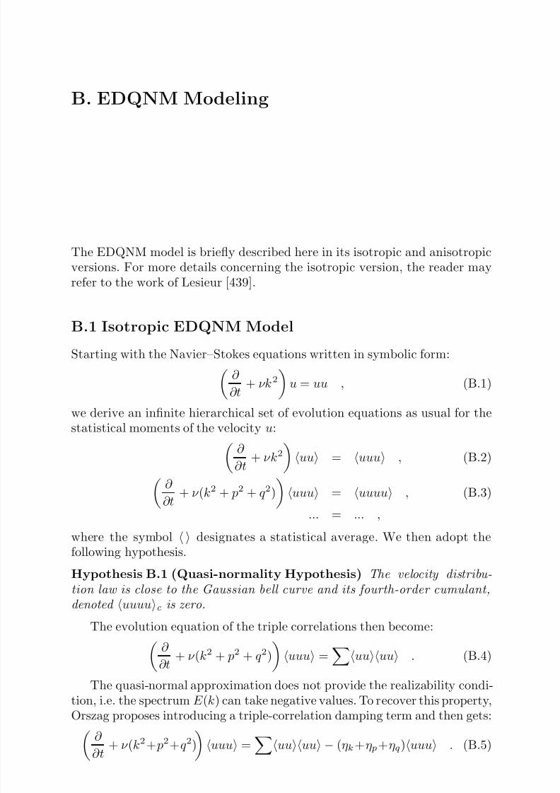
7/21/2019 Large Eddy Simulation for Incompressible Flows
http://slidepdf.com/reader/full/large-eddy-simulation-for-incompressible-flows 524/573
B. EDQNM Modeling
The EDQNM model is briefly described here in its isotropic and anisotropicversions. For more details concerning the isotropic version, the reader may
refer to the work of Lesieur [439].
B.1 Isotropic EDQNM Model
Starting with the Navier–Stokes equations written in symbolic form:∂
∂t + νk2
u = uu , (B.1)
we derive an infinite hierarchical set of evolution equations as usual for thestatistical moments of the velocity u:∂
∂t + νk2
uu = uuu , (B.2)
∂
∂t + ν (k2 + p2 + q 2)
uuu = uuuu , (B.3)
... = ... ,
where the symbol designates a statistical average. We then adopt the
following hypothesis.Hypothesis B.1 (Quasi-normality Hypothesis) The velocity distribu-tion law is close to the Gaussian bell curve and its fourth-order cumulant,denoted uuuuc is zero.
The evolution equation of the triple correlations then become:∂
∂t + ν (k2 + p2 + q 2)
uuu =
uuuu . (B.4)
The quasi-normal approximation does not provide the realizability condi-
tion, i.e. the spectrum E (k) can take negative values. To recover this property,Orszag proposes introducing a triple-correlation damping term and then gets:
∂
∂t + ν (k2 + p2+q 2)
uuu =
uuuu − (ηk+η p+ηq)uuu . (B.5)

7/21/2019 Large Eddy Simulation for Incompressible Flows
http://slidepdf.com/reader/full/large-eddy-simulation-for-incompressible-flows 525/573
508 B. EDQNM Modeling
The solution to this equation is:
uuu(t) = t0 uuuue−(µk+µp+µq)t
dt , (B.6)
withµk = ηk + νk2 . (B.7)
To get a solution that is easier to calculate, we adopt the following hy-pothesis:
Hypothesis B.2 The relaxation time of the triple correlations is small com-pared with the relaxation time of the double correlations (which is also that
of the energy spectrum).
With this hypothesis, we can “Markovianize” equation (B.6), which leadsto:
uuu(t) =
uuuu t
0
e−(µk+µp+µq)tdt
=
uuuu1 − e−(µk+µp+µq)t
µk + µ p + µq. (B.8)
This relation closes the derivation equation of the second-order moments.This closure is equivalent to replacing the solution of the Navier–Stokes equa-tions with that of the following Langevin-type stochastic model:
∂
∂t + (ν + η(k, t))k2
u = f (k, t) , (B.9)
in which
η(k, t) = 1
2 Θkpq(t) p
kq
bkpqE (q, t)dpdq . (B.10)
The forcing term f is such that:
F (k, t) ≡ 4πk2
t0
f (k, t)f (k, s)|k|=csteds
=
Θkpq(t)
k3
pq akpqE ( p, t)E (q, t)dpdq , (B.11)
where akpq and bkpq are coefficients linked to the geometry of the triad
(k, p, q), defined as:
akpq = 1
2(1 − xyz − 2y2z2), bkpq =
p
k(xy + z3) , (B.12)
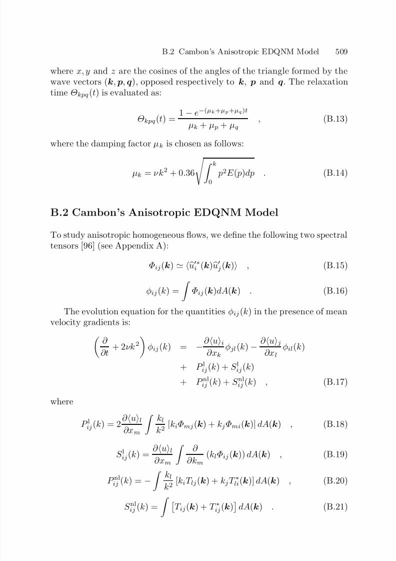
7/21/2019 Large Eddy Simulation for Incompressible Flows
http://slidepdf.com/reader/full/large-eddy-simulation-for-incompressible-flows 526/573
B.2 Cambon’s Anisotropic EDQNM Model 509
where x, y and z are the cosines of the angles of the triangle formed by thewave vectors (k, p, q), opposed respectively to k, p and q. The relaxationtime Θkpq(t) is evaluated as:
Θkpq(t) = 1 − e−(µk+µp+µq)t
µk + µ p + µq, (B.13)
where the damping factor µk is chosen as follows:
µk = νk2 + 0.36
k0
p2E ( p)dp . (B.14)
B.2 Cambon’s Anisotropic EDQNM Model
To study anisotropic homogeneous flows, we define the following two spectraltensors [96] (see Appendix A):
Φij(k) u∗i (k) uj(k) , (B.15)
φij(k) = Φij(k)dA(k) . (B.16)
The evolution equation for the quantities φij(k) in the presence of meanvelocity gradients is:
∂
∂t + 2νk2
φij(k) = −∂ ui
∂xkφjl(k) − ∂ uj
∂xlφil(k)
+ P lij(k) + S lij(k)
+ P nlij (k) + S nl
ij (k) , (B.17)
where
P lij(k) = 2∂ ul∂xm
kl
k2 [kiΦmj(k) + kjΦmi(k)] dA(k) , (B.18)
S lij(k) = ∂ ul
∂xm
∂
∂km(klΦij(k)) dA(k) , (B.19)
P nlij (k) = −
klk2
[kiT lj(k) + kjT ∗li(k)] dA(k) , (B.20)
S nlij (k) =
T ij(k) + T ∗ij(k)
dA(k) . (B.21)

7/21/2019 Large Eddy Simulation for Incompressible Flows
http://slidepdf.com/reader/full/large-eddy-simulation-for-incompressible-flows 527/573
510 B. EDQNM Modeling
Equation (B.17) is closed by replacing Φ(k) with a modeled form as a func-tion of φ(k), where the direction of k is controlled in the integrals (B.18)to (B.21):
P lij(k) = 2E (k)
2
5S ij
− 3D
S ljH li(k) + S liH lj(k) − 2
3δ ijS lmH lm(k)
+
14
3
D +
4
7
(Ω ilH lj(k) + Ω jlH li(k))
, (B.22)
S lij(k) = − 2
15S ij ∂
∂k (kE (k)) + 2S il ∂
∂k (kDE (k)H jl(k))
+ 2S jl ∂
∂k (kDE (k)H il(k))
− 1
3δ ijS lm ∂
∂k ([2 + 11D] kE (k)H lm(k)) , (B.23)
P nlij (k) = Θkpq
2
pq (x + yz)H ij(q )k1 pE ( p)E (q )y(z2
−y2)(a(q ) + 3)
+ (y + xz)a(q )
5
− p3E (k)E (q )y(z2 − x2)(a(q ) + 3)
dpdq , (B.24)
S nlij (k) =
Θkpq
2
pq
(xy + z3)
k2 pE ( p)E (q )
1
3δ ij + H ij( p)
+H ij(q )
− p3E (k)E (q )
1
3δ ij + H ij(k) + H ij(q )
+ H ij(q ) k2 pE ( p)E (q )ckpq − p3E (k)E (q )c pkq dpdq , (B.25)
where
S = 1
2
∇u + ∇T u , Ω = 1
2
∇u − ∇T u ,
and x, y and z are the cosines of the interior angles opposite the wave vec-tors k, p and q, respectively, in the triangle formed by these vectors. The
anisotropy parameter a(k) is optimized by the Rapid Distortion Theory. Thefactor D is defined as:
D = 2
7
1 +
4
5a
. (B.26)

7/21/2019 Large Eddy Simulation for Incompressible Flows
http://slidepdf.com/reader/full/large-eddy-simulation-for-incompressible-flows 528/573
B.3 EDQNM Model for Isotropic Passive Scalar 511
The energy and anisotropy spectra, denoted respectively E (k) and H ij(k),are given by the relations:
E (k) = 12
φll(k) , (B.27)
H ij(k) = φij(k)
2E (k) − 1
3δ ij . (B.28)
The geometric factor ckpq is defined as:
ckpq = 1
2(xy + z)
(y2 − z2)(a(q ) + 3) +
2
5a(q )(1 + z2)
. (B.29)
The relaxation time Θkpq(t) is evaluated as:
Θkpq(t) = 1 − e−(µk+µp+µq)t
µk + µ p + µq, (B.30)
where the damping term µk is:
µk = νk2 + 0, 36 k
0
p2E ( p)dp +
Ω
ij
Ω
ij
1/2
. (B.31)
It should be noted that fully anisotropic versions, which call for no angularparameter setting, have been proposed and compared with simulations for thecase of pure rotation and stable stratification [97].
B.3 EDQNM Model for Isotropic Passive Scalar
The transport equation for the passive scalar (15.1) can be rewritten in theFourier space under the following symbolic form:∂
∂t + κk2
θ = uθ , (B.32)
leading to a hierarchy of symbolic equtions for the statistical moments:
∂
∂t
+ κ(k2 + p2) uθ
=
θθu
, (B.33) ∂
∂t + [κ(k2 + p2) + νq 2]
θθu = θθuu , (B.34)
... = ... (B.35)
7/21/2019 Large Eddy Simulation for Incompressible Flows
http://slidepdf.com/reader/full/large-eddy-simulation-for-incompressible-flows 529/573
512 B. EDQNM Modeling
The EDQNM procedure can be applied to this set of equations to obtaina simple, closed equation for the temperature spectrum E θ(k). Details willnot be given here, since the process that yields the closed EDQNM modelinvolves the same steps as in the isotropic model for the velocity momentsdiscussed above. The reader can refer to Lesieur’s book [439] for a detailedpresentation. The model is expressed as
∂
∂t + 2κk2
E θ(k) =
Θθkpq
k
pq (1 − y2)E (q )[k2E θ( p) − p2E θ(k)]
× δ (k − p − q)dpdq , (B.36)
where the triad geometrical parameter is the same as in above sections, andthe characteristic time is defined as
Θθkpq = 1 − e−[κ(k2+ p2)+νq2+µ1(k)+µ1( p)+µ2(q)]t
κ(k2 + p2) + νq 2 + µ1(k) + µ1( p) + µ2(q ) , (B.37)
where
µi(k) = ai k
0
p2E ( p)dp, i = 1, 2 . (B.38)
The two constants a1 and a2 are not uniquely defined, and several choicesare possible. Setting a1 = 0 and a2 = 1.3 enables the solve analytically thesystem and yields a satisfactory prediction from a physical point of view.
Another possibility is to take a1 = a2 = 0.218K 3/20 .
Anisotropic passive scalar models [303] and models for stably stratifiedflows [266, 689, 267] are very complex and will not be discussed here. This isalso the case of EDQNM models for mixed scalars [723].
7/21/2019 Large Eddy Simulation for Incompressible Flows
http://slidepdf.com/reader/full/large-eddy-simulation-for-incompressible-flows 530/573
References
1. Abba, A., Bucci, R., Cercignani, C., Valdettaro, L. (1996): A new approachto the dynamic subgrid scale model. Unpublished
2. Adams, N. (2001): The role of deconvolution and numerical discretizationin subgrid-scale modeling. (Direct and large-eddy simulation IV, Geurts,Friedrich and Metais eds.), Kluwer, 311–320
3. Adams, N.A., Leonard, A. (1999): Deconvolution of subgrid-scales for thesimulation of shock-turbulence interaction. (Direct and Large Eddy SimulationIII, Voke, Sandham and Kleiser eds.) Kluwer, 201–212
4. Adams, N.A., Stolz, S. (2001): Deconvolution methods for subgrid-scale ap-proximation in LES. (Modern simulation strategies for turbulent flow, Geurtsed.), Edwards, 21–44
5. Addad, Y., Laurence, D., Talotte, C., Jacob, M.C. (2003): Large eddy simu-lation of a forward facing step for acoustic source identification. Int. J. Heat
Fluid Flow 24, 562–5716. Adrian, J. (1990): Stochastic estimation of subgrid-scale motions. Appl. Mech.Rev. 43(5), 214–218
7. Agee, E., Gluhovsky, A. (1999): LES model sensitivities to domains, grids,and large-eddy timescales. J. Atmos. Sci. 56, 599–604
8. Akhavan, R., Ansari, A., Kang, S., Mangiavacchi, N. (2000): Subgrid-scaleinteractions in a numerically simulated planar turbulent jet an implicationsfor modelling. J. Fluid Mech. 408, 83–120
9. Akselvoll, K., Moin, P. (1996): Large-eddy simulation of turbulent confinedcoannular jets. J. Fluid Mech. 315, 387–411
10. Allen, R., Mendonca, F. (2004): DES validations of cavity acoustics over the
subsonic to supersonic range. AIAA Paper 2004-286211. Alvelius, K., Johansson, A. (2000): LES computations and comparison withKolmogorov theory for two-point pressure-velocity correlations and structurefunctions for globally anisotropic turbulence. J. Fluid Mech. 403, 23–36
12. Anderson, R., Meneveau, C. (1999): Effects of the similarity model in finite-difference LES of isotropic turbulence using a Lagrangian dynamic mixedmodel. Flow, Turbulence and Combustion 62, 201–225
13. Anitescu, M., Layton, W. (2002): Uncertainties in large-eddy simulation andimproved estimates of turbulent flow functionals. Unpublished
14. Antonopoulos-Domis, M. (1981): Aspects of large-eddy simulation of homo-geneous isotropic turbulence. Int. J. Numer. Meth. Fluids 1, 273–290
15. Aprovitola, A., Denaro, F. (2004): On the application of congruent upwinddiscretizations for large eddy simulations. J. Comput. Phys. 194, 329–34316. Arad, E. (2001): Analysis of boundary layer separation over a bump using
large-eddy simulation. AIAA Paper 2001-2558
7/21/2019 Large Eddy Simulation for Incompressible Flows
http://slidepdf.com/reader/full/large-eddy-simulation-for-incompressible-flows 531/573
514 References
17. Arandiga, F., Donat, R., Harten, A. (1999): Multiresolution based on weightedaverages of the hat function II: nonlinear reconstruction techniques. SIAM J.Sci. Comput. 20(3), 1053–1093
18. Armenio, V., Piomelli, U. (2000): A Lagrangian mixed subgrid-scale model ingeneralized coordinates. Flow, Turbulence and Combustion 65, 51–81
19. Armenio, V., Sarkar, S. (2002): An investigation of stably stratified turbulentchannel flow using large-eddy simulation. J. Fluid Mech. 459, 1–42
20. Arunajatesan, S., Sinha, N. (2000): Towards hybrid LES-RANS computationsof cavity flowfileds. AIAA Paper 2000-0401
21. Arunajatesan, S., Sinha, N. (2001): Unified unsteady RANS-LES simulationsof cavity flowfields. AIAA Paper 2001-0516
22. Arunajatesan, S., Sinha, N., Ukeiley, L. (2001): On the application of hybridRANS-LES and Proper Orthogonal Decomposition techniques to control of cavity flows. (DNS/LES Progress and Challenges, Liu, Sakell and Beutner
eds.), Greyden Press, 673–68823. Aupoix, B. (1984): Eddy viscosity subgrid models for homogeneous turbu-
lence. (Proceedings of “Macroscopic modelling of turbulent flows”, Lecturenotes in physics, Vol. 230), Springer-Verlag, 45–64
24. Aupoix, B. (1985): Subgrid scale models for homogeneous anisotropic tur-bulence. (Proceedings of the Euromech Colloquium 199, “Direct and largeeddy simulation of turbulence”, Notes on numerical fluid mechanics, Vol. 15)Vieweg, 36–66
25. Aupoix, B. (1989): Application of two-point closures to subgrid scale modellingfor homogeneous 3D turbulence. (Turbulent shear flows, von Karman Institutefor Fluid Dynamics, Lecture Series 1989-03)
26. Aupoix, B., Cousteix, J. (1982): Modeles simples de tensions de sous-mailleen turbulence homogene isotrope (in french). Rech. Aero. 4, 273–283
27. Avancha, R., Pletcher, R. (2002): Large eddy simulation of the flow pasta backward facing step with heat transfer and property variations. Int. J.Heat Fluid Flow 23, 601–614
28. Baastians, R., Rindt, C., Nieuwstadt, F., van Steenhoven, A. (2000): Directand large-eddy simulation of the transition of two- and three-dimensionalplane plumes in a confined enclosure. Int. J. Heat Mass Transfer 43, 2375–2393
29. Baastians, R., Rindt, C., van Steenhoven, A. (1998): Experimental analysis of a confined transitional plume with respect to subgrid-scale modeling. Int. J.Heat Mass Transfer 41, 3989–4007
30. Bagget, J.S. (1997): Some modeling requirements for wall models in large-eddy simulation. Annual Research Briefs – Center for Turbulence Research,123–134
31. Bagget, J.S. (1998): On the feasability of merging LES with RANS for thenear-wall region of attached turbulent flows. Annual Research Briefs – Centerfor Turbulence Research, 267–277
32. Bagget, J.S., Jimenez, J., Kravchenko, A.G. (1997): Resolution requirementsin large-eddy simulations of shear flows. Annual Research Briefs – Center forTurbulence Research, 51–66
33. Bagget, J.S., Nicoud, F., Mohammadi, B., Bewley, T., Gullbrand, J., Bo-tella, O. (2000): Sub-optimal control based wall models for LES including
transpiration velocity. Proceedings of the Summer Program – Center for Tur-bulence Research, 331–342
34. Bagwell, T.G., Adrian, R.J., Moser, R.D., Kim, J. (1993): Improved approx-imation of wall shear stress boundary conditions for large-eddy simulation.(Near-wall turbulent flows, So, Speziale and Launder eds.), Elsevier

7/21/2019 Large Eddy Simulation for Incompressible Flows
http://slidepdf.com/reader/full/large-eddy-simulation-for-incompressible-flows 532/573
References 515
35. Balaras, E. (2003): Modeling complex boundaries using an external force fieldon fixed Cartesian grids in large-eddy simulations. Computers and Fluids 33,375–404
36. Balaras, E., Benocci, C., Piomelli, U. (1995): Finite-difference computations of high Reynolds number flows using the dynamic subgrid-scale model. Theoret.Comput. Fluid Dynamics 7, 207–216
37. Balaras, E., Benocci, C., Piomelli, U. (1996): Two-layer approximate boundaryconditions for large-eddy simulations. AIAA Journal 34(6), 1111–1119
38. Balaras, E., Piomelli, U., Wallace, J.M. (2001): Self-similar states in turbulentmixing layers. J. Fluid Mech. 446, 1–24
39. Bardina, J., Ferziger, J.H., Reynolds, W.C. (1980): Improved subgrid scalemodels for large eddy simulation. AIAA Paper 80-1357
40. Bardina, J., Ferziger, J.H., Reynolds, W.C. (1983): Improved turbulence mo-dels based on large eddy simulation of homogeneous, incompressible, turbulent
flows. Report TF-19, Thermosciences Division, Dept. Mechanical Engineering,Stanford University
41. Barenblatt, G.I. (1996): Scaling, self-similarity, and intermediate asymptotics.Cambridge University Press, UK
42. Basdevant, C., Lesieur, M., Sadourny, R. (1978): Subgrid-scale modeling of en-strophy transfer in two-dimensional turbulence. J. Atmos. Sci. 35, 1028–1042
43. Basdevant, C., Sadourny, R. (1983): Modelisation des echelles virtuelles dansla modelisation numerique des ecoulements turbulents bidimensionnels (infrench). J. Mech. Theor. Appl., numero special, 243–269
44. Bastin, F., Lafon, P., Candel, S. (1997): Computation of jet mixing noise dueto coherent structures: the plane jet case. J. Fluid Mech. 335, 261–304
45. Batchelor, G.K. (1953): The theory of homogeneous turbulence. CambridgeUniversity Press
46. Batten, P., Goldberg, U., Chakravarthy, S. (2000): Sub-grid turbulence moel-ing for unsteady flow with acoustic resonance. AIAA Paper 2000-0473
47. Batten, P., Goldberg, U., Chakravarthy, S. (2002): Reconstructed subgridmethods for acoustics predictions at all Reynolds numbers. AIAA Paper 2002-2511
48. Batten, P., Goldberg, U., Chakravarthy, S. (2003): Using synthetic turbulenceto interface RANS and LES. AIAA Paper 2003-0081
49. Batten, P., Goldberg, U., Chakravarthy, S. (2004): Interfacing statistical tur-bulence closures with large-eddy simulation. AIAA Journal 42(3), 485–492
50. Baurle, R.A., Tam, C.J., Edwards, J.R., Hassan, H.A. (2003): Hybrid simula-tion approach for cavity flows: blending, algorithm, and boundary treatmentissues. AIAA Journal 41(8), 1463–1480
51. Beaubert, F., Viazzo, S. (2003): Large eddy simulations of plane turbulentimpinging jets at moderate Reynolds numbers. Int. J. Heat Fluid Flow 24,512–519
52. Beaudan, P., Moin, P. (1994): Numerical experiments on the flow past a cir-cular cylinder at subcritical Reynolds number. Report TF-62, ThermosciencesDivision, Dept. Mechanical Engineering, Stanford University
53. Benzi, R., Biferale, L., Succi, S., Toschi, F. (1999): Intermittency and eddyviscosities in dynamical models of turbulence. Phys. Fluids 11(5), 1221–1228
54. Berkooz, G. (1994): An observation on probability density equations, or, whendo simulations reproduce statistics? Nonlinearity 7, 313–328
55. Berkooz, G., Holmes, P., Lumley, J.L. (1993): The proper othogonal decom-position in the analysis of turbulent flows. Ann. Rev. Fluid Mech. 25, 539–575

7/21/2019 Large Eddy Simulation for Incompressible Flows
http://slidepdf.com/reader/full/large-eddy-simulation-for-incompressible-flows 533/573
516 References
56. Bertoglio, J.P. (1984): A stochastic subgrid model for sheared turbulence.(Proceedings of Macroscopic modelling of turbulent flows, Lecture notes inphysics, Vol. 230) Springer-Verlag, 100–119
57. Bertoglio, J.P., Mathieu, J. (1984): A stochastic subgrid model for large-eddysimulation: general formulation. C. R. Acad. Sc. Paris 299, serie II, (12),751–754
58. Bertoglio, J.P., Mathieu, J. (1984): A stochastic subgrid model for large-eddysimulation: generation of a stochastic process. C. R. Acad. Sc. Paris 299, serieII, (13), 835–838
59. Biringen, S., Reynolds, W.C. (1981): Large-eddy simulation of the shear-freeturbulent boundary-layer. J. Fluid Mech. 103, 53–63
60. Blackburn, H., Schmidt, S. (2003): Spectral element filtering techniques forlarge eddy simulation with dynamic estimation. J. Comput. Phys. 186, 610–629
61. Blin, L., Hadjadj, A., Vervisch, L. (2003): Large eddy simulation of turbulentflows in reversing systems. JOT, 1–19
62. Boersma, B.J., Kooper, M.N., Nieuwstadt, F.T.M., Wesseling, P. (1997): Localgrid refinement in large-eddy simulation. J. Engng. Math.32, 161–175
63. Bogey, C., Bailly, C. (2004): A family of low dispersive and low dissipativeexplicit schemes for flow and noise computations. J. Comput. Phys. 194, 194–214
64. Bonnet, J.P., Delville, J., Druault, P., Sagaut, P., Grohens, R. (1997): Lin-ear stochastic estimation of LES inflow conditions. (Advances in DNS/LES,C. Liu, Z. Liu (eds.)) Greyden Press, 341–348
65. Booij, R. (2003): Measurements and large eddy simulations of the flows in
some curved flumes. JOT 4, 1–1766. Boris, J.P., Book, D.L. (1973): Flux-Corrected Transport. I. SHASTA, a fluid
transport algorithm that works. J. Comput. Phys. 11, 38–6967. Boris, J.P., Grinstein, F.F., Oran, E.S., Kolbe, R.L. (1992): New insights into
large-eddy simulation. Fluid Dyn. Res. 10, 199–22868. Borue, V., Orszag, S.A. (1995): Forced three-dimensional homogeneous tur-
bulence with hyperviscosity. Europhys. Lett. 29, 687–69269. Borue, V., Orszag, S.A. (1995): Self-similar decay of three-dimensional turbu-
lence with hyperviscosity. Phys. Rev. E. 52, R856–85970. Borue, V., Orszag, S.A. (1996): Numerical study of Kolmogorov flow at high
Reynolds numbers. J. Fluid Mech. 306, 293–323
71. Borue, V., Orszag, S.A. (1996): Kolmogorov’s refined similarity hypothesis forhyperviscous turbulence. Phys. Rev. E. 366, R21–24
72. Borue, V., Orszag, S.A. (1998): Local energy flux and subgrid-scale statisticsin three-dimensional turbulence. J. Fluid Mech. 366, 1–31
73. Bouchon, F., Dubois, T. (1999): Incremental Unknowns: a tool for large-eddysimulations ?. (Direct and Large Eddy Simulation III, Voke, Sandham andKleiser eds) Kluwer, 275–286
74. Brasseur, J.G., Wei, C.H. (1994): Interscale dynamics and local isotropy inhigh Reynolds number turbulence within triadic interactions. Phys. Fluids A6(2), 842–870
75. Breuer, M. (1998): Large eddy simulation of the subcritical flow past a circular
cylinder: numerical and modeling aspects. Int. J. Numer. Meth. Fluids 28,1281–1302
76. Breuer, M. (1998): Numerical and modeling influences on large eddy simula-tions for the flow past a circular cylinder. Int. J. Heat Fluid Flow 19, 512–521
77. Breuer, M. (2000): A challenging test case for large eddy simulation: highReynolds number circular cylinder flow. Int. J. Heat Fluid Flow 21, 648–654
7/21/2019 Large Eddy Simulation for Incompressible Flows
http://slidepdf.com/reader/full/large-eddy-simulation-for-incompressible-flows 534/573
References 517
78. Breuer, M., Jovicic, N., Mazaev, K. (2003): Comparison of DES, RANS andLES for the separated flow around a flat plate at high incidence. Int. J. Numer.Meth. Fluids 41, 357–388
79. Brezzi, F., Houston, P., Marini, D., Suli, E. (2000): Modeling subgrid viscosityfor advection-diffusion problems. Comput. Methods Appl. Mech. Engrg. 190,1601–1610
80. Brown, R.M., Perry, P., Shen, Z. (1998): The additive turbulent decompositionfor the two-dimensional incompressible Navier–Stokes equations: convergencetheorems and error estimates. SIAM J. Appl. Math. 59(1), 139–155
81. Brun, C., Friedrich, R. (2001): Modeling the test SGS tensor T ij : an issue inthe dynamic approach. Phys. Fluids 13(8), 2373–2385
82. Brun, C., Friedrich, R. (2001): The spatial velocity increment as a tool forSGS modeling. (Modern simulation strategies for turbulent flow, Geurts (ed.)),Edwards, 57–84
83. Brun, C., Kessler, P., Comte, P., Lesieur, M. (1997): Simulation des grandesechelles de jets ronds (in french). Rapport de synthese, Contrat DGA/DRET95-2557 A
84. Bush, R.H., Mani, M. (2001): A two-equation large eddy stress model for highsubgrid shear. AIAA Paper 2001-2561
85. Cabot, W. (1992): Large eddy simulations of time-dependent and buoyancy-driven channel flows. Annual Research Briefs – Center for Turbulence Re-search, 45–60
86. Cabot, W. (1995): Large-eddy simulations with wall models. Annual ResearchBriefs – Center for Turbulence Research, 41–49
87. Cabot, W. (1996): Near-wall models in large-eddy simulations of flow behind
a backward-facing step. Annual Research Briefs – Center for Turbulence Re-search, 199–210
88. Cabot, W. (1998): Large-eddy simulation of a separated boundary layer. An-nual Research Briefs – Center for Turbulence Research, 279–288
89. Cabot, W., Jimenez, J., Bagget, J.S. (1999): On wakes and near-wall be-havior in coarse large-eddy simulation of channel flow with wall models andsecond-order finite-difference methods. Annual Research Briefs – Center forTurbulence Research, 343–354
90. Cabot, W., Moin, P. (1999): Approximate wall boundary conditions in thelarge-eddy simulation of high Reynolds number flow. Flow, Turbulence andCombustion 63, 269–291
91. Calgaro, C., Debussche, A., Laminie, J. (1998): On a multilevel approachfor the two-dimensional Navier–Stokes equations with finite elements. Int. J.Numer. Meth. Fluids 27, 241–258
92. Calmet, I., Magnaudet, J. (1997): Large-eddy simulation of high-Schmidtnumber mass transfer in a turbulent channel flow. Phys. Fluids 9(2), 438–455
93. Calmet, I., Magnaudet, J. (1998): High-Schmidt number mass transfer throughturbulent gas-liquid interfaces. Int. J. Heat Fluid Flow 19, 522–532
94. Camarri, S., Salvetti, M., Koobus, B., Dervieux, A. (2002): Large-eddy simu-lation of a bluff-body flow on unstructurd grids. Int. J. Numer. Meth. Fluids40, 1431–1460
95. Camarri, S., Salvetti, M., Koobus, B., Dervieux, A. (2004): A low-diffusion
MUSCL scheme for LES on unstructured grids. Computers and Fluids 33,1101–1129
96. Cambon, C., Jeandel, D., Mathieu, J. (1981): Spectral modelling of homoge-neous non-isotropic turbulence. J. Fluid Mech. 104, 247–262
97. Cambon, C., Mansour, N.N., Godeferd, F.S. (1997): Energy transfer in rotat-ing turbulence. J. Fluid Mech. 337, 303–332

7/21/2019 Large Eddy Simulation for Incompressible Flows
http://slidepdf.com/reader/full/large-eddy-simulation-for-incompressible-flows 535/573
518 References
98. Cantekin, M.E., Westerink, J.J., Luettich, R.A. (1994): Low and moderateReynolds number transient flow simulations using space filtered Navier–Stokesequations. Numer. Meth. Partial Diff. Eq. 10, 491–524
99. Canuto, V.M., Cheng, Y. (1997): Determination of the Smagorinsky-Lilly con-stant C S. Phys. Fluids 9(5), 1368–1378
100. Carati, D., Cabot, W. (1996): Anisotropic eddy viscosity models. Proceedingsof the Summer Program – Center for Turbulence Research, 249–259
101. Carati, D., Ghosal, S., Moin, P. (1995): On the representation of backscatterin dynamic localization models. Phys. Fluids 7(3), 606–616
102. Carati, D., Rogers, M.M. (1998): Ensemble-averaged LES of time-evolvingplane wake. Proceedings of the Summer Program – Center for TurbulenceResearch, 325–336
103. Carati, D., Rogers, M., Wray, A. (2002): Statistical ensemble of large-eddysimulations. J. Fluid Mech. 455, 195–212
104. Carati, D., Vanden Eijnden, E. (1997): On the self-similarity assumption indynamic models for large-eddy simulations. Phys. Fluids 9 (7), 2165–2167
105. Carati, D., Winckelmans, G.S., Jeanmart, H. (1999): Exact expansions forfiltered-scales modelling with a wide class of LES filters. (Direct and LargeEddy Simulation III, Voke, Sandham and Kleiser eds) Kluwer, 213–224
106. Carati, D., Winckelmans, G., Jeanmart, H. (2001): On the modelling of thesubgrid-scale and filtered-scale stress tensors in large-eddy simulation. J. FluidMech. 441, 119–138
107. Carati, D., Wray, A. (2000): Time filtering in large-eddy simulations. Proceed-ings of the Summer Program – Center for Turbulence Research, 263–270
108. Carati, D., Wray, A., Cabot, W. (1996): Ensemble-averaged dynamic model-
ing. Proceedings of the Summer Program – Center for Turbulence Research,237–248
109. Carlotti, P. (2002): Two-point properties of atmospheric turbulence very closeto the ground: comparison of a high resolution LES with theoretical models.Boundary-Layer Meteorol. 104, 381–410
110. Carnevale, G., Briscolini, M., Orlandi, P. (2001): Buoyancy- to inertial-rangetransition in forced stratified turbulence. J. Fluid Mech. 427, 205–239
111. Carruthers, D.J., Moeng, C.H. (1987): Waves in the overlying inversion of theconvective boundary layer. J. Atmos. Sci. 44(4), 1801–1808
112. Casalino, D., Boudet, J., Jacob, M.: A shear flow subgrid scale model for largeeddy simulations. Submitted
113. Catalano, P., Wang, M., Iaccarino, G., Moin, P. (2003): Numerical simulationof the flow around a circular cylinder at high Reynolds numbers. Int. J. HeatFluid Flow 24, 463–469
114. Cerutti, S., Meneveau, C. (1998): Intermittency and relative scaling of subgrid-scale energy dissipation in isotropic turbulence. Phys. Fluids 10 (4), 928–937
115. Cerutti, S., Meneveau, C., Knio, O.M. (2000): Spectral and hyper eddy vis-cosity in high-Reynolds-number turbulence. J. Fluid Mech. 421, 307–338
116. Cerutti, S., Meneveau, C. (2000): Statistics of filtered velocity in grid andwake turbulence. Phys. Fluids 12(5), 1143–1165
117. Chakravarthy, V.K., Menon, S. (2001): Large-eddy simulation of turbulentpremixed flames in the flamelet regime. Combust. Sci. and Tech. 162, 175–
222118. Chakravarthy, V.K., Menon, S. (2001): Subgrid modeling of turbulent pre-
mixed flames in the flamelet regime. Flow, Turbulence and Combustion 65,133–161
119. Chapman, D.R. (1979): Computational aerodynamics development and out-look. AIAA Journal 17(12), 1293–1313
7/21/2019 Large Eddy Simulation for Incompressible Flows
http://slidepdf.com/reader/full/large-eddy-simulation-for-incompressible-flows 536/573
References 519
120. Chasnov, J.R. (1990): Simulation of the Kolmogorov inertial subrange usingan improved subgrid model. Phys. Fluids A 3(1), 188–200
121. Chasnov, J. (1991): Simulation of the inertial-conductive subrange. Phys. Flu-
ids A 3(5), 1164–1168122. Chasnov, J. (1994): Similarity states of passive scalar transport in isotropic
turbulence. Phys. Fluids 6(2), 1036–1051123. Chasnov, J. (1995): Similarity states of passive scalar transport in buoyancy-
generated turbulence. Phys. Fluids 7(6), 1499–1506124. Chasnov, J., Tse, K.L. (2001): Turbulent penetrative convection with an in-
ternal heat source. Fluid Dyn. Res. 28, 397–421125. Chatelain, A., Ducros, F., Metais, O. (2004): LES of turbulent heat trans-
fer: proper convection numerical schemes for temperature transport. Int. J.Numer. Meth. Fluids 44, 1017–1044
126. Chattopadhyay, H., Saha, S. (2003): Turbulent flow and heat transfer from
a slot jet impinging on a moving plate. Int. J. Heat Fluid Flow 24, 685–697127. Chen, S., Doolen, G.D. (1998): Lattice Boltzmann method for fluid flows. Ann.
Rev. Fluid Mech. 30, 329–364128. Chen, M., Temam, R. (1991): Incremental unknowns for solving partial dif-
ferential equations. Numer. Math. 59, 255–271129. Chester, S., Charlette, F., Meneveau, C. (2001): Dynamic model for LES with-
out test filtering: quantifying the accuracy of Taylor series approximations.Theoret. Comput. Fluid Dynamics 15, 165–181
130. Chlond, A. (1998): Large-eddy simulation of contrails. J. Atmos. Sci. 55, 796–819
131. Choi, H., Moin, P. (1994): Effects of the computational time step on numerical
solutions of turbulent flow. J. Comput. Phys. 113, 1–4132. Chollet, J.P. (1983): Two-point closures as a subgrid modelling for large-eddy
simulations. (Fourth Symposium on Turbulent Shear Flows, Karlsruhe, Alle-magne)
133. Chollet, J.P. (1984): Spectral closures to derive a subgrid scale modelling forlarge eddy simulation. (Proceedings of Macroscopic modelling of turbulentflows, Lecture notes in physics, Vol. 230), Springer-Verlag, 161–176
134. Chollet, J.P. (1984): Turbulence tridimensionnelle isotrope: modelisationstatistique des petites echelles et simulation numerique des grandes echelles(in french). These de Doctorat es-sciences, Grenoble, France
135. Chollet, J.P. (1992): LES and subgrid models for reactive flows and combus-
tion. ERCOFTAC Summer School/Workshop on modelling turbulent flows,Lyon, France
136. Chollet, J.P., Lesieur, M. (1981): Parametrization of small scales of three-dimensional isotropic turbulence utilizing spectral closures. J. Atmos. Sci. 38,2747–2757
137. Chorin, A., Kast, A., Kupferman, R. (1998): Optimal prediction of under-resolved dynamics. Proc. Natl. Acad. Sci. USA, Applied Mathematics 95,4094–4098
138. Chow, F.K., Moin, P. (2003): A further study of numerical errors in large-eddysimulations. J. Comput. Phys. 184, 366–380
139. Chung, Y.M., Sung, H.J. (1997): Comparative study of inflow conditions for
spatially evolving simulation. AIAA Journal 35(2), 269–274140. Chyczewski, T., Morris, P., Long, L. (2000): Large-eddy simulation of
wall bounded flow using the nonlinear disturbance equations. AIAA Paper2000-2007
141. Ciofalo, M. (1996): Investigation of flow and heat transfer in corrugated pas-sages–II. Numerical simulations. Int. J. Heat Mass Transfer 39(1), 165–192

7/21/2019 Large Eddy Simulation for Incompressible Flows
http://slidepdf.com/reader/full/large-eddy-simulation-for-incompressible-flows 537/573
520 References
142. Ciofalo, M., Collins, M.W. (1992): Large-eddy simulation of a turbulent flowand heat transfer in plane and rib-roughened channels. Int. J. Numer. Meth.Fluids 15, 453–489
143. Clark, R.A., Ferziger, J.H., Reynolds, W.C. (1979): Evaluation of subgrid-scalemodels using an accurately simulated turbulent flow. J. Fluid Mech. 91(1),1–16
144. Codina, R. (2000): Stabilization of incompressibility and convection throughorthogonal sub-scales in finite elements methods. Comput. Methods Appl.Mech. Engrg. 190, 1579–1599
145. Colella, P., Woodward, P.R. (1984): The Piecewise Parabolic Method (PPM)for gas-dynamical simulations. J. Comput. Phys. 54, 174–201
146. Constantinescu, G.S., Squires, K.D. (2000): LES and DES investigations of turbulent flow over a sphere. AIAA Paper 2000-0540
147. Conway, S., Caraeni, D., Fuchs, L. (2000): Large eddy simulation of the flow
through the blade of a swirl generator. Int. J. Heat Fluid Flow 21, 664–673148. Cook, A.W. (1997): Determination of the constant coefficient in the scale si-
milarity models of turbulence. Phys. Fluids 9(5), 1485–1487149. Cook, A. (2001): A consistent approach to large-eddy simulation using adap-
tive mesh refinement. J. Comput. Phys. 154, 117–133150. Cousteix, J. (1989): Turbulence et couche limite (in french). CEPADUES –
Editions, France151. Cui, J., Patel, V., Lin, C.L. (2003): Large eddy simulation of turbulent flow
in a channel with rib roughness. Int. J. Heat Fluid Flow 24, 372–388152. Cui, A., Street, R.L. (2001): Large-eddy simulation of turbulent rotating con-
vective flow development. J. Fluid Mech. 447, 53–84
153. Cui, G., Zhou, H., Zhang, Z., Shao, L. (2004): A new dynamic subgrid eddyviscosity model with application to turbulent channel flow. Phys. Fluids 16(8),2835–2842
154. Cuxart, J., Bougeault, P., Redelsperger, J.L. (2000): A turbulence schemeallowing for mesoscale and large-eddy simulations. Q.J.R. Meteorol. Soc. 126,1–30
155. Cziesla, T., Biswas, G., Chattopadhyay, H., Mitra, N. (2001): Large eddysimulation of flow and heat transfer in an impinging slot jet. Int. J. HeatFluid Flow 22, 500-508
156. Cziesla, T., Biswas, G., Mitra, N.K. (1999): Large eddy simulation in a turbu-lent channel flow using exit boundary conditions. Int. J. Numer. Meth. Fluids
30, 763–773157. da Silva, C., Metais, O. (2002): Vortex control of bifurcating jets: a numerical
study. Phys. Fluids 14(11), 3798–3818158. da Silva, C., Metais, O. (2002): On the influence of coherent structures upon
interscale interactions in turbulent plane jets. J. Fluid Mech. 473, 103–145159. Dai, Y., Kobayashi, T., Taniguchi, N. (1994): Large eddy simulation of plane
turbulent jet flow using a new outflow velocity boundary condition. JSMEInternational Journal Series B 37(2), 242–253
160. Dakhoul, Y.M., Bedford, K.W. (1986): Improved averaging method for tur-bulent flow simulation. Part 1: theoretical development and application toBurger’s transport equation. Int. J. Numer. Meth. Fluids 6, 49–64
161. Dakhoul, Y.M., Bedford, K.W. (1986): Improved averaging method for tur-bulent flow simulation. Part 2: calculations and verification. Int. J. Numer.Meth. Fluids 6, 65–82
162. Dang, K.T. (1985): Evaluation of simple subgrid-scale models for the numer-ical simulation of homogeneous turbulence. AIAA Journal 23(2), 221–227

7/21/2019 Large Eddy Simulation for Incompressible Flows
http://slidepdf.com/reader/full/large-eddy-simulation-for-incompressible-flows 538/573
References 521
163. Dantinne, G., Jeanmart, H., Winckelmans, G.S., Legat, V. (1998): Hypervis-cosity and vorticity-based models for subgrid scale modeling. Applied Scien-tific Research 59, 409–420
164. Das, A., Moser, R.D. (2001): Filtering boundary conditions for LES and em-bedded boundary simulations. (DNS/LES Progress and Challenges, Liu, Sakelland Beutner eds.), Greyden Press, 389–396
165. Das, A., Moser, R. (2002): Optimal large-eddy simulation of forced burgersequation. Phys. Fluids 14(12), 4344–4351
166. David, E. (1993): Modelisation des ecoulements compressibles et hyperson-iques (in french). These de Doctorat de l’INPG, Grenoble, France
167. Davidson, L. (2001): Hybrid LES-RANS: a combination of a one-equationSGS model and a K –ω model for predicting recirculating flows. (Proceedingsof ECCOMAS CFD conference)
168. de Bruyn Kops, S., Riley, J. (2000): Re-examining the thermal mixing layer
with numerical simulations. Phys. Fluids. 12(1), 185–192169. De Stefano, G., Denaro, F.M., Riccardi, G. (1998): Analysis of 3D backward-
facing step incompressible flows via a local averaged-based numerical proce-dure. Int. J. Numer. Meth. Fluids 28, 1073–1091
170. De Stefano, G., Denaro, F.M., Riccardi, G. (2001): High-order filtering forcontrol volumes flow simulation. Int. J. Numer. Meth. Fluids 37(7), 797–835
171. De Stefano, G., Vasilyev, O.V. (2002): Sharp cutoff versus smooth filtering inlarge eddy simulation. Phys. Fluids 14(1), 362–369
172. Deardorff, J.W. (1970): A numerical study of three-dimensional turbulentchannel flow at large Reynolds numbers. J. Fluid Mech. 41, 453–465
173. Deardorff, J.W. (1973): The use of subgrid transport equations in a three-
dimensional model of atmospheric turbulence. ASME J. Fluids Engng.,429–438
174. Debussche, A., Dubois, T., Temam, R. (1995): The nonlinear Galerkinmethod: a multiscale method applied to simulation of homogeneous turbu-lent flows. Theoret. Comp. Fluid Dynamics 7, 279–315
175. Denaro, F.M. (1996): Towards a new model-free simulation of high-Reynolds-number flows: local average direct numerical simulation. Int. J. Numer. Meth-ods Fluids 23, 125–142
176. Deschamps, V. (1988): Simulation numerique de la turbulence homogene in-compressible dans un ecoulement de canal plan (in french). ONERA, Notetechnique 1988-5
177. Desjardin, P.E., Frankel, S.H. (1996): Assessment of turbulent combustionsubmodels using the linear eddy model. Combust. Flame 104, 343–357
178. di Mare, L., Jones, W.P. (2003): LES of turbulent flow past a swept fence.Int. J. Heat Fluid Flow 24, 606–615
179. Ding, X., Tsang, T.T.H. (2001): Large eddy simulation of turbulent flows bya least-squares finite element method. Int. J. Numer. Meth. Fluids 37, 297–319
180. Diurno, G.V., Balaras, E., Piomelli, U. (2001): Wall-layer models for LES of separated flows. (Modern simulation strategies for turbulent flow, Geurts ed.),Edwards, 207–222
181. Domaradzki, J.A., Adams, N.A. (2002): Direct modelling of subgrid scales of turbulence in large eddy simulations. JOT 3(024), 1–19
182. Domaradzki, J.A., Holm, D.D. (2001): The Navier–Stokes-alpha model: LESequations with nonlinear dispersion. (Modern simulation strategies for turbu-lent flow, Geurts ed.), Edwards, 107–122
183. Domaradzki, J.A., Horiuti, K. (2001): Similarity modeling on an expandedmesh applied to rotating turbulence. Phys. Fluids 13(11), 3510–3512

7/21/2019 Large Eddy Simulation for Incompressible Flows
http://slidepdf.com/reader/full/large-eddy-simulation-for-incompressible-flows 539/573
522 References
184. Domaradzki, J.A., Liu, W. (1995): Approximation of subgrid-scale energytransfer based on the dynamics of the resolved scales of turbulence. Phys.Fluids 7(8), 2025–2035
185. Domaradzki, J.A., Liu, W., Brachet, M.E. (1993): An analysis of subgrid-scaleinteractions in numerically simulated isotropic turbulence. Phys. Fluids 5(7),1747–1759
186. Domaradzki, J.A., Liu, W., Hartel, C., Kleiser, L. (1994): Energy transfer innumerically simulated wall-bounded turbulent flows. Phys. Fluids 6(4), 1583–1599
187. Domaradzki, J.A., Loh, K.C. (1999): The subgrid-scale estimation model inthe physical space representation. Phys. Fluids 11 (8), 2330–2342
188. Domaradzki, J.A., Loh, K.C. (2002): Large eddy simulations using the subgrid-scale estimation model and truncated Navier–Stokes dynamics. Theoret. Com-put. Fluid Dynamics 15, 421–450
189. Domaradzki, J.A., Metcalfe, R.W., Rogallo, R.S., Riley, J.J. (1987): Analysisof subgrid-scale eddy viscosity with the use of results from direct numericalsimulations. Phys. Rev. Letter 58(6), 546–550
190. Domaradzki, J.A., Saiki, E.M. (1997): A subgrid-scale model based on theestimation of unresolved scales of turbulence. Phys. Fluids 9 (7), 2148–2164
191. Domaradzki, J.A., Saiki, E. (1997): Backscatter models for large-eddy simu-lations. Theoret. Comput. Fluid Dynamics 9, 75–83
192. Domaradzki, J.A., Xiao, Z., Smolarkiewicz, P. (2003): Effective eddy viscosi-ties in implicit large eddy simulations of turbulent flows. Phys. Fluids 15(12),3890–3893
193. Domaradzki, J.A., Yee, P.P. (2000): The subgrid-scale estimation model for
high Reynolds number turbulence. Phys. Fluids 12(1), 193–196194. Dommermuth, D., Rottman, J., Innis, G., Novikov, E. (2002): Numerical sim-
ulation of the wake of a towed sphere in a weakly stratified fluid. J. FluidMech. 473, 83–101
195. Dong, Y.H., Lu, X.Y. (2004): Large eddy simulation of a thermally stratifiedturbulent channel flow with temperature oscillation on the wall. Int. J. HeatMass Transfer 47, 2109–2122
196. Dong, Y.H., Lu, X.Y., Zhuang, L.X. (2003): Large eddy simulation of turbulentchannel flow with mass transfer at high Schmidt numbers. Int. J. Heat MassTransfer 46, 1529–1539
197. Dornbrack, A., Schumann, U. (1993): Numerical simulation of turbulent con-
vective flow over a wavy terrain. Boundary-Layer Meteorol. 65, 323–355198. Dreeben, T., Kerstein, A. (2000): Simulation of vertical slot convection using
one-dimensional turbulence. Int. J. Heat Mass TRansfer 43, 3823–3834199. Druault, P., Lardeau, S., Bonnet, J.P., Coiffet, F., Delville, J., Lamballais, E.,
Largeau, J.F., Perret, L. (2004): Generation of three-dimensional turbulentinlet conditions for large-eddy simulation. AIAA Journal 42(3), 447–456
200. Dubois, T., Bouchon, F. (1998): Subgrid-scale models based on incrementalunknowns for large eddy simulations.. Annual Research Briefs – Center forTurbulence Research, 221–235
201. Dubois, T., Jauberteau, F., Temam, R. (1999): Dynamic multilevel methodsand the numerical simulation of turbulence. Cambridge University Press
202. Dubois, T., Jauberteau, F., Zhou, Y. (1997): Influences of subgrid scale dy-namics on resolvable statistics in large eddy simulations. Physica D 100, 390–406
203. Dubrulle, B., Laval, J.P., Nazarenko, S., Kevlahan, N.K.R. (2001): A dynamicsubfilter-scale model for plane parallel flows. Phys. Fluids 13(7), 2045–2064

7/21/2019 Large Eddy Simulation for Incompressible Flows
http://slidepdf.com/reader/full/large-eddy-simulation-for-incompressible-flows 540/573
References 523
204. Ducros, F. (1995): Simulations numeriques directes et des grandes echellesde couches limites compressibles (in french). These de Doctorat de l’INPG,Grenoble, France
205. Ducros, F., Comte, P., Lesieur, M. (1996): Large-eddy simulation of transitionto turbulence in a boundary layer developing spatially over a flat plate. J. FluidMech. 326, 1–36
206. Dunca, A., John, V., Layton, W.J. (2002): The commutation error of thespaced averaged Navier–Stokes equations on a bounded domain. Unpublished
207. Dunca, A., John, V., Layton, W.J., Sahin, N. (2001): Numerical analysis of large-eddy simulation. (DNS/LES Progress and Challenges, Liu, Sakell andBeutner eds.), Greyden Press, 359–364
208. Echekki, T., Kerstein, A., Dreeben, T., Chen, J.Y. (2001): One dimensionalturbulence simulation of turbulent jet diffusion flames: model formulation andillustrative applications. Combust. Flame 125, 1083–1105
209. Eidson, T. (1985): Numerical simulation of the turbulent Rayleigh–Benardproblem using subgrid model. J. Fluid Mech. 158, 245–268
210. Engquist, B., Lotstedt, P., Sjogreen, B. (1989): Nonlinear filters for efficientshock computation. Math. Comput. 52(186), 509–537
211. Fabignon, Y., Beddini, R.A., Lee, Y. (1995): Analytic evaluation of finite dif-ference methods for compressible direct and large eddy simulations. ONERA,TP 1995-128
212. Fasel, H.F., Seidel, J., Wernz, S. (2002): A methodology for simulations of complex turbulent flows. J. Fluid Engng. 124, 933–942
213. Fatica, M., Mittal, R. (1996): Progress in the large-eddy simulation of flowthrough an asymmetric plane diffuser. Annual Research Briefs – Center for
Turbulence Research, 249–257214. Fatica, M., Orlandi, P., Verzicco, R. (1994): Direct and large-eddy simulations
of round jets. (Direct and Large Eddy Simulation I, Voke, C-hollet & Kleisereds.) Kluwer, 49–61
215. Feiz, A.A., Ould-Rouis, M., Lauriat, G. (2003): Large eddy simulation of tur-bulent flow in a rotating pipe. Int. J. Heat Fluid Flow 24, 412–420
216. Ferziger, J.H. (1977): Large eddy simulations of turbulent flows. AIAA Journal15(9), 1261–1267
217. Ferziger, J.H. (1997): Large eddy simulation: an introduction and perspec-tive. (New tools in turbulence modelling, O. Metais and J. Ferziger eds.) Leseditions de physique, Springer, 29–48
218. Ferziger, J.H., Leslie, D.C. (1979): Large eddy simulation: A predictive ap-proach to turbulent flow computation. (AIAA Comput. Fluid Conf., Williams-burg, USA)
219. Fischer, P., Iliescu, T. (2001): A 3D channel flow simulation at Reτ = 180using a rational LES model. (DNS/LES Progress and Challenges, Liu, Sakelland Beutner eds.), Greyden Press, 283–290
220. Flohr, P., Vassilicos, J.C. (2000): A scalar subgrid model with flow structurefor large-eddy simulations of scalar variances. J. Fluid Mech. 407, 315–349
221. Foias, C., Holm, D., Titi, E. (2001): The Navier–Stokes-alpha model of fluidturbulence. Physica D 152-153, 505–519
222. Foias, C., Manley, O., Temam, R. (1987): Sur l’interaction des petits et grands
tourbillons dans des ecoulements turbulents (in french). C.R. Acad. Sci. Parist. 305, serie I, 497–500
223. Foias, C., Manley, O., Temam, R. (1988): Modelling of the interaction of smalland large eddies in two dimensional turbulent flows. MMAN 22(1), 93–114
224. Foias, C., Manley, O., Temam, R. (1991): Approximate inertial manifolds andeffective viscosity in turbulent flows. Phys. Fluids A 3(5), 898–911

7/21/2019 Large Eddy Simulation for Incompressible Flows
http://slidepdf.com/reader/full/large-eddy-simulation-for-incompressible-flows 541/573
524 References
225. Franke, J., Frank, W. (2001): Temporal commuation errors in large-eddy sim-ulation. Z. Angew. Math. Mech. 81 S3, S467–S468
226. Friedrich, R., Arnal, M. (1990): Analysing turbulent backward-facing step flow
with the lowpass-filtered Navier–Stokes equations. J. Wind Eng. Ind. Aerodyn.35, 101–128
227. Fureby, C., Alin, N., Wikstrom, N., Menon, S., Svanstedt, N., Persson, L.(2004): Large-eddy simulation of high-Reynolds-number wall-bounded flows.AIAA Journal 42(3), 457–468
228. Fureby, C., Grinstein, F.F. (1999): Monotonically Integrated large eddy sim-ulation of free shear flows. AIAA Journal 37(5), 544–556
229. Fureby, C., Grinstein, F.F. (2002): Large eddy simulation of high-Reynolds-number free and wall-bounded flows. J. Comput. Phys. 181, 68–97
230. Fureby, C., Tabor, G. (1997): Mathematical and physical constraints on large-eddy simulations. Theoret. Comput. Fluid Dynamics 9, 85–102
231. Fureby, C., Tabor, G., Weller, H.G., Gosman, A.D. (1997): A comparativestudy of subgrid scale models in homogeneous isotropic turbulence. Phys.Fluids 9(5), 1416–1429
232. Fureby, C., Tabor, G., Weller, H.G., Gosman, A.D. (1997): Differential subgridstress models in large eddy simulations. Phys. Fluids 9 (11), 3578–3580
233. Fureby, C., Tabor, G., Weller, H.G., Gosman, A.D. (2000): Large-eddy simu-lations of the flow around a square prism. AIAA Journal 38(3), 442–452
234. Galdi, G.P., Layton, W.J. (2000): Approximating the larger eddies in fluidmotion II: a model for space-filtered flow. Math. Models and Meth. in Appl.Sciences 10(3), 343–350
235. Galmiche, M., Thual, O., Bonneton, P. (2002): Direct numerical simulation of
turbulence-mean field interactions in a stably stratified fluid. J. Fluid Mech.455, 213–242
236. Gao, S., Voke, P. (1995): Large eddy simulation of turbulent heat transportin enclosed impinging jets. Int. J. heat Fluid Flow 16, 349–356
237. Gao S., Voke, P., Gough, T. (1997): Turbulent simulation of flat plate bound-ary layer and near wake. (Direct and Large Eddy Simulation II, Chollet, Vokeand Kleiser eds) Kluwer, 115–124
238. Garg, R., Ferziger, J., Monismith, S., Koseff, J. (2000): Stably stratified turbu-lent channel flows. I. Stratification regimes and turbulence suppression mech-anism. Phys. Fluids 12(10), 2569–2593
239. Garnier, E., Mossi, M., Sagaut, P., Deville, M., Comte, P. (1999): On the use
of shock-capturing schemes for large-eddy simulation. J. Comput. Phys. 153,273–311
240. Gatski, T.B., Liu, J.T.C. (1980): On the interactions between large-scale struc-ture and fine-grained turbulence in a free shear flow. III. A numerical solution.Phil. Trans. Royal Soc. Lond. A 293, 473–509
241. Georgiadis, N.J., Iwan, J., Alexander, D., Reshotko, E. (2001): Developmentof a hybrid RANS/LES method for compressible mixing layer simulations.AIAA Paper 2001-0289
242. Germano, M. (1986): Differential filters for the large eddy numerical simulationof turbulent flows. Phys. Fluids 29(6), 1755–1757
243. Germano, M. (1986): Differential filters of elliptic type. Phys. Fluids 29(6),
1757–1758244. Germano, M. (1986): A proposal for a redefinition of the turbulent stresses in
the filtered Navier–Stokes equations. Phys. Fluids 29(7), 2323–2324245. Germano, M. (1987): On the non-Reynolds averages in turbulence. AIAA
Paper 87-1297
7/21/2019 Large Eddy Simulation for Incompressible Flows
http://slidepdf.com/reader/full/large-eddy-simulation-for-incompressible-flows 542/573
References 525
246. Germano, M. (1992): Turbulence: The filtering approach. J. Fluid Mech. 238,325–336
247. Germano, M. (1996): A statistical formulation of the dynamic model. Phys.
Fluids 8 (2), 565–570248. Germano, M. (1998): Fundamentals of large-eddy simulation. (Advanced Tur-
bulent Flows Computations, Peyret and Krause eds.), CISM Courses and Lec-tures 395, Springer, 81–130
249. Germano, M. (1999): From RANS to DNS: towards a bridging model. (Directand Large Eddy Simulation III, Voke, Sandham and Kleiser eds.) Kluwer,225–236
250. Germano, M. (2001): LES overview. (DNS/LES Progress and Challenges, Liu,Sakell and Beutner eds.), Greyden Press, 1–12
251. Germano, M. (2001): Ten years of the dynamic model. (Modern simulationstrategies for turbulent flow, Geurts ed.), Edwards, 173–190
252. Germano, M. (2002): On a possible direct effect of the eddy viscosity gradientin turbulence modeling. Phys. Fluids 14(10), 3745–3747
253. Germano, M., Piomelli, U., Moin, P., Cabot, W.H. (1991): A dynamic subgrid-scale eddy viscosity model. Phys. Fluids A 3(7), 1760–1765
254. Geurts, B. (1997): Inverse modeling for large-eddy simulation. Phys. Fluids 9(12), 3585–3587
255. Geurts, B.J. (1999): Balancing errors in LES. (Direct and Large Eddy Simu-lation III, Voke, Sandham and Kleiser eds) Kluwer, 1–12
256. Geurts, B.J., Froehlich, J. (2001): Numerical effects contaminating LES;a mixed story. (Modern simulation strategies for turbulent flow, Geurts ed.),Edwards, 309–327
257. Geurts, B.J., Froehlich, J. (2002): A framework for predicting accuracy limi-tations in large-eddy simulation. Phys. Fluids 14(6), L41–L44
258. Geurts, B.J., Holm, D. (2003): Regularization modeling for large-eddy simu-lation. Phys. Fluids 15(1), L13–L16
259. Ghosal, S. (1996): An analysis of numerical errors in large-eddy simulationsof turbulence. J. Comput. Phys. 125, 187–206
260. Ghosal, S. (1999): Mathematical and physical constraints on large-eddy sim-ulation of turbulence. AIAA J. 37 (4), 425–433
261. Ghosal, S., Lund, T.S., Moin, P., Akselvoll, K. (1995): A dynamic localiza-tion model for large-eddy simulation of turbulent flows. J. Fluid Mech. 286,229–255
262. Ghosal, S., Moin, P. (1995): The basic equations for the large-eddy simulationof turbulent flows in complex geometry. J. Comput. Phys. 118, 24–37
263. Ghosal, S., Rogers, M. (1997): A numerical study of self-similarity in a turbu-lent plane wake using large-eddy simulation. Phys. Fluids 9(6), 1729–1739
264. Gicquel, L., Givi, P., Jaberi, F., Pope, S. (2002): Velocity filtered densityfunction for large eddy simulation of turbulent flows. Phys. Fluids 14(3), 1196–1213
265. Glaze, D., Frankel, S. (2003): Stochastic inlet conditions for large-eddy simu-lation of a fully turbulent jet. AIAA Journal 41(6), 1064–1073
266. Godeferd, F., Cambon, C. (1994): Detailed investigation of energy transfersin homogeneous stratified turbulence. Phys. Fluids 6(6), 2084–2100
267. Godeferd, F., Staquet, C. (2003): Statistical modelling and direct numericalsimulations of decaying stably stratified turbulence. Part 2. Large-scale andsmall-scale anisotropy. J. Fluid Mech. 486, 115–159
268. Goldstein, D., Vasilyev, O. (2004): Stochastic coherent adaptive large eddysimulation method. Phys Fluids 16(7), 2497–2513
7/21/2019 Large Eddy Simulation for Incompressible Flows
http://slidepdf.com/reader/full/large-eddy-simulation-for-incompressible-flows 543/573
526 References
269. Gonze, M.A. (1993): Simulation numerique des sillages en transition a la tur-bulence (in french). These de Doctorat de l’INPG, Grenoble, France
270. Grigoriadis, D., Bartzis, J., Goulas, A. (2003): LES of the flow past a rect-
angular cylinder using the immersed boundary concept. Int. J. Numer. Meth.Fluids 41, 615–632
271. Grigoriadis, D., Bartzis, J., Goulas, A. (2004): Efficient treatment of complexgeometries for large eddy simulations of turbulent flows. Computers and Fluids33, 201–222
272. Grinstein, F.F. (2001): Vortex dynamics and entrainement in rectangular free jets. J. Fluid Mech. 437, 69–101
273. Grinstein, F., Fureby, C. (2002): Recent progress on MILES for high Reynolds-number flows. AIAA Paper 2002-0134
274. Grinstein, F., Fureby, C. (2002): Recent progress on MILES for high ReynoldsNumber flows. J. Fluid Engng. 124, 848–861
275. Grinstein, F.F., Guirguis, R.H. (1992): Effective viscosity in the simulation of spatially evolving shear flows with monotonic FCT models. J. Comput. Phys.101, 165–175
276. Grinstein, F., Margolin, L., and Rider, W. (eds.): Implicit Large Eddy Simu-lation: Computing Turbulent Fluid Dynamics. Cambridge University Press
277. Grotzbach, G. (1983): Spatial resolution requirements for direct numericalsimulation of the Rayleigh–Benard convection. J. Comput. Phys. 49, 241–264
278. Grotzbach, G. (1987): in Encyclopedia of Fluid Mechanics, N.P. Chereminisoff editor (Gulf, West Orange, NJ), Vol. 6
279. Grotzbach, G., Worner, M. (1999): Direct and large eddy simulations in nu-clear applications. Int. J. Heat Fluid Flow 20, 222–240
280. Guermond, J.L. (1999): Stabilization of Galerkin approximations of transportequations by subgrid modeling. M2AN 33(6), 1293–1316
281. Guermond, J.L., Oden, T.J., Prudhomme, S. (2003): An interpretation of the Navier–Stokes-alpha model as a frame-indifferent Leray regularization.Physica D 177, 23–30
282. Guermond, J.L., Oden, J.T., Prudhomme, S. (2004): Some mathematical is-sues concerning large-eddy simulation models for turbulent flows. J. Meth.Fluid Mech. 6(2), 194–248
283. Gullbrand, J., Chow, F.K. (2003): The effect of numerical errors and tur-bulence models in large-eddy simulations of channel flow, with and withoutexplicit filtering. J. Fluid Mech. 495, 323–341
284. Hamba, F. (2001): An attempt to combine large eddy simulation with thek-epsilon model in a channel flow calculation. Theoret. Comput. Fluid Dy-namics 14, 323–336
285. Hamba, F. (2003): A hybrid RANS/LES simulation of turbulent channel flow.Theoret. Comput. Fluid Dynamics 16(5), 387–403
286. Han, J., Lin, Y.L., Schowalter, D.G., Pal Arya, S., Proctor, F.H. (2000):Large-eddy simulation of aircraft wake vortices within homogeneous turbu-lence: Crow instability. AIAA Journal 38(2), 292–300
287. Hanazaki, H. (2003): Effects of initial conditions on the passive and activescalar fluxes in unsteady stably stratified turbulence. Phys. Fluids 15(4), 841–848
288. Hansen, R.P., Long, L.N., Morris, P.J. (2000) Unsteady, laminar flow simula-tions using the nonlinear disturbance equations. AIAA Paper 2000-1981
289. Hartel, C., Kleiser, L. (1997): Galilean invariance and filtering dependence of near-wall grid-scale/subgrid-scale interactions in large-eddy simulation. Phys.Fluids 9(2), 473–475

7/21/2019 Large Eddy Simulation for Incompressible Flows
http://slidepdf.com/reader/full/large-eddy-simulation-for-incompressible-flows 544/573
References 527
290. Hartel, C., Kleiser, L. (1998): Analysis and modelling of subgrid-scale motionsin near-wall turbulence. J. Fluid Mech. 356, 327–352
291. Hartel, C., Kleiser, L., Unger, F., Friedrich, R. (1994): Subgrid-scale en-
ergy transfer in the near-wall region of turbulent flows. Phys. Fluids 6(9),3130–3143
292. Harten, A. (1984): On a class of high resolution total-variation-stable finite-difference schemes. SIAM J. Numer. Anal. 21, 1–23
293. Harten, A. (1993): Discrete multi-resolution analysis and generalized wavelets.Applied Numerical Mathematics 12, 153–192
294. Harten, A. (1995): Multiresolution algorithms for the numerical solution of hyperbolic conservation laws. Communication on Pure and Applied Mathe-matics XLVIII, 1305–1342
295. Harten, A. (1996): Multiresolution representation of data: a general frame-work. SIAM J. Numer. Anal. 33(3), 1205–1256
296. Haselbacher, A., Moser, R., Constantinescu, G., Mahesh, K. (2002): Towardoptimal LES on unstructured meshes. Proceedings of the Summer Program,Center for Turbulence Research, 129–140
297. Haselbacher, A., Vasilyev, O. (2003): Commutative discrete filtering on un-structured grids based on least-squares techniques. J. Comput. Phys. 187,197–211
298. Hassan, Y., Barsamian, H. (2001): New-wall modeling for complex flows usingthe large eddy simulation technique in curvilinear coordinates. Int. J. HeatMass Trans. 44, 4009–4026
299. Hauke, G., Garcia-Olivares, A. (2001): Variational subgrid scale formulationsfor the advection-diffusion-reaction equation. Comput. Methods Appl. Mech.
Engrg. 190, 6847–6865300. He, G.W., Rubinstein, R., Wang, L.P. (2001): Effects of subgrid-scale modeling
on time correlations in large-eddy simulation. ICASE Report No. 2001-10301. He, G.W., Rubinstein, R., Wang, L.P. (2002): Effects of subgrid-scale modeling
on time correlations in large-eddy simulation. Phys. Fluids 14(7), 2186–2193302. Henn, D.S., Sykes, R.I. (1999): Large-eddy simulation of flow over wavy sur-
faces. J. Fluid Mech. 383, 75–112303. Herr, S., Wang, L.P., Collins, L. (1996): EDQNM model of a passive scalar
with uniform mean gradient. Phys. Fluids 8(6), 1588–1608304. Herring, J., Metais, O. (1989): Numerical experiments in forced stably strati-
fied turbulence. J. Fluid Mech. 202, 97–115
305. Hewson, J.C., Kerstein, A. (2002): Local extinction and reignition in non-premixed turbulent CH/H2/N2 jet flames. Combust. Sci. and Tech. 174, 35–66
306. Hewson, J.C., Kerstein, A. (2001): Stochastic simulation of transport andchemical kinetics in turbulent CH/H2/N2 flames. Combust. Theory Modelling5, 669–697
307. Hirsch, C. (1987): Numerical computation of internal and external flows. JohnWiley & Son
308. Hoffman, J. (2001): Dynamic subgrid modeling for scalar convection-diffusion-reaction equations with fractal coefficients. Multiscale and multiresolutionmethods: theory and applications, Lecture Notes in Computational Science
and Engineering, vol. 20. Springer, Heidelberg309. Hoffman, J. (2002): Dynamic subgrid modelling for time dependent
convection-diffusion-reaction equations with fractal solutions. Int. J. Numer.Meth. Fluids 40, 583–592
310. Hoffman, J. (2003): Adaptive DNS/LES: a new agenda in CFD. ChalmersFinite Element Center preprint 2003-23. Chalmers University of Technology

7/21/2019 Large Eddy Simulation for Incompressible Flows
http://slidepdf.com/reader/full/large-eddy-simulation-for-incompressible-flows 545/573
528 References
311. Hoffman, J. (2003): Subgrid modeling for convection-diffusion-reaction in 2space dimensions using a Haar multiresolution analysis. Math. Models &Meth. Appl. Sci. 13(10), 1515–1536
312. Hoffman, J. (2004): Duality based a posteriori error estimation in variousnorms and linear functionals for LES. SIAM J. Sci. Comput. 26(1), 178–195
313. Hoffman, J.: Adaptive finite element methods for LES: computation of themean drag coefficient in a turbulent flow around a surface mounted cubeusing adpative mesh refinement. Submitted
314. Hoffman, J., Johnson, C. (2004): Computability and adaptivity in CFD. En-cyclopedia of Computational Mechanics, Stein, E., de Horz, R. and Hughes,T.J.R. eds, John Wiley & Sons
315. Hoffman, J., Johnson, C., Bertoluzza, S. (2005): Subgrid modeling forconvection-diffusion-reaction in 1 space dimension using a Haar multireso-lution analysis. Comupt. Meth. Appl. Mech. Engng. 194(1), 19–44
316. Holmen, J., Hughes, T.J.R., Oberai, A., Wells, G. (2004): Sensitivity of thescale partition for variational multiscale large-eddy simulation of channel flow.Phys. Fluids 16(3), 824–827
317. Holtslag, A., Moeng, C.H. (1991): Eddy diffusivity and countergradient trans-port in the convective atmospheric boundary layer. J. Atmos. Sci. 48(14),1690–1698
318. Horiuti, K. (1985): Large eddy simulation of turbulent channel flow by one-equation modeling. J. Phys. Soc. Japan 54(8), 2855–2865
319. Horiuti, K. (1987): Comparison of conservative and rotational forms in largeeddy simulation of turbulent channel flow. J. Comput. Phys. 71, 343–370
320. Horiuti, K. (1989): The role of the Bardina model in large eddy simulation of
turbulent channel flow. Phys. Fluids A 1(2), 426–428321. Horiuti, K. (1990): Higher-order terms in the anisotropic representation of
Reynolds stresses. Phys. Fluids A 2(10), 1708–1710322. Horiuti, K. (1993): A proper velocity scale for modeling subgrid-scale eddy
viscosities in large eddy simulation. Phys. Fluids A 5(1), 146–157323. Horiuti, K. (1997): Backward scatter of subgrid-scale energy in wall-bounded
turbulence and free shear flow. J. Phys. Soc. Japan 66(1), 91–107324. Horiuti, K. (1997): A new dynamic two-parameter mixed model for large-eddy
simulation. Phys. Fluids 9(11), 3443–3464325. Horiuti, K. (2001): Alignment of eigenvectors for strain rate and subgrid-scale
stress tensors. (Direct and large-eddy simulation IV, Geurts, Friedrich and
Metais eds.), Kluwer, 67–72326. Horiuti, K. (2001): Rotational transformation and geometrical correlation of
SGS models. (Modern simulation strategies for turbulent flow, Geurts ed.),Edwards, 123–140
327. Horiuti, K. (2003): Roles of non-aligned eigenvectors of strain-rate andsubgrid-scale stress tensors in turbulence generation. J. Fluid Mech. 491, 65–100
328. Hossain, M. (1991): Non-diffusive subgrid-scale modelling of turbulence. Phys.Letters A 161, 277–282
329. Hsiao, C.T., Pauley, L.L. (1999): Direct numerical simulation of unsteadyfinite-span hydrofoil flow. AIAA Journal 37(5), 529–536
330. Huai, X., Joslin, R.D., Piomelli, U. (1999): Large-eddy simulation of boundary-layer on a swept wedge. J. Fluid Mech. 381, 357–380
331. Hughes, T.J.R. (1995): Multiscale phenomena: Green’s function, the Dirichlet-to-Neumann formulation, subgrid scale models, bubbles and the origin of sta-bilized methods. Comput. Methods Appl. Mech. Engrg. 127, 387–401

7/21/2019 Large Eddy Simulation for Incompressible Flows
http://slidepdf.com/reader/full/large-eddy-simulation-for-incompressible-flows 546/573
References 529
332. Hughes, T.J.R., Feijoo, G.R., Mazzei, L., Quincy, J.B. (1998): The variationalmultiscale method – a paradigm for computational mechanics. Comput. Meth-ods Appl. Mech. Engrg. 166, 2–24
333. Hughes, T.J.R., Mazzei, L., Jansen, K.E. (2000): Large eddy simulation andthe variational multiscale method. Comput. Visual Sci. 3, 47–59
334. Hughes, T.J.R., Mazzel, L., Oberai, A.A., Wray, A.A. (2001): The multiscaleformulation of large-eddy simulation: decay of homogeneous isotropic turbu-lence. Phys. Fluids 13(2), 505–512
335. Hughes, T.J.R., Oberai, A.A., Mazzei, L. (2001): Large-eddy simulation of turbulent channel flows by the variational multiscale method. Phys. Fluids13(6), 1784–1799
336. Hughes, T.J.R., Stewart, J. (1996): A space-time formulation for multiscalephenomena. J. Comput. Appl. Math. 74, 217–229
337. Hunt, J.C.R., Carlotti, P. (2001): Statistical structure at the wall of the high
Reynolds number turbulent boundary layer. Flow, Turbulence and Combus-tion 66, 453–475
338. Hylin, E.C., McDonough, J.M.(1996): Theoretical development of a stochasticmodel for small-scale turbulence in an additive decomposition of the Navier-Stokes equations. ME Report No CFD-02-96, Dept. of Mechanical Engineer-ing, University of Kentucky
339. Iliescu, T., Fischer, P. (2003): Large eddy simulation of turbulent channel flowsby the rational large eddy simulation model. Phys. Fluids 15(10), 3036–3047
340. Iliescu, T., Fischer, P. (2004): Backscatter in the rational LES model. Com-puters and Fluids 33, 783–790
341. Iliescu, T., John, V., Layton, W.J., Matthies, G., Tobiska, L. (2000): An as-
sessment of models in large eddy simulation. Unpublished342. Iliescu, T., Layton, W.J. (1998): Approximating the larger eddies in fluid
motion III: the Boussinesq model for turbulent fluctuations. An. St. Univ.“Al. I. Cuza” 44, 245–261
343. Iovenio, M., Tordella, D. (2003): Variable scale filtered Navier–Stokes equa-tions: a new procedure to deal with the associated commutation error. Phys.Fluids 15(7), 1926–1936
344. Jaberi, F., Colucci, P. (2003): Large eddy simulation of heat and mass trans-port in turbulent flows. Part 1: velocity field. Int. J. Heat Mass Transfer 46,1811–1825
345. Jaberi, F., Colucci, P. (2003): Large eddy simulation of heat and mass trans-
port in turbulent flows. Part 2: scalar field. Int. J. Heat Mass Transfer 46,1827–1840
346. Jameson, A., Schmidt, W., Turkel, E. (1981): Numerical solutions of the Eulerequations by finite volume methods using Runge-Kutta time stepping schemes.AIAA Paper 81-1259
347. Jansen, K. (1994): Unstructured-grid large-eddy simulation of flow over anairfoil. Annual Research Briefs – Center for Turbulence Research, 161–175
348. Jansen, K. (1995): Preliminary large-eddy simulations of flow around a NACA4412 airfoil using unstructured meshes. Annual Research Briefs – Center forTurbulence Research, 61–73
349. Jansen, K. (1996): Large-eddy simulations of flow around a NACA 4412 airfoil
using unstructured grids. Annual Research Briefs – Center for TurbulenceResearch, 225–233
350. Jiang, G.S., Shu, C.W. (1996): Efficient implementation of weighted ENOschemes. J. Comput. Phys. 126, 202–228
351. Jimenez, J. (1999): On eddy-viscosity sub-grid models. (Direct and LargeEddy Simulation III, Voke, Sandham and Kleiser eds.) Kluwer, 75–86

7/21/2019 Large Eddy Simulation for Incompressible Flows
http://slidepdf.com/reader/full/large-eddy-simulation-for-incompressible-flows 547/573
530 References
352. Jimenez, C., Ducros, F., Cuenot, B., Bedat, B. (2001): Subgrid scale varianceand dissipation of a scalar field in large eddy simulations. Phys. Fluids 13(6),1748–1754
353. Jimenez, J., Moin, P. (1991) The minimal flow unit in near-wall turbulence.J. Fluid Mech. 225, 213–240
354. Jimenez, J., Pinelli, A. (1999) The autonomous cycle of near-wall turbulence.J. Fluid Mech. 389, 335–359
355. Jimenez, J., Simens, M.P. (2001) Low-dimensional dynamics of a turbulentwall flow. J. Fluid Mech. 435, 81–91
356. Jimenez, J., Vasco, C. (1998): Approximate lateral boundary conditions forturbulent simulations. Proceedings of the Summer Program – Center for Tur-bulence Research, 399–412
357. John, V., Layton, W.J. (2001): Analysis of numerical errors in large eddysimulation. Unpublished
358. Jordan, S.A. (1999): A large-eddy simulation methodology in generalizedcurvilinear coordinates. J. Comput. Phys. 148, 322–340
359. Jordan, S.A. (2001): Dynamic subgrid-scale modeling for large-eddy simula-tions in complex topologies. J. Fluids Engng. 123, 619–627
360. Jordan, S.A. (2002): Investigation of the cylinder separated shear-layer physicsby large-eddy simulation. Int. J. Heat Fluid Flow 23, 1–12
361. Jordan, S.A. (2003): The turbulent character and pressure loss produced byperiodic symmetric ribs in a circular duct. Int. J. Heat Fluid Flow 24, 795–806
362. Jordan, S.A., Ragab, S.A. (1998): A large eddy simulation of the near wakeof a circular cylinder. Journal of Fluids Engineering 120, 243–252
363. Juneja, A., Brasseur, J.G. (1999): Characterictics of subgrid-resolved-scale
dynamics in anisotropic turbulence, with application to rough-wall boundarylayers. Phys Fluids 11 (10), 3054–3068
364. Juneja, A., Lathrop, D.P., Sreenivasan, K.R., Stolovitzky, G. (1994): Syntheticturbulence. Phys. Rev. E. 49(6), 5179–5194
365. Khanna, S., Brasseur, J.G. (1997): Analysis of Monin-Obukhov similarity fromlarge-eddy simulation. J. Fluid Mech. 435, 251–286
366. Kannepalli, C, Piomelli, U. (2000): Large-eddy simulation of a three-dimensional shear-driven turbulent boundary layer. J. Fluid Mech. 423,175–203
367. Kaltenbach, H.J. (1994): Large-eddy simulation of flow through a plane, asym-metric diffuser. Annual Research Briefs – Center for Turbulence Research,
175–185368. Kaltenbach, H.J. (1997): Cell aspect ratio dependence of anisotropy measures
for resolved and subgrid scale stresses. J. Comput. Phys. 136, 399–410369. Kaltenbach, H.J. (1998): Towards a near-wall model for LES of a separated dif-
fuser flow. Annual Research Briefs – Center for Turbulence Research, 255–265370. Kaltenbach, H.J. (2003): A priori testing of wall models for separated flows.
Phys. Fluids 15(10), 3048–3064371. Kaltenbach, H.J., Choi, H. (1995): Large-eddy simulation of flow around an
airfoil on structured mesh. Annual Research Briefs – Center for TurbulenceResearch, 51–61
372. Kaltenbach, H.J., Fatica, M., Mittal, R., Lund, T.S., Moin, P. (1999): Study
of flow in a planar asymmetric diffuser using large-eddy simulation. J. FluidMech. 390, 151–185
373. Kaltenbach, H., Gerz, T., Schumann, U. (1994): Large-eddy simulation of homogeneous turbulence and diffusion in stably stratified shear flows. J. FluidMech. 280, 1–40

7/21/2019 Large Eddy Simulation for Incompressible Flows
http://slidepdf.com/reader/full/large-eddy-simulation-for-incompressible-flows 548/573
References 531
374. Kaneda, Y., Leslie, D.C. (1983): Tests of subgrid models in the near-wallregion using represented velocity fields. J. Fluid Mech. 132, 349–373
375. Kang, H.S., Chester, S., Meneveau, C. (2003): Decaying turbulence in
an active-grid-generated flow and comparisons with large-eddy simulation.J. Fluid Mech. 480, 129–160
376. Kang, H.S., Meneveau, C. (2001): Passive scalar anisotropy in a heated tur-bulent wake: new observations and implications for large-eddy simulations.J. Fluid Mech. 442, 161–170
377. Kaniel, S. (1970): On the initial value problem for an incompressible fluid withnonlinear viscosity. J. Math. Mech. 19(8), 681–706
378. Kanna, S., Brasseur, J.G. (1997): Analysis of Monin-Obukhov similarity fromlarge-eddy simulation. J. Fluid Mech. 345, 251–286
379. Karamanos, G.S., Karniadakis, G.E. (2000): A spectral vanishing viscositymethod for large-eddy simulation. J. Comput. Phys. 163, 22–50
380. Kato, C., Kaiho, M., Manabe, A. (2001): Industrial applications of LES inmechanical engineering. (DNS/LES Progress and Challenges, Liu, Sakell andBeutner eds.), Greyden Press, 47–58
381. Kawamura, T., Kuwahara, K. (1984): Computation of high Reynolds numberflow around a circular cylinder with surface roughness. AIAA Paper 84-0340
382. Kemenov, K., Menon, S. (2003): Two level simulation of high-Reynolds num-ber non-homogeneous turbulent flows. AIAA Paper 2003-0084
383. Kerr, R.M., Domaradzki, J.A., Barbier, G. (1996): Small-scale properties of nonlinear interactions and subgrid-scale energy transfer in isotropic turbu-lence. Phys. Fluids 8(1), 197–208
384. Kerstein, A. (1991): Linear-eddy modelling of turbulent transport. Part 6.
Microstructure of diffusive scalar mixing fields. J. Fluid Mech. 231, 361–394385. Kerstein, A. (1992): Linear-eddy modelling of turbulent transport. Part 7.
Finite-rate chemistry and multi-stream mixing. J. Fluid Mech. 240, 289–313386. Kerstein, A. (1999): One-dimensional turbulence Part 2. Staircases in double-
diffusive convection. Dynamics of Atmospheres and Oceans 30, 25–46387. Kerstein, A.R. (1999): One-dimensional turbulence: model formulation and
application to homogeneous turbulence, shear flows, and buoyant stratifiedflows. J. Fluid Mech. 392, 277–334
388. Kerstein, A. (2002): One dimensional turbulence: a new approach to high-fidelity subgrid closure of turbulent flow simulations. Comput. Phys. Comm.148, 1–16
389. Kerstein, A.R., Ashurst, W.T., Wunsch, S., Nilsen, V. (2001): One-dimen-sional turbulence: vector formulation and application to free shear flows.J. Fluid Mech. 447, 85–3109
390. Kerstein, A.R., Dreeben, T.D. (2000): Prediction of turbulent free shear flowstatistics using a simple stochastic model. Phys. Fluids 12(2), 418–424
391. Kim, W.W., Menon, S. (1999): An unsteady incompressible Navier–Stokessolver for large-eddy simulation of turbulent flows. Int. J. Numer. Meth. Fluids31, 983–1017
392. Kim, W.W., Menon, S., Mongia, H.C. (1999): Large eddy simulation of a gasturbine combustor flow. Combust. Sci. Tech. 143, 25–62
393. Kim, D.H., Yang, K.S., Send, M. (2004): Large eddy simulation of turbulent
flow past a square cylinder confined in a channel. Computers and Fluids 33,81–96
394. Kimmel, S.J., Domaradzki, A.J. (2000): Large-eddy simulations of Rayleigh–Benard convection using subgrid scale estimation model. Phys. Fluids 12(1),169–183
7/21/2019 Large Eddy Simulation for Incompressible Flows
http://slidepdf.com/reader/full/large-eddy-simulation-for-incompressible-flows 549/573
532 References
395. Kirby, R., Karniadakis, G. (2002): Coarse resolution turbulence simulationswith spectral vanishing viscosity–large eddy simulations. J. Fluid Engng. 124,886–891
396. Klein, M., Sadiki, A., Janicka, J. (2003): A digital filter based generation of inflow data for spatially developing direct numerical or large eddy simulation.J. Comput. Phys. 186, 652–665
397. Knaepen, B., Debliquy, O., Carati, D. (2002): Subgrid-scale energy and pseudopressure in large-eddy simulation. Phys. Fluids 14(12), 4235–4241
398. Kobayashi, H., Shimomura, Y. (2001): The performance of dynamic subgrid-scale models in the large-eddy simulation of rotating homogeneous turbulence.Phys. Fluids 13(8), 2350–2360
399. Kogaki, T., Kobayashi, T., Taniguchi, N. (1997): Large eddy simulation of flow around a rectangular cylinder. Fluid Dyn. res. 20, 11–24
400. Kollman, W., McCallen, R.C., Leone Jr., J.M. (2002): An examination of LES
filtering within the finite element method. Commun. Numer. Meth. Engng. 18,513–528
401. Kosovic, B. (1997): Subgrid-scale modelling for the large-eddy simulation of high-Reynolds number boundary layers. J. Fluid Mech. 336, 151–182
402. Kosovic, B., Curry, J. (2000): A large eddy simulation study of a quasi-steady,stably stratified atmospheric boundary layer. J. Atmos. Sci. 57, 1052–1068
403. Kraichnan, R.H. (1967): Inertial ranges in two-dimensional turbulence.J. Fluid Mech. 10(7), 1417–1423
404. Kraichnan, R.H. (1971): Inertial-range transfer in two- and three-dimensionalturbulence. J. Fluid Mech. 47(3), 525–535
405. Kraichnan, R.H. (1976): Eddy viscosity in two and three dimensions. J. Atmos.
Sci. 33, 1521–1536406. Krajnovic, S., Davidson, L. (2002): A mixed one-equation subgrid model for
large-eddy simulation. Int. J. Heat Fluid Flow 23, 413–425407. Krajnovic, S., Davidson, L. (2002): Large-eddy simulation of the flow around
a bluff body. AIAA Journal 40(5), 927–936408. Krajnovic, S., Davidson, L. (2003): Numerical study of the flow around a bus-
shaped body. J. Fluids Engng. 125, 500–509409. Kravchenko, A.G., Moin, P. (1997): On the effect of numerical errors in large-
eddy simulations of turbulent flows. J. Comput. Phys. 131, 310–322410. Kravchenko, A.G., Moin, P. (2000): Numerical studies of flow over a circular
cylinder at ReD = 3900. Phys. Fluids 12(2), 403–417
411. Kravchenko, A.G., Moin, P., Moser, R. (1996): Zonal embedded grids for nu-merical simulations of wall-bounded turbulent flows. J. Comput. Phys. 127,412–423
412. Krettenauer, K., Schumann, U. (1992): Numerical simulation of turbulent con-vection over a wavy terrain. J. Fluid Mech. 237, 261–299
413. Krueger, S. (1993): Linear eddy modeling of entrainment and mixing in stratusclouds. J. Atmos. Sci. 50(18), 3078–3090
414. Krueger, S., Su, C.W., McMurty, P. (1997): Modeling entrainment andfinescale mixing in cumulus clouds. J. Atmos. Sci. 54(23), 2697–2712
415. Kuerten, J.M.G., Geurts, B.J., Vreman, A.W., Germano, M. (1999): Dynamicinverse modeling and its testing in large-eddy simulations of the mixing layer.
Phys. Fluids 11 (12), 3778–3785416. Labourasse, E., Sagaut, P. (2002) Reconstruction of turbulent fluctuations
using a hybrid RANS/LES approach. J. Comput. Phys. 182, 301–336417. Ladyzenskaja, O.A. (1970): Modification of the Navier–Stokes equations for
large velocity gradients. (Seminar in Mathematics V.A. Stheklov Mathemat-ical Institute, Vol. 7, Boundary value problems of mathematical physics and

7/21/2019 Large Eddy Simulation for Incompressible Flows
http://slidepdf.com/reader/full/large-eddy-simulation-for-incompressible-flows 550/573
References 533
related problems of function theory, Part II, New York, London 1970, Consul-tant Bureau)
418. Ladyzenskaja, O.A. (1970): New equations for description of motion of viscous
incompressible fluids and solvability in the large of boundary value problemsfor them. (Seminar in Mathematics V.A. Stheklov Mathematical Institute,Vol. 102, Boundary value problems of mathematical physics, Part V, Provi-dence, Rhode Island, AMS)
419. Langford, J., Moser, R. (2000): Optimal LES formulations for isotropic tur-bulence. J. Fluid Mech. 398, 321–346
420. Langford, J.A., Moser, R.D. (2001): Breakdown of continuity in large-eddysimulation. Phys. Fluids 13(5), 1524–1527
421. Lamballais, E. (1996): Simulations numeriques de la turbulence dans un canalplan tournant (in french). These de Doctorat de l’INPG, Grenoble, France
422. Lamballais, E., Metais, O., Lesieur, M. (1998): Spectral-dynamic model for
large-eddy simulations of turbulent rotating channel flow. Theoret. Comput.Fluid Dynamics 12, 149–177
423. Landau, L., Lifchitz, E. (1967): Fluid Mechanics. MIR, Moscou424. Launder, B.E., Spalding, D.B. (1972): Mathematical models of turbulence.
Academic Press, Londres425. Lardat, R. (1997): Simulation numeriques d’ecoulements externes instation-
naires decolles autour d’une aile avec des modeles de sous-maille (in french).Notes et documents du LIMSI 97-12
426. Laval, J.P., Dubrulle, B., McWilliams, J.C. (2003): Langevin models of tur-bulence: renormalization group, distant interaction algorithms or rapide dis-tortion theory ? Phys. Fluids 15(5), 1327–1339
427. Layton, W.J. (1996): A nonlinear, subgridscale model for incompressible vis-cous flow problems. SIAM J. Sci. Comput. 17 (2), 347–357
428. Layton, W.J. (2000): Approximating the larger eddies in fluid motion V: ki-netic energy balance of scale similarity models. Mathematical and ComputerModelling 31, 1–7
429. Layton, W.J. (2000): Analysis of a scale-similarity model of the motion of large eddies in turbulent flows. Unpublished
430. Layton, W., Lewandowski, R. (2002): Analysis of an eddy viscosity model forlarge eddy simulation of turbulent flows. J. Math. Fluid Mech. 4, 374–399
431. Le Ribault, C., Sarkar, S., Stanley, S.A. (1999): Large eddy simulation of a plane jet. Phys. Fluids 11(10), 3069–3083
432. Lee, S., Lele, S.K., Moin, P. (1992): Simulation of spatially evolving turbulenceand the application of Taylor’s hypothesis in compressible flow. Phys. FluidsA 4(7), 1521–1530
433. Lee, J.S., Xu, X., Pletcher, R. (2004): Large eddy simulation of heated verticalannular pipe flow in fully developed turbulent mixed convection. Int. J. HeatFluid Flow 47, 437–446
434. Leith, C.E. (1990): Stochastic backscatter in a subgrid-scale model: Planeshear mixing layer. Phys. Fluids A 2(3), 297–299
435. Lele, S.K. (1994): Compressibility effects on turbulence. Ann. Rev. Fluid.Mech. 26, 211–254
436. Leonard, A. (1974): Energy cascade in large-eddy simulations of turbulent
fluid flows. Adv. in Geophys. A 18, 237–248437. Leonard, B.P. (1979): A stable and accurate convective modelling procedure
based on quadratic upstream interpolation. Comp. Meth. Appl. Mech. Eng.19, 59–98
438. Lesieur, M. (1983): Introduction a la turbulence bidimensionnelle (in french).J. Mec. Theor. Appl., numero special, 5–20
7/21/2019 Large Eddy Simulation for Incompressible Flows
http://slidepdf.com/reader/full/large-eddy-simulation-for-incompressible-flows 551/573
534 References
439. Lesieur, M. (1997): Turbulence in fluids, 3rd edition. Kluwer440. Lesieur, M., Metais, O. (1996): New trends in large-eddy simulations of tur-
bulence. Ann. Rev. Fluid Mech. 28, 45–82
441. Lesieur, M., Rogallo, R.S. (1989): Large-eddy simulation of passive scalar dif-fusion in isotropic turbulence. Phys. Fluids A 1(4), 718–722
442. Lesieur, M., Schertzer, D. (1978): Amortissement autosimilaire d’une turbu-lence a grand nombre de Reynolds (in french). Journal de Mecanique 17(4),609–646
443. Leslie, D.C., Quarini, G.L. (1979): The application of turbulence theory tothe formulation of subgrid modelling procedures. J. Fluid Mech. 91(1), 65–91
444. Lewellen, D., Lewellen, W., Yoh, S. (1996): Influence of Bowen ratio onboundary-layer cloud structure. J. Atmos. Sci 53(1), 175–187
445. Li, N., Balaras, E., Piomelli, U. (2000): Inflow conditions for large-eddy sim-ulations of mixing layers. Phys. Fluids 12(4), 935–938
446. Li, C.W., Wang, J.H. (2000): Large-eddy simulation of free surface shallow-water flow. Int. J. Numer. Meth. Fluids 34, 31–46
447. Lilly, D.K. (1967): The representation of small-scale turbulence in numericalsimulation experiments. (Proceedings of the IBM Scientific Computing Sym-posium on Environmental Sciences, Yorktown Heights, USA)
448. Lilly, D.K. (1992): A proposed modification of the Germano subgrid-scaleclosure method. Phys. Fluids A 4(3), 633–635
449. Lin, C.C. (1999): Near-grid-scale energy transfer and coherent structures inthe convective planetary boundary layer. Phys. Fluids 11 (11), 3482–3494
450. Lin, C.L., McWilliams, J.C., Moeng, C.H., Sullivan, P. (1996): Coherent struc-tures and dynamics in a neutrally stratified planetary boundary layer flow.
Phys. Fluids 8(10), 2626–2639451. Liu, J.T.C. (1988): Contributions to the understanding of large-scale coherent
structures in a developing free turbulent shear flows. Advances in AppliedMechanics 20, 183–307
452. Liu, C., Liu, Z. (1994): Fourth order finite difference and multigrid methodsfor modeling instabilities in flat plate boundary layers - 2D and 3D approaches.Computers Fluids 23(7), 955–982
453. Liu, C., Liu, Z. (1995): Multigrid mapping in box relaxation for simulation of the whole process of flow transition in 3D boundary layers. J. Comput. Phys.119, 325–341
454. Liu, S., Katz, J., Meneveau, C. (1999): Evolution and modelling of subgrid
scales during rapid straining of turbulence. J. Fluid Mech. 387, 281–320455. Liu, S., Meneveau, C., Katz, J. (1994): On the properties of similarity subgrid-
scale models as deduced from measurements in a turbulent jet. J. Fluid Mech.275, 83–119
456. Liu, J.T.C., Merkine, L. (1976): On the interactions betzeen large-scale struc-ture and fine-grained turbulence in a free shear flow. I. The development of temporal interactions in the mean. Proc. R. Soc. Lond. A 352, 213–247
457. Lo, S.H., Voke, P.R., Rockliff, N.J. (2000): Eddy structures in a simulated lowReynolds number turbulent boundary layer. Flow, Turbulence and Combus-tion 64, 1–28
458. Loh, K.C., Domaradzki, J.A. (1999): The subgrid-scale estimation model on
nonuniform grids. Phys. Fluids 11 (12), 3786–3792459. Love, M.D. (1980): Subgrid modelling studies with Burgers equation. J. Fluid
Mech. 100(1), 87–110460. Lund, T.S. (1994): Large-eddy simulation of a boundary layer with concave
streamwise curvature. Annual Research Briefs – Center for Turbulence Re-search, 185–197
7/21/2019 Large Eddy Simulation for Incompressible Flows
http://slidepdf.com/reader/full/large-eddy-simulation-for-incompressible-flows 552/573
References 535
461. Lund, T.S. (1997): On the use of discrete filters for large eddy simulation.Annual Research Briefs – Center for Turbulence Research, 83–95
462. Lund, T.S., Novikov, E.A. (1992): Parametrization of subgrid-scale stress by
the velocity gradient tensor. Annual Research Briefs – Center for TurbulenceResearch, 27–43
463. Lund, T.S., Wu, X., Squires, K.D. (1998): On the generation of turbulentinflow conditions for boundary-layer simulations. J. Comput. Phys. 140,233–258
464. McComb, W.D. (1990): The physics of fluid turbulence. Clarendon Press,Oxford
465. McComb, W.D., Hunter, A., Johnston, C. (2001): Conditional mode-elimina-tion and the subgrid-modeling problem for isotropic turbulence. Phys. Fluids13(7), 2030–2044
466. McDonough, J.M., Bywater, R.J. (1985): Effects of local large-scale param-
eters on the small-scale chaotic solutions to Burgers’ equation. AIAA Paper85-1653
467. McDonough, J.M., Bywater, R.J. (1986): Large-scale effects on local small-scale chaotic solutions to Burgers’ equation. AIAA J. 24 (12), 1924–1930
468. McDonough, J.M., Bywater, R.J., Buell, J.C. (1984): An investigation of strange attractor theory and small-scale turbulence. AIAA Paper 84-1674
469. McDonough, J.M., Mukerji, S., Chung, S. (1998): A data-fitting procedure forchaotic time series. Appl. Math. and Comput. 95, 219–243
470. McDonough, J.M., Saito, K. (1994): Local, small-scale interaction of turbu-lence with chemical reactions in H2-O2 combustion. Fire Science and Tech-nology 14 (1), 1–18
471. McDonough, J.M., Wang, D. (1995): Additive turbulent decomposition:a highly parallelizable turbulence simulation technique. (New algorithms ansapplications, Satofuka, Periaux, Ecer eds.) Elsevier, 129–136
472. Mcllwain, S., Pollard, A. (2002): Large eddy simulation of the effects of mildswirl on the near field of a round free jet. Phys. Fluids 14(2), 653–661
473. McMurty, P., Menon, S., Kerstein, A. (1993): Linear eddy modeling of turbu-lent combustion. Energy and Fuels 7, 817–826
474. McRae, G.J., Goodin, W.R., Seinfeld, J. (1982): Numerical solution of theatmospheric diffusion equation for chemically reacting flows. J. Comput. Phys.45, 1–42
475. Maday, Y., Ould Kaber, M., Tadmor, E. (1993): Legendre pseudospectral vis-
cosity method for nonlinear conservation laws. SIAM J. Numer. Anal. 30(2),321–342
476. Magnagato, F., Gabi, M. (2002): A new adaptive turbulence model for unstedyflow fields in rotating machinery. Int. J. Rotating Machinery 8(3), 175–183
477. Magnient, J.C. (2001) Simulation des grandes echelles d’ecoulements de flu-ide quasi-incompressibles (in french). These de Doctorat, Universite Paris 11,Orsay, France
478. Magnient, J.C., Sagaut, P., Deville, M. (1999): Analysis of mesh-independentsubfilter-scale models for turbulent flows. (Direct and Large Eddy SimulationIII, Voke, Sandham and Kleiser eds.) Kluwer, 263–274
479. Magnient, J.C., Sagaut, P., Deville, M. (2001): A study of built-in filter for
some eddy viscosity models in large-eddy simulation. Phys. Fluids 13(5),1440–1449
480. Majander, P., Siikonen, T. (2002): Evaluation of Smagorinsky-based subgridscale models in a finite-volume computation. Int. J. Numer. Meth. Fluids 40,735–774
7/21/2019 Large Eddy Simulation for Incompressible Flows
http://slidepdf.com/reader/full/large-eddy-simulation-for-incompressible-flows 553/573
536 References
481. Maltrud, M.E., Vallis, G.K. (1993): Energy and enstrophy transfer in numer-ical simulations of two-dimensional turbulence. Phys. Fluids A 5, 1760–1775
482. Manhart, M. (2004): A zonal grid algorithm for DNS of turbulent boundary
layers. Computers and Fluids 33, 435–461483. Manhart, M., Friedrich, R. (1999): Towards DNS of separated turbulent
boundary layers. (Direct and Large Eddy Simulation III, Voke, Sandham andKleiser eds.) Kluwer, 429–440
484. Manoha, E., Troff, B., Sagaut, P. (2000): Trailing edge noise prediction usinglarge-eddy simulation and acoustic analogy. AIAA Journal 38(8), 1340–1350
485. Mansfield, J.R., Knio, O.M., Meneveau, C. (1998): A dynamic LES scheme forthe vorticity transport equation: formulation and a priori tests. J. Comput.Phys. 145, 693–730
486. Mansfield, J.R., Knio, O.M., Meneveau, C. (1999): Dynamic LES of collidingvortex rings using a 3D vortex method. J. Comput. Phys. 152, 305–345
487. Mansour, N.N., Moin, P., Reynolds, W.C., Ferziger, J.H. (1977): Improvedmethods for large-eddy simulations of turbulence. (Symposium on TurbulentShear Flow, Penn State, USA)
488. Margolin, L., Smolarkiewicz, P., Sorbjan, Z. (1999): Large-eddy simulationsof convective boundary layers using nonoscillatory schemes. Physica D 133,390–397
489. Margolin, L., Smolarkiewicz, P., Wyszogrodzki, A. (2002): Implicit turbulencemodeling for high Reynolds number flows. J. Fluid Engng. 124, 862–867
490. Marsden, A.L., Vasilyev, O.V., Moin, P. (2000): Construction of commutativefilters for LES on unstructured meshes. Annual Research Briefs – Center forTurbulence Research, 179–192
491. Marshall, J.S., Beninati, M.L. (2003): Analysis of subgrid scale torque forlarge-eddy simulation of turbulence. AIAA Journal 41(10), 1875–1881
492. Marusic, I., Kunkel, G., Porte-Agel, F. (2001): Experimental study of wallboundary conditions fro large-eddy simulation. J. Fluid Mech. 446, 309–320
493. Maruyama, T., Rodi, W., Maruyama, Y., Hiroaka, H. (1999): Large eddysimulation of the turbulent boundary layer behind roughness elements usingan artificially generated inflow. J. Wind Eng. Ind. Aerodyn. 83, 381–392
494. Mary, I., Sagaut, P. (2003): Large-eddy simulation of the flow around an airfoilnear stall. AIAA Journal 40(6), 1139–1145
495. Mason, P.J. (1994): Large-eddy simulation: A critical review of the technique.Q. J. R. Meteorol. Soc. 120, 1–26
496. Mason, P.J., Brown, A.R. (1994): The sensitivity of large-eddy simulations of turbulent shear flow to subgrid models. Boundary Layer Meteorol. 70, 133–150
497. Mason, P.J., Callen, N.S. (1986): On the magnitude of the subgrid-scale eddycoefficient in large-eddy simulations of turbulent channel flow. J. Fluid Mech.162, 439–462
498. Mason, P.J., Thomson, D.J. (1992): Stochastic backscatter in large-eddy sim-ulations of boundary layers. J. Fluid Mech. 242, 51–78
499. Mathew, J., Lechner, R., Foysi, H., Sesterhenn, J., Friedrich, R. (2003): Anexplicit filtering method for large-eddy simulation of compressible flows. Phys.Fluids 15(8), 2279–2288
500. Maurer, J., Fey, M. (1999): A scale-residual model for large-eddy simulation.
(Direct and Large Eddy Simulation III, Voke, Sandham and Kleiser eds.)Kluwer, 237–248
501. Meinke, M., Schroder, W., Krause, E., Rister, Th. (2002): A comparison of second- and sixth-order methods for large-eddy simulations. Computers andFluids, in press
7/21/2019 Large Eddy Simulation for Incompressible Flows
http://slidepdf.com/reader/full/large-eddy-simulation-for-incompressible-flows 554/573
References 537
502. Mellen, C., Frohlich, J., Rodi, W. (2003): Lessons from LESFOIL Project onlarge-eddy simulation of flow around an airfoil. AIAA Journal 41(4), 573–581
503. Meneveau, C. (1994): Statistics of turbulence subgrid-scale stresses: Necessary
conditions and experimental tests. Phys. Fluids 6(2), 815–833504. Meneveau, C., Katz, J. (1999): Conditional subgrid force and dissipation in lo-
cally isotropic and rapidly strained turbulence. Phys Fluids 11 (8), 2317–2329505. Meneveau, C., Katz, J. (1999): Dynamic testing of subgrid models in large-
eddy simulation based on the Germano identity. Phys. Fluids 11 (2), 245–247506. Meneveau, C., Katz, J. (2000): Scale-invariance and turbulence models for
large-eddy simulation. Ann. Rev. Fluid Mech. 32, 1–32507. Meneveau, C., Lund, T.S. (1997): The dynamic Smagorinsky model and scale-
dependent coefficients in the viscous range of turbulence. Phys. Fluids 9(12),3932–3934
508. Meneveau, C., Lund, T.S., Cabot, W.H. (1996): A Lagrangian dynamic
subgrid-scale model of turbulence. J. Fluid Mech. 319, 353–385509. Meneveau, C., Lund, T.S., Moin, P. (1992): Search for subgrid scale
parametrization by projection pursuit regression. Proceedings of the SummerProgram – Center for Turbulence Research, 61–81
510. Meneveau, C., O’Neil, J. (1994): Scaling laws of the dissipation rate of turbu-lent subgrid-scale kinetic energy. Phys. Rev. E. 49(4), 2866–2874
511. Menon, S., Yeung, P.K., Kim, W.W. (1996): Effect of subgrid models on thecomputed interscale energy transfer in isotropic turbulence. Computer andFluids 25(2), 165–180
512. Mestayer, P. (1982): Local isotropy and anisotropy in high-Reynolds-numberturbulent boundary layer. J. Fluid Mech. 125, 475–503
513. Metais, O., Herring, J. (1989): Numerical simulations of freely evolving tur-bulence in stably stratified fluids. J. Fluid Mech. 202, 117–148
514. Metais, O., Lesieur, M. (1992): Spectral large-eddy simulation of isotropic andstably stratified turbulence. J. Fluid Mech. 256, 157–194
515. Meyers, J., Geurts, B., Baelmans, M. (2003): Database analysis of errors inlarge-eddy simulation. Phys. Fluids 15(9), 2740–2755
516. Michelassi, V., Wissink, J.G., Frohlich, J., Rodi, W. (2003): Large eddy simu-lation of flow around low-pressure turbine blade with incoming wakes. AIAAJournal 41(11), 2143–2156
517. Misra, A., Pullin, D.I. (1997): A vortex-based subgrid stress model for large-eddy simulation. Phys. Fluids 9(8), 2443–2454
518. Mitran, S. (2001): A comparison of adaptive mesh refinement approaches forlarge-eddy simulation. (DNS/LES Progress and Challenges, Liu, Sakell andBeutner eds.), Greyden Press, 397–408
519. Mittal, R. (1995): Large-eddy simulation of flow past a circular cylinder. An-nual Research Briefs – Center for Turbulence Research, 107–117
520. Mittal, R. (1996): Progress on LES of flow past a circular cylinder. AnnualResearch Briefs – Center for Turbulence Research, 233–243
521. Mittal, R., Moin, P. (1997): Suitability of upwind-biased finite-differenceschemes for large-eddy simulation of turbulent flows. AIAA Journal 35(8),1415–1417
522. Mittal, R., Simmons, S.P., Najjar, F. (2003): Numerical study of pulsatile flow
in a constricted channel. J. Fluid Mech. 485, 337–378523. Miyake, Y., Kajishima, T. (1986): Numerical simulation of the effects of
Coriolis force on the stucture of turbulence. Global effects. Bull. JSME 29,3341–3346

7/21/2019 Large Eddy Simulation for Incompressible Flows
http://slidepdf.com/reader/full/large-eddy-simulation-for-incompressible-flows 555/573
538 References
524. Miyake, Y., Kajishima, T. (1986): Numerical simulation of the effects of Cori-olis force on the stucture of turbulence. Structure of turbulence. Bull. JSME29, 3347–3351
525. Moeng, C.H. (1984): A large-eddy simulation model for the study of planetaryboundary-layer turbulence. J. Atmos. Sci. 41(13), 2052–2062
526. Moeng, C.H. (1987): Large-eddy simulation of a stratus-topped boundarylayer. Part I: structure and budgets. J. Atmos. Sci. 43(23), 2886–2900
527. Moeng, C.H. (1987): Large-eddy simulation of a stratus-topped boundarylayer. Part II: implications for a mixed-layer modeling. J. Atmos. Sci. 44(12),1605–1614
528. Moeng, C.H., Rotunno, R. (1990): Vertical-velocity skewness in the buoyancy-driven boundary layer. J. Atmos. Sci. 47(9), 1149–1162
529. Moeng, C.H., Schumann, U. (1991): Composite structure of plumes in stratus-topped boundary layers. J. Atmos. Sci. 48(20), 2280–2291
530. Moeng, C.H., Shen, S., Randall, D. (1992): Physical processes within the noc-turnal stratus-topped boundary-layer. J. Atmos. Sci. 49(24), 2384–2401
531. Moeng, C.H., Wyngaard, J.C. (1984): Statistics of conservative scalars in theconvective boundary layer. J. Atmos. Sci. 41(21), 3161–3169
532. Moeng, C.H., Wyngaard, J.C. (1986): An analysis of closures for pressure-scalar covariances in the convective boundary layer. J. Atmos. Sci. 43(21),2499–2513
533. Moeng, C.H., Wyngaard, J.C. (1988): Spectral analysis of large-eddy simula-tions of the convective boundary layer. J. Atmos. Sci. 45(23), 3573–3587
534. Moeng, C.H., Wyngaard, J.C. (1989): Evaluation of turbulent transport anddissipation closures in second-order modeling. J. Atmos. Sci. 46(14), 2311–
2330535. Mohammadi, B., Pironneau, O. (2000): Applied shape optimization for fluids.
Oxford University Press, UK536. Moin, P., Jimenez, J. (1993): Large eddy simulation of complex flows. (24th
AIAA Fluid Dynamics Conference, Orlando, USA)537. Moin, P., Kim, J. (1982): Numerical investigation of turbulent channel flow.
J. Fluid Mech. 118, 341–377538. Moin, P., Squires, K., Cabot, W., Lee, S. (1991): A dynamic subgrid-scale
model for compressible turbulence and scalar transport. Phys. Fluids A 3(11),2746–2757
539. Morales, R., Balparda, A., Silveira-Neto, A. (1999): Large-eddy simulation of
the combined convection around a heated rotating cylinder. Int. J. Heat MassTransfer 42, 941–949
540. Morikawa, H., Maruyama, T. (1999): Theory of conditional random field andits application to wind engineering. Kyoto University Press
541. Morinishi, Y., Kobayashi, T. (1990): in (Engineering turbulence modelling andexperiments, Rodi and Ganic eds.) Elsevier, New York, 279
542. Morinishi, Y., Vasilyev, O. (1998): Subgrid scale modeling taking the numer-ical error into consideration. Annual Research Briefs – Center for TurbulenceResearch, 237–253
543. Morinishi, Y., Vasilyev, O.V. (2001): A recommended modification to thedynamic two-parameter mixed subgrid scale model for large eddy simulation
of turbulent flow. Phys. Fluids, submitted544. Morinishi, Y., Vasilyev, O. (2002): Vector level identity for dynamic subgrid
scale modeling in large eddy simulation. Phys. Fluids 14(10), 3616–3623545. Morris, P.J., Long, L.N., Bangalore, A., Wang, Q. (1997): A parallel three-
dimensional computational aeroacoustics method using nonlinear disturbanceequations. J. Comput. Phys., 133, 56–74
7/21/2019 Large Eddy Simulation for Incompressible Flows
http://slidepdf.com/reader/full/large-eddy-simulation-for-incompressible-flows 556/573
References 539
546. Morris, P.J., Long, L.N., Wang, Q., Lockard, D.P. (1997): Numerical predic-tion of high-speed jet noise. AIAA Paper 97-1598
547. Morris, P.J., Long, L.N., Wang, Q., Pilon, A.R. (1998): High-speed jet noise
simulations. AIAA Paper 98-2290548. Moser, R.D., Langford, J.A., Volker, S (2001): A radical approach to large
eddy simulation. AIAA Paper 2001-2835549. Moser, R.D., Volker, S., Venugopal, P. (2001):Characterization of optimal LES
in turbulent channel flow. (DNS/LES Progress and Challenges, Liu, Sakell andBeutner eds.), Greyden Press, 255–262
550. Mossi, M. (1999): Simulation of benchmark and industrial unsteady compress-ible turbulent fluid flows. PhD Thesis No 1958, EPFL, Lausanne, Switzerland
551. Muchinsky, A. (1996): A similarity theory of locally homogeneous anisotropicturbulence generated by a Smagorinsky-type LES. J. Fluid Mech. 325,239–260
552. Mukerji, S., McDonough, J.M., Menguc, M.P., Manickavasagam, S., Chung, S.(1998): Chaotic map models of soot fluctuations in turbulent diffusion flames.Int. J. Heat Mass Transfer 41, 4095–4112
553. Mullen, J.S., Fischer, P.F. (1999): Filtering technique for complex geometriesfluid flows. Commun. Numer. Meth. Engng. 15, 9–18
554. Murakami, S. (1993): Comparison of various turbulence models applied toa bluff body. J. Wind Eng. Ind. Aerodyn. 46 & 47, 21–36
555. Murakami, S., Iizuka, S., Ooka, R. (1999): CFD analysis of turbulent flowpast square cylinder using dynamic LES. Journal of Fluids and Structures 13,1097–1112
556. Murakami, S., Mochida, A., Hibi, K. (1987): Three-dimensional numerical
simulation of air flow around a cubic model by means of large-eddy simulation.J. Wind Eng. Ind. Aerodyn. 25, 291–305
557. Murata, A., Mochizuki, S. (1999): Effect of cross-sectional aspect ratio onturbulent heat transfer in an orthogonally rotating rectangular smooth duct.Int. J. Heat Mass Transfer 42, 3803–3814
558. Murata, A., Mochizuki, S. (2000): Large eddy simulation with a dynamicsubgrid-scale model of turbulent heat transfer in an orthogonally rotatingrectangular duct with transverse rib turbulators. Int. J. Heat Mass Transfer43, 1243–1259
559. Murata, A., Mochizuki, S. (2001): Effect of centrifugal buoyancy on turbulentheat transfer in an orthogonally rotating square duct with transverse or angled
rib turbulators. Int. J. Heat Mass Transfer 44, 2739–2750560. Murata, A., Mochizuki, S. (2003): Effect of cross-sectional aspect ratio on tur-
bulent heat transfer in an orthogonally rotating rectangular duct with angledrib turbulators. Int. J. Heat Mass Transfer 46, 3119–3133
561. Murata, A., Mochizuki, S. (2004): Large eddy simulation of turbulent heattransfer in a rotating two-pass smooth square channel with sharp 180o turns.Int. J. Heat Mass Transfer 47, 683–698
562. Murray, J.A., Piomelli, U., Wallace, J.M. (1996): Spatial and temporal filteringof experimental data for a priori studies of subgrid-scale stresses. Phys. Fluids8(7), 1978–1980
563. Najjar, F.M., Tafti, D.K. (1996): Study of discrete test filters and finite differ-
ence approximations for the dynamic subgrid-scale stress model. Phys. Fluids8(4), 1076–1088
564. Nakayama, A., Noda, H. (2000): Large-eddy simulation of flow around a bluff body fitted with splitter plate. J. Wind Eng. Ind. Aerodyn. 85, 85–96
7/21/2019 Large Eddy Simulation for Incompressible Flows
http://slidepdf.com/reader/full/large-eddy-simulation-for-incompressible-flows 557/573
540 References
565. Niceno, B., Dronkers, A., Hanjalic, K. (2002): Turbulent heat transfer froma multi-layered wall-mounted cube matrix: large eddy simulation. Int. J. HeatFluid Flow 23, 173–185
566. Nicoud, F., Bagget, J.S., Moin, P., Cabot, W. (2001): Large-eddy simulationwall-modeling based on sub-optimal control theory and linear stochastic esti-mation. Phys. Fluids 13(10), 2968–2984
567. Nicoud, F., Ducros, F. (1999): Subgrid stress modeling based on the square of the velocity gradient tensor. Flow, Turbulence and Combustion 62(3), 183–200
568. Nicoud, F., Winckelmans, G., Carati, D., Bagget, J., Cabot, W. (1998):Boundary conditions for LES away from the wall. Proceedings of the SummerProgram – Center for Turbulence Research, 413–422
569. Nikitin, N.V., Nicoud, F., Washito, B., Squires, K.D., Spalart, P.R. (2000):An approach to wall modeling in large-eddy simulations. Phys. Fluids 12(7),1629–1632
570. O’Neil, J., Meneveau, C. (1997): Subgrid-scale stresses and their modelling ina turbulent plane wake. J. Fluid Mech. 349, 253–293
571. Oberai, A., Roknaldin, F., Hughes, T.J.R. (2002): Computation of trailing-edge noise due to turbulent flow over an airfoil. AIAA Journal 40(11), 2206–2216
572. Oberlack, M. (1997): Invariant modeling in large-eddy simulation of turbu-lence. Annual Research Briefs – Center for Turbulence Research, 3–22
573. Olsson, M., Fuchs, L. (1996): Large eddy simulation of the proximal region of a spatially developing circular jet. Phys. Fluids 8(8), 2125–2137
574. Olsson, M., Fuchs, L. (1998): Large eddy simulations of a forced semiconfinedcircular impinging jet. Phys. Fluids 10(2), 476–486
575. Pallares, J., Cuesta, I., Grau, F. (2002): Laminar and turbulent Rayleigh–Benard convection in a perfectly conducting cubical cavity. Int. J. Heat FluidFlow 23, 346–358
576. Pallares, J., Davidson, L. (2000): Large-eddy simulation of turbulent flow ina rotating square duct. Phys. Fluids 12(11), 2878–2894
577. Pallares, J., Davidson, L. (2002): Large-eddy simulations of turbulent heattransfer in stationary and rotating square ducts. Phys. Fluids 14(8), 2804–2816
578. Pantano, C., Sarkar, S. (2001): A subgrid model for nonlinear functions of a scalar. Phys. Fluids 13(12), 3803–3819
579. Pascal, F., Basdevant, C. (1992):. Nonlinear Galerkin method and subgrid-
scale model for two-dimensional turbulent flows. Theoret. Comp. Fluid Dy-namics 3, 267–284
580. Pascarelli, A., Piomelli, U., Candler, G.V. (2000): Multi-block large-eddy sim-ulations of turbulent boundary layers. J. Comput. Phys. 157(7), 256–279
581. Pasquetti, R.: High-order LES modeling of turbulent incompressible flow, sub-mitted
582. Pasquetti, R., Xu, C. (2002): High-order algorithms for large-eddy simulationof incompressible flows. J. Sci. Comput. 17(1-4), 273–284
583. Patel, N., Stone, C., Menon, S. (2003): Large eddy simulation of turbulentflow over an axisymmetric hill. AIAA Paper 2003-0967
584. Peltier, L.J., Zajaczkowski, F.J. (2001): Maintenace of the near-wall cycle of
turbulence for hybrid RANS/LES of fully developed channel flow. (DNS/LESProgress and Challenges, Liu, Sakell and Beutner eds.), Greyden Press,829–834
585. Peneau, F., Boisson, H., Djilali, N. (2000): Large eddy simulation of the in-fluence of high free-stream turbulence on a spatially evolving boundary layer.Int. J. Heat Fluid Flow 21, 640–647
7/21/2019 Large Eddy Simulation for Incompressible Flows
http://slidepdf.com/reader/full/large-eddy-simulation-for-incompressible-flows 558/573
References 541
586. Peng, S.H., Davidson, L. (2001): Large eddy simulation for turbulent buoyantflow in a confined cavity. Int. J. Heat Fluid Flow 22, 323–331
587. Peng, S.H., Davidson, L. (2002): On a subgrid-scale heat flux model for large
eddy simulation of turbulent thermal flow. Int. J. Heat Mass Transfer 45,1393–1405
588. Perrier, P., Pironneau, O. (1981): Subgrid turbulence modelling by homo-geneization. Mathematical Modelling 2, 295–317
589. Persson, L., Fureby, C., Svanstedt, N. (2002): On homogenization-based meth-ods for large-eddy simulation. J. Fluid Engng. 124, 892–903
590. Pierce, C., Moin, P. (1998): A dynamic model for subgrid-scale variance anddissipation rate of a conserved scalar. Phys. Fluids 10(12), 3041–3044
591. Piomelli, U. (1993): High Reynolds number calculations using the dynamicsubgrid-scale stress model. Phys. Fluids A 5(6), 1484–1490
592. Piomelli, U., Balaras, E., Pasinato, H., Squires, K., Spalart, P. (2003): The
inner-outer layer interface in large-eddy simulations with wall-layer models.Int. J. heat Fluid Flow 24, 538–550
593. Piomelli, U., Cabot, W.H., Moin, P., Lee, S. (1990): Subgrid-scale backscatterin transitional and turbulent flows. Proceedings of the Summer Program –Center for Turbulence Research, 19–30
594. Piomelli, U., Coleman, G.N., Kim, J. (1997): On the effects of nonequilibriumon the subgrid-scale stresses. Phys. Fluids 9(9), 2740–2748
595. Piomelli, U., Ferziger, J.H., Moin, P., Kim, J. (1989): New approximate bound-ary conditions for large eddy simulations of wall-bounded flows. Phys. FluidsA 1(6), 1061–1068
596. Piomelli, U., Liu, J. (1995): Large-eddy simulation of rotating channel flows
using a localized dynamic model. Phys. Fluids 7 (4), 839–848597. Piomelli, U., Moin, P., Ferziger, J.H. (1988): Model consistency in large eddy
simulation of turbulent channel flows. Phys. Fluids 31(7), 1884–1891598. Piomelli, U., Yunfang, X., Adrian, R.J. (1996): Subgrid-scale energy transfer
and near-wall turbulence structure. Phys. Fluids 8(1), 215–224599. Piomelli, U., Zang, T.A. (1991): Large-eddy simulation of transitional channel
flow. Computer Physics Communications 65, 224–230600. Piomelli, U., Zang, T.A., Speziale, C.G., Hussaini, M.Y. (1990): On the large-
eddy simulation of transitional wall-bounded flows. Phys. Fluids A 2(2),257–265
601. Porte-Agel, F., Meneveau, C., Parlange, M.B. (2000): A scale-dependent dy-
namic model for large-eddy simulation: application to a neutral atmosphericboundary layer. J. Fluid Mech. 415, 261–284
602. Porter, D.H., Pouquet, A., Woodward, P.R. (1994): Kolmogorov-like spectrain decaying three-dimensional supersonic flows. Phys. Fluids 6(6), 2133–2142
603. Pruett, C.D. (2000): Eulerian time-domain filtering for spatial large-eddy sim-ulation. AIAA Journal 38(9), 1634–1642
604. Pruett, C.D. (2001): Toward the de-mystification of LES. (DNS/LES Progressand Challenges, Liu, Sakell and Beutner eds.), Greyden Press, 231–238
605. Pruett, C.D., Adams, N.A. (2000): A priori analyses of three subgrid-scalemodels for one-parameter families of filters. Phys. Fluids 12(5), 1133–1142
606. Pruett, C.D., Gatski, T.B., Grosch, C.E., Thacker, W.D. (2003): The tempo-
rally filtered Navier–Stokes equations: properties of the residual stress. Phys.Fluids 15(8), 2127–2140
607. Pruett, C.D., Sochacki, J.S., Adams, N.A. (2001): On Taylor-series expansionsof residual stresses. Phys. Fluids 13(9), 2578–2589
608. Pullin, D.I. (2000): A vortex-based model for the subgrid flux of a passivescalar. Phys. Fluids 12(9), 2311–2319
7/21/2019 Large Eddy Simulation for Incompressible Flows
http://slidepdf.com/reader/full/large-eddy-simulation-for-incompressible-flows 559/573
542 References
609. Pullin, D.I., Saffman, P.G. (1994): Reynolds stresses and one-dimensionalspectra for a vortex model of homogeneous anisotropic turbulence. Phys. Flu-ids 6(5), 1787–1796
610. Quemere, P., Sagaut, P.: Zonal multidomain RANS/LES simulations of tur-bulent flows. Int. J. Numer. Methods Fluids, submitted
611. Quemere, P., Sagaut, P., Couaillier, V. (2000): Une methode multido-maine/multiresolution avec application a la simulation des grandes echelles.C. R. Acad. Sci. Paris, Serie II.b 328, 87–90
612. Quemere, P., Sagaut, P., Couaillier, V. (2001): A new multidomain/multiresolution technique for large-eddy simulation. Int. J. Numer. MethodsFluids 36, 391–416
613. Quirk, J.J. (1991): An adaptative grid algorithm for computational shockhydrodynamics. PhD Thesis, College of Aeronautics
614. Rajagopalan, S., Antonia, R.A. (1979): Some properties of the large structure
in a fully developed turbulent duct flow. Phys. Fluids 22(4), 614–622615. Redelsperger, J.L., Mahe, F., Carlotti, P. (2001): A simple and general subgrid
model suitable both for surface layer and free-stream turbulence. Boundary-Layer Meteorol. 101, 375–408
616. Rizk, M.H., Menon, S. (1988): Large-eddy simulations of axisymmetric exci-tation effects on a row of impinging jets. Phys. Fluids 31(7), 1892–1903
617. Robinson, S.K. (1991): The kinematics of turbulent boundary layer structure.NASA, Tech. Memo. TM 103859
618. Rodi, W., Ferziger, J.H., Breuer, M., Pourquie, M. (1997): Status of large-eddysimulation: results of a Workshop. ASME J. Fluid Engng. 119(2), 248–262
619. Rogallo, R.S., Moin, P. (1984): Numerical simulation of turbulent flows. Ann.
Rev. Fluid Mech. 16, 99–137620. Rollet-Miet, P., Laurence, D., Ferziger, J. (1999): LES and RANS of turbulent
flow in tube bundles. Int. J. Heat Fluid Flow 20, 241–254621. Ronchi, C., Ypma, M., Canuto, V.M. (1992): On the application of the Ger-
mano identity to subgrid-scale modeling. Phys. Fluids A 4(12), 2927–2929622. Rose, H.A. (1977): Eddy diffusivity. eddy noise and subgrid-scale modelling.
J. Fluid Mech. 81(4), 719–734623. Roy, S., Baker, A.J. (1997): Nonlinear, subgrid embedded finite-element basis
for accurate, monotone, steady CFD solutions. Numerical Heat Transfer, PartB 31, 135–175
624. Sadourny, R., Basdevant, C. (1981): Une classe d’operateurs adaptes a la
modelisation de la diffusion turbulente en dimension deux (in french). C. R.Acad. Sc. Paris 292, 1061–1064
625. Sadourny, R., Basdevant, C. (1985): Parametrization of subgrid-scalebarotropic and baroclinic eddies in quasi-geostrophic models: anticipated po-tential vorticity method. J. Atmos. Sci. 42, 1353–1363
626. Sagaut, P. (1996): Numerical simulations of separated flows with subgrid mod-els. Rech. Aero. 1, 51–63
627. Sagaut, P. (1998): Introduction a la simulation des grandes echelles pour lesecoulements de fluide incompressible (in french). Springer-Verlag, Berlin
628. Sagaut, P., Comte, P., Ducros, F. (2000): Filtered subgrid-scale models. Phys.Fluids 12(1), 233–236
629. Sagaut, P., Garnier, E., Seror, C. (1999): Generalisation de l’identite de Ger-mano et application a la modelisation sous-maille (in french). C. R. Acad. Sci.Paris, Serie II.b, t. 327, 463–466
630. Sagaut, P., Garnier, E., Terracol, M. (2000): A general algebraic formulationfor multi-parameter dynamic subgrid-scale modeling. International Journal of Computational Fluid Dynamics 13, 251–257

7/21/2019 Large Eddy Simulation for Incompressible Flows
http://slidepdf.com/reader/full/large-eddy-simulation-for-incompressible-flows 560/573
References 543
631. Sagaut, P., Garnier, E., Tromeur, E., Larcheveque, L., Labourasse, E. (2004):Turbulent inflow conditions for large-eddy simulation of compressible wall-bounded flows. AIAA Journal 42(3), 469–477
632. Sagaut, P., Grohens, R. (1999): Discrete filters for large-eddy simulation. Int.J. Numer. Methods Fluids 31, 1195–1220
633. Sagaut, P., Labourasse, E., Quemere, P., Terracol, M. (2000): Multiscale ap-proaches for unsteady simulation of turbulent flows. Int. J. Nonlinear Sciencesand Numerical Simulation 1(4)
634. Sagaut, P., Le, T.H. (1997): Some investigations on the sensitivity of large-eddy simulation. (Direct and Large Eddy Simulation II, Chollet, Voke andKleiser eds.) Kluwer, 81–92
635. Sagaut, P., Montreuil, E., Labbe, O. (1999): Assessment of some self-adaptiveSGS models for wall bounded flows. Aerospace Science & Technology 3(6),335–344
636. Sagaut, P., Troff, B. (1997): Subgrid-scale improvements for non-homogeneousflows. (Advances in DNS/LES, C. Liu, Z. Liu eds.) Greyden Press
637. Sagaut, P., Troff, B., Le, T.H., Ta, P.L. (1996): Large eddy simulation of turbulent flow past a backward facing step with a new mixed scale SGS model.(Computation of three-dimensional complex flows, Notes on Numerical FluidMechanics 53, Deville, Gavrilakis and Rhyming eds.) Vieweg, 271–278
638. Saiki, E., Moeng, C.H., Sullivan, P. (2000): Large-eddy simulation of the stablystratified planetary boundary layer. Boundary-Layer Meteorol. 95, 1–30
639. Salinas-Vasquez, M., Metais, O. (2002): Large-eddy simulation of the turbu-lent flow through a heated square duct. J. Fluid Mech. 453, 201–238
640. Salvetti, M.V., Banerjee, S. (1994): A priori tests of a new dynamic subgrid-
scale model for finite-difference large-eddy simulations. Phys. Fluids 7(11),2831–2847
641. Salvetti, M.V., Beux, F. (1998): The effect of the numerical scheme on thesubgrid scale term in large-eddy simulation. Phys. Fluids 10 (11), 3020–3022
642. Salvetti, M.V., Damiani, R., Beux, F. (2001): Three-dimensional coarse large-eddy simulations of the flow above two-dimensional sinusoidal waves. Int. J.Numer. Meth. Fluids 35, 617–642
643. Salvetti, M.V., Zang, Y., Street, R.L., Banerjee, S. (1997): Large-eddy simu-lation of free-surface decaying turbulence with dynamic subgrid-scale models.Phys. Fluids 9(8), 2405–2419
644. Sandham, N., Yao, Y., Lawal, A. (2003): Large-eddy simulation sof transonic
turbulent flow over a bump. Int. J. Heat Fluid Flow 24, 584–595645. Sarghini, F., De Felice, G., Santini, S. (2003): Neural networks based subgrid
scale modeling in large-eddy simulations. Computers and Fluids 32(1), 97–108646. Sarghini, F., Piomelli, U., Balaras, E. (1999): Scale-similar models for large-
eddy simulations. Phys. Fluids 11 (6), 1596–1607647. Schilling, O., Zhou, Y. (2002): Analysis of spectral eddy viscosity and
backscatter in incompressible, isotropic turbulence using statistical closuretheory. Phys. Fluids 14(3), 1244–1258
648. Schlichting, H., Gersten, K. (2000): Boundary layer theory, 8th revised andenlarged edition. Springer, Berlin
649. Schluter, J.U., Pitsch, H., Moin, P. (2004): Large eddy simulation inflow con-
ditions for coupling with Reynolds-averaged flow solvers. AIAA Journal 2(3),478–484
650. Schmidt, R., Kerstein, A., Wunsch, S., Nilsen, V. (2003): Near-wall LES clo-sure based on one-dimensional turbulence modeling. J. Comput. Phys. 186,317–355
7/21/2019 Large Eddy Simulation for Incompressible Flows
http://slidepdf.com/reader/full/large-eddy-simulation-for-incompressible-flows 561/573
544 References
651. Schmidt, H., Schumann, U. (1989): Coherent structure of the convectiveboundary layer derived from large-eddy simulations. J. Fluid Mech. 200, 511–562
652. Schmidt, S., Thiele, F. (2002): Comparison of numerical methods applied tothe flow over wall-mounted cubes. Int. J. Heat Fluid Flow 23, 330–339
653. Schumann, U. (1975): Subgrid scale model for finite difference simulations of turbulent flows in plane channels and annuli. J. Comput. Phys. 18, 376–404
654. Schumann, U. (1995): Stochastic backscatter of turbulence energy and scalarvariance by random subgrid-scale fluxes. Proc. R. Soc. Lond. A 451, 293–318
655. Schumann, U. (1995): Boundary conditions at walls - The unsolved problem.Unpublished
656. Schumann, U., Dornbrack, A., Durbeck, T., Gerz, T. (1997): Large eddy sim-ulation of turbulence in the free atmosphere and behind aircraft. Fluid Dyn.Res. 20, 1–10
657. Schumann, U., Moeng, C.H. (1991): Plume fluxes in clear and cloudy convec-tive boundary layers. J. Atmos. Sci. 48(15), 1746–1757
658. Schumann, U., Moeng, C.H. (1991): Plume budgets in clear and cloudy con-vective boundary layers. J. Atmos. Sci. 48(15), 1758–1770
659. Schwarz, K.W. (1990): Evidence for organized small-scale structure in fullydeveloped turbulence. Phys. Rev. Letters 64(4), 415–418
660. Scott Collis, S. (2001): Monitoring unresolved scales in multiscale turbulencemodeling. Phys. Fluids 13(6), 1800–1806
661. Scotti, A., Meneveau, C. (1997): Fractal model for coarse-grained nonlinearpartial differential equations. Phys. Rev. Lett. 78(5), 867–870
662. Scotti, A., Meneveau, C. (1999): A fractal model for large-eddy simulation of
turbulent flow. Physica D 127, 198–232663. Scotti, A., Meneveau, C., Fatica, M. (1997): Dynamic Smagorinsky model on
anisotropic grids. Phys. Fluids 9 (6), 1856–1858664. Scotti, A., Meneveau, C., Lilly, D.K. (1993): Generalized Smagorinsky model
for anisotropic grids. Phys. Fluids A 5(9), 2306–2308665. Sengupta, T.K., Nair, M.T. (1999): Upwind schemes and large-eddy simula-
tion. Int. J. Numer. Meth. Fluids 31, 879–889666. Seror, C., Sagaut, P., Bailly, C., Juve, D. (2000): Subgrid-scale contribution
to noise production in decaying isotropic turbulence. AIAA Journal 38(10),1795–1803
667. Seror, C., Sagaut, P., Bailly, C., Juve, D. (2001): On the radiated noise com-
puted by large-eddy simulation. Phys. Fluids 13(2), 476–487668. Shah, K.B., Ferziger, J.H. (1995): A new non-eddy viscosity subgrid-scale
model and its application to channel flow. Annual Research Briefs – Centerfor Turbulence Research, 73–91
669. Shao, L., Bertoglio, J.P., Cui, G.X., Zhou, H.B., Zhang, Z.S. (2003): Kol-mogorov equation for large eddy simulation and its use for subgrid modeling.Proceedings of the 5th ERCOFTAC Workshop on Direct and Large EddySimulation, Munich, Germany
670. Shao, L., Sarkar, S., Pantano, C. (1999): On the relationship between themean flow and subgrid stresses in large eddy simulation of turbulent shearflows. Phys. Fluids 11(5), 1229–1248
671. Sheiki, M., Drozda, T., Givi, P., Pope, S. (2003): Velocity-scalar filtered den-sity function for large-eddy simulation of turbulent flows. Phys. Fluids 15(8),2321–2337
672. Shen, L., Yue, D.K. (2001): Large-eddy simulation of free-surface turbulence.J. Fluid Mech. 440, 75–116

7/21/2019 Large Eddy Simulation for Incompressible Flows
http://slidepdf.com/reader/full/large-eddy-simulation-for-incompressible-flows 562/573
References 545
673. Silveira Neto, A., Grand, D., Metais, O., Lesieur, M. (1993): A numericalinvestigation of the coherent vortices in turbulence behind a backward facingstep. J. Fluid Mech. 256, 1–25
674. Silvestrini, J. (1996): Simulation des grandes echelles des zones de melange -Application a la propulsion solide des lanceurs spatiaux (in french). These deDoctorat de l’INPG, Grenoble, France
675. Silvestrini, J.H., Lamballais, E., Lesieur, M. (1998): Spectral-dynamic modelfor LES of free and wall shear flows. Int. J. Heat and Fluid Flow 19, 492–504
676. Smagorinsky, J. (1963): General circulation experiments with the primitiveequations. I: The basic experiment. Month. Weath. Rev. 91(3), 99–165
677. Smirnov, A., Shi, S., Celik, I. (2001): Random flow generation technique forlarge-eddy simulations and particle-dynamics modeling. J. Fluids Engng. 123,359–371
678. Sohankar, A., Davidson, L., Norberg, C. (2000): Large eddy simulation of flow
past a square cylinder: comparison of different subgrid scale models. J. FluidsEngng. 122, 39–47
679. Souliez, F.J., Long, L.N., Morris, P.J., Sharma, A. (2002): Landing gear aero-dynamic noise prediction using unstructured grids. AIAA Paper 2002-0799
680. Spalart, P.R., Jou, W.H., Strelets, M., Allmaras, S.R. (1997): Comments onthe feasability of LES for wings, and on a hybrid RANS/LES approach. (Ad-vances in DNS/LES, C. Liu, Z. Liu eds.) Greyden Press, 137–147
681. Speziale, C.G. (1985): Galilean invariance of subgrid-scale stress models in thelarge-eddy simulation of turbulence. J. Fluid Mech. 156, 55–62
682. Speziale, C.G. (1987): On nonlinear K-l and K- models of turbulence. J. FluidMech. 178, 459–475
683. Speziale, C.G. (1991): Analytical methods for the development of Reynolds-stress closures in turbulence. Ann. Rev. Fluid Mech. 23, 107–157
684. Speziale, C.G. (1998): A combined large-eddy simulation and time-dependentRANS capability for high-speed compressible flows. Journal of Scientific Com-puting 13(3), 253–274
685. Speziale, C.G. (1998): Turbulence modeling for time-dependent RANS andVLES: a review. AIAA Journal 36(2), 173–184
686. Spille-Kohoff, A., Kaltenbach, H.J. (2001): Generation of turbulent inflow datawith a prescribed shear stress profile. (DNS/LES Progress and Challenges,Liu, Sakell and Beutner eds.), Greyden Press, 319–326
687. Sreedhar, M., Stern, F. (1998): Large eddy simulation of temporally developing
juncture flows. Int. J. Numer. Meth. Fluids 28, 47–72688. Stanisic, M.M. (1985): The mathematical theory of turbulence. Springer-
Verlag, Berlin689. Staquet, C., Godeferd, F. (1998): Statistical modelling and direct numerical
simulations of decaying stably stratified turbulence. Part 1. Flow energetics.J. Fluid Mech. 360, 295–340
690. Stevens, B., Moeng, C.H., Sullivan, P. (1999): Large-eddy simulations of ra-diatively driven convection: sensitivities to the representation of small scales.J. Atmos. Sci. 56, 3963–3984
691. Stolz, S., Adams, N.A. (1999): An approximate deconvolution procedure forlarge-eddy simulation. Phys. Fluids 11 (7), 1699–1701
692. Stolz, S., Adams, N.A., Kleiser, L. (1999): The approximate deconvolutionmodel applied to LES of turbulent channel flow. (Direct and Large EddySimulation III, Voke, Sandham and Kleiser eds.) Kluwer, 163–174
693. Stolz, S., Adams, N., Kleiser, L. (2001): An approximate deconvolution modelfor large-eddy simulations with application to incompressible wall-boundedflows. Phys. Fluids 13(4), 997–1015
7/21/2019 Large Eddy Simulation for Incompressible Flows
http://slidepdf.com/reader/full/large-eddy-simulation-for-incompressible-flows 563/573
546 References
694. Stolz, S., Adams, N., Kleiser, L. (2001): The approximate deconvolution modelfor large-eddy simulations of compressible flows and its application to shock-turbulent-boundary-layer interaction. Phys. Fluids 13(10), 2985–3001
695. Strelets, M. (2001): Detached eddy simulation of massively separated flows.AIAA Paper 2001-0879
696. Su, C.W., Krueger, S., McMurty, P., Austin, P. (1998): Linear eddy model-ing of droplet spectral evolution during entrainment and mixing in cumulusclouds. Atmospheric Research 47–48, 41–58
697. Sullivan, P., Moeng, C.H., Stevens, B., Lenschow, D., Mayor, S. (1998): Struc-ture of the entrainment zone capping the convective atmospheric boundarylayer. J. Atmos. Sci. 55, 3042–3064
698. Sullivan, P.P., McWilliams, J.C., Moeng, C.H. (1994): A subgrid-scale modelfor large-eddy simulation of planetary boundary-layer flows. Boundary-LayerMeteorol. 71, 247–276
699. Sullivan, P., McWilliams, J.C., Moeng, C.H. (1996): A grid nesting methodfor large-eddy simulation of planetary boundary-layer flows. Boundary-LayerMeteorology 80, 167–202
700. Tadmor, E. (1989): Convergence of spectral methods for nonlinear conserva-tion laws. SIAM J. Numer. Anal. 26(1), 30–44
701. Tafti, D. (1996): Comparison of some upwind-biased high-order formulationswith a second-order central-difference scheme for time integration of the in-compressible Navier–Stokes equations. Computers & Fluids 25(7), 647–665
702. Tafti, D., Vanka, S.P. (1991): A numerical study of the effects of spanwiserotation on turbulent channel flow. Phys. Fluids A 3, 642–656
703. Tao, B., Katz, J., Meneveau, C. (2000): Geometry and scale relationships in
high Reynolds number turbulence determined from three-dimensional holo-graphic velocimetry. Phys. Fluids 12(5), 941–944
704. Tao, B., Katz, J., Meneveau, C. (2002): Statistical geometry of subgrid-scalestresses determined from holographic PIV measurements. J. Fluid Mech. 457,35–78
705. Temam, R. (1991): Approximation of attractors, large eddy simulations andmultiscale methods. Proc. R. Soc. Lond. A 434, 23–39
706. Temmerman, L., Leschziner, M., Melle, C., Froehlich, J. (2003): Investigationof wall-function approximations and subgrid-scale models in large-eddy sim-ulation of separated flow in a channel with streamwise periodic constrictions.Int. J. Heat Fluid Flow 24, 157–180
707. Templeton, J., Wang, M., Moin, P. (2002): Towards LES wall models usingoptimization techniques. Annual Research briefs - Center for Turbulence Re-search, 189–200
708. Tennekes, H., Lumley, J.L. (1972): A first course in turbulence. MIT Press709. Terracol, M., Sagaut, P. (2003): A multilevel-based dynamic approach for
subgrid-scale modeling in large-eddy simulation. Phys. Fluids 15(12), 3671–3682a
710. Terracol, M., Sagaut, P., Basdevant, C. (2000): Une methode multiniveau pourla simulation des grandes echelles des ecoulements turbulents compressibles(in french). C. R. Acad. Sci. Paris, Serie II.b 328, 81–86
711. Terracol, M., Sagaut, P., Basdevant, C. (2001): A multilevel algorithm for
large-eddy simulation of turbulent compressible flows. J. Comput. Phys. 167,439–474
712. Terracol, M., Sagaut, P., Basdevant, C. (2003): A time self-adaptive multi-level algorithm for large-eddy simulation with application to the compressiblemixing layer. J. Comput. Phys. 184, 339–365

7/21/2019 Large Eddy Simulation for Incompressible Flows
http://slidepdf.com/reader/full/large-eddy-simulation-for-incompressible-flows 564/573
References 547
713. Tessinici, F., Iaccarino, G., Fatica, M., Wang, M., Verzicco, R. (2002): Wallmodeling for large-eddy simulation using an immersed boundary method. An-nual Research briefs - Center for Turbulence Research, 181–188
714. Townsend, A. (1976): The structure of turbulent shear flows. Cambridge Uni-versity Press, Cambridge
715. Tremblay, F., Manhart, M., Friedrich, R. (2001): LES of flow around a circularcylinder at high subcritical Reynolds number with Cartesian grids. (Direct andlarge-eddy simulation IV, Geurts, Friedrich and Metais eds.), Kluwer, 329–336
716. Troff, B., Le, T.H., Loc, T.P. (1991): A numerical method for the three-dimensional unsteady incompressible Navier–Stokes equations. J. Comput.Appl. Math. 35, 311–318
717. Tsubokura, M. (2001): Proper representation of the subgrid-scale eddy viscos-ity for the dynamic procedure in large eddy simulation using finite differencemethod. Phys. Fluids 13(2), 500–504
718. Tsubokura, M., Kobayashi, T., Taniguchi, N., Jones, W.P. (2003): A numericalstudy on the structures on impinging jets excited at the inlet. Int. J. Heat FluidFlow 24, 500–511
719. Tucker, P. (2004): Novel MILES computations for jet flows and noise. Int. J.Heat Fluid Flow 25(4), 625–635
720. Tucker, P., Davidson, L. (2004): Zonal k-l based large eddy simulations. Com-puters and Fluids 33, 267–287
721. Tutar, M., Holdo, A.E. (2000): Large eddy simulation of a smooth circularcylinder oscillating normal to a uniform flow. J. Fluids Engng. 122, 694–702
722. Tziperman, E., Yavneh, I., Ta’asan, S. (1993): Multilevel turbulence simula-tions. Europhys. Lett. 24(4), 239–244
723. Ulitsky, M., Collins, L. (2000): On constructing relizable, conservative mixedscalar equations using the EDQNM theory. J. Fluid Mech. 412, 303–329
724. Uzun, A., Blaisdell, G., Lyrintzis, A. (2003): Sensitivity to the Smagorinskyconstant in turbulent jet simulations. AIAA Journal 41(10), 2077–2079
725. van der Ven, H. (1995): A family of large eddy simulation (LES) filters withnonuniform filter widths. Phys. Fluids 7(5), 1171–1172
726. Vandromme, D., Haminh, H. (1991): The compressible mixing layer. (Turbu-lence and coherent structures, O. Metais, M. Lesieur eds.) Kluwer AcademicPress, 508–523
727. Vasilyev, O., Goldstein, D. (2004): Local spectrum of commutation error inlarge eddy simulations. Phys. Fluids 16(2), 471–473
728. Vasilyev, O., Lund, T.S., Moin, P. (1998): A general class of commutativefilters for LES in complex geometries. J. Comput. Phys. 146, 82–104
729. Verstappen, R., Veldman, E. (1997): Direct numerical simulation of turbulenceat lower costs. J. Engng. Math. 32, 143–159
730. Verstappen, R., Veldman, E. (1998): Spectro-consistent discretization of Navier–Stokes: a challenge to RANS and LES. J. Engng. Math. 34, 163–179
731. Verzicco, R., Fatica, M., Iaccarino, G., Moin, P., Khalighi, B. (2002): Largeeddy simulation of a road vehicle with drag-reduction devices. AIAA Journal40(12), 2447–2455
732. Verzicco, R., Mohd-Yusof, J., Orlandi, P., Haworth, D. (2000): Large-eddysimulation in complex geometric configurations using boundary body forces.
AIAA Journal 38(3), 427–433733. Vinokur, M. (1989): An analysis of finite-difference and finite-volume formu-
lations of conservation laws. J. Comput. Phys 81, 1–52734. Visbal, M., Gaitonde, D. (2002): Large-eddy simulation on curvilinear grids
using compact differencing and filtering schemes. J. Fluid Engng. 124, 836–847
7/21/2019 Large Eddy Simulation for Incompressible Flows
http://slidepdf.com/reader/full/large-eddy-simulation-for-incompressible-flows 565/573
548 References
735. Voelkl, T., Pullin, D.I., Chan, D.C. (2000): A physical-space version of thestretched-vortex subgrid-stress model for large-eddy simulation. Phys. Fluids12(7), 1810–1825
736. Voke, P.R. (1990): Multiple Mesh simulation of turbulent flow. Technical re-port QMW EP-1082, Queen Mary and Westfield College, University of Lon-don, London, U.K.
737. Voke, P.R. (1996): Subgrid-scale modelling at low mesh Reynolds number.Theoret. Comput. Fluid Dynamics 8, 131–143
738. Voke, P., Gao, S. (1998): Numerical study of heat transfer from an impinging jet. Int. J. Heat Mass Transfer 41(4–5), 671–680
739. Voke, P.R., Gao, S., Leslie, D. (1995): Large-eddy simulations of plane im-pinging jets. Int. J. Numer. Meth. Fluids 38, 489–507
740. Voke, P.R., Potamitis, S.G. (1994): Numerical simulation of a low-Reynolds-number turbulent wake behind a flate plate. Int. J. Numer. Meth. Fluids 19,
377–393741. Volker, S., Moser, R., Venugopal, P. (2002): Optimal large eddy simulation of
turbulent channel flow based on direct numerical simulation statistical data.Phys. Fluids 14(10), 3675–3691
742. von Kaenel, R., Adams, N.A., Kleiser, L., Vos, J.B. (2002): The approximatedeconvolution model for large-eddy simulation of compressible flows with finitevolume schemes. J. Fluid Engng. 124, 829–835
743. von Kaenel, R., Adams, N.A., Kleiser, L., Vos, J.B. (2003): The approximatedeconvolution model for large-eddy simulation of compresible flows with finitevolume schemes. J. Fluids Engng. 125, 375–381
744. von Kaenel, R., Adams, N.A., Kleiser, L., Vos, J.B. (2003): Effect of artificial
dissipation on large-eddy simulation with deconvolution modeling. AIAA J.41(8), 1606–1609
745. Vreman, A. (2003): The filtering analog of the variational multiscale methodin large-eddy simulation. Phys. Fluids 15(8), L61–L64
746. Vreman, B., Geurts, B., Kuerten, H. (1994): Realizability conditions for theturbulent stress tensor in large-eddy simulation. J. Fluid Mech. 278, 351–362
747. Vreman, B., Geurts, B., Kuerten, H. (1994): On the formulation of the dy-namic mixed subgrid-scale model. Phys. Fluids 6(12), 4057–4059
748. Waleffe, F. (1992): The nature of triad interactions in homogeneous turbu-lence. Phys. Fluids A 4(2), 350–363
749. Waleffe, F. (1993): Inertial transfer in the helical decomposition. Phys. Fluids
A 5(3), 677–685750. Waleffe, F. (2001): Exact coherent structures in channel flow. J. Fluid Mech.
435, 93–102751. Wang, M. (2000): Dynamic wall modeling for LES of complex turbulent
flows. Proceedings of the Summer Program – Center for Turbulence Research,241–250
752. Wang, L.P., Chen, S., Brasseur, J. (1999): Examination of hypotheses in theKolmogorov refined turbulence theory through high-resolution simulations.Part 2. Passive scalar field. J. Fluid Mech. 400, 163–197
753. Wang, L., Lu, X.Y. (2004): An investigation of turbulent oscillatory heat trans-fer in channel flows by large eddy simulation. Int. J. Heat Mass Transfer 47,
2161–2172754. Wang, M., Moin, P. (2000): Computation of trailing-edge flow and noise using
large-eddy simulation. AIAA Journal 38(12), 2201–2209755. Wang, W.P., Pletcher, R. (1997): On the large eddy simulation of a turbulent
channel flow with significant heat transfer. Phys. Fluids 8(12), 3354–3366
7/21/2019 Large Eddy Simulation for Incompressible Flows
http://slidepdf.com/reader/full/large-eddy-simulation-for-incompressible-flows 566/573
References 549
756. Weinan, E., Shu, C.W. (1994): A numerical resolution study of high orderessentially non-oscillatory schemes applied to incompressible flow. J. Comput.Phys. 110, 39–46
757. Werner, H., Wengle, H. (1991): Large-eddy simulation of turbulent flow overand around a cube in a plate channel. (8th Symposium on Turbulent ShearFlows, Munich, Germany)
758. Wilson, P.G., Pauley, L.L. (1998): Two- and three-dimensional large-eddy sim-ulations of a transitional separation bubble. Phys. Fluids 10(11), 2932–2940
759. Winckelmans, G.S., Jeanmart, H. (2001): Assessment of some models for LESwithout/with explicit filtering. (Direct and large-eddy simulation IV, Geurts,Friedrich and Metais eds.), Kluwer, 55–66
760. Winckelmans, G.S., Jeanmart, H., Carati, D. (2002): On the comparison be-tween Reynolds stresses from large-eddy simulation with those from directnumerical simulation. Phys. Fluids 14(5), 1809–1811
761. Winckelmans, G.S., Jeanmart, H., Wray, A., Carati, D., Geurts, B.J. (2001):Tensor-diffusivity mixed model: balancing reconstruction and truncation.(Modern simulation strategies for turbulent flow, Geurts ed.), Edwards,85–106
762. Winckelmans, G.S., Lund, T.S., Carati, D., Wray, A. (1996): A priori testing of subgrid-scale models for the velocity-pressure and vorticity-velocity formula-tions. Proceedings of the Summer Program – Center for Turbulence Research,Stanford, 309–329
763. Winckelmans, G., Wray, A.A., Vasilyev, O.V. (1998): Testing of a new mixedmodel for LES: the Leonard model supplemented by a dynamic Smagorinskyterm. Proceedings of the Summer Program – Center for Turbulence Research,
367–388764. Winckelmans, G.S., Wray, A.A., Vasilyev, O.V., Jeanmart, H. (2001): Explicit-
filtering large-eddy simulation using the tensor-diffusivity model supplementedby a dynamic Smagorinsky term. Phys. Fluids 13(5), 1385–1403
765. Wong, V.C. (1992): A proposed statistical-dynamic closure method for thelinear or nonlinear subgrid-scale stresses. Phys. Fluids A 4(5), 1080–1082
766. Wong, V., Lilly, D.K. (1994): A comparison of two subgrid closure methodsfor turbulent thermal convection. Phys. Fluids 6(2), 1017–1023
767. Wu, X., Squires, K.D. (1997): Large eddy simulation of an equilibrium three-dimensional turbulent boundary layer. AIAA Journal 35(1), 67–74
768. Wu, X., Squires, K.D. (1998): Prediction of the three-dimensional turbulent
boundary layer over a swept bump. AIAA Journal 36(4), 505–514769. Wu, X., Squires, K.D. (1998): Prediction of the high-Reynolds-number flow
over a two-dimensional bump. AIAA Journal 36(5), 799–808770. Wu, X., Squires, K.D. (1998): Numerical investigation of the turbulent bound-
ary layer over a bump. J. Fluid Mech. 362, 229–271771. Wunsch, S., Kerstein, A. (2001): A model for layer formation in stably strat-
ified turbulence. Phys. Fluids 13(3), 702–712772. Xiao, X., Edwards, J., Hassan, H., Baurle, R. (2003): Inflow boundary con-
ditions for hybrid large eddy/Reynolds averaged Navier–Stokes simulations.AIAA Journal 41(8), 1481–1489
773. Xu, C., Pasquetti, R. (2004): Stabilized spectral element computations of high
Reynolds number incompressible flows. J. Comput. Phys. 196(2), 680–704774. Xu, H., Pollard, A. (2001): Large eddy simulation of turbulent flow in a square
annular duct. Phys. Fluids 13(11), 3321–3337775. Yakhot, V., Orszag, S.A. (1986): Renormalization group analysis of turbu-
lence. I. Basic Theory. J. Sci. Comput. 1, 3–51
7/21/2019 Large Eddy Simulation for Incompressible Flows
http://slidepdf.com/reader/full/large-eddy-simulation-for-incompressible-flows 567/573
550 References
776. Yan, H., Knight, D. (2002): Large-eddy simulation of supersonic flat-plateboundary layers using the MILES technique. J. Fluid Engng. 124, 868–875
777. Yang, Z. (2000): Large eddy simulation of fully developed turbulent flow in
a rotating pipe. Int. J. Numer. Meth. Fluids 33, 681–694778. Yang, K.S. (2000): Large-eddy simulation of turbulent flows in periodically
grooved channel. J. Wind Eng. Ind. Aerodyn. 84, 47–64779. Yang, K.S., Ferziger, J.H. (1993): Large-eddy simulation of turbulent obstacle
flow using a dynamic subgrid-scale model. AIAA Journal 31(8), 1406–1413780. Yang, Z., Voke, P.R. (2000): Large-eddy simulation of separated leading-edge
flow in general coordinates. Int. J. Numer. Mech. Engng. 49, 681–696781. Yao, F.W., Sandham, N.D. (2002): DNS of turbulent flow over a bump with
shock/boundary-layer interactions. (Proceedings of the Fifth Engineering Tur-bulence Modelling and Measurments, Rodi and Fueyo eds.)
782. Yee, P.P., Domaradzki, J.A. (2001): The subgrid-scale estimation model for de-
caying isotropic turbulence. (Modern simulation strategies for turbulent flow,Geurts ed.), Edwards, 45–56
783. Yeung, P.K. (1994): Spectral transfer of self-similar passive scalar fields inisotropic turbulence. Phys. Fluids 6(7), 2245–2247
784. Yeung, P.K., Brasseur, J.G. (1991): The response of isotropic turbulence toisotropic and anisotropic forcing at large scales. Phys. Fluids A 3(5), 884–897
785. Yeung, P.K., Brasseur, J.G., Wang, Q. (1995): Dynamics of direct large-small scale couplings in coherently forced turbulence: concurrent physical-and Fourier-space views. J. Fluid Mech. 283, 43–95
786. Yoshizawa, A. (1979): A statistical investigation upon the eddy viscosity inincompressible turbulence. J. Phys. Soc. Japan 47(5), 1665–1669
787. Yoshizawa, A. (1991): Eddy-viscosity-type subgrid-scale model with a variableSmagorinsky coefficient and its relationship with the one-equation model inlarge eddy simulation. Phys. Fluids A 3(8), 2007–2009
788. Yoshizawa, A. (1984): Statistical analysis of the deviation of the Reynoldsstress from its eddy-viscosity representation. Phys. Fluids 27(6), 1377–1387
789. Yoshizawa, A. (1988): Statistical modeling of passive scalar diffusion in tur-bulent shear flow. J. Fluid Mech. 195, 544–555
790. Yoshizawa, A. (1989): Subgrid-scale modeling with a variable length scalePhys. Fluids A 1(7), 1293–1295
791. Yoshizawa, A. (1991): A statistically-derived subgrid model for the large-eddysimulation of turbulence. Phys. Fluids A 3(8), 2007–2009
792. Yoshizawa, A., Horiuti, K. (1985): A statistically-derived subgrid-scale kineticenergy model for the large-eddy simulation of turbulent flows. J. Phys. Soc.Japan 54(8), 2834–2839
793. Yoshizawa, A., Kobayashi, K., Kobayashi, T., Taniguchi, N. (2000): A non-equilibrium fixed-parameter subgrid-scale model obeying the near-wall asymp-totic constraint. Phys. Fluids 12(9), 2338–2344
794. Yoshizawa, A., Tsubokura, M., Kobayashi, T., Taniguchi, N. (1996): Modelingof the dynamic subgrid-scale viscosity in large-eddy simulation. Phys. Fluids8(8), 2254–2256
795. Zahrai, S., Bark, F.H., Karlsson, R.I. (1995): On anisotropic subgrid modeling.Eur. J. Mech. B/Fluids 14(4), 459–486
796. Zajaczkowski, F.J., Peltier, L.J. (2001): Energy-containing-range modeling of fully-developed channel flow using a hybrid RANS/LES technique. (DNS/LESProgress and Challenges, Liu, Sakell and Beutner eds.), Greyden Press,823–828
797. Zandonade, P., Langford, J., Moser, R. (2004): Finite-volume optimal large-eddy simulation of isotropic turbulence. Phys. Fluids 16(7), 2255–2271

7/21/2019 Large Eddy Simulation for Incompressible Flows
http://slidepdf.com/reader/full/large-eddy-simulation-for-incompressible-flows 568/573
References 551
798. Zang, T.A. (1991): Numerical simulation of the dynamics of turbulent bound-ary layers: Perspectives of a transition simulator. Philos. Trans. R. Soc. Lond.Ser. A 336, 95–102
799. Zang, Y., Street, R.L., Koseff, J.R. (1993): A dynamic mixed subgrid-scalemodel and its application to turbulent recirulating flows. Phys. Fluids A 5(12),3186–3196
800. Zhang, W., Chen, Q. (2000): Large eddy simulation of indoor airflow witha filtered dynamic subgrid scale model. Int. J. Heat Mass Transfer 43, 3219–3231
801. Zhao, H., Voke, P.R. (1996): A dynamic subgrid-scale model for low-Reynolds-number channel flow. Int. J. Numer. Meth. Fluids 23, 19–27
802. Zhou, Y. (1990): Effect of helicity on renomalized eddy viscosity and subgridscale closure for hydrodynamic turbulence. Phys. Rev. A 41(10), 5683–5686
803. Zhou, Y. (1991): Eddy damping, backscatter, and subgrid stresses in subgrid
modeling of turbulence. Phys. Rev. A 43(12), 7049–7052804. Zhou, Y. (1993): Degrees of locality of energy transfer in the inertial range.
Phys. Fluids A 5(5), 1092–1094805. Zhou, Y. (1993): Interacting scales and energy transfer in isotropic turbulence.
Phys. Fluids A 5(10), 2511–2524806. Zhou, Y., Brasseur, J.G., Juneja, A. (2001): A resolvable subfilter-scale model
specific to large-eddy simulation of under-resolved turbulence. Phys. Fluids13(9), 2602–2610
807. Zhou, Y., Hossain, M., Vahala, G. (1989): A critical look at the use of filtersin large eddy simulation. Phys. Lett. A. 139(7), 330–332
808. Zhou, X., Luo, K., Williams, J. (2001): Study of density effects in turbulent
buoyant jets using large-eddy simulation. Theoret. Comput. Fluid Dynamics15, 95–120
809. Zhou, Y., Vahala, G. (1990): Hydrodynamic turbulence and subgrid scale clo-sure. Phys. Letters A 147, 43–48
810. Zhou, Y., Vahala, G. (1992): Loca intercations in renormalization methods forNavier–Stokes turbulence. Phys. Rev. A 46(2), 1136–1139
811. Zhou, Y., Vahala, G. (1993): Renormalization-group estimates of transportcoefficients in the advection of a passive scalar by incompressible turbulence.Phys. Rev. E 48(6), 4387–4398
812. Zhou, Y., Vahala, G., Hossain, M. (1988): Renormalization-group theory forthe eddy viscosity in subgrid modeling. Phys. Rev. A 37(7), 2590–2598
813. Zhou, Y., Vahala, G., Hossain, M. (1989): Renormalized eddy viscosity andKolmogorov’s constant in forced Navier–Stokes turbulence. Phys. Rev. A40(10), 5865–5874
814. Zikanov, O., Slinn, D., Dhanak, M. (2002): Turbulent convection driven bysurface cooling in shallow water. J. Fluid Mech. 464, 81–111
7/21/2019 Large Eddy Simulation for Incompressible Flows
http://slidepdf.com/reader/full/large-eddy-simulation-for-incompressible-flows 569/573
Index
Accentuation Technique 156
Bilinear Form 51Boundary Conditions– Classical approach 324– Embedded boundary conditions
324– General 323– Solid walls– – Deterministic minimal boundary-
layer unit simulation 337– – General 326
– – Off-wall boundary conditions 337– – RANS/LES approaches 388– – Wall stress models 333– Inflow conditions– – Arad procedure 360– – Deterministic reconstruction,
general 362– – Digital Filter 359– – General 354– – Li–Wang procedure 358– – LLM procedure 356
– – Lund’s extraction/rescalingtechnique 363– – Precursor simulation 362– – Semi-deterministic reconstruction
367– – Spille-Kohoff–Kaltenbach method
365– – Stochastic reconstruction, general
354– – SSC procedure 356– – WAWS procedure 358
– – Yao–Sandham procedure 361
Canonical Analysis 94Cascade (Anisotropy) 195Cascade (Kinetic Energy)– Backward 96, 104, 171, 195, 328
– Forward 96, 104, 104, 109, 195, 198,
328, 501Commutator Operator 17, 31, 51Continuity Breakdown 74
Decomposition– Germano (consistent decomposition)
59, 57, 234– Double 50, 54, 66– Triple, Leonard 50, 54, 60, 66Defiltering 210, 314Dynamic Procedure (Germano identity
based)– Generalized 149– Germano–Lilly 137– Inverse 150– Lagrangian 144– Localized, approximate 148– Localized, constrained 146– One-equation model 173– Taylor series expansion
based 151– With dimensional constant 151
Dynamic Procedures (without Germanoidentity) 152
Equivalency Class– General 307– Ideal and Optimal LES 310Error of Commutation– Commutation with derivatives 31,
74– Boundary terms 31, 323
Filter– Box 21– Convective 21– Convolution product 16, 33– Differential approximation, definition
26
7/21/2019 Large Eddy Simulation for Incompressible Flows
http://slidepdf.com/reader/full/large-eddy-simulation-for-incompressible-flows 570/573
554 Index
– Differential approximation,convergence 29
– Effective 282, 286
– Effective, numerical 290– Elliptic 21– Elliptic, high-order 408– Eulerian time-domain 28, 43, 67– Fundamental properties 17, 33– Gaussian 22, 99– High-Order Commuting (Vasilyev)
38, 42, 77– Implicit 282– Inhomogeneous, anisotropic 31,
187
– Invariance properties 64– Isotropic 15– Lagrangian 21– Moments 27– Parabolic 21– Positive 18, 22– Projector 18– Second-Order Commuting Filter
34, 41, 74– Self-similarity 143– Sharp cut-off 22
– Smooth 22– Space–time 29, 43, 66– Time Low-Pass 20, 43– Transfer function 16– Van der Ven 37, 42Filter, test 131, 137, 204Filtering the Navier–Stokes Equations– Conventional approach 45, 48, 74– Alternate approach 45, 77
Generalized Central Moment
59, 234Germano Identity, additive form 63Germano Identity, mutiplicative form– Classical 61, 108, 137– Multilevel 63– Generalized 63, 149
Kinetic Energy– Resolved 51, 57– Subgrid 53, 59, 128, 131– Subgrid, generalized 54
– Estimates 315
Large-Eddy Simulation– Definition 9, 83– Sensitivity 311– Solution 318
Level of Approximation– Definition 2– Dynamical 3
– Space–time 2Level of Approximation, usual– Large-Eddy Simulation 7– Optimal base 6– Reynolds Averaged Numerical
Simulation (RANS) 5– Unsteady Reynolds Averaged
Numerical Simulation (RANS) 6Local Isotropy 92, 501
MILES/ILES Approach 161, 275, 302
– Adaptive flux reconstruction 165– Definition 161– Fureby–Grinstein analysis 163– High-order Filtered Methods 170– Spectral Vanishing Viscosity 169– Variational embedded subgrid
stabilization 166, 267Modeling– Constraints 80– Error 9, 378– Functional 81, 104, 237
– Mixed 237– Postulates 79– Statement of the problem 78– Structural 80, 209, 237Multidomain/Multiresolution Approach– AMR 377– Full overlap– – FAS-like 373– – General 371– – Kravchenko method 374– – One-way coupling 372
– – Two-way coupling 372– General 369– Partial overlap 376Multilevel Simulations– Dynamic subfilter scale model 270– General 263– Local Galerkin Approximation 270– Modified subgrid-scale estimation
procedure 269– Resolvable subfilter-scale model
269
– Terracol multilevel algorithm 271,373
– Variational multiscale method 267,166
Multiresolution Decomposition of Data(Harten) 263

7/21/2019 Large Eddy Simulation for Incompressible Flows
http://slidepdf.com/reader/full/large-eddy-simulation-for-incompressible-flows 571/573
Index 555
Numerical Error 9, 161, 290, 161, 378,294
Prefiltering 289, 294
RANS/LES Coupling– General 383– Nonlinear disturbance equations
390– Universal modeling– – Arunajatesan two-equation model
396– – Bush–Mani limiters 397– – Detached eddy simulation 387
– – General 391– – Germano hybrid model 392– – Speziale rescaling 393– Zonal decomposition 384– – Link with wall models 388– – Sharp transition 385– – Smooth transition 387
Scalar field– Active 472– Passive 450
Scale– Subfilter 287– Subgrid 287– Physically resolved 287Scale Similarity Hypothesis 231Spectrum, Kinetic Energy– Aupoix 203– Equilibrium 505– Heisenberg–Chandrasekhar 120– Kolmogorov 94– Kovasznay 120
– Pao 120– Production 101– Von Karman 292Structural Sensor 154Subgrid Model– Functional model, backward cascade– – Bertoglio, stochastic, spectral
179– – Chasnov, deterministic, spectral
172– – Dynamic, localized, stochastic
184– – Dynamic, one-equation, determinis-
tic 173– – Leith 180– – Mason–Thomson 182– – Schumann 183
– Functional model, forward cascade– – Abba, anisotropic, tensorial 207– – Based on kinetic energy at the
cut-off 128– – Carati–Cabot, anisotropic, tensorial
205– – Damping function 159– – Dynamic 140– – Dynamic, one-equation 173– – Filtered 156– – Filtered, structure function 157– – Horiuti, anisotropic, tensorial 204– – ILES approach 161– – Local interactions at the cut-off
121– – Mixed scale 130– – Schumann, anisotropic (splitting)
200– – Selective 154– – Shao 126– – Smagorinsky 124– – Smagorinsky, anisotropic, tensorial
192– – Spectral, anisotropic, from EDQNM
(Aupoix) 203
– – Spectral, Chollet–Lesieur 106– – Spectral, constant effective viscosity
107– – Spectral, dynamic 107– – Spectral, Lesieur–Rogallo 108– – Spectral, isotropic, from EDQNM
108– – Structure function 124– – Subgrid viscosity (types) 112– – Sullivan, anisotropic (splitting)
201
– – Viscous effects 118– – WALE 199– – Weighted Gradient 199– – Yoshizawa 129– Structural model– – Approximate deconvolution,
general 210– – Approximate deconvolution, full
220, 239– – Approximate deconvolution, hard
218
– – Approximate deconvolution, soft212, 236
– – Bardina, scale similarity 233– – Bardina, scale similarity, filtered
234– – Chaotic map 254

7/21/2019 Large Eddy Simulation for Incompressible Flows
http://slidepdf.com/reader/full/large-eddy-simulation-for-incompressible-flows 572/573
556 Index
– – Clark, differential approximation26
– – Deardorff, differential stress model
243– – Deconvolution, differential
approximation 26– – Deconvolution, iterative approxi-
mation 212– – Deterministic subgrid structure,
kinematic 250– – Deterministic subgrid structure,
S3/S2 250– – Deterministic subgrid structure,
S3/ω 250
– – Direct identification 272– – Fractal interpolation 253– – Fureby, differential stress model
244– – Homogenization based 228– – Kerstein, ODT based 257– – Kinematic simulation 259– – Kosovic, nonlinear 225– – Linear stochastic estimation 274,
310– – Liu–Meneveau–Katz, scale
similarity 234– – Local average approach 276– – Lund–Novikov, nonlinear 223– – Multilevel simulations 263– – Neural network 275– – Nonlinear, dynamic 226– – Scale residual 278– – Scale-similarity, dynamic 236– – Scale-similarity, generalized 236– – Subgrid estimation procedure
261
– – VFDF, differential stress model245
– – VFDF, Lagrangian Stochasticmodel 260
– Mixed structural/functional models– – Smagorinsky–Bardina 240– – Smagorinsky–Bardina, dynamic
240– – N-parameter, dynamic 241Subgrid Tensor– Cross stresses 50, 54, 215
– Definition– – Classical 50– – As a commutation error 51
– Estimates 215– Invariance properties 64– Leonard stresses 50, 54, 99, 215– Realizability conditions 72– Reynolds stresses 50, 54, 215– Splitting– – Mean strain/fluctuating strain
330– – Rapid part/slow part 237
Test
– A posteriori 314– A priori 306Test Field 131, 204, 231Triad of Wave Vector 93, 196Triadic Interaction 93, 196, 501
Viscosity, effective 96, 107Viscosity, subgrid– Classical 109– Drawbacks 133– Near-wall asymptotic behavior 159
– Hyperviscosity 121– Tensorial 192
Wall Model– Das–Moser embedded wall model
349– Deardorff 337– Ejection 341– Ejection, optimized 341– Ejection, Werner–Wengle 345– Grotzbach 339
– Murakami 343– ODT based 350– RANS/LES hybrid approaches 388– Roughness 340– Schumann 339– Shifted correlations 340– Suboptimal-control-based models
345– Thin boundary layer
equations 342– Werner–Wengle 344
7/21/2019 Large Eddy Simulation for Incompressible Flows
http://slidepdf.com/reader/full/large-eddy-simulation-for-incompressible-flows 573/573
Scientific Computation
A Computational Method in Plasma PhysicsF. Bauer, O. Betancourt, P. Garabechan
Computational Techniques for FluidDynamics 2Specific Techniques for DifferentFl C t i S d Editi