2001-01-0702

Large-Eddy Simulation of the Flow Around a GroundVehicle Body

Sinisa Krajnovic and Lars DavidsonDepartment of Thermo and Fluid Dynamics

Chalmers University of TechnologySE-412 96 Goteborg, Sweden

Copyright c�

2001 Society of Automotive Engineers, Inc.

ABSTRACT

Large Eddy Simulation of the the flow around bus-like ground vehicle body is presented. Both the time-averaged and instantaneous aspects of this flow arestudied. Time-averaged velocity profiles are compu-ted and compared with the experiments [1] and showgood agreement. The separation length and the basepressure coefficient are presented. The predicted pum-ping process in the near wake occurs with a Strouhalnumber �������� �� � , compared with �������� ����� in theexperiment. Unsteady results at two points are presen-ted and compared with the experiments. The coherentstructures are studied and show good agreement withthe experiments.

INTRODUCTION

Computations based on Reynolds-Averaged Navier-Stokes Equations (RANS) are common in industry to-day. In the 1990s new non-linear eddy viscosity turbu-lence models were developed that proved to be reaso-nably accurate and numerically stable ( see e.g. [2, 3]).Although they are very successful in predicting manyparts of the flow around a vehicle, they are unable topredict unsteadiness in the wake region. The failurein predicting the base pressure is the major reason forthe large discrepancy in drag prediction between expe-riments and RANS simulations. An additional problemin RANS simulations is obtaining a steady-state solu-tion when a very fine grids are used [4]. There arealso many transient phenomena such as vortex shed-ding and accumulation of dirt or water on the vehicle.These can only be predicted using a transient simula-tion such as Large Eddy Simulation (LES) or unsteady

RANS [5].

Early LES simulations were made of such flows ashomogeneous turbulence, plane channel flow and mix-ing layers. More complex flows such as those arounda surface-mounted cube [6, 7, 8] and around a rectan-gular cylinder [6, 9, 10] have recently been simulatedusing this technique. In their simulations, of the flowaround a surface-mounted cube, Krajnovic and David-son [7] showed that it is possible to obtain accurate re-sults at a computational cost of only ��� CPU hours onan SGI R10000. The results of these simulations en-courage us to go further with more complex geometryand higher Reynolds numbers towards the simulation ofthe flow around a vehicle.

There is growing interest in the automotive industry inexploring the possibilities of this new technique, especi-ally at Volvo Car Corporation, which supports this pro-ject. Before we begin with Large Eddy Simulation ofthe flow around vehicle, it is worth noting that there arethree large differences between this flow and the flowaround a surface-mounted cube [7]. The separationsin the flow around a surface-mounted cube are well de-fined by the sharp edges of the cube, whereas thereis no such definition for the separation from the sur-face on the vehicle except at the rear end (see Fig. 1).A second difference between these two flows is theReynolds number which, in the case of the cube, was� ������� based on the incoming bulk velocity and the cubeheight. The Reynolds number for the flow around thevehicle is ����� orders of magnitude higher. Finally, thecube was mounted on the wall, and the absence of flowunder the cube damped the vortex shedding and madethe instantaneous wake shorter. In the case of the ve-

1

hicle, which is lifted from the floor, the outlet boundarymust be moved further downstream to prevent the unp-hysical damping of the instantaneous wake. The firsttwo differences imply higher resolution requirements inthe near wall region in the case of the vehicle while thelonger downstream length means a larger computatio-nal domain. The increase in the spatial resolution leadsinevitably to the increase in the time resolution owing tothe stability requirements (CFL number). These requi-rements on the resolution make this kind of simulationextremely time consuming and computationally deman-ding. Even though computers are becoming faster, thewall-resolved LES of this flow is still unaffordible. Thefirst grid point must be located at ����� � expressed inthe wall units ��� ���� ��� � . The resolution in the stream-wise and the span-wise directions expressed in the wallunits must be �������� � � ����� , ������� ��� � � � in orderto accurately represent the coherent structures in thenear-wall region (see Piomelli [11]).

Wall-resolved Large Eddy Simulations of a full-scalevehicle will remain infeasible for many years, but somecombination of RANS and LES methods [12] or Deta-ched Eddy Simulation [13] will probably be possible.In the RANS-LES model, LES is used outside theboundary layer, giving a good prediction of large scalestructures. The boundary layer is modeled with RANS,which drastically decreases the required near wall re-solution. In Detached Eddy Simulation, LES and theRANS model are combined in a single model. This hasan effect similar to that of the RANS-LES model, withthe main difference that the RANS-LES model is imple-mented in a zonal way.

The purpose of this paper is to present LES of theflow around simplified bus-like body where the cohe-rent structures near the wall are not resolved but mo-deled using wall functions based on the ’instantaneouslogarithmic low’. The authors are aware of the fact thatthere is no such thing as ’instantaneous’ wall functions.Still, having first node at ����� ��� � ��� , it is better to use’instantaneous’ wall functions than to use linear velocityprofile.

THE NUMERICAL METHOD

Calculations are performed with the CALC-BFC [14].The CALC-BFC code is based on a 3-D finite-volumemethod for solving the incompressible Navier-Stokesequations employing a collocated grid arrangement.Both convective and viscous fluxes are approximatedby central differences of second-order accuracy. Manypapers present LES in which dissipative upwind sche-mes are used for space discretization. This approachincreases numerical diffusion, which can lead to a moresmooth (unphysical) solution than the correct solution.It is also difficult to distinguish between the influence of

the model and the numerics on the results. We haveobserved some numerical wiggles in front of the mo-del in this work, but they are believed to have a negli-gible influence on the statistics downstream. A Crank-Nicolson second-order scheme was used for time in-tegration. The SIMPLEC algorithm is used for thepressure-velocity coupling. The code is parallelizedusing block decomposition and the message passingsystems PVM and MPI [15].

GOVERNING EQUATIONS AND SUBGRID-SCALEMODELING

In LES, the contribution of the large, energy carryingscales to momentum and energy transfer is computedexactly, and only the effect of the smallest scales ofthe turbulence is modeled. Decomposition into a largescale component and a small subgrid scale is done byapplying a filtering operation:���� � �"! � #%$ ��� �'&� !)( � �'�+*,� &� !,-.� &� (1)

where / is the entire flow domain. This filtering opera-tion is applied implicitly with the discretization grid butcan also be done explicitly [16]. Top hat filter in realspace ( � � � *,� &� ! ��0 �1� �2* if 3 � � �4� &� 3%56�7���

��* 8 9+:�;=<+>@?BA,;where � is the characteristic filter width is used in thiswork. Filtering the Navier-Stokes and the continuityequations gives the governing equations:C �� �C �ED CC ��F � �� �=�� F ! � � �G C �HC � � D � C I �� �C ��F C ��F � C J � FC ��F (2)C �� �C �'� � � (3)

The effect of the small scales appears in the SGSstress tensor,

J � F � � � � F �K�� �L�� F , which must be modeled.

The Smagorinsky model is used for modeling the ef-fect of the small scales in this work. It represents theanisotropic part of the SGS stress tensor,

J � F , as:J � F � ��NM � F JPOLO � � �.�.QSRLQ ��T� F (4)

Here��T� F � ���U C �� �C ��FVD C �� FC � �1WYX � QSRLQ � �"Z QL�7! I 3 ��@33 ��[3��]\ � �� � F �� � F�^ _` (5)

The Smagorinsky constant,Z Q , equal to �� � is used in

this work.

2

PSfrag replacements

�

�

� �

�

�

� �

��

�

�

��� � � IZ

�

�

��� �� � ������� ��� - � � � H.H ���=��� � � � ����� ���P��� � � �

� � � ����� � � � � �����

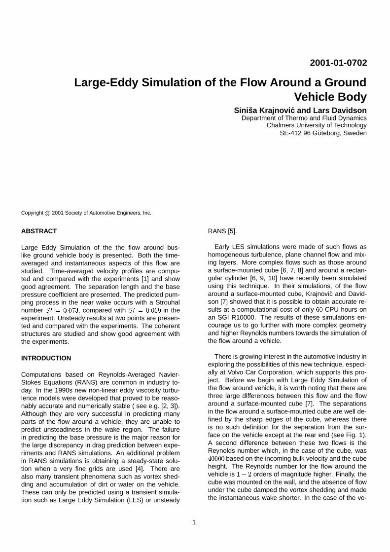
Figure 1: Geometry of the vehicle body and computational domain.

GEOMETRY AND NUMERICAL DETAILS

The geometry of the computational domain is given inFig.1. For the simulation, a domain with an upstreamlength of � � � � � � and a downstream length of� I � � � � � was used, while the span-wise width wasset at

� � �� ��� � . Similar values for upstream anddownstream lengths were found sufficient by Sohankaret al. [17] in Large Eddy Simulation of the flow arounda square cylinder. The values of other geometry quan-tities are � � �� � � m,

� � �� � �.� m,� � �� � �.� m,

� � �� ����.� m,� � �� �� � m, � � �� �� �� m, � � �� �� m

andZ � �� � m. The ground clearance of � � � � �� � � is

similar to the clearance ratio of buses. Reynolds num-ber

� � �!� �.� was � � ������� based on the incomingmean velocity,

, and the vehicle height,

�. A mesh

of ��� � million nodes was used. The time step was set to0.0002 seconds, which gave a maximum CFL numberof approximately

� � � . The CFL number was smaller thanone in � ��" of the cells. The averaging time in the simu-lation was � � � � � � � (30000 time steps). The com-putational cost using 24 SGI R10000 CPUs was � �����hours (elapsed time).

BOUNDARY CONDITIONS

Inlet boundary conditions are often obtained by doing aLarge Eddy Simulation of a channel flow. The instanta-neous velocity profile from this simulation is then usedas the inlet boundary condition. In the experimentsof Duell and George [1], the inlet mean velocity wasuniform within ��" and the average turbulent intensitywas �� �#" . A uniform velocity profile constant in timewas thus used as the inlet boundary condition in thiswork. Convective boundary conditions were applied at

the outlet. The convective boundary conditions are ofthe form $#%&�'$)( D +* $#%&�'$-,/. � � , with

�*being equal to inlet

velocity

. To simulate the moving ground, the velo-city of the lower wall was set equal to

0. The lateral

surfaces were treated as slip surfaces. The wall func-tions based on the ’instantaneous logarithmic law’ areused at all walls.

INSTANTANEOUS WALL FUNCTIONS In this work,we have not resolved the coherent structures in the nearwall region owing to high Reynolds number. These co-herent structures can be represented if the resolution is�%� � � , �V� ����� � � ��� � and ������� ��� � � � [11]. Thisrequirement implies a computational mesh in the orderof � �21 nodes [18] for the flow case presented in this pa-per. Such spatial resolution would lead to a smallertime step owing to an increased CFL number, makingwall-resolved LES of this flow infeasible. Therefore anapproximate wall boundary condition was used in thiswork. The instantaneous logarithmic law of the form�� � � � � �%�

�� � D � � � (6)

is used in the logarithmic region ( ���43 ����� ��� ). Here,�� � � �� � �� and the friction velocity is defined as ��N �� J/57698:8 � G ! �<; I . Point ��� � ����� ��� is defined as the inter-section point between the near wall linear law and thelogarithmic law. The linear law ( ��� 5 ����� ��� ) is of theform �� � �6� � � (7)

The approximate boundary condition when � � 3 ����� ���is implemented in the code by adding the artificial visco-sity, � = * , resulting from the approximate wall boundary

3

condition (6) to the laminar viscosity on the wall. Thefriction velocity, ��T , is first computed from (6). The wallshear stress is then modeled asJ 57698:8 � G�� U � C ��C � W 57698 8 � � = * �� � (8)

whereJ 57698 8

is the wall shear stress. The artificial visco-sity is now determined from the definition of the frictionvelocity and Eq. 8 as� = * � �� I ��� � �� ��� � (9)

where �� � is obtained from (6). The spatial resolutionexpressed in the wall units was ��� � ��� � ��� , �V�'� �� ��� � ����� and ����� � � ��� � ����� , as recommended byPiomelli [11].

SOME EXPERIMENTAL DETAILS

This section gives some details from the experimentsof Duell and George [1] for the purpose of comparisonwith LES. The cross section of the tunnel test sectionand the ground clearance are the same as in the LESsimulation. The location of the model front side relativeto the inlet was �� � � � m. The distance from the test sec-tion exit to the back wall perpendicular to the flow was��� � � � m. This is the back wall where Duell and Georgemounted the deflector to reduce low frequency pulsa-tions [19]. A moving ground belt and boundary layerscoop were used to simulate the floor boundary con-dition and to minimize boundary layer effects. Velocitymeasurements were done using hot wire anemometry.The velocity reported in Ref. [1] is the mean effective

cooling velocity,�������

, defined as������� � � I D � I� �<; I

where

and�

are the mean velocity components inthe � and � directions (see Fig. 1). For comparisonwith the experiments,

�������was computed in LES as������ � ��� ��� ( I D � ��� ( I � � ; I . Here,

� ��� ( and� ��� ( are time-

averaged resolved velocity components in the � and �directions obtained from LES.

RESULTS

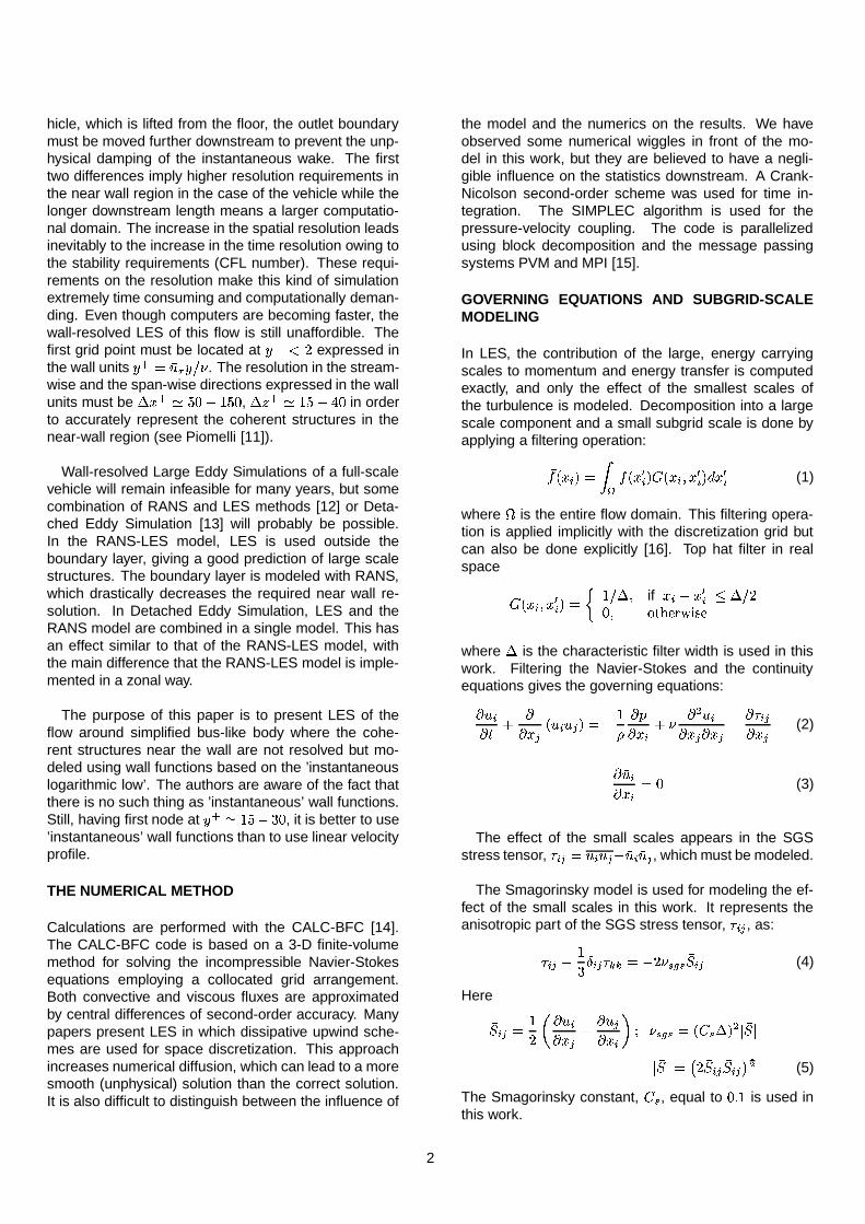
STATISTICS OF THE MEAN FLOW AND GLOBALQUANTITIES Time-averaged velocities are compu-ted and compared with the experiments. The resultsare presented in Fig. 2. As can be seen, the agree-ment with LES results is good in the recirculation region( �T� � � �� ��� , �� � � � � �2� ), while the velocity profile isunder-predicted behind the recirculation ( �� � � ��� ��� ).The location of the free stagnation point was found to bebelow the center of the base of the model at � � ��� � � ,� � ���� � � (see Fig. 3). In the experiments of Duelland George [1], the free stagnation point was assumedto be at � � � . They plotted

� ����� � along the � -axis

0 0.2 0.4 0.6 0.8 1

−0.5

0

0.5

1

PSfrag replacements

���� � � � ���

0 0.2 0.4 0.6 0.8 1

−0.5

0

0.5

1

PSfrag replacements

���� � � � �2�

0 0.2 0.4 0.6 0.8 1

−0.5

0

0.5

1

PSfrag replacements

���� � ��� ���

� ����� � Figure 2: Time-averaged velocity profiles at threedownstream locations at � � � . LES (solid line); ex-periment (symbols).

and used the local minimum as indication of the freestagnation point. The distribution of the mean velocitycomponents,

� ��� ( � and� ����� � , at � � � obtained

in our LES are plotted in Fig 4. The recirculation lengthwas found to be ��� � ��� ��� � using the local minimumof������� � + and ����� ��� ���#� using the intersection of� ��� ( � � with the � -axis. This is larger than ����� ��� � � ,

measured in the experiment of Duell and George [1].

Time-averaged velocity vectors in plane � � � areshown in Fig. 3. It can be seen that the lower entrap-ped vortex (center at ��� �� � , � � ���� � � � ) is muchsmaller than the upper vortex (center at � � � � ��� � ,� � �� � �#� ). This owing to small ground clearance,which minimizes the amount of fluid that can be entrai-ned by the lower trapped vortex [1]. Time-averaged ve-locity vectors projected onto plane � � � are shown in

4

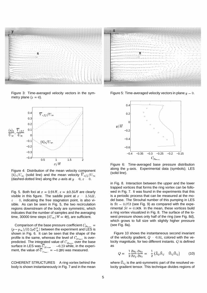
Figure 3: Time-averaged velocity vectors in the sym-metry plane ( � � � ).

0.5 1 1.5 2−0.4

−0.3

−0.2

−0.1

0

0.1

0.2

0.3

0.4

PSfrag replacements

�T� �

� ��� (+ * � ������� ��� ( �

� � � � �

Figure 4: Distribution of the mean velocity component� ��� ( � + (solid line) and the mean velocity��� � � � �

(dashed-dotted line) along the � -axis at ��� � , � � � .Fig. 5. Both foci at � � �� �� � , � � � �� � � � are clearlyvisible in this figure. The saddle point at � � ��� � �#� ,� � � , indicating the free stagnation point, is also vi-sible. As can be seen in Fig. 5, the two recirculationregions downstream of the body are symmetric, whichindicates that the number of samples and the averagingtime, 30000 time steps ( � � � � � � � ), are sufficient.

Comparison of the base pressure coefficientZ�������� �� H � H ! � � � � � G I ! between the experiment and LES is

shown in Fig. 6. It can be seen that the shape of theprofile is the same, whereas the level of

Z���� ���is over-

predicted. The integrated value ofZ���� ���

over the basesurface in LES was

Z���� ��� � ���� � � while, in the experi-ment, the value of

Z�� � ��� � ���� � ��� was measured.

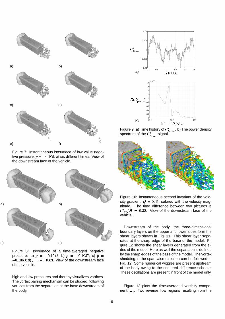
COHERENT STRUCTURES A ring vortex behind thebody is shown instantaneously in Fig. 7 and in the mean

Figure 5: Time-averaged velocity vectors in plane � � � .

−0.4 −0.35 −0.3 −0.25 −0.2 −0.15

−0.6

−0.4

−0.2

0

0.2

0.4

PSfrag replacements Z���������

��� �

Figure 6: Time-averaged base pressure distributionalong the � -axis. Experimental data (symbols); LES(solid line).

in Fig. 8. Interaction between the upper and the lowertrapped vortices that forms the ring vortex can be follo-wed in Fig. 7. It was found in the experiments that thisis a periodic process that can be measured at the mo-del base. The Strouhal number of this pumping in LESis ��� � � � � � (see Fig. 9) as compared with the expe-rimental ��� � �� ����� . In the mean, these vortices builda ring vortex visualized in Fig. 8. The surface of the lo-west pressure shows only half of the ring (see Fig. 8d),which grows to full size with slightly higher pressure(see Fig. 8a).

Figure 10 shows the instantaneous second invariantof the velocity gradient, � � �� �� , colored with the ve-locity magnitude, for two different instants. � is definedas

� � � ��

C �� �C � F C �� FC � � � � �� \ �� � F �� � F�� �/ � F �/ � F�^ (10)

where �/ � F is the anti-symmetric part of the resolved ve-locity gradient tensor. This technique divides regions of

5

a) b)

c) d)

e) f)

Figure 7: Instantaneous isosurface of low value nega-tive pressure, H � ��� � � ��� , at six different times. View ofthe downstream face of the vehicle.

a) b)

c) d)

Figure 8: Isosurface of a time-averaged negativepressure: a) H � ��� � � � � � ; b) H � ��� � � � �� ; c) H ����� � ����� ; d) H � ���� � ����� . View of the downstream faceof the vehicle.

high and low pressures and thereby visualizes vortices.The vortex pairing mechanism can be studied, followingvortices from the separation at the base downstream ofthe body.

a)0 0.5 1 1.5 2 2.5

−0.01

−0.005

0

0.005

0.01

PSfrag replacements

Z &��������� � � �������

b) 10−2

10−1

100

0

0.2

0.4

0.6

0.8

1

1.2

1.4

1.6

1.8x 10

−6

PSfrag replacements

� �"Z &�������� !��� � � � �

Figure 9: a) Time history ofZ &��� ��� . b) The power density

spectrum of theZ &������� signal.

Figure 10: Instantaneous second invariant of the velo-city gradient, � � �� �� , colored with the velocity mag-nitude. The time difference between two pictures is� + � � � � � ��� . View of the downstream face of thevehicle.

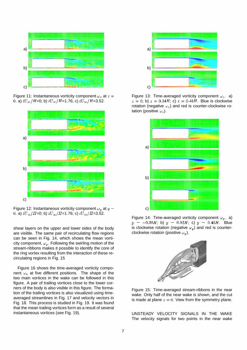
Downstream of the body, the three-dimensionalboundary layers on the upper and lower sides form theshear layers shown in Fig. 11. This shear layer sepa-rates at the sharp edge of the base of the model. Fi-gure 12 shows the shear layers generated from the si-des of the model. Here as well the separation is definedby the sharp edges of the base of the model. The vortexshedding in the span-wise direction can be followed inFig. 12. Some numerical wiggles are present upstreamof the body owing to the centered difference scheme.These oscillations are present in front of the model only.

Figure 13 plots the time-averaged vorticity compo-nent, ��� . Two reverse flow regions resulting from the

6

a)

b)

c)

Figure 11: Instantaneous vorticity component � � at � �� . a) � � � � =0; b) � � � � =1.76; c) � � � � =3.52.

a)

b)

c)

Figure 12: Instantaneous vorticity component ��� at ���� . a) � � � =0; b) � � � =1.76; c) � � � =3.52.

shear layers on the upper and lower sides of the bodyare visible. The same pair of recirculating flow regionscan be seen in Fig. 14, which shows the mean vorti-city component, ��� . Following the swirling motion of thestream-ribbons makes it possible to identify the core ofthe ring vortex resulting from the interaction of these re-circulating regions in Fig. 15

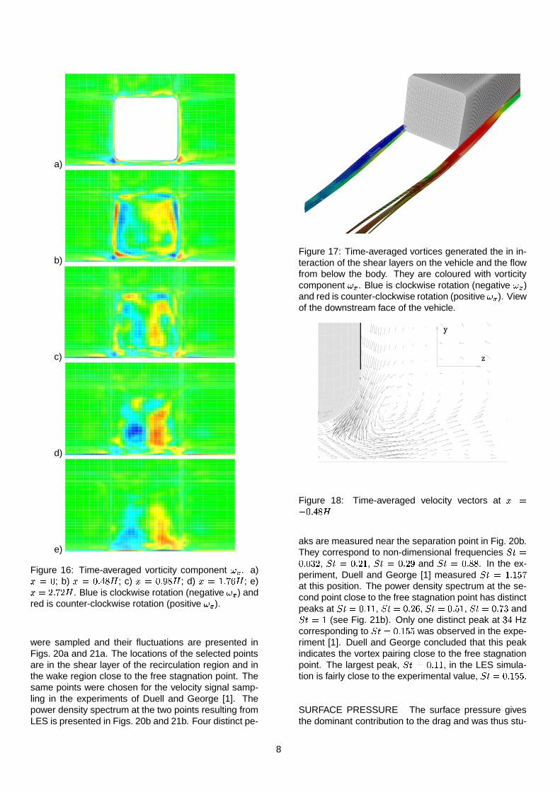
Figure 16 shows the time-averaged vorticity compo-nent � , at five different positions. The shape of thetwo main vortices in the wake can be followed in thisfigure. A pair of trailing vortices close to the lower cor-ners of the body is also visible in this figure. The forma-tion of the trailing vortices is also visualized using time-averaged streamlines in Fig. 17 and velocity vectors inFig. 18. This process is studied in Fig. 19. It was foundthat the mean trailing vortices form as a result of severalinstantaneous vortices (see Fig. 19).

a)

b)

c)

Figure 13: Time-averaged vorticity component � � . a)� � � ; b) � � �� � �#� ; c) � � � � � � � . Blue is clockwiserotation (negative � � ) and red is counter-clockwise ro-tation (positive � � ).

a)

b)

c)

Figure 14: Time-averaged vorticity component � � . a)� � ���� � � � ; b) � � �� ��� � ; c) � � �� � � � . Blueis clockwise rotation (negative ��� ) and red is counter-clockwise rotation (positive ��� ).

Figure 15: Time-averaged stream-ribbons in the nearwake. Only half of the near wake is shown, and the cutis made at plane � � � . View from the symmetry plane.

UNSTEADY VELOCITY SIGNALS IN THE WAKEThe velocity signals for two points in the near wake

7

a)

b)

c)

d)

e)

Figure 16: Time-averaged vorticity component � , . a)� � � ; b) � � � � � � � ; c) � � �� � � � ; d) � � ��� � � ; e)� � �� �� � . Blue is clockwise rotation (negative � , ) andred is counter-clockwise rotation (positive � , ).

were sampled and their fluctuations are presented inFigs. 20a and 21a. The locations of the selected pointsare in the shear layer of the recirculation region and inthe wake region close to the free stagnation point. Thesame points were chosen for the velocity signal samp-ling in the experiments of Duell and George [1]. Thepower density spectrum at the two points resulting fromLES is presented in Figs. 20b and 21b. Four distinct pe-

PSfrag replacements

Figure 17: Time-averaged vortices generated the in in-teraction of the shear layers on the vehicle and the flowfrom below the body. They are coloured with vorticitycomponent � , . Blue is clockwise rotation (negative � , )and red is counter-clockwise rotation (positive � , ). Viewof the downstream face of the vehicle.

Figure 18: Time-averaged velocity vectors at � ����� � � �

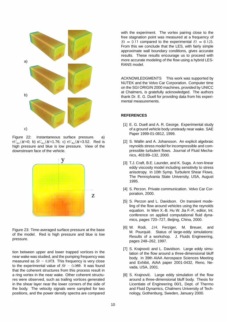
aks are measured near the separation point in Fig. 20b.They correspond to non-dimensional frequencies ��� ��� ����� , ��� � �� � � , ��� � �� � � and � � � �� � � . In the ex-periment, Duell and George [1] measured ����� ��� ����at this position. The power density spectrum at the se-cond point close to the free stagnation point has distinctpeaks at � � � �� ��� , ��� � � � ��� , ��� � � � �� , ��� � �� � and��� � � (see Fig. 21b). Only one distinct peak at � � Hzcorresponding to ��� � � � ���.� was observed in the expe-riment [1]. Duell and George concluded that this peakindicates the vortex pairing close to the free stagnationpoint. The largest peak, � � � �� ��� , in the LES simula-tion is fairly close to the experimental value, ��� � �� ��� � .SURFACE PRESSURE The surface pressure givesthe dominant contribution to the drag and was thus stu-

8

PSfrag replacements

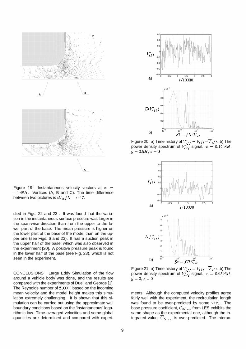
Figure 19: Instantaneous velocity vectors at � ����� � � � . Vortices (A, B and C). The time differencebetween two pictures is � � � � �� � .

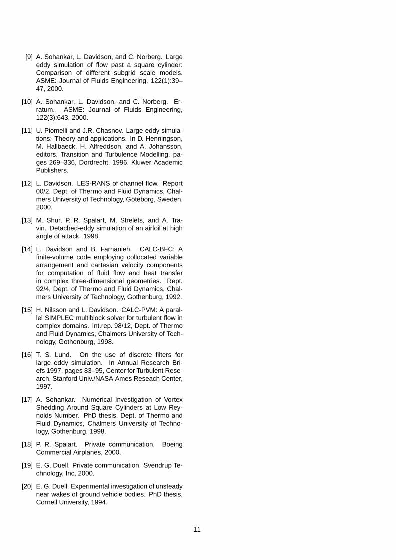
died in Figs. 22 and 23 . It was found that the varia-tion in the instantaneous surface pressure was larger inthe span-wise direction than from the upper to the lo-wer part of the base. The mean pressure is higher onthe lower part of the base of the model than on the up-per one (see Figs. 6 and 23). It has a suction peak inthe upper half of the base, which was also observed inthe experiment [20]. A positive pressure peak is foundin the lower half of the base (see Fig. 23), which is notseen in the experiment.

CONCLUSIONS Large Eddy Simulation of the flowaround a vehicle body was done, and the results arecompared with the experiments of Duell and George [1].The Reynolds number of �� ������� based on the incomingmean velocity and the model height makes this simu-lation extremely challenging. It is shown that this si-mulation can be carried out using the approximate wallboundary conditions based on the ’instantaneous’ loga-rithmic low. Time-averaged velocities and some globalquantities are determined and compared with experi-

a)0 0.5 1 1.5 2 2.5 3

−0.4

−0.3

−0.2

−0.1

0

0.1

0.2

0.3

PSfrag replacements

� &������ � � �������

b) 10−2

10−1

100

101

0

0.2

0.4

0.6

0.8

1x 10

−3

PSfrag replacements

� � � &� � � !��� � � � � +

Figure 20: a) Time history of� &� � � � � ����� � ������� . b) The

power density spectrum of� &����� signal. � � � � � � ��� � ,��� �� � � , � � �

a)0 0.5 1 1.5 2 2.5 3

−0.2

−0.1

0

0.1

0.2

0.3

0.4

PSfrag replacements

� &������ � � �������

b) 10−2

10−1

100

101

0

1

2

3

4

5

6

7

x 10−4

PSfrag replacements

� � � &����� !� � � � � �

Figure 21: a) Time history of� &� � � � � ����� � ������� . b) The

power density spectrum of� &����� signal. � � � � ����� � � ,��� � , � � �

ments. Although the computed velocity profiles agreefairly well with the experiment, the recirculation lengthwas found to be over-predicted by some � � " . Thebase pressure coefficient,

Z ��������, from LES exhibits the

same shape as the experimental one, although the in-tegrated value,

Z � ������, is over-predicted. The interac-

9

a)

b)

c)

Figure 22: Instantaneous surface pressure. a)� + � � =0; b) � � � � =1.76; c) � � � � =3.52. Red ishigh pressure and blue is low pressure. View of thedownstream face of the vehicle.

Figure 23: Time-averaged surface pressure at the baseof the model. Red is high pressure and blue is lowpressure.

tion between upper and lower trapped vortices in thenear wake was studied, and the pumping frequency wasmeasured as ��� � � � � � . This frequency is very closeto the experimental value of ��� � � � ����� . It was foundthat the coherent structures from this process result ina ring vortex in the near wake. Other coherent structu-res were observed, such as trailing vortices generatedin the shear layer near the lower corners of the side ofthe body. The velocity signals were sampled for twopositions, and the power density spectra are compared

with the experiment. The vortex pairing close to thefree stagnation point was measured at a frequency of��� � �� ��� compared to the experimental ��� � �� ��� � .From this we conclude that the LES, with fairly simpleapproximate wall boundary conditions, gives accurateresults. These results encourage us to proceed withmore accurate modeling of the flow using a hybrid LES-RANS model.

ACKNOWLEDGMENTS This work was supported byNUTEK and the Volvo Car Corporation. Computer timeon the SGI ORIGIN 2000 machines, provided by UNICCat Chalmers, is gratefully acknowledged. The authorsthank Dr. E. G. Duell for providing data from his experi-mental measurements.

REFERENCES

[1] E. G. Duell and A. R. George. Experimental studyof a ground vehicle body unsteady near wake. SAEPaper 1999-01-0812, 1999.

[2] S. Wallin and A. Johansson. An explicit algebraicreynolds stress model for incompressible and com-pressible turbulent flows. Journal of Fluid Mecha-nics, 403:89–132, 2000.

[3] T.J. Craft, B.E. Launder, and K. Suga. A non-lineareddy viscosity model including sensitivity to stressanisotropy. In 10th Symp. Turbulent Shear Flows,The Pennsylvania State University, USA, August1995.

[4] S. Perzon. Private communication. Volvo Car Cor-poration, 2000.

[5] S. Perzon and L. Davidson. On transient mode-ling of the flow around vehicles using the reynoldsequation. In Wen X.-B. Hu W. Jia F.-P., editor, Int.conference on applied computational fluid dyna-mics, pages 720–727, Beijing, China, 2000.

[6] W. Rodi, J.H. Ferziger, M. Breuer, andM. Pourquie. Status of large-eddy simulations:Results of a workshop. J. Fluids Engineering,pages 248–262, 1997.

[7] S. Krajnovic and L. Davidson. Large eddy simu-lation of the flow around a three-dimensional bluffbody. In 39th AIAA Aerospace Sciences Meetingand Exhibit, AIAA paper 2001-0432, Reno, Ne-vada, USA, 2001.

[8] S. Krajnovic. Large eddy simulation of the flowaround a three-dimensional bluff body. Thesis forLicentiate of Engineering 00/1, Dept. of Thermoand Fluid Dynamics, Chalmers University of Tech-nology, Gothenburg, Sweden, January 2000.

10

[9] A. Sohankar, L. Davidson, and C. Norberg. Largeeddy simulation of flow past a square cylinder:Comparison of different subgrid scale models.ASME: Journal of Fluids Engineering, 122(1):39–47, 2000.

[10] A. Sohankar, L. Davidson, and C. Norberg. Er-ratum. ASME: Journal of Fluids Engineering,122(3):643, 2000.

[11] U. Piomelli and J.R. Chasnov. Large-eddy simula-tions: Theory and applications. In D. Henningson,M. Hallbaeck, H. Alfreddson, and A. Johansson,editors, Transition and Turbulence Modelling, pa-ges 269–336, Dordrecht, 1996. Kluwer AcademicPublishers.

[12] L. Davidson. LES-RANS of channel flow. Report00/2, Dept. of Thermo and Fluid Dynamics, Chal-mers University of Technology, Goteborg, Sweden,2000.

[13] M. Shur, P. R. Spalart, M. Strelets, and A. Tra-vin. Detached-eddy simulation of an airfoil at highangle of attack. 1998.

[14] L. Davidson and B. Farhanieh. CALC-BFC: Afinite-volume code employing collocated variablearrangement and cartesian velocity componentsfor computation of fluid flow and heat transferin complex three-dimensional geometries. Rept.92/4, Dept. of Thermo and Fluid Dynamics, Chal-mers University of Technology, Gothenburg, 1992.

[15] H. Nilsson and L. Davidson. CALC-PVM: A paral-lel SIMPLEC multiblock solver for turbulent flow incomplex domains. Int.rep. 98/12, Dept. of Thermoand Fluid Dynamics, Chalmers University of Tech-nology, Gothenburg, 1998.

[16] T. S. Lund. On the use of discrete filters forlarge eddy simulation. In Annual Research Bri-efs 1997, pages 83–95, Center for Turbulent Rese-arch, Stanford Univ./NASA Ames Reseach Center,1997.

[17] A. Sohankar. Numerical Investigation of VortexShedding Around Square Cylinders at Low Rey-nolds Number. PhD thesis, Dept. of Thermo andFluid Dynamics, Chalmers University of Techno-logy, Gothenburg, 1998.

[18] P. R. Spalart. Private communication. BoeingCommercial Airplanes, 2000.

[19] E. G. Duell. Private communication. Svendrup Te-chnology, Inc, 2000.

[20] E. G. Duell. Experimental investigation of unsteadynear wakes of ground vehicle bodies. PhD thesis,Cornell University, 1994.

11