large scale inference under sparse and weak alternatives

Large scale inference undersparse and weak alternatives:non-asymptotic phasediagram for CsCsHMstatistics

OSKAR STATTIN

Master in Applied and Computational MathematicsDate: June 27, 2017Supervisor: Tatjana PavlenkoExaminer: Tatjana PavlenkoSwedish title: Storskalig inferens för glesa och svaga alternativ:icke-asymptotiska fasdiagram för CsCsHM-testvariablerSchool of Engineering Sciences

iii

Abstract

Modern mätteknologi tillåter att generera och lagra gigantiska mängderdata, varav en stor andel är redundanta och varav bara ett fåtal är an-vändbara för ett givet problem. Områden där detta är vanligt är tillexempel inom genomik, proteomik och astronomi, där stora multi-pla test ofta behöver utföras, med förväntan om endast några fåsig-nifikanta effekter. Ett antal nya testprocedurer har utvecklats för atttesta dessa så-kallade svaga och glesa effekter i storskalig statistisk in-ferens. Den mest populära av dessa är troligen Higher Criticism, HC(se Donoho och Jin (2004)). En ny klass av goodness-of-fit-testvariabeldöpt CsCsHM har nyligen blivit härledd (se Stepanova och Pavlenko(2017)) för samma typ av multipla testscenarion och har bevisat bättreasymptotiska egenskaper än den traditionella HC-metoden.

Den här rapporten utforskar det empiriska beteendet för båda test-metodikerna i närheten av detektionsgränsen, vilken är tröskeln fördetektion av glesa och svaga effekter. Den här teoretiska, skarpa gränsendelar fasrymden, vilken är uppspänd av gleshets- och svaghetsparame-trarna, i två delområden: det detektionsbara och det icke-detektionsbaraområdet. Testsvariablernas metodik tillämpas även för variabelselek-tion för storskalig binär klassificering. Dessa tillämpas, förutom simu-leringar, på riktig data. Resultaten pekar på att testvariablerna är jäm-förbara i prestation.

iv

Abstract

High-throughput measurement technology allows to generate and storehuge amounts of features, of which very few can be useful for anyone single problem at hand. Examples include genomics, proteomicsand astronomy, where massive multiple testing often needs to be per-formed, expecting a few significant effects and essentially a null back-ground. A number of new test procedures have been developed fordetecting these, so-called sparse and weak effects, in large scale sta-tistical inference. The most widely used is Higher Criticism, HC (seee.g. Donoho and Jin (2004)). A new class of goodness-of-fit test statis-tics, called CsCsHM, has recently been derived (see Stepanova andPavlenko (2017)) for the same type of multiple testing, it is shown toachieve better asymptotic properties than the traditional HC approach.

This report empirically investigates the behavior of both test proce-dures in the neighborhood of the detection boundary, i.e. the thresholdfor the detectability of sparse and weak effects. This theoretical bound-ary sharply separates the phase space, spanned by the sparsity andweakness parameters, into two subregions: the region of detectabil-ity and the region of undetectability. The statistics are also appliedand compared for both methodologies for features selection in highdimensional binary classification problems. Besides the study of themethods and simulations, applications of both methods on realisticdata are carried out. It is found that the statistics are comparable inperformance accuracy.

Contents

1 Introduction 11.1 Problem statement . . . . . . . . . . . . . . . . . . . . . . 21.2 Outline . . . . . . . . . . . . . . . . . . . . . . . . . . . . . 2

2 Background 32.1 Higher criticism in signal detection . . . . . . . . . . . . . 3

2.1.1 A general framework for signal detection . . . . . 32.1.2 Higher criticism . . . . . . . . . . . . . . . . . . . 72.1.3 CsCsHM as an alternative testing procedure . . . 11

2.2 Variable selection with higher criticism . . . . . . . . . . 142.2.1 Phase diagram for classification . . . . . . . . . . 152.2.2 Higher criticism thresholding . . . . . . . . . . . . 172.2.3 Variable selection using CsCsHM . . . . . . . . . 18

2.3 Extensions of higher criticism . . . . . . . . . . . . . . . . 19

3 Numerical study 223.1 Signal detection . . . . . . . . . . . . . . . . . . . . . . . . 22

3.1.1 Methods . . . . . . . . . . . . . . . . . . . . . . . . 223.1.2 Results . . . . . . . . . . . . . . . . . . . . . . . . . 24

3.2 Classification . . . . . . . . . . . . . . . . . . . . . . . . . . 273.2.1 Methods . . . . . . . . . . . . . . . . . . . . . . . . 283.2.2 Results . . . . . . . . . . . . . . . . . . . . . . . . . 30

4 Discussion 34

v

Chapter 1

Introduction

As storage grows cheaper and data exponentially bigger, fast com-putational methods are needed to keep up. When acquiring data itis, with the availability of large storage and modern high throughputmeasurement technology, easy to measure a large number of variableswithout necessarily expecting a signal in any but a few of them. Thisphenomenon is sometimes called data glut and gives rise to a new kindof problem of massive multiple testing for significances against a nullbackground. For some data types, such as microarrays of DNA orproteins, which are naturally huge in dimension, sometimes having asmany as ∼ 106 entries, this is an essential part of the analysis.

When testing multiple hypotheses, i.e that we have a non-zero sig-nal in any of the variables, we need to take into consideration the pos-sibility that one or several of the variables are significant as by chance,and not by merit. John Tukey suggested a testing method on a metalevel or a higher level, which he called Higher Criticism (HC) to accountfor this phenomenon. Its purpose was to test the overall body of testsfor a fixed significance. This idea was the basis for the HC type statisticproposed by Donoho and Jin in 2004 [1].

HC has since evolved and today there exists many different adap-tations for various applications, two of these applications are signaldetection [1] [2] and feature selection for classification [3] [4] [5]. Seethe symposium by Donoho and Jin for a comprehensive overview [6].The HC framework has proved especially useful for very large data,because of its cheap computational properties, light overhead and sta-tistical interpretability. It is a non-parametric method so it requireslittle to no tuning.

1

2 CHAPTER 1. INTRODUCTION

However there is a known problem with the asymptotics of HC,where the test statistic goes to infinity in probability as the samplesize goes to infinity under H0. To amend this problem Stepanova andPavlenko used results from studies of empirical weighted processesto suggest a new statistic which has better asymptotical properties,see [2]. This new statistic is called after the mathematicians Csörgos,Csörgos, Horváth and Mason, abbreviated CsCsHM.

1.1 Problem statement

In this report we aim to answer how CsCsHM behaves for finite sam-ple size in comparison to HC. This is done in a way inspired by Blomberg[7], with the the primary tool being heat maps of an empirical errormeasure over the phase space spanned by the sparsity and weaknessparameters.

Two scenarios are considered: signal detection and variable selec-tion for binary classification. The second is in some way an extensionof the former, for which CsCsHM is adapted. Besides simulations, ap-plications of both HC and CsCsHM on realistic data are performed forvariable selection for classification.

1.2 Outline

This report consists of three main parts, the chapter 2: Backgroundwhere the theoretical justifications for the work is presented alongsidesome orienting results on related topics. After this starting point, inthe chapter 3: Numerical study the simulations and experiments per-formed are presented with methods and results. Finally the results arediscussed and some conclusions are drawn in chapter 4: Discussion.

Chapter 2

Background

In this section an introduction to the theoretical results and definitionsunderlying the experiments are presented. For a more thorough back-ground, see the cited sources, especially the works by Donoho and Jin.

2.1 Higher criticism in signal detection

Signal detection is the task of finding whether there exists a signalamong the noise in a dataset. This can be formalized as a hypothesistesting scenario where the null hypothesis H0 is that there is no signal,so the distribution consists of only noise. The alternative hypothesisH1 is that a small fraction of the signals come from another separatedistribution.

2.1.1 A general framework for signal detection

In the introduction it was mentioned that HC is used in scenarioswhere we have weak and sparse signals. This is formalized as therare and weak (RW) framework which is based on two hypotheses.

The first hypothesis is of effect sparsity. It states that only a few ofthe observed signals are expected to differ from a global null hypothe-sis that everything is noise, meaning that the true signals are rare. Thesecond hypothesis is of effect weakness, and states that the signals arehard to detect since they are weak.

Together these two hypotheses give us the challenging situation ofhaving only a few informative signals among many non-informative,and these signals are hard to distinguish from each other.

3

4 CHAPTER 2. BACKGROUND

This framework can be incorporated into a mixture model of twodistributions F and G, where the former is the non-informative, andthe latter is the informative distribution. This can be written as

X ∼ (1− ε)F + εG, (2.1)

meaning that a vector X = (X1, . . . , Xn) has each component indepen-dently and identically distributed drawn from one of the two distribu-tions. The number of components of the feature vector, n, is large. Theepsilon denotes the fraction of the components which are informativeε ∈ (0, 1), and is according to the sparsity hypothesis small.

For our purposes we will look at a mixture of the same type of dis-tribution, where G has a slightly shifted mean but the same variance.Using the notation from 2.1 and integrating the mixture model into thehypothesis testing of signal detection, it can be written as

H0 : Xi ∼ F, (2.2)

H(n)1 : Xi ∼ (1− ε)F + εG. (2.3)

By specifying the distributions of F and G as normal distributions, wearrive at the n individual tests,

H0,i : Xi ∼ N (0, 1), (2.4)H1,i : Xi ∼ N (µ0, 1), µ0 > 0. (2.5)

Here the null hypothesis H0 is that there are no signals among all thesignals, so the intersection of H0,1 ∩H0,2 ∩ · · · ∩H0,n. The alternative isthat there are signals, so that some H1,i is true. We write this as

H0 : Xi ∼ N (0, 1), (2.6)

H(n)1 : Xi ∼ (1− ε)N (0, 1) + εN (µ0, 1), (2.7)

where µ0 is a small shift in mean and ε is as above. Further we as-sume that the signals are independently and identically distributed,and share a common amplitude and variance. In this framework,which we call RW (ε, µ0) we can test the null hypothesis, that the ob-servations only consist of noise.

CHAPTER 2. BACKGROUND 5

The phase space of β and r

A natural way to investigate the results of signal detection is to lookat the borderland where the signals are so weak or sparse that it be-comes nearly impossible to separate signal from noise. However theparametrization of RW (ε, µ0) makes for awkward values in the areaclose to where detection is impossible. Introducing the sparsity pa-rameter β and strength parameter r in the following way allows for amore handy phase space on the domain (0, 1)× (0, 1).

The sparsity parameter β is defined by

ε = n−β. (2.8)

This parameter leads to a natural partition of a dense region where0 < β ≤ 0.5 and a sparse region where 0.5 < β < 1. In these tworegions the strength parameter is chosen differently, since differentgrowth rates are interesting for the two paradigms. The strength pa-rameter r is defined by

µ0 =

n−r 0 < β ≤ 0.5, 0 < r < 0.5,√

2r log(n) 0.5 < β < 1, 0 < r < 1.(2.9)

This gives us a region of undefined quadratical space in the denseregion 0 < β < 0.5 where 0.5 < r < 1, where the signals are too weakwith this parametrization to be interesting. See Figure 2.1 below for avisualization of the different areas.


Figure 2.1: The phase diagram for signal detection with the detectionboundary for the dense and sparse areas. Blue denotes the area ofdetectability, and red the area of non-detectability.

The detection boundary

In the phase space spanned by these two parameters a theoretical limitcalled the detection boundary, deduced by Ingester [8], separates thespace into two regions: a region of undetectability and a region ofdetectability. Detection is impossible below and possible above thisthreshold, why the areas are sometimes called the regions of failureand success respectively.

For the normal mixture case the detection boundary has been provento be


ρ∗(β) =

1− β 0 < β ≤ 0.5,

β − 0.5 0.5 < β < 0.75,

1− (1−√β)2 0.75 < β < 1.

(2.10)

Detection is thus possible wherever this boundary is exceeded by r, i.er > ρ∗(β), see [1].

2.1.2 Higher criticism

Donoho and Jin suggested in 2004 a procedure called "Higher Criti-cism", or HC, for testing in the RW -scenario of normal distributions[1]. Inspired by and named after John Tukey’s ideas of a higher-ordertesting, the motivation for the proposed statistic was to compare theexpected number of significant tests to the actual number. Instead oflooking at individual tests’ significance, the significance of the overallbody of tests is used, making it a second-order or higher type of testing.

In Tukey’s proposed method, one decides upon a significance level,say α = 0.05, and the statistic is then formed as

HCn,0.05 =√n

(Fraction significant at 5%− 0.05)√0.05× 0.95

. (2.11)

Donoho and Jin generalized this to include a wider range of signif-icances, over all levels with a selected upper bound α0, letting theirHC-statistic become

HCn,α =√n

(Fraction significant at α− α)√α× (1− α)

. (2.12)

If the body of tests is significant, then this statistic is expected to belarge for some α, and if it is not, then it is expected to be small for allα:s. Thus the maximum value over all ranges of α was chosen as thetest statistic for the significance of the body of tests:

HC∗n = max0<α<α0

HCn,α

. (2.13)

This test statistic is then compared to a critical value, and if this valueis exceeded the null hypothesis is rejected and a signal is considereddetected.


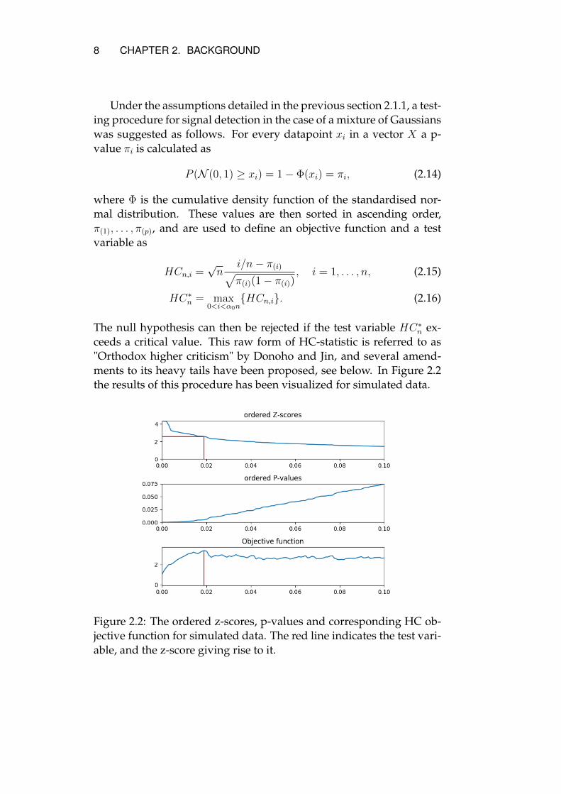
Under the assumptions detailed in the previous section 2.1.1, a test-ing procedure for signal detection in the case of a mixture of Gaussianswas suggested as follows. For every datapoint xi in a vector X a p-value πi is calculated as

P (N (0, 1) ≥ xi) = 1− Φ(xi) = πi, (2.14)

where Φ is the cumulative density function of the standardised nor-mal distribution. These values are then sorted in ascending order,π(1), . . . , π(p), and are used to define an objective function and a testvariable as

HCn,i =√n

i/n− π(i)√π(i)(1− π(i))

, i = 1, . . . , n, (2.15)

HC∗n = max0<i<α0n

HCn,i. (2.16)

The null hypothesis can then be rejected if the test variable HC∗n ex-ceeds a critical value. This raw form of HC-statistic is referred to as"Orthodox higher criticism" by Donoho and Jin, and several amend-ments to its heavy tails have been proposed, see below. In Figure 2.2the results of this procedure has been visualized for simulated data.

Figure 2.2: The ordered z-scores, p-values and corresponding HC ob-jective function for simulated data. The red line indicates the test vari-able, and the z-score giving rise to it.


Two attractive properties of this method is firstly that it does notrequire any information about the parameters ε or µ0 in contrast toother approaches such as likelihood-ratio tests. This is dubbed opti-mal adaptivity. Secondly, the testing is performed at a moderate cost,O(n log n).

Properties of higher criticism

To better understand the objective function we can see it as a compar-ison of the expected fraction of observed significances under the nullhypothesis to the actual fraction of observed significances. The nomi-nator thus captures the difference between this expected behaviour ofthe p-values and their actual behaviour, and is similar to the Kolmogorov-Smirnov (KS) statistic.

A KS test variable Kn over a continuous variable x ∈ R is formedas

Kn :=√n sup

x|Fn(x)− F (x)|, (2.17)

where F (x) is the theoretical cumulative density function in x, and Fnis the empirical distribution function (EDF) defined as

Fn(x) =1

n

n∑i=1

1Xi < x. (2.18)

Closely related is the goodness-of-fit measure suggested by Andersonand Darling [9] which utilizes a similar structure, but squared insteadof absolute valued and with a normalizing function ψ(x),

ADn,ψ = n

∫ ∞−∞

(Fn(x)− F (x))2ψ(F (x))f(x)dx. (2.19)

Here the ψ(x) is introduced as a type of normalizing function, andf(x) is the probability density function in x. Under the null hypoth-esis we have that nFn ∼ Bin(n, F (x)), so the variance is known to beV ar(Fn(x)) = 1

nF (x)(1−F (x)). With this as normalizing function, and

using an L∞ norm we arrive at the HC statistic with α0 = 1. For detailssee [10]. HC is thus rooted in similar statistics and not an isolated idea.

Donoho and Jin suggests two different normalizations for HC of


this form,

HC2004 = max1<i<α0n

√n

i/n− π(i)√π(i)(1− π(i))

, (2.20)

HC2008 = max1<i<α0n

√ni/n− π(i)√in(1− i

n). (2.21)

For an approach from the goodness-of-fit angle, see [11] where severaldifferent normalizations are considered and analyzed.

Under the global null the expected distribution of the p-values isuniform, so we expect to see Un(u) = 1

n

∑ni=1 1Ui < u, where Ui ∼

U(0, 1) being iid random variables, as the EDF. For a sequence of iidrandom variables X1, X2, . . . Xn with a continuous cumulative distri-bution function F on R the EDF can then be approximated as Fn(i) =

i/n for the i:th p-value, according to the assumption that the p-valuesare uniformly distributed.

It has been noticed that convergence of test statistics on this formHC(u) =

√n(Un(u) − u)/

√u(1− u) depend on their behaviour close

to one and zero. Therefore a practical modification is to truncate thelower interval over which the u:s are taken, for example (1/n, α0). Thisgives rise to a new test variable

HC+ = max1/n<u<α0

HCn(u), (2.22)

where the right hand side can be on the form of any of HC2008 orHC2004. However this alleviates the problem for finite samples sizesonly, as it has been shown that

limn→∞

P (an sup0<u<α0

√n

(Un(u)− u)√u(1− u)

− bn ≤ x) = e−12e−x

, (2.23)

where an =√

2 log log n and bn = 2 log log n+1/2 log log log n−1/2 log(4π).The right hand side is the Gumbel distribution. Similar results can beshown for other truncated intervals, see [2]. This means that no matterthe chosen interval, the extreme value distribution is reached and thestatistic will tend to infinity for large enough n under H0.

This has motivated research to find other statistics either by a dif-ferent normalization, like the CsCsHM-statistic [2], or by ordered statis-tics such as the exact Berk-Jones statistic [10].


Determining the critical value and choice of test statistic

To use HC as a test on significance level α, we need a critical valueh(n, α) that satisfies

P (HC∗n > h(n, α)|H0) = α. (2.24)

As usual in hypothesis testing, the test statistic is calculated and if itexceeds this critical value, then the null is rejected in favour of thealternative hypothesis. To find this threshold, Theorems 1.1 and 1.2from Donoho and Jin [1] are used. The former theorem states thatunder the null hypothesis H0 the following holds,

HC∗n√2 log log n

p→ 1, n→∞. (2.25)

The second theorem states that for a sequence of problems indexed byn where αn → 0 so slowly that h(n, αn) =

√2 log log n(1 + o(1)), then a

HC-test that rejects the null H0 when HC∗n > h(n, αn), has full powerwhen every alternative H(n)

1 is defined so that r > ρ∗(β). This meansthat the probability of rejecting the null hypothesis goes to one underevery H(n)

1 in the region of detectability as n goes to infinity,

P (Reject H0|H(n)1 )→ 1, n→∞. (2.26)

The HC test procedure is consistent against all alternatives and has fullpower in the region of detectability, if the threshold is taken for a fixedα as

h(n, α) =√

2 log log n(1 + o(1)), (2.27)

where the o(1) is a buffer since the results are asymptotical. Numericalsimulations show that this estimation can be of varying satisfaction.However this means that HC has the property of optimal adaptivity.

The error rate of the HC procedure in the area of detectability isnot necessary zero for finite size samples. It has been shown that thereis no perfectly sharp boundary where it suddenly becomes impossibleto detect signals, but rather a blurry area of transition between successand failure, see [7].

2.1.3 CsCsHM as an alternative testing procedure

A solution to the problem of the HC-statistic converging to an extremevalue distribution was proposed by Stepanova and Pavlenko in [2]. By


using a normalization with roots in results for weighted empirical pro-cesses, the test variable converges to a brownian bridge in distributionas the sample size goes to infinity. The new statistic is named after themathematicians Csörgo, Csörgo, Horváth and Mason, or CsCsHM forshort.

The results are based on what are called Erdos-Feller-Kolmogorov-Petrovski (EFKP) upper class functions of Brownian bridges, B(u), 0 ≤u ≤ 1, of which an important one is

q(u) =√u(1− u) log log(1/(u(1− u))). (2.28)

This example comes from Khinchine’s local law of the iterated loga-rithm which states that

lim supu→0

W (u)√u log log(1/u)

a.s.=√

2, (2.29)

whereW (u) is a standard Wiener process starting at zero. Relating thisto the Brownian bridge, B(u), 0 ≤ u ≤ 1 D

= W (u)− uW (u), 0 ≤ u ≤1, we have that

lim supu→0

|B(u)|√u(1− u) log log(1/(u(1− u))

a.s.=√

2. (2.30)

Using these observations as a starting point in the testing scenario H0 :

F = F0 versus the alternative H1 : F > F0, the following test statisticis suggested

T+n (q) = sup

0<F0(t)<1

√nFn(t)− F0(t)

q(F0(t)). (2.31)

As detailed in Proposition 3.1 in [2], it is shown that this statis-tic with slightly different demands on F0(t) will converge in distri-bution to a normalized Brownian bridge. If q is an EFKP upper-class function of a Brownian bridge, then under H0 for any numbers0 ≤ a < b ≤ 1 as n→∞,

supa<F0(t)<b

√n

(Fn(t)− F0(t))

q(F0(t))

D→ supa<u<b

B(u)

q(u). (2.32)

This gives us a theoretical justification of truncating the interval overwhich the statistic is formed, (0, α0), and the interpretation of this in-terval as the body of significances which are becomes clearer.


For this setting, a test of asymptotic level α that rejects H0 when

T+n (q) ≥ t+α (q), (2.33)

where t+α (q) is chosen such that P (sup0<u<1B(u)/q(u) ≥ t+α (q)) = α.Then for every alternative H i

n in the area of detectability, i.e r > ρ(β),the test based on T+

n (q) has full power, meaning that

P (T+n (q) ≥ t+α (q)|H i

n)→ 1, n→∞. (2.34)

This means that asymptotically, the CsCsHM testing procedure willbe able to perfectly separate cases where there are signals and wherethere are not, as long as the strength of the signal exceeds the detec-tion boundary. This means CsCsHM also has the property of optimaladaptivity.

To choose the specific threshold, there are tabulations of the distri-bution of the random variable sup0<u<1B(u)/q(u).

Two applied variants of this proposed statistic, with the same test-ing procedure for signal detection as the one for HC described previ-ously, are

CsCsHM1(π(i)) =

√n(i/n− π(i))√

πi(1− π(i)) log(log( 1π(i)(1−π(i))

))1 ≤ i ≤ n,

(2.35)

CsCsHM2(π(i)) =

√n(i/n− π(i))√

πi(1− π(i)) log(log( 1π(i)(1−π(i))

)), 1 ≤ i ≤ n,

(2.36)

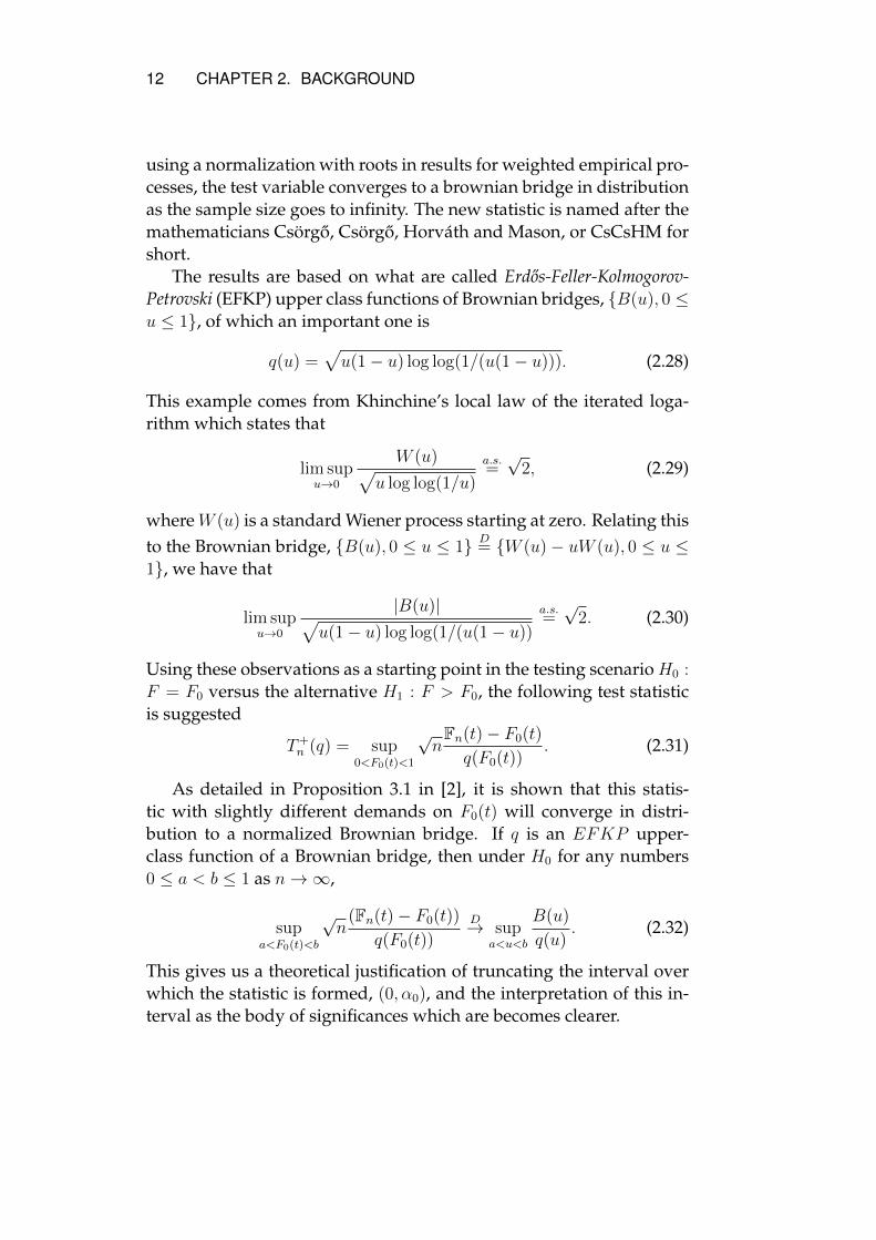
where the difference lies in the square root in the denominator. Whenfinding the maximum of these two a restriction of size of the π(i):s,similar to the one for HC, can be enforced. For a similar depiction ofthe z-scores and p-values as previously shown for HC, see Figure 2.3below.


Figure 2.3: The ordered z-scores, p-values and correspondingCsCsHM1 objective function for simulated data. The red line indicatesthe test variable, and the z-score giving rise to it.

2.2 Variable selection with higher criticism

Two natural extensions of signal detection are to be able to identifyvariables containing a signal, and to recover these signals. The focus isstill on the interesting rare and weak framework with the dimension-ality being much larger than the number of samples, p >> n. Noticethat we revert to the notation of dimension as p and samples as n.

In binary classification we have n samples from a population. Eachone of these consists of p dimensions, where each individual sampleXi

comes from one of two classes, Yi ∈ c1, c2. To represent this a matrixof size (n × p), called X = (X1, . . . , Xn)T is used, where every rowXi = (xi1, . . . , xip) represents one sample. We will assume that eachrow of X is independently and identically distributed. The correlationmatrix will be assumed to be identity.

The goal of classification is to learn a predictor from training data,that determines the classes of test data as well as possible.

According to the hypotheses of sparsity and weakness only a smallnumber of the p variables will be informative, and among these thecontrast mean (the difference in mean between the classes) will besmall. Instead of using all the variables when performing classifica-


tion, which could potentially be very computationally costly, variableselection opts to find the ones that seem to impact the choice of class ofthe samples the most. To select the variables, the HC framework canbe employed.

2.2.1 Phase diagram for classification

While the scenario is similar for the two cases of variable selection andsignal detection, the detection boundary will be slightly different forclassification. This is because the number of samples will influencethe boundary in the phase diagram spanned by (β, r). The effect isdepicted in Figure 2.4. The phase diagram will include several regionswhere success is possible, probable or outright impossible.

Figure 2.4: The effect of θ on the detection boundary for classification.

The question is whether a trained classifier can successfully clas-sify data given a set of parameters in the phase space. As mentionedthe amount of samples n comes into play, so a new parameter θ link-ing dimensionality and sample size is defined as n = pθ. We assumebalanced data between classes n1 = n2 = pθ/2.

HC thresholding achieves the optimal detection boundary for clas-


sification, which can be written for 0 < β < 1− θ as

ρ∗C(β) = (1− θ)ρ∗( β

1− θ), (2.37)

as proved by Donoho and Jin [3]. Below this boundary all classifiers’misclassification rate tends to 1/2, which is equivalent to guessing thelabels of the test data. For different growth rates of θ, see [5] for adetailed exposition.

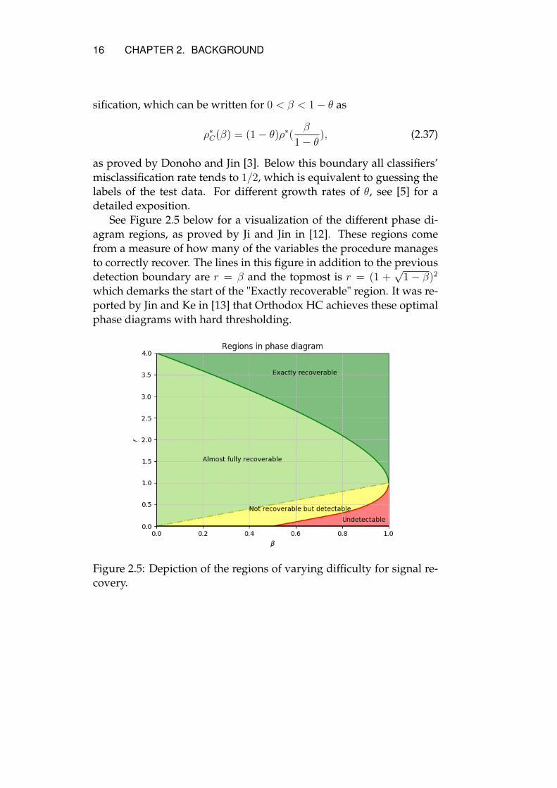
See Figure 2.5 below for a visualization of the different phase di-agram regions, as proved by Ji and Jin in [12]. These regions comefrom a measure of how many of the variables the procedure managesto correctly recover. The lines in this figure in addition to the previousdetection boundary are r = β and the topmost is r = (1 +

√1− β)2

which demarks the start of the "Exactly recoverable" region. It was re-ported by Jin and Ke in [13] that Orthodox HC achieves these optimalphase diagrams with hard thresholding.

Figure 2.5: Depiction of the regions of varying difficulty for signal re-covery.


2.2.2 Higher criticism thresholding

For HC thresholding (HCT), the labels will be defined as Y ∈ −1, 1,and the data modelled as coming from the following distribution,

Xi ∼ N (µi · Yi, In), (2.38)

where the covariance matrix In is identity, and µi is the contrast meanbetween the two classes. We will also assume that the prior probabilityfor each class is equal.

A type of feature score similar to a t-statistic is formed, defined as

Zj =1√n

n∑i=1

(Yi · xij), (2.39)

where the size of the score will be big in absolute terms if the con-trast mean is big, and small otherwise. We obtain two-sided p-valuesπi = P (|N (0, 1)| ≥ |Zi|) = 2Φ(|Zi|) for all the feature scores Zjpj=1.Similarily to before, we sort these in ascending order, π(1), . . . , π(p) , andform the HC objective function for the transformed scores:

HC(i, π(i)) =√p

i/p− π(i)√i/p(1− i/p)

, 1 ≤ i ≤ p. (2.40)

This is the statistic we previously called HC2008 in Eq. 2.21 which wasproposed by Donoho and Jin in 2008 in [4]. This objective function can,as discussed, be exchanged for another HC-type statistic with somedifferent normalization.

The maximizing index of the objective function is found,

iHC = arg max1≤i≤p

HC(i, π(i)), π(i) ∈ (εs, 0.1) (2.41)

where we have introduced a restriction on the size of the p-values.The value of the Z(j) (where we have an ordering in the same way asfor the S(i) values) corresponding to the index iHC is then taken as thethreshold value,

tHCp = |Z|(iHC). (2.42)

Once the threshold is decided, it is used in a threshold function thatchooses which variables to consider. A function of this kind is the hardthreshold function, defined as ηhardt (zi) = sgn(Zi)1|Zi|>t.


One easy way to predict the classes when the interesting variableshave been selected, is by using a discriminant rule. Then the class of agiven sample is given by the sign of L(Xi), given by

L(Xi) =

p∑j=1

wt(j)xij, (2.43)

where wt(j) = ηhardt (zj). This is a case of linear discriminant analy-sis, LDA, see Hastie, Tibshirani, Friedman [14] and references therein.There are other ways to treat the remaining selected variable but thisclassifier will serve our purpose.

2.2.3 Variable selection using CsCsHM

Variable selection using the CsCsHM statistic is similar to the HCTprocedure. Some slight differences in notation are used: we now callthe class labels Yi ∈ 0, 1, and our decision rule will be formulateddifferently. In this section we will call the objective function T and thetest statistic T+ for CsCsHM to declutter the notation.

Feature scores Zipi=1 are formed as for HCT, but instead of a two-sided p-value, a one-sided transformation is used,

Si = 1− Φ(Zi), (2.44)

where Φ(t) is as before the CDF of a standardised normal distribution.These are then sorted in ascending order as S(1), . . . , S(p) and the ob-jective function is taken to be either (2.35) or (2.36), so that we haveT (S(j))pj=1.

The maximizing argument of the objective function is then found,

S∗ = arg maxS(i)

T (S(i)), 1 ≤ i ≤ p, (2.45)

where the test statistic for CsCsHM would be T+ = T (S∗).The selection of variables is then decided by the threshold function

wi that is zero or one for every variable. Taking the threshold as τ =

|Z∗|, where Z∗ is the z-score that is used to create the transformed S∗,every variable that exceeds this value is chosen as

wi = 1|Zi| > τ, 1 ≤ i ≤ p. (2.46)

This procedure of selecting variables with CsCsHM can be summedup by:


• create z-scores Zipi=1,

• transform these into p-values Si = 1 − Φ(Zi) for 1 ≤ i ≤ p andsort them into ascending order S(1), . . . , S(p)

• form the objective function T (S(i)), 1 ≤ i ≤ p,

• find the maximizing argument S∗ = arg maxT (S(i)), 1 ≤ i ≤ p

and take its corresponding z-score’s absolute value as the thresh-old τ = |Z∗|,

• select variables that exceed the threshold in absolute value, wi =

1|Zi| > τ.

The predicted class label of a test data point X0, with calculatedselected variables as in wi, is given by

Ψ(X0) = 1p∑

i=1:wi>0

(x0i −1

2(µ1i + µ2i))(µ1i − µ2i) ≤ 0), (2.47)

where µki is the estimated mean of class k for the i:th variable.

2.3 Extensions of higher criticism

There are a wide range of applications for both signal detection andbinary classification in the rare and weak framework. Many are foundin the fields of genomics and proteomics, where the huge amount offeatures can limit techniques with high computational costs.

As mentioned previously, the idea of HC is very flexible and hasbeen applied successfully to many different areas. Some extensionsthat I neglect to address in this report are the big body of work oncorrelated signals, including innovated HC, and the work on non-gaussian mixtures.

Higher criticism for heterogenous and heteroscedastic mixtures

The HC framework described in this chapter is grounded on the un-derlying assumption that the informative signals have the same vari-ance, σ = 1. This could be the case, but it is also likely that the signalswill add some type of variance to the table. A formal investigation byCai and Jin [15] derives the optimal detection boundary for this model.


The model is defined by

H0 : Xi ∼ N(0, 1), (2.48)

H(n)1 : Xi ∼ (1− ε)N(0, 1) + εN(A, σ2), 1 ≤ i ≤ n, (2.49)

where A and σ are unknown, and all components are assumed iid.With the same type of parametrization as for the homogenous case (Ais the same as µ0), the detection boundary was derived for the sparsecase to be,

ρ∗(β|σ) =

(2− σ2)(β − 1/2), 1/2 < β ≤ 1− σ2/4,

(1− σ√

1− β)2, 1− σ2/4 < β ≤ 1,0 < σ <

√2,

(2.50)

and for slightly larger σ,

ρ∗(β|σ) =

0, 1/2 < β ≤ 1− 1/σ2,

(1− σ√

1− β)2, 1− 1/σ2 < β ≤ 1,σ ≥√

2. (2.51)

This means that the higher the variance of the signals are, the lowerthe detection boundary is "pushed" into the bottom right of the phasediagram.

Cai and Jin also show that the HC-type testing has full power abovethe detection boundary and keeps the property of optimal adaptivityfor the critical value τ =

√2(1 + δ) log log n when the heteroscedastic

term is introduced. They suggest using an empirical threshold control-ling for the Type I errors because of the slow asymptotics of the doublelog term.

Higher criticism for χ2-mixtures

HC has also been applied to mixtures of χ2-distributions. One possiblesuch application suggested by Donoho and Jin [1] is covert operations,where the degrees of freedom would be d = 2, corresponding to thetwo parts of the communication.

The χ2-distribution is also useful when looking at gene-expressiondata for example, where the genes are expected to be dependent insome type of "blocks", but that these in turn are independent of eachother, see Pavlenko et al [16].


This gives us the hypotheses

H0 : X ∼ χ2d(0), (2.52)

H1 : X ∼ (1− ε)χ2d(0) + εχ2

d(ω0), (2.53)

where ω0 is the shift and d are the degrees of freedom. Here we assumethat each block is independent of each other, have the same size p0 andinformative variables share a common amplitude ω2

0 .Donho and Jin derived that the detection boundary is the same as

in the normal case, see [1], with a region of undetectability underneaththe detection boundary and a region of detectability above. HC keepsits property of optimal adaptivity for this scenario.

GWAS and genetic applications

In a genome-wide association study, GWAS, a big set of gene expres-sions (or single nucleotide polymorphisms, SNP) for different individ-uals are studied. The hypothesis is that the expression levels are asso-ciated with a trait that is often tied to a disease. This way, signal de-tection can be used to tie genetic factors to diseases, or detect knowneffects. Classification could possibly be used in preemptive diagnosisof diseases for which the genetic expression is known. The data is col-lected in microarrays, and these typically have a very large p, possiblyin the millions. For a more detailed account of signal detection andvariable selection in a genetic setting, see the article by Wu et al [17]and references therein.

Two microarray datasets that have been successfully used for dif-ferentiating patients with cancer and without cancer for colon cancer,prostate cancer and leukemia have been described by Alon et al [18]and Golub et al [19] respectively. Both Donoho and Jin [4] as wellas Dettling [20] have applied various techniques for classification onthese data sets.

Chapter 3

Numerical study

In this section the numerical studies performed are presented. The im-plementations were made using the numpy-library for python. Forthe phase diagram simulations the mpi4py-directive was used to par-allelize the computations. These simulations were performed on re-sources provided by the Swedish National Infrastructure for Comput-ing (SNIC) at Tegner PDC.

The results of the simulations of the phase diagrams for signal de-tection are presented in Section 3.1.2, while the results for classificationof cancer data as well as phase diagrams are found in Section 3.2.2.

3.1 Signal detection

For signal detection we want to investigate how the CsCsHM-statisticperforms in comparison to HC.

3.1.1 Methods

The most interesting area for signal detection is where the task is dif-ficult, but possible, therefore making the phase diagram close to thedetection boundary an ideal place for numerical studies. To investi-gate the empirical finite size behaviour of the procedures for differenttest statistics, simulations were conducted in the region spanned by(β, r).

22

CHAPTER 3. NUMERICAL STUDY 23

Defining an error measure

For the signal detection situation, we need to define an error measurein order to evaluate the empirical properties of the methods at certainpoints (β, r) in the phase space. We define this error in the same man-ner as Blomberg did in [7],

Err =#H0falsely rejected + #H1falsely rejected

#simulations. (3.1)

This error is calculated by simulating equally many cases whereone of H0 or H1 is true, and noting how many times the correct hy-pothesis is rejected.

Simulations of H0 and H1

For pseudocode of how Err is calculated for a (β, r) see Algorithm 1below. Basically m simulations are performed, half of which the nullis true and half of which the alternative is true. The test statistic (ei-ther HC or CsCsHMi) is calculated for these data and then the erroris the sum of all Type I (false positive) and Type II (false negative)errors. Since the threshold is taken from asymptotic theory we allowourselves a tuning parameter δ ∈ (0, 1) which slightly shifts the thresh-old to minimize the error.

Result: Err for one pair of (β, r)

for i = 1→ m/2 doSimulate data where H0 is true.Save T iH0

= test statisticendfor i = 1→ m/2 do

Simulate data where H1 is true.Save T iH1

= test statisticendErr =

∑m/2i=1 1(T iH0

> τ + δ) + 1(T iH1≤ τ + δ)

Algorithm 1: Algorithm for heat map simulations. τ is a critical valueand δ is chosen such that it minimizes the error.

The calculation of the statistics is done using the built-in algebra ofthe numpy library. Since the iterations in this algorithm are completelyindependent of each other, it is easily parallelized. Using the mpi4py

24 CHAPTER 3. NUMERICAL STUDY

directive, the code is executed on parallel processes and then the resultfor each map-coordinate (β, r) was averaged from the results from allruns. We then expect the error for each coordinate to converge to somespecific value depending on the location in the phase space.

3.1.2 Results

The behaviour of the finite size samples are characterized by the heatmaps created using Algorithm 1 described above, making them a goodstarting point.

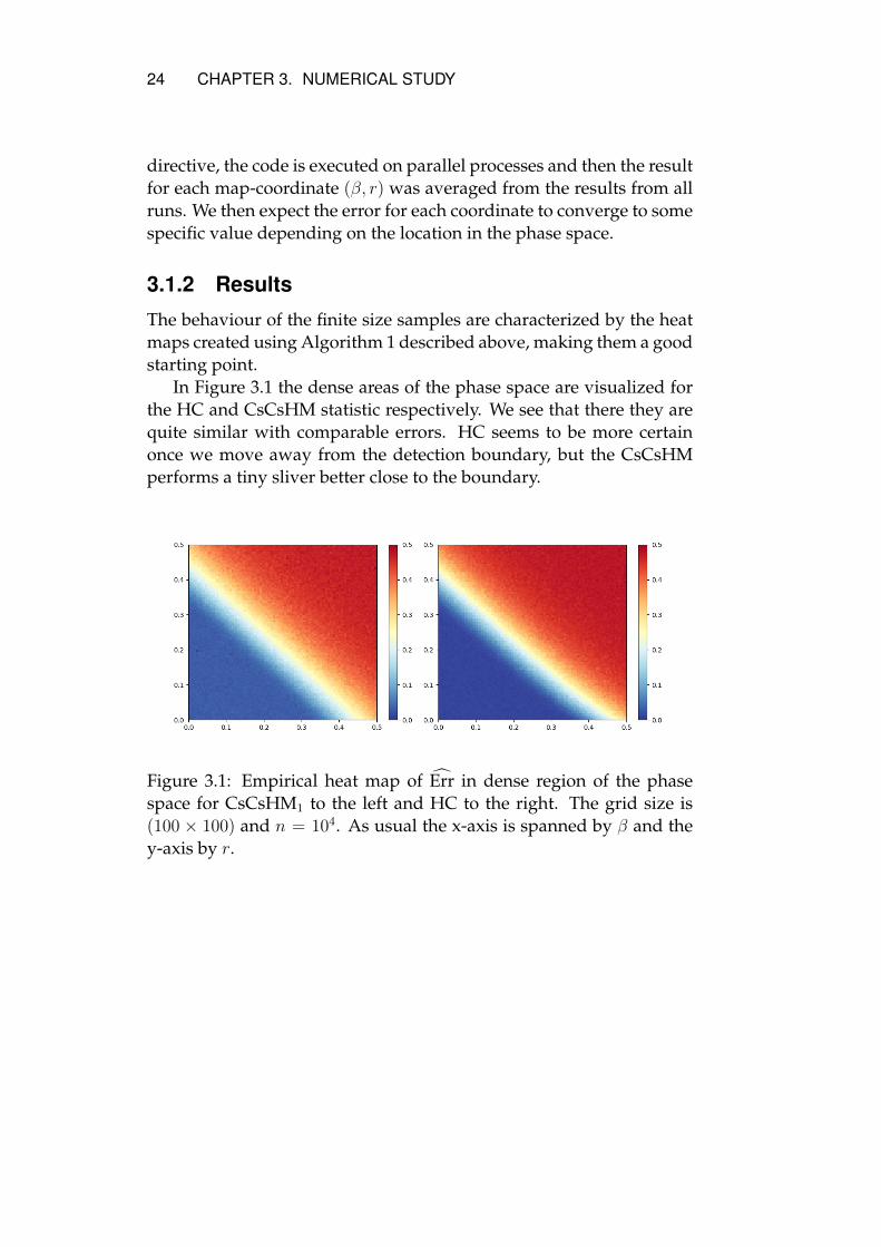
In Figure 3.1 the dense areas of the phase space are visualized forthe HC and CsCsHM statistic respectively. We see that there they arequite similar with comparable errors. HC seems to be more certainonce we move away from the detection boundary, but the CsCsHMperforms a tiny sliver better close to the boundary.

Figure 3.1: Empirical heat map of Err in dense region of the phasespace for CsCsHM1 to the left and HC to the right. The grid size is(100 × 100) and n = 104. As usual the x-axis is spanned by β and they-axis by r.


Figure 3.2: Empirical heat map of Err in sparse region of the phasespace for CsCsHM1 to the left and HC to the right. The grid size is(100 × 100) and n = 104. As usual the x-axis is spanned by β and they-axis by r. Here α0 = 0.1 for CsCsHM and α0 = 0.5 for HC.

Moving on to the sparse heat maps, Figure 3.2, we see that the twostatistics are comparable here as well. Both seem to perform well onceit has some distance to the detection boundary. The HC statistic seemsto be better at weaker signals around β ∈ (0.5, 0.7) but CsCsHM isbetter for larger β:s. This phenomenon remains unexplained. Whatwas noticed when experimenting was that the choice of α0 affectedthe error rates, especially for CsCsHM, with higher α0:s giving muchworse results. HC was more resistant to this behaviour.

To explore the error we look at the test statistics’ values under H0

and H1. In Figure 3.4 we see the behaviour of the HC test variables,and in Figure 3.3 for CsCsHM. For the latter we have removed the thinbut long upper tail of the alternative hypothesis to make the visualiza-tion more clear. Under H0 it seems that CsCsHM has a heavy uppertail, which makes it difficult to separate it from the alternative’s lefttail, which we can see in the bottom picture of the two figures. HC haslighter left tail and is therefore more separable for when H1 or H0 aretrue.


Figure 3.3: Histograms of the CsCsHM1 test statistic for simulateddata. The orange bins correspond to when the alternative H1 is trueand the blue bins when H0 is true. The parameters in the phase spaceare: top left (β = 0.55, r = 0.9), top right (β = 0.9, r = 0.3) and bottom(β = 0.55, r = 0.3).


Figure 3.4: Histograms of the HC test statistic for simulated data. Theorange bins correspond to when the alternative H1 is true and the bluebins when H0 is true. The parameters in the phase space are: top left(β = 0.55, r = 0.9), top right (β = 0.9, r = 0.3) and bottom (β =

0.55, r = 0.3).

3.2 Classification

For classification we want to investigate CsCsHM thresholding through-out the phase space. In addition we want to investigate the perfor-mance on some cancer data sets in comparison to HCT.


3.2.1 Methods

To study the classification we will need an error measure to be able tolook at the finite sample size behaviour of the CsCsHM thresholdingprocedure. To investigate the cancer data sets we need a procedurethat allows us to use the framework without violating our assump-tions too much.

Error measure for the phase diagram

For the classification situation we want to measure the capability ofthe classifier to correctly separate the two classes by selecting the in-teresting variables. A natural way to measure this possibility is to seehow well it performs on a test data set. The error is thus taken as themisclassification rate on a set of data not used in training,

Err =#falsely classified points

#total points. (3.2)

With this error, heat maps spanning over the phase space were plot-ted with the intention to show how the boundary changes close to thetheoretical detection boundary. To do this we generate training andtest data of equal sizes with balanced distribution over classes, trainour classifiers on the training data and finally we apply them on thetest data. The color in the heat map is scaled after the error.

Procedure for the cancer data sets

In order to assess the classification procedures, they were tested onsome real data. The data sets chosen have been explored with varioustechniques, where there are reported error rates for both simple andcomplex classification methods.

Two microarray datasets that have been successfully used for dif-ferentiating patients with cancer and without cancer have been de-scribed by Alon et al [18] and Golub et al [19]. The first is for coloncancer and the second for leukemia. Both Donoho and Jin [4] as wellas Dettling [20] have applied various techniques for classification onthese data sets. The colon cancer data set consists of n = 62 samplesdistributed over the classes as n1 = 40 and n2 = 22 with dimension-ality p = 2000, and the leukemia data set consists of n = 73 samplesdistributed as n1 = 48 and n2 = 25 with dimensionality p = 7129.


It is of course difficult to decide the sparsity β or signal strengthr for the data sets, but the setting is certainly p >> n for these datasets. and the hypothesis is that only a few of the genes’ expressionscorrelate with the disease.

In order to compare the CsCsHM to the HCT approach, both wereapplied to the data sets. The testing procedure was kept simple, form-ing z-scores, using the HC or CsCsHM procedure to find a thresholdvalue to select interesting variables from these, and then finally apply-ing this classifier on a test set not used in training.

Calling the set of all data as the union of the set of data in eachclass, C = C1 ∪ C2, and denoting the size of a set A as |A|, the z-scoresare formed as

z∗j =1√

1/|C1|+ 1/|C2|xj1 − xj2

sj, 1 ≤ j ≤ p, (3.3)

where the standard deviation sj is estimated by

s2j =1

|C| − 2

(∑i∈C1

(xij − xj1)2 +∑i∈C2

(xij − xj2)2)

and the class mean for class k as xji = 1|Ck|∑

j∈Ckxij . Since we do not

know the underlying distribution of the gene expressions, we look atthe difference of the class means which we can expect to be approxi-mately normally distributed.

These scores are then normalized,

Zj =z∗j − z∗

std(z∗), 1 ≤ j ≤ p, (3.4)

where std(z∗) is the standard deviation of the z-scores, and z∗ is theirmean.

Using either the HC or CsCsHM procedures, the threshold value isfound from these scores. This value is used to choose variables, whichare in turn used to classify each sample in a test set. The misclassifica-tion rate was then calculated. To calculate the mean misclassificationrate, a 10-fold cross-validation split of the data was used: the classifierwas trained on 9/10th of the data and tested on the remaining 1/10th.The testing set was rotated so that all parts was used for training andtesting. This was done for three procedures, first HCT with the HC+

statistic as defined in equation 2.22 with the normalization as in HC2008


2.21, then for the alternative CsCsHM thresholding procedure with thetwo statistics CsCsHM1 and CsCsHM2 as found in 2.35 and 2.36.

3.2.2 Results

Heat maps

The heat map, see Figure 3.5, shows that the CsCsHM1 classifier has adecent behaviour in the area just above the detection boundary. As hasbeen noticed before for signal detection, there is no sharp boundary inthe case of classification either. The classifier has a "grey area" for finitesamples where classification is possible, but with a slightly elevatederror rate of roughly 0.25. This area is quite big when β > 0.5. We alsonotice that the plot is quite non-smooth, despite the high number ofsamples, meaning that the results have a high variance.

Figure 3.5: Empirical behaviour of finite sample size of CsCsHM1

thresholding near the detection boundary for classification. Hereθ = 0.4, α0 = 0.1, the grid size is (100× 100) and n = 103.

Cancer data classification

In Table 3.1 and Table 3.2 the results for the classification of the cancerdata sets are presented. As we can see, the statistics behave differently.Although the error is comparable between all three classification pro-


cedures, the number of selected variables varies widely. The CsCsHM2

statistic consistently chooses a lot more variables, while both HC andCsCsHM1 choose fewer depending on the data set.

When looking at the objective function for all the feature scores (ina way similar to what is done in [6]) for the cancer data, we notice thatthey have peculiar s-shapes, see Figure 3.6. For both data sets we seethat the choice of α0 will heavily impact the test statistic. This is not adesirable behaviour since we want the method to be non-parametric.

Figure 3.6: CsCsHM1 objective function for every feature score for thetwo cancer data sets, leukemia to the left, and colon cancer to the right.The x-axis is taken as the fraction of the features (to simplify the inter-pretability of the effect of α0).

Table 3.1: Mean misclassification rates and mean number of variablesselected with standard deviation for the leukemia data set, with a sizeof (73× 7129), for different procedures.

Method Misclassification rate N. variables selectedHC+ 0.024 (±0.00771) 151.4 (±4.35)

CsCsHM1 0.026 (±0.00284) 68.4 (±3.09)

CsCsHM2 0.0246 (±0.00437) 1275.3 (±661.37)


Table 3.2: Mean misclassification rates and mean number of variablesselected with standard deviation for the colon cancer data set, with asize of (62× 2000), for different procedures.

Method Misclassification rate N. variables selectedHC+ 0.1058 (±0.01024) 35.8 (±4.78)

CsCsHM1 0.1075 (±0.01176) 87.6 (±12.30)

CsCsHM2 0.1075 (±0.01115) 137.1 (±22.83)

Investigating the effect of α0

In an attempt to try to understand how many variables are chosen re-lates to the position in the phase space, simulations for different pointswere made. In Figure 3.7 we let r vary over ten points for a fixed β andobserve the behaviour of the error as well as the number of variableschosen. In Figure 3.8 we let β vary instead for a fixed r and observe theresults. What can be noted is that when truncating the upper part ofthe objective functions with a small α0, CsCsHM chooses fewer vari-ables. The error behaves roughly the same.

Looking at Figure 3.8 we can see that for HC the number of vari-ables selected as β is small seems to be the same as the number ofinformative signals. This number decreases as the sparsity increases,only to increase again when the sparsity is so high that the signals arevery few. The same behaviour in reverse can be observed in Figure3.7, where we start with very weak signals so the signals cannot bedifferentiated from the noise. For both images we notice that CsCsHMperforms consistently worse than HC in mean error.


Figure 3.7: Mean error and mean number of selected variables forCsCsHM1 thresholding and HCT for a fixed β = 0.5 on p = 103 di-mensions and varying r for θ = 0.3. To the left: αCsCsHM0 = 0.1 andαHC0 = 0.5 to the right αCsCsHM0 = αHC0 = 1

Figure 3.8: Mean error and mean number of selected variables forCsCsHM1 thresholding and HCT for a fixed r = 0.8 on p = 103 di-mensions and varying β for θ = 0.3. To the left: αCsCsHM0 = 0.1 andαHC0 = 0.5 to the right αCsCsHM0 = αHC0 = 1.

Chapter 4

Discussion

In this section we attempt to explain the results and put them in aproper context. Some suggestions for future work are also proposed.

Remarks and conclusions

The behaviour of the different statistics for finite sample sizes is key tohow useful they are in practice. These initial explorations done in thisreport are a good starting point but it remains to do a more thoroughinvestigation where the connection of the statistics behaviour and theparameter α0 is more precisely mapped out.

Heat maps of the empirical error show that the statistics are compa-rable when it comes to signal detection. The impact of α0 was noted asa big factor for the performance of the CsCsHM type statistics, whichputs them at a disadvantage for practical use. Moreover it seems thatfor classification the HC type statistic manages to select the correct sig-nals to a higher extent, giving the classifier a lower error. However,CsCsHM has a similar error but slightly elevated, and chooses fewervariables. To get a lightweight model with as few variables as possible,one could argue that the easiest way is either using CsCsHM, or usingHC and choosing a subset of the selected variables.

Classification on real data sets is a very practical hands-on way ofcomparing the classifiers, but the exact results are maybe not that inter-esting. Since the data sets are special cases chosen because they havebeen used before, there is nothing new brought to the table and theresults could be circumstantial. This part did contribute to the under-standing the number of variables that are chosen by the statistics.

To sum up, the conclusion is that despite CsCsHM:s better asymp-

34

CHAPTER 4. DISCUSSION 35

totical properties, their performance are still in practice equal to slightlyworse than the HC type statistic for sample sizes up to 104.

Suggestions for future work

Future numerical studies could systematically investigate the CsCsHMstatistics behaviour for different α0:s on simulated data. The impact ofthe sample size should also be more carefully investigated. For classi-fication the number of correctly chosen variables from simulated datacould be taken as a more accurate and interesting measure of perfor-mance than error on a test set. This would also lower the computa-tional cost of the simulations.

In this report we have only considered the normal mixture casewith homoscedasticity, and this is only a special case. There are alot of interesting models including more challenging situations suchas non-gaussianity and heteroscedasticity. Since the CsCsHM statisticwas just recently proposed, there are not a lot of theoretical results inthese areas, but empirical investigations of finite size sample data forHC and other statistics such as Berk-Jones would be interesting.

Bibliography

[1] David Donoho and Jiashun Jin. Higher criticism for detectingsparse heterogeneous mixtures, 2004. ISSN 00905364.

[2] Natalia Stepanova and Tatjana Pavlenko. Goodness-of-fit testsbased on sup-functionals of weighted empirical processes. arXivpreprint arXiv:1406.0526, to appear 2017.

[3] David Donoho and Jiashun Jin. Feature selection by higher crit-icism thresholding achieves the optimal phase diagram. Philo-sophical Transactions of the Royal Society of London A: Mathematical,Physical and Engineering Sciences, 367(1906):4449–4470, 2009.

[4] David Donoho and Jiashun Jin. Higher criticism thresh-olding: Optimal feature selection when useful features arerare and weak. Proceedings of the National Academy of Sci-ences of the United States of America, 105(39):14790–5, 2008.ISSN 1091-6490. doi: 10.1073/pnas.0807471105. URLhttp://www.scopus.com/inward/record.url?eid=2-s2.0-54449086895&partnerID=tZOtx3y1.

[5] Jiashun Jin. Impossibility of successful classification when usefulfeatures are rare and weak. Proceedings of the National Academy ofSciences, 106(22):8859–8864, 2009.

[6] David Donoho and Jiashun Jin. Higher Criticism for Large-ScaleInference: especially for Rare and Weak effects. Statistical Science,30(1):1–25, 2015. ISSN 0883-4237. doi: 10.1214/14-STS506. URLhttp://arxiv.org/abs/1410.4743.

[7] Niclas Blomberg. Higher criticism testing for signal detection inrare and weak models, 2012.

36

http://www.scopus.com/inward/record.url?eid=2-s2.0-54449086895&partnerID=tZOtx3y1

http://www.scopus.com/inward/record.url?eid=2-s2.0-54449086895&partnerID=tZOtx3y1

http://arxiv.org/abs/1410.4743

BIBLIOGRAPHY 37

[8] Yu I Ingster. Minimax detection of a signal for i (n)-balls. Mathe-matical Methods of Statistics, 7(4):401–428, 1998.

[9] Theodore W Anderson and Donald A Darling. A test of goodnessof fit. Journal of the American statistical association, 49(268):765–769,1954.

[10] Amit Moscovich, Boaz Nadler, Clifford Spiegelman, et al. On theexact berk-jones statistics and their p-value calculation. ElectronicJournal of Statistics, 10(2):2329–2354, 2016.

[11] Leah Jager and Jon A Wellner. Goodness-of-fit tests via phi-divergences. The Annals of Statistics, pages 2018–2053, 2007.

[12] Pengsheng Ji and Jiashun Jin. UPS delivers optimal phase dia-gram in high-dimensional variable selection. Annals of Statistics,40(1):73–103, 2012. ISSN 00905364. doi: 10.1214/11-AOS947.

[13] Jiashun Jin and Tracy Ke. Rare and Weak effects in Large-ScaleInference: methods and phase diagrams. arXiv preprint, page 31,2014. ISSN 10170405. doi: 10.5705/ss.2014.138. URL http://arxiv.org/abs/1410.4578.

[14] Trevor Hastie, Robert Tibshirani, and Jerome Friedman. The Ele-ments of Statistical Learning (2nd edition). Springer-Verlag, 2009.

[15] T. Tony Cai, X. Jessie Jeng, and Jiashun Jin. Optimal detection ofheterogeneous and heteroscedastic mixtures. Journal of the RoyalStatistical Society. Series B: Statistical Methodology, 73(5):629–662,2011. ISSN 13697412. doi: 10.1111/j.1467-9868.2011.00778.x.

[16] Tatjana Pavlenko, Anders Björkström, and Annika Tillander. Co-variance structure approximation via gLasso in high-dimensionalsupervised classification. Journal of Applied Statistics, 39(8):1643–1666, 2012. ISSN 0266-4763. doi: 10.1080/02664763.2012.663346. URL http://www.tandfonline.com/doi/abs/10.1080/02664763.2012.663346.

[17] Zheyang Wu, Yiming Sun, Shiquan He, Judy Cho, Hongyu Zhao,and Jiashun Jin. Detection boundary and Higher Criticism ap-proach for rare and weak genetic effects. Annals of AppliedStatistics, 8(2):824–851, 2014. ISSN 19417330. doi: 10.1214/14-AOAS724.



http://www.tandfonline.com/doi/abs/10.1080/02664763.2012.663346

http://www.tandfonline.com/doi/abs/10.1080/02664763.2012.663346

38 BIBLIOGRAPHY

[18] U Alon, N Barkai, D a Notterman, K Gish, S Ybarra, D Mack,and a J Levine. Broad patterns of gene expression revealed byclustering analysis of tumor and normal colon tissues probed byoligonucleotide arrays. Proceedings of the National Academy of Sci-ences of the United States of America, 96(12):6745–6750, 1999. ISSN00278424. doi: 10.1073/pnas.96.12.6745.

[19] T R Golub, D K Slonim, P Tamayo, C Huard, M Gaasenbeek, J PMesirov, H Coller, M L Loh, J R Downing, M A Caligiuri, C DBloomfield, and E S Lander. Molecular classification of cancer:class discovery and class prediction by gene expression moni-toring. Science, 286(5439):531–537, 1999. ISSN 0036-8075. doi:10.1126/science.286.5439.531.

[20] M Dettling. BagBoosting for tumor classification with gene ex-pression data. Bioinformatics (Oxford, England), 20(18):3583–3593,2004. ISSN 1367-4803.

large scale inference under sparse and weak alternatives

Documents