large scale simulation on clusters using comsol 4 · large scale simulation on clusters using...
TRANSCRIPT
Large Scale Simulation on Clusters using COMSOL 4.2
Darrell W. Pepper1
Xiuling Wang2
Steven Senator3
Joseph Lombardo4
David Carrington5
with David Kan and Ed Fontes6
1DVP-USAFA-UNLV, 2Purdue-Calumet, 3USAFA, 4NSCEE, 5T-3 LANL, 6COMSOL
Boston MA, Oct. 13-15, 2011
Outline
Introduction and History
What is a cluster?
Simulation results1. Test problems2. Criteria3. Evaluations
What’s coming
Introduction
History of COMSOL Benchmarking
2007 – 3.4
2009 – 3.5a
2012 - 4.2
Need for HPC
Examine capabilities of COMSOL Multiphysics 4.2 running on a computer cluster
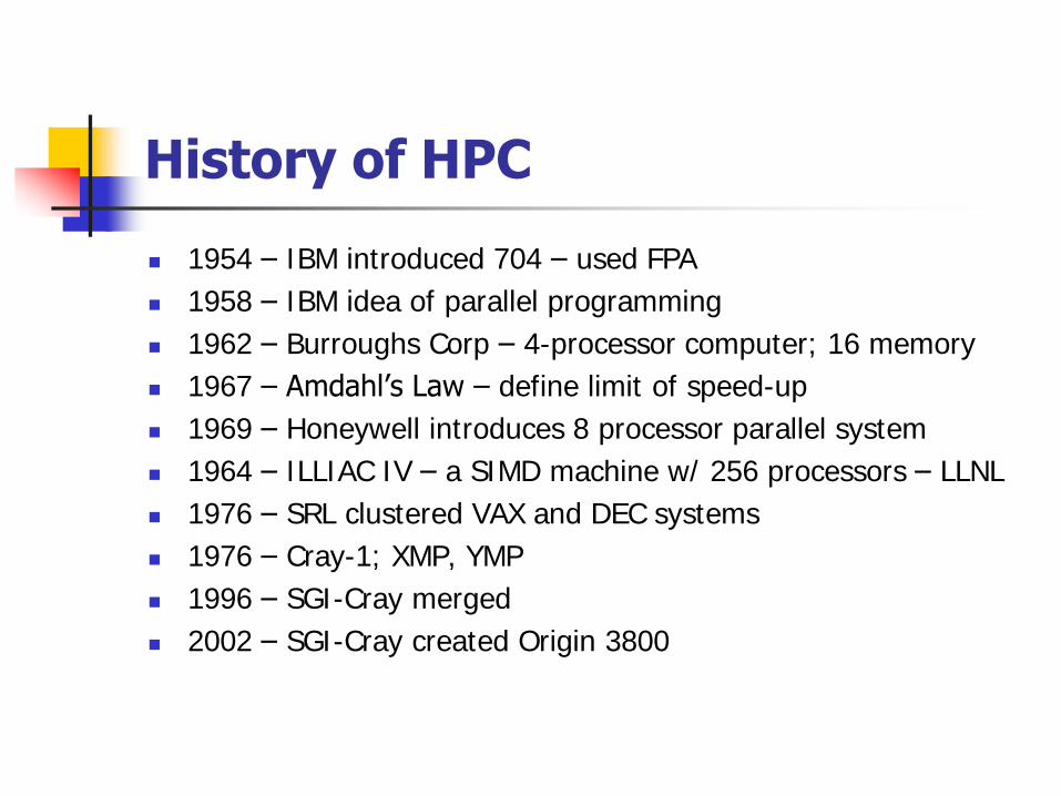
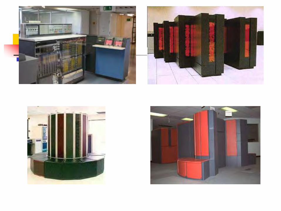
History of HPC
1954 – IBM introduced 704 – used FPA
1958 – IBM idea of parallel programming
1962 – Burroughs Corp – 4-processor computer; 16 memory
1967 – Amdahl’s Law – define limit of speed-up
1969 – Honeywell introduces 8 processor parallel system
1964 – ILLIAC IV – a SIMD machine w/ 256 processors – LLNL
1976 – SRL clustered VAX and DEC systems
1976 – Cray-1; XMP, YMP
1996 – SGI-Cray merged
2002 – SGI-Cray created Origin 3800
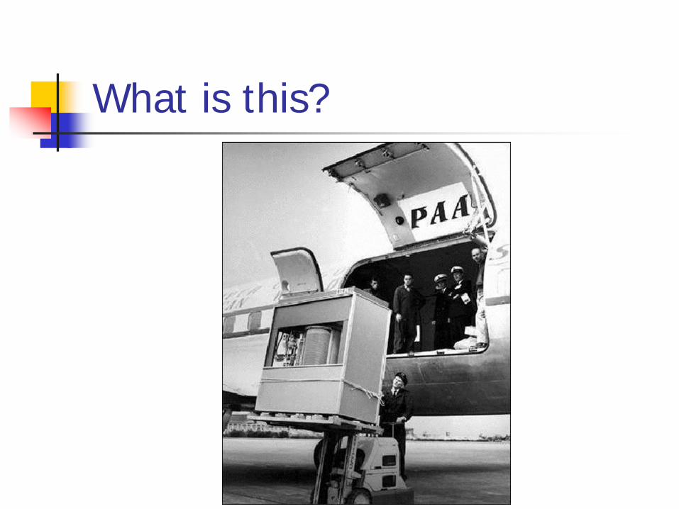
What is this?
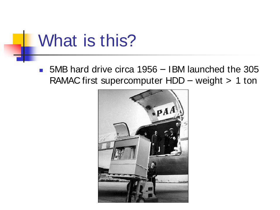
What is this?
5MB hard drive circa 1956 – IBM launched the 305 RAMAC first supercomputer HDD – weight > 1 ton
Computer platform – 4.2 vs 3.5
PC Hardware:
Platform 1: Pentium(R) D CPU 2.80GHz, 4.0GB this configuration was used to test the first four benchmark problems.
Platform 2: Intel ® Core ™ 2 Quad CPU Q9300 CPU 2.50GHz, 4.0GB RAM. This configuration was used for the four CFD-CHT benchmark problems.
Test Problems
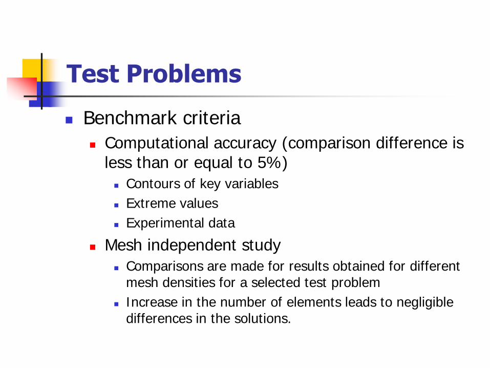
Benchmark criteria
Computational accuracy (comparison difference is less than or equal to 5%)
Contours of key variables
Extreme values
Experimental data
Mesh independent study
Comparisons are made for results obtained for different mesh densities for a selected test problem
Increase in the number of elements leads to negligible differences in the solutions.
Test Criteria
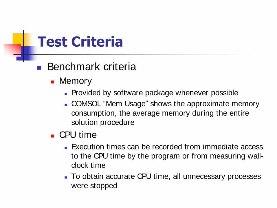
Benchmark criteria
Memory
Provided by software package whenever possible
COMSOL “Mem Usage” shows the approximate memory
consumption, the average memory during the entire solution procedure
CPU time
Execution times can be recorded from immediate access to the CPU time by the program or from measuring wall-clock time
To obtain accurate CPU time, all unnecessary processes were stopped
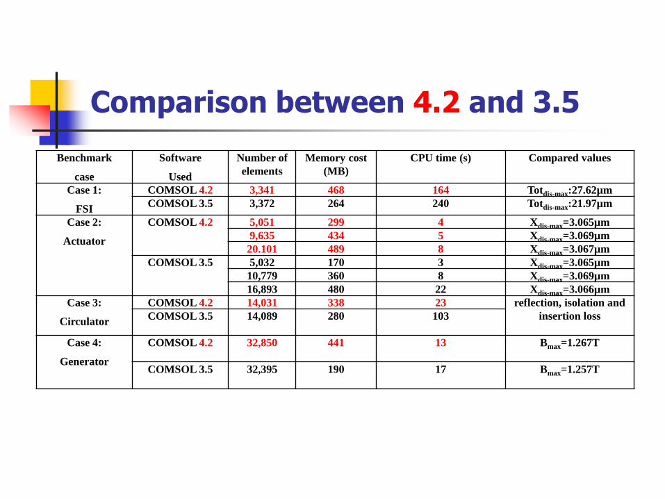
Comparison between 4.2 and 3.5
Benchmark
case
Software
Used
Number of
elements
Memory cost
(MB)
CPU time (s) Compared values
Case 1:
FSI
COMSOL 4.2 3,341 468 164 Totdis-max:27.62µm
COMSOL 3.5 3,372 264 240 Totdis-max:21.97µm
Case 2:
Actuator
COMSOL 4.2 5,051 299 4 Xdis-max=3.065µm
9,635 434 5 Xdis-max=3.069µm
20.101 489 8 Xdis-max=3.067µm
COMSOL 3.5 5,032 170 3 Xdis-max=3.065µm
10,779 360 8 Xdis-max=3.069µm
16,893 480 22 Xdis-max=3.066µm
Case 3:
Circulator
COMSOL 4.2 14,031 338 23 reflection, isolation and
insertion lossCOMSOL 3.5 14,089 280 103
Case 4:
Generator
COMSOL 4.2 32,850 441 13 Bmax=1.267T
COMSOL 3.5 32,395 190 17 Bmax=1.257T
What is a cluster?
A group of loosely coupled computers that work together closely – multiple standalone machines connected by a network
Beowulf cluster – multiple identical commercial off-the-shelf computers connected with a TCP/IP Ethernet LAN
PC Clusters
1994 – first PC cluster at NASA Goddard – 16 PCs – 70 Mflops (Beowulf)
1996 – Cal Tech & LANL built Beowulf clusters > 1 Gflops
1996 – ORNL used old PCs and MPI and achieved 1.2 Gflops
2001 – ORNL was using 133 nodes
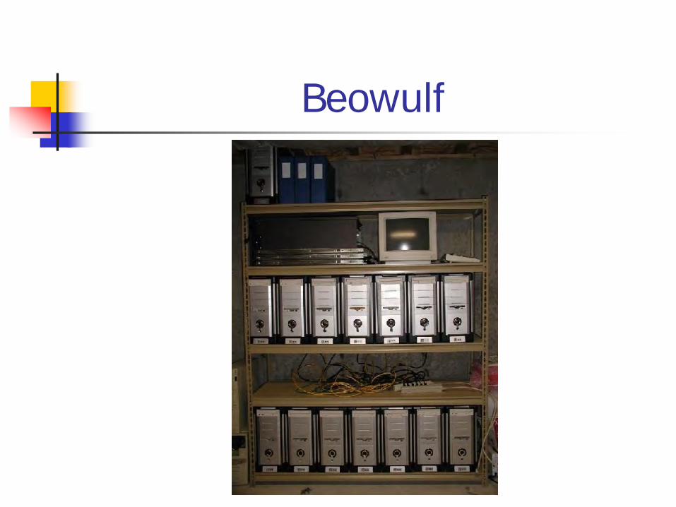
Beowulf
Massively Parallel Processor
A single computer with many networked processors; each CPU contains its own memory and copy of the operating system, e.g., Blue Gene
Grid computing – computers communicating over the Internet to work on a given problem (SETI@home)
SIMD vs MIMD
Single-instruction-multiple-data (SIMD) – doing the same operation repeatedly over a large data set (vector processing – Cray; Thinking Machines –64,000)
Multiple-instruction-multiple-data (MIMD) –processors function asynchronously and independently; shared memory vs distributed memory (hypercube)
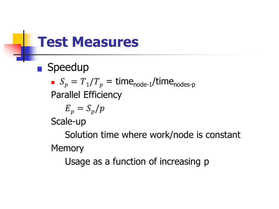
Test Measures
Speedup
Speedup is the length of time it takes a program to run on a single processor, divided by the time it takes to run on multiple processors.
Speedup generally ranges between 0 and p, where p is the number of processors.
Scalability
When you compute with multiple processors in a parallel environment, you will also want to know how your code scales.
The scalability of a parallel code is defined as its ability to achieve performance proportional to the number of processors used.
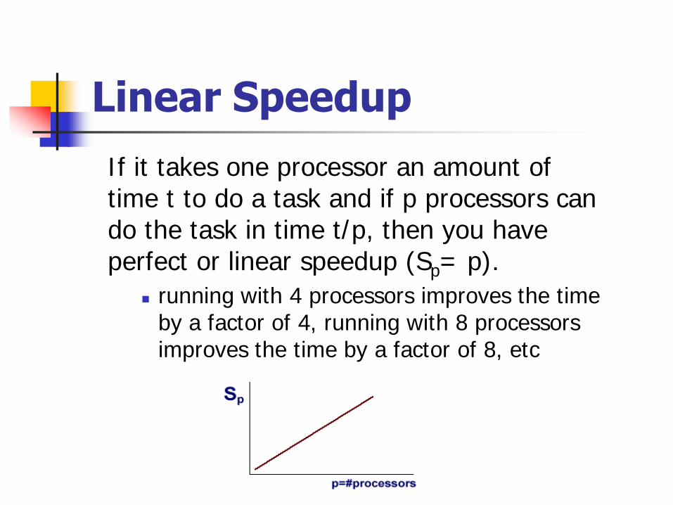
Linear Speedup
If it takes one processor an amount of time t to do a task and if p processors can do the task in time t/p, then you have perfect or linear speedup (Sp= p).
running with 4 processors improves the time by a factor of 4, running with 8 processors improves the time by a factor of 8, etc
Slowdown
When a parallel code runs slower than sequential code When Sp<1, it means that the parallel code runs
slower than the sequential code.
This happens when there isn't enough computation to be done by each processor.
The overhead of creating and controlling the parallel threads outweighs the benefits of parallel computation, and it causes the code to run slower.
To eliminate this problem you can try to increase the problem size or run with fewer processors.
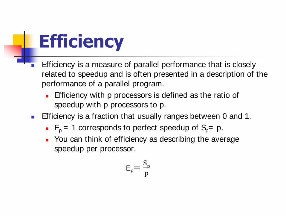
Efficiency Efficiency is a measure of parallel performance that is closely
related to speedup and is often presented in a description of the performance of a parallel program.
Efficiency with p processors is defined as the ratio of speedup with p processors to p.
Efficiency is a fraction that usually ranges between 0 and 1.
Ep = 1 corresponds to perfect speedup of Sp= p.
You can think of efficiency as describing the average speedup per processor.
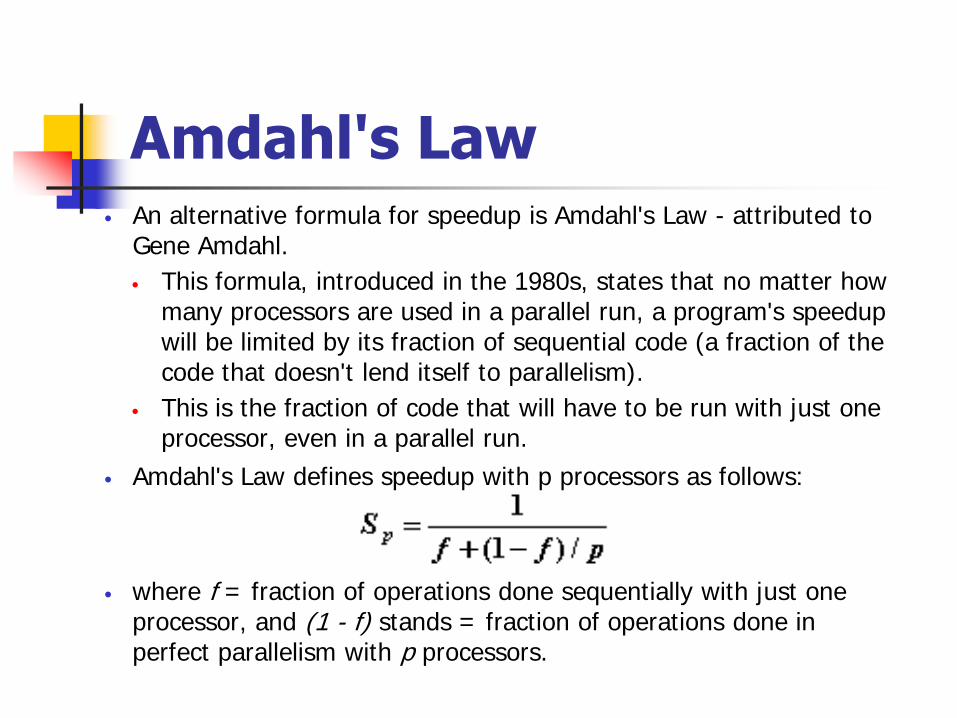
Amdahl's Law An alternative formula for speedup is Amdahl's Law - attributed to
Gene Amdahl.
This formula, introduced in the 1980s, states that no matter how many processors are used in a parallel run, a program's speedup will be limited by its fraction of sequential code (a fraction of the code that doesn't lend itself to parallelism).
This is the fraction of code that will have to be run with just one processor, even in a parallel run.
Amdahl's Law defines speedup with p processors as follows:
where f = fraction of operations done sequentially with just one processor, and (1 - f) stands = fraction of operations done in perfect parallelism with p processors.
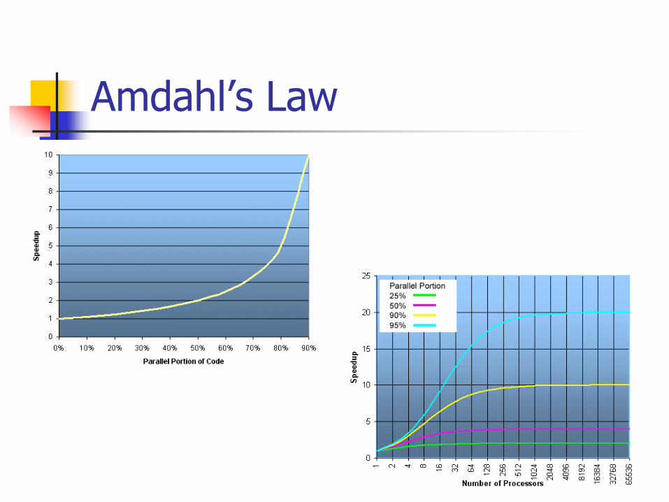
Amdahl’s Law
Amdahl's Law – con’t
Amdahl's Law shows that the sequential fraction of code has a strong effect on speedup
Need for large problem sizes using parallel computers
You cannot take a small application and expect it to show good performance on a parallel computer
For good performance, you need large applications, with large data array sizes, and lots of computation
As problem size increases, the opportunity for parallelism grows, and the sequential fraction shrinks
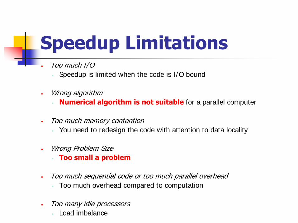
Speedup Limitations Too much I/O
Speedup is limited when the code is I/O bound
Wrong algorithm
Numerical algorithm is not suitable for a parallel computer
Too much memory contention
You need to redesign the code with attention to data locality
Wrong Problem Size
Too small a problem
Too much sequential code or too much parallel overhead
Too much overhead compared to computation
Too many idle processors
Load imbalance
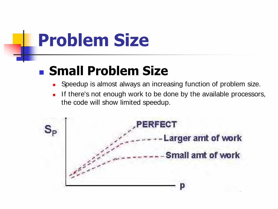
Problem Size
Small Problem Size Speedup is almost always an increasing function of problem size.
If there's not enough work to be done by the available processors, the code will show limited speedup.
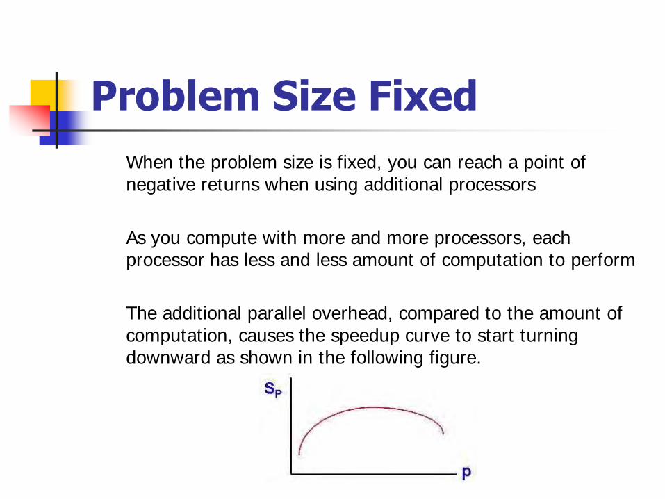
Problem Size Fixed
When the problem size is fixed, you can reach a point of negative returns when using additional processors
As you compute with more and more processors, each processor has less and less amount of computation to perform
The additional parallel overhead, compared to the amount of computation, causes the speedup curve to start turning downward as shown in the following figure.
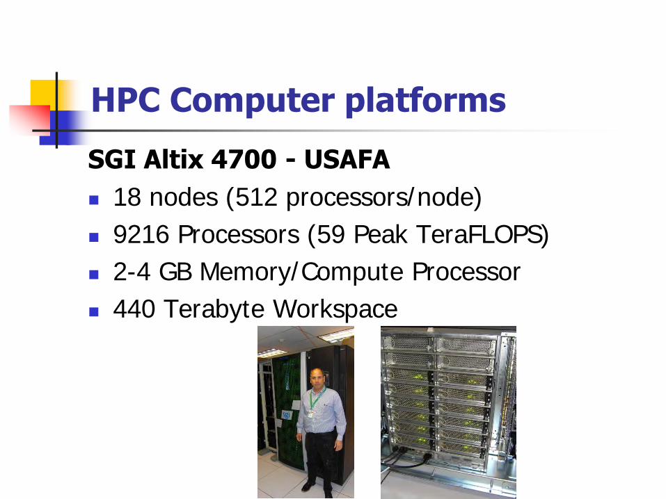
HPC Computer platforms
SGI Altix 4700 - USAFA
18 nodes (512 processors/node)
9216 Processors (59 Peak TeraFLOPS)
2-4 GB Memory/Compute Processor
440 Terabyte Workspace
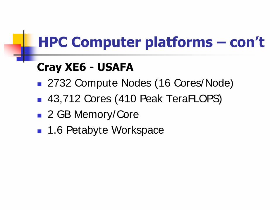
HPC Computer platforms – con’t
Cray XE6 - USAFA
2732 Compute Nodes (16 Cores/Node)
43,712 Cores (410 Peak TeraFLOPS)
2 GB Memory/Core
1.6 Petabyte Workspace

SGI - USAFA
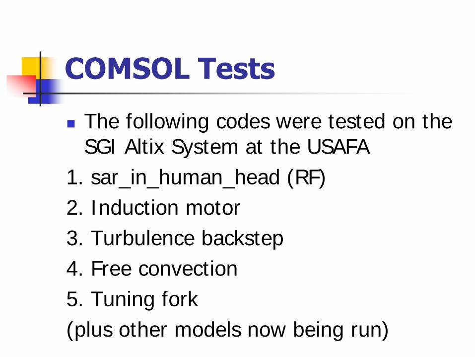
COMSOL Tests
The following codes were tested on the SGI Altix System at the USAFA
1. sar_in_human_head (RF)
2. Induction motor
3. Turbulence backstep
4. Free convection
5. Tuning fork
(plus other models now being run)
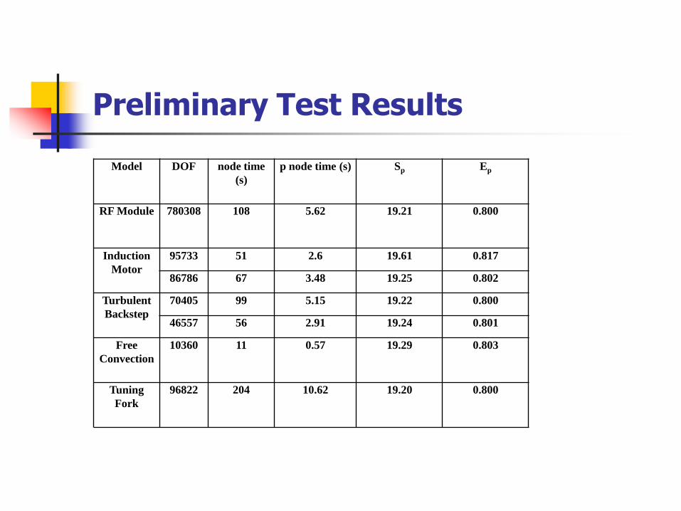
Preliminary Test Results
Model DOF node time
(s)
p node time (s) Sp Ep
RF Module 780308 108 5.62 19.21 0.800
Induction
Motor
95733 51 2.6 19.61 0.817
86786 67 3.48 19.25 0.802
Turbulent
Backstep
70405 99 5.15 19.22 0.800
46557 56 2.91 19.24 0.801
Free
Convection
10360 11 0.57 19.29 0.803
Tuning
Fork
96822 204 10.62 19.20 0.800
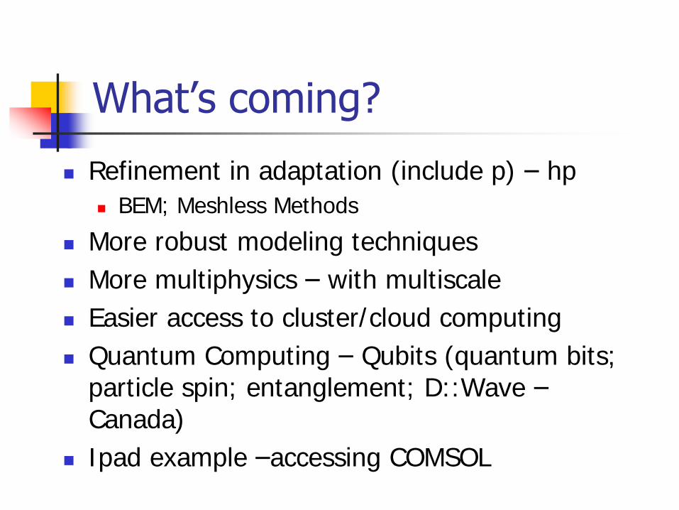
What’s coming?
Refinement in adaptation (include p) – hp
BEM; Meshless Methods
More robust modeling techniques
More multiphysics – with multiscale
Easier access to cluster/cloud computing
Quantum Computing – Qubits (quantum bits; particle spin; entanglement; D::Wave –Canada)
Ipad example –accessing COMSOL
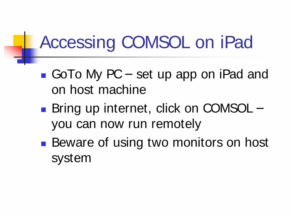
Accessing COMSOL on iPad
GoTo My PC – set up app on iPad and on host machine
Bring up internet, click on COMSOL –you can now run remotely
Beware of using two monitors on host system
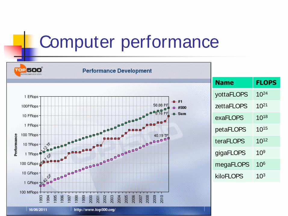
Computer performance
Name FLOPS
yottaFLOPS 1024
zettaFLOPS 1021
exaFLOPS 1018
petaFLOPS 1015
teraFLOPS 1012
gigaFLOPS 109
megaFLOPS 106
kiloFLOPS 103
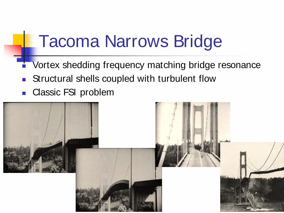
Tacoma Narrows Bridge Vortex shedding frequency matching bridge resonance
Structural shells coupled with turbulent flow
Classic FSI problem

TNB

Contacts
Darrell W. Pepper
USAFA, DFEM, Academy, CO 80840
Dept. of ME, UNLV, NCACM
University of Nevada Las Vegas
Las Vegas, NV 89154
David Kan
COMSOL
Los Angeles, CA