large-scale simulations of turbulent stellar convection - iopscience

Journal of Physics Conference Series

OPEN ACCESS

Large-scale simulations of turbulent stellarconvection flows and the outlook for petascalecomputationTo cite this article Paul R Woodward et al 2006 J Phys Conf Ser 46 370

View the article online for updates and enhancements

You may also likeA kinetic study of the local fieldapproximation in simulations of AC plasmadisplay panelsP J Drallos V P Nagorny and WWilliamson Jr

-

Hierarchical petascale simulationframework for stress corrosion crackingP Vashishta R K Kalia A Nakano et al

-

Mixing and turbulent mixing in fluidsplasma and materials summary of workspresented at the 3rd InternationalConference on Turbulent Mixing andBeyondSerge Gauthier Christopher J KeaneJoseph J Niemela et al

-

This content was downloaded from IP address 201216112231 on 11032022 at 1136

Large-scale simulations of turbulent stellar convection flows and the outlook for petascale computation

Paul R Woodward David H Porter Sarah Anderson Tyler Fuchs

Laboratory for Computational Science amp Engineering University of Minnesota

and Falk Herwig

Los Alamos National Laboratory

paullcseumnedu

Abstract The late stages of stellar evolution have great importance for the synthesis and dispersal of the elements heavier than helium We focus on the helium shell flash in low mass stars where incorporation of hydrogen into the convection zone above the helium burning shell can result in production of carbon-13 with tremendous release of energy The need for detailed 3-D simulations in understanding this process is explained To make simulations of the entire helium flash event practical models of turbulent multimaterial mixing and nuclear burning must be constructed and validated As an example of the modeling and validation process our recent work on modeling subgrid-scale turbulence in 3-D compressible gas dynamics simula-tions is described and a new turbulence model presented along with supporting results Finally the potential impact of petascale computing hardware on this problem is explored

1 Introduction Only a few hundred million years after the Big Bang the earliest stars were formed from gas containing hydrogen helium and only trace concentrations of a few other light elements The heavier elements that make up planets like the earth and on which life is based were generated in stars In order to account for the abundances of these elements we need to understand the processes by which these elements are produced in nuclear reactions in early generations of stars and also how they are then expelled into the interstellar medium Stellar explosions form only a part of this story Much of the heavy element abundance is created in stars that expel their outer envelopes to form planetary nebulae Especially for the earliest generation of such stars both the production of the heavy nuclei and their transport to the circumstellar regions are sensitive to 3-D effects that have not been accurately understood Two cases of quiescent burning are distinguished by the stellas mass massive stars continue burning progressively higher-mass elements in shells until they form an iron core and collapse stars below ~10 Msun will go through H- and He-burning phases and up to C-burning for the most massive cases before they form an electron-degenerate core This core is the pre-formed white dwarf which will be the ultimate endpoint of evolution for low-mass stars Before that final stage is reached burning continues for a long time in shells surrounding the degenerate core At this time the unburned envelope is inflated to giant dimensions filling several hundred solar radii with vigorous turbulent convection These asymptotic giant branch (AGB) stars are the precursors of planetary nebulae and the subject of our interest here

Institute of Physics Publishing Journal of Physics Conference Series 46 (2006) 370ndash384doi1010881742-6596461052 SciDAC 2006

370copy 2006 IOP Publishing Ltd

In general burning of two shells around a degenerate core is unstable The instability in AGB stars produces recurrent He-shell flashes These thermonuclear run-aways drive through their enorm-ous energy generation (up to 108

times the solar luminosity in AGB flashes) vigorous convective mixing layers (see Figure 1) Recurrent and interacting mixing episodes in cycles of convective instability result that eventually lead to conditions favorable for a rich and complex nucleosynthesis of elements AGB stars release these elements through thick cold mass loss outflows as observed for example with the Spitzer space telescope AGB nucleosynthesis provides through recurrent and interlocking mixing episodes associated with the He-flashes the primary production of elements like C N O and many n-heavy isotopes like 13C 22Ne and 2526Mg These stars are able to produce these elements beginning only with primordial H and He and therefore play an important role in the overall production of the heavy elements in the universe The nucleosynthesis depends in many non-linear ways on mixing Mixing determines for some elements which fraction is made in quiescent phases and which fraction is made in explosive environments

In AGB stars we have two different types of convective-reactive events at extremely low metal content One is the H-entrainment into the He-flash convection as shown schematically in orange for the second He-flash in Figure 1 [23] Another one occurs during the dredge-up when the extended convective envelope reaches into the H-free core as a reaction to and immediately after the He-shell flash (indicated after the first He-flash in Figure 1) Any turbulent mixing of H across the convective boundary into the H-free and 12C-rich core will lead to locally very large nuclear energy release which in turn drives convective instability even deeper into the core This hot dredge-up [4] has the properties of a H-flame and the property of this hot mixing and burning interface determines the transport of nuclear processed material into the envelope to be ejected from the star It is also suspected that this mixing is related to the formation of the neutron source 13C for the s-process Both of these events H-mixing and H-entrainment are critical for the chemical and structural evolution of the star These phases of evolution cannot be simulated with existing one-dimensional models

From the above discussion it is clear that the process of turbulent mixing is central to the study of nucleosynthesis in early generations of low mass stars We focus in particular here on the need to understand and quantitatively predict the entrainment of gas containing unburned H fuel into the carbon-rich helium flash convection zone To accurately predict this entrainment we need to simulate the vigorous convection above the helium burning shell in 3D and we must also predict the entrainment of gas at the turbulent shear layer at the top of this convection zone We are beginning to perform 3-D simulations of the convection zone now and of the entrainment and mixing of gases at the top of the convection zone but these are still preliminary From very high resolution simulations of this type we will design and validate simplified statistical models of these phenomena for use in coarsened grid calculations that can be run over the long time scales of the helium shell flash at a reasonable cost How this process of first-principles simulation model design and validation

Figure 1 Time evolution of convective mixing and nuclear burning processes in He-shell flash AGB stars Green regions indicate convectively unstable zones CS is the He-shell flash

convection zone During and at the end of dredge-up H-mixing (purple) into the C-rich intershell material can lead to

formation of the n-source 13C for the s-process (pink shaded region) H-entrainment into the CS leads to a H-ingestion flash convection zone (HIF-CZ) shown schematically in orange for

the second He-flash Adapted from Fig 3 in [1]

371

proceeds is illustrated by the work our team at the LCSE has performed over the last several years on modeling unresolved small-scale turbulent motions in the context of simulations of very high Reynolds number flows with our PPM gas dynamics scheme This work is outlined below

2 Modeling Subgrid-Scale Turbulence We here report recent progress on the design and validation of a new model for unresolved turbulence intended for use in our PPM gas dynamics codes [5-8] This model addresses the need in astrophys-ical problems to treat strongly compressible flows with shocks although it does not as yet incorporate magnetic field effects Our turbulence model does not attempt to alter the dissipative properties of the PPM scheme in any way and is thus distinguished from models such as those of for example Pullin and collaborators [910] or Moin and collaborators [1112] whose models are intended for use with schemes lacking any numerical dissipation or for use in hybrid schemes where standard dissipative compressible flow solvers are used only near shocks Our work has been motivated by our study over many years of compressible convection in stars (cf [13] and references therein) and of the instability of compressible shear layers and jets [1415] and can be applied much more broadly than just to the problem of turbulent mixing in AGB stars that has been discussed above

Numerical methods such as PPM for the Euler equations of inviscid fluid dynamics are designed to produce approximations to the limit of viscous solutions as the viscosity is reduced toward zero Experience with these methods over more than two decades has shown that they can do an excellent job of simulating turbulent astrophysical flows without the addition of any model of unresolved turbu-lence In this respect methods like PPM can be viewed as implicit large eddy simulation or ILES techniques [1617] However analysis of a long series of PPM simulations of various turbulent flows clearly shows that for such flows the PPM technique brings about an enhancement of the velocity power spectrum in the near-dissipation range of wavelengths beginning at about 30 and extending to about 8 grid cell widths Sytine et al [18] showed that enhancement of the near dissipation range spectrum is a feature shared with simulations of the Navier-Stokes equations but for Euler solvers like PPM it is confined to shorter wavelength modes One goal for our turbulence model is to enable us to obtain the correct spectrum for wavelengths above about 8 grid cell widths as we do in non-turbulent and in 2-D flows We do not demand that we obtain the correct power spectrum for shorter wave-lengths since we are unable to compute their phases accurately in any event

The classic eddy viscosity approach to subgrid-scale turbulence modeling introduced by Smagorinsky [19] models the effects of unresolved turbulent motions as a pure dissipation However PPM like other modern Euler methods already has a dissipation carefully tuned for compressible flows We therefore need our turbulence model to transfer some of the energy of modes in the near dissipation range not into heat but into a new energy reservoir the turbulent kinetic energy Eturb From here this energy will either be dissipated into heat or reinjected into the flow as ldquobackscatterrdquo We found a clue of how to do this in our analysis of the 3 TB data set from a large simulation of the Richtmyer-Meshkov instability of a multifluid interface We did this simulation in 1998 in collabora-tion with the ASCI turbulence team at Livermore and with IBM using our simplified PPM code sPPM on a grid of 8 billion cells Our analysis of the data is presented in [20] and [21]

21 Insights from the Richtmyer-Meshkov Simulation Data In analyzing the Richtmyer-Meshkov simulation data we found that the regions where energy is being transferred from large- to small-scale motions are those where the determinant of the deviatoric

symmetric rate of strain tensor 1 22 3 D i j j i ijijS u x u x u is negative Since

the determinant of the tensor is a rotational invariant we can go into a frame in which the tensor is diagonalized and see that the determinant is the product of the 3 eigenvalues Since the deviatoric tensor is traceless these 3 eigenvalues sum to zero The sign of their product is therefore negative when the flow is compressing in one dimension and expanding in the other two This is the kind of flow that results when you clap your hands At high Reynolds numbers such a flow tends to create thin shear layers which subsequently roll up due to Kelvin-Helmholtz instabilities and then the resultant vortex tubes tend to interact to produce turbulence This behavior can be very clearly seen in

372

our simulations of the development and decay of homogeneous turbulence resulting from smooth initial stirring (cf [2223] see also Figure 2 above) The sign of the determinant is positive when the flow is expanding in one dimension and compressing in the other two This is the kind of flow that

373

results when you squeeze a tube of toothpaste to create a jet of fluid In such a flow vortex tubes tend to become aligned and they subsequently tend to merge to form larger structures a phenomenon that can be observed in tornadoes which are relatively stable structures In these flow situations where the determinant is positive energy tends to be transferred from small- to large-scale motions and hence we get backscatter

Our analysis of our simulation data led us to propose [2023] a model for the rate F of forward energy transfer from large to small scales

2 detModel f D turbF AL S C E u where A = ndash 075 and C = ndash 067

Here the overbars denote spatial averaging over a filter volume of linear extent Lf and tildes denote mass-weighted averaging Eturb the small-scale turbulent kinetic energy is defined by 2 turb i i i i iiE u u u u and the subgrid-scale stress tensor ij is defined by

ij i j i j i j i ju u u u u u u u The first term in FModel captures the dependence upon the flow topology as measured by the determinant of the rate of strain tensor We can combine the second term with a term turbE u that also arises in the equation for DEturbDt the time rate of change of the turbulent kinetic energy in the co-moving frame of the filtered velocity field

Figure 2 The distribution of the logarithm of the magnitude of the vorticity in a periodic box of air initially of constant density and pressure and stirred on very large scales with an rms velocity of Mach 1 The simulation was performed with the PPM gas dynamics code on a grid of 20483

cells using a dynamically varying number of CPUs between 80 and 500 over a 25 month period on the Itanium-based TeraGrid cluster at NCSA in 2003 The computation required about 200000 CPU-hours A volume rendering of a diagonal slice through the cubical volume is

shown at times 10 115 and 135 during the transition to fully turbulent flow

374

2 21 12 2

( ) ( )

( )

turb turbj j turb turb j j

i i i i ij j i j j j i ij i j i j

E DEu E E ut Dt

p u p u u u p u p u u u u u

We use our model for F to represent the second term ij j iu on the right in this equation When we

combine the term ( )turb j jE u with the term turbC E u in FModel we see that they correspond to an

effective turbulent pressure q = (23) Eturb that varies upon compression as 53 We validated this = 53 effective equation of state by subjecting our very high resolution homogeneous turbulence

simulation end state to a small amplitude long wavelength standing sound wave perturbation and then extracting the average change in Eturb with changes in specific volume This behavior can be under-stood by considering the 3-D compression of a single line vortex and applying the principle of angular momentum conservation

The grids for our Richtmyer-Meshkov and homogeneous compressible turbulence simulations namely 8 and 86 billion cells are so fine that we can filter the computed results in order to obtain the flowrsquos averaged behavior on much coarser grids as well as values on these coarser grids of quantities like Eturb and ij that depend upon the details of the flow inside each such coarse grid cell The work of Sytine et al [18] indicates that if we consider a cube of 323 cells as our filter box and hence as one coarsened grid cell the largest wavelength disturbances within this filter box should be computed accurately and free of distortion by either direct or indirect effects of PPMrsquos numerical dissipation We would like to construct from our high resolution simulation data results that we might hope some day to be able to obtain with an exceptionally accurate numerical scheme Such a scheme would produce not only cell averaged values of the fundamental physical state variables p u

x u

y and

uz but it would also include a mechanism to estimate the first few terms in the Taylor series expansions of these variables about the center of the cell Obtaining the cell averages volume weighted for the first 2 variables and mass weighted for the velocities in 323 or 643 grid bricks is a simple matter We also evaluate the first 10 moments of these distributions within these volumes and use them to determine the best fit polynomial representation of each variable within the filter volume including all 10 terms up to second order Clearly if we apply this filtering operation once again to the filtered polynomial distribution it has no effect so that the filter is idempotent Using the stand-ard definitions given earlier we can now easily obtain on our coarse grid of filter boxes ij Eturb and all the terms in the equation for DEturbDt We can use this data in two ways First we can test ideas for model equations such as the one given above for F and second we can demand that any model we formulate for unresolved turbulence in a PPM simulation of this coarse grid of this same fluid flow problem must produce results for these quantities that agree well in an appropriate statistical sense with these values obtained from the very high resolution simulation data

Our analysis of our simulation data indicates that the first bracketed term on the right in DEturbDtabove the p-dV work term has little effect and therefore we neglect it Also the effect of the final term which is the divergence of a flux can be modeled by a diffusion of Eturb via

2 2 turb diffuse f turb turbDE Dt C L E E with Cdiffuse

= 007 We know that the action of

viscosity which is omitted from the equation above for DEturbDt must also cause Eturb to decay into heat We observed this behavior especially carefully in our simulation of decaying homogeneous Mach 1 turbulence on a 10003 grid which was run for a very long simulated time If we suppose that the rate at which E

turb decays is proportional to the eddy turn-over time on the scale of our filter then

we get the simple decay model ( ) 2 turb decay turb f turbDE Dt C E L E We find that Cdecay

051 once the shape of the spectrum becomes fully established around time 2 On average this estimate indicates that the local turbulent kinetic energy will persist for about 100 time steps or about a quarter of the time for the turbulence to become fully developed before it has a chance to decay significantly in a simulation of Mach 1 decaying turbulence using a 1283 grid and a value of 4 x for

375

Lf This presents no problem since in our model calculations we always evolve E

turb as an additional

dependent variable We implemented a simple turbulence model (cf [23]) based upon the model ideas described above

in our PPM gas dynamics code In the usual PPM dynamical calculation we included a turbulent pressure q = (23) E

turb along with the normal gas pressure In shock compressions we need to

compute the separate changes in heat and turbulent kinetic energy using their separate equations of state Integrating the conservation laws across the shock in the standard fashion gives us the jump in the sum of the heat and turbulent kinetic energies To estimate how much of this ldquointernal energyrdquo jump should be assigned to Eturb we have been guided by a detailed analysis of simulation data for a Mach 5 shock which we caused to propagate through the fully developed turbulence of the end state of our PPM simulation of decaying homogeneous turbulence on the 20483 grid We treat the gas as a fluid with an effective gamma-law equation of state (cf [7]) The effective gamma is given by

eff = ( p + 5q3) (p+q) The effective Eulerian sound speed is given by c2

eff = ( p + 5q3) The

procedure described in [8] gives us estimates for the time-averaged values of and (p+q) at grid cell interfaces From the density change or jump if we have a shock along the averaged streamline crossing the cell interface we find that we get a reasonable estimate for the change or jump in q by using the shock formula with eff From the jump in q knowing the jump in (p+q) we can then get the jump in p This is not an obvious procedure and we plan to refine it through further shock-turbulence interaction studies but it appears to work rather well It accounts in an approximate way for the large and sudden loss of turbulent kinetic energy to heat immediately following the viscous shock as the turbulence reestablishes local isotropy

Like the heat Eturb

is advected along with the gas in this PPM dynamical step but there are no subgrid-scale turbulence stresses

ij applied in this first PPM step In a subsequent step in which no

fluid motion takes place we first apply the standard PPM test for smoothness of the velocity field (see [8]) yielding an ldquounsmoothnessrdquo indicator function varying from 0 to 1 We also construct a smoothed velocity field by taking for each velocity component half the present value plus a quarter of each neighbor value doing this in the 3 grid directions in succession Where the flow is not smooth we apply the modeled diffusion and decay of Eturb after we first accomplish the energy transfer FModelbetween the resolved velocity field and Eturb via an eddy viscosity proportional to the determinant term in F

Model above evaluated using the smoothed velocity components and set to 0 in shocks

Effectively this procedure sets the shape ndash the relative signs and magnitudes of the 6 independent components ndash of the tensor ij equal to that of the tensor Sij As reported in [23] this turbulence model implementation in PPM gives a computed spatial distribution of Eturb that matches that determined from very high resolution simulation data quite well However we have found that this good behavior is not enough The velocity power spectrum still has an enhancement in the near dissipation range with this approach [30] We therefore seek a better representation of the shape of ij

22 A New Model for the Subgrid-Scale Stress Tensor The analysis of Leonard [24] produces a model for ij whose leading terms produce a contribution to the energy transfer rate F = ij j iu that includes a term in det(SD) This seemed therefore a

good place for us to start in modeling ij as opposed to modeling only F It is easy to derive Leonardrsquos model for ij from a filter of our type but using only the lowest-order moment (the spatial average) in the filter box Within the box the filtered distribution is then a constant rather than a quadratic polynomial We can estimate the leading error in this simplest filtered representation of ui

by taking the leading terms in the Taylor series expansion of ( )iu x y z where the centered and scaled spatial coordinates range from ndash12 to +12 in going over the filter box Then assuming also that we can approximate the derivatives of u

i by those of the filtered velocity we have within the

filter box i i j i ju u x u x Using this estimate and realizing that only terms in even powers

of the coordinates contribute to an average over the filter box we estimate ij as 1 1

12 12 ij i j i j i k j k iju u u u u x u x T

376

With our choice of filter described above based on fitting the 10 low-order moments of the

distribution all the terms in the above estimate for ij are included in both i ju u and i ju u now a

polynomial including terms up to 4th order and therefore cancel and hence should not appear in ij Nevertheless analysis of our high resolution simulation data reveals that the actual values of

ij in

turbulent regions are still fairly well correlated to the expression due to Leonard on the right above The coefficient in front of the bracket is of course no longer 112 We would expect this coefficient to be much smaller since our filter should have captured these Taylor series terms but in fact in turbulent regions the coefficient is actually larger by a factor of about 8 (see [30]) This indicates that the Taylor series is certainly not convergent in these regions in any practical sense and it explains why we must supplement the usual Taylor series approximation of the numerical scheme in such a turbulent region with a turbulence model

From the above discussion we see that Leonardrsquos model for ij in terms of T

ij defined above is a

good candidate to give us the shape of the ij tensor It is not as useful in giving us the magnitude of this tensor since it does not vanish in smooth flow and in other regions the correlation coefficient between ij and Tij varies strongly as a flow goes through the phase of transition to turbulence (see [30]) While the turbulent cascade from large resolved eddies is becoming established and

ij is very

small Leonardrsquos model very greatly overestimates its magnitude The trace of ij is by definition

twice the turbulent kinetic energy Eturb Therefore if we could reliably compute Eturb from an additional differential equation we would have the magnitude of ij and then could model its shape the ratios of its 6 independent components via Tij tr(Tij) Leonardrsquos velocity gradient tensor divided by its trace From a detailed analysis of our high resolution simulation data we find that

ij contains a

component with the shape of Tij as well as one with the shape of Sij (see [30]) The component proportional to Sij increases relative to the other component as the turbulence becomes well developed We find however that in implementing such a model for ij in our PPM code we can leave out the term in S

ij since it is strictly dissipative and is thus redundant in function with the native

numerical dissipation of the PPM scheme From the above arguments a model for the subgrid-scale stress tensor ij emerges

( )D turb D ijij ijE T tr T where 2 jiij f

k k

uuT Lx x

4fL x and 45

Here TD is the deviatoric part of the tensor Tij because the above model is only for the deviatoric part of ij the tensor D We treat the remainder of ij together with the pressure as we have described earlier In the expression for Tij we have dispensed with the scaled coordinates kx in order to emphasize the dependence upon Lf the width of the filter box This constant cancels out of the above expression for ij but it enters non-trivially in the differential equation we must solve to evolve Eturb Since in the course of a computation we do no explicit filtering we might expect this conceptual filter box width to be x the width of a grid cell By visually comparing the results of a PPM simulation with those of a very much higher resolution simulation that has been filtered with a series of filter sizes we find that the effective filter width of the PPM scheme to the extent that such a quantity is meaningful lies between 3 and 4 grid cell widths and it appears to be closer to 4 than to 3 (see [30] and also Figure 3c and 3d) For use of this model in PPM we therefore choose Lf = 4 x For we choose that value that just eliminates the enhancement of the velocity power spectrum in the near dissipation range for decaying homogeneous turbulence This value turns out to be = 45

It remains to describe how we compute Eturb We follow the procedure we described earlier using the above model for ij We enforce at each grid cell the constraint that energy cannot be taken from Eturb and placed into the resolved velocity field unless we have at that location sufficient energy in Eturb

to extract Thus we explicitly enforce conservation of total energy at each grid cell and this prevents the model from predicting an explosion of kinetic energy from over-draining of the turbulent kinetic energy reservoir Such explosions are a danger with models that predict E

turb from the resolved flow

field at each point in space and time because in such models inverse energy transfer does not reduce and can actually increase the predicted amount of turbulent energy available The above discussion

377

lays out how we evolve Eturb

but it dodges the question of where Eturb

originally comes from If we were to know Eturb at some particular time and if we are modeling the shape of the ij tensor correctly then so long as the magnitude of ij is correct in our model we should get the evolution of Eturb correct as long as we are solving the right dynamical equation for it We see that this equation predicts exponential growth of E

turb so long as the resolved velocity gradients persist to support that

growth If we seed the growth of Eturb then we can expect it to rapidly grow to a saturation value determined by the energy in the smallest resolved scales of motion The growth of Eturb feeds on the energy arriving at these scales due to the turbulent cascade of the resolved flow Eturb thus grows until it exhausts this source of energy This limit to its growth is determined by the resolved flow which is accurately computed Once Eturb reaches this saturation level it should therefore evolve in a manner that is independent of how we seeded it

Our Richtmyer-Meshkov instability simulation data gives us the key to a mechanism to seed the flow with E

turb we should create it in small seed quantities where det(S

D) is large and negative We

can do this easily by adding to our model for ij an eddy viscosity term where the eddy viscosity is some constant coefficient multiplied by ndashdet(SD) properly normalized The results should be fairly independent of our choice of so long as it is small Experimenting with this model using a PPM simulation of an isolated perturbed shear layer on a grid of 10242 512 cells we find that = 001 works very well and = 0001 works well also but produces a short delay in the rise of the average value of Eturb to the correct saturation value in this problem Setting = 01 however begins to compete with our model for

ij in terms of T

ij and hence results in too much damping of modes in

the near dissipation range of the velocity power spectrum Our model equations thus become

i

i

ut x

ij i j D iji

j

p q u uut x

j

j

u E p qEt x

25 3 33 2

i ii D diffuse f decayij

i i j f

q q u u q qu q C L q Ct x x x L

3 11 2 2 j jpE q u u

1 12 3

jiij D ij ij kkij

j i

uuS S S Sx x

2 1 43

jiij f D ij ij kk fij

k k

uuT L T T T L xx x

007 051diffuse decayC C

2675 det 001D Dij ij

D f Dijkk D Dlm lm

T Sq L ST S S

and 0 in smooth flow

These model equations are solved in the PPM code in the two-step process outlined earlier The test for smooth flow which determines whether or not we let be non-zero is of the standard PPM type (see [8]) comparing the relative magnitudes of the third and first derivatives of the velocity compon-ents In constructing the tensors S and T we also use smoothed velocity components as described earlier In these equations we have eliminated the variable Eturb in favor of (32) q Shocks are treated specially as described earlier

23 First Validation Tests of the New Model for Subgrid-Scale Turbulence In Figure 3a we show the velocity power spectra for PPM simulations of the Mach 1 decaying turbulence problem carried out on 2563 grids with and without the turbulence model The initializa-tion of this problem is similar to that used in Sytine et al (2000) but with an initial rms Mach number of unity rather than of frac12 For comparison the spectrum from the run on the 20483 grid is also shown These are compensated spectra so that the Kolmogorov trend is horizontal The enhancement of the power spectrum in the near dissipation range is clearly evident for the runs without the turbulence model and it is clearly absent for the run with the model At this time namely 2 flow-through times

378

of the energy containing scale the turbulence is well developed and decaying without further change in the shape of the power spectrum [30] In Figure 3b power spectra at time 186 are shown for runs with the turbulence model on grids of 1283 and 2563 cells and again the 20483 spectrum is shown for comparison Clearly the model has eliminated the false enhancement of the near dissipation range spectrum while leaving the dissipation properties of the PPM scheme which for compressible flows are a very positive feature essentially unchanged We expect that this turbulence model will work equally well with any standard modern scheme for the Euler equations In Figure 3c the difficulty of assigning an effective filter width to the PPM scheme is shown The velocity power spectra are shown at time 186 for the PPM 2563 run and are compared with the spectra for the 20483 run unfiltered and filtered over cubical boxes of 83 163 243 323 483 and 643 cells In Figure 3d the PPM simulation with the turbulence model on the 2563 grid is compared to this same series of filtered spectra The member of this series with the same Nyquist frequency has a filter width of 2 of the cells of the 2563

grid The Nyquist frequency is nevertheless the same since the filter has been placed at intervals of half a filter width in order to yield a smoother result At least as far as the power spectrum is concern-ed the PPM run with the turbulence model is quite competitive with the high resolution solution filtered on boxes of just 2 of its cells on a side It would seem unreasonable to expect more

Velocity power spectra represent integrated quantities since the vast complexity of this developed turbulent flow has been condensed into a single line on a plot A comparison of the flow visualiza-tions in configuration space is a far more demanding validation test In Figure 4 we display volume renderings of the same slice of the problem domain at time 11 in the Mach 1 decaying turbulence problem a point about midway through the transition to fully developed turbulence [30] All these

Figure 3 Comparison of compensated velocity power spectra for the Mach 1 decaying homogeneous turbulence problem See discussion in text

d

t = 186

a b

c

PPM 256

PPM2048

PPMturb 256

t = 20 t = 186

PPMturb 128

PPMturb 256

PPM 2048

t = 186

PPM 256 PPM 2048 PPM 2048

PPMturb256

379

slices are rendered in an identical fashion showing the distributions of the logarithm of the vorticity magnitude so that they can be compared on an equal footing At the top left in the figure the unblended results for the 20483 grid are shown Directly below this image panel the results of running PPM on this problem with the turbulence model on a grid of 2563 cells are shown At the top and bottom right are shown respectively the results of filtering the 20483 data over boxes the size of 3 and 4 grid cell widths of the 2563 simulation The model computation produces a result whose quality is intermediate between these two filtered results and the phases of the modes affected by the model appear to be quite accurate At time 186 the phase agreement is less compelling which is not surprising but the general distribution produced by the model run is intermediate between the high resolution data filtered over boxes of 2 and 3 grid cell widths (see [30]) a result that is consistent with the appearance of the power spectra in Figure 3

We can also validate our turbulence model by testing to see if the distributions of the turbulent kinetic energy Eturb that it evolves agree with those obtained by filtering very much higher resolution PPM simulations In Figure 5 we present on the left such distributions of Eturb as computed on a coarse grid of 1282 64 cells and in the middle of the figure we present the distributions obtained using filter boxes of 323 cells with data from a PPM simulation of the same isolated shear layer problem on a grid of 10242times512 cells At the right in Figure 5 we show the corresponding distribu-tions on the fine grid of the magnitude of the vorticity These displays are shown at times 2 3 4 and 5 sound crossing times of the spanwise extent of the shear layer This numerical experiment was constructed to clarify the role of det(S

D) in the energy transfer rate to small-scale turbulence A

shear layer in air separating Mach 05 flows in opposite directions was set up as initially flat and sinusoidal perturbations in modes 1 2 and 3 were introduced in the velocity component perpendicular to the initial shear layer Above and below the layer counter-rotating circulating flows were set up with velocities up to Mach 025 and with an initially incompressible flow field (see [30]) The

Figure 4 Comparison of vorticity structures for the decaying homogeneous turbulence problem

380

pressure was adjusted to initially balance the centrifugal forces in the counter-rotating circulating flows The shear layer is thus squeezed by the counter-rotating flows on one edge the near edge in Figure 5 and it is being pulled apart along the far edge Along the near edge of the shear layer det(SD) is negative and we should see transfer of energy to small-scale turbulence but along the far edge the transfer of energy should go the opposite way We must remember that the large-scale flow is moving from the near to the far edge of the shear layer and this will carry the turbulent energy along with it The effects of these opposite signs of the energy transfer are clearly evident in the visualizations of the vorticity

Figure 5 Comparison of turbulent kinetic energy structures for the Mach 05 shear layer problem described in the text At the left is Eturb as computed from the turbulence model on a grid of 1282 64

cells in the middle is Eturb obtained by filtering the results of the PPM simulation on a grid of 10242 512 cells At the right is the magnitude of the vorticity for the fine grid PPM run

381

Figure 6 Comparison of the distributions of Eturb averaged in planes oriented perpendicular to the spanwise direction in the isolated shear layer problem of Figure 5

At time 2 the flow is not turbulent at all although Tij is relatively large along the layer and particularly large in the cores of the 3 organized rolls Our filtering procedure reveals that values of the turbulent kinetic energy half the trace of

ij are quite small in these rolls because we have

constructed our filter to capture large-scale structures accurately At this time the traces of ij and T

ij

are correlated but the first is largest on the portions of the thin almost flat shear layer that can be seen breaking up into small vortex tubes while the second is largest in the cores of the large well organ-ized rolls At time 5 when the turbulence is well developed in the two large rolls the distributions of the traces of these two tensors are much more closely alike but the ratio of their magnitudes has changed by a factor of 14 from its average value at time 2 [30] In this flow therefore Tij is a good predictor of the shape of ij but not of its magnitude A more quantitative comparison of the values of Eturb in 323 filter boxes and those predicted by our turbulence model running on a grid of 1282 64 cells is shown in Figure 6 (see also [30]) Here line plots show the variation in the spanwise dimen-sion of averages taken in planes for this flow at 2 of the 4 times shown in Figure 5

The turbulence model we have proposed here shares a number of features with earlier work We have used high resolution direct simulations of turbulent flows to derive the several dimensionless constants that occur in our formulae and to validate in these particular flows our choice of functional forms This approach was pioneered by Clark Ferziger and Reynolds [25] but we have enjoyed the substantial benefits of todayrsquos very much more powerful computing platforms and we have exploited the ability of Euler codes to converge more rapidly to the infinite Reynolds number limit than Navier-Stokes simulations Many other investigators following Leonard have used the square of the velocity gradient tensor to model the subgrid-scale stress including Clark Ferziger and Reynolds [25] and Liu et al [26] but as discussed in Vreman Geurts and Kuerten [27] difficulties were encountered with instability due to backscatter Vreman Geurts and Kuerten [28] modified the Clark model by adding a dynamic eddy viscosity term and this removed the need for a limiter to achieve stability A similar approach is taken by Winckelmans et al [29] In our work we address this stability issue by evolving the turbulent kinetic energy through an additional differential equation and then by strictly enforcing total energy conservation on a cell-by-cell basis We also employ the shape of the square of the velocity gradient tensor but not its magnitude to model

ij This approach demands the seeding of the

turbulent kinetic energy via the small term we include in ij proportional to the determinant of the deviatoric rate of strain tensor Comparisons of different model equations for ij with filtered results of very high resolution PPM simulations indicate that this use of Eturb to obtain the magnitude of ij is superior to the use of any particular constant coefficient multiplied by either T

ij or S

ij or even the

best combination of the two (see [30])

Spanwise distribution of Eturb t= 5

Model

Blended High- Resolution Data

Model



382

3 Outlook for Petascale Computation The above outline of the process by which we have designed and validated our new turbulence model for use in our PPM code (or in any standard Euler code) is intended to illustrate how careful computer simulations if performed on very high resolution grids using governing equations that capture all the necessary physics can play the role traditionally assigned in the scientific method to experiments This does not mean that experiments are obsolete But in many instances like the homogeneous compressible turbulence case discussed above simulations can give us far more detailed data than present experimental techniques We still need to validate our work against experiments but the sparse data they usually provide cannot guide our model construction in nearly the detail that is illustrated by the above example

Our example of homogeneous turbulence is perhaps the simplest one we could presently introduce To design and validate models of the turbulent entrainment and mixing of unburned hydrogen gas at the top of the convection zone in an AGB star would require much more difficult multifluid simulations To design and validate models of nuclear flame propagation in such a turbulent fluid would involve still more detailed and costly computations The 86 billion cell PPM simulation of decaying Mach 1 turbulence was run on NCSArsquos Teragrid cluster in 2003 using between 80 and 500 CPUs over a period of 25 months The total computation time was about 200000 CPU-hours and the computational rate achieved averaged around 13 Tflops Petascale computation thus offeres about a 3-order-of-magnitude increase in computing power over this level Since the computing time in CPU-hours scales as the linear grid resolution raised to the 4th power this increase would allow us to refine the grid in such a simulation by a factor of about 6 in each spatial dimension and time We could use this increase in resolution to simulate at equivalent levels of detail a more complex fluid dynamical process such as a complete section of the AGB starrsquos convection zone or an advancing nuclear flame We could also use some or all of the thousand-fold increase in computaitonal speed to simulate more complex microscopic processes such as elaborate nuclear reaction networks Regardless of how we use this coming petascale computing power we will not be able to avoid the need for modeling small-scale processes such as turbulence Simulating the entire AGB star convection zone through the entire year-long extent of a single helium shell flash even at a sustained petaflops would still take over a year if we were to insist upon a first-principles compuation without resort to modeling

4 Acknowledgements This work has been supported through grant DE-FG02-03ER25569 from the MICS program of the DoE Office of Science Equipment used in the work has been supported by NSF CISE RR (CNS-0224424) and MRI (CNS-0421423) grants a donation of an ES-7000 computer from Unisys Corp and local support to the Laboratory for Computational Science amp Engineering (LCSE) from the University of Minnesotarsquos Digital Technology Center and Minnesota Supercomputer Institute The large simulation of homogeneous compressible turbulence was performed on the NSF TeraGrid cluster at NCSA and some of the slip surface simulations have been performed at the Pittsburgh Supercomputing Center Falk Herwig is supported through the LANL LDRD program

References [1] Herwig F ldquoEvolution of Asymptotic Giant Branch Starsrdquo Annual Rev Astron Astrophys 43

111-1145 (2005) [2] Fujimoto M Y Y Ikeda and I Iben ldquoThe origin of extremely metal-poor carbon stars and the

search for population IIIrdquo Astrophys J Lett 529 L25 (2000) [3] Suda T et al ldquoIs HE0107-5240 a primordial star The characteristics of extremely metal-poor

carbon-rich starsrdquo Astrophys J 611 476 (2004) [4] Herwig F ldquoDredge-up and envelope burning in intermediate mass giants of very low

metallicityrdquo Astrophys J 605 425 (2004) [5] Woodward P R amp P Colella J Comput Phys 54 115 (1984) [6] Colella P amp P R Woodward J Comput Phys 54 174 (1984)

383

[7] Woodward P R in Astrophysical Radiation Hydrodynamics eds K-H Winkler amp M L Norman Reidel 245 (1986)

[8] Woodward P R 2005 ldquoA Complete Description of the PPM Compressible Gas Dynamics Schemerdquo LCSE internal report available from the main LCSE page at wwwlcseumnedushorter version to appear in Implicit Large Eddy Simulation Computing Turbulent Fluid Dynamics ed F Grinstein L Margolin and W Rider Cambridge University Press (2006)

[9] Misra A amp D I Pullin Physics of Fluids 9 2443 (1997) [10] Kosovic B D I Pullin amp R Samtaney Physics of Fluids 14 1511 (2002) [11] Mahesh K S K Lele amp P Moin J Fluid Mech 334 353 (1997) [12] Mahesh K G Constantinescu amp P Moin J Comput Phys 197 215 (2004) [13] Woodward P R Porter D H and Jacobs M ldquo3-D Simulations of Turbulent Compressible

Stellar Convectionrdquo Proc 3-D Stellar Evolution Workshop Univ of Calif Davis IGPP July 2002 also available at wwwlcseumnedu3Dstars

[14] Bassett G M amp P R Woodward J Fluid Mech 284 323 (1995) [15] Bassett G M amp P R Woodward Astrophys J 441 (1995) [16] Margolin L G amp W J Rider Intl J Num Meth Fluids 39 821 (2002) [17] Grinstein F L Margolin and W Rider eds 2006 in press Implicit Large-Eddy Simulation

Computing Turbulent Fluid Dynamics Cambridge Univ Press [18] Sytine I V D H Porter P R Woodward S W Hodson amp K-H Winkler J Comput Phys

158 225 (2000) [19] Smagorinsky J ldquoGeneral circulation experiments with the primitive equationsrdquo Mon Weather

Rev 91 99 (1963) [20] Woodward P R Porter D H Sytine I Anderson S E Mirin A A Curtis B C Cohen

R H Dannevik W P Dimits A M Eliason D E Winkler K-H amp Hodson S W in Computational Fluid Dynamics Proc of the 4th UNAM Supercomputing Conference Mexico City June 2000 eds E Ramos G Cisneros R Fernaacutendez-Flores amp A Santillan-Gonzaacutelez World Scientific (2001) available at wwwlcseumnedumexico

[21] Cohen R H Dannevik W P Dimits A M Eliason D E Mirin A A Zhou Y Porter D H amp Woodward P R Physics of Fluids 14 3692 (2002)

[22] Woodward P R Anderson S E Porter D H and Iyer A ldquoCluster Computing in the SHMOD Framework on the NSF TeraGridrdquo LCSE internal report April 2004 available on the Web at wwwlcseumneduturb2048

[23] Woodward P R Porter D H Anderson S E Edgar B K Puthenveetil A amp Fuchs T 2005 in Proc Parallel CFD 2005 Conf Univ Maryland May 2005 available at wwwlcseumneduparcfd

[24] Leonard A Adv Geophys 18 237 (1974) [25] Clark R A J H Ferziger amp W C Reynolds J Fluid Mech 91 1 (1979) [26] Liu S C Meneveau amp J Katz J Fluid Mech 275 83 (1994) [27] Vreman B B Geurts amp H Kuerten J Fluid Mech 339 357 (1997) [28] Vreman B B Geurts amp H Kuerten Theor Comput Fluid Dyn 8 309 (1996) [29] Winkelmans G S A A Wray O V Vasilyev amp H Jeanmart Phys Fluids 13 1385 (2001) [30] Woodward P R D H Porter S E Anderson T Fuchs amp F Herwig ldquoLarge-Scale

Simulations of Turbulent Stellar Convection and the Outlook for Petascale Computationrdquo PowerPoint slides from SciDAC2006 conference presentation (June 2006) available at the SciDAC2006 Web site and also at wwwlcseumneduSciDAC2006

384

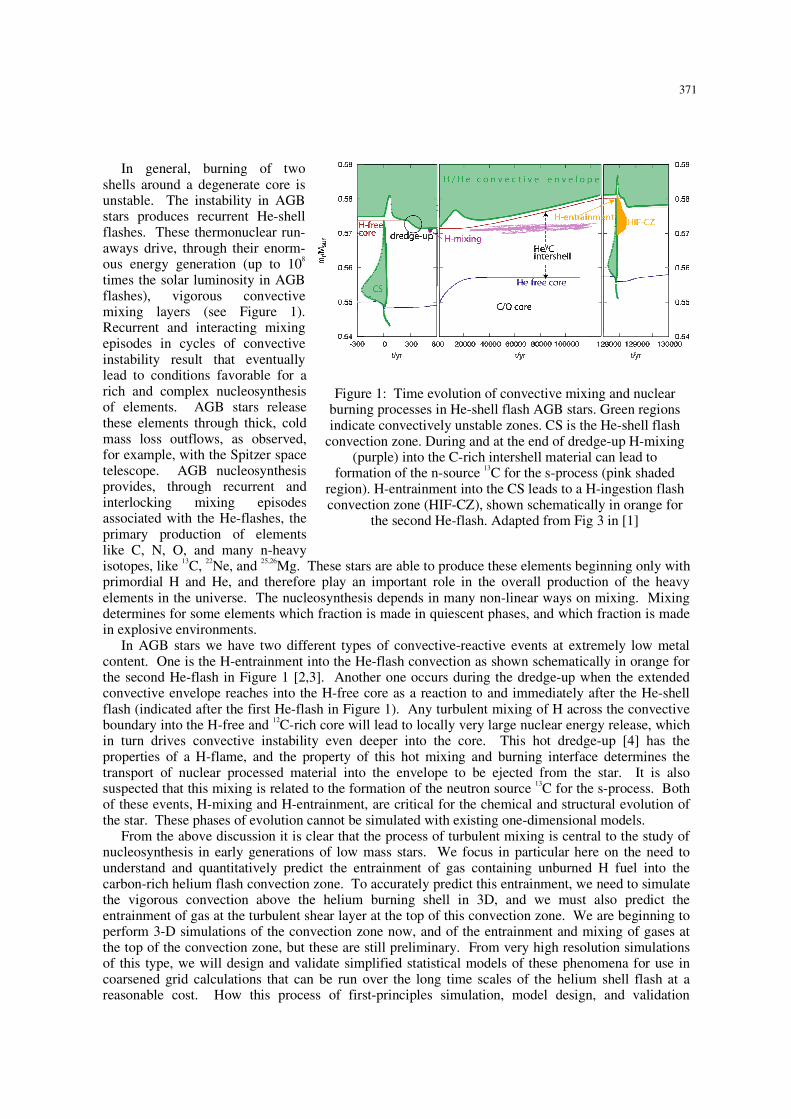
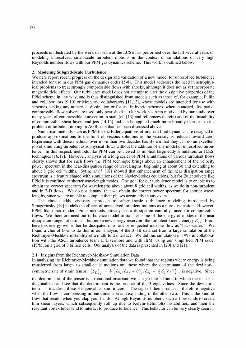
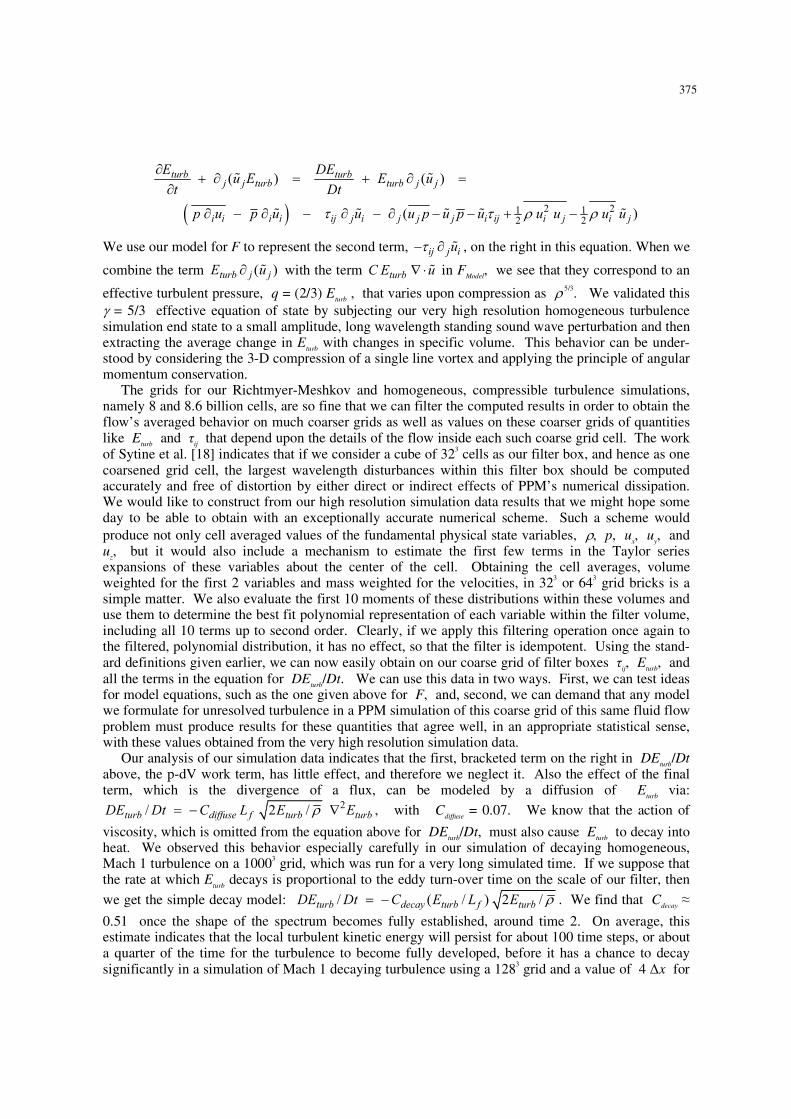
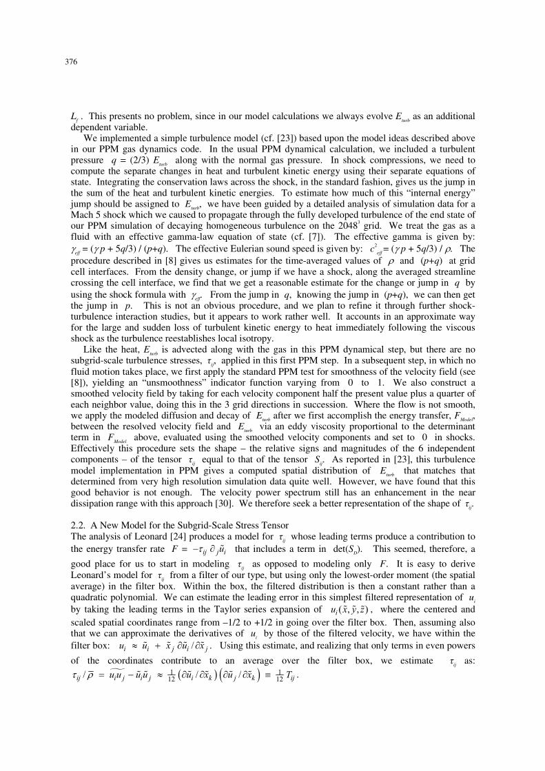
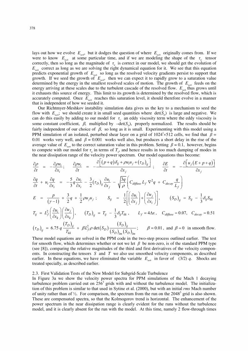
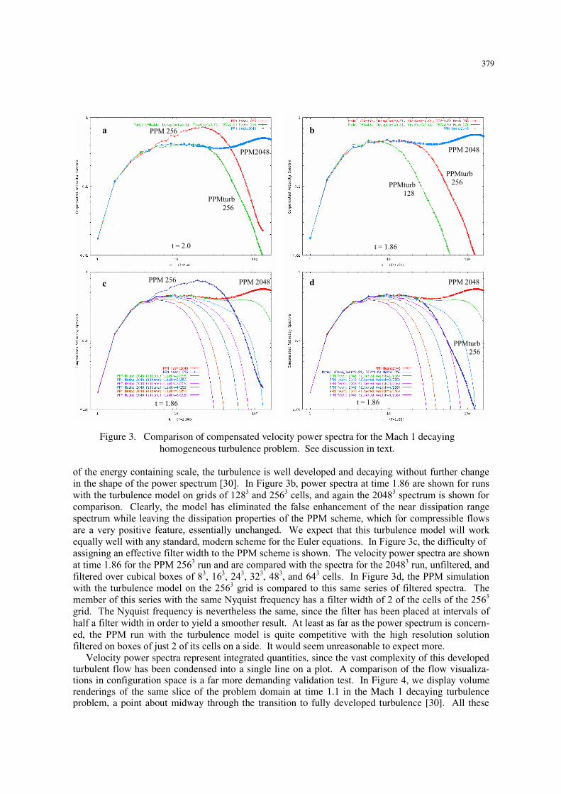
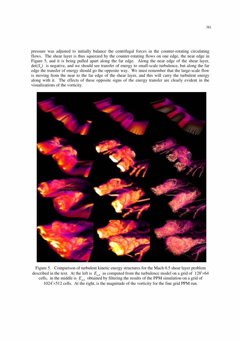
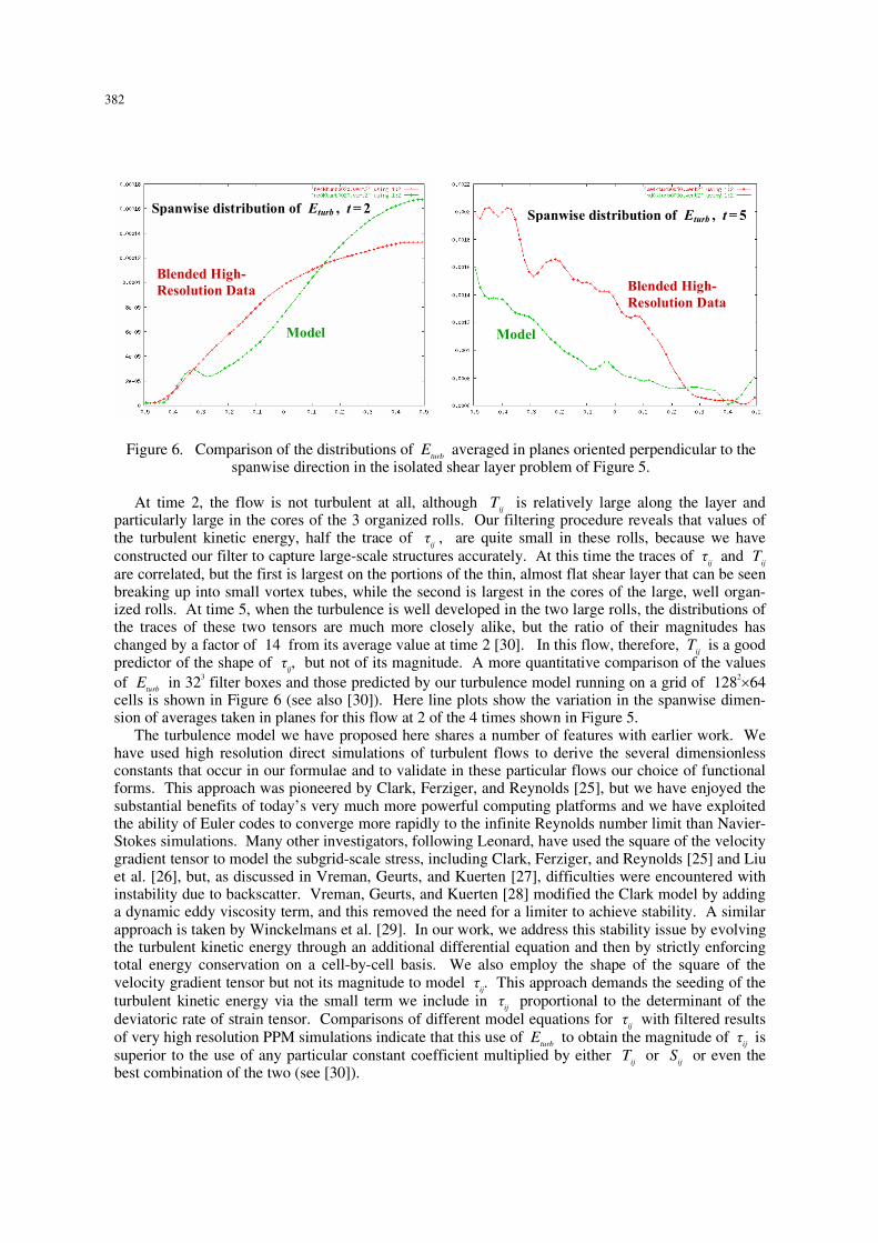Large-scale simulations of turbulent stellar convection flows and the outlook for petascale computation

Paul R Woodward David H Porter Sarah Anderson Tyler Fuchs

Laboratory for Computational Science amp Engineering University of Minnesota

and Falk Herwig

Los Alamos National Laboratory

paullcseumnedu

Abstract The late stages of stellar evolution have great importance for the synthesis and dispersal of the elements heavier than helium We focus on the helium shell flash in low mass stars where incorporation of hydrogen into the convection zone above the helium burning shell can result in production of carbon-13 with tremendous release of energy The need for detailed 3-D simulations in understanding this process is explained To make simulations of the entire helium flash event practical models of turbulent multimaterial mixing and nuclear burning must be constructed and validated As an example of the modeling and validation process our recent work on modeling subgrid-scale turbulence in 3-D compressible gas dynamics simula-tions is described and a new turbulence model presented along with supporting results Finally the potential impact of petascale computing hardware on this problem is explored

1 Introduction Only a few hundred million years after the Big Bang the earliest stars were formed from gas containing hydrogen helium and only trace concentrations of a few other light elements The heavier elements that make up planets like the earth and on which life is based were generated in stars In order to account for the abundances of these elements we need to understand the processes by which these elements are produced in nuclear reactions in early generations of stars and also how they are then expelled into the interstellar medium Stellar explosions form only a part of this story Much of the heavy element abundance is created in stars that expel their outer envelopes to form planetary nebulae Especially for the earliest generation of such stars both the production of the heavy nuclei and their transport to the circumstellar regions are sensitive to 3-D effects that have not been accurately understood Two cases of quiescent burning are distinguished by the stellas mass massive stars continue burning progressively higher-mass elements in shells until they form an iron core and collapse stars below ~10 Msun will go through H- and He-burning phases and up to C-burning for the most massive cases before they form an electron-degenerate core This core is the pre-formed white dwarf which will be the ultimate endpoint of evolution for low-mass stars Before that final stage is reached burning continues for a long time in shells surrounding the degenerate core At this time the unburned envelope is inflated to giant dimensions filling several hundred solar radii with vigorous turbulent convection These asymptotic giant branch (AGB) stars are the precursors of planetary nebulae and the subject of our interest here

Institute of Physics Publishing Journal of Physics Conference Series 46 (2006) 370ndash384doi1010881742-6596461052 SciDAC 2006

370copy 2006 IOP Publishing Ltd









371








372


373









374

2 21 12 2

( ) ( )

( )



E DEu E E ut Dt







x u

y and









375










Like the heat Eturb













376




ij in





ij is very



ij contains a





k k

uuT Lx x

4fL x and 45






377










ij in terms of T



i

i

ut x

ij i j D iji

j

p q u uut x

j

j

u E p qEt x

25 3 33 2


i i j f


3 11 2 2 j jpE q u u

1 12 3

jiij D ij ij kkij

j i

uuS S S Sx x

2 1 43


k k

uuT L T T T L xx x



D f Dijkk D Dlm lm

T Sq L ST S S




378





d

t = 186

a b

c

PPM 256

PPM2048

PPMturb 256

t = 20 t = 186

PPMturb 128

PPMturb 256

PPM 2048

t = 186

PPM 256 PPM 2048 PPM 2048

PPMturb256

379






380




381





ij





ij or S

ij or even the



Model


Model



382









383















384









371








372


373









374

2 21 12 2

( ) ( )

( )



E DEu E E ut Dt







x u

y and









375










Like the heat Eturb













376




ij in





ij is very



ij contains a





k k

uuT Lx x

4fL x and 45






377










ij in terms of T



i

i

ut x

ij i j D iji

j

p q u uut x

j

j

u E p qEt x

25 3 33 2


i i j f


3 11 2 2 j jpE q u u

1 12 3

jiij D ij ij kkij

j i

uuS S S Sx x

2 1 43


k k

uuT L T T T L xx x



D f Dijkk D Dlm lm

T Sq L ST S S




378





d

t = 186

a b

c

PPM 256

PPM2048

PPMturb 256

t = 20 t = 186

PPMturb 128

PPMturb 256

PPM 2048

t = 186

PPM 256 PPM 2048 PPM 2048

PPMturb256

379






380




381





ij





ij or S

ij or even the



Model


Model



382









383















384








372


373









374

2 21 12 2

( ) ( )

( )



E DEu E E ut Dt







x u

y and









375










Like the heat Eturb













376




ij in





ij is very



ij contains a





k k

uuT Lx x

4fL x and 45






377










ij in terms of T



i

i

ut x

ij i j D iji

j

p q u uut x

j

j

u E p qEt x

25 3 33 2


i i j f


3 11 2 2 j jpE q u u

1 12 3

jiij D ij ij kkij

j i

uuS S S Sx x

2 1 43


k k

uuT L T T T L xx x



D f Dijkk D Dlm lm

T Sq L ST S S




378





d

t = 186

a b

c

PPM 256

PPM2048

PPMturb 256

t = 20 t = 186

PPMturb 128

PPMturb 256

PPM 2048

t = 186

PPM 256 PPM 2048 PPM 2048

PPMturb256

379






380




381





ij





ij or S

ij or even the



Model


Model



382









383















384


373









374

2 21 12 2

( ) ( )

( )



E DEu E E ut Dt







x u

y and









375










Like the heat Eturb













376




ij in





ij is very



ij contains a





k k

uuT Lx x

4fL x and 45






377










ij in terms of T



i

i

ut x

ij i j D iji

j

p q u uut x

j

j

u E p qEt x

25 3 33 2


i i j f


3 11 2 2 j jpE q u u

1 12 3

jiij D ij ij kkij

j i

uuS S S Sx x

2 1 43


k k

uuT L T T T L xx x



D f Dijkk D Dlm lm

T Sq L ST S S




378





d

t = 186

a b

c

PPM 256

PPM2048

PPMturb 256

t = 20 t = 186

PPMturb 128

PPMturb 256

PPM 2048

t = 186

PPM 256 PPM 2048 PPM 2048

PPMturb256

379






380




381





ij





ij or S

ij or even the



Model


Model



382









383















384









374

2 21 12 2

( ) ( )

( )



E DEu E E ut Dt







x u

y and









375










Like the heat Eturb













376




ij in





ij is very



ij contains a





k k

uuT Lx x

4fL x and 45






377










ij in terms of T



i

i

ut x

ij i j D iji

j

p q u uut x

j

j

u E p qEt x

25 3 33 2


i i j f


3 11 2 2 j jpE q u u

1 12 3

jiij D ij ij kkij

j i

uuS S S Sx x

2 1 43


k k

uuT L T T T L xx x



D f Dijkk D Dlm lm

T Sq L ST S S




378





d

t = 186

a b

c

PPM 256

PPM2048

PPMturb 256

t = 20 t = 186

PPMturb 128

PPMturb 256

PPM 2048

t = 186

PPM 256 PPM 2048 PPM 2048

PPMturb256

379






380




381





ij





ij or S

ij or even the



Model


Model



382









383















384

2 21 12 2

( ) ( )

( )



E DEu E E ut Dt







x u

y and









375










Like the heat Eturb













376




ij in





ij is very



ij contains a





k k

uuT Lx x

4fL x and 45






377










ij in terms of T



i

i

ut x

ij i j D iji

j

p q u uut x

j

j

u E p qEt x

25 3 33 2


i i j f


3 11 2 2 j jpE q u u

1 12 3

jiij D ij ij kkij

j i

uuS S S Sx x

2 1 43


k k

uuT L T T T L xx x



D f Dijkk D Dlm lm

T Sq L ST S S




378





d

t = 186

a b

c

PPM 256

PPM2048

PPMturb 256

t = 20 t = 186

PPMturb 128

PPMturb 256

PPM 2048

t = 186

PPM 256 PPM 2048 PPM 2048

PPMturb256

379






380




381





ij





ij or S

ij or even the



Model


Model



382









383















384










Like the heat Eturb













376




ij in





ij is very



ij contains a





k k

uuT Lx x

4fL x and 45






377










ij in terms of T



i

i

ut x

ij i j D iji

j

p q u uut x

j

j

u E p qEt x

25 3 33 2


i i j f


3 11 2 2 j jpE q u u

1 12 3

jiij D ij ij kkij

j i

uuS S S Sx x

2 1 43


k k

uuT L T T T L xx x



D f Dijkk D Dlm lm

T Sq L ST S S




378





d

t = 186

a b

c

PPM 256

PPM2048

PPMturb 256

t = 20 t = 186

PPMturb 128

PPMturb 256

PPM 2048

t = 186

PPM 256 PPM 2048 PPM 2048

PPMturb256

379






380




381





ij





ij or S

ij or even the



Model


Model



382









383















384




ij in





ij is very



ij contains a





k k

uuT Lx x

4fL x and 45






377










ij in terms of T



i

i

ut x

ij i j D iji

j

p q u uut x

j

j

u E p qEt x

25 3 33 2


i i j f


3 11 2 2 j jpE q u u

1 12 3

jiij D ij ij kkij

j i

uuS S S Sx x

2 1 43


k k

uuT L T T T L xx x



D f Dijkk D Dlm lm

T Sq L ST S S




378





d

t = 186

a b

c

PPM 256

PPM2048

PPMturb 256

t = 20 t = 186

PPMturb 128

PPMturb 256

PPM 2048

t = 186

PPM 256 PPM 2048 PPM 2048

PPMturb256

379






380




381





ij





ij or S

ij or even the



Model


Model



382









383















384










ij in terms of T



i

i

ut x

ij i j D iji

j

p q u uut x

j

j

u E p qEt x

25 3 33 2


i i j f


3 11 2 2 j jpE q u u

1 12 3

jiij D ij ij kkij

j i

uuS S S Sx x

2 1 43


k k

uuT L T T T L xx x



D f Dijkk D Dlm lm

T Sq L ST S S




378





d

t = 186

a b

c

PPM 256

PPM2048

PPMturb 256

t = 20 t = 186

PPMturb 128

PPMturb 256

PPM 2048

t = 186

PPM 256 PPM 2048 PPM 2048

PPMturb256

379






380




381





ij





ij or S

ij or even the



Model


Model



382









383















384





d

t = 186

a b

c

PPM 256

PPM2048

PPMturb 256

t = 20 t = 186

PPMturb 128

PPMturb 256

PPM 2048

t = 186

PPM 256 PPM 2048 PPM 2048

PPMturb256

379






380




381





ij





ij or S

ij or even the



Model


Model



382









383















384






380




381





ij





ij or S

ij or even the



Model


Model



382









383















384




381





ij





ij or S

ij or even the



Model


Model



382









383















384





ij





ij or S

ij or even the



Model


Model



382









383















384









383















384















384

large-scale simulations of turbulent stellar convection - iopscience

Documents