- 1 -

Largest claims reinsurance: the cedant's point of view

Christian Hess1

Centre de Recherche Viablité, Jeux, Contrôle

Université Paris Dauphine

Place du Maréchal de Lattre de Tassigny

75775 PARIS CEDEX 16

FRANCE

Abstract: We present results allowing one to evaluate the cost and the variancereduction of the cedant in the framework of reinsurance treaties based on orderstatistics. We compare the efficiency of such treaties with excess of loss covers.Numerical examples show that the best choice may depend on the distribution ofthe individual claim size, especially on the heaviness of the tail. It may alsodepend on the premium principles applied by both companies.

Keywords: Largest claims reinsurance, excess of loss reinsurance, optimalreinsurance, order statistics

1tel : 00 33 (0)1 44 05 46 44 fax : 00 33 (0)1 44 05 40 36

e-mail address : Christian.Hess@dauphine.fr

- 2 -

1. IntroductionA lot of papers have been devoted to the pricing of reinsurance treaties based onthe largest claims during a given time period. Especially, since the early eightiesE. Kremer have dealt with this problem in a series of papers in various situations,using several methods. More recently, Berglund [Berg] and Walhin [Wa] havealso contributed to this subject. Essentially, the goal of these authors was thepricing of LCR and/or the ECOMOR treaties. In particular, calculations orestimations of the first two moments of the reinsurer claim expenses weredeveloped.

In the present paper, our aim is to examine the impact of LCR and ECOMORreinsurance treaties from the point of view of the reinsured, i.e. the cedant. Weprovide formulas allowing one to calculate the pure premium and the standarddeviation of the reinsured. Numerical examples are also provided. They showthat Largest Claims Reinsurance and ECOMOR covers are generally not betterthan XL Reinsurance treaties when the latter have an infinite upper limit. Only insome cases LCR treaties are a little more efficient than XL ones. The heavinessof the tail of the claim size distribution is seen to play an important part. Twotypes of premium principles are considered in this context, especially theexpectation principle and the standard deviation principle. On the other hand, thenumber of largest claims ceded to the reinsurer is also relevant.

In Section 2, we present the needed definitions and preliminaries. In Section 3 weestablish general formulas for the first two moments of the cedant's share forLCR and ECOMOR treaties. In Section 4, we compare LCR and ECOMORtreaties with an excess of loss (XL) treaty, under two possible choices of thepremium principle. Section 5 contains numerical examples. Two different claimsize distributions are considered: the translated exponential and the generalizedPareto. Our general conclusions are presented in Section 6. As to the referenceslist, in addition to papers related to our work, we have mentioned some recentbooks dealing with non life insurance or reinsurance mathematics.

2. Notations, Definitions, and PreliminariesFor a given class of risks and a given period of time, N denotes the number ofclaims and C1 , C2 , ..., Cn , ... denotes the claims sizes. The random variables Cnare assumed to be nonnegative, independent and identically distributed, and the

- 3 -

number of claims is assumed to be independent from the sequence of the claimsizes. All the random variables are assumed to be defined on a probability space(Ω, A, P). For each integer n ≥ 0, we set

pn = P(N = n).

Further, we denote by F the common distribution function of the claims sizesand we assume the existence of a density f. For every integer n ≥ 1, the sequence

C1:n ≤ C2:n ≤ ... ≤ Cn:n

stands for the sequence of the first n claims sizes in the increasing order. Inparticular

C1:n = min(C1 , C2 , ..., Cn) and Cn:n = max(C1 , C2 , ..., Cn)

are respectively the smallest and the largest claim size among C1 , C2 , ..., Cn. Wealso set Ci:n = 0 if i < 0 or i > n. For each integer k such that 1 ≤ k ≤ n, Fk:ndenotes the cumulative distribution function of Ck:n .

In the framework of the collective risk model, the total aggregate claim amount,denoted by X, has the following form

X = ∑i=1

N Ci if N > 0, 0 if N = 0.

As is well known, the first two moments of X are given by

(2.1) E(X) = E(N) E(C)

and

(2.2) Var(X) = E(N) Var(C) + Var(N) E(C)2.

In particular, when the distribution of N is Poisson with parameter λ, the aboveformulas reduce to

(2.3) E(X) = λ E(C) and Var(X) = λ E(C2).

Assume that a reinsurance treaty has been concluded between a reinsurer and areinsured (a cedant). We denote by X' (resp. X") the total aggregate claimamount paid by the reinsured (resp. the reinsurer). These random variablesobviously satisfy

X = X' + X".

- 4 -

Basically, a reinsurance treaty based on ordered claim sizes is given by asequence of functions Rn of the following type

(2.4) Rn(c1 , ..., cn) = ∑i=1

n hi(ci:n) n ≥ 1

where (hi)i≥1 denotes a given sequence of measurable functions

hi : [0, +∞ ) → [0, +∞ )

verifying0 ≤ hi(x) ≤ x x ≥ 0.

In such a case, X' and X" read as follows

(2.5) X" = RN(C1 , ..., CN) = ∑i=1

N hi(ci:N) and X' = X - X".

More precisely, X" takes on the value Rn(c1 , ..., cn) if N = n and Ci = ci for i =1, ..., n. Let us mention the following three examples, where p denotes a positiveinteger. For convenience, it is assumed that p ≤ N.

(i) The largest claims reinsurance treaty of order p, denoted by LCR(p), is definedby

X" = ∑j=1

p CN-j+1:N

Here, formula (2.4) holds withhi(x) = x if i = N-p+1, ..., N

hi(x) = 0 if i ≤ N-p

so that the reinsurer will pay the p largest claims that have occurred during agiven period of time.

(ii) The ECOMOR(p) treaty is defined by

X" = ∑j=1

p

 (CN-j+1:N  -  CN-p+1:N) = ∑j=1

p-1 CN-j+1:N  -  (p-1) CN-p+1:N

for p ≥ 2. For p = 1, we have X" = 0. In this case, formula (2.5) is valid withhi(x) = x if i = N-p+2, ..., N

- 5 -

hi(x) = (1-p) x if i = N-p+1

hi(x) = 0 if i ≤ N-p

Clearly, the p-th largest claim size plays the role of a random priority (ordeductible).

(iii) The Drop Down Excess of Loss treaty is a variant of an excess of loss (XL)treaty, where the layer may vary in function of the order of the claim, after theclaims have been ordered by increasing order. The reinsurer’s share has thefollowing form

X" = ∑i=1

N  hi(CN-i+1:N) .

For example, assume that two different excess of loss covers are involved andthat some integer p is given (1 ≤ p ≤ N). Then, formula (2.5) still holds with

hi(x) = min(t1 - s1 , max(0, x - s1)) if i = 1, ..., p-1

andhi(x) = min(t2 - s2 , max(0, x - s2)) if i = p, ..., N

where s1 (resp. s2) and t1 (resp. t2) denote the priority and the upper limit of thefirst (resp. second) XL treaty.

3. The first two moments of the reinsured share in the LCRand ECOMOR treaties

Since the total claims amount X satisfies X = X' + X" where X' (resp. X") is thereinsured (resp. reinsurer) share, we immediatly get

(3.1) E(X) = E(X') + E(X")

which allows us to deduce the expectation of the reinsured share once theexpectation of the reinsurer share is known. In the LCR(p) treaty one has

(3.2) E(X") = ∑j=1

p  E(CN-j+1:N)

and in the ECOMOR(p) treaty

(3.3) E(X") = ∑j=1

p  E(CN-j+1:N)  -  p E(CN-p+1:N) .

- 6 -

As to the variance of X', we have in both cases

(3.4) Var(X') = Var(X - X") = Var(X) + Var(X") - 2 cov(X, X")

where

(3.5) cov(X, X") = E(X X") - E(X) E(X").

Formulas for the expectation E(X") and variance Var(X") have been proposed inseveral works, especially in that of Berglund [Ber]. Thus, in view of (3.4) and(3.5) it only remains to calculate E(X X").

Berglund's formulas are recalled hereafter, because they are used in ournumerical examples in Section 5 and because the formula for E(X X") is more orless of the same type. The k-th moment of Ci:N is given by

E((Ci:N)k) = 1

(i-1)! ⌡⌠

0

1 F-1(u)k (1-u)i-1 ψ(i)(u) du

where 1 ≤ i ≤ n and k ≥ 1. As to the expectation of the cross product of the i-thand the j-th ordered claim sizes, satisfying 1 ≤ i < j ≤ n we haveE(Ci:N Cj:N) =

1(i-1)! (j-i-1)! ⌡

⌠

0

1 F-1(v) (1-v)j-1 ψ(j)(v) ⌡⌠

0

1 F-1(1-u(1-v)) ui-1 (1-u)j-i-1 du dv .

Before stating the first result of this section, it is useful to define the expressiondenoted by EN(C1 CN-j+1) for each j = 1, ..., p. It is the random variable takingon the value E(C1 Cn-j+1) with probability pn = P(N = n).

Theorem 3.1

(a) In the LCR(p) treaty the expectation of X X" is given by

E(X X") = ∑j=1

p  E(N EN(CN-j+1:N C1)) .

(b) In the ECOMOR(p) treaty, we have

E(X X") = ∑j=1 

p-1 E(N EN(C1 CN-j+1:N) ) -  (p-1) E(N EN(C1 CN-p+1:N)) .

Proof. In the LCR(p) treaty we have

- 7 -

(3.6) E(X X") = E{( ∑i=1

N Ci ) (∑

j=1

p  CN-j+1:N)} = ∑

j=1

p  E(CN-j+1:N ∑

i=1

N Ci ).

For each integer j = 1, ..., p and each n ≥ 1, the hypotheses of the collective riskmodel allow us to write

E(CN-j+1:N ∑i=1

N Ci / N = n) = E(Cn-j+1:n ∑

i=1

n Ci ) = ∑

i=1

n  E(Cn-j+1:n Ci).

The important point is that, due to the exchangeability of the sequence (Ci)i≥1 wehave

E(CN-j+1:N ∑i=1

N Ci / N = n) = n E(Cn-j+1:n C1)

which entails

E(CN-j+1:N ∑i=1

N Ci / N) = N EN(CN-j+1:N C1)

where, for each j = 1, ..., p, EN(C1 CN-j+1) is defined as above. It follows

E(CN-j+1:N ∑i=1

N Ci ) = E{E(CN-j+1:N ∑

i=1

N Ci / N)}

= E(N EN(CN-j+1:N C1))which in view of (3.6) yields the desired result. The formula for the ECOMOR(p)treaty is derived similarly. Q.E.D.

Our task is now to calculate the expectations involved in formulas (a) and (b) inTheorem 3.1. Observe first that for each j = 1, ..., p

(3.7) E(N EN(CN-j+1:N C1)) = ∑n≥j n pn E(C1 Cn-j+1:n) .

In order to calculateIk:n ;= E(C1 Cn-j+1:n),

we need to know the distribution of the pair (C1 , Ck:n), where k = n-j+1 rangesfrom 1 to n. At this point, it is important to observe that the distribution µk:n ofthe pair (C1 , Ck:n) is not absolutely continuous with respect to the Lebesguemeasure λ2 on the measurable space (R2, B(R2)), because the event {C1 = Ck:n}

- 8 -

has a non zero probability (namely 1/n). The distribution µk:n has the followingform(3.8) µk:n = 1Δ(x, y) a(x, y) λ2 + 1Δ'(x, y) b(x, y) λ2 + 1D(x) c(x) λD

where λ2 denotes the Lebesgue measure on (R2, B(R2)) and λD the Lebesguemeasure on the line D = {(x, y) in R2 : x = y}. The subsets Δ and Δ ' are definedby

Δ = {(x, y) in R2 : x < y} and Δ' = {(x, y) in R2 : x > y}.

On Δ, namely when x < y, standard differential and combinatorial arguments (seee.g. [DN] p. 11) allow us to derive the formulas

a(x, y) = (n-1)!

(k-2)! (n-k)! f(x) f(y) F(y)k-2 (1-F(y))n-k

valid for k = 2, 3, ..., n. On Δ', namely when x > y, we get similarly

b(x, y) = (n-1)!

(k-1)! (n-k-1)! f(x) f(y) F(y)k-1 (1-F(y))n-k-1

valid for k = 1, 2, ..., n-1. On the line D, function c(.) given by

c(x) = (n-1)!

(k-1)! (n-k)! f(x) F(x)k-1 (1-F(x))n-k.

When k = 1, one has a(x, y) = 0 because the event {C1 < C1:n} is impossible.Similarly, when k = n one has b(x, y) = 0, because the event {C1 > Ck:n} isimpossible. Using the above formulas, we get

Ik:n = ⌡⌠ ⌡⌠

  Δ xy a(x, y) dx dy + ⌡⌠ ⌡⌠

  Δ'

xy b(x, y) dx dy + ⌡⌠  D x2 c(x) dx

It is also convenient to introduce the function H by

(3.9) H(z) = ⌡⌠0

z t f(t) dt z ≥ 0

which satisfies H(+∞) = E(C) = m. From the above formulas, we infer

Ik:n = (n-1)!

(k-2)! (n-k)! ⌡⌠

0

+ ∞  y f(y) F(y)k-2 (1-F(y))n-k H(y) dy

+ (n-1)!

(k-1)! (n-k-1)! ⌡⌠

0

+ ∞  y f(y) F(y)k-1 (1-F(y))n-k-1 (m - H(y)) dy

- 9 -

+ (n-1)!

(k-1)! (n-k)! ⌡⌠

0

+ ∞  x2 f(x) F(x)k-1 (1-F(x))n-k dy .

After substituting v = F(y) in the first two integrals and u = F(x) in the third one,we get

Ik:n = (n-1)!

(k-2)! (n-k)! ⌡⌠

0

1  F-1(v) vk-2 (1-v)n-k H(F-1(v)) dv

+ (n-1)!

(k-1)! (n-k-1)! ⌡⌠

0

1  F-1(v) vk-1 (1-v)n-k-1 (m - H(F-1(v))) dv

+ (n-1)!

(k-1)! (n-k)! ⌡⌠

0

1  F-1(u)2 uk-1 (1-u)n-k du .

Equivalently, since k = n-j+1 we haveIn-j+1:n = T1(n, j) + T2(n, j) + T3(n, j)

where

T1(n, j) = (n-1)!

(n-j-1)! (j-1)! ⌡⌠

0

1  F-1(v) vn-j-1 (1-v)j-1 H(F-1(v)) dv

T2(n, j) = (n-1)!

(n-j)! (j-2)! ⌡⌠

0

1  F-1(v) vn-j (1-v)j-2 (m - H(F-1(v))) dv

T3(n, j) = (n-1)!

(n-j)! (j-1)! ⌡⌠

0

1  F-1(u)2 un-j (1-u)j-1 du .

According to a previous observation, the first term is absent if j = n and thesecond one is absent if j = 1. Now, we turn to the computation of

(3.10) E(N E(C1 CN-j+1:N)) = ∑n≥j+1

  pn T1(n, j) + ∑n≥j  pn T2(n, j)

+ ∑n≥j  pn T3(n, j) .

As to the first summation in (3.10), we get

∑n≥j+1

  pn T1(n, j)

- 10 -

= 1

(j-1)! ⌡⌠

0

1  F-1(v) (1-v)j-1 H(F-1(v)) ( ∑

n≥j+1  

n!(n-j-1)! vn-j-1) dv

= 1

(j-1)! ⌡⌠

0

1  F-1(v) (1-v)j-1 H(F-1(v)) ψN(j+1)(v) dv

where ψN(j+1) denotes the (j+1)th derivative of ψN , the probability generatingfunction of N. Recall that

ψN(t) = E(tN) 0 ≤ t ≤ 1.

As to the second and third summation in (3.10), we get similarly

∑n≥j  pn T2(n, j) =

1(j-2)! ⌡

⌠

0

1  F-1(v) (1-v)j-2 (m - H(F-1(v))) ψN(j)(v) dv

∑n≥j  pn T3(n, j) =

1(j-1)! ⌡

⌠

0

1  F-1(u)2 (1-u)j-1 H(F-1(u)) ψN(j)(u) dv.

Consequently, we have proven the following result.

Theorem 3.2

For each j = 1, ..., p one has

E(N EN(C1 CN-j+1:N)) = 1

(j-1)! ⌡⌠

0

1  F-1(v) (1-v)j-1 H(F-1(v)) ψN(j+1)(v) dv

+ 1

(j-2)! ⌡⌠

0

1  F-1(v) (1-v)j-2 (m - H(F-1(v))) ψN(j)(v) dv

+ 1

(j-1)! ⌡⌠

0

1  F-1(u)2 (1-u)j-1 ψN(j)(u) du.

Theorem 3.2 allows us to derive formulas for E(X X") in the LCR andECOMOR treaties. In view of (3.4), we also need to determine Var(X"). In theLCR(p) treaty we have

Var(X") = ∑j=1

p Var(CN-j+1:N) + 2∑

j=2

p 

∑

i=1j-1 cov(CN-i+1:N , CN-j+1:N).

In the ECOMOR(p) treaty, the following formula holds

- 11 -

Var(X") = ∑j=1

p-1 Var(CN-j+1:N) + (p-1)2 Var(CN-p+1:N)

+ 2∑j=2

p-1  ∑

i=1

j-1 cov(CN-i+1:N , CN-j+1:N)

- 2(p-1) ∑i=2

p-1  cov(CN-i+1:N , CN-p+1:N).

General formulas allowing for evaluatingE(CN-j+1:N) Var(CN-j+1:N) and cov(CN-i+1:N , CN-j+1:N)

have been recalled in the beginning of this section. Using these formulas and theabove relationships, and returning to (3.4), it is now possible to derive formulasfor Var(X') in the LCR and ECOMOR treaties. These formulas will be used inSection 5, as well as formulas of Theorems 3.1 and 3.2.

4. Comparison of LCR and ECOMOR reinsurance withExcess-of-Loss Reinsurance

It is interesting to compare the efficiency of LCR and ECOMOR treaties with theexcess of loss (XL) treaty that is frequently used in the reinsurance world. Forthis purpose, we consider an XL treaty whose priority is denoted by s and whoseupper limit is +∞.

The comparison will be done along the following lines. Generally speakinginsurance and reinsurance premiums include a safety loading that is added to thepure premium in order to increase insurers' solvency. More precisely, if X standsfor the aggregate claim amount relative to a group of risks during a given timeperiod, the loaded premium Π(X) will have the following form

(4.1) Π(X) = E(X) + SL(X)

where SL(X) denotes the safety loading. This loading is chosen in reference tosome premium principle. For example, according to the expectation principle, thesafety loading will be

SL(X) = α E(X)

where α is a suitable positive coefficient. If the insurer has chosen the standarddeviation principle, the safety loading will read as

- 12 -

SL(X) = α σ(X).

This is also valid in the framework of a reinsurance treaty. In a similar way, thereinsurance premium, denoted by Πr(X"), has the following form

(4.2) Πr(X") = E(X") + SLr(X")

where X" denotes the reinsurer share, as above, and SLr(X") denotes thecorresponding safety loading. If the reinsurer applies the expectation principle(resp. standard deviation principle), the safety loading will be given by SLr(X") =β E(X") (resp. SLr(X") = β σ(X")), where β is a positive coefficient (possiblydifferent from α).

Further, we consider the underwriting profit (profit for short) of the insurer, i.e.not including financial benefits. In the absence of reinsurance, it is obviously equalto

Π(X) - X.

After a reinsurance arrangement has taken place, the claim expenses are dividedaccording to the usual formula, i.e.

X = X' + X"

where X' (resp. X") stands for the reinsured (resp. reinsurer) share. Then, theinsurer profit, denoted by Z, becomes

Z = Π(X) - X' - Πr(X").

In view of (4.1) and (4.2), it is readily seen that its first two moments are givenby(4.3) E(Z) = SL(X) - SLr(X") and σ(Z) = σ(X').

In particular, if both the cedant and the reinsurer use the expectation principle(case I), we get

E(Z) = α E(X) - β E(X").

If the standard deviation principle is used (case II), we get

E(Z) = α σ(X) - β σ(X").

The comparison between XL reinsurance and LCR or ECOMOR reinsurancewill be done as follows. For example, consider the LCR(p) treaty and the XLtreaty with priority s, denoted by XL(s). If the XL treaty is in force, we canexpress X as

- 13 -

X = Y'(s) + Y"(s)

where Y'(s) (resp. Y"(s)) denotes the reinsured (resp. the reinsurer) share in theXL(s) treaty. Recall that

Y'(s) = ∑i=1

N  Ci'(s) and Y"(s) = ∑

i=1

N  Ci"(s)

where Ci'(s) and Ci"(s) are given by

Ci'(s) = min(Ci , s) and Ci"(s) = max(0, Ci - s)

for all i = 1, ..., N. As for the LCR(p) treaty, we can write

X = X'(p) + X"(p)

where the variable p refers to the LCR(p) treaty, i.e. to the number of claims paidby the reinsurer.

We begin by computing the priority, say s#, such that the expectation of theinsured profit takes on the same value after the applicaton of both treaties.Namely, s# satisfies the equation(4.4) SL(X) - SLr(X"(p)) = SL(X) - SLr(Y"(s#))

or equivalently(4.5) SLr(X"(p)) = SLr(Y"(s#)).

Then, we compare the standard deviations of the reinsured share in the LCR(p)treaty and in the XL(s#) treaty, namely σ(X'(p)) and σ(Y'(s)).

In case I, equation (4.5) becomes E(X"(p)) = E(Y"(s#)). and in case II, σ(X"(p)) =σ(Y"(s#)). Further, if the number of claims is Poisson distributed with parameterλ, formulas (2.3), applied to Y"(s#), yields

(4.6) E(X"(p)) = λ E(C"(s#)) (case I)

and

(4.7) σ(X"(p)) =  λ E(C"(s#)2)  (case II).

Of course, the value of the root s# is not the same in (4.6) and in (4.7).

Remark 4.1

When the safety loading is based on the expectation principle, pure premiums forLCR (or ECOMOR) and XL treaties are equal, as shown by equation (4.6). This

- 14 -

is no longer true when the safety loading is based on the standard deviationprinciple. In this case, the equality holds between the standard deviation of thereinsurer share relative to LCR or ECOMOR and XL treaties. This is expressedby equation (4.7).

Remark 4.2

The following ratio, denoted by T is often used as a simple measure of solvency

T = R + E(Z)σ(Z)

where R stands for the amount of the risk reserve and Z for the cedant's profitas defined above. The ratio T, referred to as the solvency coefficient, is closelyconnected to the ruin probability. Higher values of T correspond lower values ofruin probability, thus to better solvency level. According to equation (4.3) wehave

(4.8) T = R + SL(X) - SLr(X")

σ(X') .

This is valid for any reinsurance treaty. In particular, when the safety loading isbased on the expectation principle, (4.8) becomes

(4.9) T = R + α E(X) - β E(X")

σ(X')

and when it is based on the standard deviation principle

(4.10) T = R + α σ(X) - β σ(X")

σ(X') .

In (4.9) and (4.10), the loading coefficients α and β are then involved, as onecould expect.

On the other hand, consider for example the LCR(p) and the XL(s) treaties.Then, the solvency coefficient T is given by

(4.11) TLCR(p) = R + SL(X) - SLr(X"(p))

σ(X'(p))

for the LCR(p) treaty and by

(4.12) TXL(s) = R + SL(X) - SLr(Y"(s))

σ(Y'(s))

for the XL(s) treaty. Observe that, from equation (4.4), the numerators in (4.11)and (4.12) are equal, which implies

- 15 -

TLCR(p)TXL(s) =

σ(Y'(s))σ(X'(p)) .

In particular, the inequality σ(X'(p)) ≤ σ(Y'(s)) is equivalent to TLCR(p) ≥ TXL(s).

Remark 4.3

In order to compare XL and LCR (or ECOMOR) treaties we have consideredthe cedant's underwriting profit and we have chosen the priority s of the XLtreaty so that the profit is unchanged. However, the comparison could have beenbased on other criteria. Let us cite for example the loaded premium ratio

Π(X) - Πr(X")Π(X) = 1 -

Πr(X")Π(X)

which represents the fraction of the premium retained by the cedant.

5. Numerical ExamplesNumerical examples are given below for the LCR(p) and the ECOMOR(p)treaties, when the number of claims is Poisson distributed with parameter λ = 40and the individual claim distribution is either translated exponential or generalizedPareto. These distributions are strongly different in that the translated exponentialhas a light tail, whereas the generalized Pareto has an heavy tail. Further, in viewof the comparison with the XL treaty, we have considered two kinds of safetyloading, namely the safety loading based on the expectation principle (case I) andthe safety loading based on the standard deviation principle (case II).

When the claim size C is translated exponential distributed, its cumulativedistribution function F is given by

F(x) = 1 - exp(α (x - x0)) if x ≥ x0 , 0 if x < x0

where the parameters x0 and α are positive. Here we have chosen

x0 = 500 and α = 0,01.

In this case, it follows from (2.1) and (2.2) that E(X) = 24 000 and σ(X) =3847,08. As to the generalized Pareto, the cumulative distribution function isgiven by

F(x) = 1 - ( x0 + bx + b )α if x ≥ x0 , 0 otherwise,

- 16 -

where the parameters must satisfy x0 > 0, α > 0 and b > -x0 . Here we havechosen x0 = 100, b = 500 and α = 2.5, which entails E(X) = 20 000 and σ(X) =6480,74.

Eight tables are presented hereafter in order to illustrate the previous discussion.In Tables 1, 1 bis, 3 and 3 bis, the claim size distribution is the translatedexponential, in the other ones it is the generalized Pareto. In Tables 1 to 2 bis it isassumed that both the cedant and the reinsurer apply the pure premiumprinciple, whereas in Tables 3 to 4 bis, the cedant and the reinsurer are assumedto use the standard deviation principle. Further, Tables 1, 2, 3 and 4 concernLCR treaties, whereas Tables 1 bis, 2 bis, 3 bis and 4 bis concern ECOMORtreaties.

In each table, the first column shows the values of p, the number of the largestclaims involved in LCR or ECOMOR treaty, the second one shows thecorresponding values of the pure premium retained by the cedant. The thirdcolumn displays the standard deviation of the cedant's share, according to thereinsurance arrangement (LCR or ECOMOR). The fourth column displays thepriority s# of the XL treaty that produces the same profit for the cedant (takinginto account the principle that has been chosen for calculating the safety loading).The fifth column contains the values of the pure premium ratio (PPR), namely

E(X')E(X) .

The sixth column shows the standard deviation ratio relative to the LCR orECOMOR treaty, namely

σ(X'LCR)σ(X) or

σ(X'ECO)σ(X) .

In the tables, these ratios are also denoted by SDR-LCR and SDR-ECO. The lastcolumn shows the standard deviation ratio relative to the XL(s#) treaty. It isdenoted by SDR-XL and defined by

σ(X'XL)σ(X) .

Each table is followed by a figure that displays the data of the last two columnand allows us to compare visually the efficiency of LCR or ECOMOR treatywith the XL one.

- 17 -

TABLE 1. LCR vs XL for the translated exponentialsafety loading based on the expectation principle

p E(X'(p)) σ(X'(p)) priority PPR SDR-LCR SDR-XL1 23 073 3 822 646,25 0,961 0,994 0,9522 22 247 3 801 582,48 0,927 0,988 0,9163 21 470 3 780 545,81 0,895 0,983 0,8834 20 727 3 760 520,06 0,864 0,977 0,8525 20 009 3 741 500,22 0,834 0,972 0,8226 19 310 3 723 482,76 0,805 0,968 0,7947 18 629 3 704 465,72 0,776 0,963 0,7668 17 961 3 686 449,04 0,748 0,958 0,7389 17 307 3 668 432,66 0,721 0,954 0,71110 16 663 3 651 416,57 0,694 0,949 0,685

FIGURE 1. LCR vs XL for translated exponential -safety loading based on the expectation

0,000

0,200

0,400

0,600

0,800

1,000

1,200

1 2 3 4 5 6 7 8 9 10

p

stan

dard

de

viat

ion

rati

os

SDR-LCR SDR-XL

- 18 -

TABLE 1 bis. ECOMOR vs XL for the translated exponentialsafety loading based on the expectation principle

p E(X'(p)) σ(X'(p)) priority PPR SDR-ECO SDR-XL1 0 0 0 0 0 02 23 900 3 846 868,89 0,996 1,000 0,9933 23 800 3 844 799,57 0,992 0,999 0,9884 23 700 3 843 759,03 0,988 0,999 0,9825 23 600 3 842 730,26 0,983 0,999 0,9776 23 500 3 841 707,94 0,979 0,998 0,9727 23 400 3 839 689,71 0,975 0,998 0,9678 23 300 3 838 674,30 0,971 0,998 0,9639 23 200 3 837 660,94 0,967 0,997 0,95810 23 100 3 835 649,17 0,962 0,997 0,953

FIGURE 1 bis. ECOMOR vs LCR for translated exponential - safety loading based on the expectation

0,9300,9400,9500,9600,9700,9800,9901,0001,010

1 2 3 4 5 6 7 8 9

p

stan

dard

de

viat

ion

rati

os

SDR-ECO SDR-XL

- 19 -

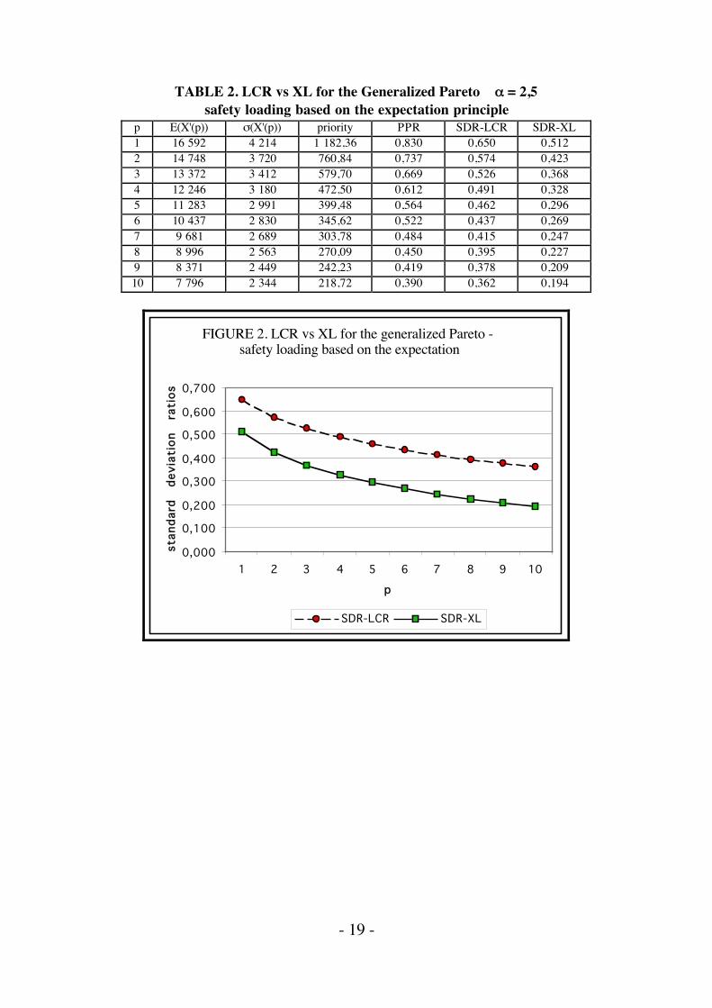
TABLE 2. LCR vs XL for the Generalized Pareto α = 2,5safety loading based on the expectation principle

p E(X'(p)) σ(X'(p)) priority PPR SDR-LCR SDR-XL1 16 592 4 214 1 182,36 0,830 0,650 0,5122 14 748 3 720 760,84 0,737 0,574 0,4233 13 372 3 412 579,70 0,669 0,526 0,3684 12 246 3 180 472,50 0,612 0,491 0,3285 11 283 2 991 399,48 0,564 0,462 0,2966 10 437 2 830 345,62 0,522 0,437 0,2697 9 681 2 689 303,78 0,484 0,415 0,2478 8 996 2 563 270,09 0,450 0,395 0,2279 8 371 2 449 242,23 0,419 0,378 0,20910 7 796 2 344 218,72 0,390 0,362 0,194

FIGURE 2. LCR vs XL for the generalized Pareto -safety loading based on the expectation

0,000

0,100

0,200

0,300

0,400

0,500

0,600

0,700

1 2 3 4 5 6 7 8 9 10

p

stan

dard

de

viat

ion

rati

os

SDR-LCR SDR-XL

- 20 -

TABLE 2 bis. ECOMOR vs XL for the Generalized Pareto α = 2,5safety loading based on the expectation principle

p E(X'(p)) σ(X'(p)) priority PPR SDR-ECO SDR-XL1 0 0 0 0 0 02 18 437 4 829 2 328,62 0,922 0,745 0,6373 17 499 4 459 1 567,73 0,875 0,688 0,5664 16 749 4 230 1 235,93 0,837 0,653 0,5215 16 099 4 058 1 037,25 0,805 0,626 0,4866 15 513 3 919 900,49 0,776 0,605 0,4577 14 975 3 800 798,57 0,749 0,586 0,4338 14 472 3 695 718,63 0,724 0,570 0,4119 13 999 3 602 653,62 0,700 0,556 0,39210 13 548 3 517 599,32 0,677 0,543 0,375

FIGURE 2 bis. ECOMOR vs XL for generalized Pareto -

safety loading based on the expectation

0,0000,1000,2000,3000,4000,5000,6000,7000,800

1 2 3 4 5 6 7 8 9

p

stan

dard

de

viat

ion

rati

os

SDR-ECO SDR-XL

- 21 -

TABLE 3. LCR vs XL for the translated exponentialsafety loading based on the standard deviation principle

p E(X'(p)) σ(X'(p)) priority PPR SDR-LCR SDR-XL1 23 073 3 822 888,43 0,961 0,994 0,9942 22 247 3 801 810,67 0,927 0,988 0,9893 21 470 3 780 766,74 0,895 0,983 0,9844 20 727 3 760 736,16 0,864 0,977 0,9785 20 009 3 741 712,73 0,834 0,972 0,9736 19 310 3 723 693,73 0,805 0,968 0,9697 18 629 3 704 677,76 0,776 0,963 0,9648 17 961 3 686 663,98 0,748 0,958 0,9599 17 307 3 668 651,88 0,721 0,954 0,95410 16 663 3 651 641,08 0,694 0,949 0,950

FIGURE 3. LCR vs XL for the transated exponential -safety loading on the standard deviation

0,920

0,930

0,940

0,950

0,960

0,970

0,980

0,990

1,000

1 2 3 4 5 6 7 8 9 10

p

stan

dard

devia

tio

n

rati

os

SDR-LCR SDR-XL

- 22 -

TABLE 3 bis. ECOMOR vs XL for the translated exponentialsafety loading based on the standard deviation principle

p E(X'(p)) σ(X'(p)) priority PPR SDR-ECO SDR-XL1 0 0 0 0 0 02 23 900 3 846 938,20 0,996 1,000 0,9963 23 800 3 844 868,89 0,992 0,999 0,9934 23 700 3 843 828,34 0,988 0,999 0,9915 23 600 3 842 799,57 0,983 0,999 0,9886 23 500 3 841 777,26 0,979 0,998 0,9857 23 400 3 839 759,03 0,975 0,998 0,9828 23 300 3 838 743,61 0,971 0,998 0,9809 23 200 3 837 730,26 0,967 0,997 0,97710 23 100 3 835 718,48 0,962 0,997 0,975

FIGURE 3 bis. ECOMOR vs XL for the translated exponential - safety loading based on the standard

deviation

0,9600,9650,9700,9750,9800,9850,9900,9951,0001,005

1 2 3 4 5 6 7 8 9

p

stan

dard

devia

tio

n

rati

os

SDR-ECO SDR-XL

- 23 -

TABLE 4. LCR vs XL for the Generalized Pareto α = 2,5safety loading based on the standard deviation principle

p E(X'(p)) σ(X'(p)) priority PPR SDR-LCR SDR-XL1 16 592 4 214 2 813,31 0,830 0,650 0,6682 14 748 3 720 1 730,65 0,737 0,574 0,5853 13 372 3 412 1 323,95 0,669 0,526 0,5344 12 246 3 180 1 094,60 0,612 0,491 0,4975 11 283 2 991 941,79 0,564 0,462 0,4666 10 437 2 830 830,22 0,522 0,437 0,4417 9 681 2 689 743,94 0,484 0,415 0,4198 8 996 2 563 674,48 0,450 0,395 0,3999 8 371 2 449 616,93 0,419 0,378 0,38110 7 796 2 344 568,16 0,390 0,362 0,364

FIGURE 4. LCR vs XL for the generalized Pareto - safety loading based on the standard deviation

0,000

0,100

0,200

0,300

0,400

0,500

0,600

0,700

0,800

1 2 3 4 5 6 7 8 9 10

p

stan

dard

devia

tio

n

rati

os

SDR-LCR SDR-XL

- 24 -

TABLE 4 bis. ECOMOR vs LCR for the Generalized Pareto α = 2,5safety loading based on the standard deviation principle

p E(X'(p)) σ(X'(p)) priority PPR SDR-ECO SDR-XL1 0 0 0 0 0 02 18 437 4 829 3 757,13 0,922 0,745 0,7113 17 499 4 459 2 439,66 0,875 0,688 0,6454 16 749 4 230 1 924,70 0,837 0,653 0,6045 16 099 4 058 1 629,00 0,805 0,626 0,5746 15 513 3 919 1 429,94 0,776 0,605 0,5497 14 975 3 800 1 283,64 0,749 0,586 0,5288 14 472 3 695 1 169,97 0,724 0,570 0,5109 13 999 3 602 1 078,15 0,700 0,556 0,49410 13 548 3 517 1 001,87 0,677 0,543 0,479

FIGURE 4 bis. ECOMOR vs LCR for the generalized Pareto - safety loading based on standard deviation

0,000

0,1000,200

0,3000,400

0,500

0,6000,700

0,800

0 1 2 3 4 5 6 7 8 9 10

p

stan

dard

devia

tio

n

rati

os

SDR-ECO SDR-XL

In the above examples, it can be seen that the XL treaty is always more efficientthan the ECOMOR treaty, in that it produces a smaller standard deviation for thecedant for the same cost. In addition, the XL treaty is often more efficient thanthe LCR treaty. However, when the safety loading is based on the standarddeviation principle, the LCR treaty is a little better than the XL treaty. But it isworthwhile to note that we have assumed that the upper limit of the XL treaty isinfinite, which is not realistic. Thus, the efficiency of the XL treaty might bebetter in the presence of a finite upper limit. On the other hand, it can be seenthat the SDR-gap between the LCR (or ECOMOR) treaty and the XL treatyincreases with the number p of claims in consideration.

- 25 -

It can be also observed that in all treaties the variance reduction is higher for thegeneralized Pareto than for the translated exponential. This must be connected tothe fact that the generalized Pareto has a heavier tail than the translatedexponential.

As to the numerical computations, they have been performed using the formulaspresented in Section 3, with the Maple 9.5 software. The Monte-Carlo methodhas also been used for the translated exponential distribution. As for thegeneralized Pareto distribution with α = 2.5, the Monte Carlo method wasavailable for the expectation, but not for the standard deviation. Indeed, althoughthe theoretical variance Var(C) exists, the variance of its estimator, namely thesample variance, involves the moment of order 4 of the distribution, which isinfinite. Thus, the convergence of the sample variance in the Monte Carloalgorithm is not good.

The numerical results given by Berglund for the moments of the reinsurer's shareshow that replacing the Poisson distribution by the negative binomial distributiondoes not produce major changes. A similar behavior can be conjectured for thecedant's share.

6. ConclusionIn this work, we have derived formulas allowing one to calculate the expectationand, more importantly, the variance of the cedant's share in the framework of theLCR or ECOMOR treaty. We have also compared the efficiency of such treatieswith the XL treaty by some numerical examples, under two different hypotheseson the safety loading. In these examples, we have observed that the XL treatyalways dominates the ECOMOR treaty. For the LCR treaty the situation is morecomplex. In some cases, the LCR treaty is a little better than the XL treaty,especially when the safety loading is based on the standard deviation.

Of course, other examples could be considered in order to get more information.Especially, the case of XL treaties with finite upper limit could be of interest.

Further, a natural question arising from the present paper is that of the optimalityof a reinsurance treaty among a given class of treaties from the cedant's point ofview. In view of the above numerical examples, one could also ask the followingsimpler question: is it possible to find conditions under which a LCR treaty isbetter than an XL treaty ? A theoretical result on the comparison of LCR andECOMOR treaties is also strongly suggested by the numerical results.

- 26 -

On the other hand, we have only considered moments or order 1 and 2.However, it is known that the real aggregate claim amount distributions as wellas the claim size distribution are seldom symmetric. Thus, the introduction ofmoments of higher order, especially of order 3, could be pertinent.

Acknowledgment: The author is glad to thank Mrs. M.P. Hess, Senior Actuary,for a careful reading of the manuscript and for useful discussions.

References[BloPa] J. Blondeau and Ch. Partrat, La réassurance - Approche technique,Economica, 2003

[Ben] G. Benktander, Largest claims reinsurance (LCR). A quick method tocalculate LCR-risk rates from excess of loss risk rates, ASTIN Bulletin, 1978,Vol. 10, No. 1, pp. 54-58

[Berg] R. M. Berglund, A note on the net premium for a generalized largestclaims reinsurance cover, ASTIN Bulletin, 1998, Vol. 28, No. 1, pp. 153-162

[Ber] B. Berliner, Correlations between excess of loss reinsurance covers andreinsurance of the n largest claims, ASTIN Bulletin, 1972, Vol. 6, No. 3, pp. 260-275

[BesPa] J.-L. Besson and Ch. Partrat, Assurance non-vie - Modélisation,simulation, Economica, 2005

[CD] A. Charpentier and M. Denuit, Mathématiques de l'sssurance non-vie, tome1 : principes fondamentaux et théorie du risque, Economica, 2004

[DN] H.A. David and H.N. Nagaraja, Order Statistics, Third Edition, Wiley, 2003

[Kre1] E. Kremer, Rating of largest claims and ECOMOR reinsurance treatiesfor large portfolios, ASTIN Bulletin, 1982, Vol. 13, pp. 47-56

[Kre2] E. Kremer, An asymptotic formula for the net premium of somereinsurance treaties, Scandinavian Actuarial Journal, 1984, pp. 11-22

[Kre3] E. Kremer, Finite formulas for the general reinsurance treaty based onordered claims, Insurance: Mathematics and Economics, 1986, Vol. 4, 1985, pp.233-238

[Kre4] E. Kremer, Simple formulas for the premiums of the LCR andECOMOR treaties under exponential claim sizes, Blatter des DeutschenGesellschaft fur Versicherungsmathematik, 1986, Vol. 17, 457-469

- 27 -

[Kre5] E. Kremer, A general bound for the net premium of the largest claimsreinsurance covers, ASTIN Bulletin, 1988, Vol. 18, pp. 69-78

[Pe] P. Petauton, Théorie de l'assurance dommages, Dunod, 2000

[Wa] J.-F. Walhin, On the practical pricing of reinsurance treaties based on orderstatistics, Bulletin Français d'Actuariat, 2003, Vol. 6, No. 10, 169-184