laser paper

J. Instrum. Soc. India 33 (4) 229-233

STUDY OF LASER BASED TRANSMISSION/RECEPTION PARAMETERS UNDER

FADING MEDIUMS

Sameer Lakhra, Davinder Pal Sharma and Dr. Jasvir SinghDept. of Electronics Technology, Guru Nanak Dev University, Amritsar-143005

ABSTRACT

Laser as a communication medium can provide a good substitute for the present daycommunication systems as the problem of interference faced in case of electromagneticwaves is not there and high deal of secrecy is available. The present paper involves thestudy of wireless, open channel communication system using laser a carrier for voicesignals. Different fading materials with different transmission co-efficients and differentthickness are used as mediums for the transmission of coded laser light signals. Resultsobtained can be used for the fabrication of high speed, interference free opticalcommunication and perhaps in fabrication of optical fibers of presented materials also.

1. INTRODUCTIONUse of laser in communication systems is the future because of the advantages of the

full channel speeds, no communication licenses required at present [1], compatibility with copperor fiber interfaces and no bridge or router requirements [2]. Besides this there are no recurringline costs, portability, transparency to networks or protocols, although range is limited to afew hundred meters. Also the laser transmission is very secure because it has a narrow beam(any potential evesdropping will result in an interruption which will alert the personnel. Alsoit cannot be detected with use of spectrum analyzers and RF meters and hence can be usedfor diverse applications including financial, medical and military. Lasers can also transmit throughglass, however the physical properties of the glass have to be considered. Laser transmitterand receiver units ensure easy, straightforward systems alignment and long-term stable, service-free operation, especially in inaccessible environments, optical wireless systems offer ideal,economical alternative to expensive leased lines for buildings.

The laser can also be commissioned in satellites for communication, as laser radar requiressmall aperture as compared to microwave radar[3]. Also there is high secrecy and nointerference like in EM waves[4]. Further, potential bandwidth of radar using lasers can translateto very precision range measurement. For these reasons, they can be used as an alternative topresent modes of communication. Fig (1) below shows future information network using lasercommunication, which is both wide-band and high-speed [5].

230

2. EXPERIMENTAL SET-UPThis paper deals with study of wireless open channel communication using laser as a

carrier for speech message (modulating signal). For the purpose of transmitter circuit, acondenser mike, an IC-UA741-OP-AMP (whose gain is controlled by 1MΩ potentiometer)and a laser torch (wavelength 630nm) are used as main components[6]. The Receiver circuituses a phototransistor L14F1, a 2-stage preamplifier prior to IC-LM386 audio power amplifierand then a loudspeaker. The laser-coded signal when positioned on the phototransistor (selectedbecause it’s high absorption coefficient and excellent responsivity) [7], if followed by tunedamplifier, responds only to frequency of operation. The volume is controlled by a 10 KΩpotentiometer. To avoid a 50Hz, hum noise, phototransistor is kept away from a.c. sources.It is also shielded from direct sunlight. The outputs of transmitter and receiver are then givento dual channel digital CRO (Cathode Ray Oscilloscope) and the 2.5 – Mb (Megabyte) lineWebcam captures the pictures, which are analyzed. In CRO, 1µs is taken as the unit on timeaxis. Fig (2) shows CRO and its waveforms being captured by the Webcam basic experimentalset-up for the study purpose.

Variation is studied on following parameters :

A. Distance between Transmitter and Receiver.

B. Medium between transmitter and receiver (depending upon transmission coefficientand thickness of various media used for the 630nm laser waves used).

Fig-1 : Future information network using laser communication

Sameer Lakhra, Davinder Pal Sharma and Dr. Jasvir Singh

231

Fig-2 : Schematic diagram of study of parameters under fading medium

3. RESULTS AND DISCUSSION

1) Firstly, the transmitter and receiver waveform variation was observed on digital CROby changing the distance between the laser torch in transmitter and phototransistor in thereceiver using air as medium. Upto 4.5 feet, there is no variation observed in the outputwaveforms. But with increase in the distance there is waveform variation due to noise.

2) The medium between the transmitter and receiver is then changed to transparent plastic(2 fold), thicker version of same plastic (4 fold) and blue coloured polythene, sequentially.These have 10, 10.18 and 49 as values of absorption coefficients respectively as calculatedby their percentage transmission found using Ultra-Violet Spectrophotometer (in visible range)and by their respective thickness, which are 0.07mm, 0.15mm and 0.02mm (measured usinga screw gauge).

Absorption coefficient α is given by : α = (1/t) loge [100 / % T]

Where t = thickness

& % T = Percentage transmission (of each medium)

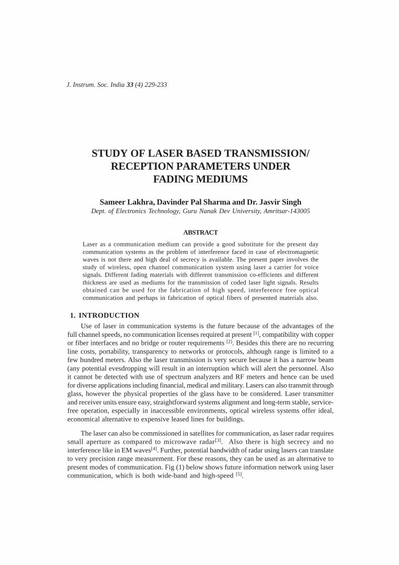
Pictures of waveforms on CRO are captured using 2.5 MB data line Webcam. Study ofwaveform results shows that attenuation increases as the distance is increased between thetransmitter and receiver (in all three media) and harmonics gets introduced. Also the pulses inthe receiver output waveform decrease in time duration. Graphs are plotted on interpretationof waveforms and the analysis is shown in Fig (3), Fig (4) and Fig (5).

The graphs show that the pulses in the receiver output waveform decrease in time duration.While the pulse decrease in case of blue polythene is very sharp, it is less sharp in case of 4fold transparent plastic and least in 2 fold transparent plastic (as distance foot between thetransmitter and the receiver is increased from 1 foot to 2 and to 3 foot). Graphs also showthat there is frequency deviation in all three cases. This shown in Table 1

Study of Laser Based Transmission/Reception Parameters under fading mediums

232

Fig-3 : Variation of pulse duration withdistance in case of blue polythene

Fig (4) Variation of pulse duration withdistance in case of 2 fold transparent plastic

Fig-5 : Variation of pulse duration with distance in case of 4 fold transparent plastic.

Table 1 : Frequency Deviation in various media:

Sl.No. Medium Frequency Deviation of (in kHz)

From 1 to 2 foot From 2 to 3 foot

1. Blue polythene 0.375 0.67

2. 4 fold transparent plastic 0.175 0.45

3. 2 fold transparent plastic 0.075 0.09

Sameer Lakhra, Davinder Pal Sharma and Dr. Jasvir Singh

233

4. CONCLUSIONThe study reveals that there is attenuation in the various media depending on the absorption

coefficient. As the observation table shows that there is high frequency deviation in case ofblue polythene, less in 4 fold transparent plastic, and least in 2 fold transparent plastic. Thisstudy is useful as an application in field of optical telecommunication and even in defenceapplications such as wireless communication.

5. REFERENCES1) John Gower, ‘Optical Communication Systems’, 2nd Edition, PHI, New Delhi (1996).

2) http://laserinfrared wireless.com/faq.htm

3) Christopher Allen ET. Al. ‘Development of a 1310nm, Coherent Laser Radar with R.F. PulseCompression’, Proceeding of IEEE IGARSS Conference (2000).

4) A.K. Sawhney & Puneet Sawhney, ‘A Course on Electrical & Electronics Measurements andInstrumentation’, 17th Reprint, Dhanpat Rai, Delhi (2000).

5) http://jem.tksc.nasda.go.jp/kibo/kibomefc/lcde_e.html

6) http://efylinux.electronicsforu.com/circuit/jan2002/cirl.htm

7) Senior, John. A, ‘Optical Fiber Communication, Principles & Practice’, 2nd Ed., New Delhi (1996).

Study of Laser Based Transmission/Reception Parameters under fading mediums

234

DESIGN OF A LONG RANGE LOW LIGHT LEVELCATADIOPTRIC SYSTEM

Ranabir Mandal and Ikbal SinghInstruments Research & Development Establishment, Raipur Road, Dehradun, India

ABSTRACT

For surveillances purpose in nighttime, the cost effective solution is passive Night Sightusing photo multiplier tube or ICCD. Due to photon limiting low light level conditionand it limits the range of the system. In the paper, new catadioptric objective designedis described and tested for a long-range surveillance system. The advantage of theproposed system with conventional system is also described.

INTRODUCTIONImage intensifier based night vision systems are passive devices used for night driving

of tanks, armoured cars and for short-medium range observations through night vision gogglesand medium long-range observations on gun-mounted sighting systems. These devices enhancevision in low-light level conditions by using image intensifier tubes (II-tubes) that electricallyintensify the available ambient light, They usually contain a high speed (low f/number) objectivethat transfers a high-resolution image on to the photocathode of II-tube that amplifies the image,which is observed by means of an eyepiece. Much of the performance of such a devicedepends on throughput of the high aperture and high-speed objective lens. Short-medium rangeapplication for tank drivers and aircraft pilots desire short focal length (~50mm) objectives inconjunction with biocular eyepieces of the same focal length to give unit magnifications.Derivatives of Double-Gauss configuration are best suited for such applications. On the otherhand, gun-mounted medium-long range application use long focal length (~100mm-150mm)objective along with monocular eyepieces to achieve long ranges under high magnification.Main design requirements of these objectives are high aperture, high speed, minimum vignetting,wide spectral band correction, uniform performance throughout the image field. Petzval typeof configurations is typically used to meet this requirement because of its ability to providerelatively simpler construction, long focal lengths and reasonable field of view.

Low light level-imaging system is basically consists of fast objective lens followed byimage intensifier tube. The objective lens makes the image on the photocathode of imageintensifier tube. The image from the phosphor screen of image intensifier tube can be viewedeither by an eyepiece or by a CCD camera. As the system works in photon limited condition;design of the objective becomes important. Brightness as well as resolution of the image are


235

to be considered simultaneously in the design of these objectives. As resolution increases inthe focal length, brightness decreases, hence a compromise has to be made depending uponrange requirements and constrains.

LOW LIGHT LEVEL OBJECTIVEThere are typical characteristics of Low Light Level Imaging System. Following points

are the guiding factors to design objective for such objective lens.

One of the most important requirements of a Low-Light level Lens system is afast (low f-number) lens that will provide maximum brightness in the image plane.

A relatively large field of view is also an important requirement with its inherentlyphoton limiting resolution.

Uniform brightness across the image plane is required.

þ In low light level imaging with its inherently photon limiting resolution, a muchhigher rating has to be given to high image sharpness.

The depth of focus that produces really sharp image is extremely small for a lowf-number lens system, so fine adjustment is required.

The range of the system increases to a maximum as the f-number decreases andthen remains constant for such faster lens systems, all other parameter includingthe focal length are constant (1).

The resolution limits of the intensifier, limits the instrument range and faster lensdoes not improve the situation (1).

There is a large increase in image recognition range as the focal length increases.

DIFFERENT FAST LENS SYSTEMIt is a difficult task for optical designer to design and built fast lens system with large

entrance pupil size and wide angular field of view. For designing ultra high-speed optical systemthe optical designer must consider following three systems.

1. Refractive system, consist of only refracting element

2. Catoprtic system, consist of only mirrors, with aspheric corrector.

3. Catadioptric system, consist of both refracting and reflecting elements.

Almost all refractive high-speed objective have been developed from one of the three basiclens configuration, Petzval configuration, Cook triplet or Double-Gauss type configuration.Petzval objective has excellent correction capability over a small field. Low F numberDouble-Gauss objective, covering moderate field, have the defect of oblique spherical aberrationand higher order astigmatism. Both these kinds of system become heavy as the apertureincreases.

Though the cataoptric system having conic surfaces is completely free from chromaticaberration and forms a perfect image of a distant point on the optical axis but produces alarge amount of coma in images formed for off axis objects.

Design of a long range low light level Catadioptric System

236

System with reflector suffers from central obscuration, which is either due to thesecondary mirror, or due to the detector, which blocks light in the central zone of objective.This light is responsible for much of the sharpness of an objective, while the outer zonecontributes most of the aberration of any system forming an image and must be highlycorrected.

One of the inconveniences of using an optical system with mirror is the reversal in directionof the ray, which cause a loss of light. Both the finite reflectivity of the surface and theinterruption of part of the useful light by the recording unit reduce the image intensity. Straylight is one of the main drawback in conventional catadioptric system. Stray light can becompletely removed in the conventional system by using primary and secondary baffles, butusually fixing of secondary baffle is mechanically critical. A ray shade can also be used toreduce the stray light.

SIGHT SPECIFICATIONS AND LAYOUTWe have considered a F/1.5 catadioptric objectives of focal lengths 445 mm with 2.3°

field of view. The detector is Supergen 18mm tube coupled with Sony ICX039BLACCD(ICCD) from Philips Photonics. The spectral range of the system is from 486 to 856 nm.The system is designed to provide range upto 4 km under starlight conditions.

The objective consists of a front plano-convex lens, a Mangine mirror and a field flatteneras shown in Fig. l. ICCD is placed in the central hole of the first lens and final image is to beviewed on the monitor. In this configuration, no light except rays for image formation willfall on the image plane, hence stray light problem is completely absent in the system, so thereis no need to design secondary baffles and ray shades.

ANALYSIS OF THE OPTICAL SYSTEMThe optical system is designed and analysed by CODE V(4), optical design software.

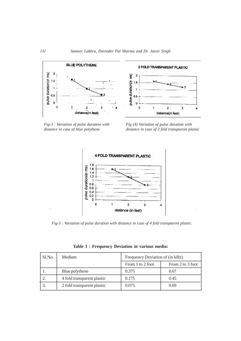
During the optimisation process the system was constantly monitored for performance bymeans of various evaluation options like spot size, ray aberration curves, modulation transferfunction and the field aberration. The RMS polychromatic spot size for zero, half and fullfields are 6.36µm, 6.38µm and 7.60µm respectively (Fig.4). The relative illumination for zero,

Figure-1 Figure-2

Ranabir Mandal and Ikbal Singh

237

half and full fields are 100%, 99.9% and 99.6% respectively, which means uniform illuminationover the whole field is achieved. Fig.5 shows RIM ray aberrations of the system. Finallyfig. 7 shows the polychromatic MTF curve of the objective.

FOCUS ADJUSTMENTDepth of focus is a critical parameter for any fast objective lens. The shift of back

focal length (BFL), with respect to different object distance is analysed and the result is shownin the fig. 7. It is found that if the system is focused at infinity, the shift of BFL due to the


238

object at 3 km, 4 km and 5 km are 66, 50, 39 micron respectively. The through focus spotof the system with object distance 4 km is shown in fig. 8. and through focus MTF is shownin fig. 9. The evaluation curves shows system will maintain diffraction limiting performancewith tolerable focal shift. Hence system focused for 4 km, can be operated for the rangefrom 3 to 5 km, without any defocusing problem.

Figure-8 Figure-9

CONCLUSIONSIn this paper, we have reported a new design configuration of a high aperture, long focal

length catadioptric objective for Long range passive night vision. It is to be pointed out thatthe conventional two-fold objective is compact but has a higher central obscuration, requiresbaffles and ray shade to avoid stray light. Though the designed system is not so compact incomparison to the conventional catadioptric objective, there is no need to use baffle to stopstray light. It has a relatively higher transmission as it uses only one primary mirror.

ACKNOWLEDGEMENTSThe authors are grateful to Mr. J.A.R. Krishna Moorty, Director, IRDE for his able

guidance and giving permission to publish this work.

Ranabir Mandal and Ikbal Singh

239

REFERENCES1. “Electro Optical Photograph of Low Illumination Level”, Soule H.V., NY, John Wiley &

Sons, 1968.

2. Scoping out Night Vision; NLECTC Bulletin, National Law Enforcement and CorrectionsTechnology Center, March 1996.

3. Long Range Night Vision system AN/PVS-8, Litton Electro-Optical Systems.

4. CODEV is a registered trademark of Optical Research Associates, California.

5. Night Vision Technology, DRDO Monographs, R. Hradaynath, 1999.


240

A SIX WATT SINGLE STAGE PULSE TUBEREFRIGERATOR OPERATING AT 77K

S. Kasthurirengan, S. Jacob, R. Karunanithi, D.S. Nadig, Upendra Beheraand M. Kiran Kumar

Centre for Cryogenic Technology, Indian Institute of Science, Bangalore 560 012, India

ABSTRACT

Cryocoolers have found a variety of applications in different areas such as, cooling ofInfrared detectors, Charge-Coupled Devices, SQUID magnetometers, Cryopumping etc.In particular, in the last two decades there has been significant technological developmentin the area of the Pulse Tube Refrigerators (PTRs), due to the absence of moving partsat cryogenic temperature leading to reduced mechanical vibrations and increasedreliability. Also, Pulse Tube refrigerators have achieved efficiencies quite comparable tothe other Cryocoolers such as Stirling, Gifford McMahon etc, and hence they areconsidered even for space applications.

Pulse Tube Refrigerators works on the principle that when a gas in the tube is compressedand expanded alternately, heat is transported from one end to the other in the direction ofcompression, due to the interaction of gas with the wall. The addition of regenerator and heatexchangers at the cold and warm ends of the Pulse Tube produces the refrigeration at thecold end. The Pulse Tube can either be directly coupled to the compressor, (this configurationis know as Stirling type PTR) or a pressure wave generator such as Rotary valve can beused between the compressor and the Pulse Tube, (this configuration is known as GMtype PTR).

The paper presents the design, performance characteristics and operational experiencesof a single stage Pulse Tube Refrigerator of GM type, which produces 6W of refrigerationpower at 77K. All the components of this system are indigenous except for the heliumcompressor of 3 kW capacity. The experimental results are discussed in the light of applications,where the temperature of the cold end needs to be maintained constant at different orientationsof the Pulse Tube.

1. INTRODUCTIONCryo-refrigerators operate at low temperature to produce the required refrigeration power.

Several types of cryocoolers based on different cycles such as GM, Stirling and Pulse Tubehave been used for a variety of applications. Some of the important applications are Sensorcooling, radiation shield cooling, cooling of superconducting magnets, cryopumping etc. Inthese systems, the high and low pressures (the discharge and suction pressures) from the


241

helium compressor is alternately connected at a specific frequency to the cold head by a rotaryvalve.

Of the different cryocoolers, Pulse Tube have been preferred due to the absence of movingparts at cryogenic temperatures, leading to their increased reliability and long term performance.

In a typical pulse tube cooler, the high and low pressures of the working gas are alternatelyapplied to the empty Pulse Tube through a Regenerator. Due to the heat pumping effect fromthe open end to the closed end of the Pulse Tube, refrigeration is produced. In this paper, wediscuss the development of a single stage Pulse Tube system which produces refrigeration of6 Watts at 77 K.

2. EXPERIMENTAL SETUPThe schematic of experimental set up is shown in Figure 1. The pulse Tube and the

Regenerator housings are made up of AISI 304 stainless steel. The dimensions of the Pulse

Fig. 1 : Schematic of single stage pulse tube cryocooler

A six watt single stage pulse tube refrigerator operating at 77k

242

Tube are 14mm o.d., 13.3 mm i.d. and 250 mm length, while those of the Regenerator are19mm o.d., 18.3 mm i.d. and 210 mm length. The heat exchangers and the flow straightnersare made of copper of electrolytic grade. The Regenerator matrix is made of stainless steelwire meshes of size 200 and contains approximately 2000 meshes.

The warm end of the Pulse Tube is connected to a heat exchanger through which coldwater is circulated to maintain it at ambient temperature. Both the Pulse Tube and theRegenerator are mounted to the top flange of the vacuum jacket by O-Ring seals. The coldends of the Pulse Tube and Regenerator ends in a copper heat exchanger with indium seals.

The Helium compressor serves as the source for high and low pressure gas supply tothe Pulse Tube. The pressure oscillations are generated by a Rotary Valve, which periodicallyconnects the high and low Pressure of the Helium compressor to the Pulse Tube. The rotaryvalve has been indigenously deveolped.

The design of the setup was such that the Pulse Tube can be operated either in basic, ororifice or double inlet mode with the help of needle valves (Swagelok make) along with astainless steel buffer volume of 0.5 litres.

PT100 sensors are mounted along the Pulse Tube and the regenerator to measure thetemperature at different locations as shown in figure 1. Four wire method of measurementhas been employed. Piezo electric pressure transducers (KPY47R, Siemens) are used to measurethe dynamic pressures at different locations.

The sensor outputs are monitored using a scanner and a DMM, which are interfaced tothe computer using IEEE 488 interface. Special software in C language enables online monitoringof the data.

The Pulse Tube and Regenerator are mounted inside a cylindrical vacuum jacket. Thevacuum jacket is fixed to a rotatable horizontal axle, by which the orientation of the PulseTube with respect to gravity can be varied from 0°to 180°. At the cold end of the PulseTube, a manganin heater of 62.5 Ω is fixed using GE varnish. Copper leads are used for currentflow, while manganin wires are used for voltage measurements. The heater can be energizedby using a power supply at constant current mode of operation.

The vacuum jacket is evacuated using a vacuum pumping system consisting of acombination of rotary and diffusion pumps.

3. EXPERIMENTAL RESULTS AND DISCUSSIONS

3.1. Cooldown behaviourThe typical cool-down behaviour in the double inlet mode for the 14mm Pulse Tube

operating at 2.3 Hz is shown in Figure 2. The lowest temperature obtained is 43.8 K, withDC flow correction a temperature of 38.3K is reached. Here S1 to S7 represent the sensorspositioned on the pulse tube and regenerator as shown in figure 1. Of the above, S5 is thecoldest, which is mounted on the regenerator bottom most position.

S. Kasthurirengan, S. Jacob, R. Karunanithi, D.S. Nadig, Upendra Behera and M. Kiran Kumar

243

3.2. Refrigeration Power of the Pulse TubeThe cooling power characteristics of the Pulse Tube can be estimated as follows. For a

given heat load applied through the heater at the end of the Pulse Tube, the steady temperaturereached at the cold end is monitored. The heat load is raised in known steps from 0 to 7W.The typical experimental results for the 14mm Pulse Tube is shown in Figure 3.

Fig. 2 : Cooldown behaviour of Pulse Tube Refrigerator

Fig. 3 : Cooling Power characteristics of single stage PTR


244

The system leads to a refrigeration power of 6Watts at 77K and nearly 8Watts at 100K.In general, DC flow correction leads to lower cold end temperatures and also increasedrefrigeration power at a given temperature. By using an improved heat exchanger at the coldend, a refrigeration power of 7W at 77K and 9.2W at 100K has been achieved recently.

3.3. Angular variation of cold end temperature of the Pulse TubeDue to the convection effects occurring in the Pulse Tube, the cold end temperature is

dependent on the orientation of the Pulse Tube with respect to the gravity. To study this effect,the Pulse Tube is positioned at different orientations and the cold end temperatures are measured.The typical angular variation is shown in Figure 4.

Fig. 4 : Angular variation of Cold End Temperature of PTR

The lowest temperature is observed at the zero degree angle (i.e. the cold end is at thelowermost position). On gradually increasing this angle, the cold end temperature rises slowlyup to the angle of 70°.

Further increase in the angle leads to larger increase in the cold end temperature. It reachesa maximum value at around 120°. Beyond this angle, the cold end temperature decreases. At180°( i.e. when the cold end is at the top most position) the cold end temperature is less butnot as low as that of zero degree orientation.

4. CONVECTION IN PULSE TUBESThe above behaviour is attributed to the convection phenomena occurring in the pulse

tubes. Thummes et al. [1,2] have shown that these convection effects can be reduced tosome extent either by increasing the frequency of pressure wave oscillations or by using suitableinserts (internal structure) within the pulse tube. Although the latter procedure decreased to


245

some extent the orientation dependence, the minimum attainable cold end temperature increasesconsiderably, simultaneously impairing the cooling power characteristics. Hence the presentexperimental studies have been directed towards a better understanding of convection inPulse Tubes.

The natural convection in fluid layer results from a temperature induced density gradientand the correlated buoyant forces due to gravity. The heat transfer by natural convection ischaracterized by Nusselt number defined by

Nu = (Qcon+Qm)/Qm (1)

Where Qm is the molecular conduction, Nu is a function of Raleigh number Ra and Prandtlnumber Pr. Qcon refers to the heat flow due to gas conduction. Ra is given as,

Ra(x) = g(Th-Tc)x3 Pr/ (γ2 <T>) (2)

Here g is the acceleration due to gravity, Th and Tc are the high and low temepratures atthe ends of the tube, x is the distance parameter and γ is the kinematic viscosity. <T> is theaverage temperature across the Pulse Tube.

Defining the angle between the gravity vector and the Pulse Tube as θ, Nu(θ = 0) is 1.For small angles of convection below 90° i.e. 2° < θ < 90°

Nu = 0.58[Ra(d)sinθ]1/5 (3)

With d as the diameter of the Pulse Tube. For angles between 100° to 180°

Nu = 1.44 + [Ra(L) cos(l80-θ) / 5830]1/3 (4)

In the above equation L refers to the length of the Pulse Tube.

Using these expressions, one can arrive at theoretical Nu and compare them with theexperimental data. Such a comparison shows the deviation of the theory from experimentalresults. It is observed that theoretical Nu is smaller compared to the experimental Nu. Thetheoretical Nu does not show a maximum with respect to the angle of orientation (as indicatedby experiment).

Towards the better understanding of convection effects, experiments have been carriedout with Pulse Tubes of different lengths and at different operating frequencies. Detailed analysisis underway.

5. CONCLUSION

In this paper, the development of single stage Pulse Tube refrigerator which is capableof producing 6W to 7W refrigeration at 77K is discussed. This system is entirely indigenousexcept for the Helium Compressor.

Currently, work towards the indigenisation of the helium compressor is in progress. Thepresent system will be extremely useful towards many applications such as sensor cooling aswell as studies of experimental samples at cryogenic temperatures in many laboratories.


246

REFERENCES1. G. Thummes, M. Schreiber, R. Landgraf and C. Heiden “Convective heat losses in

Pulse Tube Coolers: Effect of Pulse Tube inclination”. Cryocoolers I, Editor R. G. Ross Jr.Plenum Press New York (1997).

2. S. Kasthurirengan, G. Thummes and C. Heiden, “Reduction of Convectional HeatLosses in low frequency Pulse Tube coolers with mesh insert” Adv. In Cryogenic Engg.,45 (2000).

3. S. Kasthurirengan, G. Thummes and C. Heiden, “Elliptical and Circular Pulse Tubes:A Comparative Experimental Study” Proceedings of ICEC 18, Mumbai, India (2000)p.547

4. R. Karunanithi, S. Jacob, and S. Kasthurirengan, “Design and development of a SingleStage Double Inlet Pulse Tube Refrigerator”, Proceedings of ICEC 18, Mumbai, India(2000) p.539.


247

PROGRAMMED MICRO-INCREMENTAL HEIGHTPOSITIONING FOR SAMPLE CELL OF PARTICLE

SIZE ANALYZER

A.K. Pansare1 and A.M. Narsale2

Western Regional Instrumentation Centre, Mumbai - 400098Dept. of Physics, University of Mumbai, Mumbai - 400098

ABSTRACT

In photo-sedimentation method of particle size measurement of powdered material, samplecell scanning technique is normally used to reduce the measurement time. It is therefore,necessary to accurately position and move the cell in the optical system. A pre-programmed micro-incremental drive system has been designed which meet theserequirements.

The micro-step drive mechanism for the flow-through cell consists of a micrometer screw-head mechanically coupled to a high resolution stepper motor. The sample cell is movedby this system in vertical direction so that the cell traverses through the optical scanningsystem from bottom upwards. The cell holder assembly moves linearly through opticalsystem; the rotational component of the movement being eliminated by the groovedguides of the cell drive assembly. The limit switches at both ends prevent the systemfrom being overdriven. They also provide appropriate signals such as stop, ready,direction change, etc., for the electronic circuitry for the next sequential action to beinitiated. The total movement of the sample cell is 30 mm and is accomplished in 12,000increments, each micro-increment being 0.0025 mm. The sample cell is moved in pre-programmed steps by the main control and driver circuitry.

The paper discusses the design features and construction of the assembly. It alsodiscusses the driver and control circuitry used for the micro-incremental heightpositioning of the sample cell of the particle size analyzer.

1. INTRODUCTIONKnowledge of the size characteristics of particulate matter is generally of little value in

itself; but particle size measurements are often made to control the quality of the final product,because certain sizes may be correlated with certain desirable properties of the product.

Particle size distribution results are generally obtained in practice by counting and measuringparticles directly with a microscope or indirectly from the particle images on photographs, byelectronic counting and sizing as with the Coulter Counter, and by measuring sedimentation


248

rates. The sedimentation technique of particle size measurement is very often used, as it offersseveral advantages. It measures a rigorously defined dimension Stokes’ diameter (or equivalentspherical diameter). Sedimentation size analysis depends on the measured equilibrium velocityof a particle through a viscous medium due to gravitational force being related to the particleby Stokes’ law. The technique as normally practiced, is slow and the results are easilyinvalidated by temperature fluctuations and procedural disturbances. To minimize analysis timethe position of the sedimentation cell is continuously changed so that the effective sedimentationdepth is decreased with time. It is therefore, necessary to accurately position and move thecell in the optical system. In this photo-sedimentation method of particle size measurement ofpowdered material, the acquired data is presented as cumulative projected area versus Stokesianor equivalent spherical diameter, such that the equivalent spherical diameter indicated at anyinstant corresponds to the maximum equivalent spherical diameter at the depth where the beamis making the photoextinction measurement. To meet these requirements of accurately scanningand positioning the sample cell, a pre-programmed micro-incremental drive system has beendesigned.

2. BASIC PRINCIPLE OF THE DESIGNED INSTRUMENT:The photo sedimentation particle size analyzer designed for measurement of particle size

distribution of powder samples uses the gravitational sedimentation method together withphotoextinction method.

Sedimentation size analysis1 depends on the fact that the measured equilibrium velocityof a particle through a viscous medium, resulting from the action of the gravitational force,can be related to the size of the particles by Stokes’ law.

For spherical particles, Stokes’ law for sedimentation is expressed as:

18 η hD = -------------- x ---- , where (ρ - ρo)g t

D is the diameter of the particle, v is the sedimentation velocity of the particle, given byh / t, h is the sedimentation height, t is the sedimentation time, ρ is the sample density, ρ

O is

the density of the fluid, η is the viscosity of the fluid, g is the acceleration due to gravity.

From the above Stokes’ law of sedimentation, for a sample of known density and a liquidof known density and viscosity, the Stokes’ diameter can be easily obtained if the sedimentationheight and the time required to travel that height are accurately measured. The time requiredto measure fine diameter particles in normal sedimentation process is inherently very large.Hence, to reduce the measurement time and to cover a wide range of particle size distribution,scanning of the sedimentation cell is necessary. In this technique, the sedimentation height iscontinuously reduced in a programmed manner, such that at any time the sedimentation heightis accurately known. The measurement time is thus, drastically reduced from hours to about20 minutes, for a typical sample.

The need for accurate micro-positioning of the sample cell, therefore is highly essentialif the results obtained from the instrument are to be accurate, and reliable and the measurementtime is to be drastically reduced. The designed micropositioning system for the sedimentationcell meets these requirements.

A.K. Pansare and A.M. Narsale

249

3. DESIGN FEATURESThe mechanical assembly of the sample cell drive system is shown in figure 1. The drive

mechanism for the flow-through cell consists of a micrometer screw-head driven by a high

Fig. 1 : Mechanical assembly of the sample cell drive system

resolution stepper motor requiring 200 pulses for one revolution with a rotational angle of 1.8degrees per step. The total linear displacement of the sample cell is 30 mm. This distance iscovered through the drive mechanism of the system in 12,000 increments, each incrementtherefore, being 0.0025 mm.

The control and the timing section of the instrument, as shown in figure 2, decide theprogrammed pulsing rate for the stepper motor. Since the incremental step size is known, thesedimentation height that relates to the position of the cell, can be easily determined fromwhich the Stokes’ diameter (equivalent spherical diameter), can be accurately calculated. Usingthe scanning technique, the measurement time is drastically reduced from hours to minutes.

The micropositioning system is highly accurate. There is minimal backlash thereby ensuringthat the positioning of the cell is highly accurate and reproducible. The unislide guides on thesides of the cell holder ensure that the cell moves only in the vertical direction and the duckingand wobbling of the cell is kept to the minimum. To ensure that the sedimentation process is

Programmed micro-incremental height positioning for sample cell of particle size analyzer

250

taking place undisturbed, the vibrations due to the stepper motor are minimized by havinganti- vibration cushioning for the cell mounting. Further, the vibrations, due to the peristalticpump used for circulation of the sample through the cell, are minimized by having the pumpassembly mounted on a specially designed anti-vibration mounting.

Mounted on the drive is the sample cell holder. The cell holder has a unique locking featurethat locks the cell in the holder so that every time the position of the cell is reproducible.

The micro-limit switches at the top and the bottom ensure that the cell movement isrestricted to within the limits. The bottom switch is activated at the end of the scan, the directionof the stepper motor is reversed and the motor reset at a higher pulse rate. When the cellreaches the top i.e. home position, the top limit switch is activated, the motor is stopped andthe direction of the motor again reversed. The system is now ready for the starting of thenext analysis. For accurate calibration of the position of the cell at the beginning of the analysisand at the end of the scan, there is a provision for fine adjustment of the positions of both thelimit switches that ensures correct starting and stopping of the stepper motor.

4. DESIGN OF THE CONTROL CIRCUITRY :The control circuitry of the driver section generates the appropriate code sequence required

for the stepper motor2,3,4. This section also sets the correct direction of rotation of the motoras decided by the program during the normal analysis and during resetting of the stepper motorat the end of the analysis. Higher stepping rate is used during the reset operation to return thesample cell to it’s home position at the fastest permissible speed. The electronic driver circuitryfor the stepper motor consists of power transistor stages for driving the high current motorwindings. Pre-amplifier driver stages are used to the meet the power requirements. A separate

Fig. 2 : Block schematic diagram of the sample cell drive system

A.K. Pansare and A.M. Narsale

251

printed circuit board has been designed for the stepper motor driver circuitry. It has beenconnected to other circuits; through appropriate connectors. The layout of the system hasbeen designed in such a manner that it enables easy hardware debugging by having test pointsand signal injection points. These features considerably aid during fault diagnosis. Figure 2shows the block schematic diagram of the sample cell drive system.

Across each motor winding protection diodes are used to suppress the EMI likely togenerated by the back-emf during the switching of the high currents in the motor windings.Separate high current/high voltage power supply has been designed for the stepper motor soas to reduce interference with the low current/low voltage power supply used for sensitivedigital and analog circuitry.

5. CONCLUSIONSThe described system is a subsystem of particle size analyzer used for measuring particle

size distribution of powdered samples. The design of the system enables the accurate positionof the sample cell, so that the sedimentation height can be easily determined. From thesedimentation height the Stokes’ diameter is obtained. The accuracy of the positioning of thesample cell is evident from the high reproducibility of particle size distribution results of thesame sample repeated at different times. The blank sample cell scan (base line check) alsoyields a straight line and is highly reproducible. The measurement time for a typical sample isdrastically reduced from hours to about 20 minutes. The design enables reproducible andrepeatable positioning of the sedimentation cell. The cell loading and cleaning process is alsogreatly simplified. The measure of the performance of the designed system is the high accuracyand reproducibility of the results obtained from the instrument.

REFERENCES1. Particle Size Measurement, Vol. I, Terence Allen, Fifth Edition, Chapman & Hall, London, 1997.

2. A Microprocessor stepping-motor controller – B. G. Strait, M. E. Thout, Microcomputer design& applications, Edited by S. C. Lee, Academic Press, London 1977.

3. Stepper motor drive, and (ii) State generator for stepper, John Markus, Charles Weston,Essential Circuit Reference Guide, McGraw - Hill Book Co., 1988.

4. Microprocessors & Interfacing - Programming & Hardware, V. Hall, 2nd Edition, Macmillan /McGraw-Hill School Publishing Co. 1992.

Programmed micro-incremental height positioning for sample cell of particle size analyzer

252

ON-LINE PROCESS CONTROL UNIT FOR JAGGERYMANUFACTURING INDUSTRY

S.T. Pawar and M.B. DongareDepartment of physics, Shivaji University, Kolhapur-416004

ABSTRACT

Agriculture and agro-based industries form the backbone of Indian economy but theyare still adopting traditional methods. Jaggery industry is an important agroprocessingindustry in rural lndia. The major constraint in this industry is lack of standardisation inprocessing. In traditional method of jaggery manufacturing a so-called skilled personknown as “Gulvaya” plays a deciding role in clarification of sugarcane juice and inconfirming formation of ‘Kakavi’ (liquid jaggery) and jaggery. The presently developedmicrocontroller based on-line process control unit is field usable and can give audioindication of important parameters (pH and temperature) and display the parameters indecimal form on the LED numeric display. It has resulted in giving us a precise results,in order to produce a superior quality jaggery. Key words:-Development of process controldevice in jaggery industry.

1. INTRODUCTIONIndia is the largest producer of sugarcane in the world occupying about 4.0 million-hectare

of land. The area in which sugarcane is grown in Maharashtra is 601 thousand hectares andis 11.1% of the total area in which sugarcanes grow in India. The yield is 82394 kg/ha1. InIndia total sugarcane production is of 227.06 lak tonnes. Out of total sugarcane production43.5% is used for jaggery and khandari2. About 10.3 million tonnes of jaggery is producedannually in India7. The major constraint in jaggery industry is lack of standardisation inprocessing. In addition an unhygienic surrounding during manufacturing, packaging and storageare major problems.

2. EXPERIMENTAL DETAILSThe field experiment was conducted from Nov 2000 to March 2001. From our study

and field survey of 25 jaggery-manufacturing units in western part of Maharashtra, it hasbeen noted that, temperature and pH plays an important role in manufacturing process ofjaggery. Whatever may be the initial Brix of the cane juice the two important striking pointsare appearing at a fixed temperatures only. viz. Liquid jaggery (Kakavi) at 105°C and finalstriking stage (Golli stage) at 118°C Also it has been noted that initial pH of juice varies from5.1 to 5.7. For clarification it is raised by the use of lime water to 5.9-7.00. The neutrilisation


253

is achieved by use of chemical clarificants. The observed range of pH after neutrilisation is4.8 to 5.4. These are the variations due to manual and approximate use of clarificants. Theseleads to variation in quality of jaggery.

It is also found that for extra-special (Extra) and grade no.l jaggery the correspondingincreased and decreased pH values are to be 6.3 and 5.3 respectively.

Thus quality of jaggery is influenced by physical parameters like pH and temperature3.Hence there is a need of on-line field usable process control unit to be developed to meet therequirement of farmers to get superior quality jaggery. Some of the novel features of thedeveloped system are set point facility to meet region-wise variation in parameters and churnercontrol.

3. ON-LINE PROCESS CONTROL UNIT FOR JAGGERY MANUFACTURINGINDUSTRY

The developed microcontroller based on-line process control unit is designed specially tomeet the needs of farmers. The system incorporates pH electrode and temperature sensor todisplay and give the audio indication of important stages in jaggery manufacturing process,The system is user friendly and does non-destructive measurement.

3.1 Hardware of the SystemThe developed system consists of (H2C12) Calomel electrode, an instrumentation amplifier

(LM 321), temperature transducer (pt 100), constant current source formed by LM 324 andBC 557, ADC 0809 Board and microcontroller 89C51. The system can measure pH valuewith an accuracy of 0.1 of the reading, The system is energized by a highly regulated powersupply. The block diagram of the system is shown in Figure. l.

Fig.1 : Block diagram of microcontroller based on-line process control unit

On-line process control unit for jaggery manufacturing industry

254

3.2 pH ElectrodeTo obtain an accurate measurement of the emf. developed at the electrode, the electronic

measuring circuit must have a high input impedance. The developed emf, is suitably amplifiedby the instrumentation amplifier before applying it to the ADC. When the combined electrodeis immersed in a solution, a potential is developed. This potential is actually very small of theorder of few millivolts.

3.3 PT-100 RTD SensorAs compared to Nickel and Copper, platinum has been found to be relatively linear within

the specified range. The platinum further has additional merits, which make it suitable for thepresent application. These merits are – 1) high precision and accuracy 2) Ease of calibration3) high responsibility 4) fast response 5) Interchangability with other resistance without anycompensation 6) Good performance in desired temperature range and 7) limited susceptibilityto contamination etc. Pt-100 is two terminal passive sensors. It has wide measuring range –100OC to 600OC.

3.4 Instrumentation Amplifier (LM 321)Op-amp LM321 and opamp LM324 ICs are connected in the non-inverting mode and

are used to amplify the millivolt signal generated by the pH electrode.

3.5 A/D Converter InterfacingADC 0809 is a monolithic CMOS device with 8-bit ADC. It uses successive approximation

as the conversion technique. ADC 0809 is a 8 – channel ADC for unipolar analog signals6.

3.6 MicrocontrollerMicrocontroller 89C51 is used to process the input data with setpoint values of temperature

and pH. The 89C51 have the following features :

l. Eight bit CPU with accumulater A and B registers.

2. 16 bit program counter and data pointer.

3. 8 bit stack pointer.

4. Internal E2PROM of 4K.

5. Internal RAM of 128 bytes.

6. 32 I/O pins arranged as four 8-bit ports.

7. Two 16 bit timer/counter.

8. Full duplex serial data transmitter / receiver.

9. Control registers TCON, TMOD, SCON, PCON, IP and IE.

10. 2 External and 3 Internal interrupt sources

11. Oscillator and clock circuits.

According to the selected data, the appropriate control signals are generated and are appliedto the buzzer and motor drive unit.4

S.T. Pawar and M.B. Dongare

255

3.7. 7447 display drives / decoder and key board

7447 is display driver for common anode type seven segment displays. Keyboard is usedto set the initial and final set points related to desired pH and temperature values.

4. SOFTWARE OF THE SYSTEM

In microcontroller based system, software design is a more demanding task than hardwaredesign. The software is written in assembly language of microcontroller 89C51 to performthe following :

l. Analog to digital conversion program

2. Display program for pH and Temperature

3. Data byte of pH and Temperature

4. Delay program

5. CALIBRATION AND WORKING

Using standard laboratory pH meter and thermometer carries out the calibration of theunit. The pH electrode and temperature sensors are placed in the sugarcane juice- boilingpan. The power is supplied to the system by means of the stabilized IC regulated dcpower supplies.

The analog outputs from the transducers, after suitable signal conditioning, amplificationand conversion are applied to the channels of the ADC 0809. Here channel 0 is used. ADC0809 convert’s analog inputs into digital outputs in hex from by executing the main program.The digital values arc processed by microcontroller 89C51 and pH and temperature valuesfor cane juice under process are displayed. The unit gives audio indication in accordance withpreset values of pH and temperature. It also controls the churner action in jaggery manufacturingprocess.

6. TESTING OF PROCESS CONTROL SYSTEM

The performance of the unit has been successfully tested at 10 jaggery- manufacturingunits in Kolhapur region. During test we have carried out the jaggery preparation by makinguse of process control device. Irrespective of soil type and sugarcane genotype we haverecorded the recovery and grade of the jaggery.

System Setting -

I) pH was set at 6.3 for lime defection and at 5.3 for neutralization.

II) Temperature was set at 105OC. for liquid jaggery (Kakavi) stage and at 118 C. forjaggery (Golli) stage. Table-1 gives the result of 10 jaggerymanufacturing units in Kolhpurregion.


256

Jaggery Unit No. Jaggery Recovery Jaggery Grade*

1 10 Extra

2 11 1

3 12 Extra

4 11 1

5 10 Extra

6 12 1

7 11 1

8 10 Extra

9 11 1

10 11 Extra

* Grade of jaggery is recovered as per present jaggery grading method adopted in jaggerymarket. Any market does not follow scientific grading method. In market gradingis done by physical appearance of jaggery i.e. by checking test, color and hardnessby knife (Granular size).

* The grade numbers given by jaggery market are :

1. Extra special grade (extra)

2. Grade no-1

3. Grade no-2

4. Grade no-3

5. Grade no-4

6. Grade no-5

The jaggery of the grade i.e. Extra and grade no-1 fetches maximum price in market.

7. CONCLUSIONThe observed results reveal that the microcontroller based on-line process control unit

for jaggery industry is sufficiently accurate in monitoring physical parameters of sugarcanejuice. The unit gives better result as compared to manual judgement by a person known as“Gulvaya” in jaggery manufacturing process. This unit is highly beneficial to the farmers indeciding the two important striking stages and it helps in optimum clarification so that a goodquality jaggery can be produced. From Table-1 we found that the jaggery recovery rangesfrom 10-12 and grade of product is maintained between extra-special (extra) and grade-1.

ACKNOWLEDGEMENTOne of authors (STP) is thankful to University Grants Commission, New Delhi for award

of teacher fellowship under FIP.

Table 1 : Results of 10 Jaggery manufacturing units in Kolhapur region

S.T. Pawar and M.B. Dongare

257

REFERENCES :1. Damahe, B.A. 14(2000). Application of I.T. in area of Agri. And Agrobased industry. Proc.

Seminar on INFOTECH.

2. Patil, J.P. et. al. 1-3 (1996). Research bulletin on liquid jaggary MPKV. RES. PUB. NO. 17.

3. Pawar, S.T. et. al., 369-374 (2001) Scientific studies on Jaggery Manufacturing process. Co-operative Sugar Vol-32, No. 5.

4. Kenneth J. Ayala. 54-60 (1996). The 8051 microcontroller Architecture, programming andapplication. Second edition. Penram International publishing (India).

5. Raman K. Attri et. al., 275-283 (2000) Design Approach to use Pt RTD sensor. J. Instrum.Soc. India 30(4).

6. B. Ram. (1995). Fundamentals of microprocessor and microcomputers. 4th edition. DhanapatRai Pub. Nai Sarak, Delhi.

7. Dorge, S.K. I-II (1994). Proc. of National consultation meeting feb. 27-28 : RS and JRS,Kolhapur.


258

DEVELOPMENT OF AUTOMATIC AIR SAMPLER

S. Chellammal, G. Surya Prakash, R. Mathiyarasu and K. M. SomayajiAtmospheric Studies and Radiation Instrumentation Section

Health And Safety Division, SHINE Group Indira Gandhi Centre for Atomic Research,Kalpakkam, 603 102

ABSTRACT

In a nuclear facility, it is essential to assess and predict the radiological consequencesto public during routine operations. Atmospheric dispersion models are used for thestudy of dispersion of radioactive releases to the atmosphere, which requires validationfor operational use. The ambient concentrations of a pollutant can be measured at differentdistances from source in the downwind sectors, which requires a large number of airsamplers to be deployed. To achieve this, a portable, programmable air sampler wasdesigned and developed for simultaneous and automatic sampling. The systemdescription and function are discussed in this paper.

1. INTRODUCTIONIn a nuclear facility, dispersion calculations are needed in order to determine the impact

of radioactive releases, normally released from stack, to the environment. Atmosphericdispersion models, considering parameters over Kalpakkam coastal terrain due to land-see breezeeffects have been developed. Validation of the models requires data sets including experimentalresults of dispersion experiments and simultaneous meteorological measurements of the windand turbulence field. Dispersion experiments can be performed with sulfur hexafluoride (SF6)as tracer. The ambient concentrations of the tracer should be measured at different distancesfrom source in the downwind sectors, which requires a large number of air samplers to bedeployed.

The conventional air samplers used in pollution control studies sample only the pollutantson filters, which is used for further analysis. Whereas air samplers used in tracer experimentscollect and bottle up known volume of air along with unknown quantity of tracer in ”tetler”bags of known capacity with known flow rate.

A tracer release experiment was conducted by Forschungszentrum Julich GmbH (KFA)group for assessing dispersion characteristics around their nuclear facility using similar airsamplers. The tracer sampling units built by KFA group are based on sampling of air in plasticbags. Each unit can collect 3 samples, starting from a prefixed time and running for fixedselectable consecutive time intervals. Air sampling units constructed by another Danish tracer-group are also based on sampling air with flow rate of 200 ml/min in three plastic bags attachedto the outlets of a box.


259

These air samplers are electro-mechanical in nature and huge manpower was used duringexperiments. Further, synchronization of different sampling units was difficult. So, to meetthe operational logistics with reduced manpower, portable, battery operable and programmableair sampler was designed and developed at Health and Safety Division, SHINE Group, IGCAR.The sampled air will be analyzed for concentration measurement of the tracer using gaschromatograph technique.

2. SYSTEM DESCRIPTIONThe block diagram of the system is as shown in Figure l. It consists of a Sampling unit Microcontroller based control unit. The system is preprogrammed with PC before

its deployment in the field.

Fig. 1 : Block Diagram of Automatic Air Sampler

Development of automatic air sampler

260

2.1. Sampling UnitIt consists of a miniature pump along with three pulse operable latching type solenoid

valves. The pump has a delivery capacity of 0.85 litres/minute. The pump outlets are connectedin parallel to three solenoid valves. The atmospheric air drawn through the pump is sequentiallyswitched through solenoid valves to three sampling bags. The flow rate of the system hasbeen adjusted such that a typical sampling bag of 10 litres capacity gets filled upto 8 litres inabout 30 minutes. These are typical values in atmospheric air sampling during tracer releaseexperiments.

2.2. Microcontroller based control unitThe control unit is based on an industry standard microcontroller (Intel 80C31), an EPROM

(32k, Intel 27512), a Real Time Clock (RTC MC 146818) and electronics to control valvesand pumps. The necessary control/system program is written using assembly language of80C31 instructions, assembled, linked and stored in Intel-hex format in EPROM. The controlunit is connected to PC through RS 232 port.

2.3. User InterfaceUser interface program is written in both QBASIC (DOS based) and Visual Basic (Windows

based) and it is PC resident. It provides the user a menu with options to

1. select communication port

2. enter initialization time of RTC

3. enter preset time of sampling

3. SYSTEM FUNCTIONSystem function is shown as a flow chart in Figure 2. As soon as the instrument is made

operative, control program ensures that, the condition of solenoid valves are normally closedand performs a system check of microcontroller. Normal functioning of the system is indicatedby a slow flashing of LED of about 5 times and LED goes OFF. Then the system programwaits for user command from PC. A user can enter the initialization time for RTC and onreceiving initialization time, control program will initialize RTC and makes LED ON. Now theuser can enter the preset time of sampling and on receiving the preset time, it is written intoRTC alarm locations. The RTC has a feature of comparing the real time with set alarm timeevery second and sets interrupt if both are equal. Using this feature, once the set alarm timeis reached, microcontroller sends control signals to microsolenoid valves and pumps as perprogram sequence. The waiting mode for the alarm is indicated by LED flash at 1Hz rate.After the sequential switching is over, pump is made OFF and system LED returns to slowflashing.

It may be noted that single LED indicates the various states of the system as follows.Initial system check by slow flashing,

Waiting for initialization of RTC time by LED off,

Waiting for initialization of preset time by LED on and

Waiting for alarm signal by LED flashing at 1Hz rate.

S. Chellammal, G. Surya Prakash, R. Mathiyarasu and K. M. Somayaji

261

Fig. 2 : Flow Chart of System Function

Development of automatic air sampler

262

4. GENERAL FEATURESThe system operates on 12 volts maintenance free rechargeable battery. Use of low power

ICs has enabled the current consumption of the system to a mere 90mA when the pump isrunning. The complete system is housed in an IP 64 instrument box, which does not allowinterference from ambient conditions during field deployment.

5. CONCLUSIONA programmable air sampler was designed for collection of air samples in Tracer

experiments being conducted for atmospheric dispersion studies. The instrument is testedsuccessfully for intensive field-sampling, system performance under battery operations. Afterseveral trials, the flow rate of the system has been adjusted such that a typical sampling bagof 10 litres capacity gets filled up to 8 litres in about 30 minutes. The unit is now ready inlarge numbers to be deployed during tracer release experiments. SF6 will be used as the tracer,which is a chemically inert and non-toxic gas. There are no natural and only few man-madesources of SF

6. Not only air, these samplers can also be used to collect any other gas. The

air sampler designed here is quite different from other conventional electro-mechanical airsamplers and it collects a specific volume of air along with tracer at different locationssimultaneously by PC software before deployment. Further, synchronization of differentsampling units has been made easier with programmable capability of the system. The air orgas samples are analyzed for tracer concentrations using gas chromatograph technique.

ACKNOWLEDGEMENTSThe authors wish to thank Dr. S. M. Lee, Director, SHINE Group and Dr. A. Natarajan,

Head, HASD for their encouragement and interest in this project.

REFERENCES1. Vob.W, 1993 SF6-Tracer measurements by KFA-Group in Fourth Field experiment on

atmospheric dispersion around the isolated hill sophienhoe in September 1989 Methods-Experiments-Data bank edited by G.Zeuner and K.Heinemann, p25-28

2. Lyck. E, 1993 SF6-Tracer measurements by NERI-Group in Fourth Field experiment onatmospheric dispersion around the isolated hill sophienhoe in September 1989 Methods-Experiments-Data bank edited by G.Zeuner and K.Heinemann, p29-38

3. Mortensen, N.G. and Gryning, S.E.: The Oresund Experiment: Databank Report, Dept.Meteorology and Wind Energy, RISO, Denmark, ISBN 87-550-1592-1, (1989).

4. Somayaji K.M, Mathiyarasu.R, Chellammal.S and Surya Prakash.G, ”Design and Developmentof a programmable Air Sampler” IGC Report-215, published by Indira Gandhi Centre for AtomicResearch, DAE, Kalpakkam, p 1-8, (1999)

5. Vob.W, Zeuner.G Tracer release and sampling network in Fourth Field experiment onatmospheric dispersion around the isolated hill sophienhoe in September 1989 Methods-Experiments-Data bank edited by G.Zeuner and K.Heinemann, p21-24.

S. Chellammal, G. Surya Prakash, R. Mathiyarasu and K. M. Somayaji

263

THE EFFECT OF SWIRL ON A TURBINE METER INAIR FLOW AND THE EFFECTIVENESS OF A FLOW

STRAIGHTENER IN REMOVING THE SWIRL

Mohd Islama, M.M. Hasanaa, S.N. Singhb and V. Seshadrib

aMechanical Engineering Department, Jamia Millia Islamia,New Delhi-25b Applied Mechanics Department, IIT, Delhi-16

ABSTRACT

Turbine Flowmeter (TFM) is being used extensively in various industries to measure theflow rate of wide variety of fluids due to its excellent repeatability, higher accuracycompared to other mechanical flow meters, wide operating range, higher shock capabilitycompared with electro-mechanical flowmeter, low pressure loss and can operate underadverse conditions of temperature and pressure. Turbine Flow Meter performance isdependent on upstream flow conditions, fluid properties and geometrical parameters ofrotor. In this study, the turbine flow meter performance has been evaluated for co andcontra direction upstream swirl flow. Swirl magnitude in both directions has been variedfrom 0°- 50° and it is seen that linear range of the meter factor is not significantly affectedfor co-swirl where the stopping flow decreases. For contra-swirl the trends for linearrange show similar behavior till 30° swirl flow but stopping flow increases. It is alsoobserved that meter factor is high for co-swirl and low for contra-swirl in comparison tozero swirl meter factor.

Notation:K - Meter factor, Pulse/m’TTS - Tube type straightenerWS - Without straightenerY - Distance from the wall of pipe in radial direction, mmα - Vane angle of swirler, degrees

1. INTRODUCTIONTurbine Flow Meters (TFM) today have been accepted as a highly accurate instrument

of flow rate measurement in various industries. The reason for their wider acceptance inthe industry is the accuracy, repeatability, wide operating range, ease of installation andelectrical output.

The present day Turbine Flowmeter was developed by Lee and Karlby1 after 7 year ofextensive research in 1960. Since then researchers have been extensively trying to improveperformance. Other important studies on TFMs are those of Lee and Evens2 and Thompsonand Grey3. They have tried to analyse the effect of geometrical and dynamical parameters on


264

the performance of TFM theoretically. Shafer4 described the general performancecharacteristics of TFM for liquid hydrocarbon in the range of 0.5 to 250 gpm. Salami5 hasconducted experiments on commercially available TFM having large tip clearance at rotor .Lee, Blakeslee and White have reported accurate measurement of flow rate by developing anew metering concept of self correcting and self checking TFM. Satyanarayana7 hasexperimentally investigated the effect of fluid properties on the TFM performance using waterand oil. Islam, Seshadri and Singh8-10 have investigated the effect of upstream skewed velocityprofile on the performance of a small gas TFM and found that only highly skewed upstreamvelocity profile changes the usable range and meter factor. Same authors have also investigatedthe effect of geometrical parameters of the rotor for improving the linear range of the TurbineFlow meter. Salami has clearly identified different parameters which are responsible in affectingthe meter performance and one of them is swirl, which is induced from normal pipe fittingsin an industrial pipe line. Investigation of swirl flow have in general been done with flowstraighteners and no one would sensibly use a turbine flow meter in a flow which is knownto be highly swirling and the requirement is to know the effectiveness of flow straightenersand the required dimensions – upstream spacing, length of straightener, distance fromstraightener to turbine meter to ensure that the meter performs within specification. In thepresent investigation an effort has been made to quantify the effect of swirl on the meterperformance in the absence of any flow straighteners and with tube type straightener. Upstreamswirl has been imposed in both co and contra direction of the rotor rotation of the TFM.

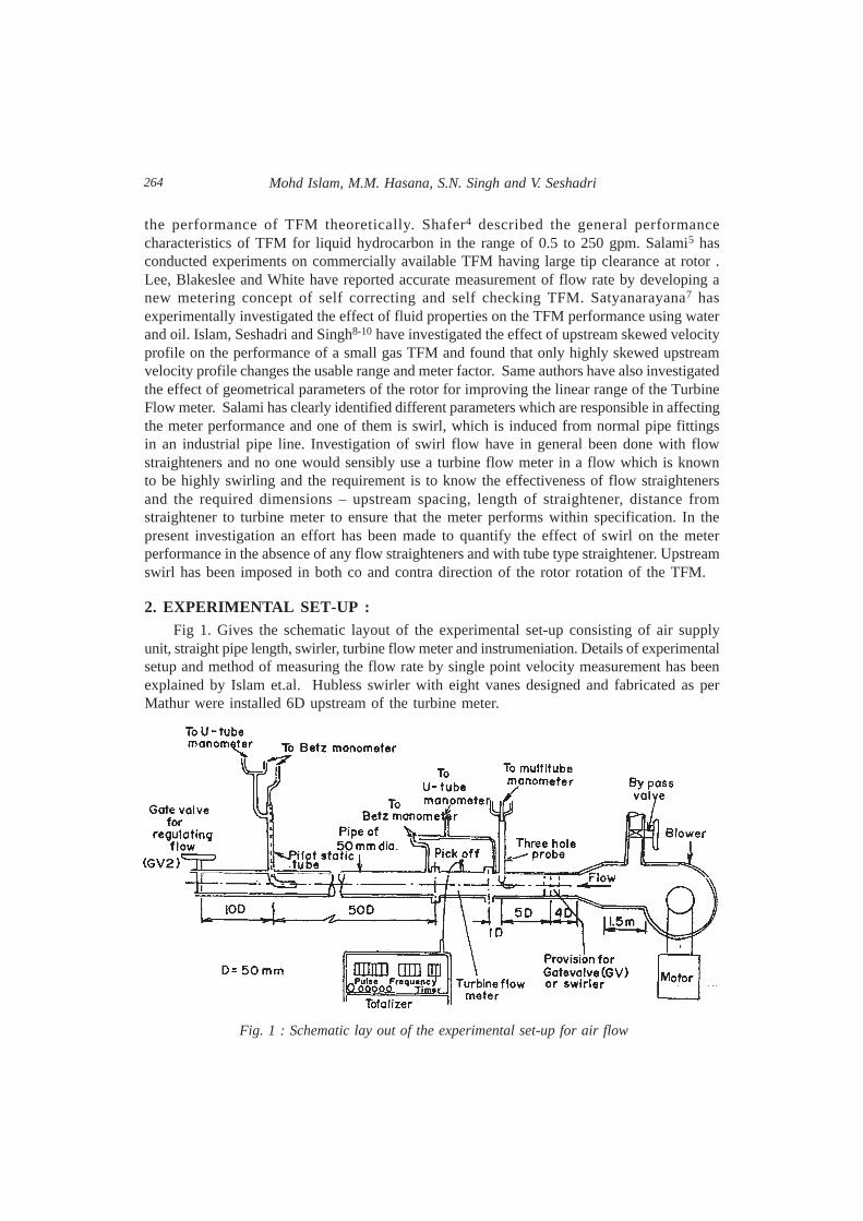
2. EXPERIMENTAL SET-UP :Fig 1. Gives the schematic layout of the experimental set-up consisting of air supply

unit, straight pipe length, swirler, turbine flow meter and instrumeniation. Details of experimentalsetup and method of measuring the flow rate by single point velocity measurement has beenexplained by Islam et.al. Hubless swirler with eight vanes designed and fabricated as perMathur were installed 6D upstream of the turbine meter.

Fig. 1 : Schematic lay out of the experimental set-up for air flow

Mohd Islam, M.M. Hasana, S.N. Singh and V. Seshadri

265

TFM as shown Fig. 2 supplied by Rockwin Flow Meter (India) Pvt.Ltd., was fitted inthe setup at the distance of 10 D down stream from reducer. TFM used in the presentinvestigation is the same as used by Islam et.al. and the details of which are given below.

a) Rotor diameter - 44.3 mm

b) Casing inner diameter at rotor - 44.8 mm

c) No. of blades - 6

d) Rotor shaft diameter - 4mm

e) Weight of rotor - 27.7358x10-3 kg.

f) Blade thickness - 1.3 mm

g) Blade angle from axis of meter - 30 degree

h) Span length of blade – 15 mm

The extent of swirl which could be generated by the swirlers was 10’ to 50’ on the averagein both co and contra direction. Range of parameters investigated is given in Table 1.

Table 1: Range of parameters investigated

Parameters Range Configuration Remarks

Upstream swirl 0°, ±10°, ±20°, Without Angle referred±30°, ±40°, ±50° straightener, with are the vane

tube type angle of swirlerstraightener with axial flow

direction

3. RESULTS AND DISCUSSIONSThe velocity profile ID upstream of the meter was measured by a pre calibrated three

hole probe (THP) in null mode and results are depicted in fig-3. Fig 3(a) depicts that the

Fig. 2 : Turbine flow meter with tube type straightener (Design 1)

The effect of swirl on a turbine meter in air flow

266

velocity distribution is symmetric about the center-line for all swirlers. It is clear from fig3(b) and (c) that for low vane angle swirlers, the swirl angle is almost constant across thepipe cross section and is equal to the angle of the vane except at center where there is aninflexion point.

In the present investigation for each combination the meter factor and pressure drop acrossmeter have been measured for co and contra swirl with tube type straightener and withoutstraightener. Figure 4(a) shows the variation of meter factor for undisturbed flow. It is seenthat meter factor remains constant as long as the flow rate is above 45.0 m3/hr for TTSallowing tolerance level of t 1% for usable range. This limit of usable range for withoutstraightener is higher because of the hump formation at low flow rate, which exceeds thelinearity band of 1% of the average meter factor. The hump formation can only be explainedin terms of resonance between rotor frequency and shedding frequency of the rotor wake.Hump is generally formed but its magnitude appears to be higher in the absence of straightener.Fig 4 (b) depicts the pressure drop across the TFM for undisturbed flow conditions. It isseen from the plot that the variation is similar but for without straightener it is lower becauseof the reduced blockage (approximately by 10%) within the meter.

Fig. 3(a) : Velocity distribution upstreamof TFM for different swirlers

Fig. 3(b) : Variation in angle for swirlerfor co-swirlers up stream of TFM

Fig. 3(c) : Variation in angle of swirler forcontra-swirlers upstream of TFM


267

Fig. 5 (a), (b), (c), (d), (e) show the variation of meter factor for co-and contra-swirl,with tube type straightener and without straightener with flow rate. It is seen that meter factorfor co-swirl is higher and for contra-swirl is lower than that for standard flow conditions(undisturbed flow condition). It is also seen that the shift in the meter factor for withoutstraightener is more than that for TTS. The shift in the meter factor can be attributed to therelative change in the driving and retarding torque due to increase of flow incidence angle forco-swirl and reduced incidence angle for contra-swirl. The increase in the driving torque forco- swirl is quite rapid which causes the rotor to rotate at higher speed to achieve equilibriumcondition. The same equilibrium condition is reached earlier for contra swirl and hence themeter factor is lower. It is quite evident from the graphs that as angle of swirler increases in

Fig. 4(a) : Characteristics of TFM for undisturbed flow conditions.

Fig. 4(b) : Pressure drop across TFM for underdistrurbed flowconditions.


268 Mohd Islam, M.M. Hasana, S.N. Singh and V. Seshadri

269The effect of swirl on a turbine meter in air flow

270

co-direction, the magnitude of hump formed increases for without straightener, but it remainswithin the ± 1% linearity band of the average meter factor till 30 degrees. For 40° vane angleswirler, the hump formed is quite significant and does not lie in the ± 1% linearity band andhence the usable range decreases.

Fig. 6 & 7 show the variation of pressure drop across the meter for all swirlers as afunction of flow rate for TTS and without straightener respectively. It is seen from the figurethat variations in pressure drop with different swirlers are similar in nature with and withoutthe straightener. Further it is also clear that the pressure drop increases with increase in theangle of swirler irrespective of direction of swirl. The extent of pressure drop is only marginallyaffected by the presence of straightener.

Fig. 8 (a), (b), (c) and (d) present the cross plots to clearly bring out the effect of swirlon the basic performance parameters. Fig 8 (a) shows that the average meter factor varies ata rate of about 0.086% per degree of swirler for TTS and 2.25% per degree of swirler forWS. This value is higher than the value quoted by Salami (5) and lower than the value quotedby shafer (4). Fig. 8(b) shows that in the presence of TTS lower limit of the linear range isalways lower than that WS. Similar observations were made by Salami (5), for lower valuesof swirl. Fig. 8 (c) shows that stopping flow for TTS remains within ± 1.7% of standardresult. In the case of without straightener, there is large variation for co and contra mode ofswirl. It is seen from the Fig. 8 (d) that average pressure drop coefficient is almost linearlyincreasing with the vane angle of swirler (for both modes) till 40° but it increases more rapidlybeyond 40°. It is also seen that in the case of the TTS pressure drop coefficient is alwayshigher than that of WS. This is expected because in presence of flow straightener there ishigher-pressure drop.

4. CONCLUSIONFrom the present investigation it has been found that meter factor increases for co-swirl

and decreases for contra swirl flow. Pressure drop across the meter increases in both casesof swirl. The usable range remains approximately constant till ±20° for without straightenerand till ±30° with the use of tube type straightener. The lower limit of the linear range fortube type straightener is always lower than that without straightener.

REFERENCES1. Lee, W.F.Z. and Karbly, H.A, 1960. A study of viscosity effect and its compensation on turbine

type flow meter. Trans. ASME, 82, 717-728.

2. Lee, W.F.Z. and Evan, H.J., 1970. A field method of determining gas turbine meter performance.Trans. ASME 92, 724-731.

3. Thomson R.E., Grey J., 1970. Turbine flow meter performance model. Trans. ASME, vol. 92,712-722.

4. Shafer M.R., 1962. Performance characteristics of turbine flow meter. Trans. ASME, vol., 84,741-749.

5. Salami L.A., 1972. Effect of a velocity profile just upstream of a turbine flowmeter on itscharacteristics. University of southampton, Mech., Engg., Report No. ME/72/22.


271

6. Lee W.E.Z., Balkslee D.C. and white R.V., 1980. A self correcting and self checking gas turbineflow meter. ASME, 143-148.

7. Satyanarayana K., 1983. Prediction of performance characteristics of turbine flowmeter formetering liquids., M. Tech Thesis, Applied, Mechanics Department IIT, Delhi.

8. Islam Mohd., Seshadri V. and Singh S. N, 1991. Effect of Distortion in the upstream velocityprofile on the performance of small turbine flow meter . 18th FMFP conference, Indore, .

9. Islam Mohd., Seshadri V., and Singh S.N. 1991.Effect of geometrical parameters on theperformance of a small gas turbine flow meter. Indian J, of Tech. Vol 29.

10. Islam Mohd., Seshadri V. and Singh S. N., 1990. Parametric Study for increasing the linearrange of small gas turbine flow meter. 17th National Conference on FMFP, R.E.C. Warangal.

11. Salami L.A, 1972. Swirl Effect on the turbine flow meter and effectiveness of different types offlow straighteners. Dept. of Mech. Engg. University of Southampton.

12. Mathur M. L., 1974. A new design of vanes for swirl generation. I.E. (I) Journal M.E, vol 55.


272

TEC TEMPERATURE CONTROLLER FOR LASERDIODE ARRAYS

Aman Preet Kaur and N.S. VasanInstruments Research & Development Establishment, Dehradun - 248 008

ABSTRACT

Semiconductor laser diode arrays are now being increasingly used to pump solid-statelasers resulting in compact, highly efficient laser systems. The arrays, however, requireoperation at a constant, predetermined temperature at which they emit radiation at theproper wavelength matching with the absorption band of the laser material. Thermoelectriccoolers (TEC), also known as Peltier coolers can be easily optimized for heat pumping.TECs are completely solid-state devices offering active cooling and precise temperaturecontrollability. Besides they are available in small, light weight packages which makethem highly suitable for use with laser diode arrays.

This paper describes a simple temperature controller using TEC for maintaining a preciseoperating temperature for laser diode arrays. The circuit elements comprise of thetemperature sensor, signal conditioning and the TEC current control sections.

1. INTRODUCTIONIn recent years, diode-pumped lasers have revolutionized the field of laser applications.

Diode-pumped solid-state lasers (DPSSL) use high power IR laser diode arrays to providethe excitation of the laser medium instead of flashlamps or other intense light sources. Theselasers offer significantly higher efficiencies, typically 10-15% for the Nd: YAG laser ascompared to 1-2% for the lamp-pumped equivalent. This makes thermal management of thelaser much easier and enhances laser performance. The small size of the diode arrays, theirhigh electrical efficiency and low voltage operation allow for more compact, light weight,noise free and high PRF laser systems to be built.

For pumping the lasers with maximum efficiency, the output wavelength of the laser diodearray has to be matched well with the absorption band of the lasing material. The outputwavelength of the LD array, however, exhibits a positive temperature dependence, changingat a rate of about 0.3nm/°C. This, if not controlled within limits, can considerably lower theefficiency of the laser device.

Fig. 1 shows the output spectrum of a two dimensional Al-Ga-As laser diode array emittingat 808 nm matched to the absorption peak of Nd: YAG at room temperature (curve A). Thespectral width of the array output is about 5-10 nm. The figure also shows the shift in laser


273

diode array output wavelength caused by variations in temperature at -30°C (curve B) and+55°C (curve C) which are typical operational limits for military equipments. It is clear thatthe performance of the LD-pumped Nd- YAG laser will be far less efficient at temperatures atwhich spectral mismatch leads to poor absorption of the LD output in the laser medium.Therefore, it becomes necessary to maintain the operating temperature of the laser diode arrayswithin close limits. It is possible to reduce the temperature dependence by using a thickerlaser medium for better pump absorption or by choosing a medium with broader absorptionfeatures, however at the expense of reduced performance. Thermo-electric coolers (TECs),which are solid-state heat pumps, are the most preferred devices for LD-array cooling.

TEC devices are based on the Peltier effect which occurs whenever electrical currentflows through the junction of two dissimilar conductors. Depending upon the direction ofcurrent flow, the junction of the two conductors will either absorb or release heat. CommercialTEC modules are fabricated with n-type and p-type bismuth telluride elements. Thus, TEC isa semiconductor based electronic component that functions as a small heat pump. The heatactively pumped through the thermoelectric module is proportional to the magnitude of theapplied dc electric current. The laser diode array is generally mounted on a copper plate whichis in direct contact with the cold surface of the TEC module as shown in Fig. 2. The hot

Fig. 1 : Relative shift of laser diode array wavelength visavis Nd-YAG absorption profile atdifferent temperatures (see text).

Fig. 2 : Arrangement for cooling laser diode array.

Tec temperature controller for laser diode arrays

274

surface of the TEC module is placed in contact with a metal heat sink, which may be thebody of the equipment, and force- cooled if necessary. A thin layer of thermal grease is usuallyapplied over the contact surfaces of the TEC prior to its clamping between the metal plates inorder to improve the heat transfer rate. It is important to have adequate thermal capacity forthe heat sink over its operating temperature range in order to prevent thermal runaway problems.

2. TEMPERATURE CONTROLLER CIRCUITThe total heat load consists of an active part, which is the heat generated by the LD

array and the TEC module, as well as a passive part which is the heat load due to conductive,convective and radiative heat transfer. The four main factors for selecting an appropriate TECmodule for an application and which affect the overall performance of the cooling arrangementare the TEC cold surface temperature, amount of heat to be removed by the cold surface,TEC hot surface temperature and the ambient temperature. In good designs, the TEC coldsurface temperature will be nearly the same as the device temperature and the TEC hot surfacetemperature will be 10-15°C above ambient during operation. If all the parameters remainconstant, the magnitude of current passing through the TEC module will determine thetemperature of cold surface. In order to maintain the temperature of the cold surface, it hasto be continuously monitored. Depending upon the difference between the desired and monitoredtemperature, the magnitude of the current flowing through the TEC module is adjusted so asto bring the temperature to its desired value. Figure 3 shows a proportional uni-polar TEC

COMPONENT LIST :TS : AD 590 Temperature SensorOA1-OA3 : LM324Resistances : R1 = 2kΩ, R2 = 3.3Ω (pot), R3 = 680KΩ, R4 = 10kΩ (pot)

R5 = R6 = 47KΩ, R7 = R8 = 560kΩ, R9 = 1.5kΩ,R10 = 3.3kΩ, R11 = R12 = R13 = R14 = 2.2kΩ, R15 = 3Ω,

Q1 : IRF 840 MOSFETTEC : 40mm x 40mm, 52W module

O

Fig. 3 : Schematic of TEC temperature control circuit.

Aman Preet Kaur and N.S. Vasan

275

temperature control circuit which will be useful in controlled environments where theoperating temperature of the device under control is sufficiently above or below the ambienttemperature.

The circuit comprises of the temperature sensing, signal conditioning and current controllingsections. The main elements of the sensing and signal conditioning sections are the AD590IC temperature sensor and its associated bridge network. The AD590 IC is basically a currentregulator whose output current is proportional to a scale factor of its sensitivity (1µA/OC)multiplied by the sensor temperature. The sensor is placed in close contact with the surfacewhose temperature is to be controlled. The use of AD590 in this application provides a largemeasurements range and eliminates the need for linearization circuitry, precision voltageamplifiers, resistance measuring circuitry and cold junction compensation.

The cold surface temperature of the TEC module is determined initially by the setting ofpotentiometer R4. Whenever there is a change in the temperature of the cold surface, theoutput of AD590 changes, resulting in a differential voltage at the input of the differentialamplifier OA1. The error voltage, after amplification in OA1 and OA2, is applied to the gateterminal of the MOSFET through the differential amplifier OA3 to which a DC bias ofapproximately 2V is added to bring the MOSFET into conduction. When the temperature ofthe cold surface increases, a positive error voltage is generated at the gate terminal of theMOSFET. This results in an increase of the current flowing through the TEC module, bringingdown the temperature of the cold surface.

The main element in the TEC current control section is the power MOSFET IRF840which can handle load currents up to 8A. The current through the TEC module is controlledby the gate to source voltage of the MOSFET. The maximum current through the TEC modulecan be limited to safe values by the resistance R15. For best results, the compliance voltageof the TEC controller which is its output voltage at the peak output current, should match thevoltage rating of the TEC module.

In military applications, the operating temperature range of the equipment is much wider,covering both minus and plus temperatures from -30°C to +55°C. This will require carefuldesign of the cooling arrangement as well as bi-polar current control for the TEC module forautomatic correction of temperature. For this purpose, the current control part of the circuit(shown in dotted box in Fig. 3) can be modified as shown in Fig. 4. Depending on whetherthe set temperature is above or below the ambient temperature, one of the pair of MOSFETSconducts forcing the current to flow in the appropriate direction.

3. CONCLUSIONThe circuit performs satisfactorily over a broad temperature range providing a linear

response and a temperature stability of ±1°C. This is adequate for temperature control of LDarrays in military laser equipments such as laser range finders and target designators. Thesimple proportional circuit described here exibits a characteristic residual error which isproportional to the difference between the set temperature and ambient temperature. Thiscan be eliminated by the addition of an integrator-differentiator circuit with properly adjusted

Tec temperature controller for laser diode arrays

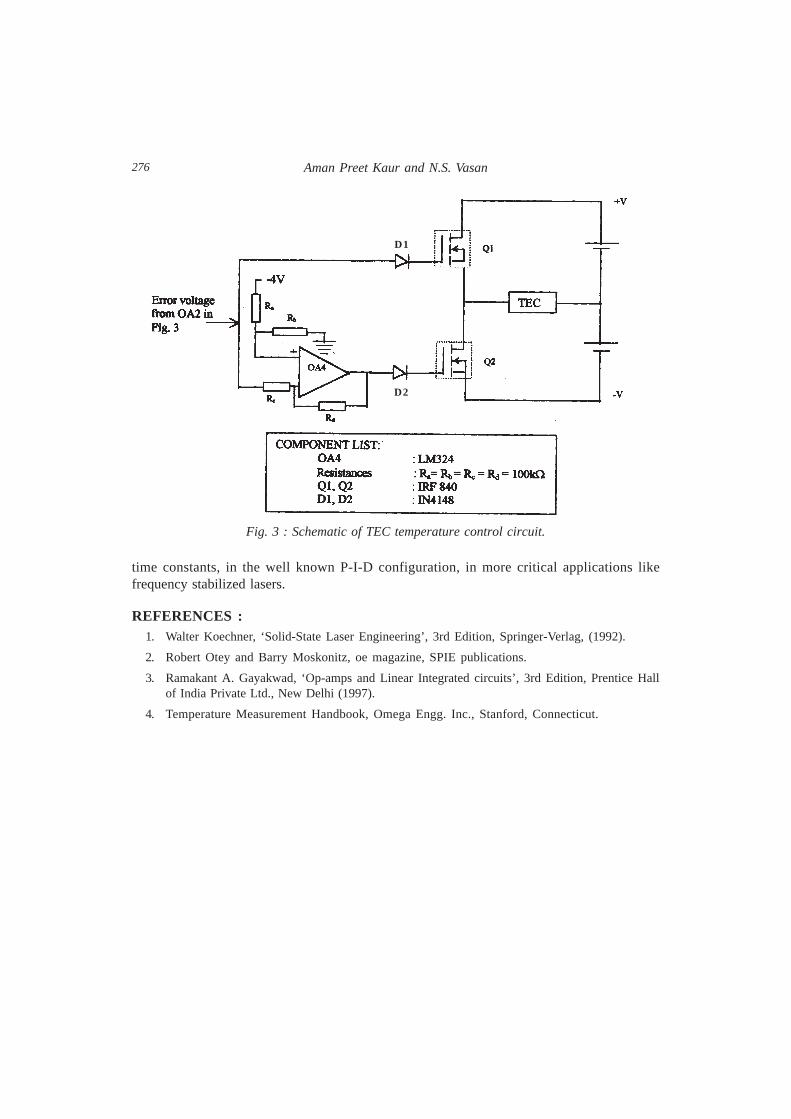
276

time constants, in the well known P-I-D configuration, in more critical applications likefrequency stabilized lasers.

REFERENCES :1. Walter Koechner, ‘Solid-State Laser Engineering’, 3rd Edition, Springer-Verlag, (1992).

2. Robert Otey and Barry Moskonitz, oe magazine, SPIE publications.

3. Ramakant A. Gayakwad, ‘Op-amps and Linear Integrated circuits’, 3rd Edition, Prentice Hallof India Private Ltd., New Delhi (1997).

4. Temperature Measurement Handbook, Omega Engg. Inc., Stanford, Connecticut.

Fig. 3 : Schematic of TEC temperature control circuit.

D1

D2

Aman Preet Kaur and N.S. Vasan

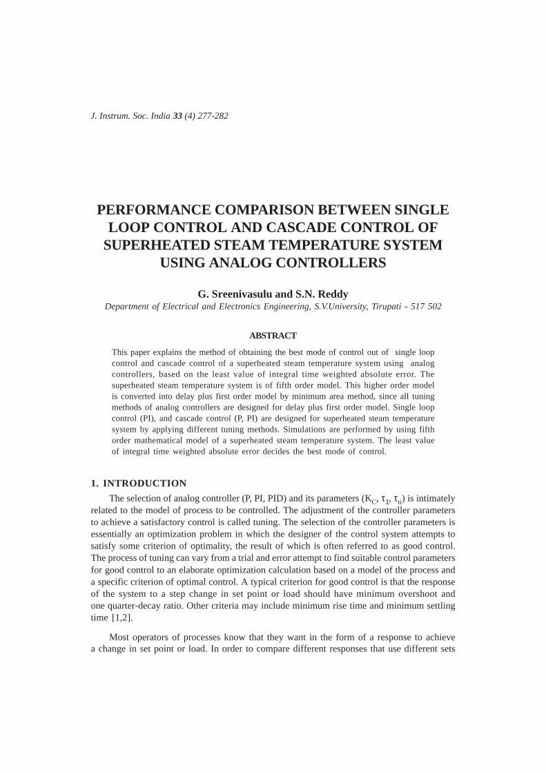
277J. Instrum. Soc. India 33 (4) 277-282

PERFORMANCE COMPARISON BETWEEN SINGLELOOP CONTROL AND CASCADE CONTROL OF

SUPERHEATED STEAM TEMPERATURE SYSTEMUSING ANALOG CONTROLLERS

G. Sreenivasulu and S.N. ReddyDepartment of Electrical and Electronics Engineering, S.V.University, Tirupati - 517 502

ABSTRACT

This paper explains the method of obtaining the best mode of control out of single loopcontrol and cascade control of a superheated steam temperature system using analogcontrollers, based on the least value of integral time weighted absolute error. Thesuperheated steam temperature system is of fifth order model. This higher order modelis converted into delay plus first order model by minimum area method, since all tuningmethods of analog controllers are designed for delay plus first order model. Single loopcontrol (PI), and cascade control (P, PI) are designed for superheated steam temperaturesystem by applying different tuning methods. Simulations are performed by using fifthorder mathematical model of a superheated steam temperature system. The least valueof integral time weighted absolute error decides the best mode of control.

1. INTRODUCTION

The selection of analog controller (P, PI, PID) and its parameters (KC, τ1, τti) is intimatelyrelated to the model of process to be controlled. The adjustment of the controller parametersto achieve a satisfactory control is called tuning. The selection of the controller parameters isessentially an optimization problem in which the designer of the control system attempts tosatisfy some criterion of optimality, the result of which is often referred to as good control.The process of tuning can vary from a trial and error attempt to find suitable control parametersfor good control to an elaborate optimization calculation based on a model of the process anda specific criterion of optimal control. A typical criterion for good control is that the responseof the system to a step change in set point or load should have minimum overshoot andone quarter-decay ratio. Other criteria may include minimum rise time and minimum settlingtime [1,2].

Most operators of processes know that they want in the form of a response to achievea change in set point or load. In order to compare different responses that use different sets

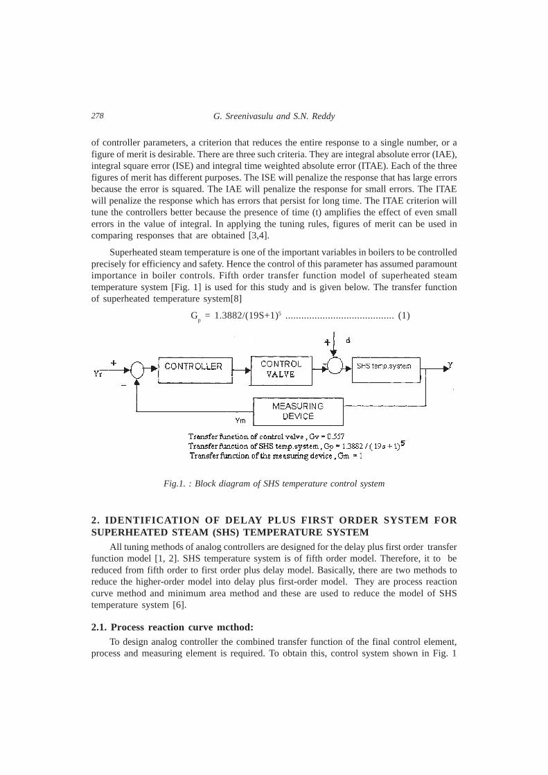
278

of controller parameters, a criterion that reduces the entire response to a single number, or afigure of merit is desirable. There are three such criteria. They are integral absolute error (IAE),integral square error (ISE) and integral time weighted absolute error (ITAE). Each of the threefigures of merit has different purposes. The ISE will penalize the response that has large errorsbecause the error is squared. The IAE will penalize the response for small errors. The ITAEwill penalize the response which has errors that persist for long time. The ITAE criterion willtune the controllers better because the presence of time (t) amplifies the effect of even smallerrors in the value of integral. In applying the tuning rules, figures of merit can be used incomparing responses that are obtained [3,4].

Superheated steam temperature is one of the important variables in boilers to be controlledprecisely for efficiency and safety. Hence the control of this parameter has assumed paramountimportance in boiler controls. Fifth order transfer function model of superheated steamtemperature system [Fig. 1] is used for this study and is given below. The transfer functionof superheated temperature system[8]

Gp = 1.3882/(19S+1)5 ......................................... (1)

2. IDENTIFICATION OF DELAY PLUS FIRST ORDER SYSTEM FORSUPERHEATED STEAM (SHS) TEMPERATURE SYSTEM

All tuning methods of analog controllers are designed for the delay plus first order transferfunction model [1, 2]. SHS temperature system is of fifth order model. Therefore, it to bereduced from fifth order to first order plus delay model. Basically, there are two methods toreduce the higher-order model into delay plus first-order model. They are process reactioncurve method and minimum area method and these are used to reduce the model of SHStemperature system [6].

2.1. Process reaction curve mcthod:To design analog controller the combined transfer function of the final control element,

process and measuring element is required. To obtain this, control system shown in Fig. 1

Fig.1. : Block diagram of SHS temperature control system

G. Sreenivasulu and S.N. Reddy

279

has been opened by disconnecting the controller from final control element. Introduce a stepinput of known magnitude at the input signal of control valve and record the response ofmeasuring element. The response Y(t) is shown in Fig. 2 (a) and is called a process reactioncurve. From the final value of the response and the given magnitude of the input signal at thecontrol valve, the steady-state gain of the combined system is calculated. Then, the slope atthe inflection point is drawn as shown in Fig. 2 (a). Since for first order system the maximumslope line starts at its origin, the delay is identified as the time at which the maximum slopeline meets the time axis (x-axis) . The time constant of the first order system is calculated forthe slope (slope=Ka/τ). Once the gain (K), the time constant(τ) and time delay (L) are known,the step response of the identified model is calculated and compared with the actual responseof the system. Thus, the delay plus first order system approximates the fifth order systemsince both of them have the same maximum slope line. Locating the inflection point and drawingthe slope at this point may be time consuming and may not be accurate. Hence minimum areamethod is used for identifying more accurate delay plus first order transfer functionmodel [4,6,12].

Fig. 2(a) : process reaction curve

Fig. 2(b) : Step response of actual system y(t) and that of delay plus first order system y(t)

Performance comparison between single loop control and cascade control

280

2.2. Minimum Area method :Process reaction curve Y(t) (normalized) and that of a first order plus time delay model

Y(t) are shown in Fig. 2 (b). The two curves are allowed to meet at two points (t1, y

1) &

(t2, y

2,). While intersection at more than two points would mean greater accuracy, a minimum

of two as shown in Fig. 2 (b) is sufficient to describe the two parameters τ and L of theSHS first order plus delay model.

The values are given by[6].

L = 1.3 t1 - 0.29 t2 .......................................... (2)

C = 0.67 (t2 - t1) . .......................................... (3)

Where t1 = time taken to reach 0.353 times of final response in sec.

t2 = time taken to reach 0.853 times of final response in sec. From the normalised stepresponse [Fig. 2 (b)] of the SI-IS Temperature system, t1 and t2 are taken at 0.353 and 0.853of the final response and are given by t1 = 74.12 sec and t2 = 138.2 sec.

Therefore, time delay, L = 1.3 t1 - 0.29 t2

= 1.3 (74.12)-0.29(138.2) L = 56.278 sec.

Time constant, τ = 0.67 (t2-t1)

= 0.67 (138.2-74.12)

τ = 42.93 sec.

From the process reaction curve shown in Fig 2 (a) the gain k=0.7717. Therefore, theidentified delay plus first order system

Ke-LS 0.7717e-56.278S

= .......................................... (4)τS+1 (42.934S+1)

3. SINGLE LOOP CONTROL OF SHS TEMPERATURE SYSTEMSingle loop control of SHS temperature system with Pl controller is shown in Fig.l. The

parameters of the PI controller are obtained by using Chien, Hrones and Reswiclc (CHR)tuning method with 20% overshoot. The formulae for parameters of Pl controller, in termsof K, L, τ of first order plus delay system based on CHR (20% overshoot) tuning method are[1, 2, 13]

Kc = 0.6τ/KL .......................................... (5)

τ1= τ .......................................... (6)

K, L, T values are obtained from the equation(4). Parameters of Pl controller are computedand are shown in Table l.

4. CASCADE CONTROL OF SHS TEMPERATURE SYSTEMCascade control of SHS temperature system with PI controller in primary loop and P

controller in secondary loop is shown in Fig. 3. The parameters of PI controller KC1

, τ1 are


281

Fig. 3 : Cascade control of SHS Temperature System

Fig. 4 : Comparison between step responses of single loop and cascade control

Performance comparison between single loop control and cascade control

282

identical to parameters of Pl controller in single loop control. The parameter of P controllerKC2 is obtained by using Ziegler - Nichols (closed loop) tuning method. The formula for KC2

based on Ziegler - Nichols (closed loop) tuning method is [5,10,11]

KC2

= 0.5 KCmax

.......................................... (7)

In simulation study, the proportional controller is cascaded with process and feedbackpath is closed. By changing the gain of proportional controller it is observed that sustainedoscillations occur at gain (Kcmax) of 3.739. The parameter K

C2, is computed using equation

(7) and parameters KC1, τ1, KC2 are shown in Table 1. [7,9,13].

RESULTS AND CONCLUSIONSUsing the mathematical model of SHS temperature system [Equation (1)] and parameters

of analog Controllers given in Table 1, responses are simulated for single loop control andcascade control in simulink of MATLAB. The responses of the SI-IS temperature system forsingle loop control and cascade control are shown in Fig. 4. l he performance of the SFIStemperature system for single loop control and cascade control are given in Table l.

Table 1. shows the performance of SHS temperature system for single loop control andcascade control to step change in set point. Cascade control of SHS temperature system havingleast value of ITAF, compared to single loop control. Hence out of single loop control andcascade control, cascade control is the best mode of control for SHS temperature system.

REFERENCESl. Astron. K.J. and T. Eiagglund, PID controllers theory design and tuning, Instrument Society

of America, 1995.2. Astrom K.J. and T.Hagglund, Automatic tuning of PID controllers, Instrument Society of

America, 1998.

3. Donald R.Coughanowr, Process systems analysis and control, 2nd edition, Mc Graw-Hill, 1991.4. George Stephanopolous, Chemical process control: An introduction to theory and practice,

PHI, New Delhi, 1999

5. I.J. Nagarth and M.Gopal Control system engineering. 2nd edition, New Age International,India, 2000.

6. M. Chidambaram, Applied process control, Allied publishers limited, India, 1998.

7. F.J. Shinskey, process control systems: Application, design & adjustment, MC Graw-Hill, 19888. The Bharath Heavy Electricals Limited, Hyderabad: Transfer function of a superheated steam

temperature system of 500MW boiler, R&D technical information sheet.

9. Astrom, K.J and T. Hagglund (1984c) “A frequency domain approach to analysis and designof simple feedback loops”, proceedings of the 23rd IEEE conference on decision and control,Las Vegas, U.S.A.

10. Gawthrop P.J. (1982), “Self Tuning PI and PID controllers”, IEEE conference on applicationsof Adoptive and Multivariable control, l-Iull.

11. Tyreus, B.D. and W.l. Luyben, “Tuning of Pl controllers for integrator/dead time processes”,Ind.eng.chem. Res., 31, 2625-2628 (1992).

12. Sunderesan, K.R. and P.R. Krishnaswamy, “Estimation of time delay, time constant parametersin time, frequency and laplace domains”, Can.J.chem.Engg., 56, 257-262 (1978).

13. B.S. Reddy, “Design of Analog controllers for superheated steam temperature system”, M.Tech thesis, S.V.University, Tirupati, India, 2002.


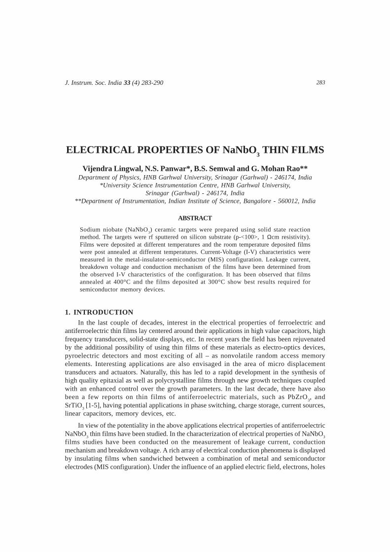
283

ELECTRICAL PROPERTIES OF NaNbO3 THIN FILMS

Vijendra Lingwal, N.S. Panwar*, B.S. Semwal and G. Mohan Rao**Department of Physics, HNB Garhwal University, Srinagar (Garhwal) - 246174, India

*University Science Instrumentation Centre, HNB Garhwal University,Srinagar (Garhwal) - 246174, India

**Department of Instrumentation, Indian Institute of Science, Bangalore - 560012, India

ABSTRACT

Sodium niobate (NaNbO3) ceramic targets were prepared using solid state reaction

method. The targets were rf sputtered on silicon substrate (p-<100>, 1 Ωcm resistivity).Films were deposited at different temperatures and the room temperature deposited filmswere post annealed at different temperatures. Current-Voltage (I-V) characteristics weremeasured in the metal-insulator-semiconductor (MIS) configuration. Leakage current,breakdown voltage and conduction mechanism of the films have been determined fromthe observed I-V characteristics of the configuration. It has been observed that filmsannealed at 400°C and the films deposited at 300°C show best results required forsemiconductor memory devices.

1. INTRODUCTIONIn the last couple of decades, interest in the electrical properties of ferroelectric and

antiferroelectric thin films lay centered around their applications in high value capacitors, highfrequency transducers, solid-state displays, etc. In recent years the field has been rejuvenatedby the additional possibility of using thin films of these materials as electro-optics devices,pyroelectric detectors and most exciting of all – as nonvolatile random access memoryelements. Interesting applications are also envisaged in the area of micro displacementtransducers and actuators. Naturally, this has led to a rapid development in the synthesis ofhigh quality epitaxial as well as polycrystalline films through new growth techniques coupledwith an enhanced control over the growth parameters. In the last decade, there have alsobeen a few reports on thin films of antiferroelectric materials, such as PbZrO

3, and

SrTiO3 [1-5], having potential applications in phase switching, charge storage, current sources,linear capacitors, memory devices, etc.

In view of the potentiality in the above applications electrical properties of antiferroelectricNaNbO3 thin films have been studied. In the characterization of electrical properties of NaNbO3

films studies have been conducted on the measurement of leakage current, conductionmechanism and breakdown voltage. A rich array of electrical conduction phenomena is displayedby insulating films when sandwiched between a combination of metal and semiconductorelectrodes (MIS configuration). Under the influence of an applied electric field, electrons, holes


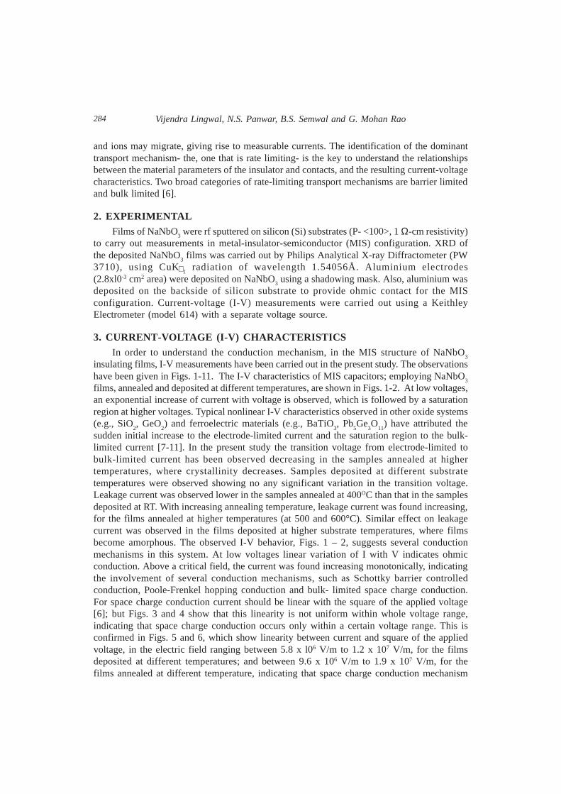
284

and ions may migrate, giving rise to measurable currents. The identification of the dominanttransport mechanism- the, one that is rate limiting- is the key to understand the relationshipsbetween the material parameters of the insulator and contacts, and the resulting current-voltagecharacteristics. Two broad categories of rate-limiting transport mechanisms are barrier limitedand bulk limited [6].

2. EXPERIMENTALFilms of NaNbO3 were rf sputtered on silicon (Si) substrates (P- <100>, 1 Ω-cm resistivity)

to carry out measurements in metal-insulator-semiconductor (MIS) configuration. XRD ofthe deposited NaNbO3 films was carried out by Philips Analytical X-ray Diffractometer (PW3710), using CuK∝ 1

radiation of wavelength 1.54056Å. Aluminium electrodes(2.8xl0-3 cm2 area) were deposited on NaNbO3 using a shadowing mask. Also, aluminium wasdeposited on the backside of silicon substrate to provide ohmic contact for the MISconfiguration. Current-voltage (I-V) measurements were carried out using a KeithleyElectrometer (model 614) with a separate voltage source.

3. CURRENT-VOLTAGE (I-V) CHARACTERISTICSIn order to understand the conduction mechanism, in the MIS structure of NaNbO3

insulating films, I-V measurements have been carried out in the present study. The observationshave been given in Figs. 1-11. The I-V characteristics of MIS capacitors; employing NaNbO3

films, annealed and deposited at different temperatures, are shown in Figs. 1-2. At low voltages,an exponential increase of current with voltage is observed, which is followed by a saturationregion at higher voltages. Typical nonlinear I-V characteristics observed in other oxide systems(e.g., SiO

2, GeO

2) and ferroelectric materials (e.g., BaTiO

3, Pb

5Ge

3O

11) have attributed the

sudden initial increase to the electrode-limited current and the saturation region to the bulk-limited current [7-11]. In the present study the transition voltage from electrode-limited tobulk-limited current has been observed decreasing in the samples annealed at highertemperatures, where crystallinity decreases. Samples deposited at different substratetemperatures were observed showing no any significant variation in the transition voltage.Leakage current was observed lower in the samples annealed at 400OC than that in the samplesdeposited at RT. With increasing annealing temperature, leakage current was found increasing,for the films annealed at higher temperatures (at 500 and 600°C). Similar effect on leakagecurrent was observed in the films deposited at higher substrate temperatures, where filmsbecome amorphous. The observed I-V behavior, Figs. 1 – 2, suggests several conductionmechanisms in this system. At low voltages linear variation of I with V indicates ohmicconduction. Above a critical field, the current was found increasing monotonically, indicatingthe involvement of several conduction mechanisms, such as Schottky barrier controlledconduction, Poole-Frenkel hopping conduction and bulk- limited space charge conduction.For space charge conduction current should be linear with the square of the applied voltage[6]; but Figs. 3 and 4 show that this linearity is not uniform within whole voltage range,indicating that space charge conduction occurs only within a certain voltage range. This isconfirmed in Figs. 5 and 6, which show linearity between current and square of the appliedvoltage, in the electric field ranging between 5.8 x l06 V/m to 1.2 x 107 V/m, for the filmsdeposited at different temperatures; and between 9.6 x 106 V/m to 1.9 x 107 V/m, for thefilms annealed at different temperature, indicating that space charge conduction mechanism

Vijendra Lingwal, N.S. Panwar, B.S. Semwal and G. Mohan Rao

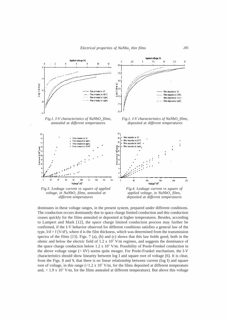
285

dominates in these voltage ranges, in the present system, prepared under different conditions.The conduction occurs dominantly due to space charge limited conduction and this conductionceases quickly for the films annealed or deposited at higher temperatures. Besides, accordingto Lampert and Mark [12], the space charge limited conduction process may further beconfirmed, if the I-V behavior observed for different conditions satisfies a general law of thetype, I/d = f (V/d2), where d is the film thickness, which was determined from the transmissionspectra of the films [13]. Figs. 7 (a), (b) and (c) shows that this law holds good, both in theohmic and below the electric field of 1.2 x 107 V/m regimes, and suggests the dominance ofthe space charge conduction below 1.2 x 107 V/m. Possibility of Poole-Frenkel conduction inthe above voltage range (< 6V) seems quite meager. For Poole-Frankel mechanism, the I-Vcharacteristics should show linearity between log I and square root of voltage [6]. It is clear,from the Figs. 8 and 9, that there is no linear relationship between current (log I) and squareroot of voltage, in this range (<1.2 x 107 V/m, for the films deposited at different temperatureand, < 1.9 x 107 V/m, for the films annealed at different temperature). But above this voltage

Fig.3. Leakage current vs square of appliedvoltage, in NaNbO3 films, annealed at

different temperatures

Fig.4. Leakage current vs square ofapplied voltage, in NaNbO3 films,deposited at different temperatures

Fig.1. I-V characteristics of NaNbO3 films,

annealed at different temperaturesFig.1. I-V characteristics of NaNbO

3 films,

deposited at different temperatures

Electrical properties of NaNbo3 thin films

286

Fig. 5. Leakage current vs square of appliedvoltage, in NaNbO

3 films, deposited at


Fig. 6. Leakage current vs square ofapplied voltage, in NaNbO

3 films,

annealed at different temperatures

Fig. 7 (a), (b) and (c). V/d2 vs I/d curvesshowing the confirmation of space charge

conduction mechanism.

Fig. 8. Log of leakage current vs squareroot of applied voltage, in NaNbO3 films,



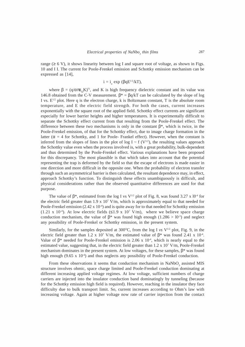
287

range (≥ 6 V), it shows linearity between log I and square root of voltage, as shown in Figs.10 and I I. The current for Poole-Frenkel emission and Schottky emission mechanism can beexpressed as [14],

i = io exp (βqE1/2/kT),

where β = (q/απεΟK)½, and K is high frequency dielectric constant and its value was146.8 obtained from the C-V measurement. β* = βq/kT can be calculated by the slope of logI vs. E1/2 plot. Here q is the electron charge, k is Boltzmann constant, T is the absolute roomtemperature, and E the electric field strength. For both the cases, current increasesexponentially with the square root of the applied field. Schottky effect currents are significantespecially for lower barrier heights and higher temperatures. It is experimentally difficult toseparate the Schottky effect current from that resulting from the Poole-Frenkel effect. Thedifference between these two mechanisms is only in the constant β*, which is twice, in thePoole-Frenkel emission, of that for the Schottky effect, due to image charge formation in thelatter (α = 4 for Schottky, and 1 for Poole- Frankel effect). However, when the constant isinferred from the slopes of lines in the plot of log I ~ f (V1/2), the resulting values approachthe Schottky value even when the process involved is, with a great probability, bulk-dependentand thus determined by the Poole-Frenkel effect. Various explanations have been proposedfor this discrepancy. The most plausible is that which takes into account that the potentialrepresenting the trap is deformed by the field so that the escape of electrons is made easier inone direction and more difficult in the opposite one. When the probability of electron transferthrough such an asymmetrical barrier is then calculated, the resultant dependence may, in effect,approach Schottky’s function. To distinguish these effects unambiguously is difficult, andphysical considerations rather than the observed quantitative differences are used for thatpurpose.

The value of β*, estimated from the log I vs V1/2 plot of Fig. 8, was found 3.27 x l0-4 forthe electric field greater than 1.9 x 107 V/m, which is approximately equal to that needed forPoole-Frenkel emission (2.42 x 10-4) and is quite away for to that needed for Schottky emission(1.21 x 10-4). At low electric fields (≤1.9 x 107 V/m), where we believe space chargeconduction mechanism, the value of β* was found high enough (1.286 > l0-3) and neglectany possibility of Poole-Frenkel or Schottky emission, in the present system.

Similarly, for the samples deposited at 300OC, from the log I vs V1/2 plot, Fig. 9, in theelectric field greater than 1.2 x 107 V/m, the estimated value of β* was found 2.41 x 10-4.Value of β* needed for Poole-Frenkel emission is 2.06 x 10-4, which is nearly equal to theestimated value, suggesting that, in the electric field greater than 1.2 x 107 V/m, Poole-Frenkelmechanism dominates in the present system. At low voltages, for these samples, β* was foundhigh enough (9.65 x 10-4) and thus neglects any possibility of Poole-Frenkel conduction.

From these observations it seems that conduction mechanism in NaNbO3 assisted MIS

structure involves ohmic, space charge limited and Poole-Frenkel conduction dominating atdifferent increasing applied voltage regimes. At low voltage, sufficient numbers of chargecarriers are injected into the insulator conduction band dominatingly by tunneling (becausefor the Schottky emission high field is required). However, reaching in the insulator they facedifficulty due to bulk transport limit. So, current increases according to Ohm’s law withincreasing voltage. Again at higher voltage now rate of carrier injection from the contact


288

Fig. 12. X-ray diffraction patterns of NaNbO3

films, deposited at different temperaturesFig. 13. X-ray diffraction patterns of NaNbO

3films, deposited at room temperature (RT) andannealed at different substrate temperatures

Fig. 11. Log of leakage current vs square root of applied voltage, in NaNbO3 films,deposited at different temperatures

Fig. 9. Log of leakage current vs square root ofapplied voltage, in NaNbO

3 films, deposited at


Fig. 10. Log of leakage current vs squareroot of applied voltage, in NaNbO

3 films,



289

(tunneling and Schottky effects) exceeds the rate at which charge can transport through thefilm. A space-charge cloud develops, that discourages further charge injection and leads tononlinear conduction effect. At higher electric fields (≥ 1.2 x 107 V/m, for the films depositedat different temperatures; and ≥ 1.9 x 107 V/m, for the films annealed at different temperatures),the trapped charge carriers jump to the conduction band leading to high current, which isPoole-Frenkel emission. In between there are indications of overlapping of both the conductionmechanisms.

Leakage current in the present samples was observed higher than the desired value formemory devices because the trends of replacing the trench and stack capacitors in DRAMs(dynamic random accessory memory) with a planar capacitor configuration prompted the needfor the development of high dielectric constant materials with low leakage current and highbreakdown strength [15, 16]. Leakage current density for the samples, deposited at roomtemperature, was calculated and was found 6.43 x 10-6 A/cm2, at 14.47 kV/cm. In the annealedsamples leakage current was found minimum (4.64 x 10-6 A/cm2, at 14.47 kV/cm) for thesamples annealed at 400°C, and it was found increasing with increasing annealing temperature.Also the leakage current was found minimum (2.5 x 10-5 A/cm2, at 14.47 kV/cm) for thesamples deposited at 270°C, and was found increasing with increasing deposition temperature.The leakage current in the present samples was found higher than that for the materialsinvestigated by others, e.g., leakage current density has been reported 2.8 x 10-6 A/cm2, at100 kV/cm, for (Ba, Sr)TiO

3, 9 x 10-8 A/cm2, at 100 kV/cm, for tantalum penta oxide (Ta

2O

5),

etc. [17, 18]. Since all the films were deposited in the argon atmosphere only, there may existoxygen vacancies, which may be the source of high conduction through insulating NaNbO

3

films. With annealing, oxygen vacancies decrease and thereby conduction decreases, in thesamples annealed at 400OC. At higher annealing temperatures (at 500 and 600OC), sodiumions might have escaped from the lattice due to their volatile nature and hence increasingconduction, in these samples. Non-stoichiometric proportion of sodium leads amorphousmaterial formation, which has also been observed in their XRD patterns, Figs.12 and 13. Inthe films, deposited at low temperatures (e.g., at RT and 270OC); conduction is not comfortablyfacilitated due to the lack of sodium vacancies. In the films deposited at higher substratetemperatures (300 and 340OC) sodium ions escape, which results high conduction and poorcrystallinity, in these films, i.e., films deposited at higher temperatures are amorphous in nature.Thus for semiconductor memory applications, where low leakage current is required, filmsannealed at 400OC give the best results among the present samples. However, for all the presentsamples, breakdown was not observed in the measured applied field range, i.e., up to 4.34 x105 V/cm. This value has been reported of the order of 105-106 V/cm, for BaTiO3 [I l].

The transport phenomena in dielectrics are not yet completely understood, that the theoryrests on models, that are too simple and that experimental results are often of dubioussignificance owing to uncertainty as to the actual conditions in the system examined. Sincethese phenomena are of great importance for electronic applications, a large amount of additionalefforts has to be devoted to them.

REFERENCESI. K. Yamakawa, S. Trolier-McKinstry, J.P. Dougherty and S.B. Krupanidhi, Appl. Phys. Lett.,

67, 2014 (1995).


290

2. I. Kanno, S. Hayashi, M. Kitagawa, R. Takayama and T. Hirao, App/. Phys. Lett., 66, 145 (1995).

3. K.K. Li, F. Wang and G.H. Haertling, J. Mater. Res., 30, 1386 (1995).

4. G.R. Bai, H.L.M. Chang, D.J. Lam and Y. Gao, Appl. Phys. Lett., 62, 1754 (1993).

5. G. Mohan Rao and S.B. Krupanidhi, J. Appl. Phys., 75, 2604 (1994).

6. S.M. Sze, ’Physics of Semiconductor Devices’, Wiley publication, New York, (2000).

7. R.V. Stuart and K.B. Wehner, J. Appl. Phys., 35, l819 (1964).

8. S.B. Krupanidhi, M. Sayer and A. Mansingh, Thin Solid Films, 113, 173 (1984).

9. J.K. Park and W.W. Granneman, Ferroelectrics, 10, 217 (1976).

10. S.B. Krupanidhi, A. Mansingh and M. Sayer, Ferroelectrics, 50, 443 (1983).

11. K. Sreenivas, Abhai Mansingh and M. Sayer, J. Appl. Phys., 62, 4475 (1987).

l2. M. Lampert and P. Mark, ’Current Injection in Solids’, Academic Press, New York, (1970).

13. S. Swanepoel, J. Phys. E: Sci. Inst., 16, 1214 (1983)

14. L. Ecketova, ‘Physics of Thin Films’, Plenum Press, New York (1977).

15. C.A. Araujo, L.D. McMillan, B.M. Melnick, J.D. Cuchiaro and J.F. Scott, Ferroelectrics, 104,241 (1990).

16. R. Moazzam, C. Hu and W.H. Shepherd, IEEE Electron Device Lett., 11, 454 (1990).

17. A. Pignolet, G. Mohan Rao, S.B. Krupanidhi, Thin Solid Films, 258, 230 (1995).

18. B. Panda, A. Dhar, G.D. Nigam, D. Bhattacharya and S.K. Ray, J. Appl. Phys., 83, 1114 (1997).


291

CONDUCTIVITY BASED PROCESS MODELLING

V. Dharmalingam and S. Sundaram*Department of Electrical and Electronics Engineering

SASTRA (Deemed University), Thanjavur-613407*Department of Chemical Engineering, Regional Engineering College, Trichy – 620 015

ABSTRACT

Cohen and Coon method has been employed in tuning of controllers for flow throughcoiled pipes of varying length. The fluid was salt solution whose conductivity wasmonitored using an online Forbes Marshall conductivity analyzer. Based on the stepresponse model parameters were established and compared with simulated values usingMATLAB. The model and the experimental values agreed within five percent.

INTRODUCTIONAll physical systems cannot be represented in their full physical intricacies and therefore

idealizing assumptions are always made for the purpose of analysis and synthesis of systems.A physical system can be modeled in a number of ways depending upon the specific problemto be dealt with and the desired accuracy. Depending on the choice of variables and the co-ordinate system, a given a greater insight into the dynamic behavior of a physical system, isselected. A commonly adopted approach for handling a new problem is to first build a simplifiedmodel, linear as for as possible, by ignoring certain nonlinearities and other physical properties,which may be present in the system and thereby get an approximate idea of the dynamicresponse. A more complex model is then built for detailed analysis1.

Various methods used for process modelling are based on key values, qualitativeevaluation, elementary pattern recognition, curve fitting and reaction curve approach. In key-values approach2 qualitative information of the signals in terms of easy to handle key-valueslike damping, overshoot and oscillation time are used. The qualitative evaluation method onthe other hand describes the signals based on qualitative terms such as ‘too low monotone’,overshoot oscillatory’ and ‘small postive’3. For elementary pattern recognition, it is assumedthat most control response patterns can be broken down and described by a basic set ofcomponent patterns4. In curve fitting approach, the time response is transferred to semi-logscale to find the process model. The general model suggested is of the form

-TdsKpe Gp(s) = ——–—––—— .......................... (1)

(T1S+1)(T2S+1)


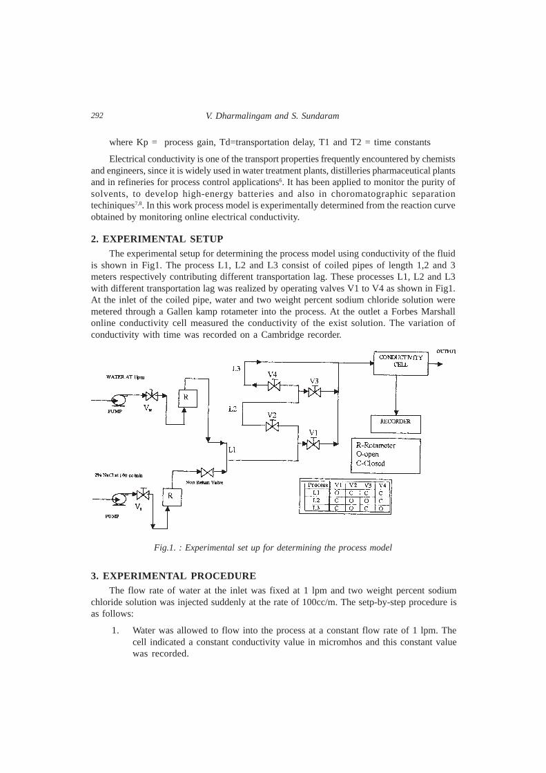
292

where Kp = process gain, Td=transportation delay, T1 and T2 = time constants

Electrical conductivity is one of the transport properties frequently encountered by chemistsand engineers, since it is widely used in water treatment plants, distilleries pharmaceutical plantsand in refineries for process control applications6. It has been applied to monitor the purity ofsolvents, to develop high-energy batteries and also in choromatographic separationtechiniques7,8. In this work process model is experimentally determined from the reaction curveobtained by monitoring online electrical conductivity.

2. EXPERIMENTAL SETUPThe experimental setup for determining the process model using conductivity of the fluid

is shown in Fig1. The process L1, L2 and L3 consist of coiled pipes of length 1,2 and 3meters respectively contributing different transportation lag. These processes L1, L2 and L3with different transportation lag was realized by operating valves V1 to V4 as shown in Fig1.At the inlet of the coiled pipe, water and two weight percent sodium chloride solution weremetered through a Gallen kamp rotameter into the process. At the outlet a Forbes Marshallonline conductivity cell measured the conductivity of the exist solution. The variation ofconductivity with time was recorded on a Cambridge recorder.

Fig.1. : Experimental set up for determining the process model

3. EXPERIMENTAL PROCEDUREThe flow rate of water at the inlet was fixed at 1 lpm and two weight percent sodium

chloride solution was injected suddenly at the rate of 100cc/m. The setp-by-step procedure isas follows:

1. Water was allowed to flow into the process at a constant flow rate of 1 lpm. Thecell indicated a constant conductivity value in micromhos and this constant valuewas recorded.

V. Dharmalingam and S. Sundaram

293

2. A two weight percent sodium chloride solution was injected at constant flow rateof 100cc/m in the inlet along with the water.

3. The conductivity of the outlet water increased slowly and reached a steady valuedepending on the pipe length. The variation in conductivity measured by the cellwas plotted by the recorded.

The variation in conductivity with respect to time for three different processes L1, L2and L3 plotted by the recorder are shown in Fig2. It is important that no disturbances otherthan the step change enter the system during the test, otherwise the transients will be corruptedby these uncontrolled disturbances and will be unsuitable for deriving a process model.

Fig.2. : Variation in conductivity with time for L1, L2 and L3

4. PROCESS MODELLINGFor many processes in the chemical industry, the process reaction curve for step input is

a sigmoidal curve. For system that produce a ‘S’ – shaped process reaction curve, a generalmodel that can be fitted to the transient is the second order with transportation lag model isshown by equation 2.

-TdsKpe

Gp(s) = ——————— .......................... (2)(T1s+1)(T2s+1)

Conductivity based process modelling

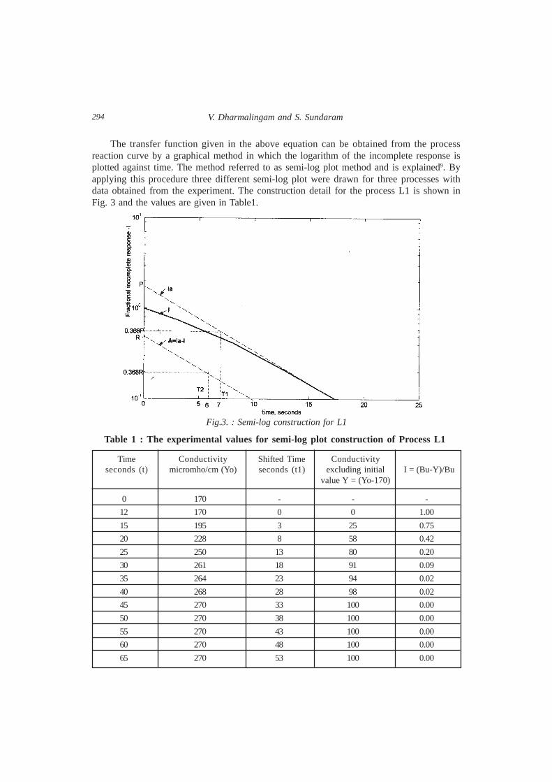
294

The transfer function given in the above equation can be obtained from the processreaction curve by a graphical method in which the logarithm of the incomplete response isplotted against time. The method referred to as semi-log plot method and is explained9. Byapplying this procedure three different semi-log plot were drawn for three processes withdata obtained from the experiment. The construction detail for the process L1 is shown inFig. 3 and the values are given in Table1.

Table 1 : The experimental values for semi-log plot construction of Process L1

Time Conductivity Shifted Time Conductivityseconds (t) micromho/cm (Yo) seconds (t1) excluding initial I = (Bu-Y)/Bu

value Y = (Yo-170)

0 170 - - -

12 170 0 0 1.00

15 195 3 25 0.75

20 228 8 58 0.42

25 250 13 80 0.20

30 261 18 91 0.09

35 264 23 94 0.02

40 268 28 98 0.02

45 270 33 100 0.00

50 270 38 100 0.00

55 270 43 100 0.00

60 270 48 100 0.00

65 270 53 100 0.00

Fig.3. : Semi-log construction for L1


295

Fig. 4. : Comparison of simulated and calculated responses with reaction curve.


296

5. RESULT AND CONCLUSIONThe variation of conductivity with time obtained from experiment for the three Processes

L1 L2 and L3 are given by the following models.

-12s 0.25e

Process L1 Gp1(S) ——————————- ......................... (3)(7s+1)(6s+1)

-23s 0.25e

Process L2 Gp2 (S) = ——————— ......................... (4)

(19s+1)(7s+1)

-32s 0.25e

Process L3 Gp3(S) = —––––––––——— ......................... (5)

(19s+1)(8s+1)

The time response for the second order transfer function having constant T1 and T2 interms of fractional incompleted ‘I’ excluding transportation lag is given by

-t/T1 -t/T2T1T2 e eI = ——— ——– ——— ......................... (6)

T1-T2 T2 T1

From equation (6) the variation in conductivity for the three different processes L1, L2and L3 were calculated. The transfer functions were also simulated using MATLAB simulationpackage. The simulated and calculated time response curves are compared with reaction curveand are shown in Fig. 4. It can be seen from that the transfer function obtained from theexperiment matches with the reaction curve. Future work on pulse, impulse and sinusoidalinput is in progress.

REFERENCES :

1. I.J. Nagrath and M. Gopal, ‘Control System Engg’, Third Edition, New Age International, NewDelhi (2001).

2. J. Lee, W. Cho, and T.F. Edgar, ‘An improved techniques for PID controller Tuning from closedloop test’, AIChE J., vol. 36, no. 12, pp. 1891-1895, 1990.

3. N.R. Sripade, D.G. Fisher and A.J. Morris, ‘AI application for process regulation and servocontrol’, IEE Proc., Part D. vol. 134, no. 4, pp. 251-59, 1987.

4. K.A. Toh and R. Devanathan, ‘Pattern-Based identification for process control applications’,IEEE Trans. Cont. Sys. Tech., vol. 4, no. 6, pp. 641-648, 1996.


297

5. A.G. Hill and W. Raksakij, ‘Process and disturbance identification by curve Fitting the closedloop response’, in Proc. Amer. Contr. Conf., pp. 2206-2209, 1989.

6. J. Schuppan, ‘Possibilities for the use of conductivity measurement in process control’, Wiss.Z. Technol. Leuna-merseburg Hochsch. ‘Carl Schorlemmer’, vol. 26, pp. 38-49, 1984.

7. J.S. Fritz, D.T. Gjerde and R.M. Becker, ‘Cation chromatography with a conductivity detector’,Anals. Chem. Vol. 52, pp. 1519-1522, 1980.

8. A. Usobiaga, A. de. Diego and J.M. Madariaga, ‘Electrical conductivity of concentratedaqueous mixture of HCl and KCl in a wide range of composition and temperatures’, J. Chem.Engg. Data, vol. 45, pp. 23-28, 2000.

9. Donald R. Coughanowr, ‘Process system analysis and control’, Second edition McGrew-HillInc, Singapore, 1991.


298

! "! # !$ ! %" %" $! " $" " !

& '" & " $ %"! (" %%$

) '!"*! "" " $ %"! $ "!"&

" " +" !" " ! " ,! "" -

.!$ / 01 0! ! 2%" !$ 2

#300! ! . " !$ "

% 2#3204 ! !$ "

.!$52+2" ! !$ "

25! " ! !$ %"

$ 2// /!

#/6 /" !708#9#0#

22 4'6 2% % 2!%"

.!$.22 . %'!: !+

.!$'!1 .!$ 2/! $!(" " ! ! $!

" / 55 6 7$! 2'9 ! $! %" .!$ 25

2" 7$! 2'9 + " " "

& !, ! " ""! !$ ": %"+" %!+ ;

% ! " !%%! +% %"

< ' $, !$ " ! ! +" $! % 08#

" + " "! $! " $" %"+" !$ " %"

2#=0! $!","!%""":&"!$>" %

!$ ! %" ! " ""! "!% !$

"" 1 %"! 0!% 2!% 4"% "%

* $ %"! , $!!, " +" " !

laser paper

Documents