Statistics and Computing manuscript No.(will be inserted by the editor)

LASSO-type estimators for Semiparametric Nonlinear Mixed-EffectsModels Estimation

Ana Arribas-Gil · Karine Bertin · Cristian Meza · Vincent Rivoirard

Received: date / Accepted: date

Abstract Parametric nonlinear mixed effects models (NLMEs)are now widely used in biometrical studies, especially inpharmacokinetics research and HIV dynamics models, dueto, among other aspects, the computational advances achievedduring the last years. However, this kind of models may notbe flexible enough for complex longitudinal data analysis.Semiparametric NLMEs (SNMMs) have been proposed asan extension of NLMEs. These models are a good compro-mise and retain nice features of both parametric and non-parametric models resulting in more flexible models thanstandard parametric NLMEs. However, SNMMs are com-plex models for which estimation still remains a challenge.Previous estimation procedures are based on a combinationof log-likelihood approximation methods for parametric es-timation and smoothing splines techniques for nonparamet-ric estimation. In this work, we propose new estimation strate-gies in SNMMs. On the one hand, we use the StochasticApproximation version of EM algorithm (SAEM) to obtainexact ML and REML estimates of the fixed effects and vari-

Ana Arribas-Gil is supported by projects MTM2010-17323 andECO2011-25706, Spain.

Karine Bertin is supported by projects FONDECYT 1090285 andECOS/CONICYT C10E03 2010, Chile.

Cristian Meza is supported by project FONDECYT 11090024, Chile.

Ana Arribas-GilDepartamento de Estadıstica, Universidad Carlos III de Madrid,Calle Madrid 126, 28903 Getafe, Spain.E-mail: ana.arribas@uc3m.es

Karine Bertin · Cristian MezaCIMFAV-Facultad de Ingenierıa, Universidad de Valparaıso,Valparaıso, Chile.E-mail: karine.bertin@uv.cl, E-mail: cristian.meza@uv.cl

Vincent RivoirardCEREMADE, CNRS-UMR 7534, Universite Paris Dauphine,Paris and INRIA Paris-Rocquencourt, Classic-team, France.E-mail: vincent.rivoirard@dauphine.fr

ance components. On the other hand, we propose a LASSO-type method to estimate the unknown nonlinear function.We derive oracle inequalities for this nonparametric estima-tor. We combine the two approaches in a general estimationprocedure that we illustrate with simulations and throughthe analysis of a real data set of price evolution in on-lineauctions.

Keywords LASSO · Nonlinear mixed-effects model ·On-line auction · SAEM algorithm · Semiparametricestimation

1 Introduction

We consider the semiparametric nonlinear mixed effects model(SNMM) as defined by Ke and Wang (2001) in which wehave n individuals and we observe:

yi j = g(xi j,φ i, f )+ εi j, εi j ∼N (0,σ2) i.i.d., (1)

i = 1, . . . ,N, j = 1, . . . ,ni,

where yi j ∈ R is the jth observation in the ith individual,xi j ∈ Rd is a known regression variable, g is a commonknown function governing within-individual behaviour andf is an unknown nonparametric function to be estimated.The random effects φ i ∈ Rp satisfy

φ i = Aiβ +η i, η i ∼N (0,Γ ) i.i.d.

where Ai ∈Mp,q are known design matrices, β ∈ Rq is theunknown vector of fixed effects and we suppose that εi j andη i are mutually independent.The parameter of the model is (θ , f ), where θ = (β ,Γ ,σ2)

belongs to a finite dimensional space whereas f belongs toan infinite dimensional space of functions denoted H .

Ke and Wang (2001) consider the most common type ofSNMM in practice, in which g is linear in f conditionally

2

on φ i,

g(xi j,φ i, f ) = a(φ i;xi j)+b(φ i;xi j) f (c(φ i;xi j)), (2)

where a, b and c are known functions which may dependon i.

Different formulations of SNMM’s have been recentlyused to model HIV dynamics (Wu and Zhang, 2002; Liuand Wu, 2007, 2008), time course microarray gene expres-sion data (Luan and Li, 2004), circadian rhythms (Wang andBrown, 1996; Wang et al, 2003), as in the following exam-ple, or to fit pharmacokinetic and pharmacodynamic models(Wang et al, 2008), among many other applications.

Example 1 The following model was proposed by Wang andBrown (1996) to fit human circadian rhythms:

yi j = µ +η1i + exp(η2i) f(

xi j−exp(η3i)

1+ exp(η3i)

)+ εi j,

εi j ∼N (0,σ2) i.i.d.

η i ∼N (0,Γ ) i.i.d.

for i = 1, . . . ,N, j = 1, . . . ,ni, where yi j is the physiologicalresponse of individual i at the jth time point xi j. This modelcan be written in the general form (1) as:

yi j = g(xi j,φ i, f )+ εi j, εi j ∼N (0,σ2) i.i.d.,

g(xi j,φ i, f ) = φ1i + exp(φ2i) f(

xi j−exp(φ3i)

1+ exp(φ3i)

)

φ i = (1,0,0)′µ +η i, η i ∼N (0,Γ ) i.i.d.

where φ i = (φ1i,φ2i,φ3i)′ and η i = (η1i,η2i,η3i)

′. In thisexample f represents the common shape of the observedcurves, and φ1i, exp(φ2i), and exp(φ3i)/(1+ exp(φ3i)) standfor the individual vertical shift, individual amplitude and in-dividual horizontal shift respectively. Here d = 1, p = 3,q = 1 and the parameter of the model is (µ,Γ ,σ2, f ). Thismodel was also used by Ke and Wang (2001) for modelingCanadian temperatures at different weather stations.

Let us introduce the following vectorial notation: yi =(yi1, . . . ,yini)

′, y = (y′1, . . . ,y′N)′, φ = (φ ′1, . . . ,φ

′N)′,

η =(η ′1, . . . ,η′N)′, gi(φ i, f )= (g(xi1,φ i, f ), . . . ,g(xini ,φ i, f ))′,

g(φ , f )= (g1(φ 1, f )′, . . . ,gN(φ n, f )′)′, A=(A′1, . . . ,A′N)′, Γ =

diag(Γ , . . . ,Γ ) and n=∑Ni=1 ni. Then, model (1) can be writ-

ten as:

y|φ ∼ N (g(φ , f ),σ2In) (3)

φ ∼ N (Aβ ,Γ )

where In is the identity matrix of dimension n, and the like-lihood of observations y is:

p(y;(θ , f )) =∫

p(y|φ ;(θ , f ))p(φ ;(θ , f ))dφ

=∫ 1(2πσ2)

n2

exp{ −1

2σ2 ‖y−g(φ , f )‖2}

× 1

(2π)N p2 |Γ |N2

exp{−1

2‖Γ−1/2

(φ −Aβ )‖2}

dφ

=1

(2π)n+N p

2 (σ2)n2 |Γ |N2

×∫

exp{−1

2

(1

σ2 ‖y−g(φ , f )‖2 +‖Γ−1/2(φ −Aβ )‖2

)}dφ ,

(4)

where ‖ · ‖ is the L2 norm. In their seminal paper, Ke andWang consider a penalized maximum likelihood approachfor the estimation of (θ , f ). That is, they propose to solve

maxθ , f{`(y;(θ , f ))−nλJ( f )} (5)

where `(y;(θ , f )) is the marginal log-likelihood, J( f ) is someroughness penalty and λ is a smoothing parameter. More-over, they assume that f belongs to some reproducing kernelHilbert space (RKHS) H = H1⊕H2, where H1 is a finitedimensional space of functions, H1 = span{ψ1, . . . ,ψM},and H2 is a RKHS itself. Since the nonlinear function f in-teracts in a complicated way with the random effects andthe integral in (4) is intractable, they replace `(y;(θ , f )) bya first-order linearization of the likelihood with respect tothe random effects. Then, they propose to estimate (θ , f ) byiterating the following two steps:

i) given an estimate of f , get estimates of θ and φ by fittingthe resultant nonlinear mixed model by linearizing thelog-likelihood (replacing ` by ˜). In practice they use theR-function nlme (Pinheiro and Bates, 2000) to solve thisstep.

ii) given an estimate of θ , θ , estimate f as the solution to

maxf∈H

{ ˜(y;(θ , f , φ))−nλJ( f )}.

Since in ii) the approximated log-likelihood involves abounded linear functional, the maximizer in H of ˜(y;(θ , f , φ))−NλJ( f ) given θ and φ belongs to a finite dimensional spaceand it is estimated as a linear combination of functions fromH1 and H2. Conceptually, the whole approach is equivalentto solving (5) not on H but on a finite-dimensional approx-imation space of H at each iteration. As it is discussed inthat article, despite of the lack of an exact solution, the splinesmoothing method provides good results and its use in thisframework is largely justified. However, the method relieson prior knowledge of the nonlinear function f and provides

3

better results when this kind of information is available.

In practice, the Ke and Wang’s method is implementedin the R package assist (Wang and Ke (2004)) and in parti-cular in the snm function which is directly related with thenlme function.As for the parametric estimation, it is important to point outsome drawbacks of the approximated methods based on lin-earization of the log-likelihood, such as the first-order lin-earization conditional estimates (FOCE) algorithm used inthe snm funtion (Wang and Ke (2004)). It has been shownthat they can produce inconsistent estimates of the fixed ef-fects, in particular when the number of measurements persubject is not large enough (Ramos and Pantula (1995); Vonesh(1996); Ge et al (2004)). Furthermore, simulation studieshave shown unexpected increases in the type I error of thelikelihood ratio and Wald tests based on these linearizationmethods (Ding and Wu (2001)). In addition, from of statis-tical point of view, the theoretical basis of this linearization-based method is weak.

Since estimation in SNMMs is an important problemand a difficult task from which many challenging aspectsarise, in this paper we propose an alternative estimation pro-cedure to tackle some of these points. On the one hand, forthe parametric step we will focus on the maximization ofthe exact likelihood. We propose to use a stochastic versionof the EM algorithm, the so-called SAEM algorithm intro-duced by Delyon et al (1999) and extended by Kuhn andLavielle (2005) for nonlinear mixed models, to estimate θwithout any approximation or linearization. This stochasticEM algorithm replaces the usual E step of EM algorithm(Dempster et al, 1977) by a simulation step and a stochasticprocedure, and converges to a local maximum of the like-lihood. The SAEM has been proved to be computationallymuch more efficient than other stochastic algorithms as forexample the classical Monte Carlo EM (MCEM) algorithm(Wei and Tanner, 1990) thanks to a recycling of the simu-lated variables from one iteration to the next (see Kuhn andLavielle (2005)). Indeed, previous attempts to perform exactML estimation in SNMMs have been discarded because ofthe computational problems related to the use of an MCEMalgorithm (see Liu and Wu (2007, 2008, 2009)). Moreoverwe use a Restricted Maximum Likelihood (REML) versionof the SAEM algorithm to correct bias estimation problemsof the variance parameters following the same strategy asMeza et al (2007).On the other hand, for the nonparametric step we will pro-pose a LASSO-type method for the estimation of f . Thepopular LASSO estimator (least absolute shrinkage and se-lection operator, Tibshirani (1996)) based on `1 penalizedleast squares, has been extended in the last years to non-parametric regression (see for instance Bickel et al (2009)).

It has been also used by Schelldorfer et al (2011) in high-dimensional linear mixed-effects models. In the nonpara-metric context, the idea is to reconstruct a sparse approxima-tion of f with linear combinations of elements of a given setof functions { f1, . . . , fM}, called dictionary. That is, we areimplicitly assuming that f can be well approximated witha small number of those functions. In practice, for the non-parametric regression problem, the dictionary can be a col-lection of basis functions from different bases (splines withfixed knots, wavelets, Fourier, etc.). The difference betweenthis approach and the smoothing splines, is that the selec-tion of the approximation function space is done automati-cally and based on data among a large collection of possi-ble spaces spanned by very different functions. This is par-ticularly important in situations in which little knowledgeabout f is available. This approach allows us to constructa good approximation of the nonparametric function whichis sparse thanks to the large dictionary. The sparsity of theapproximation gives a model more interpretable and sincefew coefficients have to be estimated, this minimizes theestimation error. The LASSO algorithm allows to use thedictionary approach to select a sparse approximation, unliketo wavelet thresholding or `0- penalization. Moreover theLASSO algorithm has a low computational cost since it isbased on a convex penalty.

We can summarize our iterative estimation procedure as:

i) given f , an estimate of f , get estimates of θ and φ byfitting the resulting NLME with the SAEM algorithm(using either ML or REML).

ii) given estimates of θ and φ , solve the resulting nonpara-metric regression problem using a LASSO-type method.

The rest of the article is organized as follows. In Sec-tion 2.1 we describe the SAEM algorithm and its REMLversion in the framework of SNMMs. In Section 3 we pro-pose a LASSO-type method for the estimation of f in theresulting nonparametric regression problem after estimationof θ and φ . Oracle inequalities and subset selection proper-ties for the proposed estimator are provided in the Supple-mentary Material. In Section 4, we describe the algorithmthat combines both procedures to perform joint estimationof (θ , f ) in the SNMM. Finally, in Section 5, we illustrateour method through a simulation study and the analysis ofprice dynamics in on-line auction data. We conclude the ar-ticle in Section 6.

2 Estimation of the finite-dimensional parameters

2.1 SAEM estimation of θ and φ

In this subsection we consider that we have an estimate off , f , obtained in the previous estimation step that does notchange during the estimation of θ . Thus, we can proceed

4

as if f was a known nonlinear function and we fall into theSAEM estimation of nonlinear mixed-effects model frame-work (see Kuhn and Lavielle (2005)). In this setting, conver-gence of the algorithm to a local maximum of the likelihoodis guaranteed. In fact, note that since the estimation of f isperformed by solving a nonparametric regression problemwith regression variables c(φ i;xi j), i= 1, . . . ,N, j = 1, . . . ,ni(see Section 3), it will depend on the estimated value of φat the precedent iteration. Then, we will note f− the currentestimated function.The complete likelihood for model (1) is:

p(y,φ ;θ) = p(y|φ ;θ)p(φ ;θ)

=1

(2π)n+N p

2 (σ2)n2 |Γ |N2

exp{−1

2

(1

σ2 ‖y−g(φ , f−)‖2

+‖Γ−1/2(φ −Aβ )‖2

)}

where n = ∑Ni=1 ni. Then, the complete log-likelihood is:

log p(y,φ ;θ) =−12{

C+n logσ2 +N log |Γ |

+1

σ2 ‖y−g(φ , f−)‖2 +N

∑i=1

(φ i−Aiβ )′Γ−1(φ i−Aiβ )

}

(6)

where C is a constant that does not depend on θ .The distribution of the complete-data model belongs to

the exponential family, that is log p(y,φ ;θ) = − Ψ(θ) +〈S(y,φ),Φ(θ)〉, where 〈·, ·〉 stands for the scalar product andS(y,φ) is the sufficient statistics. The EM algorithm in thisframework would involve the computation of E[S(y,φ)|y;θ (k)]in the E step, which in our case is intractable. The SAEM al-gorithm replaces, at each iteration, the step E by a simulationstep (S) of the missing data (φ ) and an approximation step(A). Then, iteration k of the SAEM algorithm writes:

- S step: simulate m values of the random ef-fects, φ (k+1,1), . . . ,φ (k+1,m), from the conditional lawp(·|y;θ (k)).

- A step: update sk+1 according to:

sk+1 = sk +χk

[1m

m

∑l=1

S(y,φ (k+1,l))− sk

].

- M step: update the value of θ :

θ (k+1) = argmaxθ{−Ψ(θ)+ 〈sk+1,Φ(θ)〉} (7)

where (sk)k is initialized at s0 and (χk)k is a decreasing se-quence of positive numbers which accelerates the conver-gence (Kuhn and Lavielle, 2004). The role of the sequence(χk)k is crucial in the SAEM algorithm since it performs asmoothing of the calculated likelihood values from one it-eration to another. In practice, this smoothing parameter is

defined as follows. During the first L iterations, χk = 1, andfrom iteration (L+1) the smoothing parameter starts to de-crease in order to stabilize the estimates and provide a fasterconvergence towards the true ML estimates. For example,Kuhn and Lavielle (2005) recommend to take χk =(k−L)−1

for k ≥ (L+ 1). The choices of the total number of itera-tions, K, and of L are then crucial. In order to define theseconstants, following Jank (2006) and Meza et al (2009), wemay use a graphical approach based on the likelihood diffe-rence from one iteration to the next one and monitor SAEMby estimating its progress towards θML by using the prop-erty of increasing likelihood of the EM algorithm (see formore details (Meza et al, 2009)). Then, the total number ofiterations can be fixed and the smoothing step can be de-fined. However, it is important to note that this procedureimplies to run the SAEM algorithm twice. Furthermore, asall EM-type algorithms, SAEM is sensitive to the choice ofthe initial values.

From (6), the sufficient statistics for the complete modelare given by

s1,i,k+1 = s1,i,k +χk

[1m

m

∑l=1

φ (k+1,l)i − s1,i,k

], i = 1, . . . ,N

s2,k+1 = s2,k +χk

[1m

m

∑l=1

N

∑i=1

φ (k+1,l)i φ (k+1,l)′

i − s2,k

]

s3,k+1 = s3,k +χk

[1m

m

∑l=1‖y−g(φ (k+1,l), f−)‖2− s3,k

].

Now, θ (k+1) is obtained in the maximization step as follows:

β (k+1) =

(N

∑i=1

A′iΓ(k)−1

Ai

)−1 N

∑i=1

A′iΓ(k)−1

s1,i,k+1

Γ (k+1) =1N

(s2,k+1−

N

∑i=1

Aiβ (k+1)s′1,i,k+1−N

∑i=1

s1,i,k+1

(Aiβ (k+1)

)′

+N

∑i=1

Aiβ (k+1)(Aiβ (k+1)

)′)

σ2(k+1)=

s3,k+1

n.

When the simulation step cannot be directly performed, Kuhnand Lavielle (2004) propose to combine this algorithm witha Markov Chain Monte Carlo (MCMC) procedure. Then,the simulation step becomes:

- S step: using φ (k,l), draw φ (k+1,l) with transition proba-bility Πθ (k)(·|φ (k,l)), l = 1, . . . ,m,

that is, (φ (k+1,1)), . . . ,(φ (k+1,m)) are m Markov chains withtransition kernels

(Πθ (k)

). In practice, these Markov chains

are generated using a Hastings-Metropolis algorithm (seeKuhn and Lavielle (2005) for details).With respect to the number of chains, the convergence ofthe whole algorithm to a local maximum of the likelihood is

5

granted even for m = 1. Greater values of m can acceleratethe convergence, but in practice m is always lower than 10.This is the main difference with the MCEM algorithm, inwhich very large samples of the random effects have to begenerated to obtain convergence of the algorithm.

2.2 REML estimation of variance components

It is well known that the maximum likelihood estimator ofvariance components in mixed effects models can be biaseddownwards because it does not adjust for the loss of degreesof freedom caused by the estimation of the fixed effects. Thisis also true in the context of SNMMs as Ke and Wang (2001)point out in their paper.To overcome this problem we consider restricted maximumlikelihood (REML) estimation. REML, as originally formu-lated by Patterson and Thompson (1971) in the context oflinear models, is a method that corrects this problem bymaximizing the likelihood of a set of linear functions of theobserved data that contain none of the fixed effects of themodel. But this formulation does not directly extend beyondlinear models, where in general it is not possible to constructlinear functions of the observed data that do not containany of the fixed effects. However, in the case of nonlinearmodels, other alternative formulations of REML have beenproposed. Here, we will consider the approach of Harville(1974), that consists in the maximization of the likelihoodafter integrating out the fixed effects. To perform this inte-gration we follow Foulley and Quaas (1995) and considerthe fixed effects as random with a flat prior. The combina-tion of this REML approach with the SAEM algorithm inthe context of nonlinear mixed effects models has been stud-ied recently by Meza et al (2007). The authors showed theefficiency of the method against purely ML estimation per-formed by SAEM and against REML estimation based onlikelihood approximation methods.Following these ideas we note z = (φ ,β ) the random ef-fects and θ = (Γ ,σ2) the new parameter of the model. Asin the general case, the simulation step is performed throughan MCMC procedure. Here, since we have to draw valuesfrom the joint distribution of (φ ,β )|y; θ (k), we use a Gibbsscheme, i.e., we iteratively draw values from the conditionaldistributions of φ |y,β (k); θ (k) and β |y,φ (k); θ (k). Then, weuse again a Hastings-Metropolis algorithm to obtain approx-imations of these conditional distributions.Finally, iteration k of the SAEM-REML algorithm for model(3) writes:

- S step: using z(k,l) = (φ (k,l),β (k,l)), simulatez(k+1,l) = (φ (k+1,l),β (k+1,l)), l = 1, . . . ,m with aMetropolis-within-Gibbs scheme.

- A step: update sk+1 by sk+1 = sk +

χk

[1m

m

∑l=1

S(y,z(k+1, j))− sk

], namely:

s1,k+1 = s1,k +χk

[1m

m

∑l=1

N

∑i=1

η(k+1,l)i η(k+1,l)′

i − s1,k

]

s2,k+1 = s2,k +χk

[1m

m

∑l=1‖y−g(z(k+1,l), f−)‖2− s2,k

]

where η(k+1,l)i = φ (k+1,l)

i −Aiβ (k+1,l).

- M step: update θ by θ (k+1)= argmaxθ{−Ψ(θ) +

〈sk+1,Φ(θ)〉}, namely:

Γ (k+1) =s1,k+1

Nand σ2(k+1)

=s2,k+1

n. (8)

In many situations, it is important to obtain inference onthe fixed effects in the context of REML estimation of vari-ance components. Following Meza et al (2007), estimationof fixed effects can be directly obtained as a by-product ofthe SAEM-REML algorithm via the expectation of the con-ditional distribution of the fixed effects given the observeddata, the estimate, f , of the unknown function f and theREML estimates of the variance-covariance components. Thisestimator makes sense in an Empirical Bayes framework.

3 Estimation of the function f using a LASSO-typemethod

In this part, our objective is to estimate f in the model (1)using the observations yi, j and assuming that for i = 1, . . . ,Nwe have φ i = φ i and σ2 = σ2 where the estimates φ i and σ2

have been obtained in the precedent SAEM step. Since gsatisfies (2), model (1) can be rewritten as

yi j = b(φ i;xi j) f (xi j)+ εi j, i = 1 . . . ,N, j = 1, . . . ,ni

with yi j = yi j−a(φ i;xi j) and xi j = c(φ i;xi j). Of course, sincethe φ i’s and σ2 depend on the observations, the distributionof σ−1yi j is no longer Gaussian and the εi j’s are not i.i.d. butdependent. But in the sequel, to be able to derive theoreticalresults, we still assume that

εi jiid∼N (0,σ2), (9)

where the value of σ2 is given by σ2. Simulation studies ofSection 5 show that this assumption is reasonable. However,note that (9) is true at the price of splitting the data set intotwo parts: the first part for estimating θ and φ , the secondpart for estimating f . Now, reordering the observations, it is

6

equivalent to observing (y1, . . . ,yn) with n = ∑Ni=1 ni, such

that

yi = bi f (xi)+ εi, εi ∼N (0,σ2) i.i.d. (10)

where the bi’s and the design (xi)i=1,...,n are known and de-pend on the estimators of the precedent SAEM step and theεi’s are random variables with variance σ2 estimated by σ2.Note that the notation yi, i = 1, . . . ,n, does not correspond tothe original observations in the SNMM or to any of the val-ues introduced in the previous sections, and it is used in thissection for the sake of simplicity. Without loss of generality,we suppose that bi 6= 0 for all i = 1, . . . ,n.

In the sequel, our objective is then to estimate f nonpara-metrically in model (10). A classical method would consistin decomposing f on an orthonormal basis (Fourier basis,wavelets,...) and then to use a standard nonparametric pro-cedure to estimate the coefficients of f associated with thisbasis (`0-penalization, wavelet thresholding,...). In the samespirit as Bertin et al (2011) who investigated the problemof density estimation, we wish to combine a more generaldictionary approach with an estimation procedure leading tofast algorithms. The dictionary approach consists in propos-ing estimates that are linear combinations of various typesof functions. Typically, the dictionary is built by gatheringtogether atoms of various classical orthonormal bases. Thisapproach offers two advantages. First, with a more wealthydictionary than a classical orthonormal basis, we aim at ob-taining sparse estimates leading to few estimation errors ofthe coefficients. Secondly, if the estimator is sparse enough,interesting interpretations of the results are possible by us-ing the set of the non-zero coefficients, which correspondsto the set of functions of the dictionary ”selected” by theprocedure. For instance, we can point out the frequency ofperiodic components of the signal if trigonometric functionsare selected or local peaks if some wavelets are chosen bythe algorithm. Both aspects are illustrated in the next sec-tions. `0-penalization or thresholding cannot be combinedwith a dictionary approach if we wish to obtain fast andgood algorithms. But LASSO-type estimators based on `1-penalization, leading to minimization of convex criteria, con-stitute a natural tool for the dictionary approach. Further-more, unlike ridge penalization or more generally `p-penali-zation with p > 1, `1-penalization leads to sparse solutionsfor the minimization problem, in the sense that if the tun-ing parameter is large enough some coefficients are exactlyequal to 0 (see Tibshirani (1996)).

There is now huge literature on LASSO-type procedures.From the theoretical point of view and in the specific con-text of the regression model close to (10), we mention thatLASSO procedures have already been studied by Bunea et al(2006), Bunea et al (2007a), Bunea et al (2007b), Bunea(2008), Bickel et al (2009), van de Geer (2010), and Buhlmannand van de Geer (2011) among others.

In our setting, the proposed procedure is the following.For M ∈ N∗, we consider a set of functions {ϕ1, . . . ,ϕM},called the dictionary. We denote for λ ∈ RM ,

fλ =M

∑j=1

λ jϕ j.

Our objective is to find good candidates for estimating fwhich are linear combinations of functions of the dictionary,i.e. of the form fλ . We consider, for λ ∈ RM

crit(λ ) =1n

n

∑i=1

(yi−bi fλ (xi))2 +2

M

∑j=1

rn, j|λ j|,

where rn, j = σ‖ϕ j‖n

√τ logM

n with τ > 0 and for a functionh

‖h‖2n =

1n

n

∑i=1

b2i h2(xi).

We call the LASSO estimator λ the minimizer of λ 7−→crit(λ ) for λ ∈ RM and we denote f = fλ .

The function λ 7−→ crit(λ ) is the sum of two terms: thefirst one is a goodness-of-fit criterion based on the `2-lossand the second one is a penalty term that can be viewed asthe weighted `1-norm of λ .

Before going further, let us discuss the important issueof tuning. In our context, the tuning parameter is the con-stant τ . From a theoretical point of view (see Theorem 1 inthe supplementary material), the benchmark value for τ is2. In the sequel, τ will be chosen satisfying two criteria: tobe as close as possible to this benchmark value and allowingthe stability of the SAEM algorithm. In Section 5, we willsee that sometimes we choose values of τ smaller than 2 butrelatively close of it, in particular to obtain the convergenceof the variance components estimates, which is always chal-lenging in NLME models.

Once we have chosen a value for τ satisfying these twocriteria, the numerical scheme of the nonparametric step isthe following:

- Using the estimates of the φi’s and of σ2 obtained in theprevious iteration of SAEM, compute for i= 1, . . . ,n, theobservations yi, the constants bi and the design xi.

- Evaluate the dictionary {ϕ1, . . . ,ϕM} at the design andcalculate rn, j.

- Obtain the LASSO estimates λ and fλ .

In practice, there exist many efficient algorithms to tacklethis third point, namely, the minimization on λ of crit(λ ).For the implementation of our estimation procedure we haveconsidered the approach used by Bertin et al (2011) whichconsists in using the LARS algorithm.

7

Numerical results of our procedure are presented in nextsections but we also validate our approach from a theore-tical point of view. Theoretical results are presented in thesupplementary material. We prove oracle inequalities andproperties of support for sparse functions under the mild as-sumption log(M) = o(n). Oracle inequalities ensure that theLASSO estimator of f behaves as well as the best linearcombination of functions of the dictionnary. Moreover, weobtain that if the function f is a sparse linear combinationof functions from the dictionnary, then the support of theLASSO estimator (functions of the dictionary selected in theLASSO estimator) is included in the support of the functionf . These results are generalizations of the results of Buneaet al (2006), Bunea et al (2007a), Bunea et al (2007b), van deGeer (2010) and Bunea (2008) and they are obtained undermore general assumptions on the dictionnary. In particular,in our results, the functions of the dictionary do not need tobe bounded independently of n and M, which allow us totake wavelet functions.

4 Estimation algorithm and inferences

We propose the following estimation procedure for semi-parametric estimation of (θ , f ) in model (3), combining thealgorithms described in sections 2.1 and 3:

Estimation Algorithm - ML version: at iteration k,

- Given the current estimate of θ , θ (k) =(β (k),Γ (k),σ2(k)), and m sampled values of therandom effects φ (k,l), l = 1, . . . ,m, update the estimatesof f , f (k,l), l = 1, . . . ,m, with the algorithm described inSection 3.

- Given the current estimates of f , f (k,l), l = 1, . . . ,m,sample m values of the random effects φ (k,l), l =

1, . . . ,m, and update the value of θ , θ (k+1) =(β (k+1),Γ (k+1),σ2(k+1)) with algorithm (7). (11)

Estimation Algorithm - REML version: at iteration k,

- Given the current estimate of θ , θ (k)= (Γ (k),σ2(k)),

and m sampled values of the missing data z(k,l) =(φ (k,l),β (k,l)), l = 1, . . . ,m, update the estimates of f ,f (k,l), l = 1, . . . ,m, with the algorithm described in Sec-tion 3.

- Given the current estimates of f , f (k,l), l = 1, . . . ,m,sample m values of the missing data z(k+1,l) =

(φ (k+1,l),β (k+1,l)), l = 1, . . . ,m, and update the value ofθ , θ (k+1)

= (Γ (k+1),σ2(k+1)) with algorithm (8). (12)

As it is explained in Section 2.1, for parametric estimation(SAEM or SAEM-REML algorithms alone) the number ofchains, m, can be set to 1, which still guarantees the con-vergence towards a local maximum of the log-likelihood.

Higher values of m, may accelerate the convergence of thealgorithms (but in practice, m is always lower than 10).For the global semiparametric estimation procedure, we ex-tend this idea of “parallel chains” of values to the estimationof f . Indeed, at iteration k, the estimation of f depends onthe value of the missing data, and thus, from m sampled val-ues z(k,1), . . . ,z(k,m) we obtain m estimates of f , f (k,1), . . . , f (k,m)

(see Section 3). Then, in the second step, we use each one ofthese different estimates of f in parallel to perform paramet-ric estimation (using f (k,l) to sample z(k+1,l) and replacingf− by f (k,l) in (8) for the estimation of θ ). This is in the caseof the REML version of the algorithm, but the same ideaunderlies the ML version.

Inferences on model and individual parameters, β ,Γ ,σ2

and φ , are performed as in NLMEs (see Kuhn and Lavielle(2005) and Meza et al (2007)). For inferences on the nonlin-ear function f , we propose an empirical approach based onthe fact that our algorithm automatically provides large sam-ples of estimates of f . Indeed, at each iteration of algorithms(11) and (12) we obtain m estimates of f . The last iterationsof the algorithms typically correspond to small values of χkin algorithms (7) and (8), see Section 5 for the details. Thiscan be seen as a phase in which the estimates of parametersare stabilized since we assume that convergence has beenreached. Let us note by K and L < K the total number ofiterations and the number of iterations in the “stabilizationphase” of the algorithm. Then, by considering the last L0 < Literations of the algorithm, we get a large sample of esti-mates of f : f (k,l), l = 1, . . . ,m, k = K−L0 +1, . . . ,K. Thesem×L0 estimates of f are obtained conditionally on valuesof θ which are supposed to be close to the correspondingML or REML estimates. Then, we obtain a point estimatefor f as:

f =1

m×L0

K

∑k=K−L0+1

m

∑l=1

f (k,l). (13)

We think that it will be interesting to study how to exploitthe estimates f (k,l) to obtain pointwise confidence intervalsfor f (x). An intuitive empirical pointwise (1−α)100% con-fidence interval for f (x) could be dfined as follows: f (x)− z α

2

√S2

f (x)

m×L0, f (x)+ z α

2

√S2

f (x)

m×L0

. (14)

where S2f (x)=

1m×L0−1

∑Kk=K−L0+1 ∑m

l=1( f (k,l)(x)− f (x))2

and z α2

is the 1− α2 percentile of a standard normal distri-

bution. This interval is of course not a true (1−α)100%confidence interval for f (x) but constitutes an approxima-tion of it. It provides a starting point for further research onhow function samples generated by semiparametric stochas-tic approximation algorithms, such us saem-lasso, can beused for inference.

8

5 Application to synthetic and real data

Since our procedure consists in the combination of a para-metric and a nonparametric estimation algorithm, one maybe interested in evaluating the performance of both com-ponents separately. In Section 5.1 we provide a simulationstudy to compare only the parametric versions of our methodand Ke and Wang’s procedure. In Section 5.2 we compareboth procedures in the whole semiparametric setting.

5.1 Simulation study: parametric estimation

As a first step, we want to validate through simulation ourparametric estimation strategy alone, based on the SAEMalgorithm, and to compare it, in the framework of SNMMs,to the FOCE method implemented in Ke and Wang (2001)via the nlme function. In order to be able to assess only thedifferences induced by the use of different parametric esti-mation algorithms, we will use the same nonparametric es-timation algorithm for the estimation of f , namely the pro-cedure proposed by Ke and Wang (2001). In Section 5.2, wecompare the whole versions, including nonparametric esti-mation, of both approaches.To this end, we performed the following simulation studybased in Ke and Wang (2001) where data were generatedfrom the model:

yi j = φ1i + exp(φ2i)2 f(

jN− exp(φ3i)

1+ exp(φ3i)

)+ εi j, i = 1 . . . ,N,

j = 1, . . . ,J,

where εi j ∼ N (0,σ2) and φi = (φ1i,φ2i,φ3i)′ ∼ N (µ,Γ )

with µ = (µ1,µ2,µ3)′. The nonlinear function was set to

f (t) = sin(2πt). As in the original setting, we choose a com-plex scenario with small sizes of individuals and observa-tions and with high variance values: N = J = 10, µ =(1,0,0)′,σ2 = 1 and Γ is diagonal with diag(Γ ) = (1,0.25,0.16).

These data were analyzed using two semiparametric pro-cedures: our SAEM based method combined with the non-parametric algorithm of Ke and Wang’s (called semi-SAEM)and Ke and Wang’s procedure for semiparametric models(called snm). For the SAEM algorithm, we used 80 itera-tions and the following sequence (χk): χk = 1 for 1 ≤ k ≤50 and χk = 1/(k− 50) for 51 ≤ k ≤ 80. We also consid-ered m = 5 chains in each iteration. For the nonparamet-ric estimation algorithm common to both procedures, follo-wing Ke and Wang (2001) we considered that f is periodicwith period equal to 1 and

∫ 10 f = 0, i.e. f ∈ W 0

2 (per) =W2(per) span{1} where W2(per) is the periodic Sobolevspace of order 2 in L2 and span{1} represents the set of con-stant functions. The same initial values were used for bothmethods: µ0 = (1,0,0), σ2

0 = 2 and diag(Γ0) = (γ01 ,γ

02 ,γ

03 ) =

(1,0.3,0.1).

Tables 1 and 2 summarize the performance of both meth-ods over 100 simulated data sets. For each parameter weshow the sample mean, the mean squared error (MSE(θ) =

1100

∑100i=1(θ − θi)

2), and a 95% confidence interval com-puted over the total number of simulations.

We also compared the REML estimates obtained withour method and with snm (using the REML version of nlme)for the same simulated data sets. The results are summa-rized in Tables 3 and 4. It can be seen that the mean val-ues for the REML estimates obtained with both procedureswere closer to the simulated values, especially for the pa-rameter γ1. Moreover, the individual confidence intervals ofREML estimates of this parameter, at a 95% level, includethe true value for these parameters on the contrary to theML estimates, showing that REML versions of the algo-rithms were able to correct the bias observed with ML. If wecompare our method and snm, for both procedures ML andREML, we obtained results that are similar but it seems thatour REML estimates are closer to the simulated values thanthose obtained with Ke and Wang’s method. Furthermore,we can observe that our REML version, in comparison withour ML method, allows to reduce the bias of estimation ofvariance components in a better way. For instance, in Tables2 and 4, we see that, for γ1, we reduce the bias in almost93% with our REML method whereas with Ke and Wang’sREML method this reduction is only of 27%. Finally, let uspoint out that fixed effects estimates are more accurate withour REML method than with Ke and Wang’s one. Let us re-mind that for SAEM-REML these estimates are the expec-tation of the conditional distribution of fixed effects giventhe observed data and the REML estimates of the variance-covariance parameters.

An important issue to discuss is the convergence of es-timates with this kind of iterative maximization algorithms.It is well known that approximate methods for maximumlikelihood estimation often present numerical problems andeven fail to converge in the framework of NLME estima-tion (see (Hartford and Davidian, 2000) for instance). Anadvantage of the exact likelihood method is exactly to avoidthose convergence problems as it was established by Kuhnand Lavielle (2005). In this simulation study, we have to saythat both semi-SAEM and snm achieved convergence for allthe data sets. However, we also tried to fit a nonlinear mixedeffects model to the simulated data, that is, assuming thatf was known and estimating only the fixed and random ef-fects with SAEM and nlme, and in that case the second algo-rithm failed to converge for several data sets. It seems thatin this case the combination of nlme with a nonparametricalgorithm to perform semiparametric estimation solves thenumerical problems encountered by nlme on its own. How-ever, this is not true in general as we will see in the nextsimulation study.

9

Table 1 ML procedure: Mean, MSE and 95% confidence interval of mean components.

Method µ1 µ2 µ3True Value 1 0 0

Mean semi-SAEM 1.06 0.31 0.27snm 1.05 0.26 -0.01

MSE semi-SAEM 0.12 0.16 0.10snm 0.12 0.11 0.01

95 % C.I. semi-SAEM [0.99;1.12] [0.27;0.36] [0.23;0.30]snm [0.99;1.12] [0.22;0.30] [-0.02;0.01]

Table 2 ML procedure: Mean, MSE and 95% confidence interval of variance components obtained with semi-SAEM and snm.

Method γ1 γ2 γ3 σ2

True Value 1 0.25 0.16 1Mean semi-SAEM 0.86 0.24 0.16 0.95

snm 0.89 0.19 0.14 0.99MSE semi-SAEM 0.22 0.02 0.01 0.03

snm 0.22 0.02 0.01 0.0395 % C.I. semi-SAEM [0.77;0.95] [0.21;0.27] [0.14;0.17] [0.92;0.98]

snm [0.80;0.98] [0.17;0.21] [0.13;0.16] [0.96;1.02]

Table 3 REML procedure: Mean, MSE and 95% confidence interval of mean components.

Method µ1 µ2 µ3True Value 1 0 0

Mean semi-SAEM 1.04 -0.01 -0.01snm 1.05 0.26 -0.01

MSE semi-SAEM 0.03 0.02 0.01snm 0.12 0.11 0.01

95 % C.I. semi-SAEM [1.01;1.07] [-0.03;0.02] [-0.02;0.01]snm [0.99;1.12] [0.22;0.30] [-0.02;0.01]

5.2 Simulation study: semiparametric estimation

In order to test our LASSO-based estimator we consider thesame general model of the previous section

yi j = φ1i + exp(φ2i)2 f(

jN− exp(φ3i)

1+ exp(φ3i)

)+ εi j, i = 1 . . . ,N,

j = 1, . . . ,J,

where εi j ∼ N (0,σ2) and φi = (φ1i,φ2i,φ3i)′ ∼ N (µ,Γ )

with µ = (µ1,µ2,µ3)′. Now, f (·) is supposed to be unknown

and must be estimated. It is generated as a mixture of onetrigonometric function and two Laplace densities (see Fi-gure 1).

f (t) = 0.6× sin(2πt)

+0.2×(

e−40|t−0.75|

2× ∫ 10 e−40|t−0.75|

)+0.2×

(e−40|t−0.8|

2× ∫ 10 e−40|t−0.80|

).

Data were simulated using the following parameters: N =10, J = 20, µ = (1,0,0)′, σ2 = 0.4 and Γ is diagonal withdiag(Γ ) = (0.25,0.16,0.04).The chosen function exhibits two sharp peaks that can notbe clearly distinguished by only looking at the resulting data(Figure 2). We propose this setting in order to compare theperformance of our method and snm in a situation in which

the underlying function is not smooth. Indeed, the defini-tion of Ke and Wang’s method guarantees that it will achievevery good results if the function to be estimated is well ap-proximated by combinations of spline functions. However,there might be practical situations in which assessing thesmoothness of the underlying function might not be easy.It is then interesting to investigate the performance of bothmethods in such cases.Data were analyzed using the two following semiparametricprocedures: our SAEM and LASSO based method (calledLASSO-SAEM) and Ke and Wang’s procedure for semipara-metric models, still denoted snm. For both methods we ob-tained the REML estimates of parameters.It is necessary to specify several values in order to run ouralgorithm, such as the choice of the LASSO’s tuning param-eter τ and the inputs of the SAEM algorithm (initial values,step sizes χk, number of chains in the MCMC step, numberof burn-in iterations, and total number of iterations). For thelatter, we used again 80 iterations with χk = 1 for 1≤ k≤ 50and χk = 1/(k− 50) for 51 ≤ k ≤ 80, and we consideredm = 5 chains in each iteration. The initial values, whichwere also used with snm, were: µ0 = (1,0,0), σ2

0 = 2 anddiag(Γ0) = (γ0

1 ,γ02 ,γ

03 ) = (1,0.3,0.1).

The nonparametric LASSO step has been performed withτ = 1/3. For some datasets, larger values of τ did not lead tothe stabilization of the convergence of some parameters, in

10

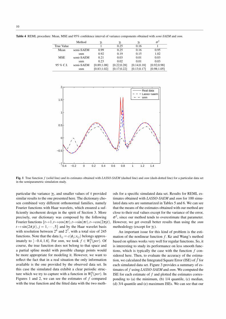
Table 4 REML procedure: Mean, MSE and 95% confidence interval of variance components obtained with semi-SAEM and snm.

Method γ1 γ2 γ3 σ2

True Value 1 0.25 0.16 1Mean semi-SAEM 0.99 0.25 0.16 0.95

snm 0.92 0.19 0.15 1.02MSE semi-SAEM 0.21 0.03 0.01 0.03

snm 0.23 0.02 0.01 0.0395 % C.I. semi-SAEM [0.89;1.08] [0.22;0.28] [0.14;0.18] [0.92;0.98]

snm [0.83;1.02] [0.17;0.22] [0.13;0.17] [0.98;1.05]

−0.4 −0.2 0 0.2 0.4 0.6 0.8 1 1.2 1.4−1

−0.5

0

0.5

1

1.5

2

Real dataLasso−saemsnm

Fig. 1 True function f (solid line) and its estimates obtained with LASSO-SAEM (dashed line) and snm (dash-dotted line) for a particular data setin the semiparametric simulation study.

particular the variance γ2, and smaller values of τ providedsimilar results to the one presented here. The dictionary cho-sen combined very different orthonormal families, namelyFourier functions with Haar wavelets, which ensured a suf-ficiently incoherent design in the spirit of Section 3. Moreprecisely, our dictionary was composed by the followingFourier functions {t 7→1, t 7→cos(πt), t 7→sin(πt), t 7→cos(2π jt),t 7→ sin(2π jt), j = 1, · · · ,5} and by the Haar wavelet basiswith resolution between 24 and 27, with a total size of 245functions. Note that the data xi j = c(φ i;xi j) belongs approx-imately to [−0.4,1.6]. For snm, we took f ∈W 0

2 (per). Ofcourse, the true function does not belong to that space anda partial spline model with possible change points wouldbe more appropriate for modeling it. However, we want toreflect the fact that in a real situation the only informationavailable is the one provided by the observed data set. Inthis case the simulated data exhibit a clear periodic struc-ture which we try to capture with a function in W 0

2 (per). InFigures 1 and 2, we can see the estimates of f comparedwith the true function and the fitted data with the two meth-

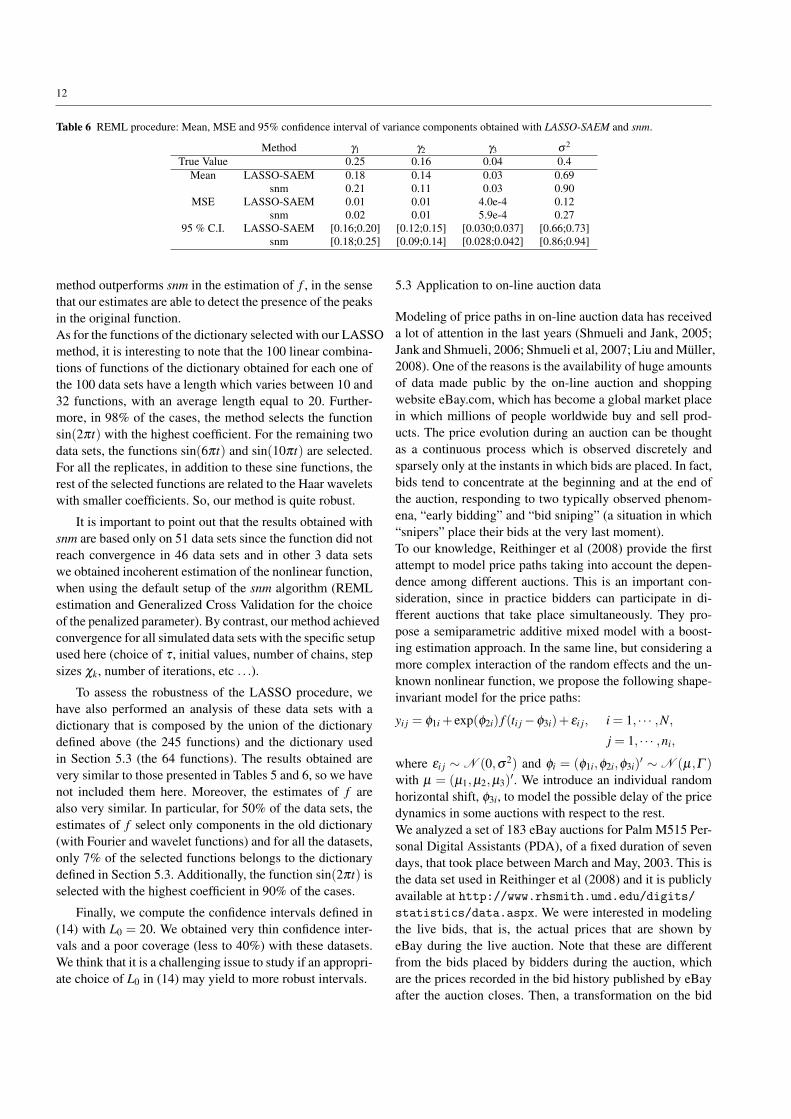
ods for a specific simulated data set. Results for REML es-timates obtained with LASSO-SAEM and snm for 100 simu-lated data sets are summarized in Tables 5 and 6. We can seethat the means of the estimates obtained with our method areclose to their real values except for the variance of the error,σ2, since our method tends to overestimate that parameter.However, we get overall better results than using the snmmethodology (except for γ1).

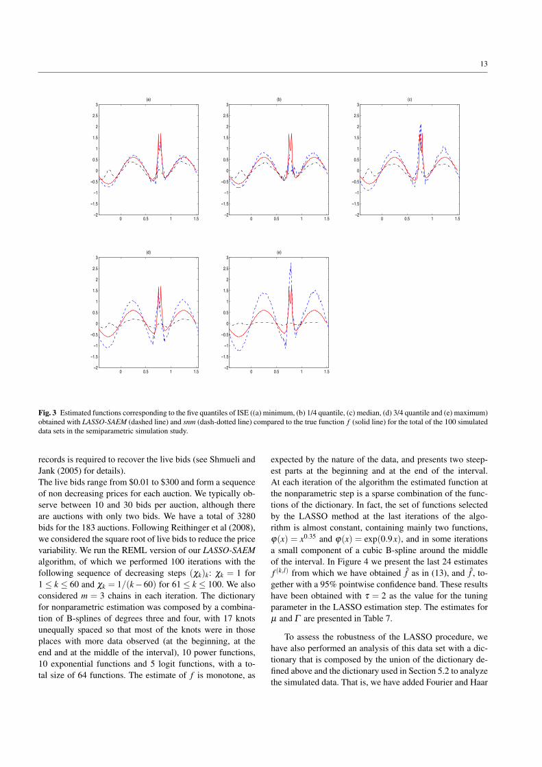
An important issue for this kind of problem is the esti-mation of the nonlinear function f . Ke and Wang’s methodbased on splines works very well for regular functions. So, itis interesting to study its performance on less smooth func-tions, which is typically the case with the function f con-sidered here. Then, to evaluate the accuracy of the estima-tion, we calculated the Integrated Square Error (ISE) of f foreach simulated data set. Figure 3 provides a summary of es-timates of f using LASSO-SAEM and snm. We computed theISE for each estimate of f and plotted the estimates corres-ponding to (a) the minimum, (b) 1/4 quantile, (c) median,(d) 3/4 quantile and (e) maximum ISEs. We can see that our

11

Covariable

Sim

ula

ted

Da

ta

−2

0

2

4

0.5 1.0 1.5 2.0

1 2

0.5 1.0 1.5 2.0

3 4

5 6 7 8

−2

0

2

4

9

0.5 1.0 1.5 2.0

10

DatasnmLasso−saem

Fig. 2 Simulated data and fitted curves obtained with LASSO-SAEM (solid line) and snm (dashed line) for a particular data set in the semiparametricsimulation study.

Table 5 REML procedure: Mean, MSE and 95% confidence interval of means components obtained with LASSO-SAEM and snm.

Method µ1 µ2 µ3True Value 1 0 0

Mean LASSO-SAEM 0.97 0.02 0.01snm 1.09 1.39 -0.01

MSE LASSO-SAEM 0.009 0.009 0.003snm 0.019 2.035 0.005

95 % C.I. LASSO-SAEM [0.949;0.984] [0.005;0.041] [-0.006;0.014]snm [1.057;1.119 ] [1.293;1.482] [-0.025;0.015]

12

Table 6 REML procedure: Mean, MSE and 95% confidence interval of variance components obtained with LASSO-SAEM and snm.

Method γ1 γ2 γ3 σ2

True Value 0.25 0.16 0.04 0.4Mean LASSO-SAEM 0.18 0.14 0.03 0.69

snm 0.21 0.11 0.03 0.90MSE LASSO-SAEM 0.01 0.01 4.0e-4 0.12

snm 0.02 0.01 5.9e-4 0.2795 % C.I. LASSO-SAEM [0.16;0.20] [0.12;0.15] [0.030;0.037] [0.66;0.73]

snm [0.18;0.25] [0.09;0.14] [0.028;0.042] [0.86;0.94]

method outperforms snm in the estimation of f , in the sensethat our estimates are able to detect the presence of the peaksin the original function.As for the functions of the dictionary selected with our LASSOmethod, it is interesting to note that the 100 linear combina-tions of functions of the dictionary obtained for each one ofthe 100 data sets have a length which varies between 10 and32 functions, with an average length equal to 20. Further-more, in 98% of the cases, the method selects the functionsin(2πt) with the highest coefficient. For the remaining twodata sets, the functions sin(6πt) and sin(10πt) are selected.For all the replicates, in addition to these sine functions, therest of the selected functions are related to the Haar waveletswith smaller coefficients. So, our method is quite robust.

It is important to point out that the results obtained withsnm are based only on 51 data sets since the function did notreach convergence in 46 data sets and in other 3 data setswe obtained incoherent estimation of the nonlinear function,when using the default setup of the snm algorithm (REMLestimation and Generalized Cross Validation for the choiceof the penalized parameter). By contrast, our method achievedconvergence for all simulated data sets with the specific setupused here (choice of τ , initial values, number of chains, stepsizes χk, number of iterations, etc . . .).

To assess the robustness of the LASSO procedure, wehave also performed an analysis of these data sets with adictionary that is composed by the union of the dictionarydefined above (the 245 functions) and the dictionary usedin Section 5.3 (the 64 functions). The results obtained arevery similar to those presented in Tables 5 and 6, so we havenot included them here. Moreover, the estimates of f arealso very similar. In particular, for 50% of the data sets, theestimates of f select only components in the old dictionary(with Fourier and wavelet functions) and for all the datasets,only 7% of the selected functions belongs to the dictionarydefined in Section 5.3. Additionally, the function sin(2πt) isselected with the highest coefficient in 90% of the cases.

Finally, we compute the confidence intervals defined in(14) with L0 = 20. We obtained very thin confidence inter-vals and a poor coverage (less to 40%) with these datasets.We think that it is a challenging issue to study if an appropri-ate choice of L0 in (14) may yield to more robust intervals.

5.3 Application to on-line auction data

Modeling of price paths in on-line auction data has receiveda lot of attention in the last years (Shmueli and Jank, 2005;Jank and Shmueli, 2006; Shmueli et al, 2007; Liu and Muller,2008). One of the reasons is the availability of huge amountsof data made public by the on-line auction and shoppingwebsite eBay.com, which has become a global market placein which millions of people worldwide buy and sell prod-ucts. The price evolution during an auction can be thoughtas a continuous process which is observed discretely andsparsely only at the instants in which bids are placed. In fact,bids tend to concentrate at the beginning and at the end ofthe auction, responding to two typically observed phenom-ena, “early bidding” and “bid sniping” (a situation in which“snipers” place their bids at the very last moment).To our knowledge, Reithinger et al (2008) provide the firstattempt to model price paths taking into account the depen-dence among different auctions. This is an important con-sideration, since in practice bidders can participate in di-fferent auctions that take place simultaneously. They pro-pose a semiparametric additive mixed model with a boost-ing estimation approach. In the same line, but considering amore complex interaction of the random effects and the un-known nonlinear function, we propose the following shape-invariant model for the price paths:

yi j = φ1i + exp(φ2i) f (ti j−φ3i)+ εi j, i = 1, · · · ,N,

j = 1, · · · ,ni,

where εi j ∼ N (0,σ2) and φi = (φ1i,φ2i,φ3i)′ ∼ N (µ,Γ )

with µ = (µ1,µ2,µ3)′. We introduce an individual random

horizontal shift, φ3i, to model the possible delay of the pricedynamics in some auctions with respect to the rest.We analyzed a set of 183 eBay auctions for Palm M515 Per-sonal Digital Assistants (PDA), of a fixed duration of sevendays, that took place between March and May, 2003. This isthe data set used in Reithinger et al (2008) and it is publiclyavailable at http://www.rhsmith.umd.edu/digits/statistics/data.aspx. We were interested in modelingthe live bids, that is, the actual prices that are shown byeBay during the live auction. Note that these are differentfrom the bids placed by bidders during the auction, whichare the prices recorded in the bid history published by eBayafter the auction closes. Then, a transformation on the bid

13

0 0.5 1 1.5−2

−1.5

−1

−0.5

0

0.5

1

1.5

2

2.5

3(a)

0 0.5 1 1.5−2

−1.5

−1

−0.5

0

0.5

1

1.5

2

2.5

3(b)

0 0.5 1 1.5−2

−1.5

−1

−0.5

0

0.5

1

1.5

2

2.5

3(c)

0 0.5 1 1.5−2

−1.5

−1

−0.5

0

0.5

1

1.5

2

2.5

3(d)

0 0.5 1 1.5−2

−1.5

−1

−0.5

0

0.5

1

1.5

2

2.5

3(e)

Fig. 3 Estimated functions corresponding to the five quantiles of ISE ((a) minimum, (b) 1/4 quantile, (c) median, (d) 3/4 quantile and (e) maximum)obtained with LASSO-SAEM (dashed line) and snm (dash-dotted line) compared to the true function f (solid line) for the total of the 100 simulateddata sets in the semiparametric simulation study.

records is required to recover the live bids (see Shmueli andJank (2005) for details).The live bids range from $0.01 to $300 and form a sequenceof non decreasing prices for each auction. We typically ob-serve between 10 and 30 bids per auction, although thereare auctions with only two bids. We have a total of 3280bids for the 183 auctions. Following Reithinger et al (2008),we considered the square root of live bids to reduce the pricevariability. We run the REML version of our LASSO-SAEMalgorithm, of which we performed 100 iterations with thefollowing sequence of decreasing steps (χk)k: χk = 1 for1 ≤ k ≤ 60 and χk = 1/(k−60) for 61 ≤ k ≤ 100. We alsoconsidered m = 3 chains in each iteration. The dictionaryfor nonparametric estimation was composed by a combina-tion of B-splines of degrees three and four, with 17 knotsunequally spaced so that most of the knots were in thoseplaces with more data observed (at the beginning, at theend and at the middle of the interval), 10 power functions,10 exponential functions and 5 logit functions, with a to-tal size of 64 functions. The estimate of f is monotone, as

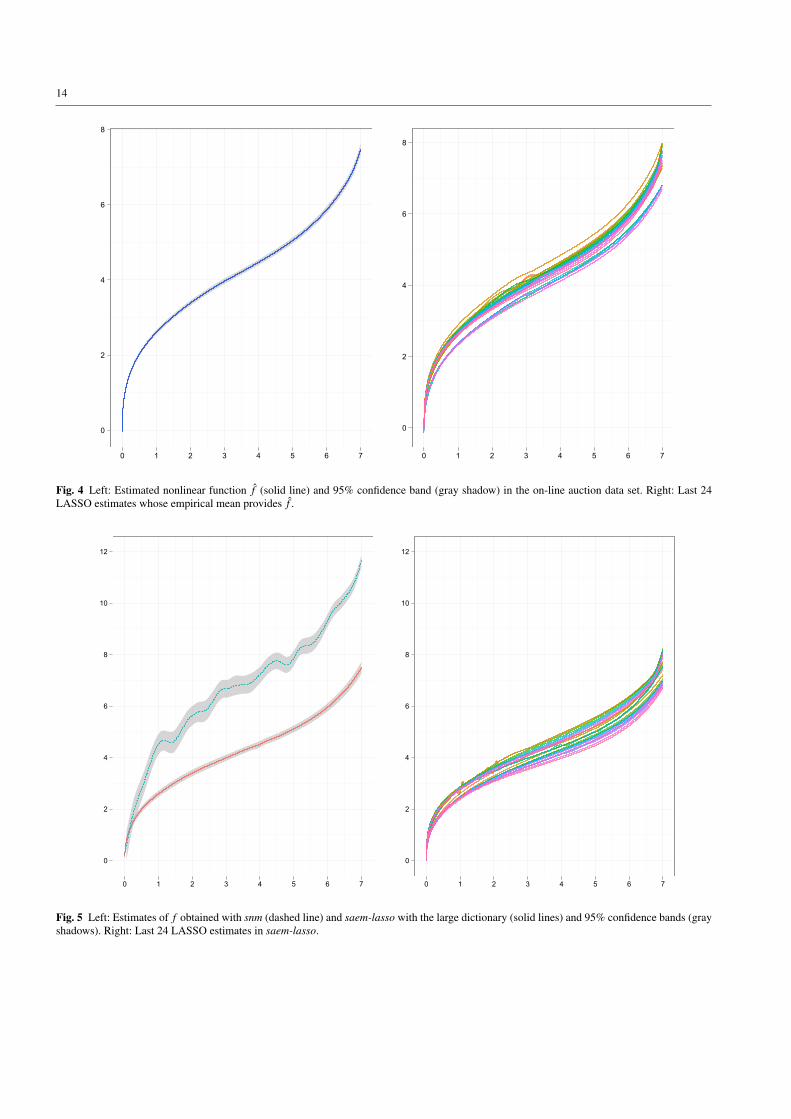
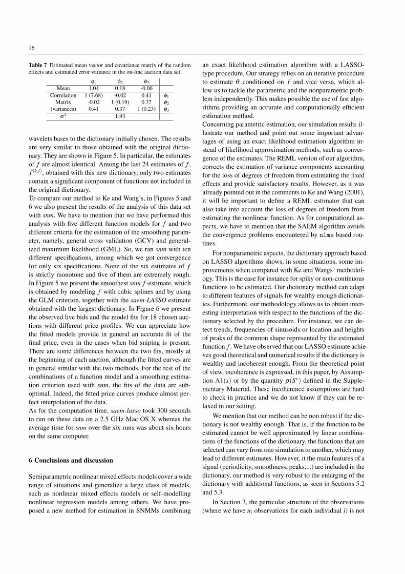
expected by the nature of the data, and presents two steep-est parts at the beginning and at the end of the interval.At each iteration of the algorithm the estimated function atthe nonparametric step is a sparse combination of the func-tions of the dictionary. In fact, the set of functions selectedby the LASSO method at the last iterations of the algo-rithm is almost constant, containing mainly two functions,ϕ(x) = x0.35 and ϕ(x) = exp(0.9x), and in some iterationsa small component of a cubic B-spline around the middleof the interval. In Figure 4 we present the last 24 estimatesf (k,l) from which we have obtained f as in (13), and f , to-gether with a 95% pointwise confidence band. These resultshave been obtained with τ = 2 as the value for the tuningparameter in the LASSO estimation step. The estimates forµ and Γ are presented in Table 7.

To assess the robustness of the LASSO procedure, wehave also performed an analysis of this data set with a dic-tionary that is composed by the union of the dictionary de-fined above and the dictionary used in Section 5.2 to analyzethe simulated data. That is, we have added Fourier and Haar

14

0

2

4

6

8

0 1 2 3 4 5 6 7

0

2

4

6

8

0 1 2 3 4 5 6 7

Fig. 4 Left: Estimated nonlinear function f (solid line) and 95% confidence band (gray shadow) in the on-line auction data set. Right: Last 24LASSO estimates whose empirical mean provides f .

0

2

4

6

8

10

12

0 1 2 3 4 5 6 7

0

2

4

6

8

10

12

0 1 2 3 4 5 6 7

Fig. 5 Left: Estimates of f obtained with snm (dashed line) and saem-lasso with the large dictionary (solid lines) and 95% confidence bands (grayshadows). Right: Last 24 LASSO estimates in saem-lasso.

15

Time

Squ

are

root

of l

ive

bids

05101520

0 2 4 6

Auction 4 Auction 9

0 2 4 6

Auction 10

Auction 13 Auction 34

05101520

Auction 4805101520

Auction 59 Auction 76 Auction 91

Auction 93 Auction 95

05101520

Auction 10005101520

Auction 102 Auction 142 Auction 160

Auction 161

0 2 4 6

Auction 170

05101520

Auction 177

Fig. 6 Observed live bids (circles) and fitted price curves for a subset of 18 auctions obtained with snm (dahsed lines) and saem-lasso (solid lines)with the large dictionary.

16

Table 7 Estimated mean vector and covariance matrix of the randomeffects and estimated error variance in the on-line auction data set.

φ1 φ2 φ3Mean 1.04 0.18 -0.06

Correlation 1 (7.68) -0.02 0.41 φ1Matrix -0.02 1 (0.19) 0.37 φ2

(variances) 0.41 0.37 1 (0.23) φ3σ2 1.93

wavelets bases to the dictionary initially chosen. The resultsare very similar to those obtained with the original dictio-nary. They are shown in Figure 5. In particular, the estimatesof f are almost identical. Among the last 24 estimates of f ,f (k,l), obtained with this new dictionary, only two estimatescontain a significant component of functions not included inthe original dictionary.To compare our method to Ke and Wang’s, in Figures 5 and6 we also present the results of the analysis of this data setwith snm. We have to mention that we have performed thisanalysis with five different function models for f and twodifferent criteria for the estimation of the smoothing param-eter, namely, general cross validation (GCV) and general-ized maximum likelihood (GML). So, we ran snm with tendifferent specifications, among which we got convergencefor only six specifications. None of the six estimates of fis strictly monotone and five of them are extremely rough.In Figure 5 we present the smoothest snm f -estimate, whichis obtained by modeling f with cubic splines and by usingthe GLM criterion, together with the saem-LASSO estimateobtained with the largest dictionary. In Figure 6 we presentthe observed live bids and the model fits for 18 chosen auc-tions with different price profiles. We can appreciate howthe fitted models provide in general an accurate fit of thefinal price, even in the cases when bid sniping is present.There are some differences between the two fits, mostly atthe beginning of each auction, although the fitted curves arein general similar with the two methods. For the rest of thecombinations of a function model and a smoothing estima-tion criterion used with snm, the fits of the data are sub-optimal. Indeed, the fitted price curves produce almost per-fect interpolation of the data.As for the computation time, saem-lasso took 300 secondsto run on these data on a 2.5 GHz Mac OS X whereas theaverage time for snm over the six runs was about six hourson the same computer.

6 Conclusions and discussion

Semiparametric nonlinear mixed effects models cover a widerange of situations and generalize a large class of models,such as nonlinear mixed effects models or self-modellingnonlinear regression models among others. We have pro-posed a new method for estimation in SNMMs combining

an exact likelihood estimation algorithm with a LASSO-type procedure. Our strategy relies on an iterative procedureto estimate θ conditioned on f and vice versa, which al-low us to tackle the parametric and the nonparametric prob-lem independently. This makes possible the use of fast algo-rithms providing an accurate and computationally efficientestimation method.Concerning parametric estimation, our simulation results il-lustrate our method and point out some important advan-tages of using an exact likelihood estimation algorithm in-stead of likelihood approximation methods, such as conver-gence of the estimates. The REML version of our algorithm,corrects the estimation of variance components accountingfor the loss of degrees of freedom from estimating the fixedeffects and provide satisfactory results. However, as it wasalready pointed out in the comments to Ke and Wang (2001),it will be important to define a REML estimator that canalso take into account the loss of degrees of freedom fromestimating the nonlinear function. As for computational as-pects, we have to mention that the SAEM algorithm avoidsthe convergence problems encountered by nlme based rou-tines.

For nonparametric aspects, the dictionary approach basedon LASSO algorithms shows, in some situations, some im-provements when compared with Ke and Wangs’ methodol-ogy. This is the case for instance for spiky or non-continuousfunctions to be estimated. Our dictionary method can adaptto different features of signals for wealthy enough dictionar-ies. Furthermore, our methodology allows us to obtain inter-esting interpretation with respect to the functions of the dic-tionary selected by the procedure. For instance, we can de-tect trends, frequencies of sinusoids or location and heightsof peaks of the common shape represented by the estimatedfunction f . We have observed that our LASSO estimate achie-ves good theoretical and numerical results if the dictionary iswealthy and incoherent enough. From the theoretical pointof view, incoherence is expressed, in this paper, by Assump-tion A1(s) or by the quantity ρ(S∗) defined in the Supple-mentary Material. These incoherence assumptions are hardto check in practice and we do not know if they can be re-laxed in our setting.

We mention that our method can be non robust if the dic-tionary is not wealthy enough. That is, if the function to beestimated cannot be well approximated by linear combina-tions of the functions of the dictionary, the functions that areselected can vary from one simulation to another, which maylead to different estimates. However, it the main features of asignal (periodicity, smoothness, peaks,...) are included in thedictionary, our method is very robust to the enlarging of thedictionary with additional functions, as seen in Sections 5.2and 5.3.

In Section 3, the particular structure of the observations(where we have ni observations for each individual i) is not

17

used for applying the standard LASSO-procedure. But a nat-ural and possible extension of this work would be to takeinto account this structure and then to apply a more sophis-ticated LASSO-type procedure inspired, for instance, by thegroup-LASSO proposed by Yuan and Lin (2006) to achievebetter results. This is a challenging research axis we wishto investigate from a theoretical and practical point of view.The LASSO is a very popular algorithm, but Hybrid Adap-tive Spline, MARS or BSML (see Sklar et al (2012)) couldalso be combined with the dictionary approach proposed inthis paper. Since results of our paper show that the dictio-nary approach seems promising, results of our paper couldbe extended by using algorithms mentioned previously fromboth theoretical and practical points of view.

Among other possible extensions of this work, a verypromising one would be the use of the nonparametric tech-niques herein described for density estimation (in the spiritof (Bertin et al, 2011)) of the random errors, assuming thatthey do not need to be normal. Indeed, the recent work ofComte and Samson (2012) deals with this problem in thecase of a linear mixed effects model. Its generalization toNLMEs or even SNMMs is a real challenge.

Acknowledgements

The authors would like to thank the anonymous AssociateEditor and two referees for valuable comments and sugges-tions.

Suppementary Material

In the supplement available on-line we provide theoreticalresults and proofs for the LASSO-type estimator of Section3.

References

Bertin K, Le Pennec E, Rivoirard V (2011) AdaptiveDantzig density estimation. Annales de l’Institut HenriPoincare 47:43–74

Bickel PJ, Ritov Y, Tsybakov AB (2009) Simultane-ous analysis of lasso and Dantzig selector. Ann Statist37(4):1705–1732

Buhlmann P, van de Geer S (2011) Statistics for high-dimensional data. Springer Series in Statistics, Springer,Heidelberg, methods, theory and applications

Bunea F (2008) Consistent selection via the Lasso for highdimensional approximating regression models. In: Push-ing the limits of contemporary statistics: contributions inhonor of Jayanta K. Ghosh, Inst. Math. Stat. Collect.,vol 3, Inst. Math. Statist., Beachwood, OH, pp 122–137

Bunea F, Tsybakov AB, Wegkamp MH (2006) Aggregationand sparsity via l1 penalized least squares. In: Learningtheory, Lecture Notes in Comput. Sci., vol 4005, Springer,Berlin, pp 379–391

Bunea F, Tsybakov A, Wegkamp M (2007a) Sparsity oracleinequalities for the Lasso. Electronic Journal of Statistics1:169–194

Bunea F, Tsybakov AB, Wegkamp MH (2007b) Aggrega-tion for Gaussian regression. The Annals of Statistics35(4):1674–1697

Comte F, Samson A (2012) Nonparametric estimationof random effects densities in linear mixed-effectsmodel, DOI oai:hal.archives-ouvertes.fr:hal-00657052,URL http://hal.archives-ouvertes.fr/hal-00657052/fr/, un-published manuscript. Available at http://hal.archives-ouvertes.fr/hal-00657052/fr/

Delyon B, Lavielle M, Moulines E (1999) Convergence ofa stochastic approximation version of the em algorithm.The Annals of Statistics 27:94–128

Dempster AP, Laird NM, Rubin DB (1977) Maximum-likelihood from incomplete data via the EM algorithm.Journal of Royal Statistical Society, Series B 39:1–38

Ding AA, Wu H (2001) Assessing antiviral potency of anti-HIV therapies in vivo by comparing viral decay rates inviral dynamic models. Biostatistics 2:13–29

Foulley JL, Quaas R (1995) Heterogeneous variances ingaussian linear mixed models. Genetics Selection Evolu-tion 27:211–228

Ge Z, Bickel P, Rice J (2004) An approximate likelihoodapproach to nonlinear mixed effects models via spline ap-proximation. Computational Statistics and Data Analysis46:747–776

van de Geer S (2010) `1-regularization in high-dimensionalstatistical models. In: Proceedings of the InternationalCongress of Mathematicians. Volume IV, HindustanBook Agency, New Delhi, pp 2351–2369

Hartford A, Davidian M (2000) Consequences of misspec-ifying assumptions in nonlinear mixed effects models.Computational Statistics & Data Analysis 34:139–164

Harville D (1974) Bayesian inference for variance compo-nents using only error contrasts. Biometrika 61:383–385

Jank W (2006) Implementing and diagnosing the stochasticapproximation em algorithm. Journal of Computational &Graphical Statistics 15(4):803–829

Jank W, Shmueli G (2006) Functional data analysis in elec-tronic commerce research. Statistical Science 21:155–166

Ke C, Wang Y (2001) Semiparametric nonlinear mixed-effects models and their applications (with discus-sion). Journal of the American Statistical Association96(456):1272–1298

Kuhn E, Lavielle M (2004) Coupling a stochastic ap-proximation version of EM with an MCMC procedure.ESAIM: P&S 8:115–131

18

Kuhn E, Lavielle M (2005) Maximum likelihood estimationin nonlinear mixed effects models. Computational Statis-tics & Data Analysis 49(4):1020–1038

Liu B, Muller HG (2008) Functional data analysis for sparseauction data. In: Jank W, Shmueli G (eds) StatisticalMethods in E-commerce research, Wiley, New York, pp269–290

Liu W, Wu L (2007) Simultaneous inference for semi-parametric nonlinear mixed-effects models with covari-ate measurement errors and missing responses. Biomet-rics 63:342–350

Liu W, Wu L (2008) A semiparametric nonlinear mixed-effects model with non-ignorable missing data and mea-surement errors for HIV viral data. Computational Statis-tics & Data Analysis 53:112–122

Liu W, Wu L (2009) Some asymptotic results for semi-parametric nonlinear mixed-effects models with incom-plete data. Journal of Statistical Planning and InferenceDoi:10.1016j.jspi.2009.06.006

Luan Y, Li H (2004) Model-based methods for identifyingperiodically expressed genes based on time course mi-croarray gene expression data. Bioinformatics 20(3):332–339

Meza C, Jaffrezic F, Foulley JL (2007) Estimation in theprobit normal model for binary outcomes using the saemalgorithm. Biometrical Journal 49(6):876–888

Meza C, Jaffrezic F, Foulley JL (2009) Reml estimation ofvariance parameters in nonlinear mixed effects modelsusing the SAEM algorithm. Computational Statistics &Data Analysis 53(4):1350–1360

Patterson HD, Thompson R (1971) Recovery of inter-blockinformation when block sizes are unequal. Biometrika58:545–554

Pinheiro J, Bates D (2000) Mixed-Effects Models in S andS-PLUS. Springer-Verlag, New York

Ramos R, Pantula S (1995) Estimation of nonlinear randomcoefficient models. Statistics & Probability Letters 24:49–56

Reithinger F, Jank W, Tutz G, Shmueli G (2008) Modellingprice paths in on-line auctions: smoothing sparse and un-evenly sampled curves by using semiparametric mixedmodels. Applied Statistics 57:127–148

Schelldorfer J, Buhlmann P, van de Geer S (2011) Esti-mation for high-dimensional linear mixed-effects modelsusing l1-penalization. Scandinavian Journal of Statistics38:197–214

Shmueli G, Jank W (2005) Visualizing online auc-tions. Journal of Computational and Graphical Statistics14:299–319

Shmueli G, Russo RP, Jank W (2007) The BARISTA: amodel for bid arrivals in online auctions. The Annals ofApplied Statistics 1:412–441

Sklar JC, Wu J, Meiring W, Wang Y (2012) Non-parametricregression with basis selection from multiple libraries.Technometrics, accepted

Tibshirani R (1996) Regression shrinkage and selection viathe Lasso. Journal of the Royal Statistical Society, SeriesB 58:267–288

Vonesh EF (1996) A note on the use of Laplace’s approx-imation for nonlinear mixed-effects models. Biometrika83:447–452

Wang Y, Brown MB (1996) A flexible model for human cir-cadian rhythms. Biometrics 52:588–596

Wang Y, Ke C (2004) Assist: A suite of s func-tions implementing spline smoothing techniques.http://wwwpstatucsbedu/faculty/yuedong/assistpdf

Wang Y, Ke C, Brown MB (2003) Shape-invariant modelingof circadian rhythms with random effects and smoothingspline anova decompositions. Biometrics 59:804–812

Wang Y, Eskridge K, Zhang S (2008) Semiparametricmixed-effects analysis of PKPD models using differentialequations. Journal of Pharmacokinetics and Pharmacody-namics 35:443–463

Wei GC, Tanner MA (1990) A Monte Carlo implementationof the EM algorithm and the poor man’s data augmenta-tion algorithm. Journal of the American Statistical Asso-ciation 85:699–704

Wu H, Zhang J (2002) The study of longterm HIV dynamicsusing semi-parametric non-linear mixed-effects models.Statistics in Medicine 21:3655–3675

Yuan M, Lin Y (2006) Model selection and estimation inregression with grouped variables. Journal of the RoyalStatistical Society, Series B 68(1):49–67

Statistics and Computing manuscript No.(will be inserted by the editor)

Supplementary Material for “LASSO-type estimators forSemiparametric Nonlinear Mixed-Effects Models Estimation”

Ana Arribas-Gil · Karine Bertin · Cristian Meza ·Vincent Rivoirard

the date of receipt and acceptance should be inserted later

1 Theoretical results for the LASSO-type estimator

1.1 Assumptions

As usual, assumptions on the dictionary are necessary to obtain oracle results for LASSO-type procedures. We refer the reader to van de Geer and Buhlmann (2009) for a good reviewof different assumptions considered in the literature for LASSO-type estimators and con-nections between them. The dictionary approach aims at extending results for orthonormalbases. Actually, our assumptions express the relaxation of the orthonormality property. Todescribe them, we introduce the following notation. For l ∈ N, we denote

νmin(l) = min|J|≤l

minλ∈RM

λJ =0

|| fλJ ||2n||λJ ||2ℓ2

and νmax(l) = max|J|≤l

maxλ∈RM

λJ =0

|| fλJ ||2n||λJ ||2ℓ2

,

where || · ||ℓ2 is the l2 norm in RM . The notation λJ means that for any k ∈ {1, . . . ,M},(λJ)k = λk if k ∈ J and (λJ)k = 0 otherwise. Previous quantities correspond to the “re-stricted” eigenvalues of the Gram matrix G = (G j, j′) with coefficients

G j, j′ =1n

n

∑i=1

b2i φ j(xi)φ j′(xi).

Assuming that νmin(l) and νmax(l) are close to 1 means that every set of columns of G withcardinality less than l behaves like an orthonormal system. We also consider the restricted

Ana Arribas-GilDepartamento de Estadıstica, Universidad Carlos III de Madrid,E-mail: ana.arribas@uc3m.es

Karine Bertin · Cristian MezaCIMFAV-Facultad de Ingenierıa, Universidad de Valparaıso,E-mail: karine.bertin@uv.cl, E-mail: cristian.meza@uv.cl

Vincent RivoirardCEREMADE, CNRS-UMR 7534, Universite Paris Dauphine,E-mail: vincent.rivoirard@dauphine.fr

2

correlations

δl,l′ = max|J|≤l|J′|≤l′

J∩J′= /0

maxλ ,λ ′∈RM

λJ =0,λ ′J′ =0

⟨ fλJ , fλ ′J′ ⟩

||λJ ||ℓ2 ||λ ′J′ ||ℓ2

,

where ⟨ f ,g⟩ = 1n ∑n

i=1 b2i f (xi)g(xi). Small values of δl,l′ means that two disjoint sets of

columns of G with cardinality less than l and l′ span nearly orthogonal spaces. We willuse the following assumption considered in Bickel et al (2009).

Assumption 1 For some integer 1 ≤ s ≤ M/2, we have

νmin(2s) > δs,2s. (A1(s))

Oracle inequalities of the Dantzig selector were established under this assumption in theparametric linear model by Candes and Tao (2007) and for density estimation by Bertin et al(2011). It was also considered by Bickel et al (2009) for nonparametric regression and forthe LASSO estimate.

Let us denote

κs =√

νmin(2s)(

1− δs,2s

νmin(2s)

)> 0, µs =

δs,2s√νmin(2s)

.

We will say that λ ∈ RM satisfies the Dantzig constraints if for all j = 1, . . . ,M∣∣∣(Gλ ) j − β j

∣∣∣≤ rn, j, (1)

where

β j =1n

n

∑i=1

biφ j(xi)Yi.

We denote D the set of λ that satisfies (1). The classical use of Karush-Kuhn-Tucker condi-tions shows that the LASSO estimator λ ∈ D , so it satisfies the Dantzig constraint. Finally,we assume in the sequel

M ≤ exp(nδ ),

for δ < 1. Therefore, if ∥φ j∥n is bounded by a constant independent of n and M, thenrn, j = o(1) and oracle inequalities established below are meaningful.

1.2 Oracle inequalities

We obtain the following oracle inequalities.

Theorem 1 Let τ > 2. With probability at least 1 − M1−τ/2, for any integer s < n/2 suchthat (A1(s)) holds, we have for any α > 0,

|| f − f ||2n ≤ infλ∈RM

infJ0⊂{1,...,M}

|J0|=s

{|| fλ − f ||2n +α

(1+

2µs

κs

)2 Λ(λ ,Jc0)

2

s+16s

(1α

+1

κ2s

)r2

n

}

(2)where

rn = supj=1,...,M

rn, j,

3

Λ(λ ,Jc0) = ||λJC

0||ℓ1 +

(||λ ||ℓ1 −||λ ||ℓ1

)+

2,

for any x ∈ R x+ := max(x,0) and || · ||ℓ1 is the l1 norm in RM .

Theorem 2 Let τ > 2. With probability at least 1 − M1−τ/2, for any integer s < n/2 suchthat (A1(s)) holds, we have for any α > 0,

|| f − f ||2n ≤ infλ∈D

infJ0⊂{1,...,M}

|J0|=s

|| fλ − f ||2n +α

(1+

2µs

κs

)2 ||λJC0||ℓ1 + ||λJC

0||ℓ1

s+32s

(1α

+1

κ2s

)r2

n

.

(3)

Similar oracle inequalities were established by Bunea et al (2006), Bunea et al (2007a),Bunea et al (2007b), or van de Geer (2010). But in these works, the functions of the dictio-nary are assumed to be bounded by a constant independent of M and n. Let us comment theright-hand side of inequalities (2) and (3) of Theorems 1 and 2. The first term is an approx-imation term which measures the closeness between f and fλ and that can vanish if f is alinear combination of the functions of the dictionary. The second term can be considered asa bias term. In both theorems, the term ||λJC

0||ℓ1 corresponds to the cost of having λ with a

support different of J0. For a given λ , this term can be minimized by choosing J0 as the setof largest coordinates of λ . Note that if the function f has a sparse expansion on the dictio-nary, that is f = fλ where λ is a vector with s non-zero coordinates, then by choosing J0 asthe set of the s non-zero coordinates, the approximation term and the term ||λJC

0||ℓ1 vanish.

In Theorem 1, the term(||λ ||ℓ1 −||λ ||ℓ1

)+

will be smaller as the ℓ1-norm of the LASSO

estimator is small and this term is equal to 0 if ||λ ||ℓ1 ≤ ||λ ||ℓ1 , which is frequently the case.In Theorem 2, given a vector λ such that fλ approximates well f , the term ||λJC

0||ℓ1 will

be small if the LASSO estimator selects the largest coordinates of λ . The last term can beviewed as a variance term corresponding to the estimation of f as linear combination of sfunctions of the dictionary (see Bertin et al (2011) for more details). Finally, the parameterα calibrates the weights given for the bias and variance terms.

The following section deals with estimation of sparse functions.

1.3 The support property of the LASSO estimate

Let τ > 2. In this section, we apply the LASSO procedure with rn, j instead of rn, j, with

rn, j = σ∥φ j∥n

√τ logM

n, τ > τ.

We assume that the regression function f can be decomposed on the dictionary: there existsλ ∗ ∈ RM such that

f =M

∑j=1

λ ∗j φ j.

We denote S∗ the support of λ ∗:

S∗ ={

j ∈ {1, . . . ,M} : λ ∗j = 0

},

4

and by s∗ the cardinal of S∗. We still consider the LASSO estimate λ and, similarly, wedenote S the support of λ :

S ={

j ∈ {1, . . . ,M} : λ j = 0}

.

One goal of this section is to show that with high probability, we have:

S ⊂ S∗.

We have the following result.

Theorem 3 We define

ρ(S∗) = maxk∈S∗

maxj =k

| < φ j,φk > |∥φ j∥n∥φk∥n

and we assume that there exists c ∈ (0,1/3) such that

s∗ρ(S∗) ≤ c.

If we have √τ +

√τ√

τ −√τ

≤ 1− c2c

,

thenP{

S ⊂ S∗}≥ 1−2M1−τ/2.

A similar result was established by Bunea (2008) in a slightly less general model. However,her result is based on strong assumptions on the dictionary, namely each function is boundedby a constant L (see Assumption (A2)(a) in Bunea (2008)). This assumption is mild whenconsidering dictionaries only based on Fourier bases. It is no longer the case when waveletsare considered and Bunea’s assumption is satisfied only in the case where L depends on Mand n on the one hand and is very large on the other hand. Since L plays a main role in thedefinition of the tuning parameters of the method, with too rough values for L, the procedurecannot achieve satisfying numerical results for moderate values of n even if asymptotictheoretical results of the procedure are good. In the setting of this paper, where we aim atproviding calibrated statistical procedures, we avoid such assumptions.

Finally, we have the following corollary.

Corollary 1 We suppose that A1(s∗) is satisfied and that there exists c ∈ (0,1/3) such that

s∗ρ(S∗) ≤ c.

If we have √τ +

√τ√

τ −√τ

≤ 1− c2c

,

then, with probability at least 1−4M1−τ/2,

|| f − f ||2n ≤ 32s∗r2n

κs∗,

wherern = sup

j=1,...,Mrn, j.

This corollary is a simple consequence of Theorem 2 with λ = λ ∗ and J0 = S∗. Takingλ = λ ∗ implies that the approximation term vanishes. Taking J0 = S∗ implies that the biasterm vanishes since the support of the LASSO estimator is included in the the support ofλ ∗. In this case, assuming that sup j ∥φ j∥n < ∞, the rate of convergence is the classical rates∗ logM

n .

5

2 The proofs

2.1 Preliminary lemma

Lemma 1 For 1 ≤ j ≤ M, we consider the event A j ={|Vj| < rn, j

}where Vj =

1n ∑n

i=1 biφ j(xi)εi.Then,

P(A j) ≥ 1−M−τ/2.

Proof of Lemma 1: We have

P(A c

j)

≤ P(√

n|Vj|/(σ∥φ j∥n) ≥ √nrn, j/(σ∥φ j∥n)

)

≤ P(|Z| ≥

√τ logM

)

≤ M−τ/2

where Z is a standard normal variable. �

2.2 Proof of Theorem 1

Let λ ∈ RM and J0 such that |J0| = s. We have

∥ fλ − f∥2n = ∥ f − f∥2

n +∥ fλ − f∥2n +

2n

n

∑i=1

b2i(

f (xi)− f (xi))(

fλ (xi)− f (xi)).

We have ∥ fλ − f∥2n = ∥ f∆ ∥2

n where ∆ = λ − λ . Moreover

A =2n

n

∑i=1

b2i(

f (xi)− f (xi))(

fλ (xi)− f (xi))

= 2M

∑j=1

(λ j − λ j)[(Gλ ) j −β j

],

where

β j =1n

n

∑i=1

b2i φ j(xi) f (xi).

Since λ satisfies the Dantzig constraint, we have with probability at least 1 − M1−τ/2, forany j ∈ {1, . . . ,M},

|(Gλ ) j −β j| ≤ |(Gλ ) j − β j|+ |β j −β j| ≤ 2rn, j

and |A| ≤ 4rn∥∆∥1. This implies that

∥ f − f ∥2n ≤ ∥ fλ − f∥2

n +4rn∥∆∥1 −∥ f∆ ∥2n.

Moreover using Lemma 1 and Proposition 1 of Bertin et al (2011) (where the norm ∥ · ∥2 isreplaced by ∥ · ∥n), we obtain that

(||∆JC

0||ℓ1 −||∆J0 ||ℓ1

)+

≤ 2||λJC0||ℓ1 +

(||λ ||ℓ1 −||λ ||ℓ1

)+

(4)

and

|| f∆ ||n ≥ κs||∆J0 ||ℓ2 − µs√|J0|

(||∆JC

0||ℓ1 −||∆J0 ||ℓ1

)+

≥ κs||∆J0 ||ℓ2 −2µs√|J0|

Λ(λ ,Jc0).

6

Note that Proposition 1 of Bertin et al (2011) is obtained using Lemma 2 and Lemma 3 ofBertin et al (2011). In our context, Lemma 2 and Lemma 3 can be proved in the same wayby replacing the norm ∥ · ∥2 by ∥ · ∥n and by considering PJ01 as the projector on the linearspace spanned by (φ j(x1), . . . ,φ j(xn)) j∈J01 .

Now following the same lines as Theorem 2 of Bertin et al (2011), replacing κJ0 by κsand µJ0 by µs, we obtain the result of the theorem.

2.3 Proof of Theorem 2

We consider λ D defined by

λ D = argminλ∈RM ||λ ||ℓ1 such that λ satisfies the Dantzig constraint (1).

Denote by f D the estimator fλ D . Following the same lines as in the proof of Theorem 1, itcan be obtained that, with probability at least 1−M1−τ/2, for any integer s < n/2 such that(A1(s)) holds, we have for any α > 0,

|| f D − f ||2n ≤ infλ∈RM

infJ0⊂{1,...,M}

|J0|=s

{|| fλ − f ||2n +α

(1+

2µs

κs

)2 Λ(λ ,Jc0)

2

s+16s

(1α

+1

κ2s

)r2

n

},

where here

Λ(λ ,Jc0) = ||λJC

0||ℓ1 +

(||λ D||ℓ1 −||λ ||ℓ1

)+

2.

If the infimum is only taken over the vectors λ that satisfy the Dantzig constraint, then, withthe same probability we have

|| f D − f ||2n ≤ infλ∈D

infJ0⊂{1,...,M}

|J0|=s

{|| fλ − f ||2n +α

(1+

2µs

κs

)2 ∥λJC0∥2

l1

s+16s

(1α

+1

κ2s

)r2

n

}.

(5)Following the same lines as the proof of Theorem 1, replacing λ by λ D, we obtain, withprobability at least 1−M1−τ/2,

∥ f − f∥2n ≤ ∥ f D − f ∥2

n +4rn∥∆∥1 −∥ f∆ ∥2n,

with ∆ = λ − λ D. Applying (4) where λ plays the role of λ and λ D the role of λ , the vector∆ satisfies (

||∆JC0||ℓ1 −||∆J0 ||ℓ1

)+

≤ 2||λJC0||ℓ1 .

Following the same lines as in the proof of Theorem 1, we obtain that for each J0 ⊂{1, . . . ,M} such that |J0| = s

|| f − f ||2n ≤

|| f D − f ||2n +α

(1+

2µs

κs

)2 ∥λJC0∥2

l1

s+16s

(1α

+1

κ2s

)r2

n

. (6)

Finally, (5) and (6) imply the theorem.

7

2.4 Proof of Theorem 3

We first state the following lemma.

Lemma 2 We have for any u ∈ RM ,

crit(λ +u)− crit(λ ) ≥∥∥∥∥∥

M

∑k=1

ukφk

∥∥∥∥∥

2

n

.

Proof of Lemma 2: Since for any λ ,

crit(λ ) =1n

n

∑i=1

(yi −bi fλ (xi))2 +2

M

∑j=1

rn, j|λ j|,

crit(λ +u)− crit(λ ) =1n

n

∑i=1

(yi −bi

M

∑k=1

λkφk(xi)−bi

M

∑k=1

ukφk(xi)

)2

+2M

∑j=1

rn, j|λ j +u j|

−1n

n

∑i=1

(yi −bi

M

∑k=1

λkφk(xi)

)2

−2M

∑j=1

rn, j|λ j|

=1n

n

∑i=1

b2i

(M

∑k=1

ukφk(xi)

)2

+2M

∑j=1

rn, j

(|λ j +u j|− |λ j|

)

−2n

n

∑i=1

(yi −bi

M

∑k=1

λkφk(xi)

)bi

M

∑k=1

ukφk(xi)

=1n

n

∑i=1

b2i

(M

∑k=1

ukφk(xi)

)2

+2M

∑j=1

rn, j

(|λ j +u j|− |λ j|

)

+2n

n

∑i=1

b2i

M

∑j=1

λ jφ j(xi)M

∑k=1

ukφk(xi)− 2n

n

∑i=1

biyi

M

∑k=1

ukφk(xi)

=1n

n

∑i=1

b2i

(M

∑k=1

ukφk(xi)

)2

+2M

∑j=1

rn, j

(|λ j +u j|− |λ j|

)

+2n

n

∑i=1

M

∑k=1

ukφk(xi)

(b2

i

M

∑j=1

λ jφ j(xi)−biyi

).

Since λ minimizes λ 7−→ crit(λ ), we have for any k,

0 =2n

n

∑i=1

φk(xi)

(b2

i

M

∑j=1

λ jφ j(xi)−biyi

)+2rn,ks(λk),

where |s(λk)| ≤ 1 and s(λk) = sign(λk) if λk = 0. So,

2n

n

∑i=1

M

∑k=1

ukφk(xi)

(b2

i

M

∑j=1

λ jφ j(xi)−biyi

)= −2

M

∑k=1

uk rn,ks(λk)

8

and

crit(λ +u)− crit(λ ) =1n

n

∑i=1

b2i

(M

∑k=1

ukφk(xi)

)2

+2M

∑j=1

rn, j

(|λ j +u j|− |λ j|

)

−2M

∑k=1

uk rn,ks(λk)

=1n

n

∑i=1

b2i

(M

∑k=1

ukφk(xi)

)2

+2M

∑j=1

rn, j

(|λ j +u j|− |λ j|−u js(λ j)

)

≥ 1n

n

∑i=1

b2i

(M

∑k=1

ukφk(xi)

)2

,

which proves the result. �

Now, still with s∗ = card(S∗), we consider for µ ∈ Rs∗

critS∗(µ) =1n

n

∑i=1

(yi −bi ∑

j∈S∗µ jφ j(xi)

)2

+2 ∑j∈S∗

rn, j|µ j|,

andµ = arg min

µ∈Rs∗critS∗(µ).

Then we set

S =∩

j/∈S∗

{∣∣∣∣∣1n

n

∑i=1

yibiφ j(xi)− ∑k∈S∗

µk < φ j,φk >

∣∣∣∣∣< rn, j

}

and we state the following lemma.

Lemma 3 On the set S , the non-zero coordinates of λ are included into S∗.

Proof of Lemma 3: Recall that λ is a minimizer of λ 7−→ crit(λ ). Using standard convexanalysis arguments, this is equivalent to say that for any 1 ≤ j ≤ M,

1n ∑n

i=1 yibiφ j(xi)−∑Mk=1 λk < φ j,φk > = rn, jsign(λ j) if λ j = 0,

∣∣∣ 1n ∑n

i=1 yibiφ j(xi)−∑Mk=1 λk < φ j,φk >

∣∣∣ ≤ rn, j if λ j = 0.

Similarly, on S , we have

1n ∑n

i=1 yibiφ j(xi)−∑k∈S∗ µk < φ j,φk > = rn, jsign(µ j) if j ∈ S∗ and µ j = 0,

∣∣ 1n ∑n

i=1 yibiφ j(xi)−∑k∈S∗ µk < φ j,φk >∣∣ ≤ rn, j if j ∈ S∗ and µ j = 0,

∣∣ 1n ∑n

i=1 yibiφ j(xi)−∑k∈S∗ µk < φ j,φk >∣∣ < rn, j if j /∈ S∗.

So, on S , the vector µ such µ j = µ j if j ∈ S∗ and µ j = 0 if j /∈ S∗ is also a minimizer ofλ 7−→ crit(λ ). Using Lemma 2, we have for any 1 ≤ i ≤ n:

M

∑k=1

(λk − µk)φk(xi) = 0.

9

So, for j /∈ S∗, ∣∣∣∣∣1n

n

∑i=1

yibiφ j(xi)−M

∑k=1

λk < φ j,φk >

∣∣∣∣∣< rn, j.

Therefore, on S , the non-zero coordinates of λ are included into S∗. �

Lemma 3 shows that we just need to prove that

P{S } ≥ 1−2M1−τ/2

P{S c} ≤ ∑j/∈S∗

P

{∣∣∣∣∣1n

n

∑i=1

yibiφ j(xi)− ∑k∈S∗

µk < φ j,φk >

∣∣∣∣∣≥ rn, j

}

≤ A+B,

with

A = ∑j/∈S∗

P

{∣∣∣∣∣1n

n

∑i=1

[yibiφ j(xi)−E(yibiφ j(xi))]

∣∣∣∣∣≥ rn, j

}

= ∑j/∈S∗

P

{∣∣∣∣∣1n

n

∑i=1

εibiφ j(xi)

∣∣∣∣∣≥ rn, j

}

= ∑j/∈S∗

P{∣∣Vj

∣∣≥ rn, j}

(see Lemma 1) and

B = P

∪

j/∈S∗

{∣∣∣∣∣1n

n

∑i=1

E(yibiφ j(xi))− ∑k∈S∗

µk < φ j,φk >

∣∣∣∣∣≥ rn, j − rn, j

}

= P

∪

j/∈S∗

{∣∣∣∣∣< φ j, fλ ∗ > − ∑k∈S∗

µk < φ j,φk >

∣∣∣∣∣≥ rn, j − rn, j

}

= P

∪

j/∈S∗

{∣∣∣∣∣∑k∈S∗(λ ∗

k − µk) < φ j,φk >

∣∣∣∣∣≥ rn, j − rn, j

}

≤ P

∪

j/∈S∗

{ρ(S∗)∥φ j∥n ∑

k∈S∗|λ ∗

k − µk|∥φk∥n ≥ rn, j − rn, j

}

since

ρ(S∗) = maxk∈S∗

maxj =k

| < φ j,φk > |∥φ j∥n∥φk∥n

.

Using notation of Lemma 3, we have:

∥ fλ ∗ − fµ∥2n = ∥ ∑

k∈S∗(λ ∗

k − µk)φk∥2n

= ∑k∈S∗

(λ ∗k − µk)

2∥φk∥2n + ∑

k∈S∗∑

j∈S∗, j =k(λ ∗

k − µk)(λ ∗j − µ j) < φ j,φk >,

10

and

∑k∈S∗

(λ ∗k − µk)

2∥φk∥2n ≤ ∥ fλ ∗ − fµ∥2

n +ρ(S∗) ∑k∈S∗

∑j∈S∗, j =k

|λ ∗k − µk|∥φk∥n ×|λ ∗

j − µ j|∥φ j∥n

≤ ∥ fλ ∗ − fµ∥2n +ρ(S∗)

(∑

k∈S∗|λ ∗

k − µk|∥φk∥n

)2

.

Finally,

(∑

k∈S∗|λ ∗

k − µk|∥φk∥n

)2

≤ s∗ ∑k∈S∗

(λ ∗k − µk)

2∥φk∥2n

≤ s∗

∥ fλ ∗ − fµ∥2

n +ρ(S∗)

(∑

k∈S∗|λ ∗

k − µk|∥φk∥n

)2 ,

which shows that

(∑

k∈S∗|λ ∗

k − µk|∥φk∥n

)2

≤ s∗

1−ρ(S∗)s∗ ∥ fλ ∗ − fµ∥2n.

Now,

1n

n

∑i=1

(yi −bi ∑

j∈S∗µ jφ j(xi)

)2

+2 ∑j∈S∗

rn, j|µ j| ≤

1n

n

∑i=1

(yi −bi ∑

j∈S∗λ ∗

j φ j(xi)

)2

+2 ∑j∈S∗

rn, j|λ ∗j |.

So,

∥ ∑j∈S∗

µ jφ j∥2n − 2

n

n

∑i=1

biyi ∑j∈S∗

µ jφ j(xi)+2 ∑j∈S∗

rn, j|µ j| ≤

∥ ∑j∈S∗

λ ∗j φ j∥2

n − 2n

n

∑i=1

biyi ∑j∈S∗

λ ∗j φ j(xi)+2 ∑

j∈S∗rn, j|λ ∗

j |,

and using previous notation,

∥ fµ∥2n − 2

n

n

∑i=1

biyi ∑j∈S∗

µ jφ j(xi)+2 ∑j∈S∗

rn, j|µ j| ≤

∥ fλ ∗∥2n − 2

n

n

∑i=1

biyi ∑j∈S∗

λ ∗j φ j(xi)+2 ∑

j∈S∗rn, j|λ ∗

j |.

11

Therefore,

∥ fλ ∗ − fµ∥2n = ∥ fµ∥2

n +∥ fλ ∗∥2n −2 < fµ , fλ ∗ >

≤ 2∥ fλ ∗∥2n −2 < fµ , fλ ∗ > +

2n

n

∑i=1

biyi ∑j∈S∗

(µ j −λ ∗j )φ j(xi)+2 ∑

j∈S∗rn, j(|λ ∗

j |− |µ j|)

=2n

n

∑i=1

biyi( fµ(xi)− fλ ∗(xi))− 2n

n

∑i=1

b2i fλ ∗(xi)( fµ(xi)− fλ ∗(xi))

+2 ∑j∈S∗

rn, j(|λ ∗j |− |µ j|)

=2n

n

∑i=1

bi(yi −E(yi))( fµ(xi)− fλ ∗(xi))+2 ∑j∈S∗

rn, j(|λ ∗j |− |µ j|)

=2n

n

∑i=1

biεi( fµ(xi)− fλ ∗(xi))+2 ∑j∈S∗

rn, j(|λ ∗j |− |µ j|)

= 2M

∑j=1

Vj(µ j −λ ∗j )+2 ∑

j∈S∗rn, j(|λ ∗

j |− |µ j|).

Now let us assume that for any j ∈ S∗, Vj < rn, j. Then,

∥ fλ ∗ − fµ∥2n < 2 ∑

j∈S∗(rn, j + rn, j)|µ j −λ ∗

j |

< 2σ√

logMn

(√

τ +√

τ) ∑j∈S∗

∥φ j∥n|µ j −λ ∗j |.

So,

∑k∈S∗

|λ ∗k − µk|∥φk∥n < 2σ

√logM

n(√

τ +√

τ)s∗

1−ρ(S∗)s∗

and for any j /∈ S∗,

ρ(S∗)∥φ j∥n ∑k∈S∗

|λ ∗k − µk|∥φk∥n < 2σ

√logM

n∥φ j∥n(

√τ +

√τ)

ρ(S∗)s∗

1−ρ(S∗)s∗

<2σc(

√τ +

√τ)

1− c

√logM

n∥φ j∥n

< (√

τ −√

τ)σ√

logMn

∥φ j∥n

< rn, j − rn, j.

Therefore,

B ≤ ∑j∈S∗

P{∣∣Vj

∣∣≥ rn, j}

and using Lemma 1, since P{S c} ≤ A+B,

P{S } ≥ 1−2M1−τ/2.

12

2.5 Proof of Corollary 1

First note that λ ∗ satisfies the Dantzig constraint (1) where rn, j is replaced by rn, j withprobability larger than 1 − M1−τ/2. On the event S ⊂ S∗, we have λ ∗

(S∗)C = λ(S∗)C = 0, thenapplying Theorem 2, we obtain that for any α > 0

|| f − f ||2n ≤ 32s∗(

1α

+1

κ2s∗

)r2

n,

which implies the result of the theorem.

References

Bertin K, Le Pennec E, Rivoirard V (2011) Adaptive Dantzig density estimation. Annalesde l’Institut Henri Poincare 47:43–74

Bickel PJ, Ritov Y, Tsybakov AB (2009) Simultaneous analysis of lasso and Dantzig selec-tor. Ann Statist 37(4):1705–1732

Bunea F (2008) Consistent selection via the Lasso for high dimensional approximating re-gression models. In: Pushing the limits of contemporary statistics: contributions in honorof Jayanta K. Ghosh, Inst. Math. Stat. Collect., vol 3, Inst. Math. Statist., Beachwood,OH, pp 122–137

Bunea F, Tsybakov AB, Wegkamp MH (2006) Aggregation and sparsity via l1 penalizedleast squares. In: Learning theory, Lecture Notes in Comput. Sci., vol 4005, Springer,Berlin, pp 379–391

Bunea F, Tsybakov A, Wegkamp M (2007a) Sparsity oracle inequalities for the Lasso. Elec-tronic Journal of Statistics 1:169–194

Bunea F, Tsybakov AB, Wegkamp MH (2007b) Aggregation for Gaussian regression. TheAnnals of Statistics 35(4):1674–1697

Candes EJ, Tao T (2007) The Dantzig selector: statistical estimation when p is much largerthan n. The Annals of Statistics 35(6):2313–2351

van de Geer S (2010) ℓ1-regularization in high-dimensional statistical models. In: Pro-ceedings of the International Congress of Mathematicians. Volume IV, Hindustan BookAgency, New Delhi, pp 2351–2369

van de Geer SA, Buhlmann P (2009) On the conditions used to prove oracle results for theLasso. Electronic Journal of Statistics 3:1360–1392