latent fingerprint image segmentation using fractal …vislab.ucr.edu/publications/pubs/journal and...
TRANSCRIPT

Latent Fingerprint Image Segmentation using Fractal Dimension Features andWeighted Extreme Learning Machine Ensemble
Jude Ezeobiejesi and Bir BhanuCenter for Research in Intelligent Systems
University of California at Riverside, Riverside, CA 92521, USAe-mail: [email protected], [email protected]
Abstract
Latent fingerprints are fingerprints unintentionally leftat a crime scene. Due to the poor quality and often com-plex image background and overlapping patterns charac-teristic of latent fingerprint images, separating the finger-print region-of-interest from complex image backgroundand overlapping patterns is a very challenging problem. Inthis paper, we propose a latent fingerprint segmentation al-gorithm based on fractal dimension features and weightedextreme learning machine. We build feature vectors fromthe local fractal dimension features and use them as inputto a weighted extreme learning machine ensemble classi-fier. The patches are classified into fingerprint and non-fingerprint classes. We evaluated the proposed segmenta-tion algorithm by comparing the results with the publishedresults from the state of the art latent fingerprint segmenta-tion algorithms. The experimental results of our proposedapproach show significant improvement in both the false de-tection rate (FDR) and overall segmentation accuracy com-pared to the existing approaches.
1. Introduction
Latent fingerprint segmentation is of fundamental impor-
tance to the automation of latent fingerprint processing. Au-
tomatic latent fingerprint segmentation with a high degree
of accuracy can drastically reduce the time spent by latent
examiners in processing latent fingerprints. By more ac-
curately defining the region of interest (ROI), the number
of false minutiae (ridge endings and bifurcations) that are
extracted by automated systems can be reduced, leading to
better fingerprint matching results. In recent years, the ac-
curacy of latent fingerprint identification by latent finger-
print forensic examiners has been the subject of increased
study, scrutiny, and commentary in the legal system and
the forensic science literature. Errors in latent fingerprint
matching can be devastating, resulting in missed opportuni-
ties to apprehend criminals or wrongful convictions of inno-
cent people. Several high-profile cases in the United States
and abroad during the past 20 years have shown that foren-
sic examiners can sometimes make mistakes when analyz-
ing or comparing fingerprints [7]. Compared to rolled and
plain fingerprints, latent fingerprints have significantly poor
quality ridge structure and large non-linear distortions. As
shown in Figure 1, latent fingerprint images contain back-
ground structured noise such as speckles, stains, lines, arcs,
and sometimes text. Due to the poor quality and often com-
plex image background and overlapping patterns charac-
teristic of latent fingerprint images, separating the finger-
print region of interest from complex image background and
overlapping patterns is a very challenging problem [17].
To process latent fingerprints, latent experts manually
mark the region-of-interest (ROI) in latent fingerprints and
use the ROI to search large databases of reference full fin-
gerprints and identify a small number of potential matches
for manual examination. Given the large size of law en-
forcement databases containing rolled and plain finger-
prints, it is very desirable to perform latent fingerprint pro-
cessing in a fully automated way. As a step in this direction,
our paper proposes an efficient technique for separating la-
tent fingerprints from the complex image background using
fractal dimension features and weighted extreme learning
machine ensemble. To the best of our knowledge, no pre-
vious work has used this strategy to segment latent finger-
prints.
The rest of the paper is organized as follows: Section 2 re-
views recent works in latent fingerprint segmentation while
section 2.1 describes the contributions of this paper. Sec-
tion 3 highlights our technical approach and presents a dis-
cussion on fractal dimension features used in our approach.
Section 4 presents a brief review of extreme learning ma-
chine, weighted extreme learning machine (WELM), and
ensemble learning and segmentation using WELM. The ex-
perimental results and performance evaluation of our pro-
posed approach are discussed in section 5.3. Section 6 con-
tains the conclusion and future work.
2016 IEEE Conference on Computer Vision and Pattern Recognition Workshops
978-1-5090-1437-8/16 $31.00 © 2016 IEEE
DOI 10.1109/CVPRW.2016.33
214
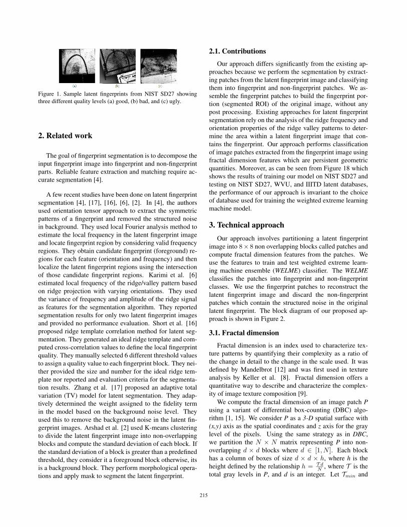
Figure 1. Sample latent fingerprints from NIST SD27 showing
three different quality levels (a) good, (b) bad, and (c) ugly.
2. Related work
The goal of fingerprint segmentation is to decompose the
input fingerprint image into fingerprint and non-fingerprint
parts. Reliable feature extraction and matching require ac-
curate segmentation [4].
A few recent studies have been done on latent fingerprint
segmentation [4], [17], [16], [6], [2]. In [4], the authors
used orientation tensor approach to extract the symmetric
patterns of a fingerprint and removed the structured noise
in background. They used local Fourier analysis method to
estimate the local frequency in the latent fingerprint image
and locate fingerprint region by considering valid frequency
regions. They obtain candidate fingerprint (foreground) re-
gions for each feature (orientation and frequency) and then
localize the latent fingerprint regions using the intersection
of those candidate fingerprint regions. Karimi et al. [6]
estimated local frequency of the ridge/valley pattern based
on ridge projection with varying orientations. They used
the variance of frequency and amplitude of the ridge signal
as features for the segmentation algorithm. They reported
segmentation results for only two latent fingerprint images
and provided no performance evaluation. Short et al. [16]
proposed ridge template correlation method for latent seg-
mentation. They generated an ideal ridge template and com-
puted cross-correlation values to define the local fingerprint
quality. They manually selected 6 different threshold values
to assign a quality value to each fingerprint block. They nei-
ther provided the size and number for the ideal ridge tem-
plate nor reported and evaluation criteria for the segmenta-
tion results. Zhang et al. [17] proposed an adaptive total
variation (TV) model for latent segmentation. They adap-
tively determined the weight assigned to the fidelity term
in the model based on the background noise level. They
used this to remove the background noise in the latent fin-
gerprint images. Arshad et al. [2] used K-means clustering
to divide the latent fingerprint image into non-overlapping
blocks and compute the standard deviation of each block. If
the standard deviation of a block is greater than a predefined
threshold, they consider it a foreground block otherwise, its
is a background block. They perform morphological opera-
tions and apply mask to segment the latent fingerprint.
2.1. Contributions
Our approach differs significantly from the existing ap-
proaches because we perform the segmentation by extract-
ing patches from the latent fingerprint image and classifying
them into fingerprint and non-fingerprint patches. We as-
semble the fingerprint patches to build the fingerprint por-
tion (segmented ROI) of the original image, without any
post processing. Existing approaches for latent fingerprint
segmentation rely on the analysis of the ridge frequency and
orientation properties of the ridge valley patterns to deter-
mine the area within a latent fingerprint image that con-
tains the fingerprint. Our approach performs classification
of image patches extracted from the fingerprint image using
fractal dimension features which are persistent geometric
quantities. Moreover, as can be seen from Figure 18 which
shows the results of training our model on NIST SD27 and
testing on NIST SD27, WVU, and IIITD latent databases,
the performance of our approach is invariant to the choice
of database used for training the weighted extreme learning
machine model.
3. Technical approachOur approach involves partitioning a latent fingerprint
image into 8× 8 non overlapping blocks called patches and
compute fractal dimension features from the patches. We
use the features to train and test weighted extreme learn-
ing machine ensemble (WELME) classifier. The WELMEclassifies the patches into fingerprint and non-fingerprint
classes. We use the fingerprint patches to reconstruct the
latent fingerprint image and discard the non-fingerprint
patches which contain the structured noise in the original
latent fingerprint. The block diagram of our proposed ap-
proach is shown in Figure 2.
3.1. Fractal dimension
Fractal dimension is an index used to characterize tex-
ture patterns by quantifying their complexity as a ratio of
the change in detail to the change in the scale used. It was
defined by Mandelbrot [12] and was first used in texture
analysis by Keller et al. [8]. Fractal dimension offers a
quantitative way to describe and characterize the complex-
ity of image texture composition [9].
We compute the fractal dimension of an image patch Pusing a variant of differential box-counting (DBC) algo-
rithm [1, 15]. We consider P as a 3-D spatial surface with
(x,y) axis as the spatial coordinates and z axis for the gray
level of the pixels. Using the same strategy as in DBC,
we partition the N × N matrix representing P into non-
overlapping d × d blocks where d ∈ [1, N ]. Each block
has a column of boxes of size d × d × h, where h is the
height defined by the relationship h = T dN , where T is the
total gray levels in P, and d is an integer. Let Tmin and
215
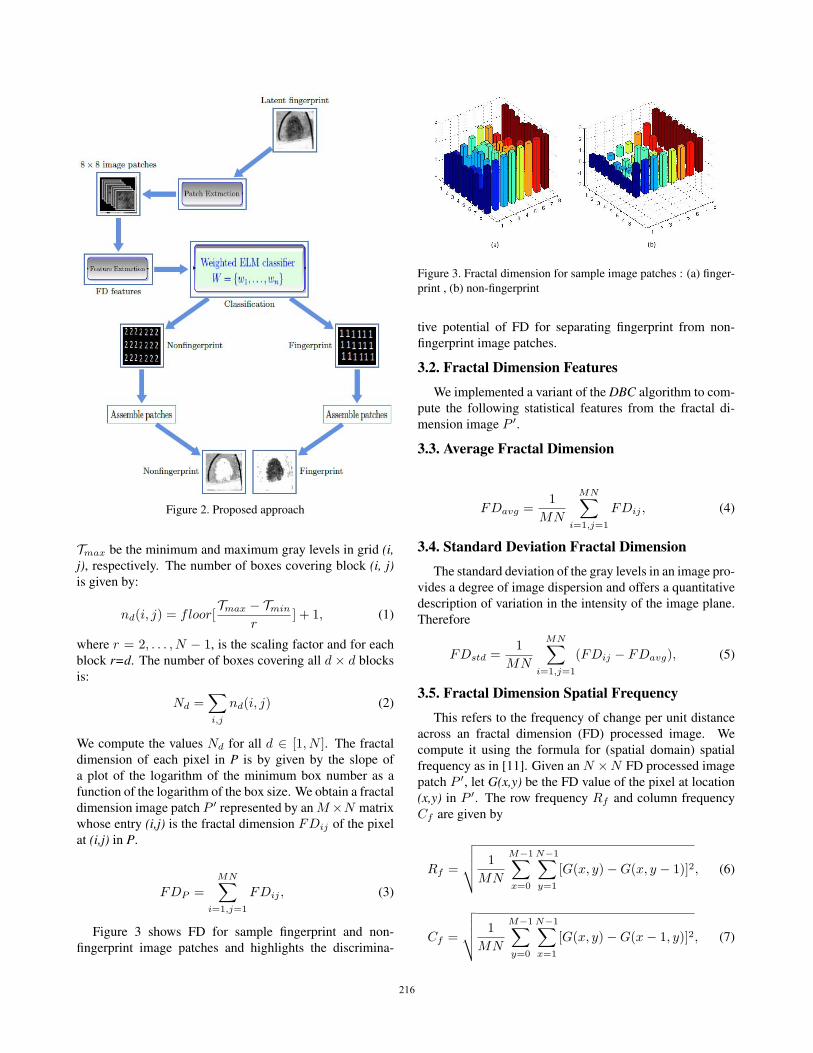
Figure 2. Proposed approach
Tmax be the minimum and maximum gray levels in grid (i,j), respectively. The number of boxes covering block (i, j)is given by:
nd(i, j) = floor[Tmax − Tmin
r] + 1, (1)
where r = 2, . . . , N − 1, is the scaling factor and for each
block r=d. The number of boxes covering all d × d blocks
is:
Nd =∑i,j
nd(i, j) (2)
We compute the values Nd for all d ∈ [1, N ]. The fractal
dimension of each pixel in P is by given by the slope of
a plot of the logarithm of the minimum box number as a
function of the logarithm of the box size. We obtain a fractal
dimension image patch P ′ represented by an M×N matrix
whose entry (i,j) is the fractal dimension FDij of the pixel
at (i,j) in P.
FDP =MN∑
i=1,j=1
FDij , (3)
Figure 3 shows FD for sample fingerprint and non-
fingerprint image patches and highlights the discrimina-
Figure 3. Fractal dimension for sample image patches : (a) finger-
print , (b) non-fingerprint
tive potential of FD for separating fingerprint from non-
fingerprint image patches.
3.2. Fractal Dimension Features
We implemented a variant of the DBC algorithm to com-
pute the following statistical features from the fractal di-
mension image P ′.
3.3. Average Fractal Dimension
FDavg =1
MN
MN∑i=1,j=1
FDij , (4)
3.4. Standard Deviation Fractal Dimension
The standard deviation of the gray levels in an image pro-
vides a degree of image dispersion and offers a quantitative
description of variation in the intensity of the image plane.
Therefore
FDstd =1
MN
MN∑i=1,j=1
(FDij − FDavg), (5)
3.5. Fractal Dimension Spatial Frequency
This refers to the frequency of change per unit distance
across an fractal dimension (FD) processed image. We
compute it using the formula for (spatial domain) spatial
frequency as in [11]. Given an N ×N FD processed image
patch P ′, let G(x,y) be the FD value of the pixel at location
(x,y) in P ′. The row frequency Rf and column frequency
Cf are given by
Rf =
√√√√ 1
MN
M−1∑x=0
N−1∑y=1
[G(x, y)−G(x, y − 1)]2, (6)
Cf =
√√√√ 1
MN
M−1∑y=0
N−1∑x=1
[G(x, y)−G(x− 1, y)]2, (7)
216
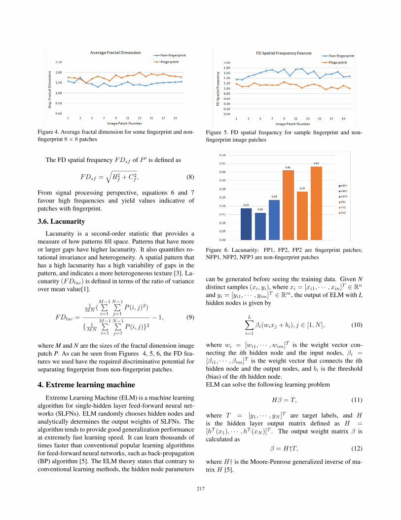
Figure 4. Average fractal dimension for some fingerprint and non-
fingerprint 8× 8 patches
The FD spatial frequency FDsf of P ′ is defined as
FDsf =√R2
f + C2f , (8)
From signal processing perspective, equations 6 and 7
favour high frequencies and yield values indicative of
patches with fingerprint.
3.6. Lacunarity
Lacunarity is a second-order statistic that provides a
measure of how patterns fill space. Patterns that have more
or larger gaps have higher lacunarity. It also quantifies ro-
tational invariance and heterogeneity. A spatial pattern that
has a high lacunarity has a high variability of gaps in the
pattern, and indicates a more heterogeneous texture [3]. La-
cunarity (FDlac) is defined in terms of the ratio of variance
over mean value[1].
FDlac =
1MN (
M−1∑i=1
N−1∑j=1
P (i, j)2)
{ 1MN
M−1∑i=1
N−1∑j=1
P (i, j)}2− 1, (9)
where M and N are the sizes of the fractal dimension image
patch P. As can be seen from Figures 4, 5, 6, the FD fea-
tures we used have the required discriminative potential for
separating fingerprint from non-fingerprint patches.
4. Extreme learning machineExtreme Learning Machine (ELM) is a machine learning
algorithm for single-hidden layer feed-forward neural net-
works (SLFNs). ELM randomly chooses hidden nodes and
analytically determines the output weights of SLFNs. The
algorithm tends to provide good generalization performance
at extremely fast learning speed. It can learn thousands of
times faster than conventional popular learning algorithms
for feed-forward neural networks, such as back-propagation
(BP) algorithm [5]. The ELM theory states that contrary to
conventional learning methods, the hidden node parameters
Figure 5. FD spatial frequency for sample fingerprint and non-
fingerprint image patches
Figure 6. Lacunarity: FP1, FP2, FP2 are fingerprint patches;
NFP1, NFP2, NFP3 are non-fingerprint patches
can be generated before seeing the training data. Given Ndistinct samples (xi, yi), where xi = [xi1, · · · , xin]
T ∈ Rn
and yi = [yi1, · · · , yim]T ∈ Rm, the output of ELM with L
hidden nodes is given by
L∑i=1
βi(wixj + bi), j ∈ [1, N ], (10)
where wi = [wi1, · · · , wim]T is the weight vector con-
necting the ith hidden node and the input nodes, βi =[βi1, · · · , βim]T is the weight vector that connects the ithhidden node and the output nodes, and bi is the threshold
(bias) of the ith hidden node.
ELM can solve the following learning problem
Hβ = T, (11)
where T = [y1, · · · , yN ]T are target labels, and His the hidden layer output matrix defined as H =[hT (x1), · · · , hT (xN )]T . The output weight matrix β is
calculated as
β = H†T, (12)
where H† is the Moore-Penrose generalized inverse of ma-
trix H [5].
217
4.1. Weighted extreme learning machine
Weighted ELM provides a solution to the classification
accuracy paradox associated with imbalance class distribu-
tion while maintaining the advantages of the unweighted
ELM. It allows for weights to be assigned to each train-
ing sample and generalizes to cost sensitive learning [18].
Specifically, we define an N×N diagonal weight W and as-
sociate it with every training sample xi. The W assigned to
a training sample xi from a minority class is larger than that
assigned to an xk from a majority class. The weight assign-
ment scheme assigns larger weight to the minority samples
thereby strengthening the impact of the minority class and
weakening the relative impact of the majority class. Gener-
ally, the goal of ELM is to minimize the training errors and
maximize the marginal distance between the classes [18]:
Minimize : ‖Hβ − T‖2 and ‖β‖ (13)
This is written mathematically as:
LpELM=
1
2‖β‖2 + C
1
2
N∑i=1
‖ξi‖2, (14)
Subject to : h(xi)β = tTi − ξTi , i = 1, . . . , N (15)
where ξi = [ξi,1, · · · , ξi,m]T is the training error vector of
m output nodes with respect to the training sample xi, Cis the regularization parameter that indicates the trade-off
between the minimization of the training errors and maxi-
mization of the marginal distance between classes, h(xi) if
the feature mapping vector in the hidden layer with respect
to sample xi, and β is the output weight vector connecting
the hidden layer and the output layer.
For the WELM, the optimization problem becomes [18]:
LpELM=
1
2‖β‖2 + CW
1
2
N∑i=1
‖ξi‖2, (16)
Subject to : h(xi)β = tTi − ξTi , i = 1, . . . , N (17)
4.2. Weighted extreme learning machine ensemble(WELME) learning
The random initialization of both the bias and input
weights of the weighted extreme learning machine causes
fluctuations in model performance between runs. By us-
ing WELME, we are able to handle large patch image data
sets and minimize the model’s empirical risk. Inspired by
[10] and [13], we implemented the WELME for fixed size
block-by-block learning and segmentation. We analytically
determined the optimal block size, which is also the number
of neurons L in the hidden layer of the WELM to be 720 as
shown in Figure 12.
We learn a set of hypothesis:
H = {f(xi, wk), wk ∈WELME} (18)
where xi is the i-th training sample and wk is the k-thWELM in the WELME. We use a non-negative real-valued
loss function L(y, y) to measure how different the predic-
tion y of a wk in the ensemble is from the true outcome y.
We compute the empirical risk associated with each hypoth-
esis h(x) by averaging the loss function on the training and
validation sets :
El(h) =1
m
m∑i=1
L(h(xi), yi) (19)
We select optimal set H∗ of hypotheses that minimizes the
total empirical risk (TER). In our experiments we let H∗
be the top 5% hypotheses that have minimal risk El(h) for
final prediction.
4.3. Voting
The final prediction from the ensemble is obtained
through voting. To obtain near optimal prediction from the
ensemble, we require that Each h(x) ∈ H∗ meet the en-
semble analytically determined confidence threshold ξ by
satisfying:
c =
FN∑i=1
Wp +
FP∑i=1
Wn ≤ ξ. (20)
ξ = min{Rv}, v = 1, . . . ,K (21)
where Rv is the total empirical risk of WELM v, K is the
number of WELMs in the ensemble, c is the total misclassi-
fication penalty for each ensemble, FN and FP are the num-
ber of false negative and false positive predictions, respec-
tively and the sum is over all the misclassification on the test
data set by a given member of the ensemble. Wp and Wn
are the weights assigned to fingerprint and non-fingerprint
patches, respectively. The weights Wp and Wn account for
the imbalance in the data set class distribution and were de-
termined analytically. In our experiments, we set ξ to the
value 0.16 which was obtained from experiments.
5. Experimental ResultsWe implemented our algorithms in Matlab R2014a run-
ning on Intel Core i7 CPU with 8GB RAM and 750GB hard
drive.
5.1. Latent fingerprint databases
We tested our model on the following databases.
NIST SD27: This database was published by the National
Institute of Standards and Technology in collaboration with
218
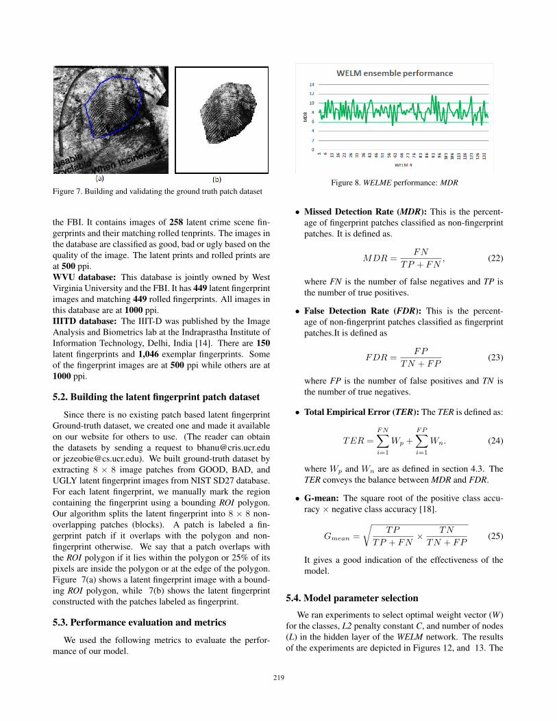
Figure 7. Building and validating the ground truth patch dataset
the FBI. It contains images of 258 latent crime scene fin-
gerprints and their matching rolled tenprints. The images in
the database are classified as good, bad or ugly based on the
quality of the image. The latent prints and rolled prints are
at 500 ppi.
WVU database: This database is jointly owned by West
Virginia University and the FBI. It has 449 latent fingerprint
images and matching 449 rolled fingerprints. All images in
this database are at 1000 ppi.
IIITD database: The IIIT-D was published by the Image
Analysis and Biometrics lab at the Indraprastha Institute of
Information Technology, Delhi, India [14]. There are 150latent fingerprints and 1,046 exemplar fingerprints. Some
of the fingerprint images are at 500 ppi while others are at
1000 ppi.
5.2. Building the latent fingerprint patch dataset
Since there is no existing patch based latent fingerprint
Ground-truth dataset, we created one and made it available
on our website for others to use. (The reader can obtain
the datasets by sending a request to [email protected]
or [email protected]). We built ground-truth dataset by
extracting 8 × 8 image patches from GOOD, BAD, and
UGLY latent fingerprint images from NIST SD27 database.
For each latent fingerprint, we manually mark the region
containing the fingerprint using a bounding ROI polygon.
Our algorithm splits the latent fingerprint into 8 × 8 non-
overlapping patches (blocks). A patch is labeled a fin-
gerprint patch if it overlaps with the polygon and non-
fingerprint otherwise. We say that a patch overlaps with
the ROI polygon if it lies within the polygon or 25% of its
pixels are inside the polygon or at the edge of the polygon.
Figure 7(a) shows a latent fingerprint image with a bound-
ing ROI polygon, while 7(b) shows the latent fingerprint
constructed with the patches labeled as fingerprint.
5.3. Performance evaluation and metrics
We used the following metrics to evaluate the perfor-
mance of our model.
Figure 8. WELME performance: MDR
• Missed Detection Rate (MDR): This is the percent-
age of fingerprint patches classified as non-fingerprint
patches. It is defined as.
MDR =FN
TP + FN, (22)
where FN is the number of false negatives and TP is
the number of true positives.
• False Detection Rate (FDR): This is the percent-
age of non-fingerprint patches classified as fingerprint
patches.It is defined as
FDR =FP
TN + FP(23)
where FP is the number of false positives and TN is
the number of true negatives.
• Total Empirical Error (TER): The TER is defined as:
TER =FN∑i=1
Wp +FP∑i=1
Wn. (24)
where Wp and Wn are as defined in section 4.3. The
TER conveys the balance between MDR and FDR.
• G-mean: The square root of the positive class accu-
racy × negative class accuracy [18].
Gmean =
√TP
TP + FN× TN
TN + FP(25)
It gives a good indication of the effectiveness of the
model.
5.4. Model parameter selection
We ran experiments to select optimal weight vector (W)
for the classes, L2 penalty constant C, and number of nodes
(L) in the hidden layer of the WELM network. The results
of the experiments are depicted in Figures 12, and 13. The
219

Figure 9. WELME performance: FDR
Figure 10. WELME performance: Empirical risk
Figure 11. WELME performance: Segmentation accuracy
optimal values are C = 105.5, L = 720, Wn = 3.75 and
Wp = 7.15 for good and bad quality images. For ugly qual-
ity images, Wn = 0.001 and Wp = 0.093. Figures 8,
9, 10, and 11 show the performance of the 134 WELMs
in the WELME in terms of MDR, FDR, empirical risk and
segmentation accuracy, respectively.
5.5. Confusion matrix
Training was done with 96,000 patches from images
from the NIST SD27 database. The test dataset consists
of 9,600 patches from the NIST SD27, WVU and IIITD la-
tent databases. The confusion matric in Figure 14 shows
Figure 12. Hyper parameter selection: accuracy in the (L) sub-
space
Figure 13. Hyper parameter selection: accuracy in the (C) sub-
space
Predicted Patch Class
Fingerprint Non-Fingerprint
Actual Patch ClassFingerprint 2061 643
Non-Fingerprint 180 6716Figure 14. Confusion matrix
the TP, TN, FP, and FN results and a segmentation accuracy
91.43%
5.6. Segmentation results
Figures 15, 16, 17 show the segmentation results of
our proposed method on sample good, bad and ugly quality
images from the NIST SD27 database. The original latent
fingerprint images are (a), (c), (e), while (b), (d), (f) are the
segmented fingerprints constructed using patches classified
as fingerprint, without any post classification processing.
220

Figure 15. Good Latent fingerprint image and segmentation result
Figure 16. Bad Latent Fingerprint Image and segmentation result.
Figure 17. Ugly Latent Fingerprint Image and segmentation result.
Figure 18 shows the performance of our approach on dif-
ferent latent fingerprint databases.
5.7. Performance comparison with other algorithms
Figure 19 highlights the superior performance of our seg-
mentation approach on the good, bad and ugly quality la-
tent fingerprints from NIST SD27 compared to the results
in [2], while Figure 20 shows that our approach performs
better than existing approaches with respect to total empir-
ical risk minimization and segmentation accuracy. Taking
both MDR and FDR into consideration, our approach is
43.72% better than that of Zhang et al. [17] on the NIST
SD27 database and 10.46% better that that of Arshad et al.
[2] on the NIST SD27 database. On the WVU database, our
approach is about 2 times better than that of Choi et al. [4].
Figure 18. Segmentation reliability in different databases for good
quality images
Figure 19. NIST SD27: Segmentation results in terms of MDRand FDR: Good, Bad, Ugly
Author Approach Database MDR % FDR % AVERAGE
Choi et al. Ridge orientation NIST SD27 14.78 47.99 31.38
and frequency
computation WVU LDB 40.88 5.63 23.26
Zhang et al. Adaptive Total NIST SD27 14.10 26.13 20.12
Variation model
Arshad et al. K-means NIST SD27 4.77 26.06 15.42
clustering
Our approach Fractal Dimension NIST SD27 9.22 18.7 13.96& Weighted ELM (Good, Bad, Ugly)
WVU LDB 15.54 9.65 12.60(Good,Bad,Ugly)
IIITD LDB 6.38 10.07 8.23
(Good)
Figure 20. Performance comparison of segmentation approaches
6. Conclusions and future work
We have proposed a new technique based on fractal di-
mension and weighted extreme learning machine (WELM)
for latent fingerprint segmentation using image patches. Ex-
perimental results using latent fingerprint images from the
NIST SD27, WVU and IIITD latent fingerprint databases
showed the promise of our method. Our future work in-
volves incorporating additional features to improve classifi-
cation accuracy of the fingerprint patches from bad and ugly
latent fingerprints.
221

References[1] O. Al-Kadi and D. Watson. Texture analysis of aggressive
and nonaggressive lung tumor ce ct images. BiomedicalEngineering, IEEE Transactions on, 55(7):1822–1830, July
2008.
[2] I. Arshad, G. Raja, and A. Khan. Latent fingerprints seg-
mentation: Feasibility of using clustering-based automated
approach. Arabian Journal for Science and Engineering,
39(11):7933–7944, 2014.
[3] M. Barros Filho and F. Sobreira. Accuracy of lacunarity al-
gorithms in texture classification of high spatial resolution
images from urban areas. In XXI congress of internationalsociety of photogrammetry and remote sensing, 2008.
[4] H. Choi, a. I. B. M. Boaventura, and A. Jain. Automatic
segmentation of latent fingerprints. In Biometrics: Theory,Applications and Systems (BTAS), 2012 IEEE Fifth Interna-tional Conference on, pages 303–310, Sept 2012.
[5] G. Huang, Q. Zhu, and C. Siew. Extreme learning machine:
Theory and applications. Neurocomputing, 70(13):489 –
501, 2006.
[6] S. Karimi-Ashtiani and C.-C. Kuo. A robust technique for
latent fingerprint image segmentation and enhancement. In
Image Processing, 2008. ICIP 2008. 15th IEEE InternationalConference on, pages 1492–1495, Oct 2008.
[7] D. Kaye, T. Busey, M. Gische, G. LaPorte, C. Aitken, S. Bal-
lou, L. B. ..., and K. Wertheim. Latent print examination and
human factors: Improving the practice through a systems ap-
proach. NIST Interagency/Internal Report (NISTIR) - 7842,
Jan 2012.
[8] J. Keller, S. Chen, and R. Crownover. Texture descrip-
tion and segmentation through fractal geometry. ComputerVision, Graphics, and Image Processing, 45(2):150 – 166,
1989.
[9] A. D. K. T. Lam and Q. Li. Fractal analysis and multifractal
spectra for the images. In Computer Communication Control
and Automation (3CA), 2010 International Symposium on,
volume 2, pages 530–533, May 2010.
[10] Y. Lan, Y. C. Soh, and G.-B. Huang. Ensemble of on-
line sequential extreme learning machine. Neurocomputing,
72(1315):3391 – 3395, 2009. Hybrid Learning Machines
(HAIS 2007) / Recent Developments in Natural Computa-
tion (ICNC 2007).
[11] S. Li, J. T. Kwok, and Y. Wang. Combination of images
with diverse focuses using the spatial frequency. InformationFusion, 2(3):169 – 176, 2001.
[12] B. Mandelbrot. The Fractal Geometry of Nature. Einaudi
paperbacks. Henry Holt and Company, 1983.
[13] B. Mirza, Z. Lin, and K.-A. Toh. Weighted online sequen-
tial extreme learning machine for class imbalance learning.
Neural Processing Letters, 38(3):465–486, 2013.
[14] A. Sankaran, M. Vatsa, and R. Singh. Hierarchical fusion
for matching simultaneous latent fingerprint. In Biometrics:Theory, Applications and Systems (BTAS), 2012 IEEE FifthInternational Conference on, pages 377–382, Sept 2012.
[15] N. Sarkar and B. B. Chaudhuri. An efficient differential
box-counting approach to compute fractal dimension of im-age. IEEE Transactions on Systems, Man, and Cybernetics,
24(1):115–120, Jan 1994.
[16] N. Short, M. Hsiao, A. Abbott, and E. Fox. Latent fingerprint
segmentation using ridge template correlation. In Imagingfor Crime Detection and Prevention 2011 (ICDP 2011), 4thInternational Conference on, pages 1–6, Nov 2011.
[17] J. Zhang, R. Lai, and C.-C. Kuo. Latent fingerprint seg-
mentation with adaptive total variation model. In Biometrics(ICB), 2012 5th IAPR International Conference on, pages
189–195, March 2012.
[18] W. Zong, G.-B. Huang, and Y. Chen. Weighted extreme
learning machine for imbalance learning. Neurocomputing,
101:229–242, 2013.
222