Lateral Stability of the Spring-Mass Hopper

Suggests a Two Step Control Strategy for Running

Sean G. Carver, Noah J. Cowan, and John M. Guckenheimer

April 5, 2009

Abstract

This paper investigates control of running gaits in the context of a spring loaded inverted

pendulum (SLIP) model in three dimensions. Specifically, it determines the minimal number

of steps required for an animal to recover from a perturbation to a specified gait. The model

has four control inputs per step: two touchdown angles (azimuth and elevation) and two spring

constants (compression and decompression). By representing the locomotor movement as a

discrete-time return map and using the implicit function theorem we show that the number of

recovery steps needed following a perturbation depends upon the goals of the control mechanism.

When the goal is to follow a straight line, two steps are necessary and sufficient for small lateral

perturbations. Multi-step control laws have a larger number of control inputs than outputs,

so solutions of the control problem are not unique. Additional constraints, referred to here as

synergies, are imposed to determine unique control inputs for perturbations. For some choices of

synergies, two step control can be expressed as two iterations of its first step policy and designed

so that recovery occurs in just one step for all perturbations for which one step recovery is

possible.

1 Introduction

Understanding locomotion demands an understanding of how the animal stabilizes

each of its gaits. What does an animal do when it inevitably finds that its state

differs from what is desired? An intriguing possibility is that the complex and high-

dimensional neuromechanical system—body, limbs, muscles, nervous system—behaves

as if it were a much lower-dimensional system [8], affording a task-level control strat-

egy to recover from perturbations “step to step” [11]. We investigate such step-to-step

1

control by examining a widely studied model of locomotion, the spring loaded inverted

pendulum (SLIP). SLIP models can describe movements of the center of mass during

running for a surprisingly wide range of species, from cockroaches to humans [4]. But

even with these reductions, a controller for SLIP would have considerable freedom

to choose its response to a given perturbation. An animal’s response likely reflects

tradeoffs between different objectives, such as stability, maneuverability and energy

efficiency; these tradeoffs undoubtedly vary between different species or within the

same animal across different behavioral contexts. An experimental investigation of

these issues demands testable hypotheses. Using a well known theorem of calculus,

namely the implicit function theorem, we study the consequences of one such hypoth-

esis: the nervous system acts to exactly correct perturbations in the minimal number

of steps.

Animal locomotion results from a complex interaction of the animal and the environment [6].

Mathematical models of this locomotor interaction typically involve differential equations predict-

ing musculoskeletal dynamics during different “continuous phases” of motion, such as free flight or

single support, together with a set of conditions, such as heel strike or toe off, that describe tran-

sitions between these continuous phases [9]. Here we present an optimal class of control strategies

for running: those that exactly correct perturbations as fast (i.e. in the fewest number of steps)

as possible. Here “exact correction” refers to the predictions of the mathematical model under

consideration. The animal need not explicitly represent this model. Our scheme requires only that

the animal learn the mapping between sensory input and the motor commands yielding the optimal

performance. This mapping can most parsimoniously be described as a solution of the nonlinear

equation that integrates the model to the desired state. The fact that many of the properties of

these control strategies can be readily understood using the implicit function theorem of calcu-

lus may not be simply fortuitous: it suggests that comparable biological strategies may exist for

learning and representing such behaviors.

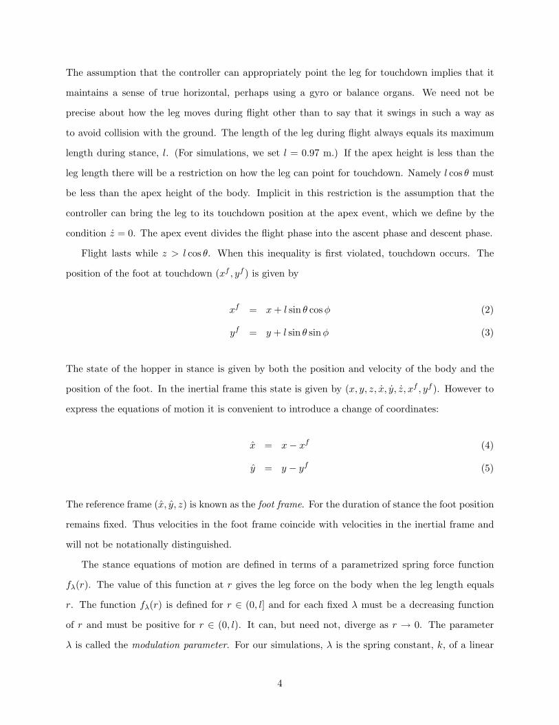
We present the main contributions of this paper in the context of a simple model for locomotion:

the spring loaded inverted pendulum (SLIP) hopper model. The SLIP model consists of a point-

mass body connected to a single massless spring-loaded leg (Figure 1). SLIP locomotion resembles

the motion of a pogo stick. Despite its simplicity, the SLIP model is widely regarded as a simple

2

description of the center-of-mass trajectory of running (and several other gaits) in diverse species

[1–4, 7, 12, 17], from humans and horses to crabs and cockroaches. As such, it is considered a

template [8, 9, 11, 15] for running. With few exceptions [5, 18, 20], most prior consideration of

SLIP restricts motion to the sagittal plane, requiring only two degrees of freedom to describe body

motion: fore–aft and up–down but not medial–lateral. Some authors have proposed templates for

running more complicated than the SLIP (for example, in the sagittal plane, [19]).

2 Modeling and control

2.1 The spring-loaded inverted pendulum (SLIP) model

We describe the spring-loaded inverted pendulum (SLIP) model used in this paper as a model of

running. Our model hopper consists of a point mass body connected to a massless spring-loaded

leg. Its motion resembles that of a pogo stick with two alternating phases: stance and flight. These

phases are distinguished by whether or not the foot (or tip of the leg) is in contact with the ground.

Transitions between these phases are called touchdowns (from flight to stance) or liftoffs (from

stance to flight).

We assume the hopper moves in a Cartesian space: three coordinates label body position from

a fixed reference. The third coordinate measures vertical height above the ground. This frame is

known as the inertial frame. During flight the state of the hopper is given only by the position

and velocity of its body (x, y, z, x, y, z). The equations of motion for the body in flight are given

by the following second order system, which determines the motion of a particle subject only to

gravitational force:

d2

dt2

x

y

z

=

0

0

−g

(1)

Because the leg is massless, its motion during flight does not affect the motion of the body.

Nevertheless its direction at the moment of touchdown does affect the subsequent stance phase: we

choose the spherical angles θ and φ determining this direction as control parameters. Here θ is the

angle (at touchdown) between the leg and downward vertical and φ is the angle (at touchdown)

between the projection of the leg onto the ground and the positive x-direction (see Figure 1).

3

The assumption that the controller can appropriately point the leg for touchdown implies that it

maintains a sense of true horizontal, perhaps using a gyro or balance organs. We need not be

precise about how the leg moves during flight other than to say that it swings in such a way as

to avoid collision with the ground. The length of the leg during flight always equals its maximum

length during stance, l. (For simulations, we set l = 0.97 m.) If the apex height is less than the

leg length there will be a restriction on how the leg can point for touchdown. Namely l cos θ must

be less than the apex height of the body. Implicit in this restriction is the assumption that the

controller can bring the leg to its touchdown position at the apex event, which we define by the

condition z = 0. The apex event divides the flight phase into the ascent phase and descent phase.

Flight lasts while z > l cos θ. When this inequality is first violated, touchdown occurs. The

position of the foot at touchdown (xf , yf ) is given by

xf = x + l sin θ cosφ (2)

yf = y + l sin θ sinφ (3)

The state of the hopper in stance is given by both the position and velocity of the body and the

position of the foot. In the inertial frame this state is given by (x, y, z, x, y, z, xf , yf ). However to

express the equations of motion it is convenient to introduce a change of coordinates:

x = x− xf (4)

y = y − yf (5)

The reference frame (x, y, z) is known as the foot frame. For the duration of stance the foot position

remains fixed. Thus velocities in the foot frame coincide with velocities in the inertial frame and

will not be notationally distinguished.

The stance equations of motion are defined in terms of a parametrized spring force function

fλ(r). The value of this function at r gives the leg force on the body when the leg length equals

r. The function fλ(r) is defined for r ∈ (0, l] and for each fixed λ must be a decreasing function

of r and must be positive for r ∈ (0, l). It can, but need not, diverge as r → 0. The parameter

λ is called the modulation parameter. For our simulations, λ is the spring constant, k, of a linear

4

spring force function whose rest length is l, but in principle one can consider other parametrized

spring laws, such as an air spring (which facilitates the generation of analytical approximations of

the stance map [17]) or a spring law that has been fitted to experimental running data [16]. For

each fixed r, fλ(r) must be an increasing function of λ. The parameter λ is set by the controller.

Modulation of the spring force during stance is required to give the controller the ability to adjust

the total energy in the system.

The stance phase is divided into the compression phase and the decompression phase by the

bottom event. At this moment the spring is maximally compressed and xx + yy + zz = 0.

In terms of fλ the equations of motion for the body in stance are given by the following second

order system:

d2

dt2

x

y

z

=

0

0

−g

+fλ(

√x2 + y2 + z2)

m√

x2 + y2 + z2

x

y

z

(6)

The above equation of motion determines the dynamics of 6 of the 8 stance state variables. The

last two stance state variables xf and yf are constant for the duration of the stance phase. Stance

lasts as long as x2 + y2 + z2 < l2. Liftoff occurs when this inequality is first violated.

We define a step as a portion of the hopper’s trajectory between two successive apexes. Five

events punctuate each step: the initial apex, touchdown, bottom, liftoff and the final apex. We

say the hopper chooses its control variables for the step at the initial apex, based on complete

knowledge of the state at that apex. We denote the space of possible apex states X. An element

of X has the form (x, x, y, y, z). It is implied that z > 0 and z = 0. Thus X = R4 × R+.

Except when we show that a more general controller cannot perform better, we say that the

modulation parameter changes once during stance, at the bottom event. We say that the controller

chooses both the compression value of the modulation parameter, kc, and the decompression value,

kd. Moreover, we assume an instantaneous transition between the compression and decompression

spring laws [17]. Thus there are four control variables for each step: (θ, φ, kc, kd). These four values

parametrize the control space U = S2 × R+ × R+.

5

2.2 Discrete time models

The class of models to which our methods apply consist of those that can be written as an iteration

of a discrete-time return (or Poincare) map, r1; see Figure 2. This map describes locomotion as the

evolution of a sequence of state-vectors, xj . These vectors are indexed by the step-number, j. In our

case, xj is the state of the SLIP at the jth apex; xj ∈ X. In a more general context, the components

of each state-vector in the sequence might be positions and velocities of each body segment, and, in

fact, might include non-mechanical states. Typically these quantities evolve continuously in time,

but we measure the state-vector at specified events, namely the apexes of the center-of-mass in

the SLIP model. These events define the boundaries between steps. The one-step return map,

r1, expresses each successive state-vector as a function of the previous step’s state-vector, and a

control-vector, uj , for the previous step:

xj+1 = r1(xj ,uj). (7)

The control vector uj quantifies the nervous system’s actions during the step j. For our controlled

SLIP, uj ∈ U .

A sequence of unperturbed reference states and corresponding control actions, (x∗j ,u∗j ), that

satisfy the return map equation:

x∗j+1 = r1(x∗j ,u∗j ). (8)

will be called a gait. While we assume that r1 is independent of the step number, note that

the reference states and the control vectors in the gait sequence may depend on j. Below, we

study neutral gaits that are defined as those gaits with the properties that x∗j+1 − x∗j and u∗j are

constant. We call a gait N -step periodic if there is a rotation R about the vertical axis so that

x∗j+N − x∗j = R(x∗j − x∗j−N ) and u∗j+N = R(u∗j ) for every j.

2.3 Deadbeat Control

The control literature gives the name deadbeat to the class of strategies that produce exact correction

to a perturbation from the target gait in a finite (usually minimal) amount of time [14]. In the

context of legged locomotion, deadbeat control means exact correction within a finite number of

6

steps. We will show that deadbeat control is feasible for a broad class of locomotion models.

The nervous system aims to stabilize a desired gait, given in general by (8). We hypothesize

that if for some j, a perturbation has left the motion off course, xj 6= x∗j , a deadbeat controller will

choose controls over the next N steps, (uj ,uj+1, . . . ,uj+N−1), for some N , to return the hopper

(exactly) to the desired motion xj+N = x∗j+N .

We assume the nervous system responds as a function of the available sensory information. For

demonstrating that a locomotion model admits a deadbeat controller, we assume that this sensory

information perfectly represents the system’s state (i.e. perfect state estimation). In this case, the

controller’s response during the subsequent N steps is a function of its state at the present step

with reference to the established target state x∗j+N of the gait:

(uj ,uj+1, . . . ,uj+N−1) = gNj (xj). (9)

The N -step return map,

xj+N = rN (xj ,uj ,uj+1, . . . ,uj+N−1), (10)

gives the state of the system at step j + N as a function of the current state and the controls over

all N steps; it can be defined recursively in terms of the N -fold composition of the one-step return

map. For example,

r2(xj ,uj ,uj+1) := r1(r1(xj ,uj),uj+1). (11)

We say that an N -step control law (for the jth step), gNj , is N -step deadbeat if for all states xj

sufficiently close to x∗j

x∗j+N = rN (xj , gNj (xj)). (12)

We also require gNj be continuously differentiable and that gN

j (x∗j ) = (u∗j ,u∗j+1, . . . ,u

∗j+N−1). In

the domain of rN , we call (x∗j ,u∗j , . . . ,u

∗j+N−1) the reference point.

The implicit function theorem [21] provides sufficient conditions for the existence of an N -step

deadbeat control law, gNj . The theorem has the following conditions (illustrated in Figure 3):

1. The control vector (uj , . . . ,uj+N−1) has the same or higher dimension than the final state

vector, xj+N .

7

2. The reference point lies in the interior of the domain of rN .

3. At the reference point rN is continuously differentiable and the Jacobian (matrix of partial

derivatives) with respect to the controls has full rank.

The deadbeat equation is a vector equation that specifies dimx∗j+N scalar conditions (equations)

x∗j+N = rN (xj ,uj ,uj+1, . . . ,uj+N−1) (13)

that must be satisfied. In this context, the desired state x∗j+N can be considered fixed and the

initial state vector, xj can be considered the “parameter” that varies as we solve for the controls

(uj ,uj+1, . . . ,uj+N−1).

The space of possible N -step controls has dimension N × dimuj . When the hypotheses of

the implicit function theorem are satisfied, N × dimuj ≥ dimx∗j+N , solutions of (13) constitute

a manifold of dimension N × dimuj − dimx∗j+N . If this difference is zero, then the implicit

theorem guarantees uniqueness of the solution in an open neighborhood of the reference point and

in neighborhoods of previously computed solutions where the theorem’s hypotheses are satisfied. If

the difference is positive, the nervous system must choose one control from the manifold of solutions.

To make this choice, we add N×dimuj−dimx∗j+N additional constraints to the deadbeat equations

(13). We call these constraints synergies (see Figure 4), in reference to muscle synergies whereby

many muscles work in concert [22]. Here, each synergy is a scalar equation involving the controls,

which together form a vector equation:

e∗ = e(uj , . . . ,uj+N−1). (14)

Once the synergies have been specified, we apply the implicit function theorem to the target

map f consisting of both the return map and the synergies:

f(xj ,uj , . . . ,uj+N−1) =

rN (xj ,uj , . . . ,uj+N−1)

e(uj , . . . ,uj+N−1)

(15)

8

In the search for controls, the deadbeat equation (13) is then replaced by

f∗j+N = f(xj ,uj , . . . ,uj+N−1), (16)

where f∗ = (x∗j+N , e∗). We choose the number of synergies to be N × dimuj − dimx∗j+N , yielding

an equation whose number of unknowns equals its number of conditions. In this situation, the

conditions of the implicit function theorem suffice to yield a (locally) unique solution of (15).

2.4 Linear Controllability and the Existence of Deadbeat Control

Suppose the return map is linear:

xj+1 = r1(xj , uj) = Axj + Buj . (17)

Let (x∗j ,u∗j ) be an unperturbed gait. A one-step deadbeat control strategy exists if for all perturbed

states xj (sufficiently close to x∗j ), there is a control uj such that

x∗j+1 = Axj + Buj . (18)

Because the equation is linear, the deadbeat control, uj , if it exists, is a linear function of xj , (i.e.

uj = g(xj) = Gxj), and the “sufficiently close” condition can be dropped. Rephrased, one-step

deadbeat control to stabilize the unperturbed gait (x∗j ,u∗j ) exists if and only if

{x∗j+1 −Axj : xj ∈ Rn} ⊂ col B, (19)

for each j, where n = dim x, and col B is the column space of matrix B.

Thus, one-step deadbeat control exists, for all gaits, if and only if rank B = n. By iterating

the equation, a similar argument shows that two-step deadbeat control exists, for all gaits, if and

only if rank [B,AB] = n, and likewise N-step deadbeat control exists for all gaits if and only

if rank [B,AB, A2B, . . . AN−1B] = n. The existence of an N for which this equation holds is

equivalent to the classical notion of controllability. Deadbeat control (for an unspecified number of

steps) exists for all gaits if and only if the system (18) is controllable.

9

2.5 Method for Numerically Computing a Nonlinear Deadbeat Control Law

Starting with the reference point or a previously computed solution (x∗j ,u∗j ,u

∗j+1, . . . ,u

∗j+N−1)

and given a specific perturbed apex state xj , we seek a solution (uj ,uj+1,uj+N−1) to the target

equation (16) that corrects the perturbation. Our search uses Newton’s method augmented with

a continuation strategy along the segment J joining x∗j to xj . When Newton’s method fails to

converge, the perturbed state xj is replaced with the midpoint of the segment joining x∗j to xj .

The replacement is closer to reference than the initial perturbed state making Newton’s method

more likely to converge. If Newton’s method converges at this new perturbed state, then the

reference, (x∗j ,u∗j ,u

∗j+1, . . . ,u

∗j+N−1), is replaced by this computed solution to the target equation.

This process is repeated to march along J , until a solution is obtained at the initial perturbed

state. Increments along J are halved when Newton’s method fails, increased by 30% when Newton’s

method converges in fewer than 4 iterations and left the same otherwise. When a planned step falls

beyond the end of J , it is reduced appropriately to reach the endpoint.

Our method can be generalized employ a parameterized curve ξ(s), instead of the segment J .

For a given curve, the implicit function theorem guarantees uniqueness of the continued solution

for sufficiently small steps in the parameter, but different curves may yield different solutions, even

if they have the same endpoints.

3 Results

Our main result is that the minimum number of steps for deadbeat control is two.

3.1 Number of Recovery Steps

One-step deadbeat control of the SLIP model is impossible because the final state vector has more

components (five) than the control vector (four). Thus the first condition of the implicit function

theorem fails. In Appendix A we show that biomechanical constraints (the fixed position of the foot

during stance) makes failure inescapable even for more complex control strategies whose control

vectors have dimension five or larger.

We illustrate a correcting maneuver requiring two steps in Figure 5. The illustration shows an

attempt to stabilize in-place hopping (i.e. running with zero forward speed). The hopper has been

10

perturbed so that its apex speed is still zero, but its apex position is shifted to the left (possibly by

an arbitrarily small amount) from its desired position. A first step of the hopper (foot placed to the

left) is required to give the hopper rightward momentum and a second placement (foot placed to the

right, shown) is required to arrest the hopper’s rightward momentum. This lane change maneuver

is required to correct perturbations arbitrarily close to the unperturbed state. It follows that the

conditions of the implicit function theorem must fail, even with additional control variables for

actuating the spring-leg. Specifically, the third condition of the implicit function theorem fails: the

Jacobian derivative of the return map r1 with respect to the controls uj does not possess full rank

at the reference point. Our demonstration of this fact in Appendix B relies on the symmetry of

the sagittal plane; however, numerical calculations indicate that one-step control is still impossible

even for trajectories that do not preserve sagittal plane symmetry, such as running around a circle.

3.2 Iteration of the First-Step Policy

Our method to obtain two-step control laws uses synergies. Different synergies can lead to qual-

itative differences in control strategy. A two-step control law schedules control action that, when

implemented, takes place over two successive steps. After one step, however, new state information

is available to the controller. If, in addition to the initial perturbation being corrected, a substantial

second perturbation occurs during the first step, it may no longer be desirable to proceed with the

initially scheduled control action for the second step. Instead, it may be desirable to start over with

a new two-step schedule. Such a new schedule would plan a maneuver to fully correct the newly

perturbed motion after two additional steps (i.e. by the end of the third step).

If repeatedly perturbed motion proceeds over many steps, the controller faces the following

choice: it can create new two-step schedules at every apex, never implementing more than the first

half of each schedule, or it can create new two-step schedules at every other apex, following each

schedule to completion. In other words, the controller can either iterate its partial first-step policy

or iterate its full two-step policy. While the former strategy always utilizes the most current state

information, its effectiveness depends upon the synergies.

11

3.3 Effect of Synergies

Both of the following sets of synergies yield locally unique control laws for two-step control of (SLIP

model) running:

synergies E1: kcj = kc

j+1 = kdj+1 = k∗. (20)

synergies E2: kcj = kd

j = kcj+1 = k∗. (21)

We emphasize that our theory requires only that synergies be continuously differentiable func-

tions; they need not be linear functions as assumed here (and below).

Synergies E1 fix the spring constant to its reference value, k∗, throughout the second step

stance phase, but allow the decompression spring constant for the first step, kdj to be adjusted. On

the other hand, synergies E2 fix the spring constant throughout the first stance phase, but allow

adjustment on the second step. A consistent value for the spring constant throughout a stance phase

implies the step conserves energy. Because the whole two-step maneuver must correct, not conserve,

energy, this correction must take place entirely during the step that does not conserve energy. In

other words, E1 corrects energy on the first step (hence the label E1) while conserving energy on

the second, whereas E2 corrects energy on the second (hence the label E2) while conserving energy

on the first. This difference has an important consequence, described below.

Suppose a controller iterates the first-step policy of one of the two-step deadbeat control laws

E1 or E2. Each iteration of the first step policy of E1 corrects energy, whereas each iteration of

the first step policy of E2 conserves energy. For the former, energy correction happens in one step;

for the latter, energy correction never happens. For synergies E2, iterating the first step policy is

clearly not an effective strategy in the face of perturbations that can change energy, for no control

action will ever change it back.

Iterating the first step policy of the control law determined by E1 does more than just correct

energy on each step. Specifically, two successive iterations of the policy, following a small perturba-

tion, will, assuming no additional perturbations, lead to an exact correction: xj+2 = x∗j+2. In other

words the iteration of the first step policy of the control law determined by E1 is itself a two-step

deadbeat control law. In Appendix C, we establish a stronger statement: the control law given by

12

two iterations of the first step policy of E1 is actually the same as the control law determined by

the full two-step policy. In other words, for synergies E1, following the new schedule is the same as

following the old, assuming that no additional perturbations change how the controller evaluates

the new policy. On the other hand, if an additional perturbation has occurred, clearly the first

step policy is more appropriate because it accounts for the new state information. With no further

perturbations, iterating the first step policy corrects motion in two additional steps, whereas if the

controller waits a step to create a new schedule, it takes three additional steps.

We say that the control law determined by E1 is expressible as an iteration of its first step

policy. See Figure 6 for a graphical depiction of this property.

3.4 Control Laws Illustrated

We explored the domains of two-step deadbeat control laws for running with the spatial SLIP model.

These studies are based upon a neutral gait with parameters fit to the motion of a human sprinter,

as reported by [13] for a population of eight young adult male athletes who were not sprint running

specialists. To fit the data, we used eight conditions obtained in [13] by averaging across steps

and/or subjects. We used three trajectory conditions (contact time per step equals 0.110 s, flight

time per step equals 0.141 s, and velocity during contact equals 8.1 m/s), two anthropomorphic

conditions (mass equals 72.7 kg, leg length equals 0.97 m), and three neutral conditions (all apexes

have the same speed and height and there is no lateral motion). The conditions determined the

parameters m, and l, the reference control variables θ∗, φ∗, and k∗ (necessarily equal for all steps,

and such that k∗,d = k∗,c), and components of the reference apex state (speed and height, equal

for all steps). These constraints together with the arbitrary choices x∗0 = y∗0 = y∗0 = 0, x∗0 > 0,

uniquely determined the entire reference trajectory.

Our results are displayed in Figures 7, 8 and 9. To produce the bitmaps in the background

of these figures, we applied our numerical algorithm (Section 2.5) to calculate the control law on

a regularly spaced mesh of perturbations within a two-dimensional slice of the five-dimensional

initial apex state space. Specifically, within our slice, x and y (respectively, the in-line and lateral

components of initial position) varied, while z (the initial hopping height) and x, and y remained

constant and equal to their reference values. Because the implicit function theorem only guar-

antees local uniqueness of the target equations, we employed a continuation strategy to map the

13

solution manifold and search for multiple solutions. Within the slice, we continued the solutions

along sequences of intermediate points, following one of four directions, and stopping when the

continuation failed to produce a solution. The four directions chosen were: increasing x, decreasing

x, increasing y and decreasing y, where in each direction we held everything else constant.

The algorithm proceeded to explore, within the slice, the region where deadbeat control could

be defined. The location within the slice determines the initial apex state for the motion; the

algorithm computes the control action (leg pointing and spring constants over two steps) needed to

produce motion that satisfies the deadbeat condition at the end of the motion. If no such control

action exists, the algorithm will fail. We interpreted the failure points as the boundaries of the

deadbeat control law. We ran our algorithm until the region had been maximally expanded to

failure points in all four chosen directions from all mesh points. For selected boundary points we

verified that a condition of the implicit function theorem failed (for example, see caption to Figures

8 and 9). The white space in the figure represents apex states that are beyond the boundary

of the deadbeat control law. The color gradient indicates how close the correction is to one-step

correction. More precisely, the green saturation is determined by the two-norm distance in five

dimensional apex state space between the first corrected apex in the two-step maneuver and the

corresponding reference apex, where most saturated indicates perfect one-step correction. Note

that this two-norm metric involves a scaling between position and velocity that our units (m and

m/s) determine arbitrarily.

We considered two control laws that differed in their synergies: synergies E1 (Figures 7 and 8,

defined by (20)), as well as the following synergies (Figure 9), which we call synergies G:

θj+1 = θ∗, kcj+1 = kd

j+1 = k∗ (22)

In Appendix C we show that synergies G, like the synergies E1, determine control laws that are

expressible in one step (that is, they are equal to two iterations of their first step, barring additional

perturbations, as discussed above). Moreover the control law determined by synergies G, while

having a smaller domain of definition than the one determined by synergies E1, has a desirable

property, shown in Appendix C: the control law determined by synergies G is greedy (hence the label

G) in the sense that it always (for all small perturbations) selects a maneuver that achieves exact

14

correction in the fewest number of steps possible. For this two-step control law, greedy means that

the synergies always select a maneuver that exactly corrects perturbations in one step, whenever

such a maneuver exists. When a two-step control law corrects in one step, the second step that the

correcting maneuver specifies coincides with the reference trajectory.

When can a perturbation be corrected in one step? For the SLIP example, most lateral pertur-

bations (that is, a generic set) cannot be corrected in one step, however some can. First, consider

the two-step maneuver depicted in Figure 5. The initial apex, like most other perturbed apex

states, cannot be corrected in one step. However the motion can be corrected in one step from the

middle apex of the correcting maneuver. The control laws determined by both synergies E1 and

synergies G, given that they are both one-step expressible, correct in one step all states that can be

reached as middle apexes of a two-step correcting maneuver determined by the same control law.

Second, all small perturbations that preserve the sagittal plane can be corrected in one step—by

a maneuver that is locally unique (near the reference point). We discovered this fact by verifying

numerically that the conditions of the implicit function theorem for one-step correction hold within

the invariant sagittal plane. As shown in Appendix C, for all small perturbations, synergies G

select the unique one-step correcting maneuver—indeed, as noted above, they select a one-step

correction whenever such a maneuver exists. On the other hand, synergies E1 typically select a

maneuver that requires two steps to accomplish exact correction for sagittal perturbations, despite

the existence of a one-step maneuver that corrects exactly. Figure 9 plots the reference trajectory

and two correcting maneuvers for the control law determined by synergies G. The initial apexes

of all displayed trajectories lie within the sagittal plane, and for both correcting maneuvers, the

correction is exact in one-step: both correcting maneuvers have second steps that coincide with the

reference trajectory.

The correcting trajectories for synergies E1 and synergies E2 coincide when the correction

conserves energy, for example for perturbations that change only x and/or y. In this case (as

shown in Figures 7 and 8) perturbations are corrected with trajectories that are mirror symmetric

about the middle apex.

The reference trajectory and two example correcting maneuvers from synergies E1 are shown

in Figure 8. (However, in all cases shown, the correcting maneuvers from synergies E1 and from

synergies E2 coincide.) The two correcting maneuvers plotted have the same initial apex, despite

15

the fact that they follow different trajectories. This situation is allowed by the fact that the domain

of definition of the control law determined by synergies E1 is not simply connected (meaning that

some closed paths are not deformable to a point while staying within the domain). The fact that

the two-dimensional slice shown is not simply connected is apparent from the holes in Figure 7.

Note in Figures 7 and 8 that the dark green annulus extends below the bright green tongue on

which the reference point lies. Where the two overlap, the control law determined by synergies E1

is nonunique. However, note that only the solution depicted by the bright green tongue is local to

the reference point; although both a “bright green” and a “dark green” maneuver can correct the

unperturbed initial condition, the controls for these maneuvers are separated and local uniqueness

near the reference point still holds.

3.5 Less Restrictive Control Targets

Up to this point we have considered SLIP locomotion patterns that place a target value on all five

components of the apex state: (x, x, y, y, z). Because these targets constrain in-line position, x, as

well as other quantities, they might be appropriate for a runner trying to step squarely on marks

on a track, spaced according to the preferred step length of the runner. Alternatively, these targets

might apply to a long jumper on the last few steps before reaching the takeoff boards. However,

runners don’t ordinarily care where they step in relation to marks on the ground and, in this more

common situation, it is unlikely that the in-line position of the apex state is under deadbeat control.

A simple modification to our scheme allows for an appropriate generalization. We write the target

function (from (15)), not in terms of the value of the return map, but in terms of the value of the

return map projected via a function h onto a (possibly) lower dimensional surface in the apex state

space:

f(xj ,uj ,uj+1, . . . ,uj+N−1) =

h(r(xj ,uj ,uj+1, . . . ,uj+N−1))

e(uj ,uj+1, . . . ,uj+N−1)

(23)

We call the components of the projection h, the correction criteria. If h is the identity function

(as before) then we say h implements trajectory correction, because all components of the trajectory

are controlled. Alternatively, for path correction of a neutral gait, h drops the x component from

the value of r, appropriate if the runner does not care about hypothetical marks on the ground.

16

What other sets of correction criteria are there? We might consider compass correction, which

drops both components of horizontal position: x and y. These correction criteria would be ap-

propriate for running in a straight line without a specified target, where perturbations in lateral

position need not be corrected. Compass correction assumes that the controller has an intrinsic

sense of direction, derived either from a compass or from a view of distant landmarks. Deadbeat

control for compass correction can be achieved with a one-step control law, whereas path correction,

like trajectory correction, requires two steps to correct lateral perturbations.

Note that when the number of conditions is changed by the correction criteria, the number of

synergies must change accordingly.

3.6 Other Gaits and Maneuvers

We have analyzed deadbeat control of the neutral gait. This gait is periodic, with a one step period,

and the motion of the center of mass remains in a consistent sagittal plane. However we emphasize

that deadbeat control can stabilize other, more complicated, motions.

Consider that a human runner has two legs and therefore, in reality, the motion has a period

of at least two steps (one stride). If the motion of the center of mass does not remain within the

sagittal plane but shifts laterally back and forth, (e.g. depending upon what leg is on the ground),

as the runner advances, we call such a gait an alternating gait. We considered the possibility

that breaking the symmetry associated with the sagittal plane by switching from a neutral to an

alternating gait would allow one-step deadbeat control, but discovered that the SLIP model with an

alternating gait still requires two-steps for deadbeat path correction of most small perturbations.

While the alternating gait has a two step period, there are non-neutral gaits that have a one step

period, including circle hopping, back-and-forth hopping and in-place hopping. For circle hopping,

the body’s height and speed remain the same at each apex, but the direction changes by a constant

angle from apex to apex. Consequently, the apexes of the desired motion fall equidistant from some

center point (i.e. they lie on a circle). Back-and-forth and in-place hopping are degenerate forms

of circle hopping. For back-and-forth hopping the turning angle is 180◦ and the desired apexes

alternate between two states with the same position and speed, but opposite direction of motion.

For in-place hopping the circle radius is zero, all desired apex states coincide, the forward apex

speed is zero, and the apex directions of motion are not defined uniquely. We have tested the

17

SLIP model with a circle gait and a correction criteria that constrain height, tangential and radial

velocity, and distance to the center point, but not position along the circle. We discovered that

this circle gait path correction requires two steps to correct perturbations.

For non-periodic gaits, i.e. maneuvers, the reference apex state, the reference control, the syner-

gies, and the correction criteria all depend on step number, giving a step dependent target function

for N -step deadbeat control:

fj(xj ,uj ,uj+1, . . . ,uj+N−1) =

hj(r(xj ,uj ,uj+1, . . . ,uj+N−1))

ej(uj ,uj+1, . . . ,uj+N−1)

(24)

When the conditions of the implicit function theorem hold, the target function implicitly deter-

mines a step-dependent multistep deadbeat control law gNj . That is, for all xj in the neighborhood

of the unperturbed xj , the deadbeat equation is satisfied:

fj(xj , gNj (xj)) = f∗j+N (25)

Assuming such a gNj exists, all step-dependent targets will be satisfied, N -steps after a sufficiently

small perturbation on the jth apex, provided the controller applies the N -step control chosen at

the jth apex, and provided no additional perturbations occur.

As an example of a non-periodic maneuver to be deadbeat stabilized, consider a lane change.

Suppose it is desired to shift to a parallel lane between the jth and j + 2nd apexes, but otherwise

run in a straight line with a specified hopping height. Similar maneuvering has been studied in

ostriches [10]. The simplest way to accomplish this maneuver with a deadbeat-controlled SLIP is

with a shift in the control law. For example, during the first j−1 steps, the control law for running

illustrated by Figures 7 and 8 can be applied, then for all subsequent steps the same control law,

but with shifted desired lateral positions y∗j , y∗j+1, . . . , can be applied. To be feasible, the desired

(unshifted) apex state xj must lie within the domain of definition of the shifted control law. Note

that this control law is expressible in one step: for each step of the control law, it is only the first

step of the two step maneuver that is applied.

Note that the sudden shift does not fit the framework of (24) and (25) on every step. Specifically

the shift is not taken into account on the j − 1st step. If a perturbation occurs at apex xj−1, the

18

two step correction will be appropriate for the old control law and will not correct the motion to

arrive after two steps at the intermediate apex of the maneuver xj+1, as in the above framework.

If the runner expects the lane change, one may want to formulate an appropriate control law on

the j − 1 step: g2j−1. This formulation will not change the desired motion but will change the way

perturbations on the j − 1st step are corrected.

4 Discussion

We have analyzed feedback control strategies for stabilizing running that correct perturbations

to a target trajectory in a minimal number of steps. Our strategy for closing the loop feedback

suggests hypotheses for the nervous system’s response to a range of perturbations, including those

with a lateral component. While it is known that the spatial spring-loaded inverted pendulum

(SLIP) requires feedback for stability [20], little experimental work considers the control of human

or animal running in this context. In the absence of data to challenge our model, it makes sense to

use the SLIP formulation to generate predictions that can be tested with experiment. However, our

contributions do not rely upon the validity of the closed-loop SLIP model. Rather, our hypothesis

states that the equation expressing the “exact correction” of some model’s motion describes the

nervous system’s control law that closes the loop. As perhaps the simplest such model, the SLIP

model produces parsimonious predictions. Nonetheless, most of our conclusions with the SLIP

model illustrate more general truths that hold for exact correction of other locomotion models. The

mathematical assumptions required to make these conclusions hold for a broad class of models.

The implicit function theorem framework we advance for studying locomotion is quite broad.

It allows freedom in specifying the correction criteria for determining the control targets and the

synergies for resolving redundancy. Nevertheless, one specific testable hypothesis can be posed to

guide future experimental work: control targets are met in the minimal number of steps. Consid-

ering only perturbations without a lateral component, our model, as we have formulated it, admits

just one set of synergies with the hypothesized greedy property (for trajectory correction). Unfor-

tunately, in a more realistic model of locomotion, e.g. with continuous actuation of many joints and

muscles, many sets of synergies will be consistent with our hypothesis. How are synergies chosen?

Perhaps synergies reflect evolutionary tradeoffs between stability, maneuverability, and energy ef-

19

ficiency that reflect unique conditions for each species. Comparative studies should be informative

in this regard.

Often, the problem of relating control systems models to experimental locomotion data becomes

one of parameter fitting: find the feedback gains for a particular closed-loop model that minimize

error between observed and numerically simulated system trajectories. Necessarily such models

directly couple requirements on sensory systems with demands on the motor output. A deadbeat

controller, by contrast, has no feedback control gains to tune. Instead, these controllers can be

described by a parametrized family of control synergies and correction criteria, which can themselves

be directly fitted to data. We suspect that the resulting correction criteria will provide insight into

requirements on sensory systems, i.e. what the nervous system needs to measure, while the resulting

control synergies describes the space of motor actions the nervous system can take in order to drive

this measurement to its control target.

A Lane Change Corrections Require At Least Two Steps

First we will show that one class of perturbations, those requiring a “lane change” (see Figure

5) for recovery, can never be corrected in one step. Because lane changes are required for some

arbitrarily small lateral perturbations to the neutral gait, one-step deadbeat control for the neutral

gait does not exist.

We consider any gait which maintains a consistent sagittal plane. A lane change is required if

a perturbation leaves the velocity vector parallel to the desired plane at apex, but offsets the body

position. For the SLIP model we show that a maneuver that corrects such a perturbation requires

at least two steps.

In the interest of clarity, Figure 5 shows a lane change for in-place hopping, a degenerate neutral

gait where the desired forward speed is zero. In this scenario, the desired trajectory lies on a vertical

line, but perturbations can still occur along all five dimensions of apex state space. A lane change

is required if the perturbed speed at apex is zero (same as with the unperturbed speed), but the

body does not lie on the desired vertical line. Similar reasoning shows that two steps are required

for lane changes stabilizing in-place hopping and neutral hopping.

Our key assumption is that the hopper maintains single point of contact with the ground that

20

cannot move during stance. For a more realistic model of human running, with a foot of nonzero

size, small lane changes might be possible in one step, but not if the distance between the lanes is

greater than the width of the foot.

Suppose the perturbed state (body at initial apex) lies to the left of the desired state at the

origin: y0 < y∗ = 0. Furthermore, suppose that the lateral velocity is zero, as desired: y0 = y∗ = 0.

The following assumption is superfluous but makes the reasoning conceptually simpler: we assume

motion is constrained to the desired frontal (yz) plane (that is, there is never any motion in the

fore/aft direction): x(t) = x(t) = x∗ = x∗ = 0. The controller wishes to place the foot, yf , to

return the hopper to the goal after one step: y1 = y1 = 0.

Is this maneuver possible? Note the forward invariance of the following regions of state space

1. yf < y(t) and y(t) ≥ 0,

2. yf > y(t) and y(t) ≤ 0, and

3. yf = y(t) and y(t) = 0.

The invariance follows from the fact that the leg force (the only nonvertical force on the body) is

always directed from the foot to the body, and from the fact that the foot cannot move.

Because the body must move to the right to return to the goal, it follows that the foot must

be placed so that yf < y0. But then the state cannot remain on or return to the boundary of the

invariant region where y = 0. Thus recovery in one step is impossible: at least one additional step

will be necessary to arrest the hopper’s rightward movement and return the hopper to the goal.

B Failure of Implicit Function Theorem for One-Step Correction

As the model has been formulated, one-step deadbeat control with trajectory correction does not

exist because there are more control targets (five) than control variables (four). Thus the system

violates condition 1 of the implicit function theorem. But what about one-step path correction

(with only four targets) or one-step trajectory correction with more actuation control of the leg

spring (at least five control variables). Condition 1 no longer fails, but note that in these cases,

for the neutral gait, lane changes will still be necessary for some arbitrarily small perturbations.

21

The reasoning in Appendix A shows that deadbeat control (for these scenarios) still does not exist.

Which condition of the implicit function theorem fails? We will show condition 3 fails.

Recall for the neutral gait that the desired trajectory maintains a consistent sagittal plane.

Choose the x-axis as the constant horizontal direction of motion. Then the condition y = y = 0

determines the sagittal plane, which can be parametrized by the remaining state variables (x, x, z).

We call these remaining state variables sagittal variables, and the other variables, y and y, medi-

olateral variables. On the other hand, we call the control variables θj and all leg force actuation

variables k(i)j sagittal controls, and call φj mediolateral controls

Let Jms be the Jacobian derivative of the mediolateral variables with respect to the sagittal

controls and define Jss, Jsm, and Jmm analogously. The sagittal controls leave the sagittal plane

invariant. Thus Jms = 0 (i.e. Jms equals the zero matrix of the appropriate dimension). By

symmetry about the sagittal plane, Jsm = 0. Let Ju be the Jacobian derivative of the return map

(r1 or r2) with respect the controls and suppose the variables and controls have been properly

ordered to give Ju the block structure:

Ju =

Jss 0

0 Jmm

(26)

Then Ju is the matrix that must have full rank to satisfy condition 3. Since Ju has as many

columns as rows (by condition 1), each diagonal block must have rank equal to the number of its

rows. For one step deadbeat control (return map is r1) full rank is impossible because Jmm has

two rows (corresponding to yj+1 and yj+1) whereas it has only one column (corresponding to φj).

For two-step deadbeat control (return map is r2) there are still two rows (corresponding to yj+2

and yj+2), but now two columns (corresponding to φj and φj+1).

C Consequences of Local Uniqueness

Consider the two-step deadbeat control, (uj ,uj+1), chosen following a perturbation of the initial

apex state xj . Assuming no additional perturbations, the motion recovers after two steps: xj+2 =

x∗j+2. Thus the control chosen at this j + 2nd apex will be the reference control for two steps:

(uj+2,uj+3) = (u∗,u∗). To show the control law is expressible as its first step policy, we show that

22

the two-step deadbeat control that would be chosen by iterating the first step policy at apex xj+1

coincides with (uj+1,u∗). As it turns out, this demonstration can be accomplished easily: as long

as (uj+1,u∗) satisfies the synergy conditions, the conclusion follows from the uniqueness enforced

by synergies. All that is needed to show that (uj+1,u∗) satisfies the synergy conditions is (1) to

verify the implication that if uj+1 satisfies the second step conditions then it satisfies the first step

conditions and (2) to verify that u∗ satisfies the second step conditions. Note that both of these

statements hold for both synergies E1 and synergies G, respectively, but not for synergies E2.

Our demonstration of one-step expressibility has a gap which we now fill: the synergies only

imply local uniqueness. As above, we note that whenever (uj ,uj+1) satisfies the synergies then

(uj+1,u∗) satisfies the synergies. In addition, note that whenever (uj ,uj+1) is close to (u∗,u∗)

then (uj+1,u∗) is close to (u∗,u∗). It follows that the two-step control law must locally (in an open

neighborhood of the reference point) be the same as the iteration of its first step, which is all we

will be able to conclude.

A similar argument shows the greediness of synergies G. Note that all the conditions for synergies

G involve constraints on the second step control variables, allowing complete freedom for all first

step control variables. Moreover, synergies G fix the second step controls to their reference values.

Therefore (uj ,u∗) always satisfies the synergy conditions. Because synergies G determine the

control uniquely, if the control uj corrects the perturbation, i.e. if

x∗j+1 = r1(xj ,uj), (27)

then (uj ,u∗) must be the unique two-step control selected by the synergy conditions to correct the

perturbed apex state xj . Again the same caveat applies: we can only conclude local greediness.

Specifically, there exists an open neighborhood O of the reference point (x∗j ,u∗j ,u

∗j+1) such that if

O contains a one step correction—that is a point (xj ,uj) satisfying (27), then (uj ,u∗) must be the

unique two-step control chosen by synergies G to correct xj .

23

Acknowledgments

We thank our collaborators, Jusuk Lee, Julia Choi and Amy Bastian, for fruitful discussions. Andy

Ruina provided helpful feedback and direction in the early phases of this work. This work was

supported by the National Science foundation under Grants NSF 0101208, NSF 0425878, and

0543985.

24

References

[1] R. Altendorfer, D. E. Koditschek, and P. Holmes. Stability analysis of a clock-driven rigid-body

SLIP model for RHex. Int. J. Robot. Res., 23(10-11):1001–1012, 2004.

[2] R. Altendorfer, D. E. Koditschek, and P. Holmes. Stability analysis of legged locomotion

models by symmetry-factored return maps. Int. J. Robot. Res., 23(10-11):979–999, 2004.

[3] R. Blickhan. The spring-mass model for running and hopping. J Biomech, 22(11-12):1217–27,

1989.

[4] R. Blickhan and R. J. Full. Similarity in multilegged locomotion: Bouncing like a monopode.

J. Comp. Physiol. A, 173:509–517, 1993.

[5] S. G. Carver. Control of a Spring Mass Hopper. PhD thesis, Cornell University, 2003.

[6] M. H. Dickinson, C. T. Farley, R. J. Full, M. R. Koehl, R. Kram, and S. L. Lehman. How

animals move: An integrative view. Science, 288(5463):100–106, 2000.

[7] C. T. Farley, J. Glasheen, and T. A. McMahon. Running springs: speed and animal size. J.

Exp. Biol., 185:71–86, 1993.

[8] R. J. Full and D. E. Koditschek. Templates and anchors: neuromechanical hypotheses of

legged locomotion on land. J. Exp. Biol., 202(23):3325–3332, 1999.

[9] P. Holmes, R. J. Full, D. Koditschek, and J. Guckenheimer. The dynamics of legged locomotion:

Models, analyses, and challenges. SIAM Rev., 48(2):207–304, 2006.

[10] D. L. Jindrich, N. C. Smith, K. Jespers, and A. M. Wilson. Mechanics of cutting maneuvers

by ostriches (struthio camelus). J. Exp. Biol., 210:1378–1390, 2007.

[11] J. Lee, S. N. Sponberg, O. Y. Loh, A. G. Lamperski, R. J. Full, and N. J. Cowan. Templates

and anchors for antenna-based wall following in cockroaches and robots. IEEE Trans. Robot.,

24(1):130–143, Feb. 2008.

[12] T. A. McMahon and G. C. Cheng. The mechanics of running: how does stiffness couple with

speed? J Biomech, 23 Suppl 1:65–78, 1990.

25

[13] J.-B. Morin, T. Jeannin, B. Chevallier, and A. Belli. Spring-mass model characteristics during

sprint running: correlation with performance and fatigue-induced changes. Int J Sports Med,

27(2):158–165, Feb 2006.

[14] G. A. Perdikaris. Computer Controlled Systems: Theory and Applications. Kluwer Academic

Pubishers, 1991.

[15] U. Saranli and D. E. Koditschek. Template based control of hexapedal running. In Proc. IEEE

Int. Conf. Robot. Autom., volume 1, pages 1374–1379, Taipei, Taiwan, September 2003.

[16] W. J. Schwind. Spring Loaded Inverted Pendulum Running: A Plant Model. PhD thesis,

University of Michigan, 1998.

[17] W. J. Schwind and D. E. Koditschek. Approximating the stance map of a 2-dof monoped

runner. J. Nonlinear Science, 10(5):533–568, 2000.

[18] J. Seipel and P. Holmes. Three-dimensional translational dynamics and stability of multi-

legged runners. Int. J. Robot. Res., 25(9):889–902, September 2006.

[19] J. Seipel and P. Holmes. A simple model for clock-actuated legged locomotion. Regular and

Chaotic Dynamics, 12:502–520, 2007.

[20] J. E. Seipel and P. Holmes. Running in three dimensions: Analysis of a point-mass sprung-leg

model. Int. J. Robot. Res., 24:657–674, 2005.

[21] M. Spivak. Calculus on Manifolds: A modern approach to classical theorems of advanced

calculus. Addison-Wesley Publishing Company, 1965.

[22] L. H. Ting and J. M. Macpherson. A limited set of muscle synergies for force control during

a postural task. J. Neurophysiol., 93(1):609–613, Jan 2005.

26

Figure 1: Diagram of spring-loaded inverted pendulum (SLIP) hopper. Motion is allowed in allthree dimensions. Shown are positional coordinates of the body together with the variables thatdetermine the pointing of the leg.

27

-3 -2 -1 0 1 2 30.5

0.6

0.7

0.8

0.9

1

1.1

1.2

1.3

1.4

1.5

Desired

Too High

Too Low

Descent

Compression Decompression

Ascent

Initial

Vertical Velocity of the Body (m/s)

Ve

rtic

al P

ositio

n o

f th

e B

od

y (

m)

Figure 2: State space and trajectories of the SLIP, with motion constrained to a vertical line. Thestate variables under this constraint are vertical position of the body (vertical axis) and verticalvelocity of the body (horizontal axis). The four quadrants represent the four phases of motion ofthe SLIP (in order from apex: descent, compression, decompression, and ascent). The hopper isin flight when the vertical position of the body is greater than 1 (the uncompressed leg length).The quadrant boundaries are the event conditions (respectively, touchdown, bottom, liftoff andapex). The thick vertical line (in flight, vertical velocity 0) is the Poincare section defining apex,parametrized by a single variable (vertical body position at apex or hopping height). We assumethat trajectories start and stop on this section. In this example, the controller acts by changingthe decompression spring constant at bottom. Trajectories with different possible controls divergefrom this point. Some reach subsequent apex states that are too low (red), some that are two high(blue), and for one particular value of the control (the deadbeat control), the subsequent apex statereaches its desired height (green). If the initial height were different (but within some range), thedeadbeat control would also be different, but would still exist (not shown).

28

0

10

20

30

40

1.0 1.2 1.4 1.6 1.8 2.00

10

20

30

40

1.0 1.2 1.4 1.6 1.8 2.0

De

co

mp

ressio

n S

prin

g C

on

sta

nt (k

N/m

)

Vertical Position of Body at Apex (m)

A B

C D

Figure 3: An illustration of the conditions of the implicit function theorem and how they can fail.The horizontal axis in each panel is the initial apex state (initial hopping height from Figure 2).The vertical axis is the applied control (decompression spring constant, see Figure 2). The bluedashed curves represent the level sets of the Poincare return map (the locus of initial apex statesand controls which send the hopper to a point with a particular apex height on the next step).The thick blue curve is the level set corresponding to the desired final height. In other words, ifthe control (or decompression spring constant), is chosen so that the corresponding point on thisgraph lies on the thick blue curve, then the subsequent apex has the desired height, see Figure 2.(Note that only the vertical location on the graph can be chosen by the controller—the horizontallocation is determined by the initial apex height.) Thus the thick blue curve is the graph of thedeadbeat control law (deadbeat control as a function of the initial apex state). The asterisk is thereference point that defines the unperturbed reference motion. Red curves indicate hypotheticalboundaries of the return map. A: All conditions of the implicit function theorem hold and thedeadbeat control law can be defined for apex states in an open neighborhood (lower thick blue line)of the reference initial apex state (asterisk). B-D: The deadbeat control law cannot be defined in anopen neighborhood of the reference point because the conditions of the implicit function theoremfail. B: The control is constrained to have only one value. Thus there is one target (or conditionon the final apex state) and a smaller number (zero) of unknowns. C: The reference point lies onthe boundary of the return map—boundaries have been arbitrarily created for this purpose. D:A hypothetical return map having level sets whose projection to apex states has folds—thus theJacobian derivative of the return map with respect to the control has less than full rank. Thedeadbeat control law cannot be defined in an open neighborhood of a reference point on the fold.

29

De

co

mp

ressio

n S

prin

g C

on

sta

nt (k

N/m

)

Synergy 1

Syn

erg

y 2

Syn

erg

y 3

10 12 14 16 18 20 22 24 26 28 3010

12

14

16

18

20

22

24

26

28

30

Compression Spring Constant (kN/m)

Figure 4: An illustration of possible synergies for the 1-step control of vertical hopping whereboth the compression and the decompression spring constants remain free to be chosen by thecontroller. Shown is the space of possible controls (the pair of compression and decompressionspring constants). Each colored line corresponds to an initial hopping height and the line is thelocus of controls that achieve the deadbeat targets (final hopping height of 1.3 m). Synergies selectexactly one point on each colored line (in other words, select a control law—a deadbeat controlfor each possible initial height). In this case only one synergy is needed. Synergy 1, kd = 15,fixes the decompression spring constant, leaving the compression spring constant free. Likewise,Synergy 2, kc = 15, fixes the compression spring constant, as in Figures 2 and 3. Synergy 3,kd + 0.4(kc − 10)2 = 25, covaries the two control variables along a different prescribed path. Allthree synergies intersect at the reference control for the unperturbed periodic motion (red asterisk).Periodic motion results from any control value on the diagonal kc = kd. (The diagonal is also theline corresponding to an initial height equal to the desired height). The motion being stabilizeddetermines the reference control (asterisk).

30

Initial Apex Final ApexApex

Shadow of

Initial Apex

Shadow of

Final Apex

First Footprint Second Footprint

Figure 5: A two-step maneuver that accomplishes a lane change for in place hopping, an easy-to-visualize degenerate running gait with zero forward speed. The degenerate “lanes” in this case arepoints on the ground (shadows of the initial and final apexes). The left most blue circle representsthe perturbed apex state; the rightmost blue circle represents the final desired apex state. Boththe initial and final states have zero horizontal velocity. The first step gives the hopper rightwardmomentum. The second step arrests the rightward momentum. Because the center of pressurecannot move during stance, two steps are required to make this correction, no matter how closethe perturbed and desired states lie. Blue circles on the ground represent the projections of theinitial and final apex states. Asterisks represent foot location. The trajectory is divided betweenblue (flight) and red (stance).

31

Figure 6: An illustration of closed-loop control with a two-step deadbeat control law that is ex-pressible in one step. The space shown is analogous to the apex state space. The closed-loopreturn map projects the entire space onto the line (x, y) : y = 0 (labeled (x, 0) with the functionf(x, y) = (y, 0). The funnels illustrate this projection. The seven lines are the preimages of sevenarbitrarily chosen points (asterisks) that map to the goal in one more step. Two iterations of thisreturn map sends all points to the goal at the origin: f ◦ f(x, y) = f(y, 0) = (0, 0).

32

x

y

1m

Figure 7: A two-dimensional slice of the domain of the deadbeat control law determined by synergiesE1. Of the five components of initial apex state space, the plot shows only perturbations of in-lineand lateral position; the other components are fixed at their reference values. The SLIP’s referencemotion is from left to right on the plot. White space indicates regions outside the control law’sdomain (i.e. where continuation fails). Note that the domain is not simply connected allowingnonuniqeness (the bright green “tongue” partially occludes the dark green “annulus”). Darkershades of green indicate a larger distance (2-norm) to the reference trajectory as measured betweenapexes after the first step of the motion. Brightest green (the reference point) represents zerodistance (i.e. one step correction). Darkest green represents maximal distance (2-norm = 17.33).Superimposed on this plot are five trajectories from different selected initial perturbations. Bluecurves: body in flight, red curves: body in stance, blue circles: body at apex, red asterisks: footplacement fixed during stance. Despite large initial differences, all trajectories coincide by the endof the second step.

33

0.5m

A

B

C

yz

x

yz

x

yz

x

Figure 8: Three trajectories implementing the deadbeat control law determined by synergies E1.The bitmaps in these panels are enlargements of the central region of the bitmap in Figure 7. A: Thereference trajectory. B and C: Initially perturbed trajectories with coinciding initial conditions. B:The trajectory closer to one-step deadbeat (measured as for the color gradient). C: The trajectoryfarther from one-step correction. Upper subpanels show each trajectory in the xy-plane where theunperturbed motion is positively directed along the x-axis. Lower subpanels show the trajectory inxz-plane. The boundary near the initial condition in B is a fold. As the boundary near the initialcondition in C is approached, the duration of the middle flight phase tends to zero and the firstliftoff coincides with the second touchdown.

34

A

B

C

yz

x

yz

x

yz

x

0.5m

Figure 9: Three trajectories implementing the deadbeat control law determined by synergies G.The plots have the same axes as the corresponding ones in Figure 8, but differ as noted. A: Thereference trajectory (same as in Figure 8). B: A trajectory initially retarded along the line ofmotion. C: A trajectory initially advanced along the line of motion. All trajectories shown haveinitial conditions in the sagittal plane thus the second step of the trajectories in both B and Ccoincides with the reference motion in A (one-step correction). Top panels: the brightest shadeof green (x-axis) represents one-step correction. Away from this axis the distance from one-stepcorrection falls off slowly at first then rapidly close to the boundary. The colors scheme is analogous,but the narrow band of darkest green at the lateral boundaries represents only a 2-norm distanceof about 1/20 of the 2-norm distance of the same shade in Figure 7. As the boundary near theinitial condition in B is approached, a weak spring constant allows the leg to fully compress so thatthe body reaches the foot. On the other hand, as the boundary near the initial condition in C isapproached, two pairs of events coincide. First, the initial apex approaches the first touchdownand, second, the first liftoff approaches the first corrected apex.

35

-3 -2 -1 0 1 2 30.5

0.6

0.7

0.8

0.9

1

1.1

1.2

1.3

1.4

1.5

Desired

Too High

Too Low

Descent

Compression Decompression

Ascent

Initial

Vertical Velocity of the Body (m/s)

Verti

cal P

ositi

on o

f the

Bod

y (m

)

0

10

20

30

40

1.0 1.2 1.4 1.6 1.8 2.00

10

20

30

40

1.0 1.2 1.4 1.6 1.8 2.0

Dec

ompr

essi

on S

prin

g C

onst

ant (

kN/m

)

Vertical Position of Body at Apex (m)

A B

C D

Dec

ompr

essi

on S

prin

g C

onst

ant (

kN/m

)

Synergy 1

Synergy 2

Synergy 3

10 12 14 16 18 20 22 24 26 28 3010

12

14

16

18

20

22

24

26

28

30

Compression Spring Constant (kN/m)

Initial Apex Final ApexApex

Shadow ofInitial Apex

Shadow ofFinal Apex

First Footprint Second Footprint

x

y

1m

0.5m

A

B

C

yz

x

yz

x

yz

x

A

B

C

yz

x

yz

x

yz

x

0.5m