lateral transport of sediment and organic ... - epic.awi.de · dr. rer. nat lucas kämpf / tu...

Faculty of Environmental Sciences Institute of Soil Science and Site Ecology

Master’s Thesis

Lateral transport of sediment and organic matter, derived

from coastal erosion, into the nearshore zone of the southern

Beaufort Sea, Canada

Submitted by: B. Sc. Gregor Pfalz

Matriculation number: 3563979

Water Management

Potsdam, March 28th 2017

Supervisors: Dr. Michael Fritz / Alfred-Wegener-Institut

Dr. rer. nat Lucas Kämpf / TU Dresden

Responsible professor: Prof. Dr. Karl-Heinz Feger

Faculty of Environmental Sciences Institute of Soil Science and Site Ecology

Description of Master’s thesis topic (Aufgabenstel lung für die Masterarbeit) Name: Gregor Pfalz Born: 10.07.1989 Matriculation Num.: 3563979

Subject: “Lateral transport of sediment and organic matter, derived from coastal erosion, into the nearshore zone of the southern Beaufort Sea, Canada”

Research Statement

According to Gruber (2012), 25% of Earth’s land surfaces are affected by permafrost, which is extremely vulnerable to climate change. Especially the Arctic region with its permafrost coasts is among one of “[…] the most rapidly warming areas of the globe over the past several decades” (IPCC, 2007). Therefore, coastal erosion with high erosion rates, due to accelerated thawing and responses to environmental forcing, are of great concern.

The Alfred Wegener Institute - Helmholtz Centre for Polar and Marine Research - in Potsdam focusses in one of its projects on assessing the transport and degradation pathways of sediment and organic matter from erosion at the coastline until deposition on the sea floor. The study area for this project is the southern Beaufort Sea region as it is characterized by high coastal erosion rates and organic carbon contents, making it a key area for coastal change in the Arctic (Lantuit and Pollard, 2008).

Herschel Basin is a natural depression on the southern Beaufort Shelf, which is located in the western Canadian Arctic between the Mackenzie Delta and the Alaskan border. The submarine basin of late Wisconsin age is a natural sediment trap for material eroded along the Yukon coast and through its unique position within the area also a valuable paleoenvironmental archive. During a field campaign in spring 2016, a thirteen meter long sediment core was obtained from the Herschel Basin.

The main objective of this Master’s thesis is to quantify the amount of carbon, nitrogen and sediment with terrestrial origin throughout the sediment column from the Herschel Basin. Furthermore, correlations shall be established between different geochemical parameters. The data from such analyses will be used to determine the material sources of the Herschel Basin deposits.

Supervisors: Dr. Michael Fritz (Alfred-Wegener-Institut, Potsdam)

Dr. rer. nat. Lucas Kämpf (Technische Universität Dresden)

Hand Out: 01.11.2016

Duration: 31.03.2017

Prof. Dr. Karl-Heinz Feger

1. Gruber, S. (2012): Derivation and analysis of a high-resolution estimate of global permafrost zonation, The Cryosphere, 6, 221-233 2. IPCC (2007): Climate change 2007: the physical science basis. Contribution of Working Group I to the Fourth Assessment Report of

the Intergovernmental Panel on Climate Change, Cambridge Univ. Press, Cambridge 3. Lantuit, H & Pollard, WH (2008): Fifty years of coastal erosion and retrogressive thaw slump activity on Herschel Island, southern

Beaufort Sea, Yukon Territory, Canada. Geomorphology 95, 84-102.

Annex to the Master’s thesis topic of Gregor Pfalz

Detailed description of the master thesis

Goal: To quantify the amount of carbon, nitrogen and sediment with terrestrial background

in the Herschel Basin

Material: A 13 m long sediment core from a central position in Herschel Basin

Methods: * Determination of density and magnetic susceptibility through multi-sensor core

logger

* Preparation and identification of calcareous macrofossils for AMS 14C dating

* Determination of carbon and nitrogen concentration

* Determination of stable carbon isotopes ( δ13C)

* Grain size analysis

* Literature review

Expected Results:

(1) Only a part of the organic carbon and nitrogen stored in the coastal permafrost is accumulated

in the marine sediment record of the Herschel Basin

(2) The biogeochemical quality of the eroded carbon changes from the source of the erosion to

the accumulation in the basin, i.e. organic carbon will be selectively degraded based on

biological availability

(3) High accumulation rates on the shelf remove substantial amounts of carbon from the Arctic

carbon cycle

(4) Only the fine-grained proportion of the eroded sediment reaches the center of the basin

Organizational Issues

The laboratory analyses and investigations shall be adapted in their extent to the temporal limitation of the thesis in such a way that a closed result is presented. The thesis should be written in English. Two hardcopies of the thesis have to be submitted to TU Dresden. Additional hardcopies might be agreed with the supervisors. Additionally at least the following parts have to be delivered as file: abstract, key words, passport photo (JPEG). The results of the work have to be summarized as theses. Consultations with the supervisors are indispensable. The oral presentation is coordinated with the supervisors and the responsible professor.

I

INDEX OF TABLES ............................................................................................................................................. II

INDEX OF FIGURES .......................................................................................................................................... III

ABSTRACT ....................................................................................................................................................... IV

1. INTRODUCTION ....................................................................................................................................... 1

MOTIVATION ............................................................................................................................................. 1 1.1. ACHIEVEMENTS OF THIS THESIS ...................................................................................................................... 3 1.2. THESIS STRUCTURE ...................................................................................................................................... 3 1.3.

2. STUDY AREA ............................................................................................................................................ 4

GEOGRAPHICAL AND GEOLOGICAL SETTING ...................................................................................................... 4 2.1.2.1.1. Permafrost and periglacial environment ...................................................................................... 4 2.1.2. Herschel Island and the development of the Herschel Basin ........................................................ 7 DESCRIPTION OF THE MODERN SITUATION ....................................................................................................... 9 2.2.

2.2.1. Climate .......................................................................................................................................... 9 2.2.2. Currents and possible inflows ..................................................................................................... 10 2.2.3. Coastal processes and environmental forcing ............................................................................ 13

3. METHODS .............................................................................................................................................. 16

EQUIPMENT ............................................................................................................................................ 17 3.1. APPLIED LABORATORY METHODS ................................................................................................................. 19 3.2.

3.2.1. Non-destructive methods ............................................................................................................ 19 3.2.2. Destructive methods ................................................................................................................... 22

4. DATA ANALYSIS ..................................................................................................................................... 32

VISUAL CONDITION ................................................................................................................................... 32 4.1. MAGNETIC SUSCEPTIBILITY ......................................................................................................................... 32 4.2. GRAIN SIZE ANALYSIS ................................................................................................................................. 33 4.3. WATER CONTENT ..................................................................................................................................... 37 4.4. TOTAL ORGANIC CARBON AND TOC/TN RATIO ............................................................................................... 38 4.5.

Δ13

C ...................................................................................................................................................... 39 4.6.

Δ13

C VS. TOC/TN RATIO ........................................................................................................................... 41 4.7.

14C DATING ............................................................................................................................................. 42 4.8.

5. DISCUSSION ........................................................................................................................................... 44

6. CONCLUSION ......................................................................................................................................... 52

7. REFERENCES ........................................................................................................................................... 54

APPENDIX .................................................................................................................................................... A

TABLE OF CONTENTS

II

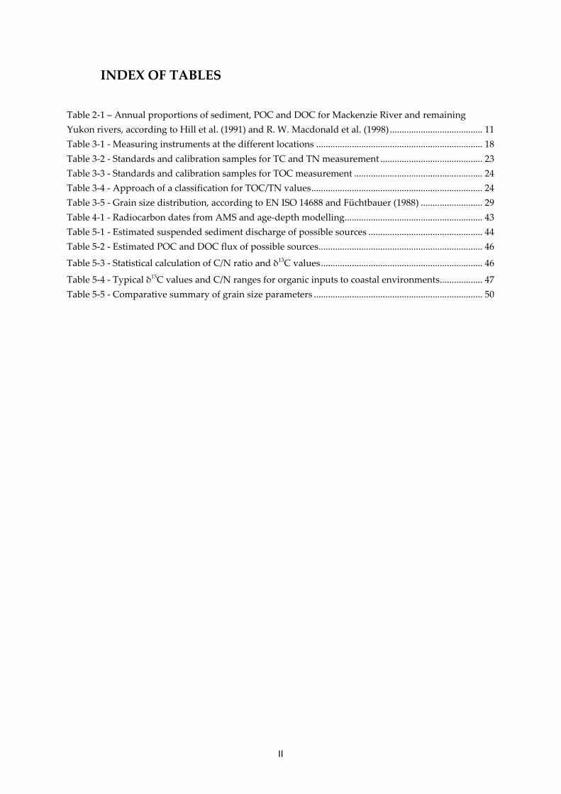
Table 2-1 – Annual proportions of sediment, POC and DOC for Mackenzie River and remaining Yukon rivers, according to Hill et al. (1991) and R. W. Macdonald et al. (1998) ....................................... 11 Table 3-1 - Measuring instruments at the different locations ...................................................................... 18 Table 3-2 - Standards and calibration samples for TC and TN measurement ........................................... 23 Table 3-3 - Standards and calibration samples for TOC measurement ...................................................... 24 Table 3-4 - Approach of a classification for TOC/TN values ........................................................................ 24 Table 3-5 - Grain size distribution, according to EN ISO 14688 and Füchtbauer (1988) .......................... 29 Table 4-1 - Radiocarbon dates from AMS and age-depth modelling .......................................................... 43 Table 5-1 - Estimated suspended sediment discharge of possible sources ................................................ 44 Table 5-2 - Estimated POC and DOC flux of possible sources ..................................................................... 46

Table 5-3 - Statistical calculation of C/N ratio and δ13C values .................................................................... 46

Table 5-4 - Typical δ13C values and C/N ranges for organic inputs to coastal environments.................. 47 Table 5-5 - Comparative summary of grain size parameters ....................................................................... 50

INDEX OF TABLES

III

Figure 1-1 - Permafrost extent in the Northern Hemisphere ......................................................................... 1 Figure 1-2 - “Impact of thaw and erosion of Arctic permafrost coasts” ....................................................... 2 Figure 2-1 - Location of study area in the surrounding topography ............................................................ 4 Figure 2-2 - Idealized latitudinal distribution of permafrost characteristics from northwestern Canada .......................................................................................................................................... 6 Figure 2-3 - Distinct bathymetric regions of study area .................................................................................. 8 Figure 2-4 - Change of annual temperature in 2015 compared to 1961-1990 average & “Mean monthly temperature and precipitation for Komakuk Beach and Shingle Point, Yukon Territory” ....................... 9 Figure 2-5 - “Study area with official names of places and feature” modified with longshore currents ............................................................................................................................................. 10 Figure 2-6 - “Sediments Pour from Mackenzie River into Beaufort Sea, Canada on November 11th, 2010” ....................................................................................................................................... 12 Figure 2-7 - “Arctic coastal processes and responses to environmental forcing” ..................................... 13 Figure 2-8 - Coastal processes: Thermal abrasion, Thermal denudation, Sea-ice processes .................... 15 Figure 3-1 - Schematic flow chart of laboratory methods ............................................................................. 16 Figure 3-2 - Piston corer system used for this expedition............................................................................. 17 Figure 3-3 - Sampling gadget and its functionality ....................................................................................... 17 Figure 3-4 - Schematic plan of Multi-Sensor Core Logger ............................................................................ 18 Figure 3-5 - Calibration liner filled with aluminum and water ................................................................... 20 Figure 3-6 - Solving the issue by the momentum of the magnetic field ..................................................... 21 Figure 3-7 - Flow diagram of methods for elementary analysis .................................................................. 22 Figure 3-8 - Flow diagram of method for δ13C analysis ................................................................................ 25

Figure 3-9 - Attribution of isotopic δ13C values and atomic C/N ratios to their origin ........................... 26 Figure 3-10 - Flow diagram of method for grain size analysis..................................................................... 28 Figure 3-11 - Macrofossils from segment “PG 2303-6 277 cm” .................................................................... 31 Figure 4-1 - Photograph of segment PG 2303-6 (100 – 200 cm) .................................................................... 32 Figure 4-2 - Magnetic susceptibility data from PG 2303 ............................................................................... 33 Figure 4-3 - Grain size distribution of PG 2303 .............................................................................................. 34 Figure 4-4 - Grain size distribution of core segment PG 2303 - 2 ................................................................ 34 Figure 4-5 - Classification of PG 2303, according to sediment triangle by Shepard (1954) ...................... 35 Figure 4-6 - Arithmetic mean grain size for PG 2303 as well as the distribution of Sand, Silt and Clay ........................................................................................................................................................ 36 Figure 4-7 - Water content of PG 2303 ............................................................................................................. 37 Figure 4-8 - TOC values in percent and TOC to TN ratio for PG 2303 ....................................................... 38

Figure 4-9 - δ13C values of PG 2303 .................................................................................................................. 40

Figure 4-10 - Attribution of isotopic δ13C values and atomic C/N ratios of PG 2303 ................................ 41 Figure 4-11- Age-depth model of PG 2303 ...................................................................................................... 42 Figure 5-1 - “Circum-Arctic map of coastal erosion rates”........................................................................... 45

INDEX OF FIGURES

IV

Herschel Basin is a natural depression on the southern Beaufort Shelf, which is located in the western Canadian Arctic between the Mackenzie Delta and the Alaskan border. The submarine basin of late Wisconsin age is a natural sediment trap for material eroded along the Yukon coast and through its unique position within the area also a valuable paleoenvironmental archive. During a field campaign in spring 2016, a thirteen meter long sediment core was obtained from the Herschel Basin.

The aim of this Master’s thesis was to quantify the amount of carbon, nitrogen and sediment with terrestrial origin throughout the sediment column from the Herschel Basin. The increasing research effort to understand the dynamics of Arctic coasts is justified by their contribution to the global carbon budget and their vulnerability.

The results showed that the majority of sediment found in the sediment column of the Herschel Basin could be assigned to a mix of riverine and terrestrial/coastal inputs. However, the individual percentage of each input (marine, fluvial and terrestrial) could not be distinguished, due to lack of data.

In conclusion, this thesis showed that in the Arctic nearshore zone coastal erosion affected by climate change will definitely have a negative impact on “[…] climate feedbacks, on nearshore food webs, and on local communities, whose survival still relies on marine biological resources”(M. Fritz et al., 2017).

Keywords: Herschel Basin, climate change, Yukon Coast, coastal erosion, accumulation of sediment

Hypotheses

(1) Only a part of the organic carbon and nitrogen stored in the coastal permafrost is accumulated in the marine sediment record of the Herschel Basin.

(2) The biogeochemical quality of the eroded carbon changes from the source of the erosion to the accumulation in the basin, i.e. organic carbon will be selectively degraded based on biological availability.

(3) High accumulation rates on the shelf remove substantial amounts of carbon from the Arctic carbon cycle.

(4) Only the fine-grained proportion of the eroded sediment reaches the center of the basin, whereas the large portion of eroded material will be transported through, for instance, currents, ice push, or resuspension to different locations.

ABSTRACT

V

Statement of original authorship

German:

Hiermit erkläre ich an Eides statt, dass ich die vorliegende Arbeit selbstständig und ohne fremde Hilfe angefertigt habe. Sämtliche benutzten Informationsquellen sowie das Gedankengut Dritter wurden im Text als solche kenntlich gemacht und im Literaturverzeichnis angeführt. Die Arbeit wurde bisher nicht veröffentlicht und keiner Prüfungsbehörde vorgelegt.

English:

The work contained in this thesis has not been previously submitted for a degree or diploma from any other higher education institution to the best of my knowledge and belief. The thesis contains no material previously published or written by another person except where due reference is made.

Gregor Pfalz

Date: / /

1

Motivation 1.1.

A changing climate has always been present in Earth’s history, especially when considering glacial and interglacial periods. Due to anthropogenic influences, however, this natural oscillation has been altered in an unprecedented way, and is still changing with only partially predictable consequences for some regions of the world. (cf. IPCC et al. (2013) and Ruddiman (2013))

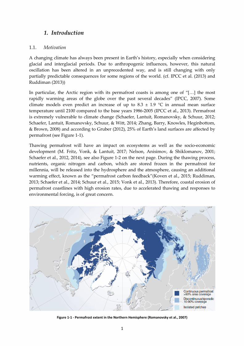
In particular, the Arctic region with its permafrost coasts is among one of “[…] the most rapidly warming areas of the globe over the past several decades” (IPCC, 2007). Some climate models even predict an increase of up to 8.3 ± 1.9 °C in annual mean surface temperature until 2100 compared to the base years 1986-2005 (IPCC et al., 2013). Permafrost is extremely vulnerable to climate change (Schaefer, Lantuit, Romanovsky, & Schuur, 2012; Schaefer, Lantuit, Romanovsky, Schuur, & Witt, 2014; Zhang, Barry, Knowles, Heginbottom, & Brown, 2008) and according to Gruber (2012), 25% of Earth’s land surfaces are affected by permafrost (see Figure 1-1).

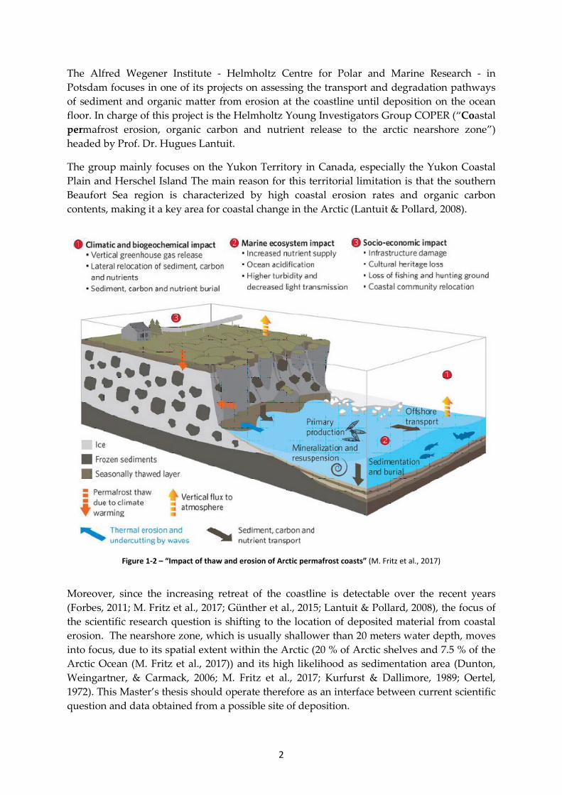
Thawing permafrost will have an impact on ecosystems as well as the socio-economic development (M. Fritz, Vonk, & Lantuit, 2017; Nelson, Anisimov, & Shiklomanov, 2001; Schaefer et al., 2012, 2014), see also Figure 1-2 on the next page. During the thawing process, nutrients, organic nitrogen and carbon, which are stored frozen in the permafrost for millennia, will be released into the hydrosphere and the atmosphere, causing an additional warming effect, known as the “permafrost carbon feedback”(Koven et al., 2015; Ruddiman, 2013; Schaefer et al., 2014; Schuur et al., 2015; Vonk et al., 2013). Therefore, coastal erosion of permafrost coastlines with high erosion rates, due to accelerated thawing and responses to environmental forcing, is of great concern.

Figure 1-1 - Permafrost extent in the Northern Hemisphere (Romanovsky et al., 2007)

1. Introduction

2

The Alfred Wegener Institute - Helmholtz Centre for Polar and Marine Research - in Potsdam focuses in one of its projects on assessing the transport and degradation pathways of sediment and organic matter from erosion at the coastline until deposition on the ocean floor. In charge of this project is the Helmholtz Young Investigators Group COPER (“Coastal permafrost erosion, organic carbon and nutrient release to the arctic nearshore zone”) headed by Prof. Dr. Hugues Lantuit.

The group mainly focuses on the Yukon Territory in Canada, especially the Yukon Coastal Plain and Herschel Island The main reason for this territorial limitation is that the southern Beaufort Sea region is characterized by high coastal erosion rates and organic carbon contents, making it a key area for coastal change in the Arctic (Lantuit & Pollard, 2008).

Figure 1-2 – “Impact of thaw and erosion of Arctic permafrost coasts” (M. Fritz et al., 2017)

Moreover, since the increasing retreat of the coastline is detectable over the recent years (Forbes, 2011; M. Fritz et al., 2017; Günther et al., 2015; Lantuit & Pollard, 2008), the focus of the scientific research question is shifting to the location of deposited material from coastal erosion. The nearshore zone, which is usually shallower than 20 meters water depth, moves into focus, due to its spatial extent within the Arctic (20 % of Arctic shelves and 7.5 % of the Arctic Ocean (M. Fritz et al., 2017)) and its high likelihood as sedimentation area (Dunton, Weingartner, & Carmack, 2006; M. Fritz et al., 2017; Kurfurst & Dallimore, 1989; Oertel, 1972). This Master’s thesis should operate therefore as an interface between current scientific question and data obtained from a possible site of deposition.

3

Achievements of this thesis 1.2.

The main objective of this Master’s thesis is to quantify the amount of carbon, nitrogen and sediment with terrestrial origin throughout the sediment column from the Herschel Basin. Therefore, it is imperative to evaluate the obtained core by its existing layers. Furthermore, correlations shall be established between different geochemical parameters. The data from such analyses will be used to determine the material sources of the Herschel Basin deposits. Moreover, the potential causal connection between the sedimentation rate and climate change will be discussed.

For this thesis the following hypotheses were established beforehand:

(1) Only a part of the organic carbon and nitrogen stored in the coastal permafrost is accumulated in the marine sediment record of the Herschel Basin.

(2) The biogeochemical quality of the eroded carbon changes from the source of the erosion to the accumulation in the basin, i.e. organic carbon will be selectively degraded based on biological availability.

(3) High accumulation rates on the shelf remove substantial amounts of carbon from the Arctic carbon cycle.

(4) Only the fine-grained proportion of the eroded sediment reaches the center of the basin, whereas the large portion of eroded material will be transported through, for instance, currents, ice push, or resuspension to different locations.

Thesis structure 1.3.

The following chapter, which will be carried out based on a literature search, comprises the study area as well as the influential factors of the surrounding area. This will later support the discussion and the assumptions made by the obtained data. Thereafter, the third chapter describes the methodical procedure of the laboratory work, and includes a brief description of the fieldwork.

The results obtained from the laboratory work are presented in Chapter 4, “Data analysis”. Following this chapter, the discussion will evaluate the data in the context of other studies as well as the study area itself. In the final chapter, conclusions will be drawn and further research recommended.

4

Geographical and geological setting 2.1.

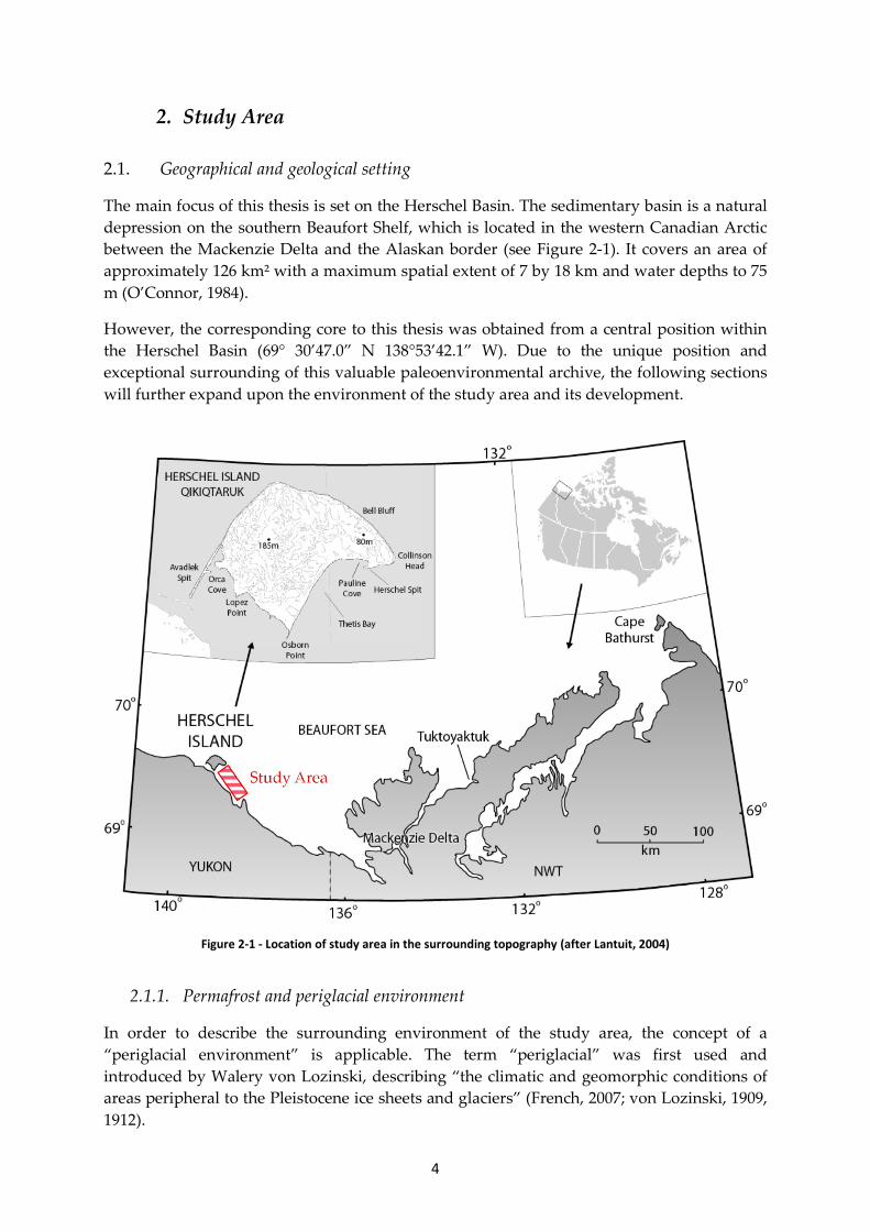
The main focus of this thesis is set on the Herschel Basin. The sedimentary basin is a natural depression on the southern Beaufort Shelf, which is located in the western Canadian Arctic between the Mackenzie Delta and the Alaskan border (see Figure 2-1). It covers an area of approximately 126 km² with a maximum spatial extent of 7 by 18 km and water depths to 75 m (O’Connor, 1984).

However, the corresponding core to this thesis was obtained from a central position within the Herschel Basin (69° 30’47.0” N 138°53’42.1” W). Due to the unique position and exceptional surrounding of this valuable paleoenvironmental archive, the following sections will further expand upon the environment of the study area and its development.

Figure 2-1 - Location of study area in the surrounding topography (after Lantuit, 2004)

2.1.1. Permafrost and periglacial environment

In order to describe the surrounding environment of the study area, the concept of a “periglacial environment” is applicable. The term “periglacial” was first used and introduced by Walery von Lozinski, describing “the climatic and geomorphic conditions of areas peripheral to the Pleistocene ice sheets and glaciers” (French, 2007; von Lozinski, 1909, 1912).

2. Study Area

5

Nowadays, “periglacial” is used to refer to a broader range of processes in cold, non-glaciated regions regardless of their proximity to glaciers or ice sheets (French, 2007; Van Everdingen, 2005). Nevertheless, two criteria were established to identify periglacial environments (French, 2007):

(1) “A freeze-thaw oscillation is dominant” (Tricart, 1968), due to water-related frost action processes, which is leads to transformations of the landscape through frost heave and subsidence, frost cracking / mechanical weathering as well as material sorting.

(2) The presence of perennially frozen ground (i.e. permafrost), since it is “the common denominator of the periglacial environment” (Péwé, 1969).

Permafrost is, by definition, ground material, i.e. rock, soil, or unconsolidated sediment (including organic material and ice), that remains at or below 0°C for at least two consecutive years (R. J. E. Brown & Kupsch, 1974; French, 2007; Van Everdingen, 2005). As mentioned in the introduction, approximately 25% of the Earth’s land surface is affected by permafrost (French, 2007; Gruber, 2012; Zhang et al., 2008).

The growth, thickness and distribution of permafrost over the world depend on a negative, thermodynamic heat balance at the surface, between surface and ground temperature (Pollard, 1998). However, this heat balance is controlled by air temperature and geothermal gradient (French, 2007; Pollard, 1998), which, by implication, are determined by regional climate, vegetation, snow / ice cover, sediment composition and its moisture content as well as topographic features (French, 2007; Washburn, 1979).

The distribution of permafrost can further be classified into three major types, due to the fact that permafrost is not limited to high latitude landscapes, but also present in mountainous areas in lower latitudes and large areas of the continental shelves of the Arctic Ocean (Romanovsky et al., 2007) (see also Figure 1-1). The zones are classified as follows (French, 2007; Romanovsky et al., 2007; Weise, 1983):

a. Continuous permafrost: Continuous permafrost covers 90 up to 100 percent of an affected area, except beneath large rivers and deep lakes. This zone occurs in areas where the annual mean temperature is less than or equal to -8 °C – often found in high latitudes of the Northern hemisphere – and a thin snow cover is predominant that favors permafrost through an isolation effect. The genesis of this type of permafrost took place during or after the last glacial period.

b. Discontinuous permafrost: The discontinuous permafrost covers 50 to 90 percent of an area and is often interrupted by taliks (unfrozen ground). It can be found towards lower latitudes as it is a remnant of continuous permafrost and/or in the process of degradation. It is also discussed that the discontinuous permafrost “is much younger and formed within the last several thousand years”(Romanovsky et al., 2007).

c. Sporadic and isolated permafrost: The last type of permafrost is the sporadic and isolated permafrost, which could cover an area from less than 10 up to 50 percent. It is characterized by single patches of frozen ground in an otherwise unfrozen area, which represents an advanced stage in degradation.

6

Figure 2-2 - Idealized latitudinal distribution of permafrost characteristics from northwestern Canada

(Heginbottom, Brown, Humlum, & Svensson, 2012)

As mentioned before, permafrost is affected by periodic (daily, seasonal, or decadal) freeze and thaw oscillations (French, 2007; French & Shur, 2010). The uppermost ground layer, also known as the “active layer” (see Figure 2-2), is exposed to those cycles directly (Van Everdingen, 2005). Therefore, the thickness of the active layer can vary significantly in time and space (French, 2007), depending on the factors affecting the heat balance.

In discontinuous permafrost the active layer is interrupted by taliks, which are layers or bodies of unfrozen ground (French, 2007; Van Everdingen, 2005). There are three variations of talik, which could be distinguished (Heginbottom et al., 2012; Van Everdingen, 2005):

a. Closed talik: Positioned within the permafrost body and completely surrounded by permafrost;

b. Open talik: Also surrounded by permafrost, but open at either the bottom or the top to an unfrozen layer;

c. Through-going talik: Interconnected to other unfrozen layers, separating active layer and permafrost vertically.

7

About 50 percent of the area of Canada is underlain by permafrost (French, 2007; Heginbottom et al., 2012); while almost the entire study area is affected by continuous permafrost (see Figure 1-1). According to GSC (Geological Survey Canada) and USGS (United States Geological Survey), the nearshore zone of the Beaufort Sea is also affected by subsea permafrost (Brothers, Herman, Hart, & Ruppel, 2016; Hu, Issler, Chen, & Brent, 2013; Ruppel, Herman, Brothers, & Hart, 2016). However, the data for the Herschel basin are only sparsely available, which is why subsea permafrost will not be further discussed in this thesis.

2.1.2. Herschel Island and the development of the Herschel Basin

The name of the basin originates from the nearby island, Herschel Island (or “Qikiqtaruk”, meaning “big island” in the Inuvialuktun dialects), which is situated in the northern part of the Yukon Territory, Canada (69°36’N, 139°04’W – see Figure 2-1)(Burn & Zhang, 2009). Although the island lies three kilometers off the mainland of the Yukon-Alaskan Beaufort continental shelf, according to Rampton (1982), it was once connected to the mainland. Furthermore, Herschel Island is part of the Yukon Coastal Plain physiographic region (Pelletier & Medioli, 2014; Rampton, 1982 - see also Appendix A1) and therefore, gives some indication of the development of the surrounding area.

Based on the composition of layers with material from pre-glacial, glacial and post-glacial time periods found on Herschel Island (Bouchard, 1974), it can be assumed that the island is the result of the westward advance of the Laurentide Ice Sheet (LIS) onto the Yukon Coastal Plain (Bouchard, 1974; Dyke et al., 2002; M. Fritz et al., 2011, 2012; Lantuit & Pollard, 2008; Mackay, 1959; Rampton, 1982). Although the Yukon Coastal Plain was affected by the advance of the LIS twice (Duk-Rodkin et al., 2004; Jakobsson et al., 2014; Mackay, 1972), the resulting ice-thrust moraine, known as Herschel Island, was formed during the last maximum extent of the LIS (M. Fritz et al., 2012; Lantuit & Pollard, 2008; Mackay, 1959; Rampton, 1982).

In numerous studies it has been discussed that during the Early Wisconsin glaciation, also known as “Buckland Glaciation” (Rampton, 1982) from approx. 90 to 65 cal ka BP, the study area was covered during the ice advance (Lantuit & Pollard, 2008; Mackay, 1959; Rampton, 1982). However, newest evidence show that the formation of Herschel Island could be assigned to the Late Wisconsin glaciation from ca. 21 to 11.3 cal ka BP, with an maximum ice sheet extent by 16.2 cal ka BP (Dyke et al., 2002; M. Fritz et al., 2012; Gowan, Tregoning, Purcell, Montillet, & McClusky, 2016; Zazula, Gregory Hare, & Storer, 2009).

In addition, it has been suggested by Mackay (1959) that the mainly fine-grained sediment in the main body of the island was dredged from Herschel Basin. This theory is further supported by circumstance of the approximately similar volumetric ratio of island to basin (Forbes, 1981; Lantuit & Pollard, 2008; Mackay, 1959; Rampton, 1982; Smith, Kennedy, Hargrave, & McKenna, 1989).

The indentation was then exposed to the air during the retreat of the LIS, separated by the Herschel Sill from Mackenzie Trough and Arctic Ocean (see Figure 2-3), in addition to an existing lower global mean sea level (Hill, Héquette, & Ruz, 1993; Hill, Mudie, Moran, & Blasco, 1985; Jakobsson et al., 2008, 2014; Keigwin, Donnelly, Cook, Driscoll, & Brigham-Grette, 2006; Lambeck, Rouby, Purcell, Sun, & Sambridge, 2014).

8

The retreat of the ice sheet lobe resulted in a glacial basin lake, which is still detectable in the bathymetry of the area, often referred to as Herschel Basin or Lake Herschel (Forbes, 1981; Geological Survey of Canada, 1975; O’Connor, 1984). The feeding river for this newly emerging lake was the existing Babbage River, which today drains into the Phillips Bay (Forbes, 1981; Geological Survey of Canada, 1975; O’Connor, 1984). Therefore, it can be hypothesized that in deeper layers of the basin abundant lacustrine material can be found.

Figure 2-3 - Distinct bathymetric regions of study area (O’Connor, 1984, modified)

9

The following interglacial period (Holocene) favored a complete retreat of the Laurentide ice sheet, which resulted in a postglacial sea-level-rise of approx. 120 m from ca. 16.5 to 7 ka BP (Hill et al., 1985; Hollings, Schell, Scott, Rochon, & Blasco, 2008; Lambeck et al., 2014). It is assumed that during the glacio-eustatic sea level change the Herschel Basin was flooded after the sea water passed Herschel Sill as the natural barrier. However, the date for this particular event is still an open question, due to the fact that there are only estimations for the relative sea level at the study site as well as the lift of land masses through the postglacial isostatic rebound effect (Dyke & Prest, 1987; Forbes, 1981; Hill et al., 1993, 1985; Pelletier & Medioli, 2014). By comparing the Holocene sea level changes with the current depth of Herschel sill, it can be estimated that the flooding took place around 8 ka BP (Peltier, 2002; Wegner et al., 2015). Moreover, it could be hypothesized that a distinctive Holocene marine transgression should be detectable in the Herschel Basin.

After the alignment of water levels, the study area evolved into a maritime/coastal arctic environment and is subject to different factors that are still present today, which is why the modern situation will be further examined in the following chapter.

Description of the modern situation 2.2.

2.2.1. Climate

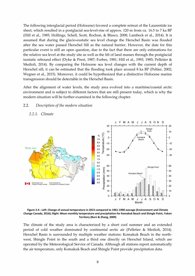
Figure 2-4 - Left: Change of annual temperature in 2015 compared to 1961-1990 average (Environment and Climate Change Canada, 2016); Right: Mean monthly temperature and precipitation for Komakuk Beach and Shingle Point, Yukon

Territory (Burn & Zhang, 2009)

The climate of the study area is characterized by a short cool summer and an extended period of cold weather dominated by continental arctic air (Pelletier & Medioli, 2014). Herschel Basin is surrounded by multiple weather stations: Komakuk Beach in the north-west, Shingle Point in the south and a third one directly on Herschel Island, which are operated by the Meteorological Service of Canada. Although all stations report automatically the air temperature, only Komakuk Beach and Shingle Point provide precipitation data.

10

Burn & Zhang (2009) combined the mean monthly temperature and precipitation for Komakuk Beach and Shingle Point for the period 1971 - 2000 as depicted on the right side of Figure 2-4. On average, the warmest months at all three location do not exceed 15 °C, while in February temperature can reach -30 °C (Burn & Zhang, 2009; Pelletier & Medioli, 2014; Rampton, 1982).

The area is characterized by low annual mean air temperature: -11 °C on Komakuk Beach and -9.9 °C at Shingle Point (1971-2000), whereas Herschel Island has an annual mean temperature of -9.6 °C (1999-2005) (Burn & Zhang, 2009). However the latest temperature data for Herschel Island provided by government of Canada (http://climate.weather.gc.ca) show an increase in annual air temperature to -8.2 °C (2009-2014). This rise coincides with the observation by the Department of Environment (Environment and Climate Change Canada) for the Yukon Territory with an annual air temperature increase of 2.9 °C in 2015 compared to the base line average (1961-1990) as illustrated in Figure 2-4.

The observed average annual precipitation ranges from 254 mm (Shingle Point) to 161 mm (Komakuk Beach)(Burn & Zhang, 2009). Beginning in May, precipitation occurs mainly in form of rain and carries on until November (Pelletier & Medioli, 2014). Additionally, snow melt starts in May, resulting in the highest discharge of rivers in June (Carmack & Macdonald, 2002; Hill, Blasco, Harper, & Fissel, 1991; Reimnitz & Wolf, 1998).

Due to the low summer temperatures as well as low precipitation, the study area can be classified as polar desert or according to the Köppen-Geiger climate classification as polar tundra (Köppen-Geiger code: ET) (Kottek, Grieser, Beck, Rudolf, & Rubel, 2006). The harsh and cold conditions have “a major influence on the distribution of plant communities and individual species” (Pelletier & Medioli, 2014) resulting in a prevalent vegetation with lichens, grasses, mosses, herbs and shrubs (Smith et al., 1989).

2.2.2. Currents and possible inflows

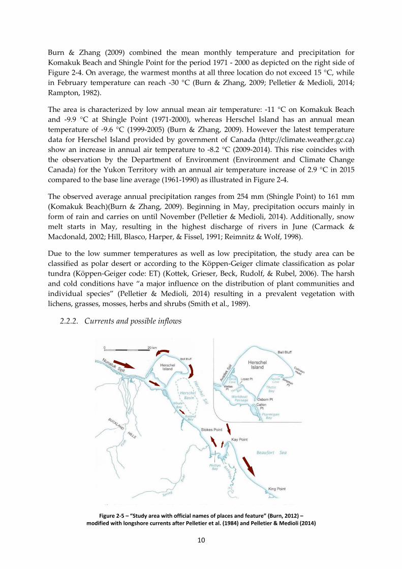
Figure 2-5 – “Study area with official names of places and feature” (Burn, 2012) – modified with longshore currents after Pelletier et al. (1984) and Pelletier & Medioli (2014)

11

The study area is characterized by multiple diverse inflows into the basin with either fluvial or maritime background. There are three tributaries directly entering the basin, which are Babbage River, Spring River and Roland Creek, although they vary in their volumetric extent: (Burn, 2012; Burn & Zhang, 2009; Forbes, 1981; O’Connor, 1984).

In general, the highest flow can be observed for the Babbage River during the months of snow melt, as mentioned in the previous subchapter, which are primarily in May and June. Since the discharge of the snow melt depends on temperature, solar radiation, precipitation and existing snow cover, it is variable from year to year (Carmack & Macdonald, 2002; Cockburn & Lamoureux, 2008; Forbes, 1981; Hill, Lewis, Desmarais, Kauppaymuthoo, & Rais, 2001). For instance, Forbes (1981) observed an annual peak discharge from 1974 to 1977 for the Babbage River between 380 and 580 m³/s, whereas the Meteorological Service of Canada monitored an annual mean flow of 11 m³/s between 1972 and 1994 (Ayles & Snow, 2002).

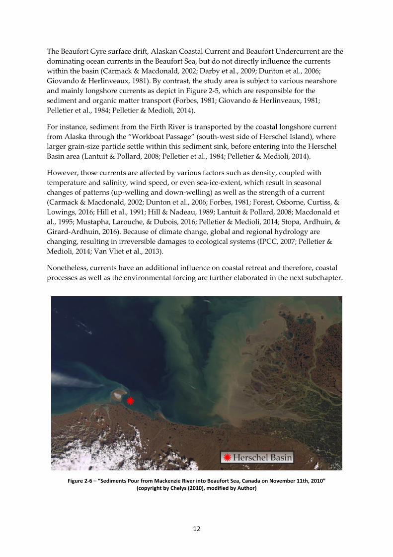
In addition, two rivers potentially influence the contribution of organic matter and sediments into the basin: the Firth River in the northwest and the Mackenzie River/Mackenzie Delta in the southeast of the study area. Their share partially depends on the occurring weather conditions as well as ocean and longshore currents. However, their wide-reaching influence in the distribution of sediment has been proved by multiple studies (Ayles & Snow, 2002; Carmack & Macdonald, 2002; Forbes, 1981; Giovando & Herlinveaux, 1981; Hill et al., 2001; Macdonald et al., 1998; Pelletier et al., 1984) and is also detectable as a visible plume in the immediate vicinity or on satellite images as displayed in Figure 2-6.

The Mackenzie River has a drainage area of 1.68 million km² and an annual mean flow of 8,980 m³/s, compared to Firth River’s annual mean flow of 37.7 m³/s, which makes it the fourth largest river entering the Arctic Ocean (Ayles & Snow, 2002; Macdonald et al., 1998; Macdonald, Paten, & Carmack, 1995). Consequently, the Mackenzie River discharges large portion of sediment, particular and dissolved carbon (POC and DOC, respectively) into the Arctic Ocean and the Canadian Eastern Beaufort Shelf. By comparison, the Firth River emits west of Herschel Island into the Western Beaufort Shelf comparable negligible amounts.

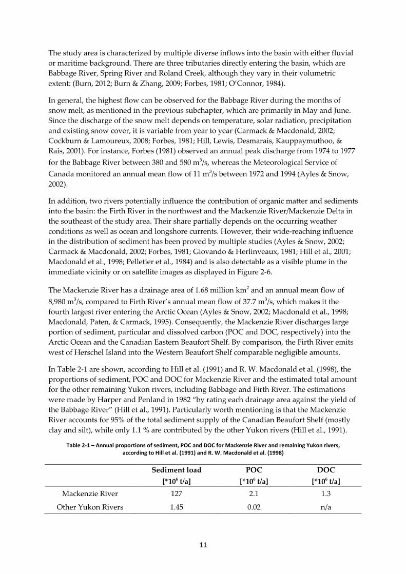
In Table 2-1 are shown, according to Hill et al. (1991) and R. W. Macdonald et al. (1998), the proportions of sediment, POC and DOC for Mackenzie River and the estimated total amount for the other remaining Yukon rivers, including Babbage and Firth River. The estimations were made by Harper and Penland in 1982 “by rating each drainage area against the yield of the Babbage River” (Hill et al., 1991). Particularly worth mentioning is that the Mackenzie River accounts for 95% of the total sediment supply of the Canadian Beaufort Shelf (mostly clay and silt), while only 1.1 % are contributed by the other Yukon rivers (Hill et al., 1991).

Table 2-1 – Annual proportions of sediment, POC and DOC for Mackenzie River and remaining Yukon rivers, according to Hill et al. (1991) and R. W. Macdonald et al. (1998)

Sediment load

[*106 t/a] POC

[*106 t/a] DOC

[*106 t/a] Mackenzie River 127 2.1 1.3

Other Yukon Rivers 1.45 0.02 n/a

12

The Beaufort Gyre surface drift, Alaskan Coastal Current and Beaufort Undercurrent are the dominating ocean currents in the Beaufort Sea, but do not directly influence the currents within the basin (Carmack & Macdonald, 2002; Darby et al., 2009; Dunton et al., 2006; Giovando & Herlinveaux, 1981). By contrast, the study area is subject to various nearshore and mainly longshore currents as depict in Figure 2-5, which are responsible for the sediment and organic matter transport (Forbes, 1981; Giovando & Herlinveaux, 1981; Pelletier et al., 1984; Pelletier & Medioli, 2014).

For instance, sediment from the Firth River is transported by the coastal longshore current from Alaska through the “Workboat Passage” (south-west side of Herschel Island), where larger grain-size particle settle within this sediment sink, before entering into the Herschel Basin area (Lantuit & Pollard, 2008; Pelletier et al., 1984; Pelletier & Medioli, 2014).

However, those currents are affected by various factors such as density, coupled with temperature and salinity, wind speed, or even sea-ice-extent, which result in seasonal changes of patterns (up-welling and down-welling) as well as the strength of a current (Carmack & Macdonald, 2002; Dunton et al., 2006; Forbes, 1981; Forest, Osborne, Curtiss, & Lowings, 2016; Hill et al., 1991; Hill & Nadeau, 1989; Lantuit & Pollard, 2008; Macdonald et al., 1995; Mustapha, Larouche, & Dubois, 2016; Pelletier & Medioli, 2014; Stopa, Ardhuin, & Girard-Ardhuin, 2016). Because of climate change, global and regional hydrology are changing, resulting in irreversible damages to ecological systems (IPCC, 2007; Pelletier & Medioli, 2014; Van Vliet et al., 2013).

Nonetheless, currents have an additional influence on coastal retreat and therefore, coastal processes as well as the environmental forcing are further elaborated in the next subchapter.

Figure 2-6 – “Sediments Pour from Mackenzie River into Beaufort Sea, Canada on November 11th, 2010” (copyright by Chelys (2010), modified by Author)

13

2.2.3. Coastal processes and environmental forcing

As many studies have concluded, not only rivers and currents contribute to the organic carbon and sediment budget, but also the continuously increasing coastal erosion within the study area (Forbes, 2011; Hill et al., 1991; Lantuit, Overduin, et al., 2012; Lantuit & Pollard, 2008; Macdonald et al., 1998; Rachold et al., 2000; Rachold, Are, Atkinson, Cherkashov, & Solomon, 2005). Therefore, it is substantial to understand the dynamics of those coastal processes and the linked environmental forcing.

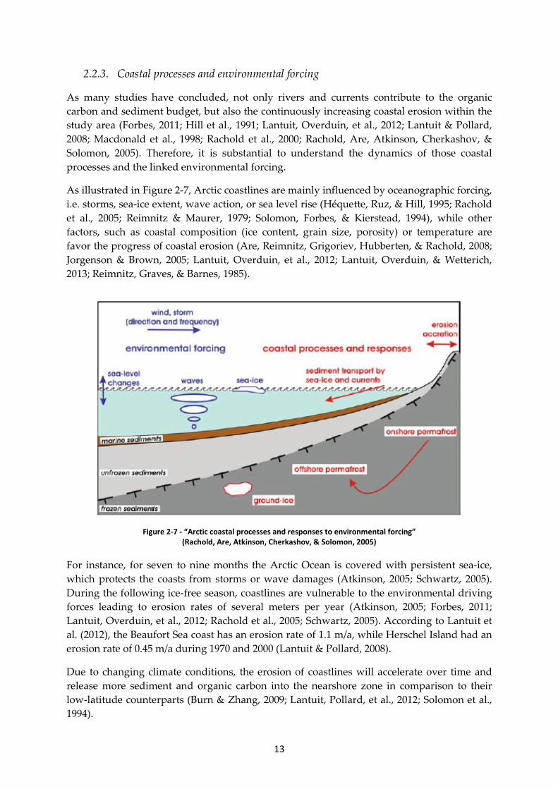
As illustrated in Figure 2-7, Arctic coastlines are mainly influenced by oceanographic forcing, i.e. storms, sea-ice extent, wave action, or sea level rise (Héquette, Ruz, & Hill, 1995; Rachold et al., 2005; Reimnitz & Maurer, 1979; Solomon, Forbes, & Kierstead, 1994), while other factors, such as coastal composition (ice content, grain size, porosity) or temperature are favor the progress of coastal erosion (Are, Reimnitz, Grigoriev, Hubberten, & Rachold, 2008; Jorgenson & Brown, 2005; Lantuit, Overduin, et al., 2012; Lantuit, Overduin, & Wetterich, 2013; Reimnitz, Graves, & Barnes, 1985).

Figure 2-7 - “Arctic coastal processes and responses to environmental forcing” (Rachold, Are, Atkinson, Cherkashov, & Solomon, 2005)

For instance, for seven to nine months the Arctic Ocean is covered with persistent sea-ice, which protects the coasts from storms or wave damages (Atkinson, 2005; Schwartz, 2005). During the following ice-free season, coastlines are vulnerable to the environmental driving forces leading to erosion rates of several meters per year (Atkinson, 2005; Forbes, 2011; Lantuit, Overduin, et al., 2012; Rachold et al., 2005; Schwartz, 2005). According to Lantuit et al. (2012), the Beaufort Sea coast has an erosion rate of 1.1 m/a, while Herschel Island had an erosion rate of 0.45 m/a during 1970 and 2000 (Lantuit & Pollard, 2008).

Due to changing climate conditions, the erosion of coastlines will accelerate over time and release more sediment and organic carbon into the nearshore zone in comparison to their low-latitude counterparts (Burn & Zhang, 2009; Lantuit, Pollard, et al., 2012; Solomon et al., 1994).

14

However, there are going to be spatial and temporal variations, depending on the changing environmental factors. A predicted increase in air temperature, for instance, will lead to a decrease of the summer sea-ice extent, which, by implication, reduces the protection mechanism through sea ice during an extended open water season and allows higher waves to generate over open water (Atkinson, 2005; Couture, 2010, after McGillvray, Agnew, McKay, Pilkington, & Hill, 1993).

Additionally, a simultaneous increase in sea water temperature could support thermal and mechanical erosion, because the frozen coast will be hit by numerous storm surges with warmer water through higher wind speed causing thermal abrasion (Kobayashi, Vidrine, Nairn, & Solomon, 1999; Solomon et al., 1994). Further, it is predicted that due to climate change the sea level will rise, causing larger waves and frequent storms to approach the susceptible coastline (Are et al., 2008; Lambert, 1995; Manson & Solomon, 2007; Schwartz, 2005).

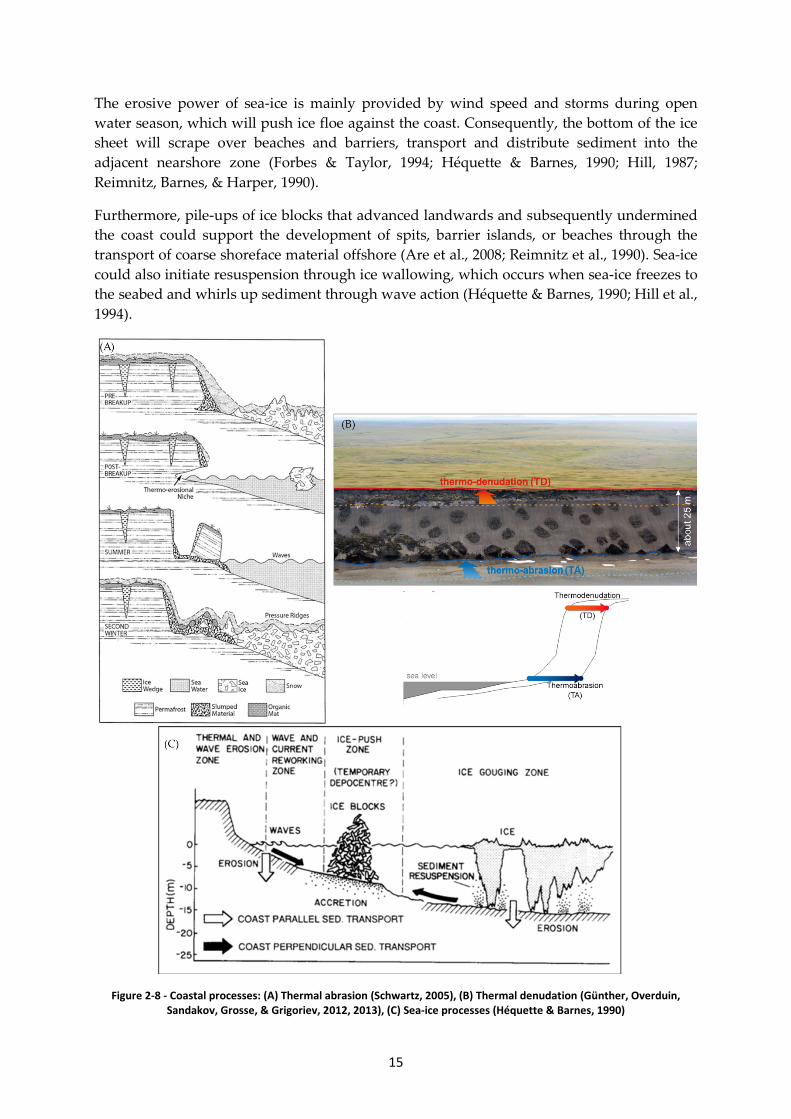
Currently, there are three dominant types of erosion processes that are unique to regions with a colder climate, which includes the study area (Forbes, 2011; Héquette & Barnes, 1990; Lantuit, Overduin, et al., 2012; Lantuit, Pollard, et al., 2012; Lantuit & Pollard, 2008) (see also Figure 2-8):

(1) Thermal abrasion

The first type of erosion processes occurs at coastlines, which are exposed to a combination of thermal and mechanical processes during open water conditions. The sea water causes a rapid melting of the ice-rich sediment through a “convective heat transfer between seawater and the melting surface of the frozen cliff sediment” (Schwartz, 2005). In the meantime, waves are removing unfrozen sediment and continuously undercutting cliffed coasts (mechanical process) (Are, 1988; Kobayashi et al., 1999). As a result, the permafrost coasts are subject to high and rapid coastal retreat and block failure may even occur (Reimnitz et al., 1985; Reimnitz & Maurer, 1979; Ruz, Héquette, & Hill, 1992; Schwartz, 2005). According to MacDonald & Lewis (1973) and Ruz, Héquette, & Hill (1992), the coarser fraction (gravel and sand) will be transported along shore and create beaches and spits nearby, while the finer grained sediment are transported offshore via currents.

(2) Thermo-denudation

Compared to the thermo-abrasion, during thermal denudation only the thermal process is effective. During thermo-denudation process thawing permafrost coasts, which were exposed to the sensible heat flux by water, air, or direct solar radiation, are characterized by a fast retreating headwall and the following downslope-directed transport of excess material (Are, 1988; Günther et al., 2015; Kobayashi et al., 1999; Mudrov, 2007).

(3) Sea-ice processes

The last group of processes is associated with sea-ice, which only temporally influence the face of the shore through abrasion as well as the coastal dynamics and the local sediment budget through the accumulation and transport of sediment into the nearshore zone (Héquette & Barnes, 1990; Hill, 1987; Hill, Barnes, Héquette, & Ruz, 1994; Ogorodov, 2003; Reimnitz et al., 1985).

15

The erosive power of sea-ice is mainly provided by wind speed and storms during open water season, which will push ice floe against the coast. Consequently, the bottom of the ice sheet will scrape over beaches and barriers, transport and distribute sediment into the adjacent nearshore zone (Forbes & Taylor, 1994; Héquette & Barnes, 1990; Hill, 1987; Reimnitz, Barnes, & Harper, 1990).

Furthermore, pile-ups of ice blocks that advanced landwards and subsequently undermined the coast could support the development of spits, barrier islands, or beaches through the transport of coarse shoreface material offshore (Are et al., 2008; Reimnitz et al., 1990). Sea-ice could also initiate resuspension through ice wallowing, which occurs when sea-ice freezes to the seabed and whirls up sediment through wave action (Héquette & Barnes, 1990; Hill et al., 1994).

Figure 2-8 - Coastal processes: (A) Thermal abrasion (Schwartz, 2005), (B) Thermal denudation (Günther, Overduin,

Sandakov, Grosse, & Grigoriev, 2012, 2013), (C) Sea-ice processes (Héquette & Barnes, 1990)

16

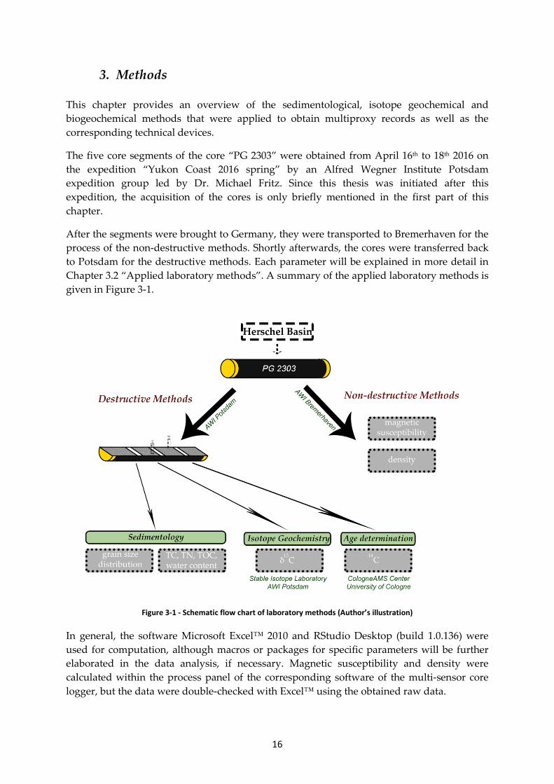
This chapter provides an overview of the sedimentological, isotope geochemical and biogeochemical methods that were applied to obtain multiproxy records as well as the corresponding technical devices.

The five core segments of the core “PG 2303” were obtained from April 16th to 18th 2016 on the expedition “Yukon Coast 2016 spring” by an Alfred Wegner Institute Potsdam expedition group led by Dr. Michael Fritz. Since this thesis was initiated after this expedition, the acquisition of the cores is only briefly mentioned in the first part of this chapter.

After the segments were brought to Germany, they were transported to Bremerhaven for the process of the non-destructive methods. Shortly afterwards, the cores were transferred back to Potsdam for the destructive methods. Each parameter will be explained in more detail in Chapter 3.2 “Applied laboratory methods”. A summary of the applied laboratory methods is given in Figure 3-1.

Figure 3-1 - Schematic flow chart of laboratory methods (Author’s illustration)

In general, the software Microsoft Excel™ 2010 and RStudio Desktop (build 1.0.136) were used for computation, although macros or packages for specific parameters will be further elaborated in the data analysis, if necessary. Magnetic susceptibility and density were calculated within the process panel of the corresponding software of the multi-sensor core logger, but the data were double-checked with Excel™ using the obtained raw data.

3. Methods

17

Equipment 3.1.

The sediment core PG2303 was recovered using a piston corer system by UWITEC and PVC-liner (length: three meter; inner diameter: 60 mm). As illustrated in Figure 3-2 and Figure 3-3, the system consists of a tripod, which is mounted on the sea ice above the targeted sampling site, sampling gadget and three winches that operate the coring process.

Figure 3-2 - Piston corer system used for this expedition (Dr. Boris Biskaborn, AWI, 2016)

Each winch is designated to a specific task:

a. The first winch controls the rope of the metal tube with the PVC-liner. b. The second regulates the release of the piston. c. The third winch is connected to the weight that drives the corer into the sediment.

Figure 3-3 - Sampling gadget and its functionality (U.S. Geological Survey, 2013; UWITEC, 2016)

The sampling procedure starts by fixing the winch with the piston at the target depth. Afterwards, the rope with the weight is released, which hammers the core catcher into the sediment. The procedure ends once the piston reaches the upper end of the tube. During the sampling, water is forced downwards, thereby fixing the sediment in the PVC-liner by sealing the lower end of the corer with a rubber sleeve.

18

The sampling procedure was conducted five times, while each time the entry into the sediment was shifted. After recovery, the five PVC-liners filled with sediments of the overlapping segments were cut in pieces up to 100 cm. Each liner was stored cool - above freezing - until further treatment at the laboratories.

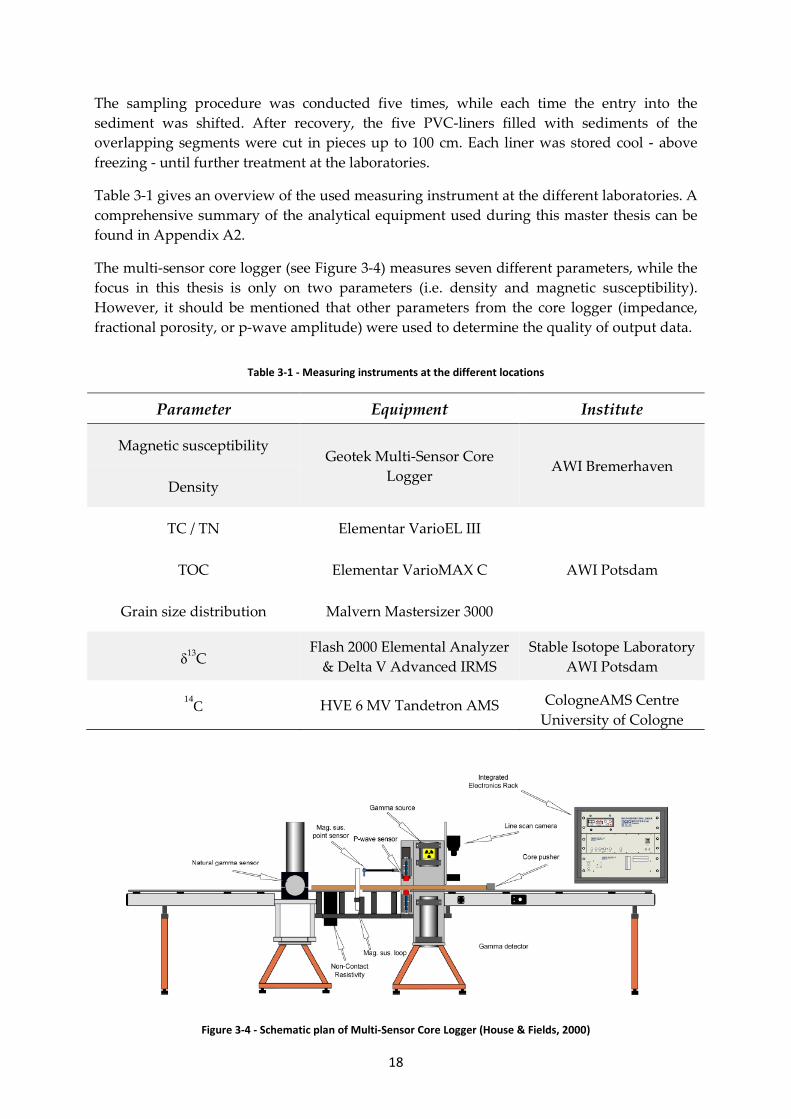
Table 3-1 gives an overview of the used measuring instrument at the different laboratories. A comprehensive summary of the analytical equipment used during this master thesis can be found in Appendix A2.

The multi-sensor core logger (see Figure 3-4) measures seven different parameters, while the focus in this thesis is only on two parameters (i.e. density and magnetic susceptibility). However, it should be mentioned that other parameters from the core logger (impedance, fractional porosity, or p-wave amplitude) were used to determine the quality of output data.

Table 3-1 - Measuring instruments at the different locations

Parameter Equipment Institute

Magnetic susceptibility Geotek Multi-Sensor Core

Logger AWI Bremerhaven

Density

TC / TN Elementar VarioEL III

AWI Potsdam TOC Elementar VarioMAX C

Grain size distribution Malvern Mastersizer 3000

δ13C Flash 2000 Elemental Analyzer

& Delta V Advanced IRMS Stable Isotope Laboratory

AWI Potsdam

14C HVE 6 MV Tandetron AMS

CologneAMS Centre University of Cologne

Figure 3-4 - Schematic plan of Multi-Sensor Core Logger (House & Fields, 2000)

19

Applied laboratory methods 3.2.

The applied laboratory methods for this Master’s thesis will be divided into two subsections: non-destructive and destructive methods. Microbiological activity analyses on the core have been conducted in advance of this work and therefore shall not be discussed further.

3.2.1. Non-destructive methods

After the transfer from the Yukon Territory to the research facility in Potsdam and temporary storage of the core segments there, all sections were transported to Bremerhaven for the non-destructive methods. The experiments took place on August 22nd and August 23rd 2016 at the Alfred-Wegener-Institute headquarters under the supervision of Catalina Gebhardt.

For the analysis the GEOTEK Multi-Sensor Core Logger were used to establish the data of the following parameters:

a) density and

b) magnetic susceptibility.

Following the arrival, the cores were stored at room temperature for a stable further processing. Each core was positioned on a guide rail and pushed by the core pusher in an interval of one centimeter forward into the measuring instruments. To separate the individual cores in the analysis from each other, a hollow cylinder was placed between them. Further on, each parameter is described in detail in the following text.

a. Density

The bulk density of the cores was measured using a gamma ray source and detector (see Figure 3-4). Both devices were mounted at the same height that the center of the core was quantified. As gamma ray source a 10 milli-curie Caesium-137 capsule was used that emits gamma energy around 0.662 MeV. The counterpart is a scintillator (NaI(Tl) crystal with a five cm diameter and five cm thickness) and integral photo-multiplier tube working as a detector controlled through the software and internal microprocessor. The narrow gamma ray beam of the Caesium-137 emits photons, which are scattered by the electrons in the core. By implication, unscattered photons detected by the gamma ray detector can quantify the bulk density of the corresponding core material in g/cm³. (cf. House & Fields, 2000 – chapter 3.3)

According to House & Fields (2000), the following equation was used to determine the bulk density:

ρ = 1/µd * ln (I0/I) (Eq. 1)

where: ρ = sediment bulk density [g/cm³] µ = Compton attenuation coefficient d = sediment thickness I0 = gamma source intensity

I = measured intensity through the sample

20

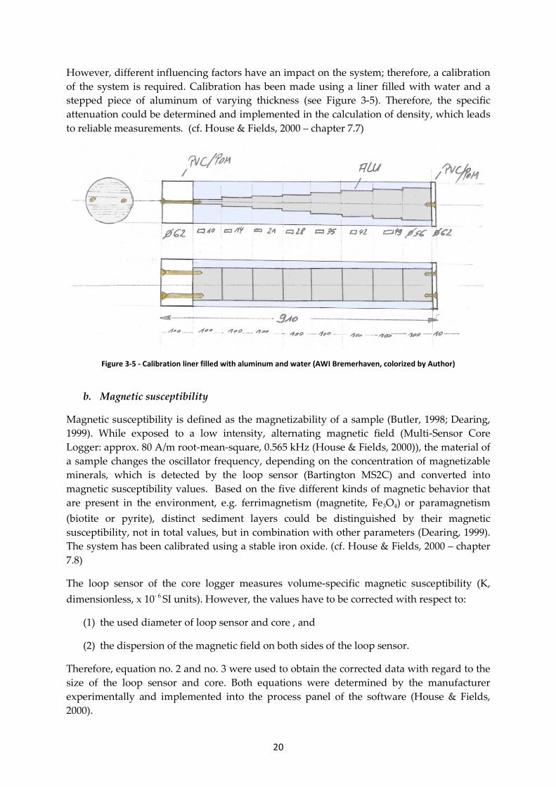
However, different influencing factors have an impact on the system; therefore, a calibration of the system is required. Calibration has been made using a liner filled with water and a stepped piece of aluminum of varying thickness (see Figure 3-5). Therefore, the specific attenuation could be determined and implemented in the calculation of density, which leads to reliable measurements. (cf. House & Fields, 2000 – chapter 7.7)

Figure 3-5 - Calibration liner filled with aluminum and water (AWI Bremerhaven, colorized by Author)

b. Magnetic susceptibility

Magnetic susceptibility is defined as the magnetizability of a sample (Butler, 1998; Dearing, 1999). While exposed to a low intensity, alternating magnetic field (Multi-Sensor Core Logger: approx. 80 A/m root-mean-square, 0.565 kHz (House & Fields, 2000)), the material of a sample changes the oscillator frequency, depending on the concentration of magnetizable minerals, which is detected by the loop sensor (Bartington MS2C) and converted into magnetic susceptibility values. Based on the five different kinds of magnetic behavior that are present in the environment, e.g. ferrimagnetism (magnetite, Fe3O4) or paramagnetism (biotite or pyrite), distinct sediment layers could be distinguished by their magnetic susceptibility, not in total values, but in combination with other parameters (Dearing, 1999). The system has been calibrated using a stable iron oxide. (cf. House & Fields, 2000 – chapter 7.8)

The loop sensor of the core logger measures volume-specific magnetic susceptibility (K, dimensionless, x 10- 6 SI units). However, the values have to be corrected with respect to:

(1) the used diameter of loop sensor and core , and

(2) the dispersion of the magnetic field on both sides of the loop sensor.

Therefore, equation no. 2 and no. 3 were used to obtain the corrected data with regard to the size of the loop sensor and core. Both equations were determined by the manufacturer experimentally and implemented into the process panel of the software (House & Fields, 2000).

21

K = Kuncor / Krel (Eq. 2)

Krel = 4.8566*(d/Dl)² - 3.0163(d/Dl) – 0.6448 (Eq. 3)

where: K = volume-specific magnetic susceptibility [*10- 6 SI unit] Kuncor = uncorrected values Krel = diameter-considered values d = core diameter [60 mm] Dl = loop diameter [80 mm]

The second problem with the momentum of the magnetic field was overcome by using Excel™. Starting at 5 cm apart from the point of attachment of hollow cylinder and core segment, the corresponding values were summed and divided by two. This procedure was done for the remaining four centimeters as illustrated in Figure 3-6.

Figure 3-6 - Solving the issue by the momentum of the magnetic field (Author's illustration)

As final step, the volume susceptibility was converted into the mass-specific magnetic susceptibility by using the following equation (Butler, 1998; Dearing, 1999; House & Fields, 2000):

χ = K / ρ (Eq. 4)

where: χ = mass-specific magnetic susceptibility [*10- 9 m³/kg] K = volume-specific magnetic susceptibility [*10- 6 SI unit] ρ = sediment bulk density [g/cm³]

The sediment bulk density was established from the gamma ray density measurement as mentioned in chapter 3.2.1 a). In comparison to the volume magnetic susceptibility, the mass-specific magnetic susceptibility will take into account the occurrence of compressed and denser material at lower segment of the drilling core and therefore, expresses a higher significance of the material itself.

22

3.2.2. Destructive methods

After successfully acquiring the needed data from the non-destructive methods, the destructive analysis of the drilling core could be realized. All segments were transferred back to Potsdam and the preparation and processing of samples took place from September 22nd to December 8th 2016, except for the external measurement of the δ13C determination and 14C dating. The destructive methods included elementary (TC/TN/TOC), δ13C and grain size analyses and 14C dating, which will be further described in this chapter.

Firstly, all cores were separated into two halves: one archive half and one working half. After smoothing the surface, taking pictures and describing the visual condition of the core, samples were taken every ten centimeters on the working half with a syringe or a scraper and placed into 12.5 ml plastic jars. The samples for grain size analysis are shifted by one centimeter in comparison to the other samples, due to material management. Overall, for this thesis 131 samples were taken for elementary analysis as well as 25 samples for grain size analysis and eight hand-picked macrofossils for 14C dating.

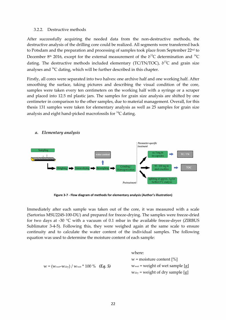
a. Elementary analysis

Figure 3-7 - Flow diagram of methods for elementary analysis (Author’s illustration)

Immediately after each sample was taken out of the core, it was measured with a scale (Sartorius MSU224S-100-DU) and prepared for freeze-drying. The samples were freeze-dried for two days at -30 °C with a vacuum of 0.1 mbar in the available freeze-dryer (ZIRBUS Sublimator 3-4-5). Following this, they were weighed again at the same scale to ensure continuity and to calculate the water content of the individual samples. The following equation was used to determine the moisture content of each sample:

w = (wwet-wdry) / wwet * 100 % (Eq. 5)

where: w = moisture content [%] wwet = weight of wet sample [g] wdry = weight of dry sample [g]

23

The next step was to grind and homogenize the samples by using a planetary mill (Fritsch Pulverisette 5), which was equipped with agate jars that were filled with three agate balls and one sample per jar. After eight minutes at 360 rpm, the samples were transferred back into the 12.5 ml plastic jars using a soft brush and a spatula. Additionally, approximately one gram of each sample was deducted for further δ13C analysis.

Information about the contents of total nitrogen (TN), total carbon (TC) and total organic carbon (TOC) can be utilized to reconstruct paleoenvironmental conditions. The main reason for this assertion is given by the genesis of marine sediment. Besides the accumulation of transported sediments from different locations, it is also a depositional location for past biota (Meyers, 1997; Meyers & Lallier-Vergès, 1999). Therefore, information about the environmental condition during the decay and accumulation of organic substances as well as the bioproductivity can be gained using the biogeochemical parameters. This is due to the fact that the residual contents of carbon and nitrogen within the sediment were subject to specific environmental factors (e.g. temperature or pH) during and before their deposition.

For quantifying the amount of TN and TC about 5 mg were encapsulated into tin capsules on a Sartorius micro M3P scale, twice for each sample, in combination with a small amount of tungsten (VI) oxide to catalyze the combustion of the soil sample. Immediately after this, the sediment samples, blank capsules as well as control standards and calibration (see Table 3-2) were measured quantitatively using the CN elementary analyzer (Elementar varioEL III, Elementar Analysensysteme GmbH, 2002) at the research facility in Potsdam.

Table 3-2 - Standards and calibration samples for TC and TN measurement

Substance C/N-content Calibration / Control Sample Nicotinamide (2x) C = 59 % N = 22.9 %

Calibration (only once per measuring day) EDTA 20% (4x) C = 20 % N = 4.67 %

EDTA 10:40 (4x) C = 8.22 % N = 1.918 % IVA 2176 (soil standard) C = 15.95 % N = 1.29 %

Control group (each time after 15 samples)

CaCO3 12% C = 12 % N = 0 % IVA 2150 (soil standard) C = 6.44 % N = 0.49 %

Soil standard 1 C = 3.5 % N = 0.216 % Soil standard 4 C = 2.417 % N = 0.048 % Soil standard 2 C = 0.732 % N = 0.064 %

The measurements are based on the principle of a combustion process at 950 °C, where in an high oxygen-saturated helium atmosphere the elements of a sample (C, H, N and S) are explosively oxidized into their gaseous phases (CO₂, H₂O, NOx, SO₂, SO₃) and molecular N₂ (Elementar Analysensysteme GmbH, 2002). Thereby, a tube filled with elemental copper serves as a catalyst for the reduction of nitrous oxide (NOx) to N₂ at a temperature of 500 °C. Furthermore, SO₂ and SO₃ are adsorbed by Cer-VI-oxid, which is why sulfur is not measured for those samples. Afterward, the remaining gases are transported via the helium atmosphere to the measuring chamber for the detection of thermal conductivity of each gas. The resulting peaks were transmitted to the accompanying software and calculated as percentage share of carbon and nitrogen in comparison to the input sample weight. The detection limit of the measurement was 0.1 % for nitrogen and 0.05 % for carbon.

24

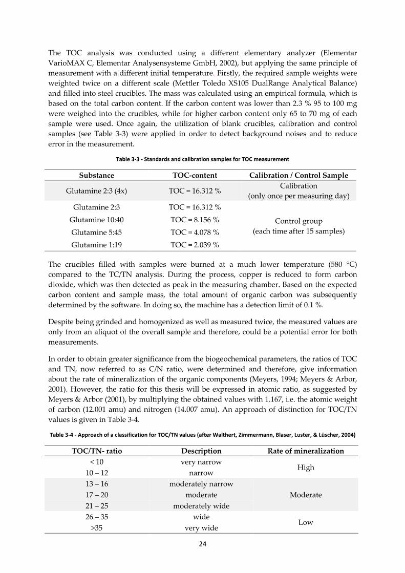
The TOC analysis was conducted using a different elementary analyzer (Elementar VarioMAX C, Elementar Analysensysteme GmbH, 2002), but applying the same principle of measurement with a different initial temperature. Firstly, the required sample weights were weighted twice on a different scale (Mettler Toledo XS105 DualRange Analytical Balance) and filled into steel crucibles. The mass was calculated using an empirical formula, which is based on the total carbon content. If the carbon content was lower than 2.3 % 95 to 100 mg were weighed into the crucibles, while for higher carbon content only 65 to 70 mg of each sample were used. Once again, the utilization of blank crucibles, calibration and control samples (see Table 3-3) were applied in order to detect background noises and to reduce error in the measurement.

Table 3-3 - Standards and calibration samples for TOC measurement

Substance TOC-content Calibration / Control Sample

Glutamine 2:3 (4x) TOC = 16.312 % Calibration

(only once per measuring day) Glutamine 2:3 TOC = 16.312 %

Control group (each time after 15 samples)

Glutamine 10:40 TOC = 8.156 % Glutamine 5:45 TOC = 4.078 % Glutamine 1:19 TOC = 2.039 %

The crucibles filled with samples were burned at a much lower temperature (580 °C) compared to the TC/TN analysis. During the process, copper is reduced to form carbon dioxide, which was then detected as peak in the measuring chamber. Based on the expected carbon content and sample mass, the total amount of organic carbon was subsequently determined by the software. In doing so, the machine has a detection limit of 0.1 %.

Despite being grinded and homogenized as well as measured twice, the measured values are only from an aliquot of the overall sample and therefore, could be a potential error for both measurements.

In order to obtain greater significance from the biogeochemical parameters, the ratios of TOC and TN, now referred to as C/N ratio, were determined and therefore, give information about the rate of mineralization of the organic components (Meyers, 1994; Meyers & Arbor, 2001). However, the ratio for this thesis will be expressed in atomic ratio, as suggested by Meyers & Arbor (2001), by multiplying the obtained values with 1.167, i.e. the atomic weight of carbon (12.001 amu) and nitrogen (14.007 amu). An approach of distinction for TOC/TN values is given in Table 3-4.

Table 3-4 - Approach of a classification for TOC/TN values (after Walthert, Zimmermann, Blaser, Luster, & Lüscher, 2004)

TOC/TN- ratio Description Rate of mineralization < 10 very narrow

High 10 – 12 narrow 13 – 16 moderately narrow

Moderate 17 – 20 moderate 21 – 25 moderately wide 26 – 35 wide

Low >35 very wide

25

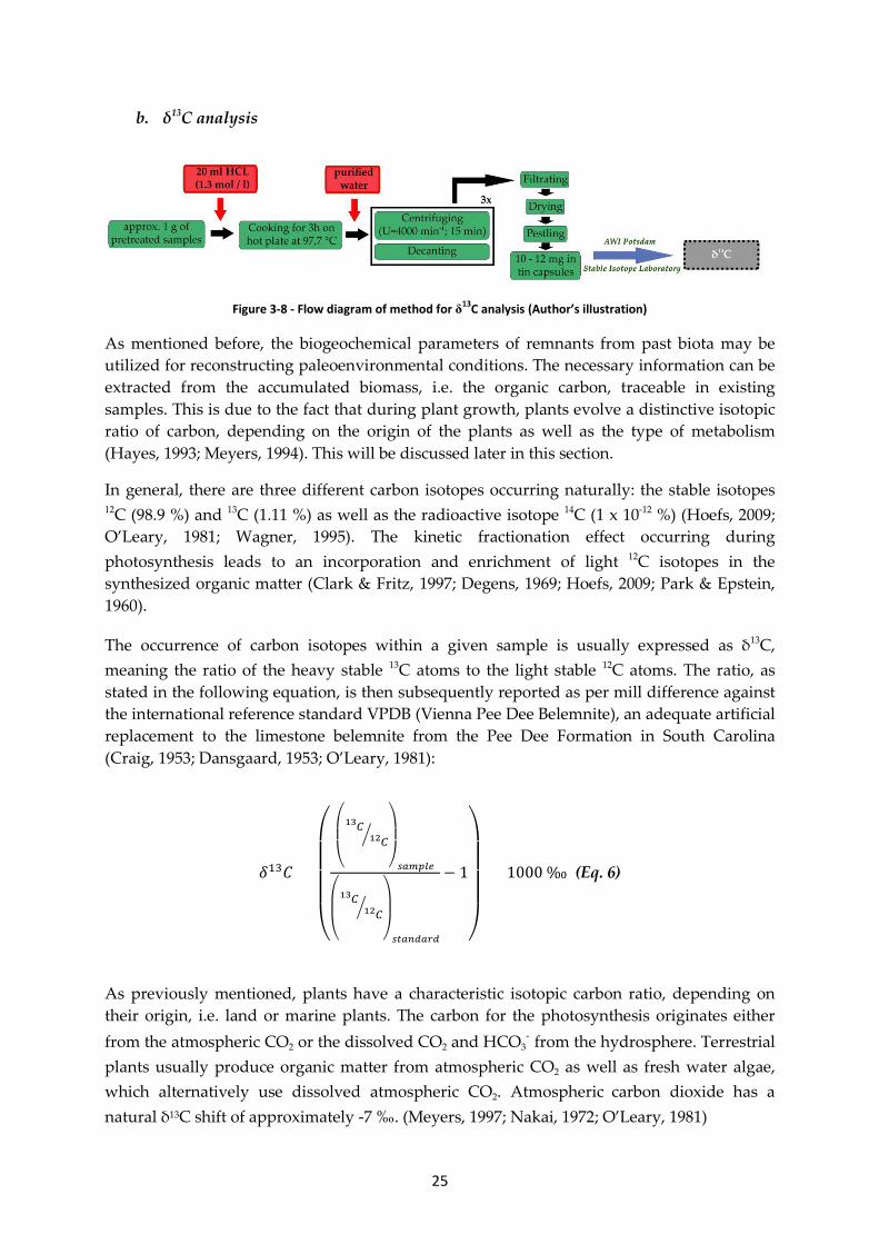
b. δ13C analysis

Figure 3-8 - Flow diagram of method for δ13C analysis (Author’s illustration)

As mentioned before, the biogeochemical parameters of remnants from past biota may be utilized for reconstructing paleoenvironmental conditions. The necessary information can be extracted from the accumulated biomass, i.e. the organic carbon, traceable in existing samples. This is due to the fact that during plant growth, plants evolve a distinctive isotopic ratio of carbon, depending on the origin of the plants as well as the type of metabolism (Hayes, 1993; Meyers, 1994). This will be discussed later in this section.

In general, there are three different carbon isotopes occurring naturally: the stable isotopes 12C (98.9 %) and 13C (1.11 %) as well as the radioactive isotope 14C (1 x 10-12 %) (Hoefs, 2009; O’Leary, 1981; Wagner, 1995). The kinetic fractionation effect occurring during photosynthesis leads to an incorporation and enrichment of light 12C isotopes in the synthesized organic matter (Clark & Fritz, 1997; Degens, 1969; Hoefs, 2009; Park & Epstein, 1960).

The occurrence of carbon isotopes within a given sample is usually expressed as δ13C, meaning the ratio of the heavy stable 13C atoms to the light stable 12C atoms. The ratio, as stated in the following equation, is then subsequently reported as per mill difference against the international reference standard VPDB (Vienna Pee Dee Belemnite), an adequate artificial replacement to the limestone belemnite from the Pee Dee Formation in South Carolina (Craig, 1953; Dansgaard, 1953; O’Leary, 1981):

𝛿13𝐶 =

⎝

⎜⎜⎜⎜⎛

⎝

⎜⎛ 𝐶13

𝐶12�

⎠

⎟⎞

𝑠𝑠𝑠𝑠𝑠𝑠

⎝

⎜⎛ 𝐶13

𝐶12�

⎠

⎟⎞

𝑠𝑠𝑠𝑠𝑠𝑠𝑠𝑠

− 1

⎠

⎟⎟⎟⎟⎞

× 1000 ‰ (Eq. 6)

As previously mentioned, plants have a characteristic isotopic carbon ratio, depending on their origin, i.e. land or marine plants. The carbon for the photosynthesis originates either from the atmospheric CO2 or the dissolved CO2 and HCO3

- from the hydrosphere. Terrestrial plants usually produce organic matter from atmospheric CO2 as well as fresh water algae, which alternatively use dissolved atmospheric CO2. Atmospheric carbon dioxide has a natural δ13C shift of approximately -7 ‰. (Meyers, 1997; Nakai, 1972; O’Leary, 1981)

26

Contrary to this, when dissolved CO2 is only available to a limited extent, the source

switches to bicarbonate (HCO3-), which happens mostly for marine algae. However,

bicarbonate has a weaker ratio, with δ13C values of equal to -1 ‰ (Meyers, 1997; Meyers & Lallier-Vergès, 1999; O’Leary, 1981). Additionally, the corresponding metabolism of the individual plants has a further important role in determining the origin of the sample.

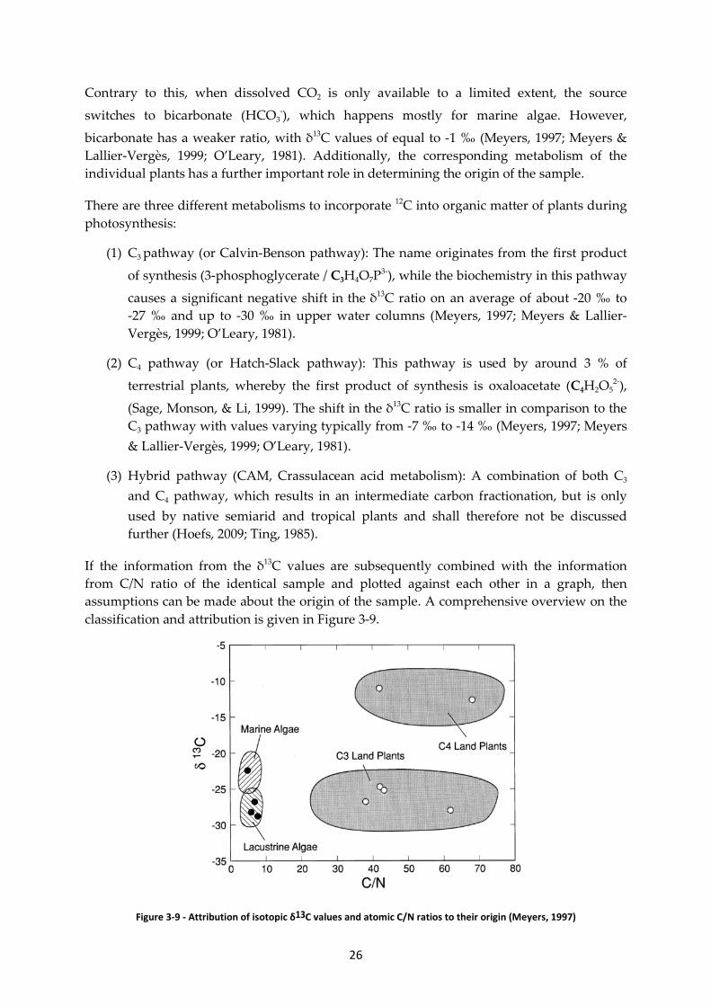
There are three different metabolisms to incorporate 12C into organic matter of plants during photosynthesis:

(1) C3 pathway (or Calvin-Benson pathway): The name originates from the first product

of synthesis (3-phosphoglycerate / C3H4O7P3-), while the biochemistry in this pathway

causes a significant negative shift in the δ13C ratio on an average of about -20 ‰ to -27 ‰ and up to -30 ‰ in upper water columns (Meyers, 1997; Meyers & Lallier-Vergès, 1999; O’Leary, 1981).

(2) C4 pathway (or Hatch-Slack pathway): This pathway is used by around 3 % of

terrestrial plants, whereby the first product of synthesis is oxaloacetate (C4H2O52-),

(Sage, Monson, & Li, 1999). The shift in the δ13C ratio is smaller in comparison to the C3 pathway with values varying typically from -7 ‰ to -14 ‰ (Meyers, 1997; Meyers & Lallier-Vergès, 1999; O’Leary, 1981).

(3) Hybrid pathway (CAM, Crassulacean acid metabolism): A combination of both C3 and C4 pathway, which results in an intermediate carbon fractionation, but is only used by native semiarid and tropical plants and shall therefore not be discussed further (Hoefs, 2009; Ting, 1985).

If the information from the δ13C values are subsequently combined with the information from C/N ratio of the identical sample and plotted against each other in a graph, then assumptions can be made about the origin of the sample. A comprehensive overview on the classification and attribution is given in Figure 3-9.

Figure 3-9 - Attribution of isotopic δ13C values and atomic C/N ratios to their origin (Meyers, 1997)

27

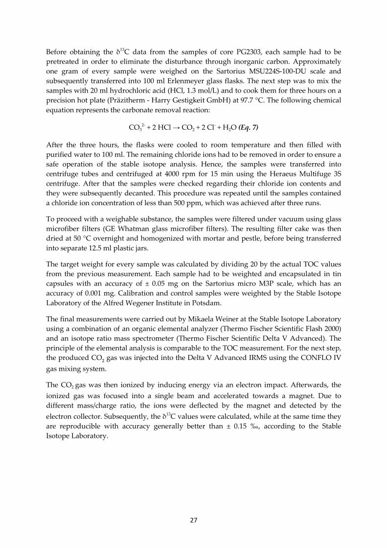
Before obtaining the δ13C data from the samples of core PG2303, each sample had to be pretreated in order to eliminate the disturbance through inorganic carbon. Approximately one gram of every sample were weighed on the Sartorius MSU224S-100-DU scale and subsequently transferred into 100 ml Erlenmeyer glass flasks. The next step was to mix the samples with 20 ml hydrochloric acid (HCl, 1.3 mol/L) and to cook them for three hours on a precision hot plate (Präzitherm - Harry Gestigkeit GmbH) at 97.7 °C. The following chemical equation represents the carbonate removal reaction:

CO32- + 2 HCl → CO2 + 2 Cl- + H2O (Eq. 7)

After the three hours, the flasks were cooled to room temperature and then filled with purified water to 100 ml. The remaining chloride ions had to be removed in order to ensure a safe operation of the stable isotope analysis. Hence, the samples were transferred into centrifuge tubes and centrifuged at 4000 rpm for 15 min using the Heraeus Multifuge 3S centrifuge. After that the samples were checked regarding their chloride ion contents and they were subsequently decanted. This procedure was repeated until the samples contained a chloride ion concentration of less than 500 ppm, which was achieved after three runs.

To proceed with a weighable substance, the samples were filtered under vacuum using glass microfiber filters (GE Whatman glass microfiber filters). The resulting filter cake was then dried at 50 °C overnight and homogenized with mortar and pestle, before being transferred into separate 12.5 ml plastic jars.

The target weight for every sample was calculated by dividing 20 by the actual TOC values from the previous measurement. Each sample had to be weighted and encapsulated in tin capsules with an accuracy of ± 0.05 mg on the Sartorius micro M3P scale, which has an accuracy of 0.001 mg. Calibration and control samples were weighted by the Stable Isotope Laboratory of the Alfred Wegener Institute in Potsdam.

The final measurements were carried out by Mikaela Weiner at the Stable Isotope Laboratory using a combination of an organic elemental analyzer (Thermo Fischer Scientific Flash 2000) and an isotope ratio mass spectrometer (Thermo Fischer Scientific Delta V Advanced). The principle of the elemental analysis is comparable to the TOC measurement. For the next step, the produced CO₂ gas was injected into the Delta V Advanced IRMS using the CONFLO IV gas mixing system.

The CO2 gas was then ionized by inducing energy via an electron impact. Afterwards, the ionized gas was focused into a single beam and accelerated towards a magnet. Due to different mass/charge ratio, the ions were deflected by the magnet and detected by the electron collector. Subsequently, the δ13C values were calculated, while at the same time they are reproducible with accuracy generally better than ± 0.15 ‰, according to the Stable Isotope Laboratory.

28

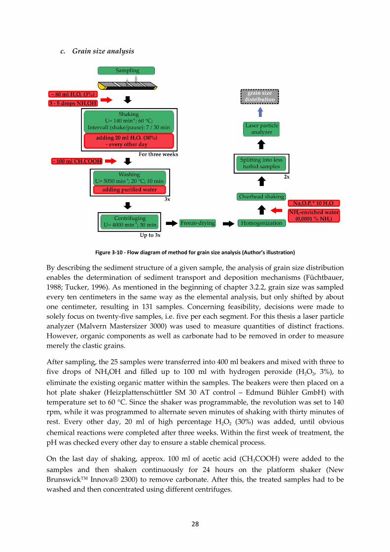
c. Grain size analysis

Figure 3-10 - Flow diagram of method for grain size analysis (Author’s illustration)

By describing the sediment structure of a given sample, the analysis of grain size distribution enables the determination of sediment transport and deposition mechanisms (Füchtbauer, 1988; Tucker, 1996). As mentioned in the beginning of chapter 3.2.2, grain size was sampled every ten centimeters in the same way as the elemental analysis, but only shifted by about one centimeter, resulting in 131 samples. Concerning feasibility, decisions were made to solely focus on twenty-five samples, i.e. five per each segment. For this thesis a laser particle analyzer (Malvern Mastersizer 3000) was used to measure quantities of distinct fractions. However, organic components as well as carbonate had to be removed in order to measure merely the clastic grains.

After sampling, the 25 samples were transferred into 400 ml beakers and mixed with three to five drops of NH4OH and filled up to 100 ml with hydrogen peroxide (H2O2, 3%), to eliminate the existing organic matter within the samples. The beakers were then placed on a hot plate shaker (Heizplattenschüttler SM 30 AT control – Edmund Bühler GmbH) with temperature set to 60 °C. Since the shaker was programmable, the revolution was set to 140 rpm, while it was programmed to alternate seven minutes of shaking with thirty minutes of rest. Every other day, 20 ml of high percentage H2O2 (30%) was added, until obvious chemical reactions were completed after three weeks. Within the first week of treatment, the pH was checked every other day to ensure a stable chemical process.

On the last day of shaking, approx. 100 ml of acetic acid (CH3COOH) were added to the samples and then shaken continuously for 24 hours on the platform shaker (New Brunswick™ Innova® 2300) to remove carbonate. After this, the treated samples had to be washed and then concentrated using different centrifuges.

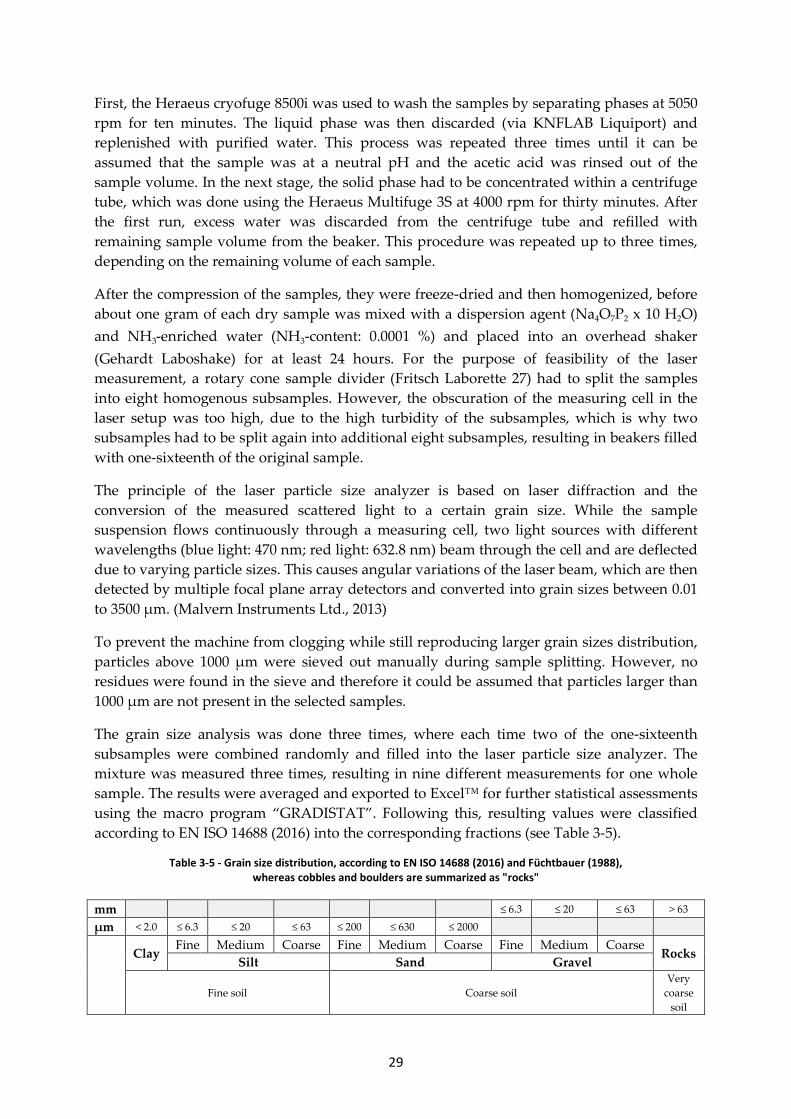
29

First, the Heraeus cryofuge 8500i was used to wash the samples by separating phases at 5050 rpm for ten minutes. The liquid phase was then discarded (via KNFLAB Liquiport) and replenished with purified water. This process was repeated three times until it can be assumed that the sample was at a neutral pH and the acetic acid was rinsed out of the sample volume. In the next stage, the solid phase had to be concentrated within a centrifuge tube, which was done using the Heraeus Multifuge 3S at 4000 rpm for thirty minutes. After the first run, excess water was discarded from the centrifuge tube and refilled with remaining sample volume from the beaker. This procedure was repeated up to three times, depending on the remaining volume of each sample.

After the compression of the samples, they were freeze-dried and then homogenized, before about one gram of each dry sample was mixed with a dispersion agent (Na4O7P2 x 10 H2O) and NH3-enriched water (NH3-content: 0.0001 %) and placed into an overhead shaker (Gehardt Laboshake) for at least 24 hours. For the purpose of feasibility of the laser measurement, a rotary cone sample divider (Fritsch Laborette 27) had to split the samples into eight homogenous subsamples. However, the obscuration of the measuring cell in the laser setup was too high, due to the high turbidity of the subsamples, which is why two subsamples had to be split again into additional eight subsamples, resulting in beakers filled with one-sixteenth of the original sample.

The principle of the laser particle size analyzer is based on laser diffraction and the conversion of the measured scattered light to a certain grain size. While the sample suspension flows continuously through a measuring cell, two light sources with different wavelengths (blue light: 470 nm; red light: 632.8 nm) beam through the cell and are deflected due to varying particle sizes. This causes angular variations of the laser beam, which are then detected by multiple focal plane array detectors and converted into grain sizes between 0.01 to 3500 µm. (Malvern Instruments Ltd., 2013)

To prevent the machine from clogging while still reproducing larger grain sizes distribution, particles above 1000 µm were sieved out manually during sample splitting. However, no residues were found in the sieve and therefore it could be assumed that particles larger than 1000 µm are not present in the selected samples.

The grain size analysis was done three times, where each time two of the one-sixteenth subsamples were combined randomly and filled into the laser particle size analyzer. The mixture was measured three times, resulting in nine different measurements for one whole sample. The results were averaged and exported to Excel™ for further statistical assessments using the macro program “GRADISTAT”. Following this, resulting values were classified according to EN ISO 14688 (2016) into the corresponding fractions (see Table 3-5).

Table 3-5 - Grain size distribution, according to EN ISO 14688 (2016) and Füchtbauer (1988), whereas cobbles and boulders are summarized as "rocks"

mm ≤ 6.3 ≤ 20 ≤ 63 > 63

µm < 2.0 ≤ 6.3 ≤ 20 ≤ 63 ≤ 200 ≤ 630 ≤ 2000

Clay Fine Medium Coarse Fine Medium Coarse Fine Medium Coarse

Rocks Silt Sand Gravel

Fine soil Coarse soil Very

coarse soil

30

d. 14C dating

The dating of organic remains within given sediment samples is essential for the chronological classification of a sediment core and provides evidence about the minimum point in time that the deposition of corresponding layer took place (Ahnert, 1999). Furthermore, assumptions could be made about the average sedimentation rate through the correlation of age determination and sediment depth / thickness, if the organic matter is autochthonous and was not relocated.

The age determination for this thesis was realized using the decay of the radioactive carbon isotope 14C. The 14C isotope is produced permanently by the reaction of the stable nitrogen isotope (14N) with solar neutrons in the upper atmosphere, according to the following equation (Clark & Fritz, 1997):

𝑁714 + 𝑛01 → 𝐶614 + 𝐻11 (Eq. 8)

In the presence of oxygen, carbon 14C is rapidly oxidized to 14CO2 and added to the global

carbon cycle, along with 13CO2 and the most abundant 12CO2 (Wigley & Schimmel, 2000).

During photosynthetic processes, 14CO2 gets incorporated into the biomass and due to the fact that living organisms are in equilibrium with the atmosphere, they hold the same isotopic ratio of radioactive 14C to the stable 12C isotopes (Björck & Wohlfarth, 2001).

With the death of the organism collapses the metabolism and no further nuclides can get incorporated into the organic matter. Meanwhile, the radioactive 14C nuclides decay constantly to 14N with a half-life time of 5,730 ± 40 a (Clark & Fritz, 1997; Engelkemeir, Hamill, Inghram, & Libby, 1949). Therefore, the corresponding radiocarbon age, i.e. the period of time since death of the organism, can be calculated, according to equation no. 9 and no. 10 (Libby, 1955, 1961; Stuiver & Polach, 1977):

𝑡 = 1𝜆∗ ln 𝐶 𝑠=014

𝐶 𝑠=114 (Eq. 9)

𝜆 = ln 2𝑡1/2

(Eq. 10)

where: t = calculated radiocarbon age [a BP] λ = decay constant [a-1] 14Ct=0 = original 14C content [pMC] 14Ct=1 = 14C content after certain time span [pMC]

t1/2 = half-life time of 14C = 5,730 ± 40 a [a]

Usually, the calculated radiocarbon ages are reported in years Before Present (BP) with 1950 AD as the base year, while 14C content is expressed as pMC (percent modern carbon). Due to variations in the global 14C concentration over time, the results have to be calibrated with respect to their location, resulting in a conversion to calendar years (cal BP). Decisions have been made to use the Marine13 radiocarbon age calibration curves for sediment in the range of 0 to 50,000 yr cal BP (Reimer et al., 2013). Despite technical improvements, the only limitation for the atomic mass spectrometry analysis is that a good quality of dating is limited to 40,000 or even 50,000 years BC (Björck & Wohlfarth, 2001; Wagner, 1995). However, this should not be a concern for this thesis, since the target time span was sought under this limit.

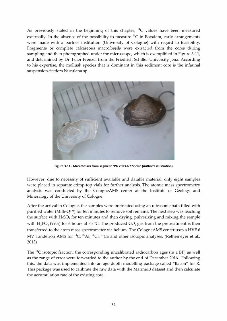
31

As previously stated in the beginning of this chapter, 14C values have been measured externally. In the absence of the possibility to measure 14C in Potsdam, early arrangements were made with a partner institution (University of Cologne) with regard to feasibility. Fragments or complete calcareous macrofossils were extracted from the cores during sampling and then photographed under the microscope, which is exemplified in Figure 3-11, and determined by Dr. Peter Frenzel from the Friedrich Schiller University Jena. According to his expertise, the mollusk species that is dominant in this sediment core is the infaunal suspension-feeders Nuculana sp.

Figure 3-11 - Macrofossils from segment “PG 2303-6 277 cm” (Author’s illustration)

However, due to necessity of sufficient available and datable material, only eight samples were placed in separate crimp-top vials for further analysis. The atomic mass spectrometry analysis was conducted by the CologneAMS center at the Institute of Geology and Mineralogy of the University of Cologne.

After the arrival in Cologne, the samples were pretreated using an ultrasonic bath filled with purified water (Milli-Q™) for ten minutes to remove soil remains. The next step was leaching the surface with H2SO4 for ten minutes and then drying, pulverizing and mixing the sample with H3PO4 (99%) for 6 hours at 75 °C. The produced CO2 gas from the pretreatment is then transferred to the atom mass spectrometer via helium. The CologneAMS center uses a HVE 6 MV Tandetron AMS for 14C, 26Al, 36Cl, 41Ca and other isotopic analyses. (Rethemeyer et al., 2013)

The 14C isotopic fraction, the corresponding uncalibrated radiocarbon ages (in a BP) as well as the range of error were forwarded to the author by the end of December 2016. Following this, the data was implemented into an age-depth modelling package called “Bacon” for R. This package was used to calibrate the raw data with the Marine13 dataset and then calculate the accumulation rate of the existing core.

32

The following chapter comprises the results from the laboratory methods mentioned in the previous chapter. Each outcome will be described in detail in an individual subchapter. Since the mass-specific magnetic susceptibility is based primarily on density and volume-specific magnetic susceptibility, density is represented within the results and will not be discussed further. A summary of all results is given in the Appendix A3.

Visual condition 4.1.

After each core was separated into two halves, the visual condition of the halves was checked. All cores had a brown-grayish to grayish-black tint and were occasionally interrupted by fine fissures and gas cavities, which is exemplified in Figure 4-1 and with a higher resolution picture in Appendix A4. Black organic-rich inclusions were found over multiple centimeters, but were rarely spread over the whole core. A distinctive transition between possible layers was not detectable visually. This could be seen as the first indicator for the grain size analysis that the variation of grain size along the length will change marginally.

Figure 4-1 - Photograph of segment PG 2303-6 (100 – 200 cm) (Author’s illustration)

Magnetic susceptibility 4.2.

During the planning of this Master’s thesis, the data from the calculation of mass-specific magnetic susceptibility were assigned to an additional purpose. Since core “PG 2303” consists of five individual core segments, they had to be fitted in order to represent the entire core. The development of a cumulative core depth through susceptibility was realized by first overlapping the graphs of each adjacent segment visually and then secondly, searching the data for a specific pattern. Afterwards, every segment was cut at a determined point -either the highest or lowest point within the pattern, where values were broadly similar - and connected to a continuous depth. This resulted in a new cumulative core depth of 12.3 m, which we refer to as “depth” in centimeters.

The values of mass-specific magnetic susceptibility over the length are given in Figure 4-2. Due to recommendations by Catalina Gebhardt, density was cross-checked with the data measured by the multi-sensor core logger for p-wave velocity, impedance and fractional porosity and removed, if values were implausible. Furthermore, data were removed for end sections of the cores, since the measurement for those sections were inconsistent.

In general, magnetic susceptibility ranged from 11 to 13 x 10-9 m³/kg, whereas lower values occur in depth from 50 to 250 cm, reaching to 9 x 10-9 m³/kg.

4. Data analysis

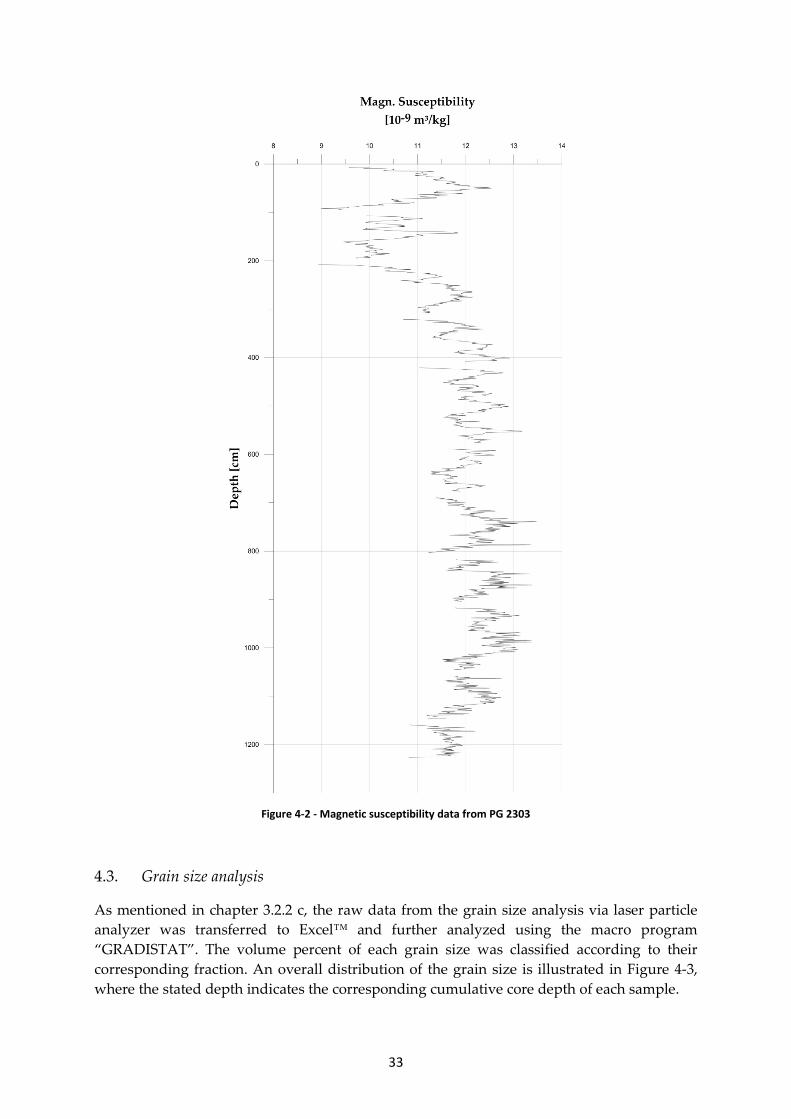
33

Figure 4-2 - Magnetic susceptibility data from PG 2303

Grain size analysis 4.3.

As mentioned in chapter 3.2.2 c, the raw data from the grain size analysis via laser particle analyzer was transferred to Excel™ and further analyzed using the macro program “GRADISTAT”. The volume percent of each grain size was classified according to their corresponding fraction. An overall distribution of the grain size is illustrated in Figure 4-3, where the stated depth indicates the corresponding cumulative core depth of each sample.

34

Figure 4-3 - Grain size distribution of PG 2303

The graphic shows a significant change of grain size distribution from a tapered graph in the upper segment of the core with a peak at 40 µm to an almost uniform distribution of the subjacent segments. To emphasize this circumstance, Figure 4-4 depicts the grain size distribution of core segment PG 2303 – 2, which corresponds to the upper 2.5 m of the core. Apparently, recent deposition contains a higher content of sand, whereas the silt content is the largest fraction over all samples, according to EN ISO 14688 and Füchtbauer (1988).

For the visual classification of the samples, the sediment triangle by Shepard (1954) was chosen and applied by using the R package “rysgran”. The output is shown in Figure 4-5, and the script can be found in the Appendix A5. From this classification it can be seen that the majority of samples can be classified as “silt” or to some extent as “clayey silt”.

Figure 4-4 - Grain size distribution of core segment PG 2303 - 2

0

1

2

3

4

5

6

0.1 1 10 100 1000 10000

Vol

ume

perc

ent [

%]

Grain size [µm]

13 cm 103 cm143 cm 173 cm243 cm 257 cm327 cm 367 cm407 cm 497 cm533 cm 593 cm633 cm 673 cm753 cm 727 cm817 cm 857 cm887 cm 977 cm975 cm 1065 cm1105 cm 1135 cm1225 cm

0

1

2

3

4

5

6

0.1 1 10 100 1000 10000

Vol

ume

perc

ent [

%]

Grain size [µm]

13 cm

103 cm

143 cm

173 cm

243 cm

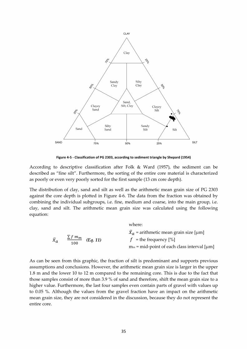
35

Figure 4-5 - Classification of PG 2303, according to sediment triangle by Shepard (1954)

According to descriptive classification after Folk & Ward (1957), the sediment can be described as “fine silt”. Furthermore, the sorting of the entire core material is characterized as poorly or even very poorly sorted for the first sample (13 cm core depth).

The distribution of clay, sand and silt as well as the arithmetic mean grain size of PG 2303 against the core depth is plotted in Figure 4-6. The data from the fraction was obtained by combining the individual subgroups, i.e. fine, medium and coarse, into the main group, i.e. clay, sand and silt. The arithmetic mean grain size was calculated using the following equation:

�̅�𝑎 = ∑𝑓 𝑚𝑠100

(Eq. 11)

where:

�̅�𝑎 = arithmetic mean grain size [µm] 𝑓 = the frequency [%] mm = mid-point of each class interval [µm]

As can be seen from this graphic, the fraction of silt is predominant and supports previous assumptions and conclusions. However, the arithmetic mean grain size is larger in the upper 1.8 m and the lower 10 to 12 m compared to the remaining core. This is due to the fact that those samples consist of more than 3.9 % of sand and therefore, shift the mean grain size to a higher value. Furthermore, the last four samples even contain parts of gravel with values up to 0.05 %. Although the values from the gravel fraction have an impact on the arithmetic mean grain size, they are not considered in the discussion, because they do not represent the entire core.

36

Figure 4-6 - Arithmetic mean grain size for PG 2303 as well as the distribution of Sand, Silt and Clay

37

Water content 4.4.

Overall, the water content in the sediment core decreases with increasing depth as illustrated in Figure 4-7. In the upper 2.5 m there is a strong variation detectable. It can be assumed that this is related to the composition of the core in this segment. Porous, unconsolidated material has high water content, however, under pressure from recent sediment layers pore volume decreases and therefore reduces the volume of water within the sediment (Füchtbauer, 1988).

Figure 4-7 - Water content of PG 2303

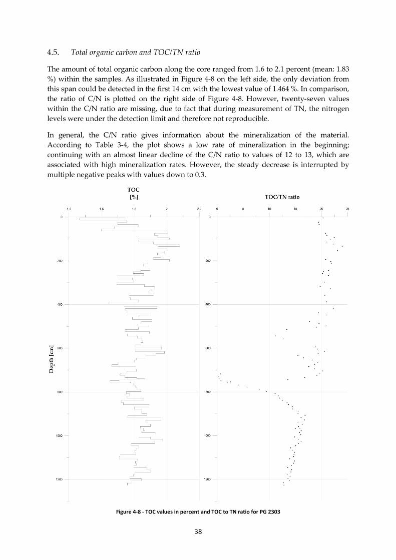
38

Total organic carbon and TOC/TN ratio 4.5.

The amount of total organic carbon along the core ranged from 1.6 to 2.1 percent (mean: 1.83 %) within the samples. As illustrated in Figure 4-8 on the left side, the only deviation from this span could be detected in the first 14 cm with the lowest value of 1.464 %. In comparison, the ratio of C/N is plotted on the right side of Figure 4-8. However, twenty-seven values within the C/N ratio are missing, due to fact that during measurement of TN, the nitrogen levels were under the detection limit and therefore not reproducible.

In general, the C/N ratio gives information about the mineralization of the material. According to Table 3-4, the plot shows a low rate of mineralization in the beginning; continuing with an almost linear decline of the C/N ratio to values of 12 to 13, which are associated with high mineralization rates. However, the steady decrease is interrupted by multiple negative peaks with values down to 0.3.

Figure 4-8 - TOC values in percent and TOC to TN ratio for PG 2303

39

In order to place the peaks into context, there are two possible approaches. The first assumption is based on clay content. A portion of clay minerals, for instance illite, are able to bind cations and positively charged ammonium ions, among others. This incorporation of inorganic nitrogen and the following analysis of those into the total amount of nitrogen, leads to negative changes in the TOC/TN ratio, while TOC remains almost the same. (Chesworth, 2008; Polubesova, 1999; Schroeder & Ingall, 1994)

Fortunately, a sample from the grain size analysis (593 cm) was placed in the surrounding of the first peak to assess this first approach. The results show a significant increase of the clay fraction up to 2 %, favoring the theory of incorporated nitrogen. However, since there is no available grain size sample at those lower C/N values, it could only be assumed that this approach applies to the first peak. At the second negative peak, a significant change of the clay fraction is not detectable.

The second assumption could be based on the theory of an external organic matter source. Looking at the data at the second peak from 700 to 800 cm, nitrogen values are strongly increasing (from 0.16 % to 6.4 %) compared to the arithmetic mean concentration without the peak of 0.13 % over the entire core. The TOC values are not changing very drastically within the same range.

In general, the mineralization of organic nitrogen and carbon from biological degradation is almost 1:1 (Thamdrup & Fleischer, 1998). However, due to oxygen depletion and therefore a deficiency in lower layers of a water column, the anaerobic ammonification is predominant and results in an increase of ammonium within the sediment (Kristensen & Blackburn, 1987; Vanderborght, Wollast, & Billen, 1977). As mentioned before, this ammonium gets incorporated into the clay fraction, and is thus traceable as inorganic nitrogen in the TN analysis. To summarize this assumption, it could be assumed that the second peak within the TOC/TN ratio diagram is related to a combination of external organic matter source, which cannot be further determined, and the composition of the grain size within this segment of the core.

δ13C 4.6.

The calculated values of δ13C against the core depth are plotted in Figure 4-9. The values primarily vary between -26.0 and -26.4 ‰ vs. VPDB, while lower values of approx. -26.5 ‰ vs. VPDB are reached only three times. However, those indicated spikes in the graph show no correlation with other values associated with the core.

From the ratio of δ13C itself, it can be assumed that the past biota primarily used the C3

pathway (or Calvin-Benson pathway). Furthermore, it is hypothesized that atmospheric CO2 was the prevailing source of carbon, suggesting that the found deposit could originate from terrestrial biota or used dissolved CO2, instead of bicarbonate.

In order to place those values in a broader context, the comparison of δ13C and C/N within a graph should establish this context. The following subchapter will frame this issue using the graphic from Meyers (1997).

40

Figure 4-9 - δ13

C values of PG 2303

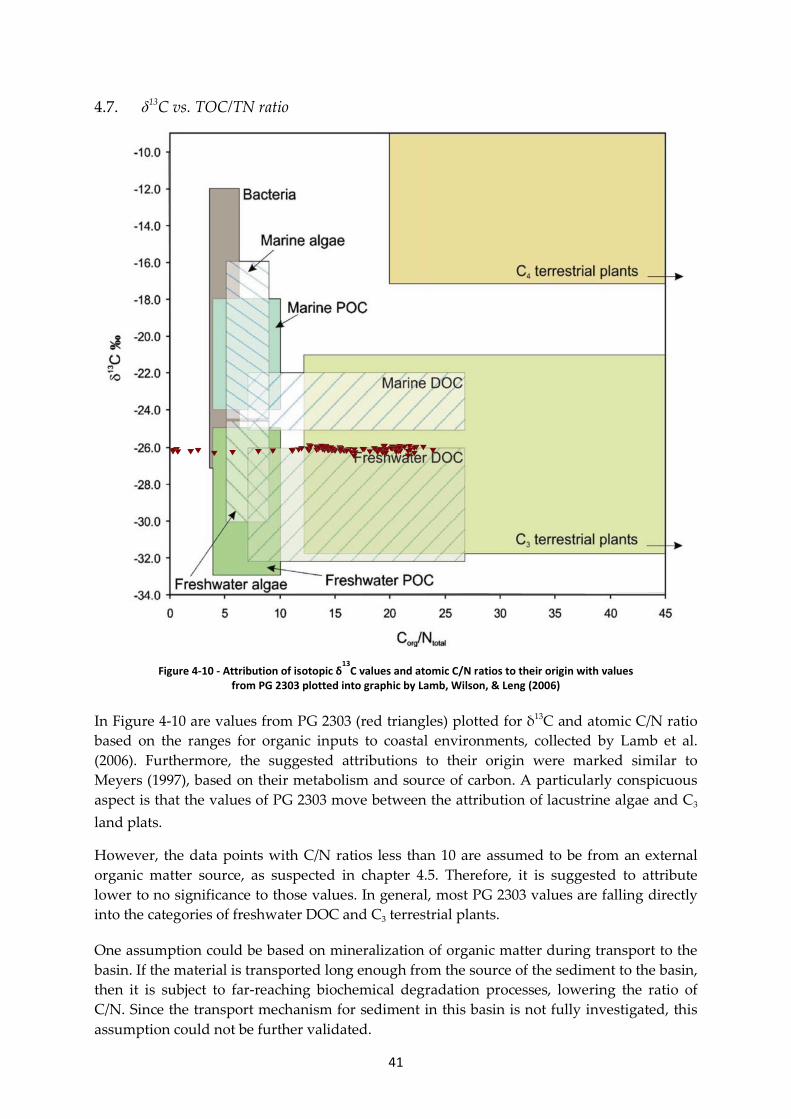
41

δ13C vs. TOC/TN ratio 4.7.

Figure 4-10 - Attribution of isotopic δ13

C values and atomic C/N ratios to their origin with values from PG 2303 plotted into graphic by Lamb, Wilson, & Leng (2006)

In Figure 4-10 are values from PG 2303 (red triangles) plotted for δ13C and atomic C/N ratio based on the ranges for organic inputs to coastal environments, collected by Lamb et al. (2006). Furthermore, the suggested attributions to their origin were marked similar to Meyers (1997), based on their metabolism and source of carbon. A particularly conspicuous aspect is that the values of PG 2303 move between the attribution of lacustrine algae and C3 land plats.

However, the data points with C/N ratios less than 10 are assumed to be from an external organic matter source, as suspected in chapter 4.5. Therefore, it is suggested to attribute lower to no significance to those values. In general, most PG 2303 values are falling directly into the categories of freshwater DOC and C3 terrestrial plants.

One assumption could be based on mineralization of organic matter during transport to the basin. If the material is transported long enough from the source of the sediment to the basin, then it is subject to far-reaching biochemical degradation processes, lowering the ratio of C/N. Since the transport mechanism for sediment in this basin is not fully investigated, this assumption could not be further validated.

42

14C dating 4.8.

Figure 4-11- Age-depth model of PG 2303

In order to determine the age of the core, the obtained raw data from the 14C dating had to be calibrated and processed. For this step, the R age-depth modelling package “Bacon” was used that “uses Bayesian statistics to reconstruct Bayesian accumulation histories for deposits” (Blaauw & Christen, 2013) (see also Appendix A6). The implemented data were then calibrated using one of the multiple preinstalled calibration curves as well as an initial offset.

For this thesis the calibration curve “Marine13” (Blaauw & Christen, 2013; Reimer et al., 2013) was selected, due to the position of the core in a coastal area. Calibration curves are needed, because the exchange of atmospheric 14CO2 with the hydrosphere can vary with the

production of 14CO2 in time and space (Reimer et al., 2013) and marine organisms are

exposed to different levels of 14C, which is known as the “reservoir effect”(Cao, Fairbanks, Mortlock, & Risk, 2007; Stuiver & Braziunas, 1993). Furthermore, Reimer et al. (2013) suggest to apply an additional offset, due to the fact that the curves are based on tropical and subtropical records and therefore can change in higher latitudes.

The Marine13 calibration curve has an implemented reservoir offset of 405 14C years (Reimer et al., 2013). However, after multiple test runs and due to the recommendation by Reimer et al. (2013), an additional offset of 700 years (with an associated error of ± 100 years) was applied, which resulted in a final total reservoir effect of 1,100 years. The calcareous material was then calibrated as displayed in Table 4-1 with their deviation.

43

Table 4-1 - Radiocarbon dates from AMS and age-depth modelling

Sample ID Cumulative Depth [cm]

Uncalibrated 14C [a BP]

Calibrated age ranges 2σ [cal a BP]

Weighted mean age [cal a BP]

Dated material

C[µg]

COL4367.1.1 151 1865 ± 41 357 - 686 532 Nuculana sp. 1000

COL4368.1.1 673.5 3062 ± 47 2044 - 2444 2239 Nuculana sp. 651

COL4369.1.1 816 3605 ± 54 2571 - 2950 2755 Nuculana sp. 686

COL4370.1.1 1043.5 4430 ± 52 3443 - 3800 3626 Nuculana sp. 651

COL4371.1.1 1135.5 4793 ± 89 3786 - 4134 3966 Nuculana sp. 209

COL4372.1.1 1174 4816 ± 51 3919 - 4265 4099 Nuculana sp. 686

COL4373.1.1 1214 4983 ± 50 4044 - 4403 4231 Nuculana sp. 651

COL4374.1.1 1228 4924 ± 48 4073 - 4439 4259 Nuculana sp. 884

At the same time, “Bacon” calculated the ages for the corresponding depths within the core. For this purpose, the core was sliced into 244 individual five centimeter sections and after 54 million Markov Chain Monte Carlo iterations, the model proposed a confident plot as displayed in Figure 4-11. Under these conditions, confident means that 95% of the iterations showed a similar pattern.

Additional information could be collected from the accumulation rate and the memory, which are both plotted in the upper section of Figure 4-11. Accumulation rate (“acc. mean”) is the reciprocal function of the average sedimentation rate, which, by implication, yields an average annual sedimentation rate of 0.33 cm/a. On the other hand, the memory (“mem.mean”) defines how much the sedimentation rate has changed over time. If this value is low, it means that the environmental conditions have changed significantly, while a higher memory assumes a constant, non-disruptive sedimentation. From the value 0.4 it can be concluded that the sedimentation was subject to change. (cf. Blaauw & Christen (2013))

44

This section of the work deals with the hypotheses that were given in the scope of this thesis. For this purpose, the data from the analysis and the literature were consulted. This chapter is therefore divided into three parts. The first part is linked to the origin of the sediment found in the core PG 2303. In the following subchapter, pathways of sediment and organic matter will be discussed. Finally, in the last part of the discussion, the aim is to understand the sedimentation process within the Herschel Basin.

Origin 5.1.

One of the main objectives of this thesis was to determine the source of the deposits found in the Herschel Basin sediment column. Previous studies have pointed out that the Mackenzie River is the predominant source of sediment and organic matter within the southern Beaufort Sea (Ayles & Snow, 2002; Carmack & Macdonald, 2002; Forbes, 1981; Giovando & Herlinveaux, 1981; Hill et al., 2001; Macdonald et al., 1998; Pelletier et al., 1984). However, the eventual percentage of those particles transported into the basin is still unclear, due to different influential factors that will be discussed in the following subchapter.

On the other hand, the various rivers and streams in the vicinity of the study area are contributing negligible amounts compared to the Mackenzie River (see Table 2-1). Therefore, coasts with progressive erosion within the immediate proximity will be considered as a third possible origin. Arctic permafrost coastlines are accounting for approx. 34% of the world’s coastlines, whereas the Canadian Beaufort Sea represents circa 5.6% of those arctic coastlines (M. Fritz et al., 2017; Günther et al., 2013; Lantuit, Overduin, et al., 2012). P. R. Hill et al. (1991) estimated that the total contribution of sediment from coastal erosion into the Canadian Beaufort Sea was ca. 5.62 x 106 t/a. The Yukon coast contributed 1.54 x 106 m³/a, which are 2.46 x 106 t/a, when assuming an average bulk density of 1.6 t/m³ (marine clays) (Hill et al., 1991). Still, this represents only a marginal share (~ 2%) compared to the mean annual suspended sediment discharge of the Mackenzie River (127 x 106 t/a).

Table 5-1 - Estimated suspended sediment discharge of possible sources (Hill et al., 1991)

Source Estimated suspended sediment discharge [*106 t/a] Mackenzie River 127

Yukon Coast erosion 2.46

Other Yukon rivers 1.45

Nevertheless, Couture (2010) calculated that the Yukon Coastal Plain has an annual flux of soil organic carbon into the Beaufort Sea of 0.04 x 106 t/a. According to recent studies, the pool of carbon stored frozen in the permafrost landmasses and coasts is considered to be between 1.4 and 1.85 x 1012 t (Couture, 2010; Schuur et al., 2008; Tamocai et al., 2009). As mentioned in chapter 2.1.1, about 50 percent of the area of Canada is underlain by permafrost (French, 2007; Heginbottom et al., 2012), which includes 0.196 x 1012 t of soil organic carbon (Couture, 2010; Tarnokai, Ping, & Kimble, 2006).

5. Discussion

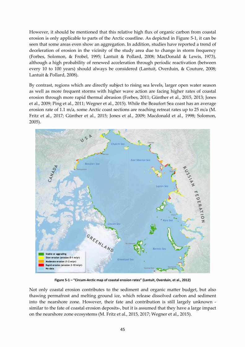
45

However, it should be mentioned that this relative high flux of organic carbon from coastal erosion is only applicable to parts of the Arctic coastline. As depicted in Figure 5-1, it can be seen that some areas even show an aggregation. In addition, studies have reported a trend of deceleration of erosion in the vicinity of the study area due to change in storm frequency (Forbes, Solomon, & Frobel, 1995; Lantuit & Pollard, 2008; MacDonald & Lewis, 1973), although a high probability of renewed acceleration through periodic reactivation (between every 10 to 100 years) should always be considered (Lantuit, Overduin, & Couture, 2008; Lantuit & Pollard, 2008).

By contrast, regions which are directly subject to rising sea levels, larger open water season as well as more frequent storms with higher wave action are facing higher rates of coastal erosion through more rapid thermal abrasion (Forbes, 2011; Günther et al., 2015, 2013; Jones et al., 2009; Ping et al., 2011; Wegner et al., 2015). While the Beaufort Sea coast has an average erosion rate of 1.1 m/a, some Arctic coast sections are reaching retreat rates up to 25 m/a (M. Fritz et al., 2017; Günther et al., 2015; Jones et al., 2009; Macdonald et al., 1998; Solomon, 2005).

Figure 5-1 – “Circum-Arctic map of coastal erosion rates” (Lantuit, Overduin, et al., 2012)

Not only coastal erosion contributes to the sediment and organic matter budget, but also thawing permafrost and melting ground ice, which release dissolved carbon and sediment into the nearshore zone. However, their fate and contribution is still largely unknown - similar to the fate of coastal erosion deposits-, but it is assumed that they have a large impact on the nearshore zone ecosystems (M. Fritz et al., 2015, 2017; Wegner et al., 2015).

46

Undoubtedly, in comparison with the Mackenzie River input, the contribution of organic matter seems quite small from the other possible sources (see Table 5-2). On the other hand, Fritz et al. (2015) pointed out that ice wedges within permafrost soils represent a significant DOC pool and should not be disregarded, especially regarding the increasing temperature during the ongoing climate change.

Table 5-2 - Estimated POC and DOC flux of possible sources after Couture (2010); Lantuit (2010) and Macdonald et al. (1998)

Source Estimated POC flux [*106 t/a] Estimated DOC flux [*106 t/a] Mackenzie River 2.1 1.3

Yukon Coast erosion 0.04 0.001

Other Yukon rivers 0.02 n/a

After the organic carbon from either riverine or terrestrial/coastal sources enters the Arctic Ocean, it is either exposed to bacterial degradation, exported offshore, or directly buried in the sediment column (Wegner et al., 2015). The information about the degradation and therefore a better understanding of the deposit is given by the C/N ratio as stated in chapter 4.5. It should be mentioned that the TOC, which was used in the C/N ratio, is the sum of POC, DOC and VOC (volatile organic carbon).

By contrast, information about the availability of nitrogen as a nutrient for organisms could not be collected from the amount of TN within the samples. The rates of ammonification and nitrification in the soil, which usually affect the total nitrogen content, are controlled by moisture and temperature (Baumann, He, Schmidt, Kühn, & Scholten, 2009; Maltby, 2009). Therefore, nitrogen is generally limited in tundra ecosystems and can even be lowered during coastal erosion, when ammonium is exposed to aerobic condition and hence, support nitrification and mineralization (Frey, McClelland, Holmes, & Smith, 2007; Harms, Abbott, & Jones, 2013). However, microbial activity is still highly connected to nitrogen availability and therefore represented within the C/N ratio.

Table 5-3 - Statistical calculation of C/N ratio and δ13

C values

Minimum Mean Maximum

C/N ratio 0.317(+) 15.820 23.960

δ13C [‰ vs. VPDB] -26.54 -26.18 -25.97 (+) This value was discussed in chapter 4.5 to be subject to an external organic carbon source.

The statistical evaluation for the two parameters C/N ratio and δ13C is given in Table 5-3. As indicated, the minimum value for C/N ratio was assumed to be subject to an external organic carbon source. By eliminating the peak from the data set, the mean value shifts to a ratio of approx. 17, whereas the minimum value would be set to around 13. This would suggest a moderate mineralization rate throughout the core (see Table 3-4).

In order to assign a possible source to the values from the core, it is necessary to extract data from the literature for fluvial, terrestrial and marine deposits in the near vicinity. According to Körner, Farquhar, & Wong (1991), this site specific literature search is inevitable, because there is an additional difference in δ13C values between latitudes (equatorial to Arctic zone) and even between hemispheres.

47

Figure 4-10 provides an initial classification by using the graphic by Lamb et al. (2006), which is based on compilation of data from multiple references for typical δ13C values and C/N ranges for organic inputs to coastal environments. Thus, the organic matter found in the sediment column of the Herschel Basin could be initially assigned to freshwater DOC.

However, paleoenvironmental reconstruction within marine bulk sediment might be affected by the presence of bacteria and algae as well as allochthonous material (Chmura, Aharon, Socki, & Abernethy, 1987; Lamb et al., 2006). An overview of δ13C values and C/N ranges compared to the obtained data from core PG 2303 is given in Table 5-4. On the first quantitative examination of Table 5-4, it can be seen that marine algae and phytoplankton are not the main source of the Herschel Basin deposit.

Table 5-4 - Typical δ13

C values and C/N ranges for organic inputs to coastal environments

δ13C [‰ vs. VPDB] range

C/N ratio References

Terrestrial plants(+) -32 ‰ to -21 ‰

} > 12

(Deines, 1980; Lamb et al., 2006; Meyers, 1997; Prahl, Bennett, & Carpenter, 1980; Tyson, 1995)

Freshwater plants -50 ‰ to -11 ‰ (Keeley & Sandquist, 1992; Lamb et

al., 2006; Osmond, Valaane, Haslam, Uotila, & Roksandic, 1981;

Prahl et al., 1980; Tyson, 1995)

Freshwater algae -30 ‰ to -26 ‰

}

< 10

(Lamb et al., 2006; Meyers, 1994; Schidlowski, Hayes, & Kaplan,

1983; Tyson, 1995)

Marine algae -23 ‰ to -16 ‰ (Haines, 1976; Lamb et al., 2006;

Meyers, 1994; Schubert & Calvert, 2001; Tyson, 1995)

Bacteria -27 ‰ to -12 % 4 - 6 (Coffin, Fry, Peterson, & Wright, 1989; Lamb et al., 2006; Meyers,

1994; Tyson, 1995)

Freshwater phytoplankton

POC: -30 ‰ to -25 ‰ DOC: -28 ‰ to -26 ‰

5 – 7

(Lamb et al., 2006; Meyers, 1994; Middelburg & Nieuwenhuize,

1998; Peterson, Fry, Hullar, Saupe, & Wright, 1994; Salomons & Mook,

1981; Tyson, 1995)

Marine phytoplankton

POC: -21 ‰ to -18 ‰ DOC: -25 ‰ to -22 ‰

< 8

(Bordovskiy, 1965; Lamb et al., 2006; Middelburg &

Nieuwenhuize, 1998; Peters, Sweeney, & Kaplan, 1978; Peterson et al., 1994; Yamaguchi, Montani,

Tsutsumi, Hamada, & Ueda, 2003)

Mackenzie River (POC) -34 % to -22‰ 9 – 23(++)

(K. A. Brown et al., 2014; Emmerton, Lesack, & Vincent,

2008; Macdonald, Naidu, Yunker, & Gobeil, 2004; Naidu et al., 2000)

Herschel Basin -26.18 ‰ 15.82 Mean values from this thesis

(+) This example only refers to C3-plants, due to the fact that there are the most abundant plants in this latitude (Ehleringer, 1979). (++) The ratio changes from upper reaches with higher values to the delta with relative lower values

48

Although Rau, Takahashi, & Marais (1989) pointed out that marine algae, which are present in cold polar sea waters, might have low δ13C values as their lacustrine counterpart (down to -28 ‰), but, due to their relatively lower C/N ratio between four and ten compared to the Herschel Basin value (Meyers, 1997), they are not primarily represented within the sediment column.

Therefore, it becomes obvious and more likely that the majority of organic carbon within the sediment derives from terrestrial sources. Nonetheless, to distinguish between different sources within mixed sediment from coastal areas can be difficult (Lamb et al., 2006). For instance, if terrestrial material is predominant, the mean value of δ13C could be increased through high marine algal production, while at the same time the C/N ratio decreases and thus, changing the significance of the obtained data (Chivas et al., 2001; Chmura & Aharon, 1995).

By looking at the C/N ratio from Herschel Basin - which by comparison is larger than most of the stated values - it can be seen that the value emphasizes three possible main sources: Mackenzie River, freshwater plants, and terrestrial plants.

However, due to degradation processes, the organic carbon content in the Mackenzie River decreases from the upper reaches to the delta. Hence, if implying an additional long-distance transport of organic matter from the Mackenzie delta to the Herschel Basin with a further biological degradation, then it can be hypothesized that the POC from Mackenzie River is not the main source of the Herschel Basin. Nevertheless, due to its large contribution of sediment and DOC into the Beaufort Sea, the Mackenzie River will be further assumed as possible input. But as mentioned previously in this chapter, the fate and contribution of dissolved organic carbon into the Arctic coastal waters is still unclear and therefore leaves no room for interpretation (Dunton et al., 2006; M. Fritz et al., 2017).

This would suggest that the majority of organic matter from the Herschel Basin derives from nearby rivers, by transporting organic material from terrestrial material along the watercourse or just detached freshwater plants, or directly from terrestrial material through coastal erosion. Based on these findings, it is still impossible to generate the exact organic matter composition, due to the lack of information about the versatile inputs. However, the distinct contribution from terrestrial plants is still preserved in the marine C/N ratio, similar to the example that was given by Meyers (1997) and Ertel & Hedges (1985) where vascular plant debris (C/N: 30-40) was preserved in the coastal bulk marine sediment (C/N: 15), which supports the hypothesis of dominating terrestrial origin.

Distribution 5.2.

Given the fact that particles and organic matter derive primarily from terrestrial sources, the distribution from each source is affected by different transport mechanisms. As can be seen from Chapter 2.2.2 and 2.2.3, currents and ice processes can be attributed to the distribution of terrestrial material (Darby et al., 2009; Forest et al., 2016; Macdonald, Kuzyk, & Johannessen, 2015; Nürnberg et al., 1994; Reimnitz, Kempema, & Barnes, 1987). Those mechanisms, however, depend on different factors, which will be discussed next.

49

Sea-ice and ice floes are responsible for the transport of eroded material from the coasts to the shores and shelves as well as the resuspension of material in the ice gouging zone (see “sea-ice processes” in Chapter 2.2.3). The main influencing factors for this mechanism are solar radiation, wind, and air temperature. They control the summer-ice extent, the direction of the drift and the thickness of the persistent sea-ice / landfast ice (occurring seven to nine months each year), which could lead to changes in the transport process (Atkinson, 2005; Couture, 2010, after McGillvray, Agnew, McKay, Pilkington, & Hill, 1993).

Moreover, by reference to Chapter 2.2.3, the extended open water season will have an impact on the protection from high wave activity through less landfast ice at the coasts. Thus, more terrestrial material would be transported into the nearshore zone and in return, produce more greenhouse gases. This initiates a temperature–feedback; it will raise temperature and therefore accelerate the reduction of sea-ice even more in the following years.

However, the advance of sea-ice has a seasonal dependency, whereas the transport of sediment through currents acts perennially. The strength and direction of the current although are affected by a variation of different factors (Darby et al., 2009; Forest et al., 2016; Pelletier & Medioli, 2014). A good summary of the perennial transport of riverine sediment into the ocean was given by Macdonald et al. (2015), which applies mainly for the Mackenzie river and therefore can be found as additional information in the Appendix A7 with explanations.

Since currents are part of a dynamic system, the factors that influence currents within the study area are salinity and temperature differences of inflowing water and the ocean, Coriolis force, ice-cover, and wind / atmospheric pressure (Carmack & Macdonald, 2002; Giovando & Herlinveaux, 1981; Macdonald et al., 2015; Pelletier et al., 1984; Pelletier & Medioli, 2014; Stopa et al., 2016). This is accompanied by the separation of grain size fractions into layers, while it also favors up- and downwelling processes, resuspension, and the formation of eddies.

As mentioned in Chapter 2.2.2, mostly longshore currents occur in the study area, whereas tidal currents are generally weak in the region (Carmack & Macdonald, 2002; Forbes, 1981). However, the fluvial input from Mackenzie River is affected by surface and longshore currents. For instance, the dominant wind direction in the study area is north-west (~310°) that leads to a south-eastward longshore and surface current, which also favors a downwelling of the Mackenzie River input (Burn, 2012; Carmack, Macdonald, & Jasper, 2004; Hill, 1990; Manson & Solomon, 2007). During May and August, the wind additionally tends to blow from the south-east (~120°), which drives the surface plume with additional cold, brackish water offshore near the Herschel Basin, caused by an upwelling at the shore with resuspension of sediment from lower water layers (Bouchard, 1974; Burn, 2012; Carmack & Macdonald, 2002; Hill et al., 1991).

When the sea-ice extent almost reaches the coast, the currents usually get weaker, due to the shielding by the ice sheet from the wind. Although the discharge of rivers in the area is lower during the winter period, they still can produce a freshwater lens or even a freshwater lake underneath the landfast ice sheet, due to differences in salinity. The Mackenzie River, for instance, forms a lake (“Lake Herlinveaux”) with a volume of 70 km³ and a spatial extent of 12,000 km², which would rank among the top 20 lakes worldwide by area. (cf. Carmack & Macdonald (2002), Carmack et al. (2004) and Dunton et al. (2006))

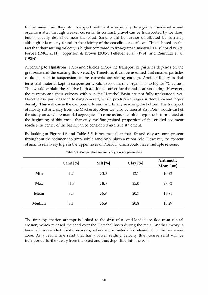
50

In the meantime, they still transport sediment – especially fine-grained material – and organic matter through weaker currents. In contrast, gravel can be transported by ice floes, but is usually deposited near the coast. Sand could be further distributed by currents, although it is mostly found in the vicinity of the coastline or outflows. This is based on the fact that their settling velocity is higher compared to fine-grained material, i.e. silt or clay. (cf. Forbes (1981, 2011), Jorgenson & Brown (2005), Pelletier et al. (1984) and Reimnitz et al. (1985))

According to Hjulström (1935) and Shields (1936) the transport of particles depends on the grain-size and the existing flow velocity. Therefore, it can be assumed that smaller particles could be kept in suspension, if the currents are strong enough. Another theory is that terrestrial material kept in suspension would expose marine organisms to higher 14C values. This would explain the relative high additional offset for the radiocarbon dating. However, the currents and their velocity within in the Herschel Basin are not fully understood, yet. Nonetheless, particles tend to conglomerate, which produces a bigger surface area and larger density. This will cause the compound to sink and finally reaching the bottom. The transport of mostly silt and clay from the Mackenzie River can also be seen at Kay Point, south-east of the study area, where material aggregates. In conclusion, the initial hypothesis formulated at the beginning of this thesis that only the fine-grained proportion of the eroded sediment reaches the center of the basin, can be considered as a true statement.

By looking at Figure 4-6 and Table 5-5, it becomes clear that silt and clay are omnipresent throughout the sediment column, while sand only plays a minor role. However, the content of sand is relatively high in the upper layer of PG2303, which could have multiple reasons.

Table 5-5 - Comparative summary of grain size parameters

Sand [%] Silt [%] Clay [%] Arithmetic Mean [µm]

Min 1.7 73.0 12.7 10.22

Max 11.7 78.3 25.0 27.82

Mean 3.5 75.8 20.7 16.81

Median 3.1 75.9 20.8 15.29

The first explanation attempt is linked to the drift of a sand-loaded ice floe from coastal erosion, which released the sand over the Herschel Basin during the melt. Another theory is based on accelerated coastal erosions, where more material is released into the nearshore zone. As a result, fine sand that has a lower settling velocity than coarse sand will be transported further away from the coast and thus deposited into the basin.

51

Sedimentation 5.3.

In order to describe the sedimentation volume, values from C/N ratio and age-depth model will be considered. Although a distinctive transition between possible layers / facies was not detectable visually, the almost consistent decline of the C/N ratio with increasing depth (see Figure 4-8) supports the theory of a constant accumulation of sediment within the basin and an increasing degradation process.

If considering the average annual sedimentation rate by the age-depth model of 0.33 cm/a, the average annual sediment and carbon deposition into the basin is calculated as follows:

AHerschelBasin * vsedimentation = QHerschelBasin (Eq. 12)

=> 127,000,000 m² * 0.0033 m/a = 423,333 m³/a

QHerschelBasin * ρ = m (Eq. 13)

=> 423,333 m³ * 1,700 kg/m³ = 719,666 t/a

where: QHerschelBasin = sediment flux [m³/a]

AHerschelBasin = estimated area [m²] (see Chapter 2)

vsedimentation = sedimentation rate [cm/a]

ρ = average density of PG 2303 [kg/m³] m = annual deposit [t/a]

On average, approx. 720,000 tons of sediment will be deposit annually into the Herschel Basin. On the other hand, when expecting an average TOC content of 1.83 % (see Chapter 4.5), ca. 13,200 tons of organic carbon will be accumulated every year in the marine sediment. However, if assuming that the coastal erosion hasn’t changed significantly since 1991 and that the Yukon rivers (except Mackenzie) and coastal erosion are the main contributors to the Herschel Basin, then approx. a fifth of the erosion surveyed by Hill et al. (1991) (Table 5-1) would have been deposited within the Herschel Basin.

Of course, this will raise the questions of the location and quantity of remaining material from the inputs, especially, if considering the additional input from Mackenzie River, an increase in air temperature and consequently, an increase in erosion rates. Those questions are somehow related to the transport mechanisms, mentioned in the previous subchapter. Nevertheless, those questions will remain unanswered within the thesis, due to multiple unknown variables.

Firstly, coastal erosion is the landward retreat of coastlines and although volumetrically observed, the individual grain-size data for every erosion event is nearly impossible to obtain or predict. For instance, the Yukon coastal plain is covered by Pleistocene and Holocene unconsolidated deposits, similar to Herschel Island, which is covered by glacial deposits, while it is mainly composed (poorly sorted) of silty clay with pebbles, silt, sand, and marine Pleistocene fossils (M. Fritz et al., 2012; Rampton, 1982). According to Rampton (1982) the majority of coarse material is deposited near beaches and spits. This would lower the estimated volume of material that could possibly be kept in suspension.

Secondly, the hydraulic conditions within the basin are still largely unexplored. Since the settling in the basin is depending on the flow velocity of the currents, the particle distribution and sedimentation can only be estimated. On the other hand, not all particles can be kept in suspension and therefore will settle with a high probability in the nearshore zone (M. Fritz et al., 2017; Günther et al., 2013)

52

The aim of this Master’s thesis was to quantify the amount of carbon, nitrogen and sediment with terrestrial origin throughout the sediment column from the Herschel Basin. The increasing research effort to understand the dynamics of Arctic coasts is justified by their contribution to the global carbon budget and their vulnerability. As shown in Chapter 2, the study area of this Master’s thesis was set within a unique surrounding, which is already subject to processes that will change the coastline drastically due to climate change. The core from the Herschel Basin was then analyzed in order to obtain data of biogeochemical and sedimentary parameters, according to the methods mentioned in Chapter 3. Subsequently, the represented values were discussed in the context of the study area and available literature.

The results showed that the majority of sediment found in the sediment column of the Herschel Basin could be assigned to a mix of riverine and terrestrial/coastal inputs. However, the individual percentage of each input (marine, fluvial and terrestrial) could not be distinguished, due to lack of data. Additionally, the influence of the Mackenzie River was only partially answered.

Kuzyk, Macdonald, & Johannessen (2015) suggested using simple mixing models, which would account for the complexity of mixing rate, mixing depth and sedimentation rate within the basin. On contrast, for a mixing model the inflows should be known to some extent. Until now, there are no estimations or comprehensive summaries about the overall material (particles/DOC) that is currently floating in the ocean that could have an influence on the system.

Furthermore, the Herschel Basin addresses only a small portion of the overall erosion within the study area. Therefore it can be assumed with a high probability that the remaining organic matter and particles are deposited within the nearshore zone, although resuspension will change the net accumulation. If the suspected constant sedimentation rate found in the Herschel Basin also applies to the remaining area, the area between Thetis Bay and Philips Bay are likely to be filled each year by 0.33 cm/a with organic-rich sediment. This will have an negative impact on “[…] climate feedbacks, on nearshore food webs, and on local communities, whose survival still relies on marine biological resources”(M. Fritz et al., 2017). Additionally, this would support the third hypothesis (“High accumulation rates on the shelf remove substantial amounts of carbon from the Arctic carbon cycle”). However, the mechanisms that are driving the transportation of particles within the basin are not fully understood, in which case this hypothesis could not be completely validated.

In contrast, as anticipated in the beginning of this Master’s thesis, most of the hypotheses can be confirmed. If assuming that only adjacent rivers and coastal erosion are the main contributor to the sedimentation, then “only a part [up to a fifth of the available material] of the organic carbon and nitrogen stored in the coastal permafrost is accumulated in the marine sediment record of Herschel Basin” (hypothesis no. 1). A higher rate of coastal erosion will also increase the sedimentation within the basin, but also in the rest of the nearshore zone. Further research of the nearshore zone is therefore recommended.

6. Conclusion

53

The material found in the sediment column has a strong terrestrial background (high δ13C values), but is already moderately degraded, which suggests that “the biogeochemical quality of the eroded carbon changes from the source of the erosion to the accumulation in the basin”, in which case the second hypothesis could be confirmed.

Finally, the third hypothesis claimed that “only the fine-grained proportion of the eroded sediment reaches the center of the basin, whereas the large portion of eroded material will be transported through, for instance, currents, ice push or resuspension to different locations”. The composition of the core PG 2303 primarily showed a clayey silt mixture, dominated by fine-grained sediment, which supports this theory.

In conclusion, this thesis showed that coastal erosion affected by climate change will have an impact on the Arctic nearshore zone. The study area represents a key storage site for Arctic research. It is proposed that future research should focus on the transport mechanisms within the study area. The use of isotopic tracers (e.g. Th – U – Pb) could be a possible solution as suggested by Goldstein & Hemming (2003) whereby input sizes and currents could be classified. Additionally, a higher resolution of the sediment and organic matter content through increased sampling around the Herschel Basin can be helpful in understanding the distribution and resuspension processes.

54

Ahnert, F. (1999). Einführung in die Geomorphologie (2nd ed.). Stuttgart: Ulmer.

Are, F. E. (1988). Thermal abrasion of sea coasts. Polar Geography and Geology 12.

Are, F. E., Reimnitz, E., Grigoriev, M. N., Hubberten, H. W., & Rachold, V. (2008). The Influence of Cryogenic Processes on the Erosional Arctic Shoreface. Journal of Coastal Research, 241, 110–121. https://doi.org/10.2112/05-0573.1

Atkinson, D. E. (2005). Observed storminess patterns and trends in the circum-Arctic coastal regime. Geo-Marine Letters, 25(2–3), 98–109. https://doi.org/10.1007/s00367-004-0191-0

Ayles, G. B., & Snow, N. B. (2002). Canadian Beaufort Sea 2000: The environmental and social setting. Arctic, 55(SUPPL. 1), 4–17.

Baumann, F., He, J. S., Schmidt, K., Kühn, P., & Scholten, T. (2009). Pedogenesis, permafrost, and soil moisture as controlling factors for soil nitrogen and carbon contents across the Tibetan Plateau. Global Change Biology, 15, 3001–3017.

Björck, S., & Wohlfarth, B. (2001). 14C Chronostratigraphic Techniques in Paleolimnology. Tracking Environmental Change Using Lake Sediments, 1, 205–245. https://doi.org/10.1007/0-306-47669-X_10

Blaauw, M., & Christen, J. A. (2013). Bacon manual – v2.2. Tutorial, 1–11.

Bordovskiy, O. K. (1965). Sources of organic matter in marine basins. Marine Geology, 3, 5–31.

Bouchard, M. (1974). Géologie des dépôts meubles de l’île Herschel, territoire du Yukon. Université de Montréal.

Brothers, L. L., Herman, B. M., Hart, P. E., & Ruppel, C. D. (2016). Subsea ice-bearing permafrost on the U.S. Beaufort Margin: 1. Minimum seaward extent defined from multichannel seismic reflection data. Geochemistry, Geophysics, Geosystems, 17(11), 4354–4365. https://doi.org/10.1002/2016GC006584

Brown, K. A., Mclaughlin, F., Tortell, P. D., Varela, D. E., Yamamoto-Kawai, M., Hunt, B., & Francois, R. (2014). Determination of particulate organic carbon sources to the surfacemixed layer of the Canada Basin, Arctic Ocean. Journal of Geophysical Research: Oceans, 119, 1084–1102. https://doi.org/10.1002/2013JC009197.Received

Brown, R. J. E., & Kupsch, W. O. (1974). Permafrost terminology. Quaternary Research, 5(3), 468. https://doi.org/10.1016/0033-5894(75)90043-5

Burn, C. R. (2012). Herschel Island—Qikiqtaryuk: A Natural and Cultural History. University of Calgary Press, 236.

Burn, C. R., & Zhang, Y. (2009). Permafrost and climate change at Herschel Island (Qikiqtaruq), Yukon Territory, Canada. Journal of Geophysical Research: Earth Surface, 114(2), 1–16. https://doi.org/10.1029/2008JF001087

Butler, R. F. (1998). Paleomagnetism: Magnetic domains to geologic terranes. Electronic Edition, September 2004. https://doi.org/10.1006/icar.2001.6754

7. References

55

Cao, L., Fairbanks, R. G., Mortlock, R. A., & Risk, M. J. (2007). Radiocarbon reservoir age of high latitude North Atlantic surface water during the last deglacial. Quaternary Science Reviews, 26(5–6), 732–742. https://doi.org/10.1016/j.quascirev.2006.10.001

Carmack, E. C., & Macdonald, R. W. (2002). Oceanography of the Canadian shelf of the Beaufort Sea: A setting for marine life. Arctic, 55(SUPPL. 1), 29–45. https://doi.org/10.1126/science.100.2596.291

Carmack, E. C., Macdonald, R. W., & Jasper, S. (2004). Phytoplankton productivity on the Canadian Shelf of the Beaufort Sea. Marine Ecology Progress Series, 277, 37–50. https://doi.org/10.3354/meps277037

Chelys. (2010). Sediments Pour from Mackenzie River into Beaufort Sea, Canada. Chelys srl / EOSNAP. Retrieved from http://www.eosnap.com/public/media/2010/10/canada/20100907-canada-full.jpg

Chesworth, W. (2008). Encyclopedia of soil science (2nd ed.). Dordrecht: Springer.

Chivas, A. R., García, A., van der Kaars, S., Couapel, M. J. J., Holt, S., Reeves, J. M., … Cecil, C. B. (2001). Sea-level and environmental changes since the last interglacial in the Gulf of Carpentaria, Australia: An overview. Quaternary International, 82(85), 19–46. https://doi.org/10.1016/S1040-6182(01)00029-5

Chmura, G. L., & Aharon, P. (1995). Stable carbon isotope signatures of sedimentary carbon in coastal wetlands as indicators of salinity regime. Journal of Coastal Research, 11, 124–135.

Chmura, G. L., Aharon, P., Socki, R. A., & Abernethy, R. (1987). An inventory of 13C abundances in coastal wetlands of Louisiana, USA: vegetation and sediments. Oecologia, 74(2), 264–271. https://doi.org/10.1007/BF00379369

Clark, I. D., & Fritz, P. (1997). Environmental isotopes in hydrology. Boca Raton: Lewis Publishers.

Cockburn, J. M. H., & Lamoureux, S. F. (2008). Hydroclimate controls over seasonal sediment yield in two adjacent High Arctic watersheds. Hydrological Processes, 22(12), 2013–2027. https://doi.org/10.1002/hyp.6798

Coffin, R. B., Fry, B., Peterson, B. J., & Wright, R. T. (1989). Carbon isotopic compositions of estuarine bacteria. Limnology and Oceanography, 34, 1305 – 1310.

Couture, N. (2010). Fluxes of Soil Organic Carbon From Eroding Permafrost Coasts, Canadian Beaufort Sea. McGill University, Montreal.

Craig, H. (1953). The geochemistry of the stable carbon isotopes. Geochimica et Cosmochimica Acta, 3(2–3), 53–92. https://doi.org/10.1016/0016-7037(53)90001-5

Dansgaard, W. (1953). Comparative measurements of standards for carbon isotopes. Geochimica et Cosmochimica Acta, 3(5), 253–256. https://doi.org/10.1016/0016-7037(53)90044-1

Darby, D. A., Ortiz, J., Polyak, L., Lund, S., Jakobsson, M., & Woodgate, R. A. (2009). The role of currents and sea ice in both slowly deposited central Arctic and rapidly deposited Chukchi-Alaskan margin sediments. Global and Planetary Change, 68(1–2), 58–72. https://doi.org/10.1016/j.gloplacha.2009.02.007

Dearing, J. A. (1999). Environmental Magnetic Susceptibility Using the Bartington MS2 System, 52 pp.

Degens, E. T. (1969). Biogeochemistry of stable carbon isotopes. In G. Eglington & M. T. J. Murphy (Eds.), Organic Geochemistry (pp. 304–329). Springer Berlin.

56

Deines, P. (1980). The isotopic composition of reduced organic carbon. In P. Fritz & J. C. Fontes (Eds.), Handbook of Environmental Isotope Geochemistry (p. 329-406 ). Amsterdam: Elsevier.

Duk-Rodkin, A., Barendregt, R. W., Froese, D. G., Weber, F., Enkin, R., Rod Smith, I., … Klassen, R. (2004). Timing and extent of plio-pleistocene glaciations in north-western canada and east-central alaska. In Developments in Quaternary Science (Vol. 2, pp. 313–345). https://doi.org/10.1016/S1571-0866(04)80206-9

Dunton, K. H., Weingartner, T., & Carmack, E. C. (2006). The nearshore western Beaufort Sea ecosystem: Circulation and importance of terrestrial carbon in arctic coastal food webs. Progress in Oceanography, 71(2–4), 362–378. https://doi.org/10.1016/j.pocean.2006.09.011

Dyke, A. S., Andrews, J. T., Clark, P. U., England, J. H., Miller, G. H., Shaw, J., & Veillette, J. J. (2002). The Laurentide and Innuitian ice sheets during the Last Glacial Maximum. Quaternary Science Reviews, 21(1–3), 9–31. https://doi.org/10.1016/S0277-3791(01)00095-6

Dyke, A. S., & Prest, V. K. (1987). Late Wisconsinan and Holocene History of the Laurentide Ice Sheet. Géographie Physique et Quaternaire, 41(2), 237. https://doi.org/10.7202/032681ar

Ehleringer, J. R. (1979). Photosynthesis and photorespiration: biochemistry, physiology, and ecological implications. Hortscience, 14, 217–222.

Elementar Analysensysteme GmbH. (2002). Handbook Elementar Vario EL Ⅲ. Hanau.

Emmerton, C. A., Lesack, L. F. W., & Vincent, W. F. (2008). Mackenzie River nutrient delivery to the Arctic Ocean and effects of the Mackenzie Delta during open water conditions. Global Biogeochemical Cycles, 22(1), 1–15. https://doi.org/10.1029/2006GB002856

EN ISO 14688. (2016). 14688-1: Geotechnical investigation and testing‚ Identification and classification of soil‚ Part 1: Identification and description. British Standards Institution, 2nd, 22.

Engelkemeir, A. G., Hamill, W. H., Inghram, M. G., & Libby, W. F. (1949). The Half-Life of Radiocarbon (C14). Physical Review, 75(12), 1825–1833. https://doi.org/10.1103/PhysRev.75.1825

Environment and Climate Change Canada. (2016). Climate Trends and Variations Bulletin – Annual 2015. Retrieved from http://ec.gc.ca/sc-cs/default.asp?lang=En&n=7150CD6C-1

Ertel, J. R., & Hedges, J. I. (1985). Sources of sedimentary humic substances: vascular plant debris. Geochimica et Cosmochimica Acta, 49(10), 2097–2107. https://doi.org/10.1016/0016-7037(85)90067-5

Folk, R. L., & Ward, W. C. (1957). Brazos River bar; a study in the significance of grain size parameters. Journal of Sedimentary Research, 27(1), 3–26. https://doi.org/10.1306/74D70646-2B21-11D7-8648000102C1865D

Forbes, D. L. (1981). Babbage River delta and lagoon : hydrology and sedimentology of an Arctic estuarine system. University of British Columbia. https://doi.org/10.14288/1.0095397

Forbes, D. L. (2011). State of the Arctic Coast 2010. Arctic. Retrieved from http://ipa.arcticportal.org/files/sac/state of the arctic rept.pdf

Forbes, D. L., Solomon, S. M., & Frobel, D. (1995). Report of the 1992 coastal surveys in the Beaufort Sea.

Forbes, D. L., & Taylor, R. B. (1994). Ice in the shore zone and the geomorphology of cold coasts. Progress in Physical Geography (Vol. 18). https://doi.org/10.1177/030913339401800104

57

Forest, A., Osborne, P. D., Curtiss, G., & Lowings, M. G. (2016). Current surges and seabed erosion near the shelf break in the Canadian Beaufort Sea: A response to wind and ice motion stress. Journal of Marine Systems, 160, 1–16. https://doi.org/10.1016/j.jmarsys.2016.03.008

French, H. M. (2007). The Periglacial Environment (Thrid). West Sussex, England: John Wiley & Sons Ltd,. https://doi.org/10.1002/9781118684931

French, H. M., & Shur, Y. (2010). The principles of cryostratigraphy. Earth-Science Reviews. https://doi.org/10.1016/j.earscirev.2010.04.002

Frey, K. E., McClelland, J. W., Holmes, R. M., & Smith, L. C. (2007). Impacts of climate warming and permafrost thaw on the riverine transport of nitrogen and phosphorus to the Kara Sea. Journal of Geophysical Research, 112, 2156–2202. https://doi.org/10.1029/2006JG000369

Fritz, M., Opel, T., Tanski, G., Herzschuh, U., Meyer, H., Eulenburg, A., & Lantuit, H. (2015). Dissolved organic carbon (DOC) in Arctic ground ice. Cryosphere, 9(2), 737–752. https://doi.org/10.5194/tc-9-737-2015

Fritz, M., Vonk, J. E., & Lantuit, H. (2017). Collapsing Arctic coastlines. Nature Climate Change 7, 6–7. https://doi.org/dx.doi.org/10.1038/nclimate3188

Fritz, M., Wetterich, S., Meyer, H., Schirrmeister, L., Lantuit, H., & Pollard, W. H. (2011). Origin and Characteristics of Massive Ground Ice on Herschel Island (Western Canadian Arctic) as revealed by Stable Water Isotope and Hydrochemical Signatures. Permafrost and Periglac. Process., 22(January), 26–38. https://doi.org/10.1002/ppp.714

Fritz, M., Wetterich, S., Schirrmeister, L., Meyer, H., Lantuit, H., Preusser, F., & Pollard, W. H. (2012). Eastern Beringia and beyond: Late Wisconsinan and Holocene landscape dynamics along the Yukon Coastal Plain, Canada. Palaeogeography, Palaeoclimatology, Palaeoecology, 319–320, 28–45. https://doi.org/10.1016/j.palaeo.2011.12.015

Füchtbauer, H. (1988). Sediment und Sedimentgestein (4th ed.). Stuttgart: E. Schweizbart’sche Verlagsbuchhandlung.

Geological Survey of Canada. (1975). Report of Activities Paper 75-1B. Ottawa.

Giovando, L. F., & Herlinveaux, R. H. (1981). A Discussion of Factors Influencing Dispersion of Pollutants in the Beaufort Sea. Pacific Marine Science Report, 81–4, 214.

Goldstein, S. L., & Hemming, S. R. (2003). Long-lived Isotopic Tracers in Oceanography, Paleoceanography, and Ice-sheet Dynamics. In Treatise on Geochemistry (pp. 453–489). Elsevier. https://doi.org/10.1016/B0-08-043751-6/06179-X

Gowan, E. J., Tregoning, P., Purcell, A., Montillet, J. P., & McClusky, S. (2016). A model of the western Laurentide Ice Sheet, using observations of glacial isostatic adjustment. Quaternary Science Reviews, 139, 1–16. https://doi.org/10.1016/j.quascirev.2016.03.003

Gruber, S. (2012). Derivation and analysis of a high-resolution estimate of global permafrost zonation. Cryosphere, 6(1), 221–233. https://doi.org/10.5194/tc-6-221-2012

Günther, F., Overduin, P. P., Sandakov, A. V., Grosse, G., & Grigoriev, M. N. (2012). Thermo-erosion along the Yedoma Coast of the Buor Khaya Peninsula, Laptev Sea, East Siberia. Tenth International Conference on Permafrost, 2, 137–142.

Günther, F., Overduin, P. P., Sandakov, A. V., Grosse, G., & Grigoriev, M. N. (2013). Short- and long-term thermo-erosion of ice-rich permafrost coasts in the Laptev Sea region. Biogeosciences, 10(6), 4297–4318. https://doi.org/10.5194/bg-10-4297-2013

58

Günther, F., Overduin, P. P., Yakshina, I. A., Opel, T., Baranskaya, A. V., & Grigoriev, M. N. (2015). Observing Muostakh disappear: Permafrost thaw subsidence and erosion of a ground-ice-rich Island in response to arctic summer warming and sea ice reduction. Cryosphere, 9(1), 151–178. https://doi.org/10.5194/tc-9-151-2015

Haines, E. B. (1976). Stable carbon isotope ratios in biota, soils and tidal water of a Georgia salt marsh. Estuarine and Coastal Marine Science, 4, 609–616.

Harms, T., Abbott, B. W., & Jones, J. B. (2013). Thermo-erosion gullies increase nitrogen available for hydrologic export. Biogeochemistry, 117(2–3), 299–311.

Hayes, J. . (1993). Factors controlling 13C contents of sedimentary organic compounds: Principles and evidence. Marine Geology, 113(1–2), 111–125. https://doi.org/10.1016/0025-3227(93)90153-M

Heginbottom, J. A., Brown, J., Humlum, O., & Svensson, H. (2012). Permafrost and periglacial environments. State of the Earth’s Cryosphere at the Beginning of the 21st Century: Glaciers, Global Snow Cover, Floating Ice, and Permafrost and Periglacial Environments, (December), 425–496.

Héquette, A., & Barnes, P. W. (1990). Coastal retreat and shoreface profile variations in the Canadian Beaufort Sea. Marine Geology, 91(1–2), 113–132. https://doi.org/10.1016/0025-3227(90)90136-8

Héquette, A., Ruz, M.-H., & Hill, P. R. (1995). The effects of the Holocene Sea Level Rise on the Evolution of the Southeastern Coast of the Canadian Beaufort Sea. Journal of Coastal Research, 11(2), 494–507.

Hill, P. R. (1987). Effect of sea ice on Beaufort Sea coastal processes. Geological Survey of Canada, Open File 1688.

Hill, P. R. (1990). Coastal Geology of the King Poing Area, Yukon Territory, Canada. Marine Geology, 91, 93–111.

Hill, P. R., Barnes, P., Héquette, A., & Ruz, M.-H. (1994). Arctic coastal plain shorelines. Coastal Evolution: Late Quaternary Shoreline Morphodynamics. Retrieved from http://books.google.com/books?hl=en&lr=&id=Asshp_VWANkC&oi=fnd&pg=PA341&dq=Arctic+coastal+plain+shorelines&ots=0TZswpWesd&sig=hJsg_jhGAOCcAthZPx0AaLdDWYM

Hill, P. R., Blasco, S. M., Harper, J. R., & Fissel, D. B. (1991). Sedimentation on the Canadian Beaufort Shelf. Continental Shelf Research, 11(8–10), 821–842.

Hill, P. R., Héquette, A., & Ruz, M.-H. (1993). Holocene sea-level history of the Canadian Beaufort shelf. Canadian Journal of Earth Sciences, 30(1), 103–108. https://doi.org/10.1139/e93-009

Hill, P. R., Lewis, C. P., Desmarais, S., Kauppaymuthoo, V., & Rais, H. (2001). The Mackenzie Delta: sedimentary processes and facies of a high-latitude, fine-grained delta. Sedimentology, 48, 1047–1078.

Hill, P. R., Mudie, P. J., Moran, K., & Blasco, S. M. (1985). A sea-level curve for the Canadian Beaufort Shelf. Canadian Journal of Earth Sciences, 22(10), 1383–1393. https://doi.org/10.1139/e85-146

Hill, P. R., & Nadeau, O. C. (1989). Storm-dominated Sedimentation on the Inner Shelf of the Canadian Beaufort Sea. SEPM Journal of Sedimentary Research, Vol. 59(3), 455–468. https://doi.org/10.1306/212F8FC1-2B24-11D7-8648000102C1865D

Hjulström, F. (1935). Studies of the morphological activity of rivers as illustrated by the River Fyris. Uppsala Universitet.

59

Hoefs, J. (2009). Stable isotope geochemistry (6th ed.). Berlin; Heidelberg: Springer, 2009.

Hollings, P., Schell, T. M., Scott, D. B., Rochon, A., & Blasco, S. M. (2008). Late Quaternary paleoceanography and paleo-sea ice conditions in the Mackenzie Trough and Canyon, Beaufort SeaThis article is one of a series of papers published in this Special Issue on the theme Polar Climate Stability Network . Canadian Journal of Earth Sciences, 45(11), 1399–1415. https://doi.org/10.1139/E08-054

House, N., & Fields, D. (2000). Multi-Sensor Core Logger Manual. Geotek.

Hu, K., Issler, D. R., Chen, Z., & Brent, T. A. (2013). Permafrost investigation by well logs, and seismic velocity and repeated shallow temperature surveys, Beaufort-Mackenzie Basin. Geological Survey of Canada, Open File 6956, 33. https://doi.org/10.4095/293120

IPCC. (2007). Climate change 2007 : impacts, adaptation and vulnerability : Working Group II contribution to the Fourth Assessment Report of the IPCC Intergovernmental Panel on Climate Change. Working Group II Contribution to the Intergovernmental Panel on Climate Change Fourth Assessment Report, 1(July), 976. https://doi.org/10.2134/jeq2008.0015br

IPCC, Stocker, T. F., Qin, D., Plattner, G.-K., Tignor, M. M. B., Allen, S. K., … Midgley, P. M. (2013). Climate Change 2013 - The Physical Science Basis. Intergovernmental Panel on Climate Change. https://doi.org/10.1038/446727a

Jakobsson, M., Andreassen, K., Bjarnadóttir, L. R., Dove, D., Dowdeswell, J. A., England, J. H., … Stein, R. (2014). Arctic Ocean glacial history. Quaternary Science Reviews, 92, 40–67. https://doi.org/10.1016/j.quascirev.2013.07.033

Jakobsson, M., Macnab, R., Mayer, L., Anderson, R., Edwards, M. E., Hatzky, J., … Johnson, P. (2008). An improved bathymetric portrayal of the Arctic Ocean: Implications for ocean modeling and geological, geophysical and oceanographic analyses. Geophysical Research Letters, 35(7), n/a-n/a. https://doi.org/10.1029/2008GL033520

Jones, B. M., Arp, C. D., Jorgenson, T. M., Hinkel, K. M., Schmutz, J. A., & Flint, P. L. (2009). Increase in the rate and uniformity of coastline erosion in Arctic Alaska. Geophysical Research Letters, 36(3), 1–5. https://doi.org/10.1029/2008GL036205

Jorgenson, T. M., & Brown, J. (2005). Classification of the Alaskan Beaufort Sea Coast and estimation of carbon and sediment inputs from coastal erosion. Geo-Marine Letters, 25(2–3), 69–80. https://doi.org/10.1007/s00367-004-0188-8

Keeley, J. E., & Sandquist, D. R. (1992). Carbon: Freshwater plants. Plant, Cell and Environment, 15, 1021–1035.

Keigwin, L. D., Donnelly, J. P., Cook, M. S., Driscoll, N. W., & Brigham-Grette, J. (2006). Rapid sea-level rise and Holocene climate in the Chukchi Sea. Geology, 34(10), 861. https://doi.org/10.1130/G22712.1

Kobayashi, N., Vidrine, J. C., Nairn, R. B., & Solomon, S. M. (1999). Erosion of frozen cliffs due to storm surge on Beaufort Sea Coast. Journal of Roastal Research, 15(2), 332–344. https://doi.org/10.2307/4298946

Körner, C., Farquhar, G. D., & Wong, S. C. (1991). Carbon isotope discrimination by plants follows latitudinal and altitudinal trends. Oecologia, 88(1), 30–40. https://doi.org/10.1007/BF00328400

60

Kottek, M., Grieser, J., Beck, C., Rudolf, B., & Rubel, F. (2006). World map of the Köppen-Geiger climate classification updated. Meteorologische Zeitschrift, 15(3), 259–263. https://doi.org/10.1127/0941-2948/2006/0130

Koven, C. D., Schuur, E. A. G., Schädel, C., Bohn, T. J., Burke, E. J., Chen, G., … Turetsky, M. (2015). A simplified, data-constrained approach to estimate the permafrost carbon–climate feedback. Philosophical Transactions of the Royal Society A: Mathematical, Physical and Engineering Sciences, 373(2054), 20140423. https://doi.org/10.1098/rsta.2014.0423

Kristensen, E., & Blackburn, T. H. (1987). The fate of organic carbon and nitrogen in experimental marine sediment systems: Influence of bioturbation and anoxia. J. Mar. Res., 45, 241–257.

Kurfurst, P. J., & Dallimore, S. R. (1989). Geological and geotechnical conditions of the Beaufort Sea coastal zone, Arctic Canada. Coastal Lowlands, 68, 121–129.

Kuzyk, Z. A., Macdonald, R. W., & Johannessen, S. C. (2015). Contaminant profiles in marine and estuarine sediments. In J. M. Blais, M. P. Rosen, & J. P. Smol (Eds.), Environmental Contaminants: Using Natrual Achives to Track Sources and Long-Term Trends of Pollution. Springer.

Lamb, A. L., Wilson, G. P., & Leng, M. J. (2006). A review of coastal palaeoclimate and relative sea-level reconstructions using d13C and C/N ratios in organic material. Earth-Science Reviews, 75(1–4), 29–57. https://doi.org/10.1016/j.earscirev.2005.10.003

Lambeck, K., Rouby, H., Purcell, A., Sun, Y., & Sambridge, M. (2014). Sea level and global ice volumes from the Last Glacial Maximum to the Holocene. Proceedings of the National Academy of Sciences of the United States of America, 111(43), 15296–303. https://doi.org/10.1073/pnas.1411762111

Lambert, S. J. (1995). The Effect of Enhanced Greenhouse Warming on Winter Cyclone Frequencies and Strengths. Journal of Climate, 8, 1447–1452.

Lantuit, H. (2004). Mapping Permafrost and ground-ice related coastal erosion on Herschel Island, Southern Beaufort Sea, Yukon Territory Canada. McGill University, Montréal.

Lantuit, H. (2010). DOC fluxes from the Yukon Coastal Plain. Unpublished.

Lantuit, H., Overduin, P. P., & Couture, N. (2008). Sensitivity of Coastal Erosion to Ground Ice Contents : An Arctic-Wide Study Based on the ACD Classification of Arctic Coasts. Ninth International Conference on Permafrost, (1990), 1025–1029.

Lantuit, H., Overduin, P. P., Couture, N., Wetterich, S., Are, F. E., Atkinson, D. E., … Vasiliev, A. (2012). The Arctic Coastal Dynamics Database: A New Classification Scheme and Statistics on Arctic Permafrost Coastlines. Estuaries and Coasts, 35(2), 383–400. https://doi.org/10.1007/s12237-010-9362-6

Lantuit, H., Overduin, P. P., & Wetterich, S. (2013). Recent progress regarding permafrost coasts. Permafrost and Periglacial Processes, 24(2), 120–130. https://doi.org/10.1002/ppp.1777

Lantuit, H., & Pollard, W. H. (2008). Fifty years of coastal erosion and retrogressive thaw slump activity on Herschel Island, southern Beaufort Sea, Yukon Territory, Canada. Geomorphology, 95(1–2), 84–102. https://doi.org/10.1016/j.geomorph.2006.07.040

61

Lantuit, H., Pollard, W. H., Couture, N., Fritz, M., Schirrmeister, L., Meyer, H., & Hubberten, H. W. (2012). Modern and Late Holocene Retrogressive Thaw Slump Activity on the Yukon Coastal Plain and Herschel Island, Yukon Territory, Canada. Permafrost and Periglacial Processes, 23(1), 39–51. https://doi.org/10.1002/ppp.1731

Libby, W. F. (1955). Radiocarbon dating (2nd ed.). University of Chicago Press.

Libby, W. F. (1961). Radiocarbon Dating: The method is of increasing use to the archeologist, the geologist, the meteorologist, and the oceanographer. Science, 133(3453), 621–629. https://doi.org/10.1126/science.133.3453.621

MacDonald, B. C., & Lewis, C. P. (1973). Geomorphic and sedimentologic processes of rivers and coasts, Yukon coastal Plain. Environmental-Social Committee, Northern Pipelines, Report.

Macdonald, R. W., Kuzyk, Z. Z. A., & Johannessen, S. C. (2015). The vulnerability of Arctic shelf sediments to climate change. Environmental Reviews, 479(September), 1–19. https://doi.org/10.1139/er-2015-0040

Macdonald, R. W., Naidu, A. S., Yunker, M. B., & Gobeil, C. (2004). The Beaufort Sea: Distribution, sources, fluxes, and burial of organic carbon. In R. Stein & R. W. Macdonald (Eds.), The Organic Carbon Cycle in the Arctic Ocea (p. 177–193 ). Berlin: Springer.

Macdonald, R. W., Paten, D. W., & Carmack, E. C. (1995). The freshwater budget and under-ice spreading of Mackenzie River water in the Canadian Beaufort Sea based on salinity and 18O/16O measurements in water and ice. Journal of Geophysical Research, 100, 895–919.

Macdonald, R. W., Solomon, S. M., Cranston, R. E., Welch, H. E., Yunker, M. B., & Gobeil, C. (1998). A sediment and organic carbon budget for the Canadian beaufort shelf. Marine Geology, 144(4), 255–273. https://doi.org/10.1016/S0025-3227(97)00106-0

Mackay, R. (1959). Glacier ice-thrust features of the Yukon Coast. Geographical Bulletin, 13, 5–21.

Mackay, R. (1972). Offshore Permafrost and Ground Ice, Southern Beaufort Sea, Canada. Canadian Journal of Earth Sciences, 9, 1550–1561.

Maltby, E. (2009). Functional Assessment of Wetlands: Towards Evaluation of Ecosystem Services. Cambridge: Woodhead Publishing Limited.

Malvern Instruments Ltd. (2013). Brochure Mastersizer 3000. Worcestershire. Retrieved from http://www.malvern.com/de/Assets/MRK1872.pdf

Manson, G. K., & Solomon, S. M. (2007). Past and future forcing of Beaufort Sea coastal change. Atmosphere-Ocean, 45(2), 107–122. https://doi.org/10.3137/ao.450204

McGillvray, D. G., Agnew, T. A., McKay, G. A., Pilkington, G. R., & Hill, M. C. (1993). Report summary of impacts of climatic change on the Beaufort sea-ice regime: Implications for the Arctic petroleum industry. Prepared for Climate Change Digest: Atmospheric Environment Service.

Meyers, P. A. (1994). Preservation of elemental and isotopic source identification of sedimentary organic matter. Chemical Geology, 114(3–4), 289–302. https://doi.org/10.1016/0009-2541(94)90059-0

Meyers, P. A. (1997). Organic geochemical proxies of paleoceanographic, plaeolimnologic, and plaeoclimatic processes. Organic Geochemistry, 27(5), 213–250.

Meyers, P. A., & Arbor, A. (2001). Sediment Organic Matter. In Tracking Environmental Change Using Lake Sediments. Volume 2: Physical and Geochemical Methods (Vol. 2, pp. 239–269).

62

Meyers, P. A., & Lallier-Vergès, E. (1999). Lacustrine sedimentary organic matter of Late Quaternary paleoclimates. Journal of Paleolimnology, 21(2), 345–372. https://doi.org/10.1023/A:1008073732192

Middelburg, J. J., & Nieuwenhuize, J. (1998). Carbon and nitrogen stable isotopes in suspended matter and sediments from the Schelde Estuary. Marine Chemistry, 60, 217–225.

Mudrov, Y. V. (2007). Merzlotnye yavleniya v kriolitozone ravnin i gor (Permafrost phenomena in mountain and plain cryolithozone - General terms and definitions). Moscow: Scientific World.

Mustapha, S. Ben, Larouche, P., & Dubois, J.-M. M. (2016). Spatial and temporal variability of sea-surface temperature fronts in the Beaufort Sea from high-resolution satellite data. Continental Shelf Research, 124, 134–141. https://doi.org/10.1016/j.csr.2016.06.001

Naidu, A. S., Cooper, L. W., Finney, B. P., Macdonald, R. W., Alexander, C., & Semiletov, I. P. (2000). Organic carbon isotope ratio (δ13C) of Arctic Amerasian Continental shelf sediments. International Journal of Earth Sciences, 89(3), 522–532. https://doi.org/10.1007/s005310000121

Nakai, N. (1972). Carbon isotopic variation and the paleoclimate of sediments from Lake Biwa. Proceedings of the Japanese Academy, Vol. 48, 516–521.

Nelson, F. E., Anisimov, O. a, & Shiklomanov, N. I. (2001). Subsidence risk from thawing permafrost. Nature, 410(6831), 889–890. https://doi.org/10.1038/35073746

Nürnberg, D., Wollenburg, I., Dethleff, D., Eicken, H., Kassens, H., Letzig, T., … Thiede, J. (1994). Sediments in Arctic sea ice: Implications for entrainment, transport and release. Marine Geology, 119(3–4), 185–214. https://doi.org/10.1016/0025-3227(94)90181-3

O’Connor, M. J. (1984). Surficial Geology and Granular Resources southeast of Herschel Island.

O’Leary, M. H. (1981). Carbon isotope fractionation in plants. Phytochemistry, 20(4), 553–567. https://doi.org/10.1016/0031-9422(81)85134-5

Oertel, G. F. (1972). Patterns of sediment transport at nearshore zones influenced by wave and tidal currents : a study utilizing fluorescent tracers, (72), 28.

Ogorodov, S. (2003). The Role of Sea Ice in the Coastal Zone Dynamics of the Arctic Seas. Water Resources, 30(5), 509–518. https://doi.org/10.1023/A:1025725113288

Osmond, C. B., Valaane, N., Haslam, S. M., Uotila, P., & Roksandic, Z. (1981). Comparisons of d13C values in leaves of aquatic macrophytes from different habitats in Britain and Finland; some implications for photosynthetic processes in aquatic plants. Oecologia, 50, 117–124.

Park, R., & Epstein, S. (1960). Carbon isotope fractionation during photosynthesis. Geochimica et Cosmochimica Acta, 21(1–2), 110–126. https://doi.org/10.1016/S0016-7037(60)80006-3

Pelletier, B. R., Bornhold, B. D., Buckley, D. E., Costaschuk, S., Forbes, D. L., Lewis, C. F. M., … Wong, S. C. (1984). Marine Science Atlas Of The Beaufort Sea - Sediment. Canadian Government.

Pelletier, B. R., & Medioli, B. E. (2014). Environmental Atlas of the Beaufort Coastlands. Geological Survey of Canada, Open File 7619, 271 pp. https://doi.org/10.4095/294601

Peltier, W. R. (2002). On eustatic sea level history: Last Glacial Maximum to Holocene. Quaternary Science Reviews, 21(1–3), 377–396. https://doi.org/10.1016/S0277-3791(01)00084-1

63

Peters, K. E., Sweeney, R. E., & Kaplan, I. R. (1978). Correlation of carbon and nitrogen stable isotopes in sedimentary organic matter. Limnology and Oceanography, 23, 598–604.

Peterson, B. J., Fry, B., Hullar, M., Saupe, S., & Wright, R. T. (1994). The distribution and stable carbon isotope composition of dissolved organic carbon in estuaries. Estuaries, 17, 111–121.

Péwé, T. L. (1969). The periglacial environment. In T. L. Péwé (Ed.), The Periglacial Environment (pp. 1–9). Montreal: McGill-Queen’s University Press.

Ping, C. L., Michaelson, G. J., Guo, L., Jorgenson, T. M., Kanevskiy, M., Shur, Y., … Liang, J. (2011). Soil carbon and material fluxes across the eroding Alaska Beaufort Sea coastline. Journal of Geophysical Research: Biogeosciences, 116(2), 1–12. https://doi.org/10.1029/2010JG001588

Pollard, W. H. (1998). Arctic Permafrost and Ground Ice. In E. Weatherhead & C. M. Morseth (Eds.), Chapter 11: Climate Change, Ozone and ultraviolet Radiation. Arctic Monitoring and Assessment Program (AMAP) Assessment Report (pp. 717–773).

Polubesova, T. (1999). Modeling of Organic and Inorganic Cation Sorption by Illite. Clays and Clay Minerals, 47(3), 366–374. https://doi.org/10.1346/CCMN.1999.0470313

Prahl, F. G., Bennett, J. T., & Carpenter, R. (1980). The early diagenesis of aliphatic hydrocarbons and organic matter in sedimentary particulates from Dabob Bay, Washington. Geochimica et Cosmochimica Acta, 44, 1967–1976.

Rachold, V., Are, F. E., Atkinson, D. E., Cherkashov, G., & Solomon, S. M. (2005). Arctic Coastal Dynamics (ACD): An introduction. Geo-Marine Letters, 25(2–3), 63–68. https://doi.org/10.1007/s00367-004-0187-9

Rachold, V., Grigoriev, M. N., Are, F. E., Solomon, S. M., Reimnitz, E., Kassens, H., & Antonow, M. (2000). Coastal erosion vs riverline sediment discharge in the Arctic shelf seas. International Journal of Earth Sciences, 89(3), 450–459. https://doi.org/10.1007/s005310000113

Rampton, V. N. (1982). Quaternary Geology of the Yukon Coastal Plain. Geological Survey of Canada, Open File 1144.

Rau, G. H., Takahashi, T., & Des Marais, D. J. (1989). Latitudinal variations in plankton δ13C: implications for CO2 and productivity in past oceans. Nature, 341(6242), 516–518. https://doi.org/10.1038/341516a0

Reimer, P. J., Bard, E., Bayliss, A., Beck, J. W., Blackwell, P. G., Bronk Ramsey, C., … van der Plicht, J. (2013). IntCal13 and Marine13 Radiocarbon Age Calibration Curves 0–50,000 Years cal BP. Radiocarbon, 55(4), 1869–1887. https://doi.org/10.2458/azu_js_rc.55.16947

Reimnitz, E., Barnes, P., & Harper, J. R. (1990). A review of beach nourishment from ice transport of shoreface materials, Beaufort Sea, Alaska. Journal of Coastal Research, 6(2), 439–469.

Reimnitz, E., Graves, S. M., & Barnes, P. W. (1985). Beaufort Sea Coastal Erosion, Shoreline Evolution, and Sediment Flux. U.S. Geological Survey Report 85-380, 78.

Reimnitz, E., Kempema, E. W., & Barnes, P. W. (1987). Anchor ice, seabed freezing, and sediment dynamics in shallow Arctic Seas. Journal of Geophysical Research, 92(C13), 14671. https://doi.org/10.1029/JC092iC13p14671

Reimnitz, E., & Maurer, D. K. (1979). Effects of Storm Surges on the Beaufort Sea Coast, Northern Alaska. Arcitc, 32(4), 329–344. Retrieved from http://pubs.aina.ucalgary.ca/arctic/Arctic32-4-329.pdf

64

Reimnitz, E., & Wolf, S. C. (1998). Are North Slope Surface Alluvial Fans Pre-Holocene Relicts ? U.S. Geological Survey, (Professional Paper 1605).

Rethemeyer, J., Fülöp, R., Höfle, S., Wacker, L., Heinze, S., Hajdas, I., … Dewald, A. (2013). Status report on sample preparation facilities for CologneAMS center C analysis at the new. Nuclear Inst. and Methods in Physics Research, B, 294, 168–172. https://doi.org/10.1016/j.nimb.2012.02.012

Romanovsky, V. E., Gruber, S., Instanes, A., Jin, H., Marchenko, S. S., Smith, S. L., … Walter, K. M. (2007). Frozen Ground (Chapter 7). In Global Outlook for Ice and Snow (pp. 183–200). UNEP.

Ruddiman, W. F. (2013). Earth’s Climate (3rd ed.). New York: W.H. Freeman and Company.

Ruppel, C. D., Herman, B. M., Brothers, L. L., & Hart, P. E. (2016). Subsea ice-bearing permafrost on the U.S. Beaufort Margin: 2. Borehole constraints. Geochemistry, Geophysics, Geosystems, 17(11), 4333–4353. https://doi.org/10.1002/2016GC006582

Ruz, M.-H., Héquette, A., & Hill, P. R. (1992). A model of coastal evolution in a transgressed thermokarst topography, Canadian Beaufort Sea. Marine Geology, 106(3–4), 251–278. https://doi.org/10.1016/0025-3227(92)90133-3

Sage, R. F., Monson, R. K., & Li, M. (1999). The Taxonomic Distribution of C4 Photosynthesis. In C4 Plant Biology (pp. 551–584). https://doi.org/http://dx.doi.org/10.1016/B978-012614440-6/50017-3

Salomons, W., & Mook, W. G. (1981). Field observations of the isotopic composition of particulate organic carbon in the southern North Sea and adjacent estuaries. Marine Geology, 41, M11–M20.

Schaefer, K. M., Lantuit, H., Romanovsky, V. E., & Schuur, E. A. G. (2012). Policy implications of warming permafrost. United Nations Environment Programme Special Report, 50. Retrieved from hdl:10013/epic.41608

Schaefer, K. M., Lantuit, H., Romanovsky, V. E., Schuur, E. A. G., & Witt, R. (2014). The impact of the permafrost carbon feedback on global climate. Environmental Research Letters, 9(8), 85003. https://doi.org/10.1088/1748-9326/9/8/085003

Schidlowski, M., Hayes, J. M., & Kaplan, I. R. (1983). Isotopic inferences of ancient biochemistries: carbon, sulphur, hydrogen and nitrogen. In J. . Scholf (Ed.), Earth’s Earliest Biosphere, Its Origin and Evolution (p. 149-186 ). Princeton: Princeton University Press.

Schroeder, P. a, & Ingall, E. D. (1994). A Method for the Determination of Nitrogen in Clays, with Application to the Burial Diagenesis of Shales. Journal of Sedimentary Research Section a-Sedimentary Petrology and Processes, 64(3), 694–697. https://doi.org/10.1306/D4267E79-2B26-11D7-8648000102C1865D

Schubert, C. J., & Calvert, S. E. (2001). Nitrogen and carbon isotopic composition of marine and terrestrial organic matter in Arctic Ocean sediments: Implications for nutrient utilization and organic matter composition. Deep-Sea Research Part I: Oceanographic Research Papers, 48(3), 789–810. https://doi.org/10.1016/S0967-0637(00)00069-8

Schuur, E. A. G., Bockheim, J., Canadell, J. P., Euskirchen, E., Field, C. B., Goryachkin, S. V, … Zimov, S. A. (2008). Vulnerability of permafrost carbon to climate change: Implications for the global carbon cycle. BioScience, 58(8), 701–714. https://doi.org/10.1641/B580807

65

Schuur, E. A. G., McGuire, A. D., Grosse, G., Harden, J. W., Hayes, D. J., Hugelius, G., … Kuhry, P. (2015). Climate change and the permafrost carbon feedback. Nature, 520(January 2016), 171–179. https://doi.org/10.1038/nature14338

Schwartz, M. L. (2005). Encyclopedia of Coastal Science. (M. L. Schwartz, Ed.). Dordrecht: Springer Netherlands. https://doi.org/10.1007/1-4020-3880-1

Shepard, F. P. (1954). Nomenclature Based on Sand-silt-clay Ratios. Journal of Sedimentary Research, Vol. 24. https://doi.org/10.1306/D4269774-2B26-11D7-8648000102C1865D

Shields, A. F. (1936). Application of Similarity Principles and Turbulence Research To Bed-Load Movement.

Smith, C. A. S., Kennedy, C. E., Hargrave, A. E., & McKenna, K. M. (1989). Soil and vegetation of Herschel Island, Yukon Territory. Yukon Soil Survey Report No. 1. Ottawa.

Solomon, S. M. (2005). Spatial and temporal variability of shoreline change in the Beaufort-Mackenzie region, northwest territories, Canada. Geo-Marine Letters, 25(2–3), 127–137. https://doi.org/10.1007/s00367-004-0194-x

Solomon, S. M., Forbes, D. L., & Kierstead, B. (1994). Coastal Impacts of Climate Change: Beaufort Sea Erosion Study.

Stopa, J. E., Ardhuin, F., & Girard-Ardhuin, F. (2016). Wave climate in the Arctic 1992-2014: Seasonality and trends. Cryosphere, 10(4), 1605–1629. https://doi.org/10.5194/tc-10-1605-2016

Stuiver, M., & Braziunas, T. F. (1993). Modeling Atmospheric 14C Influences and 14C Ages of Marine Samples to 10,000 BC. Radiocarbon, 35(1), 137–189.

Stuiver, M., & Polach, H. (1977). Discussion: Reporting of C-14 data. Radiocarbon, 19, 355–363. https://doi.org/10.1021/ac100494m

Tamocai, C., Canadell, J. G., Schuur, E. A. G., Kuhry, P., Mazhitova, G., & Zimov, S. A. (2009). Soil organic carbon pools in the northern circumpolar permafrost region. Global Biogeochemical Cycles, 23(2), 1–11. https://doi.org/10.1029/2008GB003327

Tarnokai, C., Ping, C.-L., & Kimble, J. (2006). Chapter 12. Carbon Cycles in the Permafrost Region, (September), 1–26.

Thamdrup, B., & Fleischer, S. (1998). Temperature dependence of oxygen respiration, nitrogen mineralization, and nitrification in Arctic sediments. Aquatic Microbial Ecology, 15(2), 191–199. https://doi.org/10.3354/ame015191

Ting, I. P. (1985). Crassulacean Acid Metabolism. Annual Review of Plant Physiology, (36), 595–622. https://doi.org/10.1146/annurev.pp.36.060185.003115

Tricart, J. (1968). Periglacial landscapes. In R. W. Fairbridge (Ed.), Encyclopedia of Geomorphology (pp. 829–833). New York: Reinhold.

Tucker, M. (1996). Methoden der Sedimentologie. Stuttgart: Enke.

Tyson, R. V. (1995). Sedimentary Organic Matter: Organic Facies and Palynofacies. London: Chapman and Hall.

U.S. Geological Survey. (2013). Piston Core. Retrieved January 25, 2017, from https://gec.cr.usgs.gov/archive/lacs/piston.htm

66

UWITEC. (2016). Piston corer. Retrieved January 25, 2017, from http://www.uwitec.at/assets/images/piston_corer_03.gif

Van Everdingen, R. (2005). Multi-language glossary of permafrost and related ground-ice terms. National Snow and Ice Data Center/World Data Center for Glaciology, Boulder, 1998(ed 1998 revised), 186pp. https://doi.org/10.2307/1551636

Van Vliet, M. T. H., Franssen, W. H. P., Yearsley, J. R., Ludwig, F., Haddeland, I., Lettenmaier, D. P., & Kabat, P. (2013). Global river discharge and water temperature under climate change. Global Environmental Change, 23(2), 450–464. https://doi.org/10.1016/j.gloenvcha.2012.11.002

Vanderborght, J.-P., Wollast, R., & Billen, G. (1977). Kinetic models of diagenesis in disturbed sediments. Part 1. Mass transfer properties and silica diagenesis. Limnology and Oceanography, 22(5), 787–793. https://doi.org/10.4319/lo.1977.22.5.0787

von Lozinski, W. (1909). Die Mechanische Verwitterung der Sandsteine im gemässigten Klima. Bulletin International de l’Académie Des Sciences de Cracovie. Classe Des Sciences Mathématiques et Naturelles, 1, 1–25.

von Lozinski, W. (1912). Die periglaziale fazies der mechanischen Verwitterung. In Comptes Rendus, XI Congrès Internationale Géologie, Stockholm 1910 (pp. 1039–1053).

Vonk, J. E., Mann, P. J., Dowdy, K. L., Davydova, A., Davydov, S. P., Zimov, N., … Holmes, R. M. (2013). Dissolved organic carbon loss from Yedoma permafrost amplified by ice wedge thaw. Environmental Research Letters, 8(3), 35023. https://doi.org/10.1088/1748-9326/8/3/035023

Wagner, G. (1995). Altersbestimmung von jungen Gesteinen und Artefakten : physikalische und chemische Uhren in Quartärgeologie und Archäologie. Stuttgart: Enke, 1995.

Walthert, L., Zimmermann, S., Blaser, P., Luster, J., & Lüscher, P. (2004). Waldböden der Schweiz - Grundlagen und Region Jura. (in German): Ott Verlag.

Washburn, A. L. (1979). Geocryology: a survey of periglacial processes and environments (2nd ed.). London: Edward Arnold Ltd.

Wegner, C., Bennett, K. E., de Vernal, A., Forwick, M., Fritz, M., Heikkila, M., … Werner, K. (2015). Variability in transport of terrigenous material on the shelves and the deep Arctic Ocean during the Holocene. Polar Research, 34, 1–19. https://doi.org/10.3402/polar.v34.24964

Weise, O. R. (1983). Das Periglazial. Geomorphologie und Klima in gletscherfreien, kalten Regionen (p. 199). Berlin, Stuttgart: Gebrüder Borntraeger (In German).

Wigley, T. M. L., & Schimmel, D. S. (2000). The carbon cycle (1st ed.). Cambridge: Cambridge University Press.

Yamaguchi, H., Montani, S., Tsutsumi, H., Hamada, K., & Ueda, N. (2003). Estimation of particulate organic carbon flux in relation to photosynthetic production in a shallow coastal area in the Seto Inland Sea. Marine Pollution Bulletin, 47, 18–24.

Zazula, G. D., Gregory Hare, P., & Storer, J. E. (2009). New radiocarbon-dated vertebrate fossils from Herschel Island: Implications for the palaeoenvironments and glacial chronology of the beaufort sea coastlands. Arctic, 62(3), 273–280.

Zhang, T., Barry, R. G., Knowles, K., Heginbottom, J. A., & Brown, J. (2008). Statistics and characteristics of permafrost and ground-ice distribution in the Northern Hemisphere. Polar Geography, 23(2), 132–154. https://doi.org/10.1080/10889370802175895

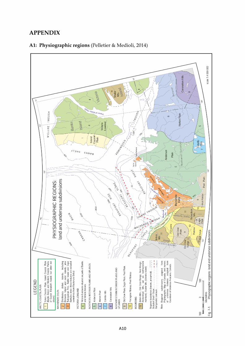
A10

APPENDIX

A1: Physiographic regions (Pelletier & Medioli, 2014)

A2

A2: Overview analytical equipment

Analytical steps Equipment

Centrifuging Centrifuge (Heraeus Multifuge 3S)

Cooking Precision Hot Plate (Präzitherm - Harry Gestigkeit GmbH)

Drying Drying closet (Memmert Drying Oven)

Freeze-Drying Freeze-Dryer (ZIRBUS Sublimator 3-4-5)

Grinding Planetary mill (Fritsch Pulverisette 5)

Shaking

1.

2.

3.

Platform shaker (New Brunswick™ Innova® 2300) Hot plate shaker (Heizplattenschüttler SM 30 AT control – Edmund Bühler GmbH) Overhead shaker (Gerhardt Laboshake)

Splitting Rotary cone sample divider (Fritsch Laborette 27)

Washing Centrifuge (Heraeus cryofuge 8500i)

Weighing

1. 2. 3.

Sartorius MSU224S-100-DU Sartorius micro M3P Mettler Toledo XS105 DualRange Analytical Balance

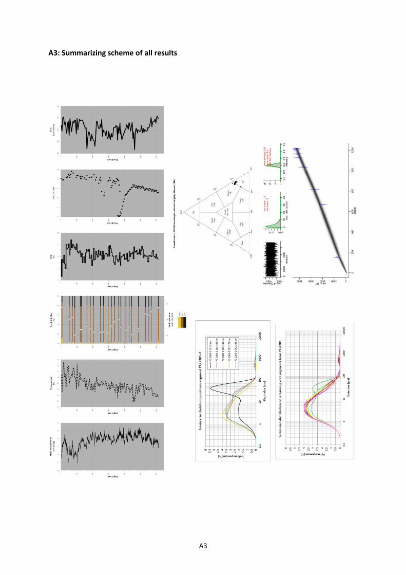
A3

A3: Summarizing scheme of all results

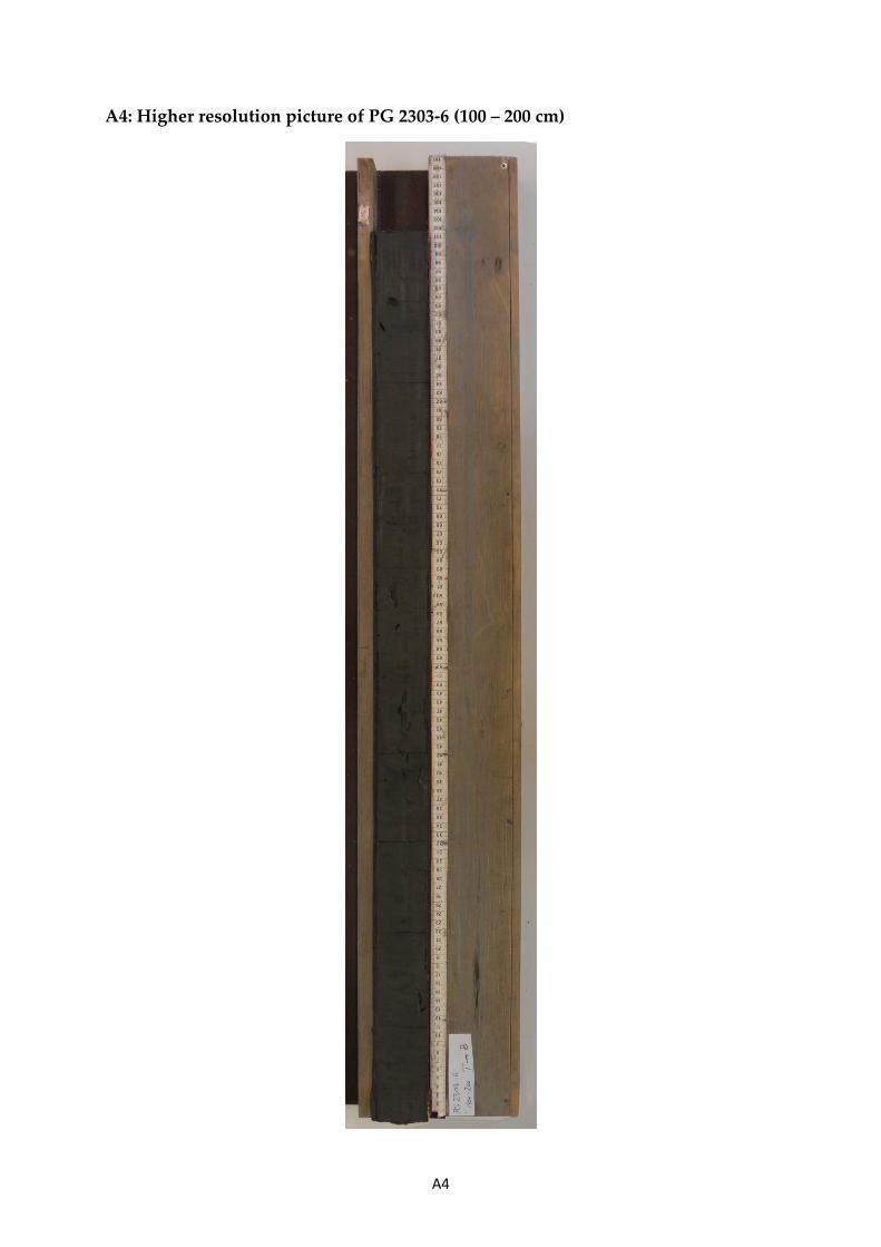
A4

A4: Higher resolution picture of PG 2303-6 (100 – 200 cm)

A5

A5: R-Script for Shepard (1954) sediment triangle

> install.packages("rysgran")

> library("rysgran")

> y <- read.table("PG2303.txt", sep = "\t", header = TRUE)

> without.ID <- y[2:4]

> rysgran.ternary(without.ID, method = "shepard", show.legend = FALSE, main = "Classification of PG2303 according to sediment triangle by Shepard (1954)")

PG2303.txt-file: Sample.ID SAND SILT CLAY PG 2303 - 2 // 12 - 13 cm 11.67088856 75.62796137 12.70115008 PG 2303 - 2 // 102 - 103 cm 4.25819508 74.68605427 21.05575065 PG 2303 - 2 // 142 - 143 cm 3.859650053 74.58789763 21.53860304 PG 2303 - 2 // 172 - 173 cm 1.92644836 73.05768532 25.01586632 PG 2303 - 2 // 242 - 243 cm 3.088709318 75.41880878 21.4924819 PG 2303 - 3 // 42 - 43 cm 2.6737667 76.75584037 20.57039293 PG 2303 - 3 // 112 - 113 cm 3.594496011 78.14733004 18.25817395 PG 2303 - 3 // 152 - 153 cm 2.599197173 77.54398991 19.85681292 PG 2303 - 3 // 192 - 193 cm 2.068778127 78.25422309 19.67699879 PG 2303 - 3 // 282 - 283 cm 2.835717358 76.42028728 20.74399536 PG 2303 - 4 // 51 - 52 cm 2.654488507 77.09723325 20.24827824 PG 2303 - 4 // 111 - 112 cm 2.077058422 76.08591672 21.83702486 PG 2303 - 4 // 151 - 152 cm 3.232597909 74.76595913 22.00144296 PG 2303 - 4 // 191 - 192 cm 3.863705323 75.91990728 20.21253928 PG 2303 - 4 // 271 - 272 cm 2.743109391 75.70590629 21.55098432 PG 2303 - 5 // 17 - 18 cm 3.99934606 75.2255506 20.77510334 PG 2303 - 5 // 107 - 108 cm 1.889269918 77.31767606 20.79305402 PG 2303 - 5 // 147 - 148 cm 2.333800641 76.90676544 20.75943392 PG 2303 - 5 // 177 - 178 cm 1.68619804 77.60960691 20.70419505 PG 2303 - 5 // 267 - 268 cm 3.274026681 77.09483866 19.63113466 PG 2303 - 6 // 23 - 24 cm 2.45455904 75.8713818 21.67405916 PG 2303 - 6 // 113 - 114 cm 3.945796366 73.5115687 22.48723785 PG 2303 - 6 // 153 - 154 cm 4.916356994 73.46149583 21.61444863 PG 2303 - 6 // 183 - 184 cm 4.600859632 74.38269741 20.99490806 PG 2303 - 6 // 273 - 274 cm 4.783550335 73.01434802 22.17053174

A6

A6: R-Script for age-depth model “Bacon”

## setting the working directory for Bacon

> setwd("~/Age Modelling/winBacon_2.2")

## loading Bacon script and environment

> source('Bacon.R')

## selecting the individual core and first run

> Bacon("PG2303", thick = 50, remember = FALSE)

## only showing results every 10 cm

> Bacon("PG2303", thick = 20, remember = FALSE, d.by = 10)

## fitting memory

> Bacon("PG2303", mem.mean = 0.6, mem.strength = 30, thick = 10, remember = FALSE, d.by = 10)

## finding best fit

> Bacon("PG2303", mem.mean = 0.6, mem.strength = 180, acc.shape = 1.2, acc.mean = 3, thick = 10, remember = FALSE, d.by = 5)

## higher resolution

> Bacon("PG2303", acc.shape = 1.2, acc.mean = 3, thick = 5, remember = FALSE, d.by = 5)

## best fit and higher resolution

> Bacon("PG2303", mem.mean = 0.4, mem.strength = 250, acc.shape = 1.2, acc.mean = 3, thick = 5, remember = FALSE, d.by = 5)

## find out the value of a specific depth

> Bacon.hist(0)

## see the modelled age ranges, median and weighted mean ages for each depth of previous Bacon run

> Bacon("PG2303", run=FALSE)

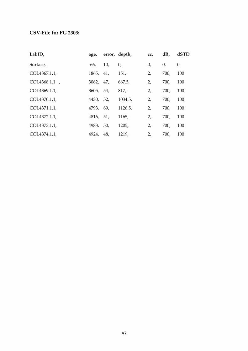
A7

CSV-File for PG 2303:

LabID, age, error, depth, cc, dR, dSTD

Surface, -66, 10, 0, 0, 0, 0

COL4367.1.1, 1865, 41, 151, 2, 700, 100

COL4368.1.1 , 3062, 47, 667.5, 2, 700, 100

COL4369.1.1, 3605, 54, 817, 2, 700, 100

COL4370.1.1, 4430, 52, 1034.5, 2, 700, 100

COL4371.1.1, 4793, 89, 1126.5, 2, 700, 100

COL4372.1.1, 4816, 51, 1165, 2, 700, 100

COL4373.1.1, 4983, 50, 1205, 2, 700, 100

COL4374.1.1, 4924, 48, 1219, 2, 700, 100

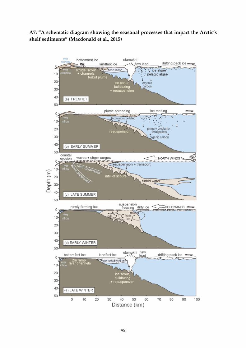
A8

A7: “A schematic diagram showing the seasonal processes that impact the Arctic’s shelf sediments” (Macdonald et al., 2015)

A9

Explanation A7:

(a) Spring freshet: river water overfloods coastal ice and drains down through it, producing strudel scour. The turbid plume is constrained near to shore by the ice cover, and resuspension and coastal erosion are low due to the ice cover. Early primary production and the melting of ice over the middle shelf create a vertical flux of algal organic material.

(b) Early summer: turbid plumes are able to spread farther out on the shelf as ice melts, and the melting ice drops its suspended load. Primary production and secondary production contribute to vertical organic carbon flux.

(c) Late summer: the loss of ice cover from most of the shelf together with winds from the north and warm temperatures lead to rapid coastal erosion, resuspension in the shallow water, and a large near-bottom sediment transport.

(d) Early winter: at this time, there is a high potential for suspension freezing which occurs when cold winds blow over open water at its freezing point. This process may entrain large amounts of mid-shelf sediments into the accumulating ice cover to be exported from the shelf.

(e) Late winter: once an ice cover develops over the shelf, winds no longer produce large waves and resuspension. Landfast ice forms a continuous sheet in the nearshore, grounding at depths less than 2m. The development of rubble and ridges (stamukhi) at the end of the landfast ice produces grounded keels that bulldoze and scour the sediments. Rivers at this time are at their lowest flow and contain relatively few particulates.

A10

Danksagung / Acknowledgment

Zu allererst möchte ich Dr. Michael Fritz, dem Alfred-Wegener-Institut sowie Herrn Prof. Karl-Heinz Feger danken, die es mir ermöglicht haben diese Arbeit zu schreiben. Ohne das Vertrauen in meine Person sowie das unglaubliche Knowhow zu allen fachlichen Fragen und zum Untersuchungsgebiet durch Dr. Fritz und der vollkommenen universitären Unterstützung durch Herrn Prof. Feger wäre diese Masterarbeit in einem mir völlig vorher unbekannten Fachgebiet nie zu Stande gekommen. Dabei muss auch Dr. Lucas Kämpf genannt werden, der im Rahmen dieser Arbeit als Zweitbetreuer eine hervorragende Arbeit geleistet hat.

Weiterhin möchte ich Dyke Scheidemann für die tatkräftige Unterstützung bei der Umsetzung der labortechnischen Methoden danken, da durch seinen Beitrag und Hinweise die Laborarbeit immer im Zeitplan blieb, wenn nicht sogar optimiert wurde. Auch Prof. Dr. Hugues Lantuit sowie der gesamten COPER-Nachwuchsforschergruppe bin ich zum Dank verpflichtet, denn durch ihr Wissen, den regen Austausch von Ideen oder einfach nur den netten Hinweis auf eine Veröffentlichung, wäre diese Arbeit nicht das, was sie jetzt geworden ist. In dem tollen Arbeits- und Forschungsumfeld am Alfred-Wegener-Institut in Potsdam mit großartigen Kollegen ließ sich diese Arbeit um vieles leichter schreiben.

Auch gebührt mein Dank den externen Wissenschaftlern, die diese Arbeit durch ihr Wissen deutlich bereichert haben, vor allem zu nennen sind: Dr. Catalina Gebhardt (AWI Bremerhaven), PD. Dr. Peter Frenzel (Friedrich-Schiller-Universität Jena) und Prof. Dr. Janet Rethemeyer (Universität Köln).

Außerdem möchte ich meiner Familie danken, die mich nicht nur finanziell unterstützt haben, sondern mich auch in allen Lebenslagen angestoßen hatten, über den Tellerrand zu schauen, Tatsache zu hinterfragen und neues Wissen zu akkumulieren, aber einfach auch nur für mich da gewesen sind.

Last but not least, geht mein Dank an meine wunderbare Freundin Maria, die mich in aussichtslosen Situationen motiviert hat, immer ein offenes Ohr für mich hatte, bedingungslos unterstützt und ab und an mich von all dem Trubel richtigerweise abgelenkt hat. Danke dir - ich weiß, warum ich dir mein Herz geschenkt habe.

Diese Arbeit ist nur ein weiterer Baustein auf meinen Weg durch Wissen die Welt zu einem bisschen besseren Ort zu machen. Jedoch sollten wir nie vergessen, dass wir alleine als Menschen dafür verantwortlich sind, wie wir diese Welt gestalten. Ohne Rücksicht auf die Umwelt oder unsere Mitmenschen sind wir zum Scheitern verurteilt. In diesem Sinne hoffe ich, dass uns unsere Menschlichkeit nie verloren geht.

Danke, dass du diese Arbeit gelesen hast.

lateral transport of sediment and organic ... - epic.awi.de · dr. rer. nat lucas kämpf / tu...

Documents