lattice simulations of qcd-like theories at finite baryon...
TRANSCRIPT
Lattice Simulations of QCD-like Theories atFinite Baryon Density
Vom Fachbereich Physikder Technischen Universitat Darmstadt
zur Erlangung des Gradeseines Doktors der Naturwissenschaften
(Dr. rer. nat.)
genehmigte Dissertation vonM.Sc. Philipp Friedrich Scior
aus Groß-Umstadt
Darmstadt 2016D17

Referent: Prof. Dr. Lorenz von SmekalKorreferent: Prof. Dr. Jochen Wambach
Tag der Einreichung: 14.06.2016Tag der Prufung: 13.07.2016
The results of presented in this thesis are solely due to the author. However, parts ofthe thesis have been done in collaboration with other authors. Results for Polyakov loopdistributions and effective potentials in two-color QCD in section 3.1 were obtained incollaboration with David Scheffler, Dominik Smith and Lorenz von Smekal. Parts of thesection are published in [1]. Parts of the results in chapter 4 were obtained togetherwith Bjorn Wellegehausen and Lorenz von Smekal and published in [2, 3]
Zusammenfassung
Die Untersuchung des Phasendiagramms der Quantenchromodynamik (QCD) ist vongroßer Bedeutung zur Beschreibung der Eigenschaften von Neutronensternen oder Schw-erionenkollisionen. Aufgrund des Vorzeichenproblems der Gitter-QCD bei endlichemchemischen Potential benotigen wir effektive Theorien zur Beschreibung der QCD beiendlicher Dichte. Wir verwenden hier dreidimensionale Polyakov-Loop Theorien zurAnalyse der Phasendiagramme QCD-artiger Theorien. Insbesondere untersuchen wirden Fall schwerer Quarks, fur den wir diese effektiven Theorien durch Entwicklung nachinverser Kopplung und inverser Quarkmasse systematisch herleiten und Ordnung furOrdung verbessert konnen. Da die von uns untersuchten QCD-artigen Theorien keinVorzeichenproblem aufweisen, ist es uns moglich, unsere Resultate mit Daten von ab-inito Gittersimulationen dieser Theorien zu vergleichen, um qualitative und quantita-tive Aussagen uber Anwendbarkeit und Gultigkeitsbereich der effektiven Theorien zumachen.Wir starten mit der Herleitung der effektiven Theorien bis zur ubernachsten Ordnungim sogenannten Hoppingparameter, invers zur Quarkmasse, fur Zwei-Farb-QCD und G2-QCD. Dies sind QCD-artige Theorien mit nur zwei anstelle der ublichen drei Farben bzw.mit Eichgruppe G2 anstelle der SU(3) der QCD. Wir beginnen die Analyse der Phasendi-agramme bei endlicher Temperatur, um die effektive Theorie und ihre numerische Imple-mentierung zu testen. Daruber hinaus konnen wir Vorhersagen fur den Deconfinement-Phasenubergang in G2 Yang-Mills-Theorie treffen. Schlussendlich wenden wir uns derkalten und dichten Region der Phasendiagramme zu. Hier beobachten wir, dass dieBaryonendichte abrupt mit dem chemischen Potential fur Quarks an zu wachsen be-ginnt, sobald diese die halbe Diquarkmasse erreicht hat. Bei verschwindender Tem-peratur erwartet man, dass dies in einem Quantenphasenubergang mit Bose-Einstein-Kondensation der Diquarks passiert, der im Gegensatz zum Flussig-Gas-Ubergang derQCD kontinuierlich ist. In der Tat finden wir sehr gute Evidenz dafur, dass die effektivenGittertheorien fur schwere Quarks diesen qualitativen Unterschied zwischen Ubergangenerster und zweiter Ordnung beschreiben konnen. Bei noch großerem chemischen Poten-tial finden wir einen Anstieg des Polyakov-Loop und der Teilchenzahldichte der Quarksbis hin zur charakteristischen Sattigung der jeweiligen Theorie auf einem endlichen Git-ter.
i


Abstract
The exploration of the phase diagram of quantum chromodynamics (QCD) is of greatimportance to describe e.g. the properties of neutron stars or heavy-ion collisions. Due tothe sign problem of lattice QCD at finite chemical potential we need effective theories tostudy QCD at finite density. Here, we will use a three-dimensional Polyakov-loop theoryto study the phase diagrams of QCD-like theories. In particular, we investigate the heavyquark limit of the QCD-like theories where the effective theory can be derived from thefull theory by a combined strong coupling and hopping expansion. This expansion canbe systematically improved order by order. Since there is no sign problem for the QCD-like theories we consider, we can compare our results to data from lattice calculations ofthe full theories to make qualitative and quantitative statements of the effective theory’svalidity.We start by deriving the effective theory up to next-to-next-to leading-oder, in particularfor two-color and G2-QCD where replace the three colors in QCD with only two colorsor respectively replace the gauge group SU(3) of QCD with G2. We will then apply theeffective theory at finite temperature mainly to test the theory and the implementationbut also to make some predictions for the deconfinement phase transition in G2 Yang-Mills theory. Finally, we will turn our attention to the cold and dense regime of the phasediagram where we observe a sharp increase of the baryon density with the quark chemicalpotential µ, when µ reaches half the diquark mass. At vanishing temperature this isexpected to happen in a quantum phase transition with Bose-Einstein-condensation ofdiquarks. In contrast to the liquid-gas transition in QCD, the phase transition to theBose-Einstein condensate is continuous. We find evidence that the effective theories forheavy quarks are able to describe the qualitative difference between first and secondorder phase transitions. For even higher µ we find the rise of the Polyakov loop as wellas the quark number density up to the characteristic saturation of the respective Theoryon a finite lattice.
iii

Contents
1. Introduction 1
2. Theoretical Framework 7
2.1. Lattice Field Theory . . . . . . . . . . . . . . . . . . . . . . . . . . . . . . 7
2.1.1. Monte-Carlo Integration . . . . . . . . . . . . . . . . . . . . . . . . 12
2.2. Two-Color QCD . . . . . . . . . . . . . . . . . . . . . . . . . . . . . . . . 14
2.2.1. Anti-Unitary Symmetries and Dyson’s Classification . . . . . . . . 15
2.2.2. Extended Flavor Symmetry and Spectrum of Two-Color QCD . . 16
2.3. G2-QCD . . . . . . . . . . . . . . . . . . . . . . . . . . . . . . . . . . . . . 17
2.3.1. Symmetries of G2-QCD . . . . . . . . . . . . . . . . . . . . . . . . 18
2.4. Effective Polyakov-Loop Theories . . . . . . . . . . . . . . . . . . . . . . . 20
2.4.1. Yang-Mills Theory . . . . . . . . . . . . . . . . . . . . . . . . . . . 23
2.4.2. Heavy Fermions and Hopping Expansion . . . . . . . . . . . . . . . 30
2.4.3. Corrections to the Effective Fermion Coupling . . . . . . . . . . . 32
2.4.4. Fermions beyond Leading Order . . . . . . . . . . . . . . . . . . . 33
2.4.5. Resummation . . . . . . . . . . . . . . . . . . . . . . . . . . . . . . 41
2.4.6. Effective Action for the Cold and Dense Regime . . . . . . . . . . 42
2.4.7. Effective Action for Nf Flavors . . . . . . . . . . . . . . . . . . . . 42
2.4.8. Mass Scale . . . . . . . . . . . . . . . . . . . . . . . . . . . . . . . 43
2.5. Effective Polyakov-Loop Theory for G2 . . . . . . . . . . . . . . . . . . . . 45
2.5.1. Effective Theory for the G2 Yang-Mills Action . . . . . . . . . . . 45
2.5.2. Leading Order Heavy Fermions for G2 . . . . . . . . . . . . . . . . 46
2.5.3. Kinetic Fermion Determinant for G2 . . . . . . . . . . . . . . . . . 48
3. Results at Finite Temperature 49
3.1. Effective Polyakov-Loop Theory for SU(2) . . . . . . . . . . . . . . . . . . 49
3.1.1. Critical Coupling and Order of the Transition for SU(2) . . . . . . 49
3.1.2. Comparison of Different Action . . . . . . . . . . . . . . . . . . . . 51
3.1.3. Including Dynamical Fermions . . . . . . . . . . . . . . . . . . . . 52
3.2. Effective Polyakov-Loop Theory for G2 QCD . . . . . . . . . . . . . . . . 53
3.2.1. Effective Theory for G2 Yang-Mills Theory . . . . . . . . . . . . . 55
3.2.2. Dynamical Fermions and Critical κ . . . . . . . . . . . . . . . . . . 56
v
Contents
4. Results at Finite Density 594.1. Effective Theory for Two-Color QCD in the Cold and Dense Regime . . . 60
4.1.1. Results for Nf = 1 . . . . . . . . . . . . . . . . . . . . . . . . . . . 634.1.2. Results for Nf = 2 . . . . . . . . . . . . . . . . . . . . . . . . . . . 67
4.2. Effective Theory for G2 QCD at Finite Density . . . . . . . . . . . . . . . 724.2.1. Results . . . . . . . . . . . . . . . . . . . . . . . . . . . . . . . . . 734.2.2. Results outside the Region of Convergence . . . . . . . . . . . . . . 754.2.3. On the Nuclear Liquid-Gas Transition and Bose-Einstein Conden-
sation . . . . . . . . . . . . . . . . . . . . . . . . . . . . . . . . . . 784.2.4. Results for 2 Dimensional G2-QCD . . . . . . . . . . . . . . . . . . 79
5. Summary and Outlook 83
Appendix
A. Basic Facts about Group Representations 89A.1. Higher Dimensional Representations . . . . . . . . . . . . . . . . . . . . . 91A.2. Characters Analysis . . . . . . . . . . . . . . . . . . . . . . . . . . . . . . 91A.3. Invariant Integration on Groups . . . . . . . . . . . . . . . . . . . . . . . . 93
B. Character Expansion for G2 95
C. Parametrization of G2 Elements in Terms of Class-Angles 97
Bibliography 99
Acknowledgment 107
vi

1Introduction
The theoretical framework for the description of particle physics as well as collider andhigh precision experiments is the Standard Model of particle physics. It combines thedescription of Quantum Chromodynamics (QCD) and the electroweak theory, containsall known elementary particles and all forces with the exception of gravity. The StandardModel was and still is highly successful in explaining and predicting experimental datafor about four decades. Though we know, we have to extend the Standard Model to de-scribe neutrino masses, dark matter, dark energy and to incorporate a quantum theoryof gravitation, apart from cosmological observations, there is almost no experimental ev-idence for how and where the Standard Model could go wrong. Even with possible hintsat new physics in the muon’s anomalous magnetic moment [4] or an observed excess inthe diphoton channel around 750 GeV at the Large Hadron Collider [5] the StandardModel is one of the most successful and extensively verified models in physics.
Yet, our physical understanding of the Standard Model remains incomplete. Espe-cially in the case of QCD there are a lot of open questions, and much theoretical andexperimental effort is directed towards answering these questions. The reason for thecomplexity of QCD is its non-Abelian nature, that comes in the form of asymptoticfreedom, which is a blessing and a curse at the same time. Asymptotic freedom wasdiscovered by Wilczek, Politzer and Gross in 1973 [6, 7]. It states that the couplingconstant of QCD is – despite its name – not constant but scale-dependent, leading to anasymptotically vanishing coupling strength as energy increases. On one hand asymptoticfreedom guarantees the renormalizability of QCD, so that it may be valid to the small-est length/ high energy scales, but on the other hand the physics, guaranteeing weakcoupling at high energies, leads to increasing interactions at lower energies until thetheory eventually becomes non-perturbative. At some scale the interaction becomes sostrong, that quarks and gluons – QCDs elementary fields – become locked into hadrons,
1

CHAPTER 1. INTRODUCTION
Temperature
µ
early universe
neutron star cores
ALICE
<ψψ> > 0
SPS
quark−gluon plasma
hadronic fluid
nuclear mattervacuum
RHICCBM
n = 0 n > 0
<ψψ> ∼ 0
<ψψ> > 0
phases ?
quark matter
crossover
CFLB B
superfluid/superconducting
2SC
crossover
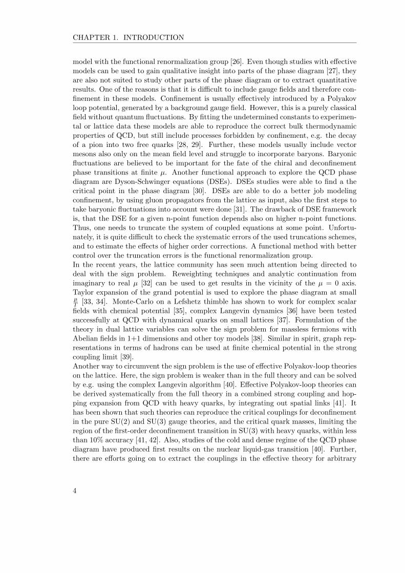
Figure 1.1.: Schematic view of the QCD phase diagram in the T − µ plane. Taken from[8].
like mesons and baryons. This effect is called Confinement and is the reason why wehave never been able to directly observe an isolated quark or a gluon in a detector.Even though quark confinement can be intuitively understood as a concentration of thechromoelectrix flux between two quarks into a flux-tube leading to a linear rising po-tential between the quarks, its underlying physical mechanism is yet unknown [9]. Ingeneral the ultra-violet features of QCD are well understood as perturbation theory isapplicable and able to explain experimental data from e.g. deep in-elastic scatteringto high accuracy [10]. The infrared physics of QCD with important effects like con-finement and dynamical chiral symmetry breaking is much harder to study as we neednon-perturbative methods to do so.The most successful ab-intio method to study the infrared physics of QCD is lattice QCD,where the theory is formulated on a finite Euclidean space-time grid. The discretizationturns the path integral in the generating functional into a finite set of integrals, whichcan be evaluated by using Monte-Carlo methods. Lattice QCD has produced tremen-dous results. The first of these were the reproduction of hadron masses to high accuracy[11]. In the last years it has become possible to extract hadron form factors for electro-magnetic and strong decays [12] or even nucleon scattering phase shifts [13].Despite all these results, there remain areas where there was little progress over the lastyears. Maybe the two most pressing, still standing issues are the nature of confinementand the exploration of the QCD phase diagram.
The knowledge about the thermodynamic properties and the phase structure of stronglyinteracting matter in thermal equilibrium is summarized in the QCD phase diagram. InQCD one is usually interested in the temperature-chemical potential plane of the phasediagram. A conjectured view of the phase diagram is shown in Fig. 1.1. At low tempera-
2

tures T and small chemical potential µ the quarks and gluons are confined into hadrons.Perturbative QCD calculations and heavy ion collisions show that at high temperaturesquarks and gluons are no longer confined into hadrons and form a quark-gluon plasma(QGP) [14]. Parallel to this deconfinement phase transition we expect another phasetransition to happen: We know from hadron spectra that chiral symmetry is brokenat low temperatures, characterized by a finite chiral condensate 〈ψψ〉, while at highertemperatures chiral symmetry is expected to be restored. Even though the phase dia-gram has been studied experimentally and theoretically for many years, we know onlyits most basic properties [15]. It is now well established by lattice QCD that the de-confinement and chiral phase transitions at µ = 0 are analytic cross-overs1 and happenaround 155 MeV [16, 17]. Unfortunately, lattice QCD is unable to provide us with re-sults for the bigger part of the phase diagram as it suffers from the so called fermion signproblem: At finite chemical potential µ > 0 the fermion determinant becomes complexand can not be used as a statistical weight in Monte-Carlo simulations [18]. Perturba-tive QCD is also of limited use for the study of the phase diagram as it is only validfor very high T and µ. There is evidence from model calculations that point to a richphase structure at finite chemical potential, e.g. in Nambu–Jona-Lasinio (NJL) and(Polyakov-)quark-meson model as well as Dyson-Schwinger calculations the deconfine-ment and chiral cross-over transitions will eventually become true phase transitions atfinite chemical potential, that end in a critical point [15]. Inside the hadronic phase wefurther find the nuclear first order liquid-gas transition also ending in a critical point.Both existence and location of this phase transition are well established by experiments[19]. Large Nc arguments suggest that at some point the chiral and deconfinement phasetransitions will move apart from each other and in between emerges a phase of mattercalled quarkyonic [20]. NJL model, quark-meson model and other calculations also sug-gest a region of the phase diagram with inhomogeneous chiral matter characterized by aspatially modulated chiral condensate 〈ψψ〉 [21]. Further, NJL and perturbative QCDstudies suggest color superconducting phases at high chemical potential [22].Experimentally, the phase diagram is explored by heavy-ion collision experiments, e.g.ALICE at CERN [23], experiments at RHIC [24] or planned future experiments at FAIR[19]. Heavy-ion experiments where able to confirm the formation of a quark-gluon plasmaand also to show that the QGP behaves almost like an ideal fluid. Related experiments,like the beam energy scan at RHIC [24] are trying to locate the critical point by analyz-ing fluctuations in specific observables.The properties of the QCD phase diagram at finite µ are not only important for thetheoretical description of heavy-ion collisions, but also for astrophysical observationsconcerning neutron stars. The mass-radius relation and other properties of neutronstars are directly influenced by the QCD equation of state at intermediate to high µ[25].As we already mentioned, most of our knowledge of the QCD phase diagram comesfrom functional methods in low energy effective models of QCD, that share the chiralproperties with QCD but are much simpler, e.g. studies of the (Polyakov-)quark-meson
1Hence, they are not phase transitions in the thermodynamic sense.
3
CHAPTER 1. INTRODUCTION
model with the functional renormalization group [26]. Even though studies with effectivemodels can be used to gain qualitative insight into parts of the phase diagram [27], theyare also not suited to study other parts of the phase diagram or to extract quantitativeresults. One of the reasons is that it is difficult to include gauge fields and therefore con-finement in these models. Confinement is usually effectively introduced by a Polyakovloop potential, generated by a background gauge field. However, this is a purely classicalfield without quantum fluctuations. By fitting the undetermined constants to experimen-tal or lattice data these models are able to reproduce the correct bulk thermodynamicproperties of QCD, but still include processes forbidden by confinement, e.g. the decayof a pion into two free quarks [28, 29]. Further, these models usually include vectormesons also only on the mean field level and struggle to incorporate baryons. Baryonicfluctuations are believed to be important for the fate of the chiral and deconfinementphase transitions at finite µ. Another functional approach to explore the QCD phasediagram are Dyson-Schwinger equations (DSEs). DSEs studies were able to find a thecritical point in the phase diagram [30]. DSEs are able to do a better job modelingconfinement, by using gluon propagators from the lattice as input, also the first steps totake baryonic fluctuations into account were done [31]. The drawback of DSE frameworkis, that the DSE for a given n-point function depends also on higher n-point functions.Thus, one needs to truncate the system of coupled equations at some point. Unfortu-nately, it is quite difficult to check the systematic errors of the used truncations schemes,and to estimate the effects of higher order corrections. A functional method with bettercontrol over the truncation errors is the functional renormalization group.In the recent years, the lattice community has seen much attention being directed todeal with the sign problem. Reweighting techniques and analytic continuation fromimaginary to real µ [32] can be used to get results in the vicinity of the µ = 0 axis.Taylor expansion of the grand potential is used to explore the phase diagram at smallµT [33, 34]. Monte-Carlo on a Lefshetz thimble has shown to work for complex scalarfields with chemical potential [35], complex Langevin dynamics [36] have been testedsuccessfully at QCD with dynamical quarks on small lattices [37]. Formulation of thetheory in dual lattice variables can solve the sign problem for massless fermions withAbelian fields in 1+1 dimensions and other toy models [38]. Similar in spirit, graph rep-resentations in terms of hadrons can be used at finite chemical potential in the strongcoupling limit [39].Another way to circumvent the sign problem is the use of effective Polyakov-loop theorieson the lattice. Here, the sign problem is weaker than in the full theory and can be solvedby e.g. using the complex Langevin algorithm [40]. Effective Polyakov-loop theories canbe derived systematically from the full theory in a combined strong coupling and hop-ping expansion from QCD with heavy quarks, by integrating out spatial links [41]. Ithas been shown that such theories can reproduce the critical couplings for deconfinementin the pure SU(2) and SU(3) gauge theories, and the critical quark masses, limiting theregion of the first-order deconfinement transition in SU(3) with heavy quarks, within lessthan 10% accuracy [41, 42]. Also, studies of the cold and dense regime of the QCD phasediagram have produced first results on the nuclear liquid-gas transition [40]. Further,there are efforts going on to extract the couplings in the effective theory for arbitrary
4

lattice coupling and masses via inverse Monte-Carlo or relative weights methods [43, 44].A totally different way to learn something about genuine features of strongly interactingmatter at finite density is to avoid the sign problem altogether, by studying the phasediagram of QCD-like theories, that share crucial features with QCD but do not havea sign problem. This can be achieved by replacing the gauge group of QCD, namelySU(3), with other gauge groups. The most popular and well studies example is two-colorQCD with the gauge group SU(2). Two-color QCD shares its principle features withQCD, it is asymptotically free and in the infrared it includes confinement and chiralsymmetry breaking. However, there are also important differences: The deconfinementphase transition in the case of pure gauge theory is of 2nd order in contrast to the caseof SU(3) [45]. An additional symmetry between quarks and anti-quarks leads to a mod-ification of the chiral symmetry pattern. Further, the baryons of two-color QCD consistof two quarks, and thus are bosons not fermions, and some of those baryons are alsopseudo-Goldstone bosons from the breaking of chiral symmetry. Still, there has beenand still is much work devoted to the exploration of the phase diagram of two-color QCD[46–49]. Another QCD-like theory without a sign problem is G2-QCD. Here, the gaugegroup is G2, the smallest exceptional Lie group. The deconfinement phase transitionof pure G2 gauge theory is of 1st order, as in SU(3) gauge theory [50]. The spectrumof G2-QCD contains bosonic baryons made out of two quarks but also, like in QCD,fermionic baryons, consisting of three quarks [51]. G2-QCD therefore provides a uniqueopportunity to study a gauge theory with dynamic quarks in the fundamental represen-tation, including fermionic baryons without a sign problem. Of course, one could alsostudy QCD with quarks in the adjoint representation to get a QCD-like theory withfermionic baryons and without a sign problem. However, with adjoint quarks the finiteT deconfinement phase transition will not be a cross-over but a true phase transitionand the chiral and deconfinement phase transitions do not coincide [52]. One particularadvantage of QCD-like theories is that they are an excellent testing ground for effectivetheories, since it is possible to make qualitative and quantitative comparisons betweenresults from effective theories and from lattice simulations at finite density. This forexample has been done in [53, 54], where results from a (Polyakov-)quark-meson modelin a functional renormalization group approach were compared to two-color QCD latticedata.The goal of this thesis is to derive effective Polyakov loop models on the lattice for QCD-like theories with heavy quarks from a combined strong coupling and hopping expansionand get results in the cold and dense regime of the phase diagram that can be comparedto lattice calculations of the full theory. The document will be organized as follows:First, we will give an overview over lattice field theory in general and an introduction inthe two particular QCD-like theories used in this thesis: two-color QCD and G2-QCD.Next, we will discuss the systematic derivation of the effective theory. Following thederivation, we will first give results at finite temperature and compare our results tolattice results form the full theories. We will then give results for the cold and denseregime of the phase diagram and also compare some of our results to results from thefull theory. An overall summary and outlook will be given at the end.
5

2Theoretical Framework
2.1. Lattice Field Theory
Before we start with the main part of this thesis, let us briefly review the basic propertiesof lattice field theory, as it is our approach to calculate the thermodynamic propertiesof QCD-like theories. This introduction serves to establish conventions, notations andto give a background for the non-expert reader.
Gauge theories in the continuum
Let us start, by writing down the Lagrangian of a gauge theory similar to QCD2
L = −1
4F aµνF
aµν + ψa(iγµDµ −m)ψa . (2.1)
The form of the Lagrangian3 is almost fully constrained by locality, Poincare invariance,local gauge invariance and renormalizability. Fermions are represented as Dirac fieldsψ in the fundamental representation of the gauge group. The covariant derivative isdefined as Dµ = ∂µ − giAaµT a, where g is the coupling constant, Aaµ is the gauge field.The field strength tensor is given by
Fµν = − ig
[Dµ, Dν ] = F aµνTa = (∂µA
aν − ∂νAaµ + igfabcAbµA
cν)T a . (2.2)
The T a are the generators of the gauge group, fulfilling
[T a, T b] = ifabcT c , trT aT b =1
2δab .
2Here, similar to QCD, is used in the sense that the matter content of the theory are fermions in thefundamental representation of the gauge group.
3We work with natural units: ~ = c = kB = 1.
7

CHAPTER 2. THEORETICAL FRAMEWORK
The fabc are the structure constants of the given gauge group, for Abelian gauge theoriesall fabc vanish, for non-Abelian theories they are proportional to the self-interactions ofthe gauge fields. Finally, the covariant derivative is contracted with the anti-commutingDirac matrices that are defined by
γµ, γν = 2gµν = 2 diag(1,−1,−1,−1) . (2.3)
Quantization
Up to now all fields are classical, to go to a quantum theory of fields we have to quantizeaccordingly. The standard way in quantum mechanics would be to promote our classicalfields to operators and impose (anti-)commutation relations for our fields. However itturns out, that this is a rather painful way to quantize the theory, as it is impossible toquantize the gauge fields in this way without fixing a gauge [55]. So, instead of promotingour classical fields to operators we will take another way of quantization. We use thepath integral formulation to formulate a quantized theory, here an observable is givenby the expectation value of a given operator
〈O〉 =1
Z
∫DADψDψO eiS[A,ψ,ψ] , (2.4)
Z =
∫DADψDψ eiS[A,ψ,ψ] ,
where S =∫d4xL is the classical action, Z is called the generating functional and we
have to integrate over all field configurations, not only the ones minimizing the classicalaction. Even though we have now quantized our theory, we did not make real progress.It turns out that gauge equivalent field configurations lead to a massive over-counting ofthe physical degrees of freedom and the infinite dimensional integrals over the fields willdiverge. Of course, this is again fixable by choosing a gauge. Yet, gauge fixing for a non-Abelian gauge theory is a non-trivial procedure. In the perturbative regime, this can beachieved by the BRST formalism and the introduction of non-physical auxiliary fields[55]. Unfortunately BRST quantization becomes problematic in the non-perturbativeregime, as the Gribov ambiguity becomes important here.Nevertheless, let us quantize our theory by the path integral formalism. We will see,that because of our chosen regularization, we can just solve the arising integrals by bruteforce and we do not have to care about the finicky matter of gauge fixing at all.
Lattice discretization
To perform the integrations over the gauge fields in eq. (2.4) we have to regulate ourtheory properly. We do this by discretizing space-time to a 4 dimensional hypercubiclattice with finite lattice-spacing a.Before we go into technical details of the discretization, there is one more thing we haveto address. The integrand in eq. (2.4) always comes with the phase factor eiS , hence it
8

2.1. Lattice Field Theory
is highly oscillating. In case of a free field theory one can show that such an integral isonly defined by adding a small imaginary part iε to the action, performing the integraland taking ε→ 0, otherwise the integral does not converge. A convenient way to do this,is by a Wick-rotation of the time direction to imaginary time t → it, this correspondsto changing from Minkowski metric to Euclidean metric and we find
Z =
∫DADψDψ e−SE [A,ψ,ψ] , (2.5)
SE =
∫d4x
(1
4F aµνF
aµν + ψa(iγµDµ +m)ψa
). (2.6)
SE is now the Euclidean action and we do not have to distinguish between co- andcontra-variant indices. Another interesting feature is that the generating functional (2.5)now has the same form as a statistical partition function with the Boltzmann weighte−SE . This allows us to assign a temperature to the system as we identify the inversetemperature of the system β = 1/T with the extend of the compact temporal direction,when we use appropriate boundary conditions
Z =
∫DA
periodic b.c.
∫DψDψ
anti-periodic b.c.
exp
(−∫ β
0dt
∫d3xLE
). (2.7)
The Wick rotation is well defined, and using Euclidean quantum field theory is a wellestablished method when using numerical computations and simulations. The only prob-lem arises when one wants to calculate real-time quantities like e.g. spectral functions.In principle we can do all calculations in the Euclidean framework with imaginary timeand use analytic continuation to translate our results back to Minkowski space with realtime. However as most numerical calculations depend on some discretization in spaceor momentum space one has only a finite set of data points to construct the analyticcontinuation back to real time. This gets problematic, when there are numerical errorsin those data points, as the analytic continuation of a finite set of noisy data points is anill-defined problem. Nevertheless, it is still possible to perform the analytic continuation.It was shown in a functional renormalization group approach, that this can be done in awell defined way on the level of the flow equations [56]. Another well established methodis the maximum entropy method [57].Now let us come back to the lattice discretization. We regulate our Euclidean quantumfield theory by introducing a finite lattice spacing a. We further work in a finite boxwith Nt sites in temporal direction, Ns sites in spatial direction and periodic boundaryconditions. This way, we introduced an UV cutoff by having a shortest length scale a.The finite extend of the lattice L = aNs acts as an IR regulator. Finally, because ofthe finite number of the lattice sites, we only have to perform a finite number of fieldintegrations.
9

CHAPTER 2. THEORETICAL FRAMEWORK
Fermions on the lattice
Let us start our discussion of the discretization of the action with the theory’s fermioncontent. The discretization of the free fermion action is achieved by placing the spinorfields on the discrete lattice sites ψ(x), ψ(x), x ∈ Λ, where we take Λ as the finite setof all sites in our 4d lattice. The x are now discrete 4 vectors and, by discretizing thedifferential symmetrically, the fermion action reads
Sf = a4∑x∈Λ
ψ(x)
(∑µ
γµψ(x+ µ)− ψ(x− µ)
2a+mψ(x)
). (2.8)
The µ denotes a unit vector in the direction µ. We now want to couple the quarksto gluons and therefore have to promote the discretized derivative to a discrete versionof a covariant derivative. This is easiest done by demanding gauge invariance of Sf .The discretized fermion fields transform exactly as the continuum fields under gaugetransformations:
ψ′(x) = Ω(x)ψ(x) , ψ′(x) = ψ(x)Ω†(x) . (2.9)
Is is immediately clear that the mass term is already gauge invariant. However, thederivative terms are not. Consider e.g. the term
ψ(x)ψ(x+ µ)→ ψ′(x)ψ′(x+ µ) = ψ(x)Ω†(x)Ω(x+ µ)ψ(x+ µ) , (2.10)
this is not a gauge invariant quantity. It would be gauge invariant, if we inserted somequantity U(x, x + µ) in between the fermion fields that transforms like U(x, x + µ) →U ′(x, x+ µ) = Ω(x)U(x, x+ µ)Ω†(x+ µ). Luckily, we already know a function with thedesired transformation properties from the continuum formulation of gauge fields, it iscalled a parallel transporter
U(x, y) = P exp
(i
∫C(x,y)
Aµdxµ
), (2.11)
where C(x, y) is a curve between the points x and y and P denotes the path orderingof the exponential. As Aµ is a gauge field, living in the algebra of the gauge group,the parallel transporter is an element of the gauge group itself and thus transforms likeΩ(x)U(x, y)Ω†(y). We will use the notations
U(x, x+ µ) = Uµ(x) = exp[iaAµ(x)] and U−µ(x) = U †(x− µ) (2.12)
and call the Uµ(x) link-variables, as they are directed and can be thought of elementsconnecting two neighboring sites. There is a one-to-one correspondence between Aµ(x)and Uµ(x), hence we will now treat the Uµ(x)’s as our elementary fields. By doing so,our gauge fields are now elements of the gauge group, not the Lie algebra as in thecontinuum formulation.The fermion action reads
Sf = a4∑x∈Λ
ψ(x)
(∑±µ
γµ1
2aUµ(x)ψ(x+ µ) +mψ(x)
). (2.13)
10
2.1. Lattice Field Theory
The above equation is a valid and gauge invariant discretization of the continuum action,however there is a problem. One can easily show that the propagator of free and masslessfermions, discretized in that way, has poles not only at the physical p2 = 0, but also inall corners of the first Brillouin zone resulting in 15 additional poles for 4 dimensions[58]. One way to remove these unphysical doublers is by adding a special term to thefermion action that vanishes in the continuum limit but gives the doublers an additionalmass ∼ 1/a, so that the doublers will decouple from the theory as a→ 0. This is calledthe Wilson fermion formalism and the fermion action reads
Sf = a4∑x,y∈Λ
ψ(x)D(x, y)ψ(y) , (2.14)
where the Wilson Dirac operator is defined as
D(x, y) =
(m+
4
a
)δxy −
1
2a
∑±µ
(1− γµ)Uµ(x)δy,x+µ . (2.15)
The shortcoming of Wilson fermions is that the additional term, giving the extra massto the unphysical doublers, breaks chiral symmetry explicitly. There are other fermiondiscretizations that do not break chiral symmetry, e.g. the staggered fermion formulationbut they will again contain doublers. In fact, the Nilson-Ninoyima theorem states, thereis no local fermion discretization with the right continuum limit that respects chiralsymmetry and has no doublers [59].
Yang-Mills action
We already saw that on the lattice the gauge fields are naturally described by paralleltransporters Uµ(x), living on the links of the lattice. We now have to find a combinationof Us that is gauge invariant and reduces to the standard Yang-Mills action in the limita → 0. Let us start by defining gauge invariant quantities consisting only of gaugefields. The gauge fields transform as Uµ(x)→ U ′µ(x) = Ω(x)Uµ(x)Ω†(x+ µ). Therefore,gauge invariant quantities made of gauge fields will be color traces of closed loops ofgauge fields. The smallest possible loop is made out of four gauge fields and is called aplaquette
Uµν(x) = Uµ(x)Uν(x+ µ)U †(x+ ν)U †ν (x) . (2.16)
These plaquettes are the building blocks of the most simple gauge action, the Wilsongauge action
Sg = − β
Nc
∑x,µ<ν
Re trUµν(x) , (2.17)
with the lattice coupling β = 2Ncg2 . A straight forward calculation shows that Sg has the
right continuum limit
lima→0
Sg =
∫d4x F aµνF
aµν . (2.18)
11
CHAPTER 2. THEORETICAL FRAMEWORK
Continuum limit and renormalization
We were able to show that our chosen lattice discretization has the right continuumlimit, but we still have to answer how to get to the continuum limit in our numericalcalculations. In principle we could just do our calculations with some different valuesa and extrapolate a → 0. However this is problematic, since the gauge action does noteven explicitly depend on a! Furthermore, for the computer a is just a number, so doesa = 0.01 stand for 0.01 fm or 0.01 ly, and is that already close enough to the continuumlimit? So part of the problem is that we simply do not know the scale of the system.From continuum physics we know that to avoid unphysical divergences in loop diagramswe have to renormalize the theory, i.e. the bare parameters of the theory will have anon-trivial dependence on the UV cutoff. This implies that the bare coupling is also adependent g(a). This turns out to be the solution to our problem: from the property ofasymptotic freedom we know that to 1-loop oder we have [60]
g2(a) =1(
113 Nc − 2
3Nf
)log(
Λ2QCD
a2 ). (2.19)
If we invert this we get a(g) and we find limg→0 a = 0. This tells us that we can takethe continuum limit of lattice calculations by computing observables at different latticecouplings β and then take the limit β = 2Nc
g2 →∞. Of course a→ 0 also means that thelattice is shrinking. We therefore have to simultaneously take the thermodynamic limit
β, Nt, Ns →∞ , with T = aNt, L = aNs finite. (2.20)
To remove finite volume effects one has to repeat this a → 0 extrapolation for variousvalues of L and extrapolate to L→∞.
2.1.1. Monte-Carlo Integration
We now take a look a how to do the numerical simulations of QCD-like theories on thelattice. Vacuum or thermal expectation values of any observable in the Euclidean latticeframework are given by
〈O〉 =1
Z
∫[dU ] [dψ] [dψ]O e−S[U,ψ,ψ] , (2.21)
where [dψ] =∏x∈Λ dψx and [dU ] =
∏x∈Λ
∏±4µ=1 dUµ(x) where dUµ(x) is now an invari-
ant measure on the group manifold, called the Haar measure. Solving these integralsnumerically is quite challenging, as the integral are of very high dimensions. An efficientway to perform highly dimensional integrals is Monte-Carlo integration. Here, one ap-proximates the integral by summing over field configurations that are already distributedaccording to the Boltzmann factor e−S
〈O〉 ≈∑
config.s∼e−SO(U , ψ, ψ) . (2.22)
12

2.1. Lattice Field Theory
Since we sum only over a finite number of configurations this introduces a statisticalerror, however one can show that the error will reduce with the number of configurationstaken into account. The only thing we have to do, is to generate configurations U,ψ, ψdistributed according ∼ e−S . This can be done by generating a Markov-Chain with e.g.the Metropolis algorithm as update algorithm or more advanced algorithms like heat-bath or hybrid-Monte-Carlo [58].
Fermion determinant and the sign problem
Taking a look at the partition function of a QCD-like theory, we recognize that the inte-gral in the fermion fields is Gaussian. Therefore, the integration can be done analytically
Z =
∫[dU ] [dψ] [dψ] e−(Sg [U ]+ψD[U ]ψ) ,
=
∫[dU ] e−Sg [U ] det[D(U)] , (2.23)
where D(U) is the Dirac operator of our chosen discretization and its determinant iscalled the fermion determinant. Usually, the fermion determinant is treated numerically,like the gauge action, as a weight factor. This is in principle equivalent to using thefull action as a Boltzmann weight though it is handled differently by the numericalalgorithms, to avoid the Grassmann valued fermion fields on the computer. There is oneimportant constraint on using the fermion determinant (or equivalently the full action)in this way. A well-defined probability weight has to be real and positive! For arbitrarybut well defined actions S this is not necessarily the case. However in most cases we arefortunate and the Dirac operator obeys
γ5Dγ5 = D† ⇒ det[D]∗ = det[γ5Dγ5] = det[D] . (2.24)
This property is called γ5-hermicity and we can indeed check that the relation holds forthe Dirac operator in (2.15). This ensures that for every complex eigenvalue of D, thecomplex conjugate eigenvalue is also part of the spectrum and the determinant is real.It is not necessarily positive, however by taking two degenerate quark flavors we getdet[D]2 > 0.In QCD there is a serious problem when we want to introduce chemical potential for thequarks, to investigate the QCD phase diagram at finite densities. Chemical potential isusually introduced by a modification of the time-like links
U4(x)→ exp(aµ)U4(x) and U−4(x)→ exp(−aµ)U−4(x) . (2.25)
Some quick lines of algebra show that this modification leads to
γ5D(µ)γ5 = D(−µ)† . (2.26)
γ5-hermicity is no longer valid, the fermion determinant is in general complex and weare not able to interpret it as a probability weight at finite µ. Now one could just split
13

CHAPTER 2. THEORETICAL FRAMEWORK
the determinant into absolute value and a complex phase det[D] = eiϕD | det[D]| andinclude the phase into the measured operator. By defining an effective action
Seff = Sg − log(|det[D]|) , (2.27)
we can rewrite (2.21) as
〈O〉 =〈OeiϕD〉Seff
〈eiϕD〉Seff
, (2.28)
which is well-defined also at finite chemical potential. The problem is that this doesnot work numerically. The complex phase eiϕD is rapidly fluctuating in the updateprocess generated by Seff and one needs exponentially many configurations to get reliableexpectation values for observables [61]. The obstacle even gets worse when one increasesthe lattice size. This is called the QCD-sign problem4 at finite density and so far ithas prohibited lattice QCD to fully explore the phase diagram of strongly interactingmatter. One should however note that QCD is not unique in having this property, theQCD sign problem is just one particular example of a so called complex action problemand there are many more systems known, where such problems are present.Recent years have seen much activity in overcoming the sign problem. Taylor expansionof the grand potential in small µ
T , reweighing or canonical approaches [62, 63] haveallowed us to get some information of the phase diagram not to far away from µ = 0.New algorithms for circumventing the sign problem, like complex Langevin or simulationson Lefshetz thimbles [35] have been developed. Other approaches include e.g. switchingto the polymer representation of the fermion determinant [39] or the density of statesmethod [64]. All of the methods stated above were applied successfully to circumvent signproblems for toy models. The most promising results come from the complex Langevinsimulations that were able to get results for QCD at finite chemical potential on smalllattices [37]. So far however, all these methods are not quite there yet. In the nextsections we will discuss a class of QCD-like theories that share many features with QCDbut do not show a sign problem.
2.2. Two-Color QCD
Yang-Mills theory and quantum chromodynamics with only two colors have been andstill are the subjects of extensive research. Two-color QCD has the advantage that it ischeaper to simulate than QCD because it has less color degrees of freedom. Yet, two-color QCD shares a lot of qualitative features with QCD: It is strongly coupled, confiningin the infrared and asymptotically free at high energies. Two-color QCD exhibits a chiralsymmetry breaking pattern very similar to QCD. Moreover, and in contrast to QCD withadjoint matter, the chiral and deconfinement cross-overs at vanishing chemical potentialcoincide [65, 66]. Still there are also important differences, e.g. the deconfinementtransition in the pure gauge theory is a second order phase transition in contrast to the
4Though it is actually the strongly fluctuating complex phase of the fermion determinant, that causesthe problems.
14

2.2. Two-Color QCD
first order transition in QCD. The biggest difference is the fact that the sign problem,that hinders simulations of QCD at finite baryon density, can be easily solved in two-color QCD. Therefore, two-color QCD is an excellent playground to explore the finitedensity phase diagram of a QCD-like theory from first principles. In particular, one canstudy the effects of baryonic degrees of freedom on the phase structure since they areoften omitted in effective models and it can be shown in this case that the phase diagramchanges drastically if baryonic fluctuations are taken into account, e.g. the chiral phasetransition is modified heavily if baryons are taken into account properly [54]. Recentstudies with Dyson-Schwinger equations have shown evidence that this might not be thecase in QCD [31]. Another significant difference to QCD is the fact that in two-colorQCD the baryons, the diquarks, are pseudo Goldstone bosons. One result of this is thatat intermediate chemical potential we expect Bose-Einstein condensation of the diquarks[67]. This is the two-color analog to the nuclear liquid-gas transition in QCD.Two-color QCD is naturally a very rich testing ground for effective theories that mightbe used to explore the QCD phase diagram, as the effective theories can be comparedto first principle lattice calculations in the whole phase diagram.We will now discuss the symmetries of two-color QCD that lead to the absence of a signproblem.
2.2.1. Anti-Unitary Symmetries and Dyson’s Classification
γ5-hermiticity ensures the reality of the fermion determinant only at vanishing chemicalpotential. In contrast to QCD with three colors, there is an additional symmetry intwo-color QCD that ensures the reality of the fermion determinant for all µ.If there is an isometry between the generators of a given representation of the gaugegroup and the complex conjugate representation, like
T a∗ = T T = −ST aS−1 , (2.29)
one is able to construct an anti-unitary symmetry A for the Dirac operator in the givenrepresentation
[A,D] = [SCK,D] = 0 , (2.30)
where C is the charge conjugation operator and complex conjugation is denoted K.Dyson showed that there are only three scenarios for anti-unitary symmetries of D [68].If there is no such anti-unitary symmetry, the representation of the group is complex,i.e. the eigenvalues of D are complex, we associate this case with the Dyson index β = 2.If there is a symmetry with A2 = +1, the complex eigenvalues of D come in complexconjugate pairs and the fermion determinant is always real, but not necessarily positive.We assign this situation with β = 1. The last case is β = 4: There is an anti-unitarysymmetry and A2 = −1, here D has only real eigenvalues and the eigenvalues are two-fold degenerate, resulting in a positive fermion determinant.In fundamental two-color QCD we find S = iσ2, σ2 being the second Pauli matrix, to bean isometry between the generators and for Wilson fermions5 we find T 2 = 1. Therefore
5Without the additional minus sign from C2 the anti-unitary symmetries of staggered fermions areopposite to the continuum formulation or Wilson’s formulation of lattice fermions.
15

CHAPTER 2. THEORETICAL FRAMEWORK
SU(2Nf )
mq > 0 µ > 0
Sp(Nf ) SU(Nf )L × SU(Nf )R × U(1)B
SU(Nf )V × U(1)B〈qq〉 > 0
Sp(Nf/2)V
Figure 2.1.: Patterns of chiral symmetry breaking in two-color QCD with fundamentalquarks.
we can solve the sign problem by taking two degenerate quark flavors with det[D]2 > 0.
2.2.2. Extended Flavor Symmetry and Spectrum of Two-Color QCD
Due to the isometry between the fundamental generators, quarks and anti-quarks belongto equivalent representations and we will find an extended flavor symmetry in this case.Let us start with the kinetic part of the Euclidean quark Lagrangian in the chiral basis
L = ψ /Dψ = ψ†LiσµDµψL − ψ†Riσ†µDµψL , (2.31)
with the transformation
ψR = σ2τ2ψ∗R , ψ∗R = σ2τ2ψR , (2.32)
where σ2 and τ2 are Pauli matrices in spinor and color space, and after some lines ofalgebra we can rewrite the Lagrangian as
L = Ψ†iσµDµΨ , (2.33)
where we introduced the 4NcNf dimensional Nambu-Gorkov spinors
Ψ =
(ψLψR
). (2.34)
Now from eq. (2.33) we can readily see that the Lagrangian is invariant under U(2Nf )chiral symmetry transformations. However just as in the case of QCD the axial U(1)Ais broken by the Adler-Bell-Jackiw anomaly [69, 70] and the symmetry group reducesto SU(2Nf ) which contains the usual chiral SU(Nf )L × SU(Nf )R × U(1)B as a sub-group. And indeed, if we introduce a chemical potential µ > 0, quarks and anti-quarksdo no longer belong to the same representation and the enlarged symmetry group isbroken down to the familiar SU(Nf )L × SU(Nf )R × U(1)B [46]. For vanishing µ, the
16

2.3. G2-QCD
extended SU(2Nf ) can be broken down explicitly by a Dirac mass term for the quarksor spontaneously by a dynamical formation of a chiral condensate 〈qq〉. In this casethe remaining symmetry is given by the compact symplectic group Sp(Nf )6 [71]. Thecoset SU(2Nf )/Sp(Nf ) has dimension Nf (2Nf −1)−1 and we expect as many (pseudo-)Goldstone bosons in the spectrum of the theory. With both, mq > 0 and µ > 0, one isleft with the usual isospin-like and baryon number symmetries, SU(Nf )V × U(1)B. Fortwo-color QCD with two degenerate quark flavors the enlarged flavor symmetry is SU(4)which is spontaneously (explicitly) broken by a chiral condensate (Dirac mass) to Sp(2)resulting in five (pseudo-)Goldstone bosons: the three pions and a scalar diquark/anti-diquark pair. The chiral symmetry breaking pattern is shown in Fig. 2.1
Diquark condensation
Let us start from the vacuum of two-color QCD with two degenerate quark flavors, wherea finite Dirac mass breaks the chiral symmetry explicitly. Still, the quarks and anti-quarks belong to the same representation of the gauge group and all pseudo-Goldstonebosons will have the same mass mπ. By dialing up chemical potential the excitationenergy of the diquark will decrease like ωd = mπ − 2µ, the excitation energy of the anti-diquark will increase, while the pion energy will stay unchanged. At a critical µc = mπ
2we can excite diquarks essentially for free and a Bose-Einstein condensate of diquarkswill form. There is exactly one way to write down a gauge invariant scalar diquarkcondensate
〈qq〉 = 〈qTCγ5T2τ2q〉 . (2.35)
The formation of the diquark condensate again restricts the remaining chiral symmetry.In the presence of a 〈qq〉 condensate the remainder of the chiral symmetry is given bySp(Nf/2)V .
2.3. G2-QCD
We will now turn our attention to a QCD-like theory, where we replace the gauge groupSU(3) by the group G2. G2 is the smallest of the exceptional Lie groups in Weyl’s classi-fication of classical Lie groups. One particular definition is that G2 is the automorphismgroup of the octonions algebra, or equivalently, the subgroup of SO(7) that obeys
cabc = cdefUdaUebUfc , (2.36)
cabc =1√3ψabc a, b, c ∈ 1, 2, 3, 4, 5, 6, 7 ,
where ψabc is the totally antisymmetric octonionic tensor defined by [72]
ψ123 = ψ147 = ψ165 = ψ246 = ψ257 = ψ354 = ψ367 = 1 . (2.37)
6Since the anti-unitary symmetry is different for staggered quarks, we also find a different chiral sym-metry breaking pattern. Here, chiral symmetry gets broken down spontaneously to O(2Nf )
17
CHAPTER 2. THEORETICAL FRAMEWORK
This amounts to seven non-trivial constraints, reducing the 21 generators of SO(7) tothe 14 generators of G2. G2 has rank 2 and includes SU(3) as a subgroup
G2/SU(3) ∼ SO(7)/SO(6) ∼ S6 . (2.38)
G2 has two fundamental representations a 7-dimensional and a 14-dimensional, theycarry the Dynkin labels
(7) = [1, 0] , (14) = [0, 1] , (2.39)
The 14-dimensional fundamental representation is also the adjoint representation whichis an unfamiliar feature coming from SU(N) gauge theories. G2 gauge theory was firstinvestigated by Pepe and Wiese [50] and was introduced to clarify the influence of thegroup-center on deconfinement. It was shown that G2 Yang-Mills theory exhibits a firstorder phase transition even though it has a trivial center.
2.3.1. Symmetries of G2-QCD
There is another feature of G2 that makes it very interesting to use as a gauge group ofa QCD-like theory. As a subgroup of SO(7), G2 is real, i.e. all representations of G2
are real and there is a trivial isometry between the generators of a given representationand its complex conjugate, leading to an anti-unitary symmetry for the Dirac operator[A,D] = 0 with A2 = −1. That implies β = 4 for the Dirac operator and there is no signproblem. The reality of G2 also has important consequences on the fermion content ofthe theory. Let us start this discussion with the G2-QCD action with Nf quark flavorsin the continuum
S =
∫d4x
(−1
4FµνF
µν + ψi(iγµDµ −m)ψi
), (2.40)
where summation over the flavor index i = 1, . . . , Nf is implied and color indices aresuppressed. The matter part of the Lagrangian transforms under charge conjugation(up to irrelevant boundary terms) as
LC = ψC(iγµ(∂µ − gAµ)−m)ψC ,
= ψ(iγµ(∂µ + gATµ )−m)ψ . (2.41)
(2.42)
That is, ifATµ = −Aµ = −AaµT a , (2.43)
then the Lagrangian is invariant under charge conjugation. Since every representationof G2 is real, eq. (2.43) holds and we can replace the Nf Dirac spinors by 2Nf Majoranaspinors
S =
∫d4x
(−1
4FµνF
µν + λi(iγµDµ −m)λi
), (2.44)
with λC = CλT . The connection between the Majorana and Dirac spinors is given byλ = (χ, η) and ψ = χ+ iη.
18
2.3. G2-QCD
SU(2Nf )L=R∗ × Z(2)B
mq > 0 µ > 0
SO(2Nf )V × Z(2)B SU(Nf )L × SU(Nf )R × U(1)B
SU(Nf )V × U(1)B
Figure 2.2.: Patterns of chiral symmetry breaking in G2-QCD.
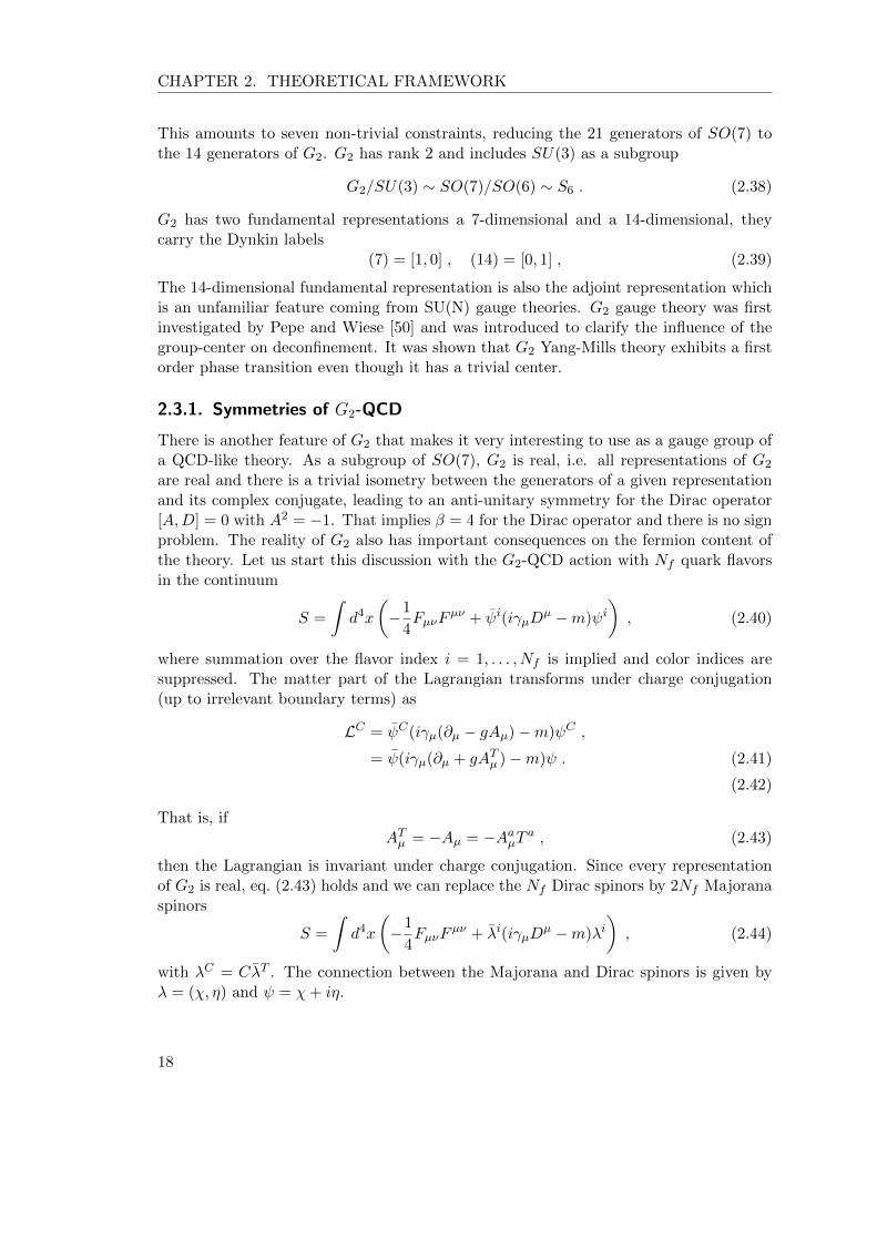
Now, what is the chiral symmetry and the breaking patterns of G2-QCD? Eq. (2.44)suggest a U(2Nf ) symmetry. This is broken down by the axial anomaly toSU(2Nf )L=R∗ × Z(2)B, which looks unfamiliar because we consider Majorana fermions.Because of the Majorana condition, we are not free to transform the left- and right-handed components independently. In fact, the Majorana condition requires L = R∗ [73].In the same way the U(1)B = U(1)L=R is reduced to U(1)B = U(1)L=R=R∗ = Z(2)B.As we cannot distinguish between quarks and anti-quarks, the U(1)B baryon numbersymmetry is reduced to Z(2)B that distinguishes between states with even and oddnumbers of quarks. As in ordinary QCD, the introduction of a finite Dirac mass or achiral condensate breaks the axial part of the SU(2Nf )L=R∗ × Z(2)B and we are left withthe vector part of the symmetry SU(2Nf )L=R=R∗ × Z(2)B = SO(2Nf )L=R × Z(2)B,leading to 4N2
f − 1 − Nf (2Nf − 1) = Nf (2Nf + 1) − 1 Goldstone bosons. Alreadyfor Nf = 1 we will find (pseudo-)Goldstone bosons in our spectrum: a scalar and apseudo-scalar diquark
d(0+) = χγ5η = ψCγ5ψ − ψγ5ψC
d(0−) =1√2
(χγ5χ− ηγ5η) = ψCγ5ψ + ψγ5ψC .
The introduction of chemical potential corresponds to an off-diagonal term in the La-grangian with Majorana fields
ψ(i /D −m+ iγ0µ)ψ =(χ, η
)(i /D −m iγ0µ−iγ0µ i /D −m
)(χη
), (2.45)
violating the Majorana decomposition and we are left with the usual SU(Nf )L×SU(Nf )R×U(1)B. The chiral symmetry breaking pattern is summarized in Fig. 2.2.Now let us analyze the expected colorless spectrum of the theory by decomposing the
19

CHAPTER 2. THEORETICAL FRAMEWORK
tensor products of the fundamental representations
(7)⊗ (7) = (1)⊕ (7)⊕ (14)⊕ (27)
(7)⊗ (7)⊗ (7) = (1)⊕ 4 · (7)⊕ 2 · (14)⊕ 3 · (27)⊕ . . . ,(14)⊗ (14) = (1)⊕ (14)⊕ (27)⊕ . . . , (2.46)
(14)⊗ (14)⊗ (14) = (1)⊕ (7)⊕ 5 · (14)⊕ . . . ,(7)⊗ (14)⊗ (14)⊗ (14) = (1) . . . .
We find a rich spectrum containing glueballs, mesons and baryons. From the first twolines in (2.46) we can conclude that the spectrum of G2 contains two kinds of baryons:bosonic diquarks as in two-color QCD and fermionic three-quark states as in QCD. Wealready saw that the scalar diquarks are Goldstone modes of the theory. In contrast toother QCD-like theories with matter in the fundamental representation, we can also findhybrid states that consist of quarks and gluons. The existence of those lead to stringbreaking already in G2 Yang-Mills theory.Since there is no sign problem in G2-QCD, Lattice Monte-Carlo techniques allows usto explore the phase diagram of a QCD-like theory with fermionic baryons from firstprinciples, i.e. the investigation of a nuclear liquid-gas transition, that is also present inQCD, or the search for a critical point in the phase digram without the need of effectivemodels.
2.4. Effective Polyakov-Loop Theories
In this work we will make extensive use of effective theories for QCD-like theories thatuse the so called Polyakov loops as degrees of freedom. Let us first discuss the role ofthe Polyakov loop in the case of pure gauge theory. The Polyakov loop is defined as
L(~x) = tr
t=Nt∏t=1
U0(~x, t) . (2.47)
It thus is the trace of a loop holonomy of gauge links that winds around the lattice inthe compact, periodic time direction. Under a global center transformation U0(~x, t0)→zU0(~x, t0) the Polyakov loop transforms according to
L(~x)→ zL(~x) . (2.48)
Therefore, the Polyakov loop acts as an order parameter for the spontaneous breaking ofcenter symmetry. One also finds that the expectation value of the Polyakov loop probesthe screening properties of a static color test charge. In particular the difference in thefree energy Fq(T ) of a gauge theory with and without a single color test charge is
e−Fq(T )/T ∝ |〈L〉| . (2.49)
Thus the Polyakov loop also acts as an order parameter for confinement. When thevacuum is center symmetric we have |〈L〉| = 0 and the free energy for putting a single
20
2.4. Effective Polyakov-Loop Theories
quark into the system is infinite. When center symmetry is spontaneously broken wehave |〈L〉| > 0 and the free energy of a single quark in the systems becomes finite.Now we know that the Polyakov loop is an order parameter for the deconfinement phasetransition in the pure gauge theory. That alone already justifies a phenomenologicalmodel with the Polyakov loop as the degree of freedom in a Ginzburg-Landau theory forthe deconfinement phase transition. Note, that this is a phenomenological argument thatis only valid on mean-field level. However, the Svetitsky-Yaffe conjecture [74] states thatif one integrates out all spatial links in a d+1 dimensional SU(N) gauge theory, one endsup with a d dimensional SU(N) Polyakov-loop theory with only short-range interactions.If the phase transition of the original gauge theory is of 2nd order, the Polyakov-looptheory and the underlying d+1 dimensional gauge theory belong to the same universalityclass and we can compute the order of the finite temperature confinement-deconfinementphase transition and the critical exponents with the effective Polyakov-loop theory whichis easier to handle numerically. Even though the arguments by Svetitsky and Yaffe areonly conjectures, there is reasonable evidence for these conjectures to be true. Highprecision analysis of 3+1 dimensional SU(2) gauge theory shows that it belongs to the3d Ising universality class [75] according to the Svetitsky-Yaffe conjecture. Also datafor SU(2) and SU(3) gauge theory in 2+1 dimensions shows that these gauge theoriesbelong to the same universality classes as the according spin models [76].Now, strictly speaking the universality arguments of Svetitsky and Yaffe are only validfor theories with a 2nd order phase transition where the correlation length of the sys-tem ξ diverges. SU(3) Yang-Mills theory in 3+1 dimensions shows a weak 1st orderconfinement-deconfinement phase transition. Thus, an effective Polyakov-loop theorycan only provide an effective description of the phase transition because the correlationlength ξ is finite and the differences in the microscopic physics will show up at somescale. Nevertheless there are many efforts to explore SU(3) gauge theories by the meansof effective SU(3) or Z3 spin models in the literature [77–79].In the past effective Polyakov loop models were popular to determine properties likee.g. the order of the phase transition of the underlying d+1 dimensional gauge theoryvia the Svetitsky-Yaffe conjecture. When it became numerically feasible to simulate thefull theory people lost interest in effective Polyakov-loop theories. The most importantreason for that might be, that QCD in not only pure SU(3) gauge theory but there arealso dynamical fermions. These dynamical fermions break center symmetry explicitly.Therefore, in QCD and QCD-like theories with fundamental fermions we do not have areal phase transition but a smooth cross-over between the confined and the deconfinedphase. Since there is no real phase transition if we include dynamical fermions, we canno longer rely on universality arguments. And it is quite unclear how to relate the cross-over deconfinement transition in QCD to the one in an effective Polyakov loop model.In the last decade effective Polyakov-loop theories had quite a resurgence. Maybe themost important reason for that is the sign problem of QCD at finite chemical poten-tial. There has been a lot of effort to solve the sign problem of QCD, see section 2.1.1,however, all those methods so far work only for theories simpler than QCD. EffectivePolyakov-loop theories are one class of theories, where the sign problem at finite chem-ical potential is solvable by e.g. the complex Langevin method. Therefore, they are an
21

CHAPTER 2. THEORETICAL FRAMEWORK
important testing ground for the algorithms. Further, as Polyakov-loop theories are stilleffective theories for QCD, one can hope that we might be able to extract informationabout the properties of QCD at finite density.Now let us take a look at how to actually derive an effective Polyakov-loop theory. Ingeneral the effective action for the Polyakov-loop theory is defined by
exp(−Seff[L]) =
∫DUδ(L− L[U ]) exp(−S[U ]) . (2.50)
The only task we have to do is to evaluate the integral. However for most theories this isa quite indomitable task. The good thing is, that we know the basic form of the effectiveaction just from symmetry arguments
Seff =∑~x~y
L~xK(2)(~x, ~y)L†~y +
∑~w~x~y~z
L~wL~xK(4)(~w, ~x, ~y, ~z)L†~yL
†~z + . . .
+∑~x
(h(1)L~x + h(1)L†~x
)+ . . . . (2.51)
The first terms contain only even numbers of Polyakov loops and respect center sym-metry. Their origin lies in the Yang-Mills part of the underlying QCD-like theory. Thelatter terms contain odd numbers of Polyakov loops and break center symmetry explic-itly. Those terms originate in the fermonic part of the action7. Note that eq. (2.51)contains infinitely many terms. Not only with arbitrary numbers of Polyakov loops inthe fundamental representation of the gauge group but also with loops in the adjoint oreven higher representations [80][43].Now we know the general form of the effective action. What we now need to do is to de-termine the form of the kernels K(2n), they will in general depend on the lattice couplingβ, the temperature T and the fermion mass m8, and the form of the center-breakingcouplings h(n), they will also depend on β, T and m. There are several methods how todetermine the effective kernels and couplings. One method is to find the effective kernelsK(2n) via inverse Monte-Carlo calculations [81] [43]. Here one generates an ensemble ofgauge configurations with the underlying gauge theory. One uses these configurationsto calculate the expectation values of an appropriate set of operators 〈X〉. Now one canlook at the Dyson-Schwinger equations for the effective theory. They will depend on thekernels K(2n) and some coefficients. It turns out that those coefficients are given by theexpectation values of our set of operators 〈X〉 that we have computed by Monte-Carlosimulations. So now one has a set of equations for the kernels or respectively for theeffective couplings of the effective Polyakov-loop theory.Another way to compute the effective kernels and couplings is the relative weights
7The fermionic part will also generate terms that contain even numbers of Polyakov loops. Those termsrespect center symmetry. However, all terms that do not respect center symmetry will come fromthe fermionic part not from the Yang-Mills part of the action
8Since the terms containing the kernels K(2n) originate in the Yang-Mills part of the action we wouldnot expect the kernels to depend on the fermion mass. However we will see later, that non-windingfermion loops can be absorbed in the Yang-Mills action and thus lead to mass depended correctionsof the lattice coupling β
22

2.4. Effective Polyakov-Loop Theories
method [44, 82, 83]. Here one uses a slight modification of a standard Monte-Carloalgorithm for the full gauge theory. The algorithm is chosen such that the configu-rations of the untraced Polykov loop is fixed. This is done for some set of differentPolyakov loop configurations. This way, one can calculate derivatives of the effectivePolyakov loop action in the configuration space of our effective theory. When one usesan ansatz for the spatial distribution of the values of the Polyakov loop one can use thederivatives of the effective action to construct the effective kernels and couplings of theeffective theory.The methods described above have been applied very successfully, e.g. Polyakov loopcorrelators computed by an effective theory via the relative weights method match thecorrelators from the full gauge theory perfectly well over a large range of values for βeven in the deconfined phase [44]. However, all methods described above need somewhatheuristic truncations and ansatzes for the effective action. Further, so far none of thosemethods were able to include dynamical fermions in the effective theory. Thus we willtake a different approach to derive our effective action from the full QCD-like theory.The method we will use relies on a combined strong coupling and hopping expansionand was developed by Langelage, Philipsen et al.[40–42, 84]. In this way we are ableto derive the effective action for the Polyakov-loop theory from the underlying gaugetheory in a systematic way and we are in principle able to improve the effective actionorder by order. In the following sections we will see how to derive the effective actionfrom the full QCD-like theory. We will start with Yang-Mills theory and later we willsee how to add dynamical fermions to the theory.
2.4.1. Yang-Mills Theory
Consider the partition function of the non-Abelian gauge field action
Z =
∫[dU0][dUi] exp
[β
2Nc
∑p
(trUp + trU †p)
], β =
2N
g2. (2.52)
In order to arrive at an effective Polyakov-loop theory we integrate out the spatial degreesof freedom of the gauge fields.
Z =
∫[dU0] exp[−Seff ] ,
−Seff = ln
∫[dUi] exp
[β
2Nc
∑p
(trUp + trU †p)
], (2.53)
≡+ λ1S1 + λ2S2 + ... .
The effective couplings λn = λn(β,Nt) are arranged in increasing order in β, thus theλn get neglectable the higher n is. Using the character expansion of the gauge group(details of group representations and character analysis may be found in appendix A),
23
CHAPTER 2. THEORETICAL FRAMEWORK
we can write the effective action in (2.53) as
− Seff = ln
∫[dUi]
∏p
1 +∑j 6=0
djaj(β)χj(Up)
. (2.54)
The sum goes over all irreducible representations with dimension dj and character χj .Since we are interested in expectation values rather than the free energy, we droppeda constant factor (depending only on β and the lattice volume. See also [61]). For thegauge group SU(2) the explicit expressions of the expansion coefficients aj(β) are givenby
aj(β) =I2j+1(β)
I1(β)=
β2j
22j(2j + 1)!+O(β2j+2) , (2.55)
Where the In are modified Bessel functions. For more complicated gauge groups, e.g.SU(3) the aj(β) cannot be written down in a closed form, see appendix A.2. If oneexpands the product in eq. (2.54) one generates terms that contain products of plaquettesin different, non-trivial representations
drp1arp1χrp1 (Up1) · drp2arp2χrp2 (Up2) · · · . (2.56)
Plaquettes that do not appear in a particular term are in the trivial representation.Now we can think of term like the one in eq. (2.56) as a graph. In general an arbitrarygraph will consist of disjoint pieces. We can decompose every such graph into connectedpieces, those are called Polymers X. The contribution of such a Polymer to the effectiveaction, after integrating out the spatial degrees of freedom, is called the activity Φ ofthe Polymer. In the following we will restrict ourselves to plaquettes in the fundamentalrepresentation, since higher dimensional representations contribute to a higher order inβ. For simplicity we will call a1/2 = u. By using the the moment-cumulant formalism andcluster expansion one can show that the contributions to the effective action are givenby the activities of clusters C which consist of a connected set of Polymers [61, 85]. Theeffective action then reads
−Seff =∑
C=(Xnll )
a(C)∏l
Φ(Xl;Wj)nl , (2.57)
Φ(Xl;Wj) =
∫[dUi]
∏p∈Xl
drparpχrp(Up) .
The combinatorial factor a(C) depends on how the polymers Xl are connected in thecluster, and is one for a single polymer [61]. Since we only integrate over spatial degreesof freedom the activities Φ still depend on the Polyakov line variables Wj . To work out,which kinds of Polymers Xl do contribute to the cluster expansion and to calculate theiractivities Φ(Xl) we need to perform group integrals of the type∫
dUχr1(V1U) · ... · χrn(VnU) . (2.58)
24

2.4. Effective Polyakov-Loop Theories
In principle one needs to calculate the Clebsch-Gordan decomposition of the product inthe equation above. If the resulting decomposition does not contain the trivial represen-tation the integral vanishes (for more details see appendix A.3), since:∫
dUχr(U) = δr,0 . (2.59)
Important consequences are:
1. contributing Polymers do not have spatial boundaries. If they had a spatial bound-ary we would have at least one link, where we had an integral of the form:∫
dUχr(V1U)χ0(V2U†) = 0 , (2.60)
since any plaquette that is not part of the Polymer is regarded as a plaquette in thetrivial representation. The integral vanishes, because the Clebsch-Gordan decom-position between any non-trivial and the trivial representation does not containthe trivial representation.
2. if precisely two plaquettes with representations r and r′ meet in a link, we musthave r = r′ or r∗ = r′ depending on the plaquettes’ orientations:∫
dUχr(V1U)χr′(V2U†) = δr,r′
1
drχr(V1V2) . (2.61)
Leading Order Effective Action
Up to now, our discussion about the derivation of the effective action was completelygeneral. We now specialize on the case of the gauge group SU(2), since the specific formof the effective action depends on the properties of the particular gauge group. Lateron we will also show how the effective action for the gauge group G2 will look like.Following the rules of the strong coupling expansion, and integrating over the Ui we caneasily see, that the only graphs yielding a non-constant contribution are those, that closearound the lattice in time direction. Graphs, that do not wind around the time directionof the lattice only produce constant terms which drop out in expectation values. Thefirst graph with a non-trivial contribution thus is a chain of time-like plaquettes windingaround the torus in time direction (Figure 2.3). The contribution from this graph isgiven by
λ1S1 = uNt∑<~x~y>
L~xL~y , (2.62)
where the summation is over nearest neighbors. To get to this result one has to succes-sively apply (2.61). The last step is the integration of the link at the edge of the lattice,one can use [58]: ∫
dUU(r)ab (U †)
(r)cd =
1
drδa,dδb,c , (2.63)
where U (r) is an SU(2) element in the representation r. Improvement of λ1 by includinggraphs with decorations is a non-trivial procedure explained in the next section.
25

CHAPTER 2. THEORETICAL FRAMEWORK
LiLj
Figure 2.3.: First graph with a nontrivial contribution after spatial integration for alattice with temporal extent Nt = 4. Four plaquettes in the fundamental representationlead to an interaction term involving two adjacent fundamental Polyakov loops L~x andL~y.
Corrections From Decorations
At leading order we found λ1 = uNt . However there are contributing clusters that aretopologically equivalent to the leading order result, i.e. those contributions will leadto the same effective action but with additional plaquettes that will lead to a higherorder in u. Clusters resulting in corrections to λ1 will consist of one large polymerΞ winding around the time direction of the lattice and some additional polymers Xi
attached to Ξ. Clusters consisting of several large polymers lead to corrections of orderβNt and will be neglected. Large polymers Ξ are constructed from the leading orderdiagram by adding some decorations to it. One can calculate the corrections to the LOeffective action or respectively the LO λ1 by taking the leading order diagram Ξ0 andcutting out a connected set of plaquettes. Now take a rigid configuration of plaquettesas decoration and plug it into the hole, such that a new admissible large polymer Ξoriginates [85]. The other polymers Xi of the cluster C are directly attached to Ξ. In
Figure 2.4.: Some polymers with decorations
order to examine, how these new clusters contribute, we shall perform a second moment-cumulant transformation. For this purpose we define two new types of polymers. Wecall a polymer of type X, if it is connected to Ξ and does not touch any decorations.Polymers of type Y are decorations with or without other polymers attached to them.Now the cluster C under consideration may be viewed at as composed of polymers Xi
and Yi touching a band of plaquettes Ξ0. The product of all activities in C can beexpressed as
Φ(Ξ0)∏i
Φ(Xi)∏k
Φ(Yk) , Φ(Ξ0) = uNtLiLj , (2.64)
26
2.4. Effective Polyakov-Loop Theories
with well-defined activities Φ(Yk). As with a usual cluster expansion we write:
λ1S1 = S1uNt
1 +∑m>0
∑W1,...,Wm
1
m!〈W1, ...,Wm〉
m∏i
Φ(Wi)
, (2.65)
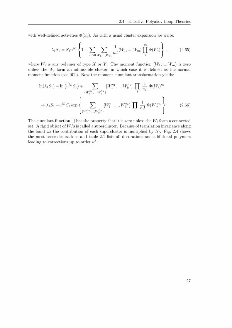
where Wi is any polymer of type X or Y . The moment function 〈W1, ...,Wm〉 is zerounless the Wi form an admissible cluster, in which case it is defined as the normalmoment function (see [61]). Now the moment-cumulant transformation yields:
ln(λ1S1) = ln(uNtS1
)+
∑(W
n11 ,...,W
nkk )
[Wn11 , ...,Wnk
k ]∏i
1
ni!Φ(Wi)
ni ,
⇒ λ1S1 =uNtS1 exp
∑
(Wn11 ,...,W
nkk )
[Wn11 , ...,Wnk
k ]∏i
1
ni!Φ(Wi)
ni
. (2.66)
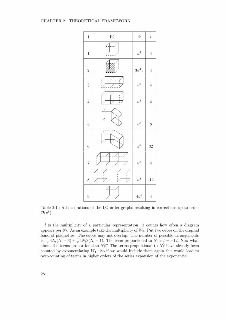
The cumulant function [ ] has the property that it is zero unless the Wi form a connectedset. A rigid object ofWi’s is called a supercluster. Because of translation invariance alongthe band Ξ0 the contribution of each supercluster is multiplied by Nt. Fig. 2.4 showsthe most basic decorations and table 2.1 lists all decorations and additional polymersleading to corrections up to order u8.
27
CHAPTER 2. THEORETICAL FRAMEWORK
i Wi Φ l
1 u4 4
2 3u4v 4
3 u6 4
4 u8 4
5 u8 8
6 u8 32
7 u8 4
8 u8 -12
9 4u6 4
Table 2.1.: All decorations of the LO-order graphs resulting in corrections up to orderO(u8).
l is the multiplicity of a particular representation, it counts how often a diagramappears per Nt. As an example take the multiplicity of W8: Put two cubes on the originalband of plaquettes. The cubes may not overlap. The number of possible arrangementsis: 1
2!4Nt(Nt − 3) + 12!4Nt3(Nt − 1). The term proportional to Nt is l = −12. Now what
about the terms proportional to N2t ? The terms proportional tu N2
t have already beencounted by exponentiating W1. So if we would include them again this would lead toover-counting of terms in higher orders of the series expansion of the exponential.
28

2.4. Effective Polyakov-Loop Theories
The correction W9 is actually a cluster consisting of a cube and the LO diagram, havingone plaquette in common. Therefore we get a combinatoric factor a(C) = −1, whenadding this correction.Further in W2 the gray plaquette is a plaquette in the adjoint representation leading tothe factor v = a1(β). We can use the following relation to get the right order in u of thecorrection:
v =2
3u2 +
2
9u4 +
16
135u6 + ... (2.67)
This is enough to calculate the corrections of Langelage et al. [42, 86]:
λ1(u, 2) = u2 exp
[2
(4u4 − 8u6 +
134
3u8 − 49044
405u10
)], (2.68)
λ1(u, 3) = u3 exp
[3
(4u4 − 4u6 +
128
3u8 − 36044
405u10 +
751744
405u12
)],
λ1(u, 4) = u4 exp
[4
(4u4 − 4u6 +
140
3u8 − 37664
405u10 +
3541576
1215u12
)],
λ1(u,Nt ≥ 5) = uNt exp
[Nt
(4u4 − 4u6 +
140
3u8 − 36044
405u10 +
863524
1215u12
)].
Higher Order Terms
There also occur terms of higher order in u that lead to a different form of the effectiveaction, e.g. terms with a larger number of Polyakov loops involved, or an interaction ofloops with distance greater than one, and loops in higher dimensional representations.The simplest higher order corrections come from Polyakov loops winding several timesaround the lattice. It is an easy task to sum up their contributions:∑
<~x~y>
(λ1L~xL~y −
1
2(λ1L~xL~y)
2 +1
3(λ1L~xL~y)
3 − ...)
=∑<~x~y>
ln(1 + λ1L~xL~y) . (2.69)
The coefficients of this series are given by the combinatorial factors a(C) from (2.57).Now consider corrections coming from Polyakov loops with distance greater than one.The leading non-zero contribution comes from an L-shaped graph with a decoration oftwo additional plaquettes (Figure 2.5). It is given by
λ2S2 = Nt(Nt − 1)uNt+2∑[~x~y]
L~xL~y , (2.70)
and we have to sum over all loops with a distance of√
2a. Calculations by Langelageet al. [42] have shown that it is sufficient to use an effective action where we includeresummation of loops winding around the lattice several times but without terms likeλ2S2. The partition function of our effective theory is then given by
Z =
∫[dU0]
∏<~x~y>
[1 + λ1L~xL~y
]. (2.71)
29
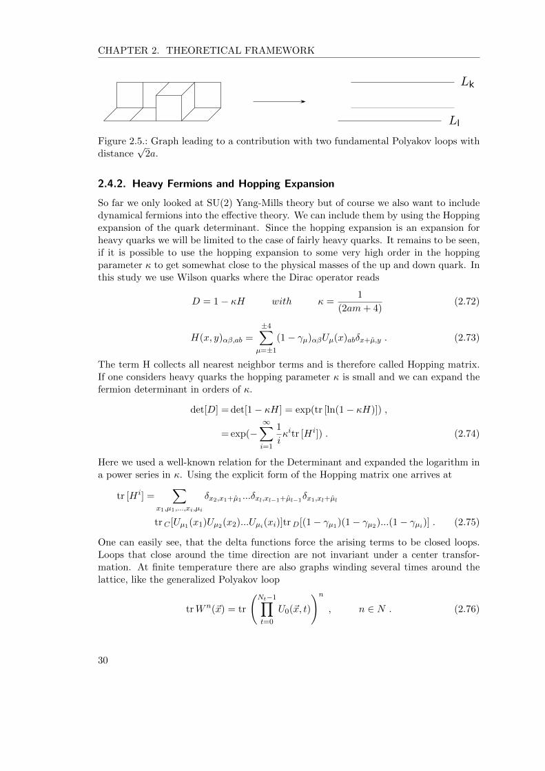
CHAPTER 2. THEORETICAL FRAMEWORK
Lk
Ll
Figure 2.5.: Graph leading to a contribution with two fundamental Polyakov loops withdistance
√2a.
2.4.2. Heavy Fermions and Hopping Expansion
So far we only looked at SU(2) Yang-Mills theory but of course we also want to includedynamical fermions into the effective theory. We can include them by using the Hoppingexpansion of the quark determinant. Since the hopping expansion is an expansion forheavy quarks we will be limited to the case of fairly heavy quarks. It remains to be seen,if it is possible to use the hopping expansion to some very high order in the hoppingparameter κ to get somewhat close to the physical masses of the up and down quark. Inthis study we use Wilson quarks where the Dirac operator reads
D = 1− κH with κ =1
(2am+ 4)(2.72)
H(x, y)αβ,ab =±4∑
µ=±1
(1− γµ)αβUµ(x)abδx+µ,y . (2.73)
The term H collects all nearest neighbor terms and is therefore called Hopping matrix.If one considers heavy quarks the hopping parameter κ is small and we can expand thefermion determinant in orders of κ.
det[D] = det[1− κH] = exp(tr [ln(1− κH)]) ,
= exp(−∞∑i=1
1
iκitr [H i]) . (2.74)
Here we used a well-known relation for the Determinant and expanded the logarithm ina power series in κ. Using the explicit form of the Hopping matrix one arrives at
tr [H i] =∑
x1,µ1,...,xi,µi
δx2,x1+µ1 ...δxl,xl−1+µl−1δx1,xl+µl
tr C [Uµ1(x1)Uµ2(x2)...Uµi(xi)]trD[(1− γµ1)(1− γµ2)...(1− γµi)] . (2.75)
One can easily see, that the delta functions force the arising terms to be closed loops.Loops that close around the time direction are not invariant under a center transfor-mation. At finite temperature there are also graphs winding several times around thelattice, like the generalized Polyakov loop
trWn(~x) = tr
(Nt−1∏t=0
U0(~x, t)
)n, n ∈ N . (2.76)
30

2.4. Effective Polyakov-Loop Theories
We obtain the effective action from the full partition function in a way similar to puregauge theory. First, use the hopping expansion to get a representation of fermion deter-minant as in (2.74). If one has the determinant in this form one can again use a clusterexpansion
Z =
∫[dU0][dUi] exp[−Sg] det[D] =
∫[dU0] exp[−Seff] ,
−Seff = ln
∫[dUi] exp[−Sg] det[D] . (2.77)
Again similar to the cluster expansion of the pure gauge theory only graphs windingaround the temporal direction of the lattice contribute to the effective action. There-fore the leading order contributions from the fermion determinant are terms containingPolyakov loops
−∑~x
[(2κeaµ)NtL(~x) + (2κe−aµ)NtL(~x)
], (2.78)
with
h = (2κeaµ)Nt , h = (2κe−aµ)Nt . (2.79)
The first term is a contribution from loops winding around the lattice in positive timedirection while the second term comes from loops oriented in negative temporal direction.For SU(2) the only difference in those terms are the effective couplings h and h whichdiffer in the case of non-vanishing chemical potential µ. The overall minus sign is dueto the anti-periodic boundary conditions for fermions. It now is possible to sum upall generalized Polyakov loops oriented in the same direction, particularly for positivetemporal direction
exp
[−2∑~x
∞∑n=1
((−1)n
nh tr (Wn
~x )
)]=∏~x
det [1 + hW~x]2 . (2.80)
The partition function for the effective theory to leading order in strong coupling andhopping expansion reads
Z =
∫[dU0]
∏<~x~y>
[1 + λ1L~xL~y
]∏~x
det[(1 + hW~x)(1 + hW †~x)
]2. (2.81)
We can simplify the result even more by using a simple rule for the determinant in SU(2)
det[1 + CW ] = 1 + Ctr [W ] + C2 . (2.82)
By changing the integration measure
∫ [Nt−1∏t=1
dU0(~x, t)
]=
∫dW~x =
∫ +2
−2dL~x e
V~x , V~x =1
2ln(4− L2
~x) ,
31

CHAPTER 2. THEORETICAL FRAMEWORK
our result for the partition function reads
Z =
∫ (∏~x
dL~x eV~xX~x(h, h)
) ∏<~x~y>
[1 + λ1L~xL~y
], (2.83)
and
X~x(h, h) = [(1 + hL~x + h2)(1 + hL~x + h2)]2 . (2.84)
With this result we have a dimensionally reduced effective theory that includes dynamicalfermions with only SU(2) Polyakov loops as degrees of freedom.
2.4.3. Corrections to the Effective Fermion Coupling
Like in the case of pure gauge theory there are corrections to the effective fermioncouplings. Those corrections will be the same for h and h since the two only differby the sign of the chemical potential. Corrections to leading order in κ are comingfrom graphs that also contain spatial link variables that are integrated out. The firstcorrection is the plaquette term with O(κ4). Since this graph does not wind around thelattice it will not yield a correction of h but a correction in the gauge term leading to ashift in β an thus a κ dependence of u
β → β + 48κ4 ⇒ u(β)→ u(β, κ) . (2.85)
Let us now consider corrections to the effective fermion couplings. Figure 2.6 showsgraphs leading to O(κ2ul) corrections after spatial integration. Here we have to includeadditional plaquettes from the strong coupling expansion of the gauge action, otherwisethe integration over the spatial links would vanish. One can sum up all correctionscoming from decorations with 1 ≤ l ≤ Nt − 1 additional plaquettes
(2κeaµ)Nt6Ntκ2Nt−1∑l=1
ul = (2κeaµ)Nt6Ntκ2u− uNt
1− u. (2.86)
Again, successive decorations lead to exponentiation. Therefore, including all correctionsup to O(unκm), with n+m = 7, we obtain
h(u, κ,Nt ≥ 4) = (2κeaµ)Nt exp
[6Ntκ
2u
(1− uNt−1
1− u
+4u4 − 8κ2 + 9κ2u+ 4κ2u2)]
. (2.87)
It is possible to show, that for free quarks in leading order hopping expansion the quarkmass, extracted from the pole of the propagator is am = − log(2κ). Therefore we caninterpret h as
h = exp
(µ−mT
), (2.88)
32

2.4. Effective Polyakov-Loop Theories
Figure 2.6.: Graphs reducing to Polyakov loops after spatial link integration resulting inO(κ2ul)corrections, with 1 ≤ l ≤ Nt − 1
and the corrections from decorations correspond to corrections to the quark mass
am = − log(2κ)− 6Ntκ2u
(1− uNt−1
1− u+ 4u4 − 8κ2 + 9κ2u+ 4κ2u2
). (2.89)
This form of the effective fermion coupling has an important consequence on the validityof the effective theory. In eq. (2.80) we have resummed all multiple winding loops toa log. The radius of convergence for this series is |r| < 1. As the operator norm of thePolyakov line is ||W || = 1, the effective theory is only valid for h < 1, or respectivelyµ < mq. Let us state that the hopping expansion is convergent for any µ, it is justthe resummation of the multiple winding loops that diverges for µ ≥ mq. Howeverwe can still use the resummed effective theory for µ > mq in the sense of an analyticcontinuation and we will see that we get resonable results.
2.4.4. Fermions beyond Leading Order
So far, we only considered the so-called static quark determinant with corrections to theeffective fermion coupling. To go beyond this approximation, we will define the kineticquark determinant
det[D] = det[1− T+ − T− − S+ − S−] ,
= det[1− T+ − T−] det[1− (1− T )−1(S+ + S−)]
= det[Dstat] det[Dkin] , (2.90)
here, T± and S± denote hops in ± temporal or spatial directions. We already com-puted det[Dstat] in our LO analysis. We further split the kinetic determinant into partsdescribing quarks moving in positive and negative spatial directions, P =
∑k Pk and
M =∑
kMk. Since the trace in (2.90) is also a trace in coordinate space only closedloops contribute and we need the same number of P s and Ms.
det[Dkin] = det[1− (1− T )−1(S+ + S−)] ,
= det[1− P −M ] ,
= exp[tr log(1− P −M)] (2.91)
To order O(κ4) we have
det[Dkin] = exp
[−trPM − trPPMM − 1
2trPMPM
][1 +O(κ6)] , (2.92)
=
[1− trPM − trPPMM − 1
2trPMPM +
1
2(trPM)2
][1 +O(κ6)] .
33
CHAPTER 2. THEORETICAL FRAMEWORK
Now we need to make the directions of the hops visible. Again, P’s and M’s need tocome in pairs for every direction
∑ij
trPiMj =∑i
trPiMi , (2.93)
∑ijkl
trPiPjMkMl =∑i
trPiPiMiMi +∑i 6=j
trPiPjMiMj +∑i 6=j
trPiPjMjMi ,
(2.94)
1
2
∑ijkl
trPiMjPkMl =1
2
∑i
trPiMiPiMi +1
2
∑i 6=j
trPiMiPjMj +1
2
∑i 6=j
trPiMjPiMj ,
(2.95)
1
2
∑ijkl
trPiMjtrPkMl =1
2
∑i,j
trPiMitrPjMj . (2.96)
Now let us shed some more light on the static quark propagator (1− T )−1 that appearsin equation (2.91). From (1 + γµ)(1 − γµ) = 0 we can immediately see, that hops inpositive and negative time-direction do not mix and we therefore get
(Dstat)−1 = (D+
stat)−1 + (D−stat)
−1 − 1 . (2.97)
We can now use a series expansion for the hops in positive time-direction
(D+stat)
−1 = (1− T+)−1 =∞∑n=0
(T+)n . (2.98)
We then find
(D+stat)
−1t1,t2
= δt1,t2(1− qzNtW ) + qzt2−t1W (t2, t1)[θ(t2 − t1)− zNtθ(t1 − t2)
], (2.99)
q =1
2(1 + γ0)(1 + zNtW )−1 , z = 2κeaµ . (2.100)
W (t2, t1) is a temporal Wilson line and for t1 = t2 we have a Polyakov lineW (t1, t1) = W .The contribution to the propagator in negative time direction is obtained analogously:
(D−stat)−1t1,t2
= δt1,t2(1− qzNtW †) + qzt1−t2W †(t1, t2)[θ(t1 − t2)− zNtθ(t2 − t1)
],
(2.101)
q =1
2(1 + γ0)(1 + zNtW †)−1 , z = 2κe−aµ . (2.102)
34
2.4. Effective Polyakov-Loop Theories
It will be convenient, to split the propagator in propagation direction as well as in Diracspace:
(Dstat)−1 = A+ γ0B = A+γ0B
+ +A− − γ0B− , (2.103)
A+xy =
1
2
[1− hW
1 + hW
]δxy +
1
2zty−tx
W (tx, ty)
1 + hW[θ(ty − tx)− hθ(tx − ty)] δ~x~y ,
B+xy = −1
2
hW
1 + hWδxy +
1
2zty−tx
W (tx, ty)
1 + hW[θ(ty − tx)− hθ(tx − ty)] δ~x~y ,
A−xy =1
2
[1− hW †
1 + hW †
]δxy +
1
2ztx−ty
W †(tx, ty)
1 + hW †[θ(tx − ty)− hθ(tx − ty)
]δ~x~y ,
B−xy = −1
2
hW †
1 + hW †+
1
2ztx−ty
W †(tx, ty)
1 + hW †[θ(tx − ty)− hθ(ty − tx)
]δ~x~y .
Note, that the coordinates without vector arrows are space-time coordinates, and thatwe already included corrections from spatial hops by replacing zNt with h from (2.87).It is very important to realize that this form of the static propagator is also valid forh < 1, due to the convergence criterion for the geometric series. We will now collect allthe terms, take the trace in Dirac and position space and perform the group integration.
Taking Traces
When we deal with more than one combination of trPiMi, it will also be necessary to ex-plicitly display the spatial coordinates. We will distinguish between terms, coupling two,three or even four spatial coordinates and we will call those term n-point interactions.
Two-Point Interactions
Up to order κ4 we find three terms involving two-point interactions
e−Sf =
∫[dUk]
−∑i
trPiMi −1
2
∑i
trPiMiPiMi +1
2
∑~x,i
trP~x,iM~x,itrP~x,iM~x,i
.
The first contribution is of order κ2:
−∫
[dUk]∑i
trPiMi = −∑i
∫[dUk]tr
[D−1
statS+i D
−1statS
−i
], (2.104)
= −8κ2
Nc
∑u,i
trBu,utrBu+i,u+i ,
= −2κ2Nt
Nc
∑~x,i
[(tr
hW~x
1 + hW~x− tr
hW †~x
1 + hW †~x
)(tr
hW~x+i
1 + hW~x+i− tr
hW †~x+i
1 + hW †~x+i
)].
Group integration was performed using eq. (2.63). This forces the link variables to beat the same position. Therefore the two temporal traces only result in a factor of Nt not
35
CHAPTER 2. THEORETICAL FRAMEWORK
N2t . The next contribution to the two-point interaction is of the order κ4. For this term
we will show the derivation of the final result in great detail. The reader should then inprinciple be able to reproduce the calculations for all other terms:
− 1
2
∫[dUk]
∑i
trPiMiPiMi = , (2.105)
− 1
2
∑i
∫[dUk]tr [D−1
statS+D−1
statS−D−1
statS+D−1
statS−] ,
= −1
2
∑i
∫[dUk]tr
[(A+ γ0B)κ(1 + γi)Ui(A+ γ0B)κ(1− γi)U †i
(A+ γ0B)κ(1 + γi)Ui(A+ γ0B)κ(1− γi)U †i].
Now we take a closer look on the trace in Dirac space:
trD [(A+ γ0B)(1 + γi)(A+ γ0B)(1− γi)(A+ γ0B)(1 + γi)(A+ γ0B)(1− γi)] .
It is easy to see that all terms containing an A will vanish, since for those terms wealways have an (1 + γi)(1− γi) = 0. We then find
trD [γ0B(1 + γi)γ0B(1− γi)γ0B(1 + γi)γ0B(1− γi)] = , (2.106)
trD [B(1− γi)B(1− γi)B(1− γi)B(1− γi)] ,= trD[B4(1− γi)4] = 32B4 .
When we plug this result back into eq. (2.105) we arrive at
− 1
2
∫[dUk]
∑i
trPiMiPiMi = , (2.107)
− 16κ4∑~x,i,t[ξ]
∫[dUk]Bab(~x, tα, tβ)Ubc(~x, tβ, i)Bcd(~x+ i, tβ, tγ)U †de(~x+ i, tγ , i)
Bef (~x, tγ , tδ)Ufg(~x, tδ, i)Bgh(~x+ i, tδ, tα)U †ha(~x+ i, tα, i) .
Here we made all indices and coordinates explicit, latin indices denote color indices.Because of the overall trace we have to have a closed loop in space-time and we have tohave a trace in color-space. Now we have to perform the group integral. There are onlythree combinations of the U ’s and U †’s where the group integral does not vanish:
• There are one U and one U † per link: use eq. (2.63) as integration rule
• All U and U † occupy the same link [87]:∫dUUi1j1Ui2j2U
†k1l1
U †k2l2=
1
N2c − 1
(δi1l1δi2l2δj1k1δj2k2 + δi1l2δi2l1δj1k2δj2k1)
(2.108)
− 1
Nc(N2c − 1)
(δi1l2δi2l1δj1k1δj2k2 + δi1l1δi2l2δj1k2δj2k1) ,
36
2.4. Effective Polyakov-Loop Theories
We will also end up with Kronecker deltas for the time coordinates, since pairs of timecoordinates or even all coordinates have to be the same. Then we arrive at
− 1
2
∫[dUk]
∑i
trPiMiPiMi = (2.109)
− 16κ4
N2c
∑~x,t1 6=t2,i
[trB(~x, t1, t2)B(~x, t2, t1)(trB(~x+ i, t1, t1))2
+ (trB(~x, t1, t1))2trB(~x+ i, t1, t2)B(~x+ i, t2, t1)]
− 16κ4
N2c − 1
∑~x,t,i
trB(~x, t, t)B(~x, t, t)(trB(~x+ i, t, t))2 + (trB(~x, t, t))2trB(~x+ i, t, t)B(~x+ i, t, t)
− 1
Nc[trB(~x, t, t)B(~x, t, t)trB(~x+ i, t, t)B(~x+ i, t, t) + (trB(~x, t, t))2(trB(~x+ i, t, t))2] ,
or in a more compact form with the 4-vectors u, v:
− 1
2
∫[dUk]
∑i
trPiMiPiMi = (2.110)
− 16κ4
N2c
∑u6=v,i
[trBu,vBv,u(trBu+i,u+i)
2 + (trBu,u)2trBu+i,v+iBv+i,u+i
]− 16κ4
N2c − 1
∑u,i
trBu,uBu,u(trBu+i,u+i)2 + (trBu,u)2trBu+i,u+iBu+i,u+i
− 1
Nc[trBu,uBu,utrBu+i,u+iBu+i,u+i + (trBu,u)2(trBu+i,u+i)
2] .
37
CHAPTER 2. THEORETICAL FRAMEWORK
When we now use the definition for B from eq. (2.103) and perform the sum over thetime indices we arrive at
−1
2
∫[dUk]
∑~x,i
TrP~x,iM~x,iP~x,iM~x,i = (2.111)
κ4Nt(Nt − 1)
N2c
∑~x,i
Tr( hW~x
(1 + hW~x)2+
hW †~x
(1 + hW †~x)2+ 2
1Nt−1
∑Nt−1t=1 (2κ)2t
(1 + hW~x)(1 + hW †~x)
)(
TrhW~x+i
1 + hW~x+i− Tr
hW †~x+i
1 + hW †~x+i
)2+(
TrhW~x
1 + hW~x− Tr
hW †~x
1 + hW †~x
)2
Tr( hW~x+i
(1 + hW~x+i)2+
hW †~x+i
(1 + hW †~x+i)2
+ 21
Nt−1
∑Nt−1t=1 (2κ)2t
(1 + hW~x+i)(1 + hW †~x+i)
)− κ4Nt
N2c − 1
∑~x,i
Tr( hW~x
1 + hW~x−
hW †~x
1 + hW †~x
)2(Tr
hW~x+i
1 + hW~x+i− Tr
hW †~x+i
1 + hW †~x+i
)2
+(
TrhW~x
1 + hW~x− Tr
hW †~x
1 + hW †~x
)2Tr( hW~x+i
1 + hW~x+i−
hW †~x+i
1 + hW †~x+i
)2+
κ4Nt
N3c −Nc
∑~x,i
Tr( hW~x
1 + hW~x−
hW †~x
1 + hW †~x
)2Tr( hW~x+i
1 + hW~x+i−
hW †~x+i
1 + hW †~x+i
)2
+(
TrhW~x
1 + hW~x− Tr
hW †~x
1 + hW †~x
)2(Tr
hW~x+i
1 + hW~x+i− Tr
hW †~x+i
1 + hW †~x+i
)2.
Again we have replaced all factors zNt with h, to include corrections from spatial hops,and since we want to apply our model in the cold and dense regime, we drop all termsthat are subleading in Nt and have h ∼ e−aµNt → 0 . In this limit the expression abovereduces to
− 1
2
∫[dUk]
∑i
trPiMiPiMi =
κ4N2t
N2c
∑~x,i
trhW~x
(1 + hW~x)2
[(tr
hW~x+i
1 + hW~x+i
)2+(
trhW~x−i
1 + hW~x−i
)2], (2.112)
38

2.4. Effective Polyakov-Loop Theories
where we have relabeled the summation indices of the second term. Also, the nextcontribution to the two-point interactions is of order κ4:
1
2
∫[dUk]
∑~x,i
tr P~x,iM~x,itr P~x,iM~x,i (2.113)
=32κ4
N2c
∑u6=v,i
[(tr Bu,u
)2(tr Bv+ı,v+ı
)2+ tr Bu,vBv,utr Bu+ı,v+ıBv+ı,u+ı
]
+32κ4
N2c − 1
∑u,i
(tr Bu,u
)2(tr Bu+ı,u+ı
)2+ tr Bu,uBu,utr Bu+ı,u+ıBu+ı,u+ı
− 1
Nc
[tr Bu,uBu,u
(tr Bu+ı,u+ı
)2+(
tr Bu,u
)2tr Bu+ı,u+ıBu+ı,u+ı
].
These are all two-point interactions that one finds in general, other corrections to thetwo-point interaction start with O(κ6). However, for the special case of SU(2), there areadditional two-point interactions coming from dynamic diquark contributions. In theterms:
−1
2
∫dU∑i
trPiMiPiMi ,
1
2
∫dU∑i
trPiMitrPiMi ,
we find further non-vanishing combinations of the U ’s and U †’ from the group integrationrule for SU(2) ∫
dUUijUkl =1
2εikεjl . (2.114)
With this rule we can calculate the contributions from the dynamic diquarks to be
−1
2
∫dU∑i
trPiMiPiMi = −8κ4∑u6=v
det[Bu,v] det[Bv+i,u+i] ,
1
2
∫dU∑i
trPiMitrPiMi = 16κ4∑u6=v
det[Bu,v] det[Bv+i,u+i] ,
leading to an overall diquark contribution of
−Sdiquark = 8κ4∑u6=v
det[Bu,v] det[Bv+i,u+i] ,
= 2κ4N2t
∑x,i
deth
(1 + hWx)(1 + hWx+i)
= 2κ4N2t
∑x,i
h2
(1 + hLx + h2)(1 + hLx+i + h2)(2.115)
39
CHAPTER 2. THEORETICAL FRAMEWORK
Three-Point Interactions
Interactions connecting three spatial indices start at O(κ4)
e−Sf3 ≡
∫[dUk]
[−∑i
tr PiPiMiMi −∑i 6=j
tr PiPjMjMi (2.116)
−1
2
∑i 6=j
tr PiMiPjMj −1
2
∑i 6=j
tr PiMjPjMi +1
2
∑~x,~y,i,j
tr P~x,iM~x,itr P~y,jM~y,j
].
The different contributions are evaluated to be
−∫
[dUk]∑i
tr PiPiMiMi =
−32κ4
N2c
∑u,v,i
tr Bu,utr Au+ı,v+ıAv+ı,u+ıtr Bu+2ı,u+2ı , (2.117)
−∫
[dUk]∑i 6=j
tr PiPjMjMi =
−16κ4
N2c
∑u,v,i6=j
tr Bu−ı,u−ı
[tr Au,vAv,u + tr Bu,vBv,u
]tr Bu+,u+ , (2.118)
−1
2
∫[dUk]
∑i 6=j
tr PiMiPjMj =
−8κ4
N2c
∑u,v,i6=j
tr Bu+ı,u+ı
[tr Au,vAv,u + tr Bu,vBv,u
]tr Bu+,u+ ,
(2.119)
−1
2
∫[dUk]
∑i 6=j
tr PiMjPjMi =
−8κ4
N2c
∑u,v,i6=j
tr Bu−ı,u−ı
[tr Au,vAv,u + tr Bu,vBv,u
]tr Bu−,u− ,
(2.120)
1
2
∫[dUk]
∑~x,~y,i,j
tr P~x,iM~x,itr P~y,jM~y,j =
32κ4
N2c
∑u,v,i,j
tr Bu,utr Bu+ı,u+ıtr Bv,vtr Bv+,v+ , (2.121)
where the sum is only over terms where the two traces share one spatial point.
40

2.4. Effective Polyakov-Loop Theories
Four-point Interactions
There are only two four-point interactions to order κ4
e−Sf4 ≡
∫[dUk]
[−∑i 6=j
tr PiPjMiMj +1
2
∑~x,~y,i,j
tr P~x,iM~x,itr P~y,jM~y,j
]. (2.122)
After integration the first contribution vanishes in the strong coupling limit and onlygives a non-zero contribution if a plaquette is inserted into the fermionic loop:∫
[dUk]∑i 6=j
tr PiPjMiMj = O(κ4u) . (2.123)
Since we only calculate the action to order κmun with m+ n = 4 we neglect this term.The second contribution is
1
2
∫[dUk]
∑~x,~y,i,j
tr P~x,iM~x,itr P~y,jM~y,j = (2.124)
32κ4
N2c
∑u,v,i,j
tr Bu,utr Bu+ı,u+ıtr Bv,vtr Bv+,v+ ,
where the sum is only over terms where the traces share no common spatial point.
2.4.5. Resummation
Remember that we had to expand the exponential in the kinetic part of the fermiondeterminant to be able to perform the group integrations
det[Dkin] = exp[− trPM − trPPMM − 1
2trPMPM
], (2.125)
= 1− trPM − trPPMM − 1
2trPMPM +
1
2(trPM)2 +O(κ6) .
Now, we have all those terms after integration. Our goal is now to resum the resultingterms back into an exponential to improve convergence and take as many terms of theoriginal exponential into account as we can. The resummation for the κ2 term looks like∫
[dUk]e−
∑i trPiMi = 1 − 8κ2
Nc
∑u,i
tr Bu,utr Bu+ı,u+ı
+32κ4
N2c
∑u,v,i,j
tr Bu,utr Bu+ı,u+ıtr Bv,vtr Bv+,v+
= e−8κ2
Nc
∑u,i tr Bu,utr Bu+ı,u+ı +O(κ6) . (2.126)
The form of the higher order terms indicates, that this procedure should always be valid.However the higher orders in eq. (2.126) have to be excluded from the appropriate ordersin κ to avoid over counting.
41

CHAPTER 2. THEORETICAL FRAMEWORK
2.4.6. Effective Action for the Cold and Dense Regime
We now have all the ingredients to write down the effective action for the cold and denseregime. We have to add up and resum all the terms we have evaluated in the last section.One has to be a little careful as there are some terms that can lead to double countingin the resummation, however in general this procedure is straightforward. As alreadymentioned above, we will neglect all terms proportional to h and all terms subleadingin Nt, which is reasonable for µ > 0 and T → 0. Further, we find that the effectivegauge coupling λ becomes negligible λ(β = 2.5, Nt = 200) ∼ 1 ·10−15. Therefore, we willcompletely drop the effective gauge action of our theory. Yet, there are still remnantsof the Yang-Mills part in our effective theory. As mentioned in section 2.4.3, there aregauge corrections to the effective fermion coupling h, see eq. (2.87). The effective actionfor the cold and dense regime for one flavor reads
− Seff =∑~x
log(1 + hLi + h2)2 − 2h2
∑~x,i
trhW~x
1 + hW~xtr
hW~x+i
1 + hW~x+i
+ 2κ4N2
t
N2c
∑~x,i
trhW~x
(1 + hW~x)2tr
hW~x+i
(1 + hW~x+i)2
+κ4N2
t
N2c
∑~x,i,j
trhW~x
(1 + hW~x)2tr
hW~x−i1 + hW~x−i
trhW~x−j
1 + hW~x−j
+ 2κ4N2
t
N2c
∑~x,i,j
trhW~x
(1 + hW~x)2tr
hW~x−i1 + hW~x−i
trhW~x+j
1 + hW~x+j
+κ4N2
t
N2c
∑~x,i,j
trhW~x
(1 + hW~x)2tr
hW~x+i
1 + hW~x+itr
hW~x+j
1 + hW~x+j
− 2κ4N2t
∑x,i
h
(1 + hLx + h2)(1 + hLx+i + h2). (2.127)
We have introduced a new coupling h2, which also results from gauge corrections to theO(κ2) coupling
h2 =κ2Nt
Nc
[1 + 2
u− uNt1− u
+ . . .
]. (2.128)
The gauge corrections to this coupling do not seem to exponentiate [84]. One shouldalso remember, that the last term of eq. (2.127) is only there in two- color QCD. Ingeneral SU(N) gauge theories similar terms will start to emerge in order κ2N .
2.4.7. Effective Action for Nf Flavors
We will now discuss how to extend the effective model to more than one quark flavor.When we take all flavors to be degenerate, the partition function is modified to
Z =
∫dUe−Sg det[D]Nf , (2.129)
42
2.4. Effective Polyakov-Loop Theories
where we just get additional fermion determinants from each flavor. Again, we can splitup the fermion determinants in terms of static and kinetic parts and expand the kineticpart in powers of the hopping parameter. We now find
det[D]Nf = (det[Dstat] det[Dkin])Nf ,
= det[Dstat]Nf exp
[−Nf trPM −Nf trPPMM
−Nf
2trPMPM
][1 +O(k6)] ,
= det[Dstat]Nf
[1−Nf trPM −Nf trPPMM −
Nf
2trPMPM
+Nf
2
2(trPM)2
][1 +O(k6)] .
When we compare this result with the one from eq. (2.92) we can conclude that theeffective action for the Nf -flavor case will consist of the same terms as for Nf = 1 withdifferent prefactors. The effective action for Nf flavors of degenerate quarks reads
− Seff = Nf
∑~x
log(1 + hLi + h2)2 − 2Nfh2
∑~x,i
trhW~x
1 + hW~xtr
hW~x+i
1 + hW~x+i
+ 2N2f
κ4N2t
N2c
∑~x,i
trhW~x
(1 + hW~x)2tr
hW~x+i
(1 + hW~x+i)2
+Nfκ4N2
t
N2c
∑~x,i,j
trhW~x
(1 + hW~x)2tr
hW~x−i1 + hW~x−i
trhW~x−j
1 + hW~x−j
+ 2Nfκ4N2
t
N2c
∑~x,i,j
trhW~x
(1 + hW~x)2tr
hW~x−i1 + hW~x−i
trhW~x+j
1 + hW~x+j
+Nfκ4N2
t
N2c
∑~x,i,j
trhW~x
(1 + hW~x)2tr
hW~x+i
1 + hW~x+itr
hW~x+j
1 + hW~x+j
− 2(2N2f −Nf )κ4N2
t
∑x,i
h2
(1 + hLx + h2)(1 + hLx+i + h2). (2.130)
2.4.8. Mass Scale
In order to establish a reference scale for our simulations at finite density, we calculatethe diquark or respectively the pion mass in the vacuum in the hopping expansion. Weextract the mass from the exponential decay of the following pion correlator
am(π) = limt→∞
1
tln〈π(0)π(t)〉 , (2.131)
where we have to sum over space-like indices in order to have mass eigenstates [88]
π(t) =∑~x
π(~x, t) . (2.132)
43

CHAPTER 2. THEORETICAL FRAMEWORK
The pion correlator is of the form
〈π(0)π(t)〉 = 〈d(0)γ5u(0)u(t)γ5d(t)〉 . (2.133)
Applying the Wick theorem and keeping in mind that one can only contract fermionfields with equal flavor (also in the case of degenerate quark masses), we arrive at
〈π(0)π(t)〉 = −〈tr [γ5D−1(0, t)γ5D
−1(t, 0)]〉QCD (2.134)
Now, hopping expand the pion propagator up to order O(κ2). The index QCD of theexpectation value means, that up to now we cannot integrate out the spatial links buthave to use the full theory. Only after expanding the quark propagator we can integrateover the spatial links. Remember, nly diagrams that give non-vanishing contributionsto the link integration will show up in the pion propagator.To LO, these are just two anti-parallel temporal gauge-link chains running between 0and t. The computation of their contribution is analogous to the LO hopping expansionof the fermion determinant
〈π(0)π(t)〉LO ∝ (2κ)(2t) (2.135)
To order O(κ2) we have five different contributions, one without and four with attachedgauge plaquettes. Figure 2.7 shows all diagrams to order O(κ2). The O(κ2) decorationsare (in the limit of large t)
6tκ2 + 24tκ2u− ut+1
1− u. (2.136)
In the order O(κ4u0) we have only anti-parallel gauge-link chains, each with two hops inspatial direction. We get 6t · 6(t−1) diagrams with hops at different temporal coordinatesand 6 · 5t diagrams with two hops at the same temporal coordinate. Again, we wouldcount the terms proportional to t2 twice when exponentiating repeating contributions,leading to the O(κ4u0) contribution
(−36t+ 30t)κ4 = −6tκ4 , (2.137)
As in the hopping expansion of the fermion determinant, repeating corrections lead toexponentiation and the pion propagator becomes
〈π(0)π(t)〉NLO ∝ (2κ)(2t) exp
[6tκ2 + 24tκ2u− ut+1
1− u− 6tκ4
]. (2.138)
By plugging this result into (2.131) we get the mass of the pion
am(π) = −2 ln(2κ)− 6κ2 − 24κ2 u
1− u+ 6κ4 +O(κ4u2, κ2u5) . (2.139)
We can even improve this result by using the pion mass for a free theory from [89],which includes the meson propagator to all orders in κ, together with our string couplingcorrections. There are still corrections from the hopping expansion of the effective action,but they will only start to give contributions at O(κ6). The pion mass is then given by
am(π) = arcosh
(1 +
(1− 16κ2)(1− 4κ2)
8κ2(1− 6κ2)
)− 24κ2 u
1− u+O(κ4u2, κ2u5, κ6) . (2.140)
44
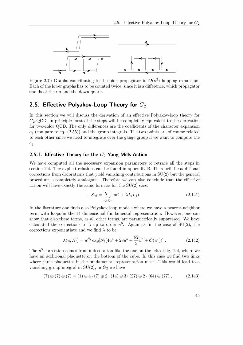
2.5. Effective Polyakov-Loop Theory for G2
Figure 2.7.: Graphs contributing to the pion propagator in O(κ2) hopping expansion.Each of the lower graphs has to be counted twice, since it is a difference, which propagatorstands of the up and the down quark.
2.5. Effective Polyakov-Loop Theory for G2
In this section we will discuss the derivation of an effective Polyakov-loop theory forG2-QCD. In principle most of the steps will be completely equivalent to the derivationfor two-color QCD. The only differences are the coefficients of the character expansionaj (compare to eq. (2.55)) and the group integrals. The two points are of course relatedto each other since we need to integrate over the gauge group if we want to compute theaj .
2.5.1. Effective Theory for the G2 Yang-Mills Action
We have computed all the necessary expansion parameters to retrace all the steps insection 2.4. The explicit relations can be found in appendix B. There will be additionalcorrections from decorations that yield vanishing contributions in SU(2) but the generalprocedure is completely analogous. Therefore we can also conclude that the effectiveaction will have exactly the same form as for the SU(2) case:
−Seff =∑<ij>
ln(1 + λLiLj) . (2.141)
In the literature one finds also Polyakov loop models where we have a nearest-neighborterm with loops in the 14 dimensional fundamental representation. However, one canshow that also these terms, as all other terms, are parametrically suppressed. We havecalculated the corrections to λ up to order u6. Again as, in the case of SU(2), thecorrections exponentiate and we find λ to be
λ(u,Nt) = uNt exp[Nt(4u4 + 28u5 +
82
3u6 +O(u7))] . (2.142)
The u5 correction comes from a decoration like the one on the left of fig. 2.4, where wehave an additional plaquette on the bottom of the cube. In this case we find two linkswhere three plaquettes in the fundamental representation meet. This would lead to avanishing group integral in SU(2), in G2 we have
(7)⊗ (7)⊗ (7) = (1)⊕ 4 · (7)⊕ 2 · (14)⊕ 3 · (27)⊕ 2 · (64)⊕ (77) , (2.143)
45
CHAPTER 2. THEORETICAL FRAMEWORK
and the trivial representation in the Clebsch-Gordon series leads to a non-vanishinggroup integral of the form:∫
dU UabUcdUef =1
14cacecbdf ,
cace =1√3ψace , a, c, e ∈ 1, 2, . . . , 7 , (2.144)
where ψace is the totally antisymmetric octonionic tensor defined by [72]
ψ123 = ψ147 = ψ165 = ψ246 = ψ257 = ψ354 = ψ367 = 1 . (2.145)
Also, there is a similar, additional diagram contributing to order O(u6). Here, we havea plaquette in the adjoint representation at the bottom of the cube. The higher theorder in u, the harder it gets to calculate the contributions from decorations as there area lot of combinations of plaquettes in various representations that give non-vanishingcontributions.
2.5.2. Leading Order Heavy Fermions for G2
Our strategy to include dynamical fermions into the effective theory is described indetail in section 2.4.2. The general procedure stays the same. And we again arrive atthe partition function from eq. (2.81):
Z =
∫[dU0]
∏<ij>
[1 + λ1LiLj ]∏~x
det[(1 + hW~x)(1 + hW T
~x )]2,
=
∫[dU0]
∏<ij>
[1 + λ1LiLj ]∏~x
det[(1 + hW~x)(1 + hW~x)
]2.
For SU(2) we were able to simplify this expression by rewriting the determinant as acharacteristic polynomial and expand in invariants of tensors
pW (λ) =n∑k=0
(−1)kλn−ktr (ΛkW ) , (2.146)
where tr (ΛkW ) is the trace of the k-th exterior power, or respectively one of the ktensor invariants. The idea behind this expansion is to express the determinant in termsof traces, so we do not have to sample over the full gauge group in the Monte-Carlosimulation, but only over the class angles. SU(2) has rank 1 and there is exactly oneinvariant trW . For SU(3) with rank 2 we have one more invariant which can be chosento be trW †. Elements of G2 are represented by 7x7 matrices. For a 7x7 matrix wegenerally find seven tensor invariants, however because of the structure of G2 they arenot independent [72], but the relations are more involved than in the simple cases ofSU(2) or SU(3). We do not need this expression in our simulations as it will not lead toa algorithmic speed up but will use the eigenvalues of W . However, as for the case of
46
2.5. Effective Polyakov-Loop Theory for G2
SU(2), one can use this expression to get e.g. insight into the spectrum of the effectivetheory.Getting the G2 equivalent of eq. (2.82) is more challenging as it is for SU(2) oder SU(3).However, if we use the fact that the determinant is a class function, it is sufficient touse elements t from the maximal torus T of G2 (see appendix C). Examining t a littlecloser, we see that we can write
t =
u u∗
1
with u =
eiϕ eiϑ
e−i(ϕ+ϑ)
, (2.147)
where u is an element of the maximal torus of SU(3) and ϕ, ϑ ∈ [0, 2π]. So we can splitup the G2 determinant in two SU(3) determinants with an additional factor
det [1 + hWG2 ] =[det(1 + huSU(3)) det(1 + hu†SU(3))(1 + h)
]. (2.148)
Now we can use the SU(3) equivalent of (2.82)
det[1 + huSU(3)] = 1 + hL+ h2L∗ + h3 with L = truSU(3) , (2.149)
to rewrite the SU(3) determinants and arrive at
det [1 + hWG2 ] =[(1 + hL+ h2L∗ + h3)(1 + hL∗ + h2L+ h3)(1 + h)
]. (2.150)
We now have the LO fermion content in terms of SU(3) Polyakov loops. However, we stillhave to perform the G2 group integral. Although, one can measure the SU(3) Polyakovloop in a G2 lattice simulation, it is not exactly clear what its physical meaning is. Sowe would like to transform this awkward expression into one with G2 Polyakov loops,since we know that G2 has rank 2, we expect to need two different tensor invariants. Thefirst two candidates that come to mind are the Polyakov loops in the two fundamentalrepresentations χ7 and χ14. It is now straight forward to expand eq. (2.150), plug in theSU(3) Polyakov loops in terms of the class angles, look at χ7 and χ14, again in terms ofclass angles, and find the result by equating coefficients:
det [1 + hWG2 ] = 1 + (h+ h6)χ7 + (h2 + h5)(χ7 + χ14)
+ (h3 + h4)(χ27 − χ14) + h7 . (2.151)
Thus the LO fermion contribution is given by
det [1 + hWG2 ]2 = 1 + (h+ h13)(2χ7) + (h2 + h12)(2χ14 + 2χ27 + 2χ7)
+ (h3 + h11)(4χ27 + 2χ14χ7 − 2χ14) + (h4 + h10)(3χ3
7 + χ214 + 3χ2
7 − 2χ14)
+ (h5 + h9)(4χ37 + 2χ14χ
27 − 2χ2
14 − 4χ14χ7 + 2χ14 + 2χ7)
+ (h6 + h8)(χ47 + 2χ3
7 − χ214 + 2χ2
7 + 2χ7)]
+ h7(2 + 2χ47 − 4χ2
7χ14 + 4χ214 + 4χ14χ7) + h14 . (2.152)
47
CHAPTER 2. THEORETICAL FRAMEWORK
Also different is h, since the derivation of h also involves group integrals. The effectivefermion coupling for G2 is given by
h(u, κ,Nt) = (2κeaµ)Nt exp[6Ntκ
2u(1− uNt−1
1− u+ 4u4 − 28κ2 + 9κ2u+ 4κ2u2
)]. (2.153)
2.5.3. Kinetic Fermion Determinant for G2
We reevaluate all terms in section 2.4.4, this time with gauge group G2. The basic groupintegrals for G2 is the same as in SU(N). We can even recycle the integration rule for alink occupied by UU †UU † in eq. (2.108). There is one additional non-vanishing groupintegral. Since G2 is a real subgroup of SO(7) we can evaluate it with the help of thebasic integration rule ∫
dU UabUcd =
∫dU UabU
−1dc =
1
7δacδbd . (2.154)
This again leads to additional terms in the two-point interaction
−1
2
∫dU∑i
trPiMiPiMi ,
1
2
∫dU∑i
trPiMitrPiMi ,
similar to the dynamic diquark contributions in the effective theory for two-color QCD.However for G2 it can be easily shown that those additional terms only result in a termindependent of temporal gauge links, so we can omit it when calculating expectationvalues. The effective action for the cold and dense regime of one-flavor G2-QCD thenreads
− Seff =∑~x
log det(1 + hW~x)2 − 2h2
∑~x,i
trhW~x
1 + hW~xtr
hW~x+i
1 + hW~x+i
+ 2κ4N2
t
N2c
∑~x,i
trhW~x
(1 + hW~x)2tr
hW~x+i
(1 + hW~x+i)2
+κ4N2
t
N2c
∑~x,i,j
trhW~x
(1 + hW~x)2tr
hW~x−i1 + hW~x−i
trhW~x−j
1 + hW~x−j
+ 2κ4N2
t
N2c
∑~x,i,j
trhW~x
(1 + hW~x)2tr
hW~x−i1 + hW~x−i
trhW~x+j
1 + hW~x+j
+κ4N2
t
N2c
∑~x,i,j
trhW~x
(1 + hW~x)2tr
hW~x+i
1 + hW~x+itr
hW~x+j
1 + hW~x+j(2.155)
where h2 is defined as in eq. (2.128).
48
3Results at Finite Temperature
Before turning to results in the phase diagram at finite baryon density, let us start bygiving some results from the effective theory at finite temperature but vanishing baryondensity. This serves to be an introduction to the finite temperature effects in our effectivetheory and, since there are plenty of results for both effective theories and full theories atfinite temperature, to test whether our implementation of the effective theory is correct.
3.1. Effective Polyakov-Loop Theory for SU(2)
We start by discussing results for the effective theories at finite temperature for SU(2)Yang-Mills theory. Later we will also show results from the effective theory with dynam-ical quarks.There are many studies on the finite temperature properties of SU(2) Yang-Mills andtwo-color QCD on the lattice, e.g. [45, 65, 75, 90–92] in the literature. There is alsoextensive work on effective Polyakov-loop theories for finite temperature SU(2) Yang-Mills theory [42, 44, 74, 81, 83]. Determining the critical effective coupling λc, βc(λc, Nt)and the order of the phase transition and then comparing this to existing results is anexcellent way to test the code for our numerical simulations.
3.1.1. Critical Coupling and Order of the Transition for SU(2)
Already in the early 80s, it was conjectured that a d + 1 dimensional SU(2) Yang-Mills theory has the same universal behavior as the d dimensional Ising model [74] andtherefore has a 2nd order deconfinement phase transition. This was later confirmed bylattice simulations with high accuracy (e.g. [45, 75]). From all these studies we expectour effective theory for SU(2) Yang-Mills theory with the partition function in eq. (2.71)to have a 2nd order phase transition with the universal properties of the 3d Ising model.
49

CHAPTER 3. RESULTS AT FINITE TEMPERATURE
0
0.1
0.2
0.3
0.4
0.5
0.6
0.7
0.8
0.18 0.19 0.2 0.21 0.22 0.23
<|L
|>
λ
Figure 3.1.: Polyakov loop 〈|L|〉 as a func-tion of the effective coupling λ for Ns = 16.
-0.1
0
0.1
0.2
0.3
0.4
0.5
0.6
0.7
0.21 0.212 0.214 0.216 0.218 0.22
B
λ
Ns=16 Ns=32 Ns=48
Figure 3.2.: Binder cumulant B(|L|) as afunction of the effective coupling λ for var-ious lattices sizes.
Fig. 3.1 shows the Polyakov loop 〈|L|〉 as a function of the effective coupling. Theplot shows the typical signs for a system with a second order phase transition in thethermodynamic limit. To check whether this is really the case and to determine theuniversality class and the critical coupling λc of the system one has to perform a finitesize scaling analysis. We will do this by using the 4th order Binder cumulant
B(|L|) = 1− 〈|L|4〉3〈|L|2〉2
. (3.1)
The use of the Binder cumulant has the advantage that finite size effects are muchreduced compared to analyzing the peak location and height in the susceptibilities. TheBinder cumulant for our system has the following properties
• confined phase: B(|L|) = −13 +O( 1
V ) as V →∞
• deconfined phase: B(|L|) + 23 +O( 1
V ) as V →∞
• at λc: B(|L|) tends towards a universal value B∗
Fig. 3.2 shows the Binder cumulant for three different lattice sizes. The lines intersectat λ = 0.21417(3) and B = 0.471(5), which we will take as the values for the criticalcoupling and the universal value for the Binder cumulant9. Our value for λc is in verygood agreement with the critical coupling λc = 0.21423(70) found by Langelage et al.[42] and the universal values for the Binder cumulant of the 3d Ising model B∗ = 0.470(5)and B∗ = 0.46575(11) [75].Since we now have the critical effective coupling λc we can use eqs. (2.69) to calculate the
9This is a little sloppy, as the the value of the Binder cumulant in the vicinity of the critical couplingscales like B ∼ B∗ + aN−a1s . However, since the finite volume dependence of the crossing point isvery small this will be sufficient for our purposes.
50

3.1. Effective Polyakov-Loop Theory for SU(2)
0
0.1
0.2
0.3
0.4
0.5
0.6
0.7
0.8
0.9
-1 -0.5 0 0.5 1
P(L
)
L
λ=0.073λ=0.180λ=0.190
YM: βc
Figure 3.3.: Polyakov loop distributionsP (L) for a naive Polyakov loop model andseveral effective couplings λ compared tothe distribution from a 4d lattice simula-tion at the critical coupling βc at Nt = 4.
0
0.1
0.2
0.3
0.4
0.5
0.6
0.7
0.8
0.9
-1 -0.5 0 0.5 1
P(L
)
L
λ=0.073λ=0.180λ=0.213
YM: βc
Figure 3.4.: Polyakov loop distributionsP (L) for the resummed Polyakov loopmodel and several effective couplings λcompared to the distribution from a 4d lat-tice simulation at the critical coupling βc atNt = 4.
critical lattice coupling βc to a given Nt. For Nt = 4, λc = 0.21423(70) corresponds toβc = 2.3102(08). Compared to the critical βc = 2.2991(2) from a full 4d lattice analysis[75] we have an accuracy of better than 1 %. At Nt = 16, λc leads to a critical couplingβc = 2.5582(02) while the 4d analysis from [93] finds βc = 2.7310(20), corresponding toan accuracy of about 6 %.
3.1.2. Comparison of Different Action
The amazing agreement of the critical coupling βc from full 4d simulations and from theeffective theory comes as a result of the resummations of the Polyakov loops with higherwinding numbers together with the order O(u12) corrections to the effective coupling λ.Already the resummation of the multiple-winding loops leads to a dramatic improvementof the effective theory. A quantity that shows this improvement is the per-site Polyakovloop probability distribution P (L) defined by
〈L〉 =
∫dLLP (L) . (3.2)
The Polyakov loop distribution can be measured by histograming the local Polyakovloop variable on the spatial lattice and aggregating over the whole ensemble. Full 4dlattice simulations have shown that the Polyakov loop distribution is given by the gaugegroup’s Vandermonde potential and remains unchanged up to the critical coupling βc[92, 94]. In the case of SU(2) the distribution is given by
P (L) =1
2π
√4− L2 . (3.3)
51
CHAPTER 3. RESULTS AT FINITE TEMPERATURE
Only if the coupling is increased further, the distributions are skewed and get asymmetricresulting in a non-zero expectation value for the Polyakov loop 〈L〉. We can now comparePolyakov loop distributions from full 4d lattice calculations in the confined phase todistributions from effective Polyakov loop models, also in the confined phase. Fig. 3.3shows the comparison of a distribution from a naive Polyakov loop model with nearestneighbor interaction
Seff = −λ∑〈ij〉
LiLj , (3.4)
with a distribution from a 4d lattice simulation at the critical coupling βc at Nt = 4.Note, that due to the different form of the effective action, the critical coupling for thiskind of model is λc = 0.18 [81]. We see that the distributions match only for very smallvalues of the effective coupling λ. For values close to the critical coupling λc = 0.18 wefind that the distributions from the naive effective theory are massively distorted andfor values λ ≈ λc we see some kind of double peak structure emerging. The Polyakovloop distributions from our model with the resummed action
Seff = −∑〈ij〉
log(1 + λLiLj) , (3.5)
are shown in Fig. 3.4. The critical coupling in this case is λc = 0.21417(3) and thedistributions match the distribution given by the Vandermonde determinant for almostall subcritical λ. We only see some minor deformations of the distributions close to λc.To see the effect of the corrections coming from decorations to the effective coupling λwe can compare the critical 4d coupling βc to the critical lattice coupling calculated byinversion of the LO strong coupling result from eq. (2.62)
λc = u(βc)Nt . (3.6)
For Nt = 4 this leads to βc = 4.3225 which is almost twice the known value βc = 2.2991.This gets even worse for bigger Nt as more decorations fit onto the lattice. For Nt = 16the critical beta from inversion of eq. (3.6) would be βc = 16.0678 compared to βc =2.7310. However, by including corrections from decorations up to order O(u12) we areable to restrict the errors in βc to about 6%.
3.1.3. Including Dynamical Fermions
Dynamical fermions in the fundamental representation of the gauge group break centersymmetry explicitly. Therefore we expect the second order deconfinement phase tran-sition of the pure gauge theory to turn into an analytic crossover. Fig. 3.5 shows thePolyakov loop 〈|L|〉 as a function of the effective gauge coupling λ for Ns = 16, withdynamical quarks and effective fermion coupling h = 0.004. Since we only want to showthe effect of the explicit breaking of center symmetry we only included the static part ofthe fermion determinant. If we compare this to fig. 3.1 we see that the phase transitionturns into a broad crossover, as expected.
52

3.2. Effective Polyakov-Loop Theory for G2 QCD
0
0.1
0.2
0.3
0.4
0.5
0.6
0.7
0.8
0.18 0.19 0.2 0.21 0.22 0.23
<|L
|>
λ
Figure 3.5.: Polyakov loop 〈|L|〉 as a function of the effective gauge coupling λ for Ns =16, with dynamical quarks and effective fermion coupling h = 0.004.
3.2. Effective Polyakov-Loop Theory for G2 QCD
We now turn our attention to the effective theory for the gauge group G2. Again westart with analyzing the effective theory in the case of pure gauge theory. Studies of G2
Yang-Mills and effective Polyakov-loop theories have found a 1st order deconfinementphase transition [50, 95]. First, we have to check if our effective theory is applicable inthe case of G2 Yang-Mills theory.
Complex action problem and non-analyticity of the partition function
In principle our effective theory shows a complex action problem for large couplings λindependent of the gauge group. Consider the leading-order partition function
Z =
∫[dW ]
∑<ij>
(1 + λLiLj) , (3.7)
it is easy to see that for couplings above a certain threshold λ ≥ λT some configurationswill yield negative contributions to the partition function, or equivalently, have a complexaction. The partition function may receive negative contributions for
λ ≥ 1
|min(LiLj)|. (3.8)
In the case of SU(2) negative contributions to the partition function start to appear atλ > 0.25,10 for G2 the negative contributions start to kick in at λ > 1
14 . However for G2
it turns out to be even worse when we look into the origin of the complex action problem.
10This is not a big problem, as the critical coupling for the effective theory in SU(2) isλc = 0.214123 < 0.25. For SU(3) one also finds λc < λT .
53
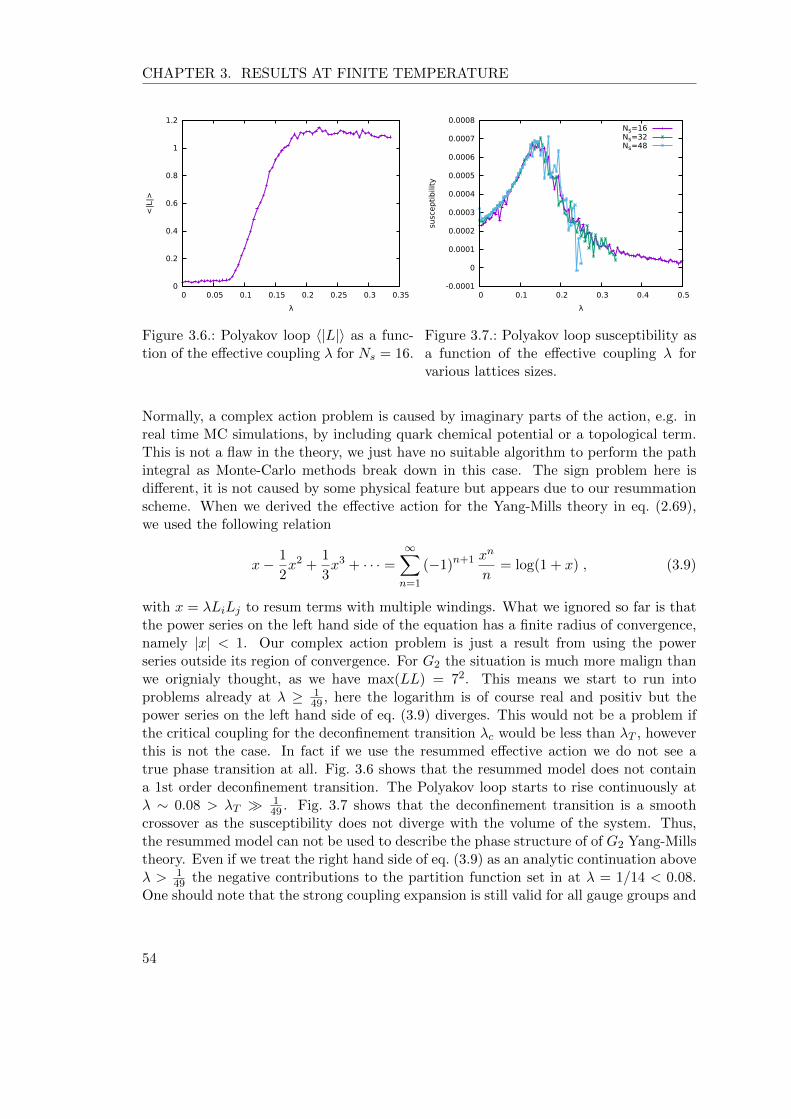
CHAPTER 3. RESULTS AT FINITE TEMPERATURE
0
0.2
0.4
0.6
0.8
1
1.2
0 0.05 0.1 0.15 0.2 0.25 0.3 0.35
<|L
|>
λ
Figure 3.6.: Polyakov loop 〈|L|〉 as a func-tion of the effective coupling λ for Ns = 16.
-0.0001
0
0.0001
0.0002
0.0003
0.0004
0.0005
0.0006
0.0007
0.0008
0 0.1 0.2 0.3 0.4 0.5
susc
epti
bili
ty
λ
Ns=16Ns=32Ns=48
Figure 3.7.: Polyakov loop susceptibility asa function of the effective coupling λ forvarious lattices sizes.
Normally, a complex action problem is caused by imaginary parts of the action, e.g. inreal time MC simulations, by including quark chemical potential or a topological term.This is not a flaw in the theory, we just have no suitable algorithm to perform the pathintegral as Monte-Carlo methods break down in this case. The sign problem here isdifferent, it is not caused by some physical feature but appears due to our resummationscheme. When we derived the effective action for the Yang-Mills theory in eq. (2.69),we used the following relation
x− 1
2x2 +
1
3x3 + · · · =
∞∑n=1
(−1)n+1 xn
n= log(1 + x) , (3.9)
with x = λLiLj to resum terms with multiple windings. What we ignored so far is thatthe power series on the left hand side of the equation has a finite radius of convergence,namely |x| < 1. Our complex action problem is just a result from using the powerseries outside its region of convergence. For G2 the situation is much more malign thanwe orignialy thought, as we have max(LL) = 72. This means we start to run intoproblems already at λ ≥ 1
49 , here the logarithm is of course real and positiv but thepower series on the left hand side of eq. (3.9) diverges. This would not be a problem ifthe critical coupling for the deconfinement transition λc would be less than λT , howeverthis is not the case. In fact if we use the resummed effective action we do not see atrue phase transition at all. Fig. 3.6 shows that the resummed model does not containa 1st order deconfinement transition. The Polyakov loop starts to rise continuously atλ ∼ 0.08 > λT 1
49 . Fig. 3.7 shows that the deconfinement transition is a smoothcrossover as the susceptibility does not diverge with the volume of the system. Thus,the resummed model can not be used to describe the phase structure of of G2 Yang-Millstheory. Even if we treat the right hand side of eq. (3.9) as an analytic continuation aboveλ > 1
49 the negative contributions to the partition function set in at λ = 1/14 < 0.08.One should note that the strong coupling expansion is still valid for all gauge groups and
54
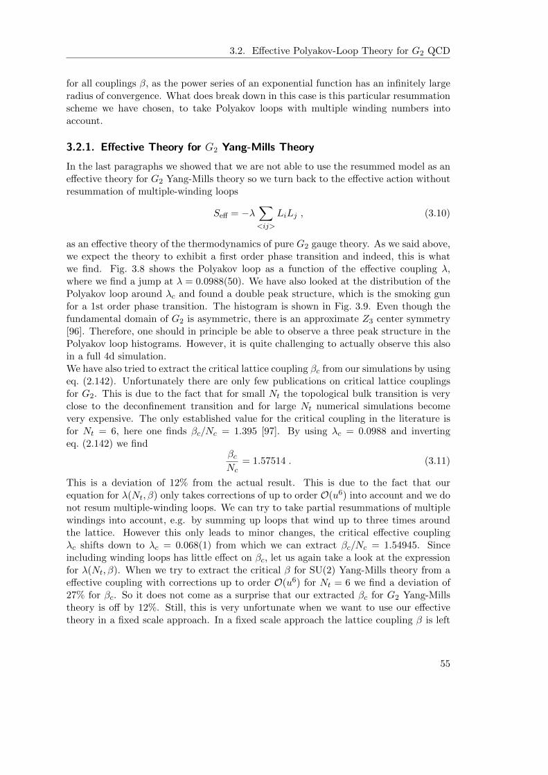
3.2. Effective Polyakov-Loop Theory for G2 QCD
for all couplings β, as the power series of an exponential function has an infinitely largeradius of convergence. What does break down in this case is this particular resummationscheme we have chosen, to take Polyakov loops with multiple winding numbers intoaccount.
3.2.1. Effective Theory for G2 Yang-Mills Theory
In the last paragraphs we showed that we are not able to use the resummed model as aneffective theory for G2 Yang-Mills theory so we turn back to the effective action withoutresummation of multiple-winding loops
Seff = −λ∑<ij>
LiLj , (3.10)
as an effective theory of the thermodynamics of pure G2 gauge theory. As we said above,we expect the theory to exhibit a first order phase transition and indeed, this is whatwe find. Fig. 3.8 shows the Polyakov loop as a function of the effective coupling λ,where we find a jump at λ = 0.0988(50). We have also looked at the distribution of thePolyakov loop around λc and found a double peak structure, which is the smoking gunfor a 1st order phase transition. The histogram is shown in Fig. 3.9. Even though thefundamental domain of G2 is asymmetric, there is an approximate Z3 center symmetry[96]. Therefore, one should in principle be able to observe a three peak structure in thePolyakov loop histograms. However, it is quite challenging to actually observe this alsoin a full 4d simulation.We have also tried to extract the critical lattice coupling βc from our simulations by usingeq. (2.142). Unfortunately there are only few publications on critical lattice couplingsfor G2. This is due to the fact that for small Nt the topological bulk transition is veryclose to the deconfinement transition and for large Nt numerical simulations becomevery expensive. The only established value for the critical coupling in the literature isfor Nt = 6, here one finds βc/Nc = 1.395 [97]. By using λc = 0.0988 and invertingeq. (2.142) we find
βcNc
= 1.57514 . (3.11)
This is a deviation of 12% from the actual result. This is due to the fact that ourequation for λ(Nt, β) only takes corrections of up to order O(u6) into account and we donot resum multiple-winding loops. We can try to take partial resummations of multiplewindings into account, e.g. by summing up loops that wind up to three times aroundthe lattice. However this only leads to minor changes, the critical effective couplingλc shifts down to λc = 0.068(1) from which we can extract βc/Nc = 1.54945. Sinceincluding winding loops has little effect on βc, let us again take a look at the expressionfor λ(Nt, β). When we try to extract the critical β for SU(2) Yang-Mills theory from aeffective coupling with corrections up to order O(u6) for Nt = 6 we find a deviation of27% for βc. So it does not come as a surprise that our extracted βc for G2 Yang-Millstheory is off by 12%. Still, this is very unfortunate when we want to use our effectivetheory in a fixed scale approach. In a fixed scale approach the lattice coupling β is left
55
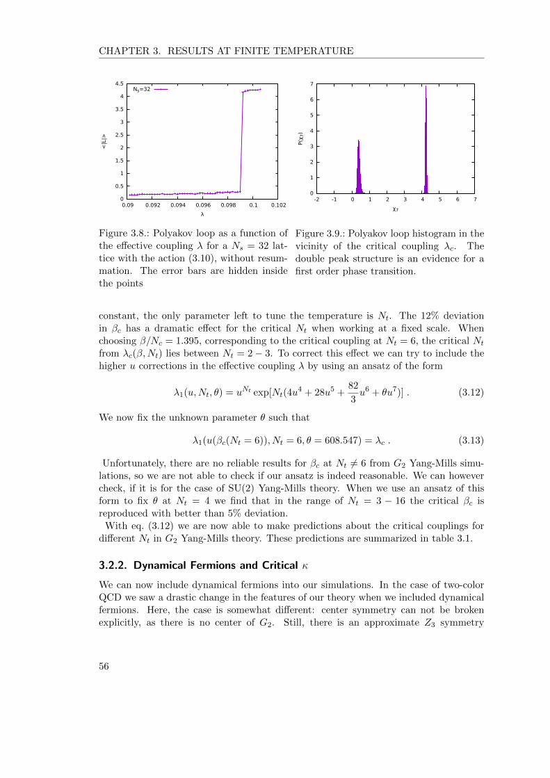
CHAPTER 3. RESULTS AT FINITE TEMPERATURE
0
0.5
1
1.5
2
2.5
3
3.5
4
4.5
0.09 0.092 0.094 0.096 0.098 0.1 0.102
<|L
|>
λ
Ns=32
Figure 3.8.: Polyakov loop as a function ofthe effective coupling λ for a Ns = 32 lat-tice with the action (3.10), without resum-mation. The error bars are hidden insidethe points
0
1
2
3
4
5
6
7
-2 -1 0 1 2 3 4 5 6 7
P(χ
7)
χ7
Figure 3.9.: Polyakov loop histogram in thevicinity of the critical coupling λc. Thedouble peak structure is an evidence for afirst order phase transition.
constant, the only parameter left to tune the temperature is Nt. The 12% deviationin βc has a dramatic effect for the critical Nt when working at a fixed scale. Whenchoosing β/Nc = 1.395, corresponding to the critical coupling at Nt = 6, the critical Nt
from λc(β,Nt) lies between Nt = 2− 3. To correct this effect we can try to include thehigher u corrections in the effective coupling λ by using an ansatz of the form
λ1(u,Nt, θ) = uNt exp[Nt(4u4 + 28u5 +
82
3u6 + θu7)] . (3.12)
We now fix the unknown parameter θ such that
λ1(u(βc(Nt = 6)), Nt = 6, θ = 608.547) = λc . (3.13)
Unfortunately, there are no reliable results for βc at Nt 6= 6 from G2 Yang-Mills simu-lations, so we are not able to check if our ansatz is indeed reasonable. We can howevercheck, if it is for the case of SU(2) Yang-Mills theory. When we use an ansatz of thisform to fix θ at Nt = 4 we find that in the range of Nt = 3 − 16 the critical βc isreproduced with better than 5% deviation.
With eq. (3.12) we are now able to make predictions about the critical couplings fordifferent Nt in G2 Yang-Mills theory. These predictions are summarized in table 3.1.
3.2.2. Dynamical Fermions and Critical κ
We can now include dynamical fermions into our simulations. In the case of two-colorQCD we saw a drastic change in the features of our theory when we included dynamicalfermions. Here, the case is somewhat different: center symmetry can not be brokenexplicitly, as there is no center of G2. Still, there is an approximate Z3 symmetry
56
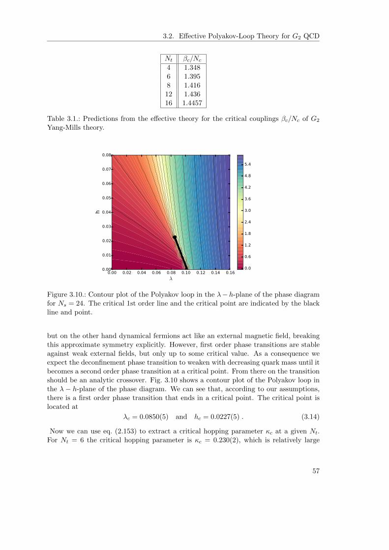
3.2. Effective Polyakov-Loop Theory for G2 QCD
Nt βc/Nc
4 1.3486 1.3958 1.41612 1.43616 1.4457
Table 3.1.: Predictions from the effective theory for the critical couplings βc/Nc of G2
Yang-Mills theory.
0.00 0.02 0.04 0.06 0.08 0.10 0.12 0.14 0.16λ
0.00
0.01
0.02
0.03
0.04
0.05
0.06
0.07
0.08
h
0.0
0.6
1.2
1.8
2.4
3.0
3.6
4.2
4.8
5.4
Figure 3.10.: Contour plot of the Polyakov loop in the λ− h-plane of the phase diagramfor Ns = 24. The critical 1st order line and the critical point are indicated by the blackline and point.
but on the other hand dynamical fermions act like an external magnetic field, breakingthis approximate symmetry explicitly. However, first order phase transitions are stableagainst weak external fields, but only up to some critical value. As a consequence weexpect the deconfinement phase transition to weaken with decreasing quark mass until itbecomes a second order phase transition at a critical point. From there on the transitionshould be an analytic crossover. Fig. 3.10 shows a contour plot of the Polyakov loop inthe λ − h-plane of the phase diagram. We can see that, according to our assumptions,there is a first order phase transition that ends in a critical point. The critical point islocated at
λc = 0.0850(5) and hc = 0.0227(5) . (3.14)
Now we can use eq. (2.153) to extract a critical hopping parameter κc at a given Nt.For Nt = 6 the critical hopping parameter is κc = 0.230(2), which is relatively large
57

CHAPTER 3. RESULTS AT FINITE TEMPERATURE
compared to the critical values for heavy QCD [41]. Unfortunately, there is no datafrom full 4d G2-QCD simulations for the critical κc. However, G2-QCD simulations atκ = 0.1565 in [98] seem to indicate that we have a cross-over at this value of κ [99].We conclude that our equation for the effective fermion coupling h(κ, β,Nt) is not validfor hopping parameters in this range or we need to include additional spatial hoppingterms in the effective action to accurately determine κc. In sec. 4.2 we find evidence thatadditional spatial hopping terms have to be taken into account to reach convergence ofthe hopping series for κ ≈ 0.06 and Nt = 6.
58
4Results at Finite Density
Now, we will turn to the application of the effective theory to the cold and dense partof the phase diagram of QCD-like theories. We will start with results from the effectivetheory for two-color QCD and then discuss results from the effective theory for G2-QCD.
Numerical Details
All our simulations were preformed on NIVIDIA GPUs. Since the effective action isquite complicated we have used the Metropolis algorithm for the update sweeps in oursimulations. For the effective theory for two-color QCD we explicitly made measurementsof the autocorrelations in the density and the Polyakov loop, for that purpose we havegenerated 10 000 configurations. Especially in the transition region between the twoexponential regimes that we are interested in here we find basically no autocorrelations.Only as we approach lattice saturation for µ ≥ mq, see below, we observe some non-negligible autocorrelations in our data. However, for locating the diquark onset and thepseudo-critical values for the Polyakov loop we only use data points at values for thechemical potential of µ ≤ 9.995 GeV where the autocorrelations are negligible. To becompletely safe we nevertheless use only every tenth configuration for the measurementsof the observables, yielding 1000 uncorrelated measurements.
To these measurements we have applied a standard jackknife analysis for the staticalmean and error of our data. The resulting errorbars are included in Fig. 4.1. Becausein linear plots they are always smaller than the symbols, we have omitted them inmost of the other figures with the exception of Fig. 4.9 where we show an example ofthe transition region in close-up with errorbars. In the logarithmic plots the observedscatter of the data at extremely small values of the density or the Polyakov loop serves asan indication of these residual small relative errors from the independent measurements.
In the effective theory for G2-QCD we did not determine the autocorrelations in our
59

CHAPTER 4. RESULTS AT FINITE DENSITY
data, as we expect them to be small when the lattice is not saturated. Still, we usedonly every tenth configuration for the measurements of observables. Again, we omittedthe error bars in the plots, as they are not visible in a linear scale.
4.1. Effective Theory for Two-Color QCD in the Cold andDense Regime
We now turn our attention to the investigation of the cold and dense regime of the two-color QCD phase diagram. Similar to the nuclear liquid-gas transition in QCD thereshould be a phase transition at low temperature and finite baryon chemical potentialto a phase with finite baryon density. In the case of two-color QCD this should be aphase transition to a Bose-Einstein condensate of scalar diquarks, where a non-vanishingdiquark condensate 〈qq〉 6= 0 spontaneously breaks the baryon U(1)B. In contrast toQCD where we have a 1st order liquid-gas phase transition, the phase transition tothe Bose-Einstein condensate is of 2nd order and continuous. Therefore at T = 0 thetransition must occur at µB = md, i.e. µc = md/2 = mπ/2. The BEC is not a self-boundliquid. Thus, the transition happens exactly, when the chemical potential is equal to halfthe diquark mass unlike for the nuclear matter liquid-gas transition, where the criticalµc is shifted by a binding energy µc = mB − ε.
Leading-order mean-field density
Let us start by analyzing the partion function in the strong coupling limit λ = β = 0,where we can solve the integrals for the static part of the fermion determinant analyti-cally. This gives us aditional insight into the model and the effective degrees of freedom.In the strong coupling limit, the partition function factorizes,
Z(β = 0) =
(∫dL [1 + hL+ h2]2Nf × [1 + hL+ h2]2Nf)
N3s
. (4.1)
For T → 0 at a finite chemical Potential µ we have h→ 0. We can now solve the gaugeintegrals analytically, in the case of Nf = 1 we find
Z(β = 0) =
(∫dW [1 + 2h2 + h4 + 2hL+ 2h3L+ h2L2]
)N3s
,
=(1 + 3h2 + h4
)N3s . (4.2)
We see that for Nf = 1 and T → 0, µ > 0 the contributions to the partition function ateach point in space come from diquarks and states consisting of 4 quarks. The Prefactorscan be identified as spin degeneracies, i.e. we have a vector diquark and a scalar 4 quarkstate. This shows us that for Nf = 1 we do not have a scalar diquark and thereforeno Bose-Einstein condensate of scalar diquarks as the groundstate for µ ≥ md/2. For
60
4.1. Effective Theory for Two-Color QCD in the Cold and Dense Regime
Nf=2 the partition function in the strong coupling limit reads
Z(β = 0) =
(∫dL [1 + huL+ h2
u]2 × [1 + hdL+ h2d]
2)N3s
= (1 + 3(h2u + h2
d) + h4u + h4
d + 4huhd + 4(h3uhd + h3
dhu) + 3(h4uh
2d + h4
dh2u)
+ 10h2uh
2d + 4h3
uh3d + h4
uh4d)
N3s
. (4.3)
We can identify the contributions to Z as diquarks and their composites. In particularwe find vector diquarks for all isospin values and an additional scalar diquark in theisopin zero sector. Since we took the trace in Dirac space we can no longer distinguishbetween different parity states but they are degenerate. However from analyzing corre-lators in full two-color QCD we know the theory contains a scalar and a pseudo scalardiquark. Therefore the Nf = 2 theory may have a scalar Bose-Einstein condensate asgroundstate for µ ≥ md/2. Further, we observe an explicit symmetry between flavorsand also between states with 4±n quarks. This second symmetry leads to a particle-holesymmetry around the half-filling point of the lattice.Since all our simulations are done on a lattice with a finite size we will always encountera finite expectation value of the Polyakov loop. To include this finite volume artifact wewill use eq. (4.1) with mean-field description for the Polyakov loop. At T → 0, µ > 0the partition functions reads
Z = [1 + 2hL+ h2]2NfN3s , (4.4)
where a factor of two was inserted because the mean-field Polyakov loop L here isnormalized to assume values within [−1, 1]. The quark number density then follows as
n =T
V
∂
∂µlnZ ,
a3n = 4Nf1 + Le
mq−µT
1 + 2Lemq−µT + e
2(mq−µ)
T
. (4.5)
The same expression can be derived from a Polyakov-Quark-Meson-Diquark model [53]for very heavy quarks where the quark mass is larger than the UV cutoff Λ. For L = 1 itsimply reduces to the zero-momentum occupation number of the Fermi-Dirac distribu-tion since the momentum is negligible compared to the mass m2 p2. In the deconfinedphase it thus describes a free gas of heavy quarks. In the confined phase with L = 0statistical confinement rules out single quark states and we only find states with integerbaryon numbers. We will see below that for small but finite Polyakov-loop expectationvalues L > 0, and small T , Eq. (4.5) due to imperfect confinement behaves as a quarkgas, suppressed by L, up to some critical chemical potential µc(T ) where it starts to re-flect the behavior of a diquark gas with md = 2mq at this leading-order. By consideringµ < mq and hence x ≡ exp(mq − µ)/T > 1, we can then distinguish two regimes:
a3n
4Nf→
e(µB−md)/T , L x 1 ,
L e(µ−mq)/T , L x 1 .(4.6)
61
CHAPTER 4. RESULTS AT FINITE DENSITY
The transition occurs at around L x ∼ 1 or respectively µc ∼ mq + T ln L .
Scale Setting and Units
Of course we could state all our results in terms of the lattice spacing a. However to havea more intuitive view on the results we will set a scale and give our results in naturalunits. The first thing to do is to set a scale. We will assume that quarks as heavy asthose used here only have a negligible influence on the running of the coupling, thereforewe use the non-perturbative SU(2) Yang-Mills β-function from [92]
1
a√σ
= exp
(β − db
), (4.7)
with the parametersd = 1.98(1) , b = 0.305(6) . (4.8)
In lack of phenomenological input we somewhat arbitrarily use the typical√σ = 440 MeV
from QCD also for the string tension of two-color QCD. With Eqs. (4.7) and (2.131)we are then able to assign a physical scale to our systems. In all our simulations thediquark mass from Eq. (2.131) is adjusted in this way to md = 20 GeV, and the tem-peratures range between T = 3.454 MeV and 9 MeV. On our finest lattice with β = 2.5,corresponding to a = 0.0810 fm, this amounts to κ = 0.00802123 and Nt values between269 and 700. The parameters for the coarser lattices with β values down to 2.4 lead toeven smaller values for the expansion parameter.
Convergence of the hopping series
In order to assess the range of validity of the effective theory we need to test the conver-gence properties of the hopping series for various parameter choices. As can be seen fromEquation (2.127) the relevant expansion parameter for the effective theory is κ2Nt/Nc.Because we are interested in very low temperatures T = 1/aNt, we need lattices of largeextend Nt in the temporal direction, especially as we go to smaller lattice spacings a.Therefore our hopping parameter κ needs to be sufficiently small. This implies that onecan reach smaller quark masses at higher temperatures and vice versa. To check theconvergence of the hopping expansion we compare expectation values for the densitiesa3n from simulations including corrections up to O(κ2) and O(κ4) for different values of
the expansion parameter κ2NtNc
. By taking a closer look at the effective action (2.127) onerecognizes that the convergence properties of the hopping series change with chemicalpotential µ. For small chemical potentials we have h→ 0 and all O(κ2Nt/Nc) correctionsbecome negligible. For large chemical potentials we have h→∞ and all all O(κ2Nt/Nc)corrections become zero or constant and therefore also negligible. The effect of the cor-rections is most prominent when h is of order 1 or respectively µ = md/2, which is wherewe should check the convergence properties of the hopping series. Figure 4.1 shows aplot of the two densities for µ = md/2 at β = 2.5, including gauge corrections. The twoagree reasonably well for all values of κ2Nt/2 up to slightly above 0.02. Our Nt range of269 to 700 is chosen such that κ2Nt/2 lies within 0.0087 and 0.0225, and hence within
62
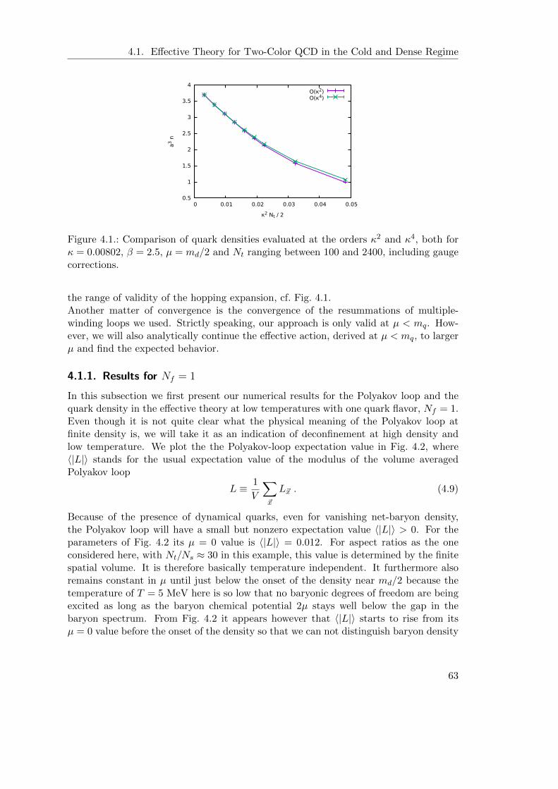
4.1. Effective Theory for Two-Color QCD in the Cold and Dense Regime
0.5
1
1.5
2
2.5
3
3.5
4
0 0.01 0.02 0.03 0.04 0.05
a3 n
κ2 Nt / 2
O(κ2)O(κ4)
Figure 4.1.: Comparison of quark densities evaluated at the orders κ2 and κ4, both forκ = 0.00802, β = 2.5, µ = md/2 and Nt ranging between 100 and 2400, including gaugecorrections.
the range of validity of the hopping expansion, cf. Fig. 4.1.Another matter of convergence is the convergence of the resummations of multiple-winding loops we used. Strictly speaking, our approach is only valid at µ < mq. How-ever, we will also analytically continue the effective action, derived at µ < mq, to largerµ and find the expected behavior.
4.1.1. Results for Nf = 1
In this subsection we first present our numerical results for the Polyakov loop and thequark density in the effective theory at low temperatures with one quark flavor, Nf = 1.Even though it is not quite clear what the physical meaning of the Polyakov loop atfinite density is, we will take it as an indication of deconfinement at high density andlow temperature. We plot the the Polyakov-loop expectation value in Fig. 4.2, where〈|L|〉 stands for the usual expectation value of the modulus of the volume averagedPolyakov loop
L ≡ 1
V
∑~x
L~x . (4.9)
Because of the presence of dynamical quarks, even for vanishing net-baryon density,the Polyakov loop will have a small but nonzero expectation value 〈|L|〉 > 0. For theparameters of Fig. 4.2 its µ = 0 value is 〈|L|〉 = 0.012. For aspect ratios as the oneconsidered here, with Nt/Ns ≈ 30 in this example, this value is determined by the finitespatial volume. It is therefore basically temperature independent. It furthermore alsoremains constant in µ until just below the onset of the density near md/2 because thetemperature of T = 5 MeV here is so low that no baryonic degrees of freedom are beingexcited as long as the baryon chemical potential 2µ stays well below the gap in thebaryon spectrum. From Fig. 4.2 it appears however that 〈|L|〉 starts to rise from itsµ = 0 value before the onset of the density so that we can not distinguish baryon density
63

CHAPTER 4. RESULTS AT FINITE DENSITY
0
0.5
1
1.5
2
2.5
3
3.5
4
9.9 9.92 9.94 9.96 9.98 10 10.02 0
0.1
0.2
0.3
0.4
0.5
0.6
0.7
0.8
0.9
a3n
<|L
|>
µ in GeV
a3n<|L|>
Figure 4.2.: Quark density a3n in latticeunits and Polyakov-loop expectation value〈|L|〉, both over µ, with simulation param-eters β = 2.5, κ = 0.00802, leading tomd = 20 GeV, Ns = 16, Nt = 484, cor-responding to T = 5 MeV, and Nf = 1.
0
2
4
6
8
10
9.99 9.995 10 10.005
T in M
eV
µ in GeV
pseudo-critical pointsdeconfinement
Figure 4.3.: The pseudo-critical line for thedeconfinement transition from simulationswith the same parameters as in Fig. 4.2except for different Nt, corresponding toT = 9, 8, . . . 4 MeV and 3.454 MeV, witha linear extrapolation to T = 0.
from quark density here. As we will discuss in the next subsection, however, there is avery small diquark contribution in the density above µc ≈ 9.96 GeV at this temperaturewhich is not visible on the linear scale of Fig. 4.2 but where the Polyakov loop still has itszero-density expectation value. We will provide some evidence that this diquark-densityonset might stay below the deconfinement transition when we extrapolate both to T = 0for Nf = 2 with scalar diquarks below.
At larger values of the chemical potential the quark density saturates at a3n = 2NcNf .This is the maximum number of quarks per site due to the Pauli principle, as in theeffective theory for heavy quarks in SU(3) [40]. This behavior which is a lattice artifacthas previously also been observed in finite density simulations of two-color [47] andG2-QCD [98]. This saturation leads to an effective quenching of the quarks and hencethe Polyakov loop decreases again as it is approached. We also analyzed the Polyakov-loop susceptibility and found no increase of its rather broad maximum with the latticevolume hence indicating a smooth cross-over behavior rather than a deconfinement phasetransition in the infinite volume limit. The pseudo-critical chemical potential µpc fromthe inflection point of 〈|L|〉 along the µ axis is shown in Fig. 4.3. It coincides withthe point where 〈|L|〉 reaches half its maximum value. By determining this µpc fordifferent temperatures we obtain a pseudo-critical line for the deconfiment transition atlow temperature which can be extrapolated to T = 0 as shown in Fig. 4.3. We can seethat the pseudo-critical line terminates at µpc slightly above 10 GeV which correspondsto half the scalar-diquark mass from eq. (2.140) with the parameters used here.
We conclude this subsection by discussing in some more detail the quark-number
64
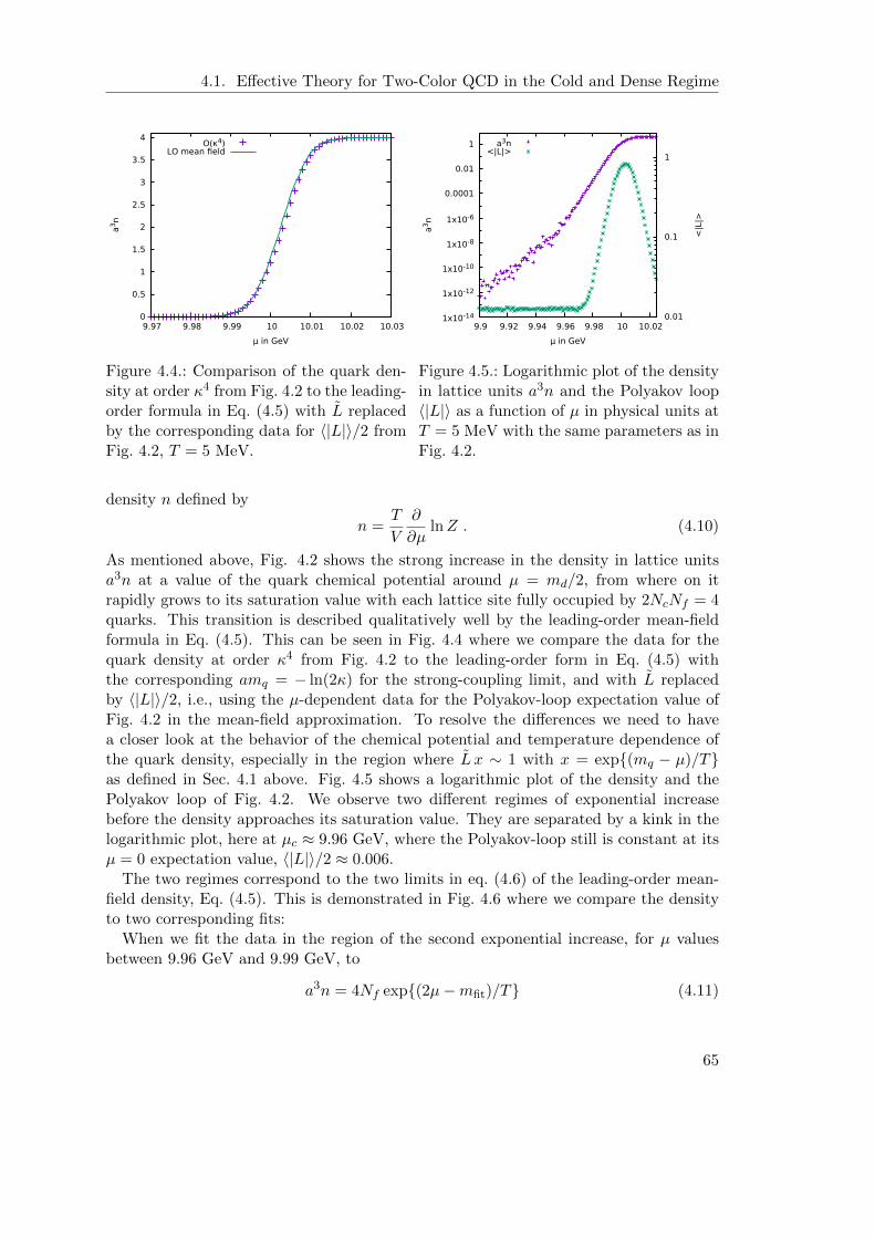
4.1. Effective Theory for Two-Color QCD in the Cold and Dense Regime
0
0.5
1
1.5
2
2.5
3
3.5
4
9.97 9.98 9.99 10 10.01 10.02 10.03
a3n
µ in GeV
O(κ4)LO mean field
Figure 4.4.: Comparison of the quark den-sity at order κ4 from Fig. 4.2 to the leading-order formula in Eq. (4.5) with L replacedby the corresponding data for 〈|L|〉/2 fromFig. 4.2, T = 5 MeV.
1x10-14
1x10-12
1x10⁻¹⁰
1x10⁻⁸
1x10⁻⁶
0.0001
0.01
1
9.9 9.92 9.94 9.96 9.98 10 10.02 0.01
0.1
1
a3n
<|L
|>
µ in GeV
a3n<|L|>
Figure 4.5.: Logarithmic plot of the densityin lattice units a3n and the Polyakov loop〈|L|〉 as a function of µ in physical units atT = 5 MeV with the same parameters as inFig. 4.2.
density n defined by
n =T
V
∂
∂µlnZ . (4.10)
As mentioned above, Fig. 4.2 shows the strong increase in the density in lattice unitsa3n at a value of the quark chemical potential around µ = md/2, from where on itrapidly grows to its saturation value with each lattice site fully occupied by 2NcNf = 4quarks. This transition is described qualitatively well by the leading-order mean-fieldformula in Eq. (4.5). This can be seen in Fig. 4.4 where we compare the data for thequark density at order κ4 from Fig. 4.2 to the leading-order form in Eq. (4.5) withthe corresponding amq = − ln(2κ) for the strong-coupling limit, and with L replacedby 〈|L|〉/2, i.e., using the µ-dependent data for the Polyakov-loop expectation value ofFig. 4.2 in the mean-field approximation. To resolve the differences we need to havea closer look at the behavior of the chemical potential and temperature dependence ofthe quark density, especially in the region where L x ∼ 1 with x = exp(mq − µ)/Tas defined in Sec. 4.1 above. Fig. 4.5 shows a logarithmic plot of the density and thePolyakov loop of Fig. 4.2. We observe two different regimes of exponential increasebefore the density approaches its saturation value. They are separated by a kink in thelogarithmic plot, here at µc ≈ 9.96 GeV, where the Polyakov-loop still is constant at itsµ = 0 expectation value, 〈|L|〉/2 ≈ 0.006.
The two regimes correspond to the two limits in eq. (4.6) of the leading-order mean-field density, Eq. (4.5). This is demonstrated in Fig. 4.6 where we compare the densityto two corresponding fits:
When we fit the data in the region of the second exponential increase, for µ valuesbetween 9.96 GeV and 9.99 GeV, to
a3n = 4Nf exp(2µ−mfit)/T (4.11)
65

CHAPTER 4. RESULTS AT FINITE DENSITY
1x10
1x10
1x10
1x10
1
9.88 9.9 9.92 9.94 9.96 9.98 10 10.02
an
µ in GeV
a n
4 Nf L exp
(
µ−mq
T
)
4Nf exp(
2µ−md
T
)
Figure 4.6.: Logarithmic plot of the den-sity in lattice units a3n at T = 5 MeVcompared to one-parameter fits using L forµ < 9.96 GeV and md for µ > 9.96 GeV,see text.
1x10-18
1x10-16
1x10-14
1x10-12
1x10⁻¹⁰
1x10⁻⁸
1x10⁻⁶
0.0001
0.01
1
100
9.88 9.9 9.92 9.94 9.96 9.98 10 10.02
a3n
µ in GeV
4 MeV6 MeV9 MeV
Figure 4.7.: Comparison of the measureddensity with the leading-order mean-fielddensity with L = 〈L~x〉/2 at md = 20 GeV,β = 2.5, κ = 0.00802, and different temper-atures.
with a single parameter mfit we obtain for Nf = 1,
mfit = 20.0045(5) GeV . (4.12)
For comparison, with the same lattice parameters the quark mass from Eq. (2.89) be-
comes m(0)q = 10.0024 GeV at the leading-order n+m = 0, m
(4)q = 10.0014 GeV at the
order n + m = 4, and m(7)q = 10.0013 GeV at the order n + m = 7. Therefore, the fit
parameter mfit is consistent with 2m(0)q but slightly larger than 2mq = 20.0028(2) at the
same order n + m = 4 (with an error of the size of the higher-order corrections up ton + m = 7 as given explicitly in Eq. (2.89)). It is larger than the corresponding scalardiquark mass, md = 20 GeV from Eq. (2.140), which might simply reflect the fact thatscalar diquarks do not exist for Nf = 1. A daring interpretation would be that we see aheavier diquark mass here, such as that of an axial-vector diquark which can exist alsofor Nf = 1.
To test this, we have done the same analysis with the same parameters also for twoflavors (see the next subsection). The same fit to the form in (4.11) then yields forNf = 2,
mfit = 19.9986(10) GeV , (4.13)
which is now indeed very close to the scalar diquark mass md and significantly smallerthan 2mq. In order to quantitatively describe this regime of exponential increase wetherefore have to replace 2mq by md in the leading-order mean-field formula for thedensity in Eq. (4.5). This indicates that matter on this side of the kink consists ofdiquark excitations.
The first exponential increase, for the µ values below 9.96 GeV, is described by
a3n = 4Nf L exp(µ−mq)/T . (4.14)
66

4.1. Effective Theory for Two-Color QCD in the Cold and Dense Regime
In this case we use mq = 10.0014 GeV for the quark mass at this order and fit the datavia L as the free parameter. For the one-flavor data of Fig. 4.6 this leads to L of theorder of 10−4, however, with a very large uncertainty. It determines the precise valueof the onset µc of the diquark density, by the intersection point of the two differentexponential fits (4.11) and (4.14), as
L = exp(µc −md +mq)/T . (4.15)
With md = mfit from (4.12) for the Nf = 1 data in Fig. 4.6, for example, this leads tovalues between L = 8 · 10−5 for µc = 9.956 GeV and L = 1.2 · 10−4 for µc = 9.958 GeV.In any case, it is much smaller than the zero-density value of 〈|L|〉/2 ≈ 0.006. Instead weobserve that it is more consistent with the expectation value of the local Polyakov loopL~x. Its expectation value is extracted from the per-site probability distribution P (L~x)which we obtain by histograming the local Polyakov-loop variable L~x as in [92]. At T = 5MeV, with β = 2.5 and κ = 0.00802, we obtain for this observable a zero-density valueof about 〈L~x〉 ∼ 10−4 instead of 〈|L|〉 ≈ 0.012 for the modulus of the volume-averagedPolyakov loop. This suggests that one should use the local Polyakov-loop expectationvalue 〈L~x〉 in mean-field approximations as Eq (4.5). The reason behind this can be foundby analyzing values of the local Polyakov loop: since the probability distribution of thelocal Polyakov loops stays symmetric around zero up to µpc we will always have somenegative Polyakov loops. A quick look at eq. (4.5) shows that a negative local Polyakovloop induces negative local particle numbers. Now the expectation value 〈L~x〉 stayspositiv but using 〈|L|〉 as mean-field Polyakov loop value completly ignores the negativecontributions and therefore overestimates the density. Like 〈|L|〉, 〈L~x〉 is independentof the chemical potential below the deconfinement crossover at µpc. And as soon asthe Polyakov-loop starts to rise from its constant zero-density expectation value the twoagree well within the errors. It is only the residual small value at vanishing net-baryondensity due to imperfect confinement in a finite volume in which the two differ simplybecause it takes longer for the modulus to vanish than the local Polyakov loop in theinfinite-volume limit for µ < µpc. This difference is only relevant at densities in latticeunits below 10−4 and hence not visible on the linear scale of Fig. 4.4 above.
In fact, using the local Polyakov-loop expectation value 〈L~x〉 for various temperaturesin the leading-order mean-field formula for the quark density, Eq. (4.5), describes thedata especially also in the low-density region around the diquark-density onset at µcvery well as can be seen in Fig. 4.7. These are not fits. We simply use Eq. (4.5) withL = 〈L~x〉/2 here to describe the quark density over the whole range of temperatureswe have investigated. It describes the imperfect statistical confinement of quarks for µbelow µc = md−mq+T ln(〈L~x〉/2), an ensemble of diquarks above µc, and quark matterwith lattice saturation for µ larger than µpc where 2L = 〈L~x〉 = 〈|L|〉 as in Fig. 4.4, allat the same time.
4.1.2. Results for Nf = 2
In this subsection we discuss the results from the effective theory with Nf = 2 degeneratequark flavors in somewhat more detail. In particular, we describe how well the onset of
67

CHAPTER 4. RESULTS AT FINITE DENSITY
0
1
2
3
4
5
6
7
8
9.9 9.92 9.94 9.96 9.98 10 10.02 0
0.2
0.4
0.6
0.8
1
1.2
a3n
<|L
|>
µ in GeV
a3n<|L|>
Figure 4.8.: Quark density in lattice unitsand Polyakov-loop expectation value 〈|L|〉,both over µ, with the same simulation pa-rameters as in Fig. 4.2, but for Nf = 2 here.
0
5x10⁻⁶
1x10⁻⁵
1.5x10⁻⁵
2x10⁻⁵
2.5x10⁻⁵
9.95 9.955 9.96 9.965 9.97
a3n8 exp((2µ-md)/T)
Figure 4.9.: Zoom-in of Fig. 4.8 on the re-gion of the diquark onset. Also shown is thefit to the LO mean-field formula for the sec-ond exponential increase from Eq. (4.11).
the diquark density at µ = µc agrees with the scalar diquark mass md from Eq. (2.140)which we know exists for Nf = 2.
As a first example in Fig. 4.8 we present the Nf = 2 results for the quark densityand the Polyakov loop on our finest lattice, with β = 2.5, κ = 0.00802123, Ns = 16and Nt = 484. This set of parameters corresponds to md = 20 GeV and T = 5 MeV ata lattice spacing of a = 0.081 fm as in the previous subsection for the one-flavor case.Both observables show the same qualitative behavior as for Nf = 1 before.
The most obvious differences between Nf = 1 and 2 are the different saturationdensities given by a3nsat = 2NcNf and the maximum value of the Polyakov loop 〈|L|〉which is a bit higher for Nf = 2. The direct comparison of the Polyakov-loop expectationvalues in Fig. 4.10 shows that the deconfinement crossover tends to start at somewhatsmaller values of µ for Nf = 2, and gets quenched later, likewise.
The difference between the normalized quark-number densities n/nsat for Nf = 2 andNf = 1 is shown in Fig. 4.11. We can see a deviation around µ = 10 GeV. This is inline with the observation that the deconfinement transition happens earlier for Nf = 2as well. As described for Nf = 1 above, we follow the same procedure with Nf = 2 forvarious temperatures from 9 MeV down to 3.454 MeV. That is, for each temperature wedetermine the intersection point of the two exponential regimes in the quark density (forNf = 2 their µ-values are consistently about 1 − 2 MeV lower than those for Nf = 1).Since the mass-parameter in the second exponential for Nf = 2, see Eq. (4.13), agreeswell with the scalar diquark mass, md = 20 GeV from Eq. (2.140), we now take theintersection of the lines in logarithmic plots analogous to Fig. 4.6 as the onset of baryonicdiquark matter and extrapolate the corresponding onset chemical potentials µc to T = 0.The result for the Ns = 16 lattice is shown in Fig. 4.12. Using a linear extrapolationas in the figure, which is consistent with a temperature independent L ≈ 〈L〉/2, the
68
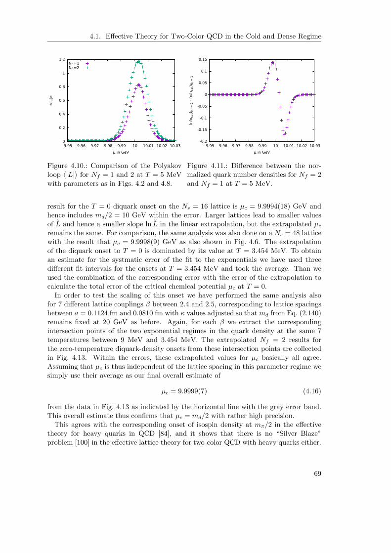
4.1. Effective Theory for Two-Color QCD in the Cold and Dense Regime
0
0.2
0.4
0.6
0.8
1
1.2
9.95 9.96 9.97 9.98 9.99 10 10.01 10.02 10.03
<|L
|>
µ in GeV
Nf =1Nf =2
Figure 4.10.: Comparison of the Polyakovloop 〈|L|〉 for Nf = 1 and 2 at T = 5 MeVwith parameters as in Figs. 4.2 and 4.8.
-0.2
-0.15
-0.1
-0.05
0
0.05
0.1
0.15
9.95 9.96 9.97 9.98 9.99 10 10.01 10.02 10.03
(n/n
sat)
Nf =
2 -
(n/n
sat)
Nf =
1
µ in GeV
Figure 4.11.: Difference between the nor-malized quark number densities for Nf = 2and Nf = 1 at T = 5 MeV.
result for the T = 0 diquark onset on the Ns = 16 lattice is µc = 9.9994(18) GeV andhence includes md/2 = 10 GeV within the error. Larger lattices lead to smaller valuesof L and hence a smaller slope ln L in the linear extrapolation, but the extrapolated µcremains the same. For comparison, the same analysis was also done on a Ns = 48 latticewith the result that µc = 9.9998(9) GeV as also shown in Fig. 4.6. The extrapolationof the diquark onset to T = 0 is dominated by its value at T = 3.454 MeV. To obtainan estimate for the systmatic error of the fit to the exponentials we have used threedifferent fit intervals for the onsets at T = 3.454 MeV and took the average. Than weused the combination of the corresponding error with the error of the extrapolation tocalculate the total error of the critical chemical potential µc at T = 0.
In order to test the scaling of this onset we have performed the same analysis alsofor 7 different lattice couplings β between 2.4 and 2.5, corresponding to lattice spacingsbetween a = 0.1124 fm and 0.0810 fm with κ values adjusted so that md from Eq. (2.140)remains fixed at 20 GeV as before. Again, for each β we extract the correspondingintersection points of the two exponential regimes in the quark density at the same 7temperatures between 9 MeV and 3.454 MeV. The extrapolated Nf = 2 results forthe zero-temperature diquark-density onsets from these intersection points are collectedin Fig. 4.13. Within the errors, these extrapolated values for µc basically all agree.Assuming that µc is thus independent of the lattice spacing in this parameter regime wesimply use their average as our final overall estimate of
µc = 9.9999(7) (4.16)
from the data in Fig. 4.13 as indicated by the horizontal line with the gray error band.This overall estimate thus confirms that µc = md/2 with rather high precision.
This agrees with the corresponding onset of isospin density at mπ/2 in the effectivetheory for heavy quarks in QCD [84], and it shows that there is no “Silver Blaze”problem [100] in the effective lattice theory for two-color QCD with heavy quarks either.
69

CHAPTER 4. RESULTS AT FINITE DENSITY
0
2
4
6
8
10
9.9 9.92 9.94 9.96 9.98 10 10.02
T in M
eV
µ in GeV
linear extrapolation Ns=16onset points Ns=16
linear extrapolation Ns=48onset points Ns=48
Figure 4.12.: Section of the Nf = 2 phase diagram with a linear extrapolation of thediquark-density onset to T = 0 at β = 2.5 or a = 0.081 fm with Ns = 16 and Ns = 48.
In contrast to the effective theory for heavy quarks in QCD [84] where there is someevidence of a finite binding energy per nucleon ε, shifting the nuclear-matter transitionto 3µc = mB − ε, there is no such evidence of a shift of the onset µc by a non-zero εin the effective theory for heavy two-color QCD. This is consistent with the generallyexpected difference between a first-order liquid-gas transition in QCD and Bose-Einsteincondensation of diquarks in a second-order transition in two-color QCD. At the sametime, however, the diquark densities obtained here are far from reflecting any sign ofBose-Einstein condensation. Quarks and diquarks are way too heavy to interpret thelatter as deeply bound dimers. With our parameters for the β = 2.5 lattice the 20 GeVdiquarks are only bound by about 2.8 MeV. If it wasn’t for confinement, the transitiontemperature of the diquark-condensation phase by pair breaking should roughly be of thesame order. All we can observe here is an essentially free heavy-diquark gas behavior inthe small window between µ = µc(T ) and the beginning deconfinement crossover followedby lattice saturation. The only reason we can observe this diquark gas at temperaturesabove 4 MeV is probably statistical confinement. Unfortunately, the region where onemight find a superfluid diquark-condensation phase is currently still beyond reach withinthe convergence region of the hopping series. Nevertheless, we can attempt to give avery rough first estimate of a region where such a diquark superfluid might be found, ifwe were able to further reduce the temperature, as follows:
Since the pseudo-critical chemical potentials for deconfinement at the available tem-peratures are also all below md/2, we compare their zero-temperature extrapolation tothat of the diquark-density onset in Fig. 4.14. The difference between the extrapolatedµc = md/2 and µpc is small but significant. As seen in the figure, the deconfinementcrossover then hits the T = 0 axis of the phase diagram just above mq = 10.0014 GeV.Therefore, a small window for a potential superfluid diquark-condensation phase at suf-ficiently low temperatures remains. The region where this might occur is indicated bythe shaded red triangle in Fig. 4.14. This region starts at a chemical potential slightlybelow µ = md/2 = 10 GeV, i.e. at the lower limit given by the extrapolation error of the
70
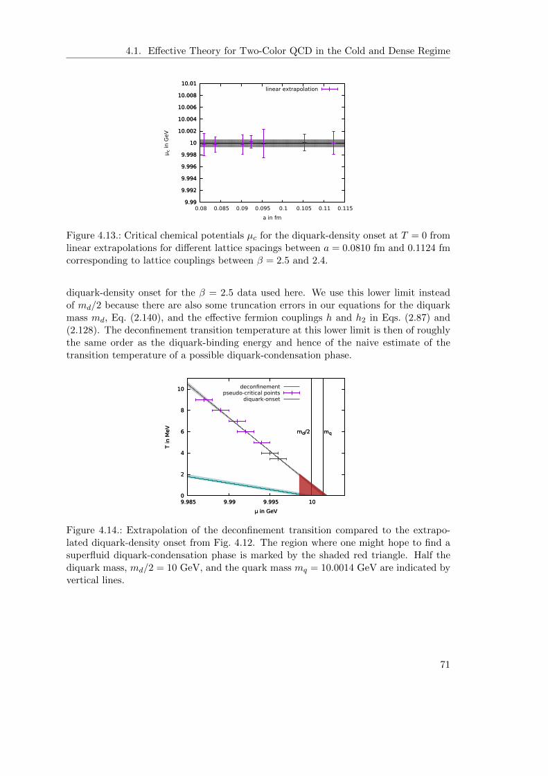
4.1. Effective Theory for Two-Color QCD in the Cold and Dense Regime
9.99
9.992
9.994
9.996
9.998
10
10.002
10.004
10.006
10.008
10.01
9.99
9.992
9.994
9.996
9.998
10
10.002
10.004
10.006
10.008
10.01
0.08 0.085 0.09 0.095 0.1 0.105 0.11 0.115
µc
in G
eV
a in fm
linear extrapolation
Figure 4.13.: Critical chemical potentials µc for the diquark-density onset at T = 0 fromlinear extrapolations for different lattice spacings between a = 0.0810 fm and 0.1124 fmcorresponding to lattice couplings between β = 2.5 and 2.4.
diquark-density onset for the β = 2.5 data used here. We use this lower limit insteadof md/2 because there are also some truncation errors in our equations for the diquarkmass md, Eq. (2.140), and the effective fermion couplings h and h2 in Eqs. (2.87) and(2.128). The deconfinement transition temperature at this lower limit is then of roughlythe same order as the diquark-binding energy and hence of the naive estimate of thetransition temperature of a possible diquark-condensation phase.
0
2
4
6
8
10
9.985 9.99 9.995 10
md/2 mq
T in M
eV
µ in GeV
deconfinementpseudo-critical points
diquark-onset
0
2
4
6
8
10
9.985 9.99 9.995 10
md/2 mq
T in M
eV
µ in GeV
Figure 4.14.: Extrapolation of the deconfinement transition compared to the extrapo-lated diquark-density onset from Fig. 4.12. The region where one might hope to find asuperfluid diquark-condensation phase is marked by the shaded red triangle. Half thediquark mass, md/2 = 10 GeV, and the quark mass mq = 10.0014 GeV are indicated byvertical lines.
71
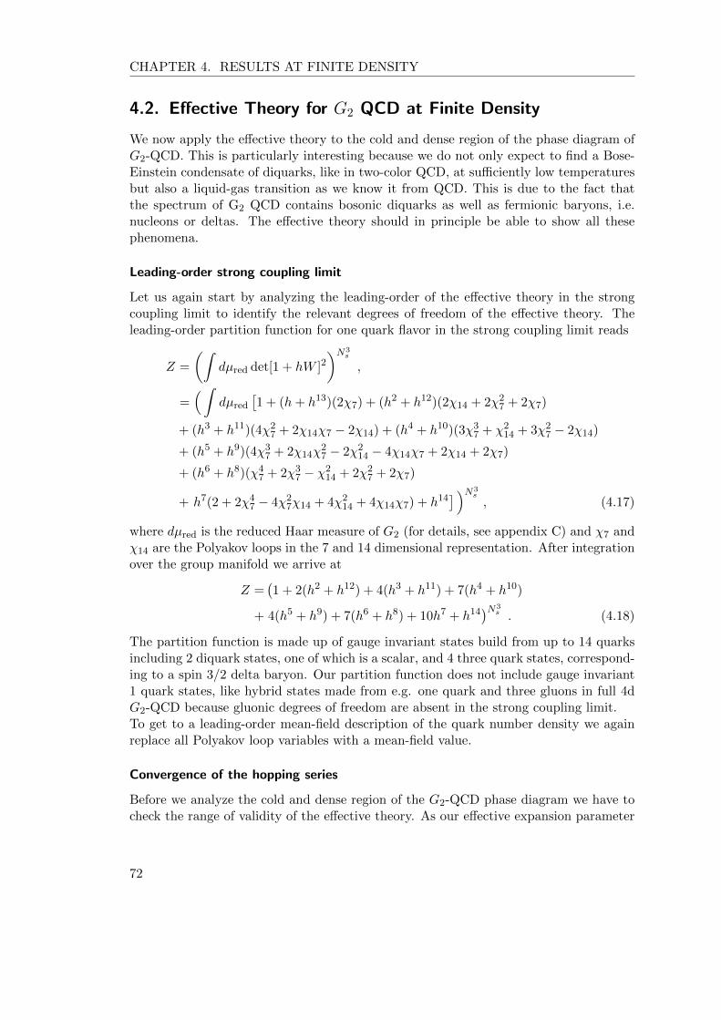
CHAPTER 4. RESULTS AT FINITE DENSITY
4.2. Effective Theory for G2 QCD at Finite Density
We now apply the effective theory to the cold and dense region of the phase diagram ofG2-QCD. This is particularly interesting because we do not only expect to find a Bose-Einstein condensate of diquarks, like in two-color QCD, at sufficiently low temperaturesbut also a liquid-gas transition as we know it from QCD. This is due to the fact thatthe spectrum of G2 QCD contains bosonic diquarks as well as fermionic baryons, i.e.nucleons or deltas. The effective theory should in principle be able to show all thesephenomena.
Leading-order strong coupling limit
Let us again start by analyzing the leading-order of the effective theory in the strongcoupling limit to identify the relevant degrees of freedom of the effective theory. Theleading-order partition function for one quark flavor in the strong coupling limit reads
Z =
(∫dµred det[1 + hW ]2
)N3s
,
=(∫
dµred
[1 + (h+ h13)(2χ7) + (h2 + h12)(2χ14 + 2χ2
7 + 2χ7)
+ (h3 + h11)(4χ27 + 2χ14χ7 − 2χ14) + (h4 + h10)(3χ3
7 + χ214 + 3χ2
7 − 2χ14)
+ (h5 + h9)(4χ37 + 2χ14χ
27 − 2χ2
14 − 4χ14χ7 + 2χ14 + 2χ7)
+ (h6 + h8)(χ47 + 2χ3
7 − χ214 + 2χ2
7 + 2χ7)
+ h7(2 + 2χ47 − 4χ2
7χ14 + 4χ214 + 4χ14χ7) + h14
] )N3s, (4.17)
where dµred is the reduced Haar measure of G2 (for details, see appendix C) and χ7 andχ14 are the Polyakov loops in the 7 and 14 dimensional representation. After integrationover the group manifold we arrive at
Z =(1 + 2(h2 + h12) + 4(h3 + h11) + 7(h4 + h10)
+ 4(h5 + h9) + 7(h6 + h8) + 10h7 + h14)N3
s . (4.18)
The partition function is made up of gauge invariant states build from up to 14 quarksincluding 2 diquark states, one of which is a scalar, and 4 three quark states, correspond-ing to a spin 3/2 delta baryon. Our partition function does not include gauge invariant1 quark states, like hybrid states made from e.g. one quark and three gluons in full 4dG2-QCD because gluonic degrees of freedom are absent in the strong coupling limit.To get to a leading-order mean-field description of the quark number density we againreplace all Polyakov loop variables with a mean-field value.
Convergence of the hopping series
Before we analyze the cold and dense region of the G2-QCD phase diagram we have tocheck the range of validity of the effective theory. As our effective expansion parameter
72

4.2. Effective Theory for G2 QCD at Finite Density
4
4.5
5
5.5
6
6.5
0 0.001 0.002 0.003 0.004 0.005 0.006 0.007 0.008
a3 n
κ2 Nt / 7
O(κ2)O(κ4)
Figure 4.15.: Comparison of quark densities evaluated at the orders κ2 and κ4, both forκ = 0.005, β/Nc = 1.39, µ = md/2 and Nt ranging between 100 and 2000, includinggauge corrections.
is κ2Nt/Nc, we will vary this parameter and compare results of simulations includingcorrections up to order O(κ2) and O(κ4). This way we can check the convergence of thehopping series. The effects of the corrections are largest when h is of order one. Fig. 4.15shows a plot of the two quark number densities for β/Nc = 1.39, µ = md/2, includinggauge corrections. The two curves agree up to κ2Nt/Nc ≈ 0.003. If we compare thisto the results for the effective action for two-color QCD in Fig. 4.1, we see that theconvergence region for the effective theory for G2 is much smaller. Even for small valuesof Nt, we have to choose κ very small to ensure convergence.
4.2.1. Results
Let us start by discussing results for the Polyakov loop and quark number density for lowtemperatures and one quark flavor. We choose our parameters such that we are certainto stay in the convergence region of the hopping expansion. Fig. 4.16 shows the quarknumber density and the Polyakov loop expectation value of the fundamental representa-tions for the parameter set: β/Nc = 1.39, κ = 0.005, leading to amd = 9.210, Nt = 100and Nf = 1. In this case, the effective expansion parameter is κ2Nt/Nc = 3.6 · 10−4
and thus well inside the convergence region. We again see that the quark number densityand the Polyakov-loop stay almost zero and independent of µ until the chemical potentialapproaches half the diquark mass µ ≈ md/2. Beyond that point we see a sharp increasein the quark number density until it saturates at 2 ·Nc = 14, as expected. The Polyakov-loop also starts to rise as µ is approaching md/2, it reaches a maximum approximatelyat the half-filling point of the lattice. For even larger chemical potentials it starts todrop back to its µ = 0 value because of the effective quenching of the dynamical quarksdue to lattice saturation. Again the density onset is well described by the leading-ordermean-field formula. The comparison of the data from the O(κ4) simulation with theleading-order mean-field model is shown in Fig. 4.17. If we plot the quark number den-
73
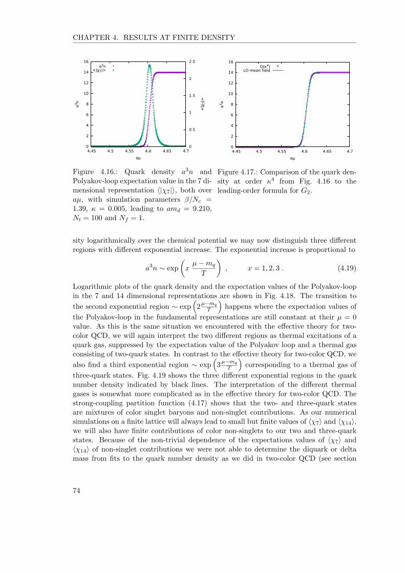
CHAPTER 4. RESULTS AT FINITE DENSITY
0
2
4
6
8
10
12
14
16
4.45 4.5 4.55 4.6 4.65 4.7 0
0.5
1
1.5
2
2.5
a3n
<|χ7|>
aµ
a3n<|χ7|>
Figure 4.16.: Quark density a3n andPolyakov-loop expectation value in the 7 di-mensional representation 〈|χ7|〉, both overaµ, with simulation parameters β/Nc =1.39, κ = 0.005, leading to amd = 9.210,Nt = 100 and Nf = 1.
0
2
4
6
8
10
12
14
16
4.45 4.5 4.55 4.6 4.65 4.7
a3n
aµ
O(κ4)LO mean field
Figure 4.17.: Comparison of the quark den-sity at order κ4 from Fig. 4.16 to theleading-order formula for G2.
sity logarithmically over the chemical potential we may now distinguish three differentregions with different exponential increase. The exponential increase is proportional to
a3n ∼ exp
(xµ−mq
T
), x = 1, 2, 3 . (4.19)
Logarithmic plots of the quark density and the expectation values of the Polyakov-loopin the 7 and 14 dimensional representations are shown in Fig. 4.18. The transition to
the second exponential region ∼ exp(
2µ−mqT
)happens where the expectation values of
the Polyakov-loop in the fundamental representations are still constant at their µ = 0value. As this is the same situation we encountered with the effective theory for two-color QCD, we will again interpret the two different regions as thermal excitations of aquark gas, suppressed by the expectation value of the Polyakov loop and a thermal gasconsisting of two-quark states. In contrast to the effective theory for two-color QCD, we
also find a third exponential region ∼ exp(
3µ−mqT
)corresponding to a thermal gas of
three-quark states. Fig. 4.19 shows the three different exponential regions in the quarknumber density indicated by black lines. The interpretation of the different thermalgases is somewhat more complicated as in the effective theory for two-color QCD. Thestrong-coupling partition function (4.17) shows that the two- and three-quark statesare mixtures of color singlet baryons and non-singlet contributions. As our numericalsimulations on a finite lattice will always lead to small but finite values of 〈χ7〉 and 〈χ14〉,we will also have finite contributions of color non-singlets to our two and three-quarkstates. Because of the non-trivial dependence of the expectations values of 〈χ7〉 and〈χ14〉 of non-singlet contributions we were not able to determine the diquark or deltamass from fits to the quark number density as we did in two-color QCD (see section
74

4.2. Effective Theory for G2 QCD at Finite Density
1x10-12
1x10⁻¹⁰
1x10⁻⁸
1x10⁻⁶
0.0001
0.01
1
100
4.45 4.5 4.55 4.6 4.65 4.7 0.01
0.1
1
10
a3n
<|L
|>
aµ
a3n<|χ7|>
<|χ14|>
Figure 4.18.: Logarithmic plot of the quarkdensity a3n, Polyakov-loop expectationvalue in the 7 dimensional representa-tion 〈|χ7|〉 and 14 dimensional representa-tion 〈|χ14|〉 for the same parameters as inFig. 4.16.
1x10⁻¹⁰
1x10⁻⁸
1x10⁻⁶
0.0001
0.01
1
100
4.45 4.5 4.55 4.6 4.65
a3n
aµ
Figure 4.19.: Logarithmic plot of the quarkdensity a3n, same as in Fig. 4.18. The blacklines indicate different exponential regions,the corresponding slopes are µ, 2µ and 3µ.
4.1.1). We still interpret the main contribution of the two and three-quark states asthermal gases of color singlet diquarks and deltas, as we found a (lightly) bound diquarkin the effective theory of two-color QCD and the G2 strong coupling partition functionalso includes these states as color singlets. Analyzing the partition function one wouldexpect to find also exponential regions corresponding to four and five quark states, evenup to 14 quark states, setting in one after another. However, we are not able to observethese onsets, probably because the saturation of the lattice is suppressing these regions.For the parameter region, where the hopping expansion converges, all the onsets andtransitions we are able to find are analytic. From this, we conclude that to find the phase-transitions to a BEC and the nuclear liquid-gas transition we have to lower temperatures,i.e. larger Nt. To go to sufficiently small temperatures we will have to leave the regionof convergence.
4.2.2. Results outside the Region of Convergence
In the previous sections, the accessible quark masses in the convergence region of thehopping expansion of the effective theory are too large to realize the liquid-gas phasetransition or the transition to a diquark BEC (or respectively, the temperatures are tohigh). On the other hand, one of our main goals is to compare results from the effectivetheory to results from full 4d G2-QCD simulations. Also for reaching that goal we haveto lower the quarks masses to satisfy algorithmic requirements in the full 4d G2-QCDsimulations [99]. We will now increase the hopping parameter to reduce the quark massto compare to results from full 4d simulations. To stay at least close to the region ofconvergence and due to the fact that large temporal extends are numerically not feasible
75

CHAPTER 4. RESULTS AT FINITE DENSITY
2.4 2.45 2.5 2.55 2.6 2.65 2.7
aµ
1/22
1/16
1/12
1/10
1/8
1/Nt
2 4 6 8
10 12
<a3n>
Figure 4.20.: Quark number density overNt and aµ for the parameters β/Nc = 1.4,κ = 0.0357 and Ns = 16. The region of nu-merical instability is marked by the smallirregularity in color.
2.4 2.45 2.5 2.55 2.6 2.65 2.7
aµ
1/22
1/16
1/12
1/10
1/8
1/Nt
2
<|L
|>
Figure 4.21.: Polyakov loop in the 7 dimen-sional representation over Nt and aµ for theparameters β/Nc = 1.4, κ = 0.0357 andNs = 16.
in 4d G2-QCD simulations we can lower Nt. Fig.’s 4.20 and 4.21 show the quark numberdensity a3n and the Polyakov loop in the 7 dimensional representation over Nt and aµfor β/Nc = 1.4, κ = 0.0357 and Ns = 16. The diquark mass for this parameter set isamd = 5.32058. The effective expansion parameter for the chosen parameter set andNt = 24 is κ2Nt/Nc = 0.00437, comparing this to Fig. 4.15 we are just outside out of theconvergence region of the hopping expansion. As a result we find a numerical instabilityfor h ≈ 1 in our data. This numerical instability is a result of the breakdown of theresummation procedure for multiple winding Polyakov loops in the fermion action (seediscussion in sec. 2.4.3). Strictly speaking the instability is there for every parameterset as h → 1, also in the effective theory for two-color QCD. As we are in the regionof convergence of the hopping series we simply do not see the instability because ourresolution in µ is not good enough to approach h = 1 close enough. As we increase theeffective expansion parameter and move outside the region of convergence, the µ rangein which the numerical instability occurs grows larger. Still, outside the instabilityregion we find the expected results: density is almost zero until a3n starts to rise as µapproaches md/2. For even higher chemical potential the density goes into saturation at2Nc = 14. The Polyakov loop also starts to rise from its µ = 0 value as µ→ md/2, takesa maximum at approximately half-filling of the lattice and goes down again for evenlarger µ because of lattice saturation. As Nt grows, we also recognize that density andPolyakov loop are suppressed and the onsets of density and Polyakov loop get sharper,again in agreement with the Silver Blaze property.
76

4.2. Effective Theory for G2 QCD at Finite Density
-2
0
2
4
6
8
10
12
14
2.2 2.3 2.4 2.5 2.6 2.7 2.8
a3n
aµ
eff. TheoryG2 QCD
Figure 4.22.: Comparison of the quark num-ber density from the effective theory andfull G2-QCD simulations.
0
0.5
1
1.5
2
2.5
2.2 2.3 2.4 2.5 2.6 2.7 2.8
<|χ7|>
aµ
eff. TheoryG2 QCD
Figure 4.23.: Comparison of the Polyakovloop expectation value in the 7 dimensionalrepresentation from the effective theory andfull G2-QCD simulations.
Comparison to G2-QCD Results
We will now compare our data from the effective theory to data from full 4d G2-QCDsimulations. In general it is not easy to find parameter sets where the effective theoryand the full theory can be compared. In the derivation of the effective action for the coldand dense regime we neglected all terms subleading in Nt. If we choose Nt too small,this approximation is not valid anymore. On the other hand, large temporal extends ofthe 4d lattice are difficult because they require a lot of computer time. The parameterset we found optimal to compare our data is β/Nc = 1.4, κ = 0.0357 now on a Ns = 8lattice. The temporal extend of the 4d lattice is Nt = 18. With this parameter set wereon the edge of the hopping series’ convergence region. Fig. 4.22 shows a comparisonof the quark number density a3n from the effective theory to full G2-QCD simulations.The errorbars are hidden inside the points. The missing datapoints lie inside the regionof numerical instability. Comparing the results from the effective theory to the resultsfrom the full theory, we see that the agreement is very good up to the region of in-stability. Beyond the region where the effective theory is unstable the effective theoryseems to overestimate the density until it goes into saturation. However, at these valuesof the quark number density we expect lattice artifacts to become important anyway.Also the datapoint from the full theory at aµ = 2.2 seems to deviate from the results ofthe effective theory. Here, the effective theory underestimates the density, predicted byG2-QCD, yet this deviation is not visible on a linear scale. If this deviation at small µ isconnected to the sub-leading terms we neglected in the derivation of the effective theory(see sect. 2.4.6) or due to different behavior of finite size effects is not yet clear and wehave to do more work to figure out which is the case. Fig. 4.23 shows the expectationvalue of the Polyakov loop in the 7 dimensional representation 〈|χ7|〉 from the effectiveand the full theory. We see a good match of the effective theory’s results and the results
77

CHAPTER 4. RESULTS AT FINITE DENSITY
from the full theory up until aµ = 2.6. In the region, where the Polyakov loop dropsdown again due to lattice saturation, we see clear deviations. At small values of thechemical potential the effective theory seems to overestimate the Polyakov loop whencompared to G2-QCD. Again, it is not clear, if this comes from simplifications of theeffective action or if it is a consequence of the theories’ different finite volume behavior.Overall the comparison of the results of the effective theory and full G2-QCD is satisfac-tory, still a lot is to be done on both sides to make reliable conclusions about the rangeof validity of the effective theory and quantitative comparisons. E.g. we would like tohave more datapoints of the effective theory in Fig. 4.22, especially around µ ≈ md/2.Further, we would like to check the effects of different values of β, Nt, κ and Ns on thematching of the results from both theories. Ideally we would like to start deep in theconvergence region of the hopping expansion, with heavy quarks but low temperatureand gradually go to smaller quark masses and/or move closer to the continuum limit.This would take careful choice of the simulation parameters, to make simulations of both,the effective theory and full G2-QCD, feasible and and would require a huge amount ofcomputer time.
4.2.3. On the Nuclear Liquid-Gas Transition and Bose-EinsteinCondensation
In all our simulations of an effective theory for G2-QCD we were not able to observeevidence for Bose-Einstein condensation of diquarks or a nuclear liquid-gas transition.Similar to the effective theory for two-color QCD our quarks are simply much too heavy.One of the main reasons to explore the effective theory outside the hopping expansion’sregion of convergence was to find possible evidence for a phase transition at low temper-atures. The effective theory for QCD does indeed show signs for the nuclear liquid-gastransition, when going outside of the convergence region [84]. We expected to find sim-ilar behavior for the effective theory for G2-QCD, as the nuclear liquid-gas transition isan established feature of G2-QCD [101]. However even for values of κ2Nt/Nc extremelyfar outside the region of convergence we did not find any hints towards a phase transi-tion. One possible reason, why we do not find at least the nuclear liquid-gas transitionis that the additional presence of the thermal diquark gas in G2-QCD somehow coversthe effects of the phase transition as diquark and nucleon onsets are very close to eachother md/2 ≈ m∆/3 in the heavy quark limit and it is difficult to separate between thetwo scales.
78

4.2. Effective Theory for G2 QCD at Finite Density
4.2.4. Results for 2 Dimensional G2-QCD
Since full 4d G2-QCD simulations require a lot of computational resources the Gießengroup, simulating G2-QCD at finite density, now also does simulations in 1+1 dimensionsto reduce computational efforts. Since it is not much work to modify the effective theoryfor 3+1 dimensional space-time to arrive at an effective theory for 1+1 dimensions we willshow the first steps towards comparing the effective theory to a 1+1 dimensional QCD-like theory. One of the main questions of the comparison will be, if one can comparethe theories at all. In the case of a 1+1 dimensional underlying theory, the effectivetheory will be 1 dimensional. Usually one argues that 1 dimensional systems can notundergo a phase transition, this is known as the van Hove theorem [102]. However, thevan Hove theorem is only applicable, if certain requirements are given, one of them beingthe absence of external fields. Since dynamical quarks in the fundamental representationof the gauge group act like external magnetic fields (in the language of spin systems) thevan Hove theorem does not exclude a phase transition in our effective 1d theory. In factthere a plenty of 1d models in the literature that undergo phase transitions [102, 103].What is forbidden, is the Bose-Einstein condensation of diquarks. The Mermin-Wagnertheorem rules out phase transitions connected to th spontaneous breaking of continuoussymmetries in two or less dimensions [104]. The liquid-gas transition is again not affectedby this theorem however, because it is not connected to the spontaneous breakdown ofa continuous symmetry.Now, let us start the discussion with stating the effective action in the case of onedimension. The effective action for the Yang-Mills part is
− Sgeff = uNt∑x
LxLx+1 , (4.20)
the effective coupling λ reduces to its LO expression since in 1+1 dimensions there is noroom for decorations to be attached to the LO diagrams. In the cold and dense regimethe effective action reduces to
− Seff =∑x
log det(1 + hWx)− 2h2
∑x
trhWx
1 + hWxtr
hW~x+1
1 + hW~x+1
+ 2κ4N2
t
N2c
∑x
trhWx
(1 + hWx)2tr
hW~x+1
(1 + hW~x+1)2(4.21)
+κ4N2
t
N2c
∑x
trhWx
(1 + hWx)2
(tr
hWx+1
1 + hWx+1
)2
+ 2κ4N2
t
N2c
∑x
trhWx
(1 + hWx)2tr
hWx−1
1 + hWx−1tr
hWx+1
1 + hWx+1.
Where we also have to adjust the effective coupling
h = (2κeaµ)Nt exp
[2Ntκ
2u
(1− uNt−1
1− u− 4κ2 + 3κ2u
)]. (4.22)
79
CHAPTER 4. RESULTS AT FINITE DENSITY
0
1
2
3
4
5
6
7
8
6.1 6.12 6.14 6.16 6.18 6.2 6.22 6.24
0.2
0.4
0.6
0.8
1
1.2
1.4
1.6
a3n
<|L
|>
aµ
a3n<|L|>
Figure 4.24.: Linear plot of the quark num-ber density and Polyakov loop in the 7 di-mensional representation over aµ for theparameters β/Nc = 1.39, κ = 0.001, Nt =200 and Ns = 32768.
1x10-14
1x10-12
1x10⁻¹⁰
1x10⁻⁸
1x10⁻⁶
0.0001
0.01
1
100
6.1 6.12 6.14 6.16 6.18 6.2 6.22 6.24 0.001
0.01
0.1
1
10
a3n
<|L
|>
aµ
a3n<|L|>
Figure 4.25.: Logarithmic plot of the quarknumber density and Polyakov loop in the 7dimensional representation over aµ for theparameters β/Nc = 1.39, κ = 0.001, Nt =200 and Ns = 32768.
The most important difference to the effective theory for 4 space-time dimensions is themissing power of two in the LO term in eq. (4.21). This is due to the fact that in 1+1dimensions one looses the classification in ’spin up’ and ’spin down’. One importantconsequence becomes visible in the strong coupling partition function
Z(β = 0) =[ ∫
dW (1 + (h+ h6)χ7 + (h2 + h5)(χ7 + χ14)
+ (h3 + h4)(χ27 − χ14) + h7)
]N3s, (4.23)
= [1 + h3 + h4 + h7]N3s .
The partition function of the effective theory does not contain color singlet states, madeup of two-quarks. Fig. 4.24 shows the density and the Polyakov loop in the 7 dimensionalrepresentation from a simulation with the effective action in eq. (4.21) and the parametersβ/Nc = 1.39, κ = 0.001, Nt = 200 and Ns = 32768. The plot looks similar to the 4dcase, hovever the density saturates at Nc = 7 again because we lost the spin degreesof freedom. Fig. 4.25 shows a logarithmic plot of the density and the Polyakov loop inthe 7 dimensional representation for the same parameters as before. In contrast to theresults from the effective theory for 4d G2-QCD we only see two exponential regimes.The slopes in the two regimes are given by µ and 3µ. As predicted by the LO strongcoupling result, we do not find a diquark in the effective theory. First results [99] from1+1d G2-QCD simulations indicate that the theory contains bound diquarks. Howeverthe mass ordering is quite unusual, e.g. the scalar diquark is heavier than the axialvector diquark. This and further evidence seem to indicate that the diquarks consist oftwo quarks with some relative momentum between each other. In the effective theory,two quarks, forming a diquark, have to live on one site or neighboring sites, thus it is
80
4.2. Effective Theory for G2 QCD at Finite Density
not possible for the quarks to carry relative momentum and we do not expect to find thediquarks from the full theory in our effective theory. Retrospectively the absence of anexponential region corresponding to 2µ, though we find color non-singlet two-quark statesin the partition function, is a confirmation of our assumption for the effective theory for4d G2-QCD. Here we made the assumption, that the exponential region corresponding to2µ was mainly there due to color singlet diquarks. Like in the results from the effectivetheory for 4d G2-QCD, the onset of the three quark state happens beyond the pointwhere the Polyakov loop in the seven dimensional representation starts to rise. Nowit is not clear, what relevance the Polyakov loop at finite density has, in connectionwith deconfinement. Yet, if we choose to interpret this thermal three quark state asa thermal gas of fermionic baryons, the rise of the Polyakov loop might be interpretedas a screening effect from the presence of G2-QCD matter in the system rather thandeconfinement. However, the interplay between the onset of baryonic matter, the rise ofthe Polyakov loop and deconfiment at finite density needs more in-depth investigationsthat we are not able to give here.
81

5Summary and Outlook
In this work we have investigated the cold and dense region of the phase diagram oftwo different QCD-like theories: two-color QCD and G2-QCD. In order to perform thisinvestigation we made use of effective theories in terms of Polyakov loops. To calculatethe effective action we have adapted a method, originally developed for QCD. In partic-ular, we determined the effective Polyakov-loop theory by combining a strong couplingand hopping expansion and integrating out spatial gauge degrees of freedom. Using thestrong coupling and hopping expansions in the process, the effective theory is valid forheavy quarks, and away from the continuum limit. However, the advantage of this ef-fective theory is that it is systematically improvable order-by-order and therefore allowsfor a good control over the systematic errors in our approach.We first applied the effective theory to pure SU(2) gauge theory to crosscheck with earlierresults from effective Polyakov-loop theories and full 4d Yang-Mills results. We showedthat our implementation reproduced the known results. Further, we were able to showthat resummations of generalized Polyakov loops in the effective action considerably im-prove the behavior of the local Polyakov loop distribution near the critical temperature.This is an important feature, e.g. for determining the effective Polyakov loop potentialfrom the effective theory.Trying to reproduce the deconfinement phase transition of pure G2 gauge theory in theeffective theory, we saw that resummation of generalized Polyakov loops is not pos-sible in this case. This is due to the fact that the resummation of multiple-windingPolyakov loops does not converge around Tc. We determined the effective coupling con-stant λ(u(β), Nt) up to sixth order in the expansion coefficient of the 7 dimensionalrepresentation u(β). By finding the critical coupling in the effective theory λc and us-ing the analytic relationship between the effective and 4d lattice coupling, we tried todetermine the critical βc. However, by comparing our value of βc to the known valuefor Nt = 6 we found a deviation of about 12%. Including higher orders of u(β) in the
83
CHAPTER 5. SUMMARY AND OUTLOOK
effective coupling turned out to be extremely difficult, as for G2 many group integrals,including plaquettes in different representations, do not vanish but give additional, non-trivial contributions to the effective coupling λ. We therefore tried to include higherorders in u(β) effectively, by fixing λ at one particular Nt to produce the right value forβc. We checked this procedure for SU(2) Yang-Mills theory where it produces reasonableresults, which hence allows us to make predictions for the critical lattice coupling βc forvarious Nt in pure G2 gauge theory as well.We further included dynamical quarks by using the hopping expansion. In the caseof G2-QCD we found the first order deconfinement transition to be stable against theintroduction of heavy quarks. We mapped the G2-QCD phase diagram in the plane ofthe effective couplings λ − h where h is the effective fermion coupling. Decreasing thequark mass, lead to a weakening of the first order phase transition until it ended in a 2ndorder critical point. From the location of the critical point in the λ − h phase diagramwe were able to extract the critical hopping parameter κc. The extracted value turnedout to be too large when compared to 4d G2-QCD simulations, as the extracted κc liesoutside the convergence region of the hopping series.When we applied the effective theory to the cold and dense region of the two-color QCDphase diagram we were able to map out the pseudo-critical line of the deconfinementcrossover at small temperatures. At these low temperatures the Polyakov loop expecta-tion value 〈L〉 stays at its constant zero net-baryon density value, which is dominatedby the finite size of the lattice. Only when we raise the quark chemical potential upto the deconfinement crossover around µpc the Polyakov loop starts to rise. Within theconstant regime of the Polyakov loop we were able to identify a kink in the logarithmicplot of the quark-number density, where the finite temperature behavior of the systemchanges from a Polyakov loop suppressed gas of heavy quarks, existing due to imperfectstatistical confinement, to a thermal gas of free, heavy diquarks. For chemical potentialsabove the quark mass µ > mq the density describes quark matter going into saturationas the lattice gets filled with the maximum number of quarks per site as allowed by thePauli principle.We were able to describe the density of the system by a analytic leading-order formula,with a mean-field description for the Polyakov loop. To describe the Polyakov loopsuppressed quark gas it turned out to be important to use the expectation value of thePolyakov loop 〈L〉, determined from probability distributions of the local Polyakov loop,as mean-field Polyakov loop value. This local Polyakov loop expectation value is abouttwo orders of magnitude smaller than the expectation value of the modulus of its volumeaverage 〈|L|〉, usually used as order parameter in lattice studies. This is due to the fact,that negative values of the local Polyakov loop induce negative local quark numbers.Thus, using the modulus of the volume average overestimates the quark number density.As soon as the expectation value of the Polyakov loop starts to rise, the two quantities〈|L|〉 and 〈L〉 agree with each other. Further, in the regime of the heavy diquark gas(in our simulations the mass of the diquarks was fixed to md = 20 GeV) we saw thatreplacing 2mq by md in the leading-order mean-field formula lead to a near-perfect, pa-rameter free description of the density. Even though our diquarks are only loosely bound2mq − md = 2.8 MeV this replacement made significant difference in the exponential
84

increase of the density. The fact that we are able to describe the density of the systemover the whole range of chemical potentials and temperatures with the mean-field de-scription of the Polyakov loop with only minor adjustments is rather surprising. Themeasured distributions of the local Polyakov loop are not sharply peaked around a meanvalue but are rather broad distributions, suggesting non-negligible fluctuations.We were able to interpret the region between the kink in the logarithmic plot of thedensity and µpc as a thermal gas of heavy diquarks. We found no direct evidence fora Bose-Einstein condensation of those baryonic diquarks, probably because the temper-atures in the range we investigated T > 3.5 MeV are higher than the binding energyof the diquarks. Our diquarks are effectively only held together by confinement, thusthey are not deeply bound dimers in contrast to the usual scenario we find in BECs.Nevertheless, our extrapolation of the diquark onset to T → 0 is in perfect agreementwith µc = md/2 as predicted by chiral perturbation theory. The extrapolation was donefor several values of the lattice coupling β and proofed to be scale independent. Further,we were able to identify a region, where one might be able to find signs of a BEC in thefuture.The phase diagram of cold, dense and heavy G2-QCD also shows a sharp rise of thedensity and the Polyakov loop in the fundamental representations around µ ≈ md/2.For larger µ > md/2 the density goes into saturation at 2 ·Nc = 14. Again we are able todescribe the density by a leading-order mean-field description. However here, we need amean-field description for both fundamental Polyakov loops, in the seven and the four-teen dimensional representation 〈χ7〉 and 〈χ14〉. The expectation value of the Polyakovloops behave similar as in two-color QCD. At small µ the expectation values 〈χ7〉 and〈χ14〉 stay constant at their µ = 0 values until µ ≈ md/2 where they begin to rise. ThePolyakov loop in the seven dimensional representation 〈χ7〉 rises earlier then the one inthe fourteen dimensional representation 〈χ14〉. When we analyze the quark number den-sity in a logarithmic scale, we can again distinguish different exponential regimes. Herewe find three different exponential regimes corresponding to one-, two- and three-quarkstates. The three-quark state corresponds to a fermionic baryon as expected from thegauge invariant spectrum of G2-QCD. By looking at the strong coupling limit of theleading-order partition function we would also expect to find expect to find exponentialregimes corresponding to color singlet states made up of more than three quarks (upto seven quarks). Those exponentials are probably suppressed by the saturation of thelattice.When we applied the effective theory outside the convergence region of the hoppingexpansion we found a small region in µ where we get artifacts in the density and thePolyakov loops caused by numerical instabilities when the chemical potential approachesthe quark mass mq. Outside this instability region we found the expected behavior. Wewere able to compare the results from the effective theory to data from full 4d G2-QCD simulations for one parameter set, on the edge of the convergence region. The4d data matches the results from the effective theory very well for chemical potentialsup to the region where the numerical instabilities set in. Beyond the instability regionand µ > md/2, the data differ slightly until the saturation of the lattice. We are nottoo concerned about those deviations in the data as the region where the deviations
85

CHAPTER 5. SUMMARY AND OUTLOOK
are visible the quark number density has already surpassed the half-filling point of thelattice, thus the density is dominated by lattice artifacts anyway. Unfortunately, wedo not have many datapoints from the full theory to compare our data to, especiallyaround µ ≈ md/2. This makes it e.g. impossible to compare, if the characteristic kinksin the logarithmic plots of the density from the effective theory are also present in thefull theory and, should they appear, if they are at the same locations as in the effectivetheory. In the future, we need more data from full 4d G2-QCD simulations, ideally inthe hopping expansions region of convergence, to compare our data from the effectivetheory to and make robust quantitative comparisons. This lack of 4d data comes fromthe fact that simulating G2-QCD is numerically very expensive, even in the case of fairlyheavy quarks.One way to work around the numerical costs to simulate G2-QCD at finite baryon den-sity might be simulations of dimensionally reduced G2-QCD, in particular the Gießengroup recently started simulations of G2-QCD in 1+1 dimensions. Therefore, we havederived the effective theory for 1+1 dimensional G2-QCD and taken the first steps tomake the comparison to the full theory in the future. In the resulting 1d effective theorywe noticed the absence of color singlet diquarks because the spin degrees of freedomare fundamentally different in 1+1 dimensions. In general, it will be interesting to seeif a 1d effective theory can explain data of a higher dimensional underlying theory, inparticular with regard to a possible first order liquid-gas phase transition.In general we were able to show that effective Polyakov-loop theories for heavy quarks re-flect important physical properties of the underlying QCD-like theories at finite baryondensity and essential differences between the different theories we examined, e.g. thegauge invariant spectrum of the theory or the realization of the Silver Blaze property.We were able to generate lots of results from the effective theories, as numerical simu-lations with the effective actions are rather inexpensive. So far, however, there simplyis not enough data from the full QCD-like theories to compare our results to. Still, wewere able to make a qualitative check of the effective theories and some minor quan-titative comparisons to the existing results from finite density, heavy G2-QCD. Thesecomparisons proved to be satisfying, yet a full-fledged quantitative analysis of the effec-tive theory’s validity was not possible with the few existing results from full QCD-liketheories in the cold and dense regime. More extensive quantitative comparison to theresults of full QCD-like theories and finding the range of validity for the effective theorywill be interesting tasks for future work. This will be possible as soon as results for thefull QCD-like theories with heavy quarks become available.Even though the effective theory seems to realize the Silver Blaze property correctly wehave to take our results with a grain of salt for we were not able to find evidence for anykind of phase transition connected to the onset of baryon density, even when we appliedthe theory at extremely low temperatures beyond the convergence of the hopping series.Maybe our quarks are simply to heavy for the theory to undergo any kind of phasetransition. However, this question will hopefully be answered in the future when higherorders of the combined hopping and strong coupling expansion will be included to pushthe theory closer to the physical pion mass.Another matter is, if the convergence properties of the combined strong coupling and
86

hopping expansion are such that we will be able to apply the effective theory to QCDwith physical pion mass at finite baryon density. This is still under investigation and ifit is possible, it will be a long and difficult way to identify and calculate all terms thathave to be taken into account for reaching physical quark masses. Nevertheless, effectivePolyakov-loop theories still provide valuable understanding about the features of QCD-like theories at finite baryon density on the lattice. This understanding is desirable, asthe more we learn about the phase diagram of QCD-like theories at finite density it turnsout to be challenging to disentangle lattice effects from continuum physics. Of course,this will eventually become important, if we will be able to solve the QCD sign problemin the future.
87

ABasic Facts about Group Representations
In quantum mechanics a transformation is associated with a unitary operator acting onthe Hilbert space.11 Thus, a transformation group of the system is associated with amapping of the group into a set of unitary operators
ρ : G→ U(H) . (A.1)
This means, for every element g of the symmetry group G there is a ρ(g) which isa unitary operator on the Hilbert space H. If the mapping preserves the algebraicstructure, meaning
ρ(g · h) = ρ(g) · ρ(h) ∀g, h ∈ G , (A.2)
we call the mapping ρ a representation of the group G. It will be convenient to think ofrepresentations both as linear operators and as matrices. The connection between themis easy. Take |i〉 to be an orthonormal basis of the Hilbert space. The matrix elementsof the of the linear operator are
(ρ(g))ij = 〈i|ρ(g)|j〉 . (A.3)
Since we are now able to think of representations as matrices we can make two moredefinitions. Two representations ρ and ρ′ are equivalent if they are related by a similaritytransformation
ρ′(g) = Sρ(g)S−1 , (A.4)
for a fixed S and for all g ∈ G. If a representation can be brought into the form
ρ(g) =
(ρ1(g) X(g)
0 ρ2(g)
), (A.5)
11there is also the possibility of anti-unitary operators, but let us ignore them for now.
89

APPENDIX A. BASIC FACTS ABOUT GROUP REPRESENTATIONS
by a similarity tranformation for all g ∈ G it is called reducible. A representation ρ iscalled fully reducible if it is equivalent to a block-diagonal representation ρ′
ρ′(g) = Sρ(g)S−1 =
(ρ′1(g) 0
0 ρ′2(g)
). (A.6)
The Hilbert space H on which ρ acts then breaks down to two orthogonal invariantsubspaces. The representation ρ′ is said to be the direct sum of ρ′1 and ρ′2
ρ′ = ρ′1 ⊕ ρ′2 . (A.7)
A representation is called irreducible, if it is not reducible. For the groups that we willstudy the irreducible representations are all unitary and finite dimensional. The groupswe are studying are Lie groups. Therefore we will not give parameterizations of differentrepresentations but show the group’s generators in the different representations. As areminder, the connection between a given parametrization of a group element and thegenerators of the group is
U(ϕa) = exp[iϕaTa] , (A.8)
where U(ϕa) is the group element, the ϕa are the variables parameterizing the groupand the Ta are the generators of the group. The first example are the generators of thefundamental representation of SU(2), i.e. the smallest dimensional, non-trivial represen-tation of SU(2): The well known Pauli matrices. The generators satisfy the followingcommutation relation
[Ta, Tb] = ifabcTc , (A.9)
where in this case the structure constants fabc are given by two times the totally antisym-metric tensor fabc = 2εabc. If the generators Ta of some representation ρ satisfy (A.9),the matrices −T ∗a satisfy the same relation. Thus they also generate a representation ofthe group, since we have
exp[−iϕaT ∗a ] = U∗(ϕa) . (A.10)
We call this representation the complex conjugate representation of ρ and denote it byρ. The complex conjugate of the fundamental representation is also called the anti-fundamental representation.The generators of a group also satisfy the Jacobi identity
[Ta, [Tb, Tc]] + cyclic permutations = 0 . (A.11)
In terms of the structure constants the above equation becomes
fbcdfade + fabdfcde + fcadfbde = 0 . (A.12)
If we define a new set of matrices (Ta
)bc
= −ifabc , (A.13)
90

A.1. Higher Dimensional Representations
then (A.12) can be rewritten as
[Ta, Tb] = ifabcTc . (A.14)
The representation generated by these matrices is called the adjoint representation. Thedimension of a given representation is equal to the dimension of the Hilbert space itacts on. In case of the adjoint representation the dimension is equal to the number ofgenerators. In the case of SU(2) the dimension of the adjoint representation is three.
A.1. Higher Dimensional Representations
We already saw that the direct sum of two representations ρ1 and ρ2 produces a reduciblerepresentation on the Hilbert space H1⊕H2. There is also the possibility to combine ρ1
and ρ2 via a tensor product
(ρ1 ⊗ ρ2)(g) = ρ1(g)⊗ ρ2(g) . (A.15)
This also gives a representation now acting on the Hilbert space H1 ⊗ H2. The fun-damental theorem on representations of unitary groups states that all irreducible rep-resentations of SU(N) can be generated by tensor products of the fundamental andanti-fundamental representations [105]. In principle one could build all irreducible rep-resentations of SU(N) by calculating tensor products. There is a clever way to workout all these tensor products in a graphical way. This technique to construct all irre-ducible unitary representations for SU(N) relies on so called Young tableaux (For a goodoverview about how to use Young tableaux, see e.g. [105] and [106]).
A.2. Characters Analysis
Similar to ordinary Fourier analysis, we can expand a function depending on groupelements in terms of special functions of the group. Those functions are characteristicfor different representations and are called group characters. The expansion of the gaugeaction in terms of group characters is one particular way to work out the strong couplingexpansion of a gauge theory. Let us start with the definition of the group characters.The character χr of a representation ρr(U) is given by
χr(U) = tr ρr(U) . (A.16)
Its value at unity gives the dimension of the representation
χr(1) = dr . (A.17)
It is a basic but important fact that the trace is independent of the choice of a basis ofour Hilbert space
χr(V UV−1) = χr(U) , U , V ∈ G . (A.18)
91
APPENDIX A. BASIC FACTS ABOUT GROUP REPRESENTATIONS
We say that the character of a representation is a class function and only dependson the invariant angles of a representation. The characters of the irreducible, unitaryrepresentations of a group G are orthogonal∫
dU χr(U)χs(U) = δrs , (A.19)
where χr(U) is the character of the complex conjugate of the representation ρr(U). Fornow, just assume we have a well defined way to integrate over the group manifold,in fact we will define the group integral with the so called Haar measure in the nextsection. Moreover, the theorem of Peter and Weyl states that the characters of theirreducible representations form an orthonormal basis of the Hilbert space of the square-integrable class functions [106]. That means that every square-integrable function on thegroup f(U), obeying f(U) = f(V UV −1) U, V ∈ G can be expanded in terms of groupcharacters
f(U) =∑r∈G
= frχr(U) ,
fr =
∫dU χr(U)f(U) . (A.20)
This is the harmonic analysis on group manifolds and for U(1) we have ordinary Fourieranalysis. The completeness relation of characters is∑
r∈G
χr(U)χr(V ) = δ(UV −1) , (A.21)
where the delta function is defined as∫dU f(U)δ(UV −1) = f(V ) . (A.22)
As an example let us take a look at the action of a single plaquette with Wilson’s gaugeaction
exp[−Sp(Up)] . (A.23)
We write its character expansion in the form
exp[−Sp(Up)] =∑r∈G
drcr(β)χr(Up) , (A.24)
where dr is the dimension of the representation. The explicit coefficients cr(β) are
cr =Ir(β)e−β for U(1),
cr =2
βI2r+1(β)e−β for SU(2). (A.25)
The Ir are modified Bessel functions of the first kind and we encountered these coeffi-cients in the strong coupling expansion of the Yang-Mills action. For the gauge groupSU(3) and other, more complicated gauge groups we are not able to write down theexpansion coefficients in a closed form.
92
A.3. Invariant Integration on Groups
A.3. Invariant Integration on Groups
We will now take a close look at the integration over the group manifold that was alreadyused in the last section. The first ingredient we need for a well defined integrationprocedure is an integration measure. It can be shown that there is a unique, normalizedintegration measure for every compact Lie-group, the Haar measure. It has the follwingproperties ∫
dg =
∫d(gh) =
∫d(hg) =
∫dg−1∫
dg = 1 , (A.26)
where g and h are elements of the group. From this we can read of that the integrationmeasure is in fact invariant under gauge transformations. The Haar measure is com-pletely defined by gauge invariance and normalization for every compact Lie group. Forexample one of the most important features of the Haar measure follows directly fromgauge invariance: ∫
dg f(g) =
∫dg f(hg) . (A.27)
Now we can imediately see that ∫dg g = 0 . (A.28)
An explicit construction of the Haar measure can be obtained as an integral over theparameter space of the group and an according Jacobi determinant (metric tensor) [58].However this construction can be quite tedious for larger groups. We will sketch aprocedure where we do not need the explicit form of the Haar measure. In fact equations(A.26) and (A.28) completely determine all integrals over all possible functions of thegroup elements, since integrals over every product of group elements can be reduced tointegrals over a single group element in some arbitrary representation by Clebsch-Gordandecomposition of the product. The general rule for group integration is
Every integral over an arbitrary function of the group elements is determined by theClebsch-Gordan decomposition of the integrand. If the Clebsch-Gordon decomposition
of the the integrand contains the trivial representation the integral will not vanish.The value of the integral is then given by the multiplicity of the trivial representation.
The general form of an integral emerging in strong coupling or hopping expansions is ofthe form ∫
dg χr1(h1g) · · · · · χri(hig)χrj (hjg−1) · · · · · χrn(hng
−1) (A.29)
where χrl is the character in the representation rl. The general way to compute thisintegral is to calculate the Clebsch-Gordan decomposition of the product in the aboveequation. In particular, if the Clebsch-Gordan decomposition does not contain the trivialrepresentation the integral vanishes, since:∫
dg χr(g) = δr,0 . (A.30)
93
APPENDIX A. BASIC FACTS ABOUT GROUP REPRESENTATIONS
Now we have to find the Clebsch-Gordon decomposition of (A.29). All of the decompo-sition except for terms proportional to the trivial character will vanish. So if the trivialrepresentation is part of the Clebsch-Gordon decomposition then (A.29) will result in asome non-vanishing combination of the hl, where the exact form of the combination isdetermined by the tensor structure of the trivial representation of the decomposition.The simplest example for the integration procedure is:∫
dgχr(gh)χr′(g−1f) = δr,r′
1
drχr(fh) . (A.31)
So in general everything one has to do is work out the Clebsch-Gordon decompositionof (A.29) and determine the tensor structure of the trivial part of the decomposition.Even though this is straight forward and sounds quite simple it takes a lot of effort todo this correctly.
94

BCharacter Expansion for G2
We will now perform the character expansion of the G2 plaquette action. Rememberthat according to eq. (A.24) and eq. (A.25) we can expand the action for a singleplaqutte in the following form
exp[−Sp(U)] =∑r∈G
frχr(U) ,
fr =
∫dUχr(U) exp[−Sp(U)] , (B.1)
where χr(U) is the character in the complex conjugate representation. for our purposesit will be sufficient to take only the first three representations namely the trivial (1) thefundamental (7) and the adjoint (14) representation into account. Since G2 is real wefind that also (7) and (14) are real representations. Therefore we have χ(7) = χ(7) andχ(14) = χ(14). For the trivial representation this is always the case. To carry out theintegration we have to expand the exponential
fr =
∫dUχr(U)
∞∑n=0
1
n!
[β
2Nc(trU + trU †)
]n,
=
∫dU
∞∑n=0
1
n!
[β
Nc
]nχr(U)χn(1,0)(U) , (B.2)
95
APPENDIX B. CHARACTER EXPANSION FOR G2
and find the Clebsch-Gordon decomposition of the character products. The first threeexpansion coefficients up to order β5 read:
f(1) = 1 +β2
2!72+
β3
3!73+ 4
β4
4!74+ 10
β5
5!75,
f(7) =β
7+
β2
2!72+ 4
β3
3!73+ 10
β4
4!74+ 35
β5
5!75,
f(14) =β2
2!72+ 2
β3
3!73+ 9
β4
4!74+ 30
β5
5!75. (B.3)
The results were obtained with the aid of the computer algebra package LiE12. Nowwe compare the expansion coefficients from eq. (2.54) with the coefficients we justcomputed. They are related by
ar =fr
f(1)dr. (B.4)
Therefore we find the expansion parameters
u = a(7) =x
7+x2
14+x3
42− x5
168− x6
36,
v = a(14) =x2
42+x3
42+
5x4
336+
x5
504− 31x6
2016. (B.5)
with x = β7 . We can immediately conclude that if x is such that u is a small parameter
then v is suppressed by another factor of x.
12http://wwwmathlabo.univ-poitiers.fr/∼maavl/LiE/
96
CParametrization of G2 Elements in Terms
of Class-Angles
As G2 is quite a ’large’ group, numerical update algorithms for Monte-Carlo simulationsof G2 are very involved and therefore numerically expensive. Since all the terms in theeffective actions in eqs. (2.141) and (2.155) only depend functions like the trace and thedeterminant of G2 elements we can use a much simpler update algorithm. We alreadysaw in section A.2 that the trace in the fundamental representation is a class functionthat is independent of the choice of a basis:
tr (V UV −1) = trU , U , V ∈ G . (C.1)
This is of cause also true for the determinant:
det(V UV −1) = detU , U , V ∈ G . (C.2)
Since the effective action depends on the Polyakov loops only through class functionswe can evaluate the effective action in an arbitrary basis, moreover we can choose tocalculate every class function in the eigenbasis of its operand. Since all operands inthe effective action (2.155) are of the form (1 + hW ) or hW
(1+hW )n the eigenbasis of theoperands is the eigenbasis of W . The eigenvalues of W are functions of the class anglesonly. Hence, in a Monte-Carlo simulation we have to sample only over the class anglesand not over the whole gauge group. For the case of G2 this simplifies and speeds upour Metropolis algorithm drastically. The eigenvalues of a G2 element in terms of theclass angles can be found by diagonalizing the elements of the maximal torus T of G2.Elements t of T can be parameterized as
t(x, y) = exp[xC5] exp[√
3yC11] , (C.3)
97
APPENDIX C. PARAMETRIZATION OF G2 ELEMENTS IN TERMS OFCLASS-ANGLES
where C5 and C11 are the fifth and eleventh Generator of G2 according to [107]. Thisleads to the following diagonal form of t
t(x, y) =
1
e−i(x−y)
ei(x−y)
e−2iy
e2iy
e−i(x+y)
ei(x−y)
, x, y ∈ [0, π] .
(C.4)When we integrate over class functions it is sufficient to integrate over the class anglesonly, this is done by using the reduced Haar measure. For G2 the reduced Haar measureis given by [95]
dµred =(4χ3(7) − χ
2(7) − 2χ(7) − 10χ(7)χ(14) + 7− 10χ(14) − χ2
(14)) (C.5)
· (7− χ2(7) − 2χ(7) + 4χ(14))dφ1dφ2 (C.6)
Where χ(7) and χ(14) are the characters of the fundamental and the adjoint representationgiven by
χ(7) =1 + 2 cosφ1 + 2 cosφ2 + 2 cos(φ1 + φ2) ,
χ(14) =2(1 + cosφ1 + cos(φ1 − φ2) + cosφ2 + cos(φ1 + φ2)
+ cos(2φ1 + φ2) + cos(φ1 + 2φ2)) .
The angles x, y and φ1, φ2 are related by
x =φ1 − φ2
2, y =
φ1 + φ2
2. (C.7)
And thus the area of integration is φ1, φ2 ∈ [0, 2π].
98
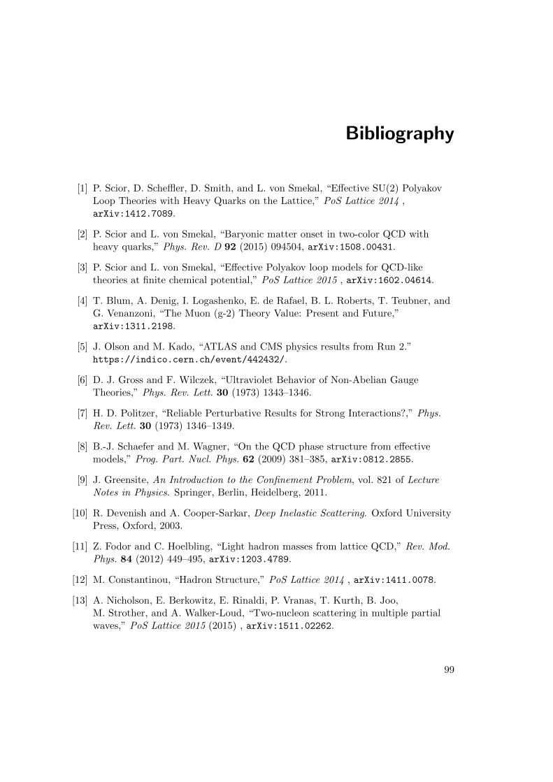
Bibliography
[1] P. Scior, D. Scheffler, D. Smith, and L. von Smekal, “Effective SU(2) PolyakovLoop Theories with Heavy Quarks on the Lattice,” PoS Lattice 2014 ,arXiv:1412.7089.
[2] P. Scior and L. von Smekal, “Baryonic matter onset in two-color QCD withheavy quarks,” Phys. Rev. D 92 (2015) 094504, arXiv:1508.00431.
[3] P. Scior and L. von Smekal, “Effective Polyakov loop models for QCD-liketheories at finite chemical potential,” PoS Lattice 2015 , arXiv:1602.04614.
[4] T. Blum, A. Denig, I. Logashenko, E. de Rafael, B. L. Roberts, T. Teubner, andG. Venanzoni, “The Muon (g-2) Theory Value: Present and Future,”arXiv:1311.2198.
[5] J. Olson and M. Kado, “ATLAS and CMS physics results from Run 2.”https://indico.cern.ch/event/442432/.
[6] D. J. Gross and F. Wilczek, “Ultraviolet Behavior of Non-Abelian GaugeTheories,” Phys. Rev. Lett. 30 (1973) 1343–1346.
[7] H. D. Politzer, “Reliable Perturbative Results for Strong Interactions?,” Phys.Rev. Lett. 30 (1973) 1346–1349.
[8] B.-J. Schaefer and M. Wagner, “On the QCD phase structure from effectivemodels,” Prog. Part. Nucl. Phys. 62 (2009) 381–385, arXiv:0812.2855.
[9] J. Greensite, An Introduction to the Confinement Problem, vol. 821 of LectureNotes in Physics. Springer, Berlin, Heidelberg, 2011.
[10] R. Devenish and A. Cooper-Sarkar, Deep Inelastic Scattering. Oxford UniversityPress, Oxford, 2003.
[11] Z. Fodor and C. Hoelbling, “Light hadron masses from lattice QCD,” Rev. Mod.Phys. 84 (2012) 449–495, arXiv:1203.4789.
[12] M. Constantinou, “Hadron Structure,” PoS Lattice 2014 , arXiv:1411.0078.
[13] A. Nicholson, E. Berkowitz, E. Rinaldi, P. Vranas, T. Kurth, B. Joo,M. Strother, and A. Walker-Loud, “Two-nucleon scattering in multiple partialwaves,” PoS Lattice 2015 (2015) , arXiv:1511.02262.
99
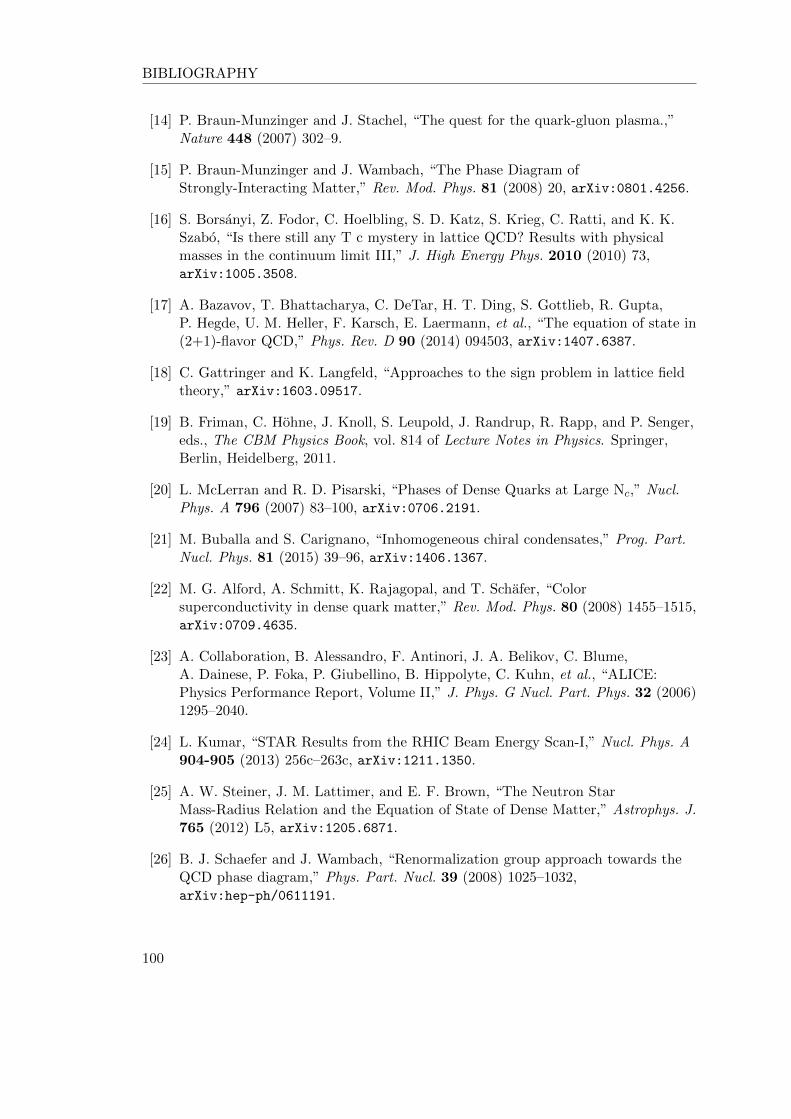
BIBLIOGRAPHY
[14] P. Braun-Munzinger and J. Stachel, “The quest for the quark-gluon plasma.,”Nature 448 (2007) 302–9.
[15] P. Braun-Munzinger and J. Wambach, “The Phase Diagram ofStrongly-Interacting Matter,” Rev. Mod. Phys. 81 (2008) 20, arXiv:0801.4256.
[16] S. Borsanyi, Z. Fodor, C. Hoelbling, S. D. Katz, S. Krieg, C. Ratti, and K. K.Szabo, “Is there still any T c mystery in lattice QCD? Results with physicalmasses in the continuum limit III,” J. High Energy Phys. 2010 (2010) 73,arXiv:1005.3508.
[17] A. Bazavov, T. Bhattacharya, C. DeTar, H. T. Ding, S. Gottlieb, R. Gupta,P. Hegde, U. M. Heller, F. Karsch, E. Laermann, et al., “The equation of state in(2+1)-flavor QCD,” Phys. Rev. D 90 (2014) 094503, arXiv:1407.6387.
[18] C. Gattringer and K. Langfeld, “Approaches to the sign problem in lattice fieldtheory,” arXiv:1603.09517.
[19] B. Friman, C. Hohne, J. Knoll, S. Leupold, J. Randrup, R. Rapp, and P. Senger,eds., The CBM Physics Book, vol. 814 of Lecture Notes in Physics. Springer,Berlin, Heidelberg, 2011.
[20] L. McLerran and R. D. Pisarski, “Phases of Dense Quarks at Large Nc,” Nucl.Phys. A 796 (2007) 83–100, arXiv:0706.2191.
[21] M. Buballa and S. Carignano, “Inhomogeneous chiral condensates,” Prog. Part.Nucl. Phys. 81 (2015) 39–96, arXiv:1406.1367.
[22] M. G. Alford, A. Schmitt, K. Rajagopal, and T. Schafer, “Colorsuperconductivity in dense quark matter,” Rev. Mod. Phys. 80 (2008) 1455–1515,arXiv:0709.4635.
[23] A. Collaboration, B. Alessandro, F. Antinori, J. A. Belikov, C. Blume,A. Dainese, P. Foka, P. Giubellino, B. Hippolyte, C. Kuhn, et al., “ALICE:Physics Performance Report, Volume II,” J. Phys. G Nucl. Part. Phys. 32 (2006)1295–2040.
[24] L. Kumar, “STAR Results from the RHIC Beam Energy Scan-I,” Nucl. Phys. A904-905 (2013) 256c–263c, arXiv:1211.1350.
[25] A. W. Steiner, J. M. Lattimer, and E. F. Brown, “The Neutron StarMass-Radius Relation and the Equation of State of Dense Matter,” Astrophys. J.765 (2012) L5, arXiv:1205.6871.
[26] B. J. Schaefer and J. Wambach, “Renormalization group approach towards theQCD phase diagram,” Phys. Part. Nucl. 39 (2008) 1025–1032,arXiv:hep-ph/0611191.
100

Bibliography
[27] B.-J. Schaefer, J. M. Pawlowski, and J. Wambach, “Phase structure of thePolyakov-quark-meson model,” Phys. Rev. D 76 (2007) 074023,arXiv:0704.3234.
[28] C. Jung, Mesonic Spectral Functions of the Polyakov-Quark-Meson Model.Master’s thesis, TU Darmstadt, 2016.
[29] H. Hansen, W. M. Alberico, A. Beraudo, A. Molinari, M. Nardi, and C. Ratti,“Mesonic correlation functions at finite temperature and density in theNambu–Jona-Lasinio model with a Polyakov loop,” Phys. Rev. D 75 (2007)065004.
[30] C. S. Fischer, J. Luecker, and C. A. Welzbacher, “Locating the critical end pointof QCD,” Nucl. Phys. A 931 (2014) 774–779, arXiv:1410.0124.
[31] G. Eichmann, C. S. Fischer, and C. A. Welzbacher, “Baryon effects on thelocation of QCD’s critical end point,” Phys. Rev. D 93 (2016) 034013,arXiv:1509.0208.
[32] P. de Forcrand and O. Philipsen, “QCD phase diagram for small densities fromsimulations at imaginary µ,” Nucl. Phys. B - Proc. Suppl. 119 (2003) 535–537,arXiv:hep-ph/0301209.
[33] G. Endrodi, Z. Fodor, S. D. Katz, and K. K. Szabo, “The QCD phase diagram atnonzero quark density,” J. High Energy Phys. 2011 (2011) 1, arXiv:1102.1356.
[34] O. Kaczmarek, F. Karsch, E. Laermann, C. Miao, S. Mukherjee, P. Petreczky,C. Schmidt, W. Soeldner, and W. Unger, “The phase boundary for the chiraltransition in (2+1)-flavor QCD at small values of the chemical potential,” Phys.Rev. D 83 (2010) 014504, arXiv:1011.3130.
[35] M. Cristoforetti, F. Di Renzo, G. Eruzzi, A. Mukherjee, C. Schmidt, L. Scorzato,and C. Torrero, “An efficient method to compute the residual phase on aLefschetz thimble,” Phys. Rev. D 89 (2014) 114505, arXiv:1403.5637.
[36] G. Aarts and I.-O. Stamatescu, “Stochastic quantization at finite chemicalpotential,” J. High Energy Phys. 2008 (2008) 018–018, arXiv:0809.5227.
[37] D. Sexty, “Simulating full QCD at nonzero density using the complex Langevinequation,” Phys. Lett. B 729 (2014) 108–111, arXiv:1307.7748.
[38] C. Gattringer, T. Kloiber, and V. Sazonov, “Dual representation for masslessfermions with chemical potential and U(1) gauge fields,” Phys. Rev. D 93 (2015)034505, arXiv:1512.00995.
[39] P. de Forcrand, J. Langelage, O. Philipsen, and W. Unger, “Lattice QCD PhaseDiagram In and Away from the Strong Coupling Limit,” Phys. Rev. Lett. 113(2014) 152002, arXiv:1406.4397 [hep-lat].
101

BIBLIOGRAPHY
[40] M. Fromm, J. Langelage, S. Lottini, M. Neuman, and O. Philipsen, “OnsetTransition to Cold Nuclear Matter from Lattice QCD with Heavy Quarks,” Phys.Rev. Lett. 110 (2013) 122001, arXiv:1207.3005.
[41] M. Fromm, J. Langelage, S. Lottini, and O. Philipsen, “The QCD deconfinementtransition for heavy quarks and all baryon chemical potentials,” J. High EnergyPhys. 2012 (2012) 24, arXiv:1111.4953.
[42] J. Langelage, S. Lottini, and O. Philipsen, “Centre symmetric 3d effective actionsfor thermal SU(N) Yang-Mills from strong coupling series,” J. High Energy Phys.2011 (2011) 57, arXiv:1010.0951.
[43] C. Wozar, T. Kaestner, A. Wipf, and T. Heinzl, “Inverse Monte Carlodetermination of effective lattice models for SU(3) Yang-Mills theory at finitetemperature,” Phys. Rev. D 76 (2007) 085004, arXiv:0704.2570.
[44] J. Greensite and K. Langfeld, “Effective Polyakov line action from strong latticecouplings to the deconfinement transition,” Phys. Rev. D 88 (2013) 074503,arXiv:1305.0048.
[45] J. Engels, J. Fingberg, and M. Weber, “Finite size scaling analysis of SU(2)lattice gauge theory in (3 + 1) dimensions,” Nucl. Phys. B 332 (1990) 737–759.
[46] S. Hands, J. B. Kogut, M.-P. Lombardo, and S. E. Morrison, “Symmetries andspectrum of SU(2) lattice gauge theory at finite chemical potential,” Nucl. Phys.B 558 (1999) 327–346, arXiv:hep-lat/9902034.
[47] S. Hands, S. Kim, and J.-I. Skullerud, “Deconfinement in dense two-color QCD,”Eur. Phys. J. C 48 (2006) 193–206, arXiv:hep-lat/0604004.
[48] S. Cotter, P. Giudice, S. Hands, and J.-I. Skullerud, “Towards the phase diagramof dense two-color matter,” Phys. Rev. D 87 (2013) 034507, arXiv:1210.4496.
[49] T. Boz, S. Cotter, L. Fister, D. Mehta, and J.-I. Skullerud, “Phase transitionsand gluodynamics in 2-colour matter at high density,” Eur. Phys. J. A 49 (2013)11, arXiv:1303.3223.
[50] M. Pepe and U. J. Wiese, “Exceptional Deconfinement in G(2) Gauge Theory,”Nucl. Phys. B 768 (2006) 20, arXiv:hep-lat/0610076.
[51] B. H. Wellegehausen, A. Maas, A. Wipf, and L. von Smekal, “Hadron masses andbaryonic scales in G2-QCD at finite density,” Phys. Rev. D 89 (2014) 056007,arXiv:1312.5579.
[52] F. Karsch and M. Lutgemeier, “Deconfinement and chiral symmetry restorationin an SU(3) gauge theory with adjoint fermions,” Nucl. Phys. B 550 (1999)449–464, arXiv:hep-lat/9812023.
102
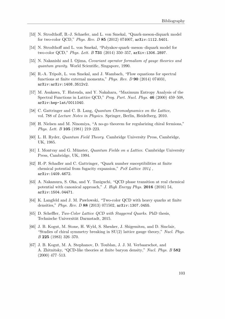
Bibliography
[53] N. Strodthoff, B.-J. Schaefer, and L. von Smekal, “Quark-meson-diquark modelfor two-color QCD,” Phys. Rev. D 85 (2012) 074007, arXiv:1112.5401.
[54] N. Strodthoff and L. von Smekal, “Polyakov-quark–meson–diquark model fortwo-color QCD,” Phys. Lett. B 731 (2014) 350–357, arXiv:1306.2897.
[55] N. Nakanishi and I. Ojima, Covariant operator formalism of gauge theories andquantum gravity. World Scientific, Singapore, 1990.
[56] R.-A. Tripolt, L. von Smekal, and J. Wambach, “Flow equations for spectralfunctions at finite external momenta,” Phys. Rev. D 90 (2014) 074031,arXiv:arXiv:1408.3512v2.
[57] M. Asakawa, T. Hatsuda, and Y. Nakahara, “Maximum Entropy Analysis of theSpectral Functions in Lattice QCD,” Prog. Part. Nucl. Phys. 46 (2000) 459–508,arXiv:hep-lat/0011040.
[58] C. Gattringer and C. B. Lang, Quantum Chromodynamics on the Lattice,vol. 788 of Lecture Notes in Physics. Springer, Berlin, Heidelberg, 2010.
[59] H. Nielsen and M. Ninomiya, “A no-go theorem for regularizing chiral fermions,”Phys. Lett. B 105 (1981) 219–223.
[60] L. H. Ryder, Quantum Field Theory. Cambridge University Press, Cambridge,UK, 1985.
[61] I. Montvay and G. Munster, Quantum Fields on a Lattice. Cambridge UniversityPress, Cambridge, UK, 1994.
[62] H.-P. Schadler and C. Gattringer, “Quark number susceptibilities at finitechemical potential from fugacity expansion,” PoS Lattice 2014 ,arXiv:1409.4672.
[63] A. Nakamura, S. Oka, and Y. Taniguchi, “QCD phase transition at real chemicalpotential with canonical approach,” J. High Energy Phys. 2016 (2016) 54,arXiv:1504.04471.
[64] K. Langfeld and J. M. Pawlowski, “Two-color QCD with heavy quarks at finitedensities,” Phys. Rev. D 88 (2013) 071502, arXiv:1307.0455.
[65] D. Scheffler, Two-Color Lattice QCD with Staggered Quarks. PhD thesis,Technische Universitat Darmstadt, 2015.
[66] J. B. Kogut, M. Stone, H. Wyld, S. Shenker, J. Shigemitsu, and D. Sinclair,“Studies of chiral symmetry breaking in SU(2) lattice gauge theory,” Nucl. Phys.B 225 (1983) 326–370.
[67] J. B. Kogut, M. A. Stephanov, D. Toublan, J. J. M. Verbaarschot, andA. Zhitnitsky, “QCD-like theories at finite baryon density,” Nucl. Phys. B 582(2000) 477–513.
103
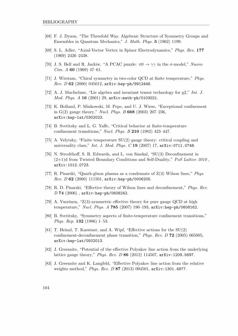
BIBLIOGRAPHY
[68] F. J. Dyson, “The Threefold Way. Algebraic Structure of Symmetry Groups andEnsembles in Quantum Mechanics,” J. Math. Phys. 3 (1962) 1199.
[69] S. L. Adler, “Axial-Vector Vertex in Spinor Electrodynamics,” Phys. Rev. 177(1969) 2426–2438.
[70] J. S. Bell and R. Jackiw, “A PCAC puzzle: π0 → γγ in the σ-model,” NuovoCim. A 60 (1969) 47–61.
[71] J. Wirstam, “Chiral symmetry in two-color QCD at finite temperature,” Phys.Rev. D 62 (2000) 045012, arXiv:hep-ph/9912446.
[72] A. J. Macfarlane, “Lie algebra and invariant tensor technology for g2,” Int. J.Mod. Phys. A 16 (2001) 29, arXiv:math-ph/0103021.
[73] K. Holland, P. Minkowski, M. Pepe, and U. J. Wiese, “Exceptional confinementin G(2) gauge theory,” Nucl. Phys. B 668 (2003) 207–236,arXiv:hep-lat/0302023.
[74] B. Svetitsky and L. G. Yaffe, “Critical behavior at finite-temperatureconfinement transitions,” Nucl. Phys. B 210 (1982) 423–447.
[75] A. Velytsky, “Finite temperature SU(2) gauge theory: critical coupling anduniversality class,” Int. J. Mod. Phys. C 19 (2007) 17, arXiv:0711.0748.
[76] N. Strodthoff, S. R. Edwards, and L. von Smekal, “SU(3) Deconfinement in(2+1)d from Twisted Boundary Conditions and Self-Duality,” PoS Lattice 2010 ,arXiv:1012.0723.
[77] R. Pisarski, “Quark-gluon plasma as a condensate of Z(3) Wilson lines,” Phys.Rev. D 62 (2000) 111501, arXiv:hep-ph/0006205.
[78] R. D. Pisarski, “Effective theory of Wilson lines and deconfinement,” Phys. Rev.D 74 (2006) , arXiv:hep-ph/0608242.
[79] A. Vuorinen, “Z(3)-symmetric effective theory for pure gauge QCD at hightemperature,” Nucl. Phys. A 785 (2007) 190–193, arXiv:hep-ph/0608162.
[80] B. Svetitsky, “Symmetry aspects of finite-temperature confinement transitions,”Phys. Rep. 132 (1986) 1–53.
[81] T. Heinzl, T. Kaestner, and A. Wipf, “Effective actions for the SU(2)confinement-deconfinement phase transition,” Phys. Rev. D 72 (2005) 065005,arXiv:hep-lat/0502013.
[82] J. Greensite, “Potential of the effective Polyakov line action from the underlyinglattice gauge theory,” Phys. Rev. D 86 (2012) 114507, arXiv:1209.5697.
[83] J. Greensite and K. Langfeld, “Effective Polyakov line action from the relativeweights method,” Phys. Rev. D 87 (2013) 094501, arXiv:1301.4977.
104

Bibliography
[84] J. Langelage, M. Neuman, and O. Philipsen, “Heavy dense QCD and nuclearmatter from an effective lattice theory,” J. High Energy Phys. 2014 (2014) 131,arXiv:1403.4162.
[85] G. Munster, “High-temperature expansions for the free energy of vortices and thestring tension in lattice gauge theories,” Nucl. Phys. B 180 (1981) 23–60.
[86] J. Langelage, private communication.
[87] M. Creutz, “On invariant integration over SU(N),” J. Math. Phys. 19 (1978)2043.
[88] J. Langelage and O. Philipsen, “The pressure of strong coupling lattice QCDwith heavy quarks, the hadron resonance gas and the large N limit,” J. HighEnergy Phys. 2010 (2010) 55, arXiv:1002.1507.
[89] N. Kawamoto, “Towards the phase structure of euclidean lattice gauge theorieswith fermions,” Nucl. Phys. B 190 (1981) 617–669.
[90] M. Creutz, “Monte Carlo study of quantized SU(2) gauge theory,” Phys. Rev. D21 (1980) 2308–2315.
[91] P. de Forcrand and L. von Smekal, “’t Hooft Loops, Electric Flux Sectors andConfinement in SU(2) Yang-Mills Theory,” Phys. Rev. D 66 (2001) 011504,arXiv:hep-lat/0107018.
[92] D. Smith, A. Dumitru, R. D. Pisarski, and L. von Smekal, “Effective potentialfor SU(2) Polyakov loops and Wilson loop eigenvalues,” Phys. Rev. D 88 (2013)054020, arXiv:1307.6339.
[93] I. Bogolubsky, V. Mitrjushkin, M. Muller-Preussker, A. Sergeev, and H. Stuben,“Polyakov loops and Binder cumulants in SU(2) theory on large lattices,” Nucl.Phys. B - Proc. Suppl. 129-130 (2004) 611–613.
[94] G. Endrodi, C. Gattringer, and H.-P. Schadler, “Fractality and other propertiesof center domains at finite temperature Part 1: SU(3) lattice gauge theory,”Phys. Rev. D 89 (2014) 054509, arXiv:1401.7228.
[95] B. H. Wellegehausen, A. Wipf, and C. Wozar, “Effective Polyakov loop dynamicsfor finite temperature G 2 gluodynamics,” Phys. Rev. D 80 (2009) 065028,arXiv:0907.1450.
[96] B. H. Wellegehausen, Effektive Polyakov-Loop-Modelle fur SU(N)- und G2-Eichtheorien. Diploma thesis, 2008.
[97] G. Cossu, M. D’Elia, A. Di Giacomo, B. Lucini, and C. Pica, “G 2 gauge theoryat finite temperature,” J. High Energy Phys. 2007 (2007) 100–100,arXiv:0709.0669.
105
BIBLIOGRAPHY
[98] A. Maas, L. von Smekal, B. H. Wellegehausen, and A. Wipf, “Phase diagram of agauge theory with fermionic baryons,” Phys. Rev. D 86 (2012) 111901,arXiv:1203.5653v2.
[99] B. H. Wellegehausen, private communication.
[100] T. D. Cohen, “Functional integrals for QCD at nonzero chemical potential andzero density,” Phys. Rev. Lett. 91 (2003) 222001, arXiv:hep-ph/0307089.
[101] B. H. Wellegehausen and L. von Smekal, “Lattice simulations of G2-QCD atfinite density,” PoS Lattice 2014 , arXiv:1501.06706.
[102] J. A. Cuesta and A. Sanchez, “General non-existence theorem for phasetransitions in one-dimensional systems with short range interactions, andphysical examples of such transitions,” J. Stat. Phys. 115 (2003) 869–893,arXiv:cond-mat/0306354.
[103] C. Herzog, M. Olshanii, and Y. Castin, “A liquid-gas transition for bosons withattractive interaction in one dimension,” Comptes Rendus Phys. 15 (2013)285–296, arXiv:1311.3857.
[104] N. D. Mermin and H. Wagner, “Absence of ferromagnetism orantiferromagnetism in one- or two-dimensional isotropic Heisenberg models,”Phys. Rev. Lett. 17 (1966) 1133–1136.
[105] C. Itzykson and M. Nauenberg, “Unitary Groups: Representations andDecompositions,” Rev. Mod. Phys. 38 (1966) 95–120.
[106] S. Sternberg, Group theory and physics. Cambridge University Press, Cambridge,UK, 1994.
[107] S. L. Cacciatori, B. L. Cerchiai, A. Della Vedova, G. Ortenzi, and A. Scotti,“Euler angles for G2,” J. Math. Phys. 46 (2005) 083512, arXiv:hep-th/0503106.
106
Acknowledgment
First of all I would like to thank Prof. Lorenz von Smekal for giving me the opportunityto do my PhD in his group. In my years as his Master’s and PhD student we had manyinteresting and enlightening discussions, not only about physics. I would like to thankhim for supporting me and especially for not forgetting me and visiting Darmstadt onceper week while the rest of the group moved to Gießen.I am also grateful to Prof. Jochen Wambach for his support in the last years and en-riching discussion during the PhD committees.Next up, I enjoyed working together with my collaborators Sam Edwards, DominikSmith, David Scheffler, Lukas Holicki and Bjorn Wellegehausen - Thank you.I also want to thank all my colleagues from the upper floor as we always had a niceatmosphere and good times unrelated to work. In particular, I would like to mentionChris Jung, Sven Moller, Anton Cyrol for discussion about ’the day, for which we areenvied by the world’, Stefano Carignano for his hatred of the world and people in gen-eral, the ’small’ and the ’tall’ Daniel, Pascal Buscher for supplying me with funny stufffrom the Internet and introducing me to the Japanese cuisine outside of Sushi, MarkusQ. Huber (and also his wife) for organizing countless game sessions at his place, andMarco Schramm for sharing my interest in Scottish Whisky, cooking meat and Eintra-cht Frankfurt.Thank you also to Johannes Weyrich and his girlfriend Linda for numerous sessions onthe ’Lungerbalken’ and keeping me in touch with the world outside of physics.My final thanks go to my girlfriend Michaela and my family for their ongoing support.Without you, I would have never made it this far.
107


Lebenslauf
Name Philipp Friedrich Scior
Geburtstag 9. September 1985
Geburtsort Groß-Umstadt
Staatsangehorigkiet deutsch
Familienstand ledig
2013 - 2016 Promotionsstudium im Fachbereich Physik
an der Technischen Universitat Darmstadt
2009 - 2012 Masterstudium Physik
an der Technischen Universitat Darmstadt
2009 - 2010 Auslandsstudium an der University of Saskatchewan, Saskatoon, Kanada
2006 - 2009 Bachelorstudium Physics
an der Technischen Universitat Darmstadt
2005 - 2006 Freiwilliges Soziales Jahr statt Zivildienst
beim Rettungsdienst des DRK-KV Odenwaldkreis e. V.
2002 - 2005 Schulbesuch am Gymnasium Michelstadt
Abschluss: allgmeine Hochschulreife (Abitur)
109

Erklarung zur Dissertation
Hiermit versichere ich, die vorliegende Dissertation ohne Hilfe Dritter, nur mit denangegebenen Quellen und Hilfsmitteln angefertigt zu haben. Diese Arbeit hat in gle-icher oder ahnlicher Form noch keiner Prufungsbehorde vorgelegen, weiter habe ich nochkeinen Promotionsversuch unternommen.
Darmstadt, den 14.06.2016
Philipp Scior
111