lead and lag compensatorsmaapc/static/files... · a lead compensator increases the bandwidth/speed...

Systems and Control Theory

STADIUS - Center for Dynamical Systems, Signal Processing and Data Analytics

Lead and lag compensators

Lecture 17

1



Overview Definition Lead compensators Impact Design with Bode plots Lag compensators Impact Design with Bode plots Summary of lead and lag compensators Short discussion of lag-lead compensators

2



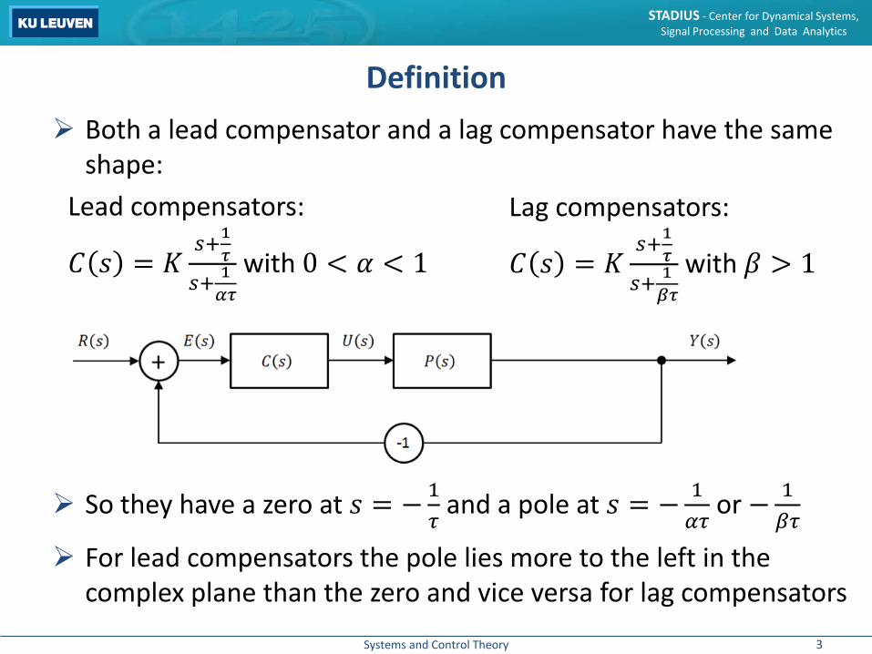
Definition Both a lead compensator and a lag compensator have the same

shape:Lead compensators:

𝐶𝐶 𝑠𝑠 = 𝐾𝐾𝑠𝑠+1𝜏𝜏𝑠𝑠+ 1

𝛼𝛼𝜏𝜏with 0 < 𝛼𝛼 < 1

So they have a zero at 𝑠𝑠 = −1𝜏𝜏

and a pole at 𝑠𝑠 = − 1𝛼𝛼𝜏𝜏

or − 1𝛽𝛽𝜏𝜏

For lead compensators the pole lies more to the left in the complex plane than the zero and vice versa for lag compensators

Lag compensators:


𝛽𝛽𝜏𝜏with 𝛽𝛽 > 1

3



Their differences show themselves clearly by comparing their respective Bode plots:

Definition

Lead compensator Lag compensator

4



Lead compensators

5



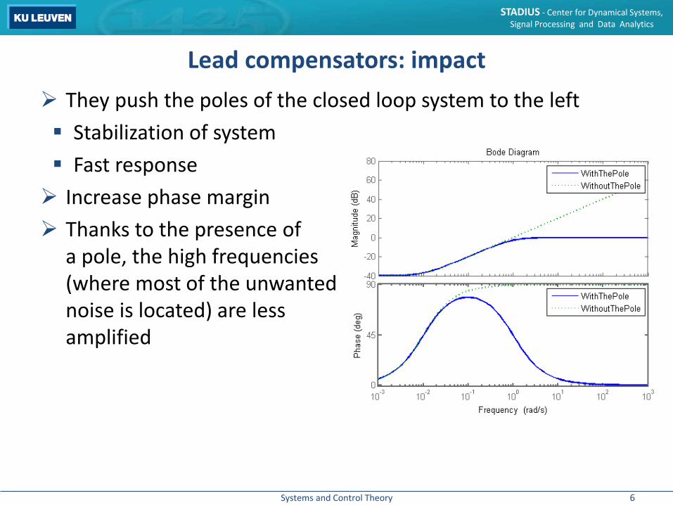
Lead compensators: impact They push the poles of the closed loop system to the left Stabilization of system Fast response Increase phase margin Thanks to the presence of

a pole, the high frequencies (where most of the unwanted noise is located) are less amplified

6



Lead compensators: design with Bode plots Focus: design lead compensators to tune the phase margin

(PM)

0 dB

−180°PM

gain crossover

7



Other design characteristics are also possible

Lead compensators: design with Bode plots

0 dB

−180°

gain margin−3 dB

bandwidth

DC gain

8



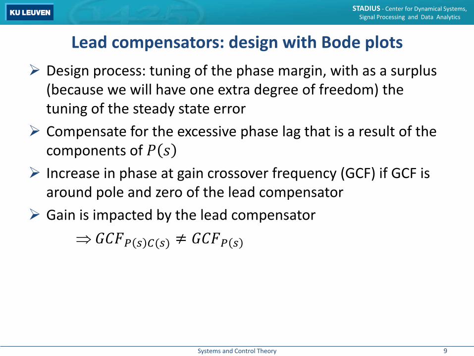
Lead compensators: design with Bode plots Design process: tuning of the phase margin, with as a surplus

(because we will have one extra degree of freedom) the tuning of the steady state error

Compensate for the excessive phase lag that is a result of the components of 𝑃𝑃 𝑠𝑠

Increase in phase at gain crossover frequency (GCF) if GCF is around pole and zero of the lead compensator

Gain is impacted by the lead compensator ⇒ 𝐺𝐺𝐶𝐶𝐺𝐺𝑃𝑃 𝑠𝑠 𝐶𝐶(𝑠𝑠) ≠ 𝐺𝐺𝐶𝐶𝐺𝐺𝑃𝑃 𝑠𝑠

9



Lead compensators: design with Bode plotsHow can we mathematically design a good lead compensator? Required increase in phase gain: 𝜙𝜙 To compensate for increase GCF due to 𝐶𝐶(𝑠𝑠) ⇒ 𝜙𝜙𝑚𝑚 = 𝜙𝜙 + 5°

This will determine 𝛼𝛼 and 𝜏𝜏 𝐾𝐾 will be used to tune the steady state error

Determination of 𝛼𝛼 From the polar plot, we find

sin(𝜙𝜙𝑚𝑚) =12(1−𝛼𝛼)12(1+𝛼𝛼)

= 1−𝛼𝛼1+𝛼𝛼

⇒ 𝛼𝛼 = 1−sin(𝜙𝜙𝑚𝑚)1+sin(𝜙𝜙𝑚𝑚) Polar plot of a lead compensator:

𝛼𝛼(𝑗𝑗𝑗𝑗𝜏𝜏 + 1)/(𝑗𝑗𝑗𝑗𝛼𝛼𝜏𝜏 + 1) where 0 < 𝛼𝛼 < 1

Re

Im

𝑗𝑗 → ∞

12

(1 + 𝛼𝛼)

𝑗𝑗 = 0

0

12

(1 − 𝛼𝛼)

𝑗𝑗𝑚𝑚 𝜙𝜙𝑚𝑚

𝛼𝛼 1

10



Lead compensators: design with Bode plots Determination of τ From the Bode plot of the lead compensator, the maximal

phase is obtained at the frequency of the geometric mean of 1/𝜏𝜏 and 1/𝛼𝛼𝜏𝜏: 𝑗𝑗𝑚𝑚 = 1

𝛼𝛼𝜏𝜏

Use the gain crossover frequency of 𝑃𝑃 𝑠𝑠 𝐶𝐶 𝑠𝑠 as 𝑗𝑗𝑚𝑚:𝑃𝑃 𝑗𝑗𝑗𝑗𝑚𝑚 𝐶𝐶 𝑗𝑗𝑗𝑗𝑚𝑚 = 1

𝑃𝑃 𝑗𝑗𝑗𝑗𝑚𝑚 𝐾𝐾1/𝛼𝛼𝜏𝜏2 + 1/𝜏𝜏2

1/𝛼𝛼𝜏𝜏2 + 1/𝛼𝛼2𝜏𝜏2= 𝑃𝑃 𝑗𝑗𝑗𝑗𝑚𝑚 𝐾𝐾 𝛼𝛼 = 1

20 log 𝑃𝑃 𝑗𝑗𝑗𝑗𝑚𝑚 = −20 log 𝐾𝐾 𝛼𝛼

So the value of 𝑗𝑗𝑚𝑚 can be determined from 𝑃𝑃(𝑠𝑠)’s Bode plot, at least if you know 𝐾𝐾 (our last degree of freedom)

11



Lead compensators: design with Bode plots Determination of 𝐾𝐾 Remember the steady state error for references of the shape 𝐴𝐴𝑡𝑡𝑛𝑛𝜀𝜀 𝑡𝑡 /𝑛𝑛!, with 𝜀𝜀 𝑡𝑡 the step function

We found the error constants 𝐾𝐾𝑝𝑝, 𝐾𝐾𝑣𝑣 and 𝐾𝐾𝑎𝑎 as measures for the steady state error for a proportional (𝑛𝑛 = 0), linear (𝑛𝑛 =1) and accelerating (𝑛𝑛 = 2) reference

So these error constants can be used to find proper values of

𝐾𝐾: lim𝑠𝑠→0

𝐾𝐾𝑠𝑠+1𝜏𝜏𝑠𝑠+ 1

𝛼𝛼𝜏𝜏𝑠𝑠𝑛𝑛𝑃𝑃 𝑠𝑠 = 𝐾𝐾𝛼𝛼 lim

𝑠𝑠→0𝑠𝑠𝑛𝑛𝑃𝑃 𝑠𝑠

12



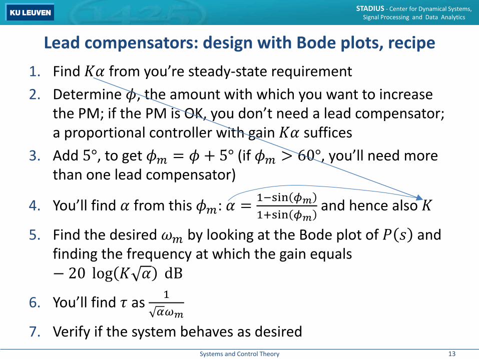
Lead compensators: design with Bode plots, recipe1. Find 𝐾𝐾𝛼𝛼 from you’re steady-state requirement2. Determine 𝜙𝜙, the amount with which you want to increase

the PM; if the PM is OK, you don’t need a lead compensator; a proportional controller with gain 𝐾𝐾𝛼𝛼 suffices

3. Add 5°, to get 𝜙𝜙𝑚𝑚 = 𝜙𝜙 + 5° (if 𝜙𝜙𝑚𝑚 > 60°, you’ll need more than one lead compensator)

4. You’ll find 𝛼𝛼 from this 𝜙𝜙𝑚𝑚: 𝛼𝛼 = 1−sin 𝜙𝜙𝑚𝑚1+sin 𝜙𝜙𝑚𝑚

and hence also 𝐾𝐾

5. Find the desired 𝑗𝑗𝑚𝑚 by looking at the Bode plot of 𝑃𝑃 𝑠𝑠 and finding the frequency at which the gain equals − 20 log 𝐾𝐾 𝛼𝛼 dB

6. You’ll find 𝜏𝜏 as 1𝛼𝛼𝜔𝜔𝑚𝑚

7. Verify if the system behaves as desired13



Lead compensators: design with Bode plots, example Given: system 𝑃𝑃 𝑠𝑠 = 4/𝑠𝑠 𝑠𝑠 + 2 Objective: 𝑃𝑃𝑃𝑃 ≥ 50° and a steady state error for a slope

reference (𝐴𝐴𝑡𝑡𝜀𝜀 𝑡𝑡 ) of maximal 𝐴𝐴/20

14



Lead compensators: design with Bode plots, example1. Steady-state requirement: 𝐾𝐾𝑣𝑣 = 20/𝑠𝑠

lim𝑠𝑠→0

𝑠𝑠𝑃𝑃 𝑠𝑠 𝐶𝐶 𝑠𝑠 = lim𝑠𝑠→0

𝑠𝑠4

𝑠𝑠 𝑠𝑠 + 2𝐾𝐾𝛼𝛼 = 2𝐾𝐾𝛼𝛼 = 20

⇒ 𝐾𝐾𝛼𝛼 = 10

2. Phase margin of 𝐾𝐾𝛼𝛼𝑃𝑃 𝑠𝑠 = 18°⇒ 𝜙𝜙 = 32°

3. 𝜙𝜙𝑚𝑚 = 𝜙𝜙 + 5° = 37°

4. 𝛼𝛼 = 1−sin 𝜙𝜙𝑚𝑚1+sin 𝜙𝜙𝑚𝑚

= 0.24

𝐾𝐾 = 10/𝛼𝛼 = 42PM= 18°

15



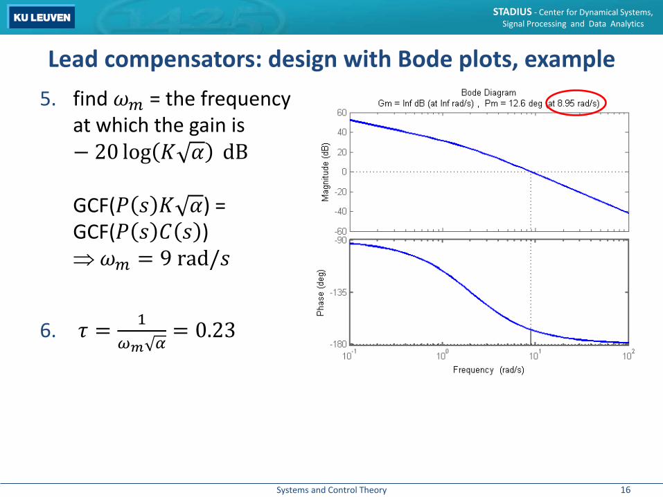
Lead compensators: design with Bode plots, example5. find 𝑗𝑗𝑚𝑚 = the frequency

at which the gain is − 20 log 𝐾𝐾 𝛼𝛼 dB

GCF(𝑃𝑃 𝑠𝑠 𝐾𝐾 𝛼𝛼) = GCF(𝑃𝑃 𝑠𝑠 𝐶𝐶 𝑠𝑠 )⇒ 𝑗𝑗𝑚𝑚 = 9 rad/𝑠𝑠

6. 𝜏𝜏 = 1𝜔𝜔𝑚𝑚 𝛼𝛼

= 0.23

16



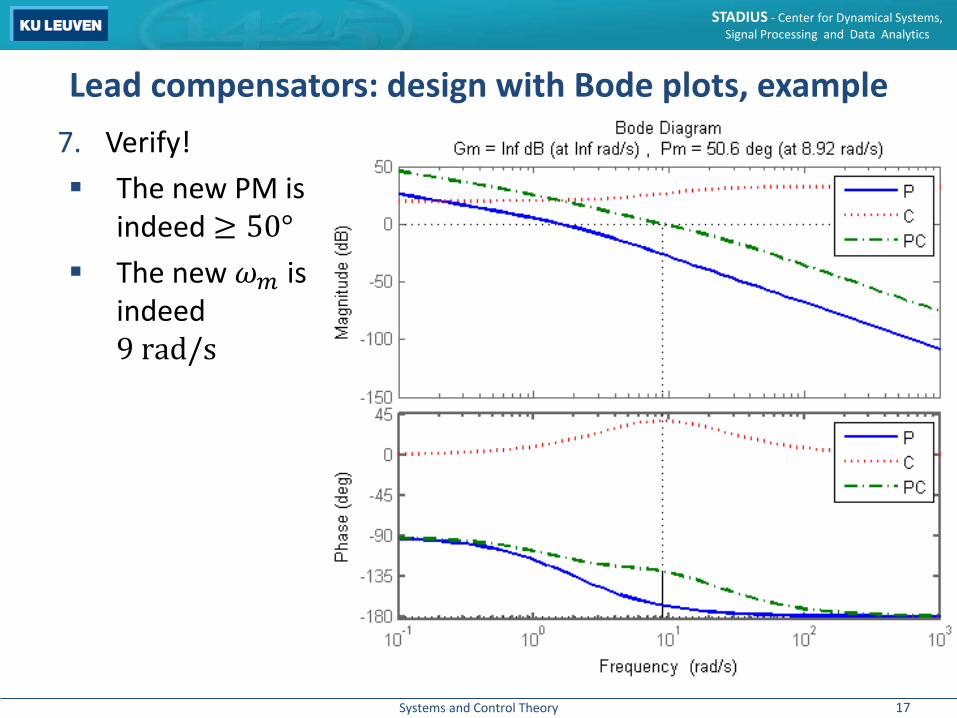
Lead compensators: design with Bode plots, example7. Verify! The new PM is

indeed ≥ 50° The new 𝑗𝑗𝑚𝑚 is

indeed 9 rad/s

17



Lead compensators: design with Bode plots, example Evaluation of impacts of lead compensators: Pushing the poles to the left: this is not directly visible here,

but is linked to the increased BW The increase in bandwidth (this is linked to the response

speed) and the increase in the phase margin were apparent in the Bode plot of 𝑃𝑃 𝑠𝑠 𝐶𝐶 𝑠𝑠

A (small) decrease in the steady-state error occurs, since we designed it as suchWhy small? The steady-state error decreases when the DC gain gets larger, but a lead compensator’s impact on the gain isn’t really built to increase the DC gain, the shape of a lag compensator is much more fit for this

18



Lead compensators: design with root locus Design lead compensators with root locus for time-domain

quantities - use dominant pole locations to fulfill overshoot, rise time, settling time, damping ratio, … requirements

This is not a part of this course For more information, check additional slides on webplatform

19



Lag compensators

20



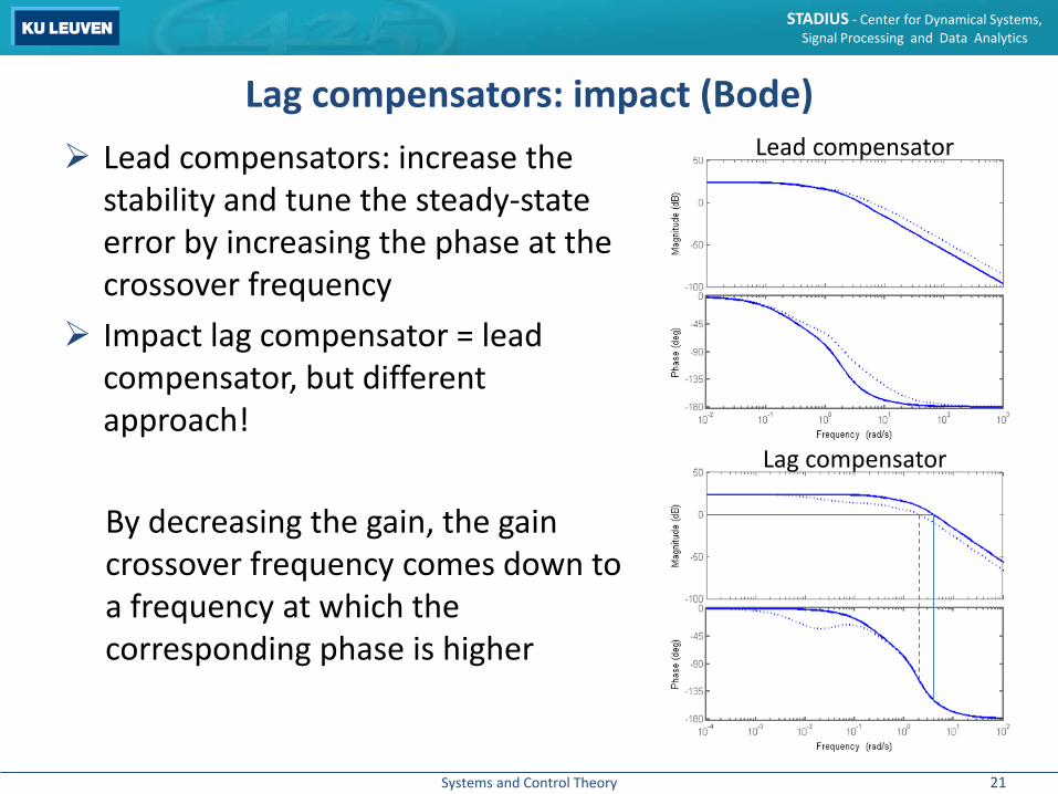
Lag compensators: impact (Bode) Lead compensators: increase the

stability and tune the steady-state error by increasing the phase at the crossover frequency

Impact lag compensator = lead compensator, but different approach!

By decreasing the gain, the gain crossover frequency comes down to a frequency at which the corresponding phase is higher

Lead compensator

Lag compensator

21



Lag compensators: impact (Bode) Large difference between lead and

lag:their effect on the bandwidth of the system and hence on its speed of response

A lead compensator increases the bandwidth/speed of response Good if you want the system to react fast

A lag compensator decreases the bandwidth/speed of response Good if your model is bad at high

frequencies Good to reduce the impact of (mostly

high-frequency) noise

3 dB

Lead compensator

3 dB

Lag compensator

22



Lag compensators: design with Bode plots


𝛽𝛽𝜏𝜏with 𝛽𝛽 > 1

Design process: we use one degree of freedom to

have a sufficient drop in gain one degree of freedom to

push the drop in the phase to lower frequencies (that way we can use ∠ 𝑃𝑃 𝑠𝑠 as an approximation of ∠ 𝑃𝑃 𝑠𝑠 𝐶𝐶 𝑠𝑠 reliably to some extent

one more degree of freedom to tune the steady state error

23



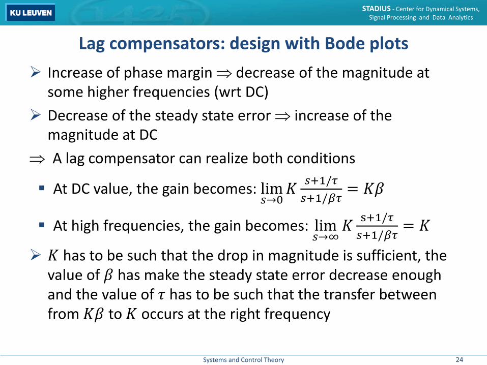
Lag compensators: design with Bode plots Increase of phase margin ⇒ decrease of the magnitude at

some higher frequencies (wrt DC) Decrease of the steady state error ⇒ increase of the

magnitude at DC⇒ A lag compensator can realize both conditions

At DC value, the gain becomes: lim𝑠𝑠→0

𝐾𝐾 𝑠𝑠+1/𝜏𝜏𝑠𝑠+1/𝛽𝛽𝜏𝜏

= 𝐾𝐾𝛽𝛽

At high frequencies, the gain becomes: lim𝑠𝑠→∞

𝐾𝐾 s+1/𝜏𝜏𝑠𝑠+1/𝛽𝛽𝜏𝜏

= 𝐾𝐾

𝐾𝐾 has to be such that the drop in magnitude is sufficient, the value of 𝛽𝛽 has make the steady state error decrease enough and the value of 𝜏𝜏 has to be such that the transfer between from 𝐾𝐾𝛽𝛽 to 𝐾𝐾 occurs at the right frequency

24



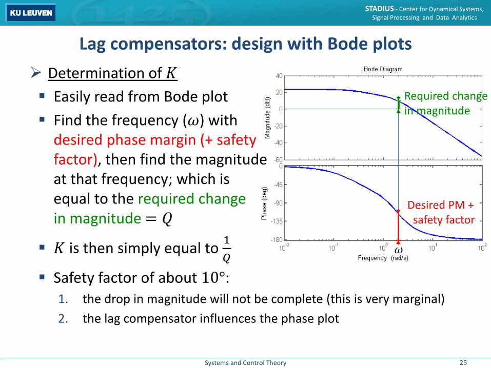
Lag compensators: design with Bode plots Determination of 𝐾𝐾 Easily read from Bode plot Find the frequency (𝑗𝑗) with

desired phase margin (+ safety factor), then find the magnitudeat that frequency; which is equal to the required changein magnitude = 𝑄𝑄

𝐾𝐾 is then simply equal to 1𝑄𝑄

Safety factor of about 10°:1. the drop in magnitude will not be complete (this is very marginal)2. the lag compensator influences the phase plot

Desired PM + safety factor

Required change in magnitude

𝑗𝑗

25



Lag compensators: design with Bode plots Determination of 𝛽𝛽 We can find 𝐾𝐾𝛽𝛽 in a similar way as we found 𝐾𝐾𝛼𝛼 for lead

compensators Translate steady state error requirement in a requirement on 𝐾𝐾𝑝𝑝 (= lim

𝑠𝑠→0𝑃𝑃 𝑠𝑠 𝐶𝐶 𝑠𝑠 ), 𝐾𝐾𝑣𝑣 (= lim

𝑠𝑠→0𝑠𝑠𝑃𝑃 𝑠𝑠 𝐶𝐶 𝑠𝑠 ), 𝐾𝐾𝑎𝑎 (=

lim𝑠𝑠→0

𝑠𝑠2𝑃𝑃 𝑠𝑠 𝐶𝐶 𝑠𝑠 ), or another error constant With this 𝐾𝐾𝑝𝑝/𝑣𝑣/𝑎𝑎/... and lim

𝑠𝑠→0𝑃𝑃 𝑠𝑠 we can determine

lim𝑠𝑠→0

𝐶𝐶 𝑠𝑠 = 𝐾𝐾𝛽𝛽

26



Lag compensators: design with Bode plots Determination of 𝜏𝜏 Take 𝜏𝜏 large enough such that the

magnitude is almost entirely dropped, and the phase drop has almost disappeared

Take the zero one decade smaller than the frequency (𝑗𝑗) at which𝑃𝑃 𝑠𝑠 had the desired phase (−180° + the desired phase margin + a safety factor of 10°)

Verify the effect of a single zero at a frequency one decade smaller than 𝑗𝑗

• The drop in magnitude is as good as complete• The drop in phase cannot be more than −5.7°

27



Lag compensators: design with Bode plots Let’s translate all of this into a recipe again:1. Translate your steady-state requirement into a requirement

on lim𝑠𝑠→0

𝐶𝐶 𝑠𝑠 = 𝐾𝐾𝛽𝛽 and verify whether a proportional controller with gain 𝐾𝐾𝛽𝛽 would suffice

2. Read 𝑗𝑗, the frequency at which the phase margin equals −180° + your desired phase margin + 10°, off the Bode diagram; this allows us to compute 𝜏𝜏 = 10/𝑗𝑗

3. Read 𝑄𝑄, the magnitude at 𝑗𝑗 off the Bode plot and determine 𝐾𝐾 = 1/𝑄𝑄

4. Determine 𝛽𝛽 = 𝐾𝐾𝛽𝛽/𝐾𝐾5. Verify the behavior of the resulting system

28



Lag compensators: design with Bode plots, example

Given: system 𝑃𝑃 𝑠𝑠 = 1𝑠𝑠 𝑠𝑠+1 𝑠𝑠+2

Objective: 𝑃𝑃𝑃𝑃 ≥ 40° and a ramp input (𝐴𝐴𝜀𝜀 𝑡𝑡 ) results in a steady state error of at most 𝐴𝐴/5, or 𝐾𝐾𝑣𝑣 = 5/𝑠𝑠

29



Lag compensators: design with Bode plots, example1. Steady-state requirement 𝐾𝐾𝑣𝑣 = 5/𝑠𝑠

lim𝑠𝑠→0

𝑠𝑠𝐶𝐶 𝑠𝑠 𝑃𝑃 𝑠𝑠 = 12

lim𝑠𝑠→0

𝐶𝐶 𝑠𝑠 = 5 /𝑠𝑠

⇒ 𝐾𝐾𝛽𝛽 = 10

2. Look at the effect of𝐾𝐾𝛽𝛽𝑃𝑃 𝑠𝑠 on the Bode plot

3. Adding a gain of 10 = 20 dB to get the right steady state error, the phase gain would become negative which means the system would become unstable

4. ⇒ Lag compensator is necessary30



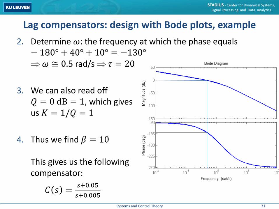
Lag compensators: design with Bode plots, example2. Determine 𝑗𝑗: the frequency at which the phase equals

− 180° + 40° + 10° = −130°⇒ 𝑗𝑗 ≅ 0.5 rad/s ⇒ 𝜏𝜏 = 20

3. We can also read off 𝑄𝑄 = 0 dB = 1, which gives us 𝐾𝐾 = 1/𝑄𝑄 = 1

4. Thus we find 𝛽𝛽 = 10

This gives us the followingcompensator:

𝐶𝐶 𝑠𝑠 = 𝑠𝑠+0.05𝑠𝑠+0.005

31



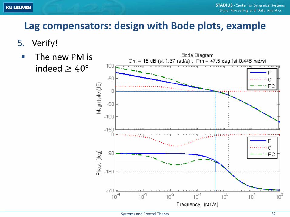
Lag compensators: design with Bode plots, example5. Verify! The new PM is

indeed ≥ 40°

32



Lag compensators: design with Bode plots, exampleGoal of lag compensator? To decrease the magnitude in order to shift the gain crossover

frequency to a frequency with a larger phase margin; the extra degree of freedom is then used to tune the steady-state error

In this example: lag compensator to tune the steady state error with a minimal impact on the phase margin

So this time we used a lag compensator to increase the DC gain but leave the gain at higher frequencies unaltered

33



Lag compensators: impact (root locus) We can also use lag compensators to reduce the steady state

error significantly but with a marginal impact on (the relevant part of) the root locus

On top of that, we still have one degree of freedom that allows us to pick any position on that root locus!

This is useful if the desired closed loop poles are already on the root locus, but if a proportional controller would give a too large steady-state error

We will not go further into detail in design of lag compensators using root locus

For more information, check additional slides on webplatform

34



Summary

35



Summary of lead and lag compensators

Lead compensator Lag compensatorBode plot design

• Increasing the stability margins

• Tuning the steady state error• Relative increase in the high

frequency gain (good if you want a faster response)

• Increasing the stability margins

• Tuning the steady state error• Relative decrease in the high

frequency gain (good if your model behaves bad at high frequencies which is fairly common, as noise tends to be dominant at high frequencies)

Root locus design

• Changing the shape of the root locus for a faster response

• Decreasing the steady state error without changing the shape of the root locus

36



Summary of lead and lag compensators Another important thing to note is that we ‘use’ different

aspects for the design of lead and lag compensators: When we design lead compensators we make use of the fact

that it can add some phase at a specific frequency When we design lag compensators we make use of the fact

that it permits to add gain at low frequencies (which improves the steady-state error), and a reduction of the gain at high frequencies (which reduces instability of the closed loop system)

37



Lag-lead compensators

38



Short discussion of lag-lead compensators In some cases you would want to combine the effects of a lag

and a lead compensator: Frequency domain:

In most cases a lead compensator is more fit to increase the phase margin and a lag compensator is better at decreasing the steady-state error

Time domainYou might want to adapt the root locus with a lead compensator, and decrease the steady-state error while leaving the new root locus unaltered with a lag compensator

39



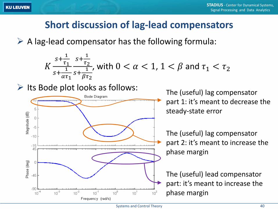
Short discussion of lag-lead compensators A lag-lead compensator has the following formula:

𝐾𝐾𝑠𝑠+ 1

𝜏𝜏1𝑠𝑠+ 1

𝛼𝛼𝜏𝜏1

𝑠𝑠+ 1𝜏𝜏2

𝑠𝑠+ 1𝛽𝛽𝜏𝜏2

, with 0 < 𝛼𝛼 < 1, 1 < 𝛽𝛽 and 𝜏𝜏1 < 𝜏𝜏2

Its Bode plot looks as follows: The (useful) lag compensator part 1: it’s meant to decrease the steady-state error

The (useful) lag compensator part 2: it’s meant to increase the phase margin

The (useful) lead compensator part: it’s meant to increase the phase margin

40



Short discussion of lag-lead compensators The disadvantage of a lag-lead compensator over a lag

compensator or a lead compensator is its increased complexity, and hence cost (the same way a lag or lead compensator is more complex/costly than a proportional controller)

We will not go over a design procedure for this other typical classical control component, as it does not add more insight than the separate compensators do

41

lead and lag compensatorsmaapc/static/files... · a lead compensator increases the bandwidth/speed...

Documents