leaf diffusion resistance to water vapour and its …

581.116.1.037.8:581-45 633.15:58

MEDEDELINGEN LANDBOUWHOGESCHOOL WAGENINGEN • NEDERLAND • 74-21 (1974)

LEAF DIFFUSION RESISTANCE TO WATER VAPOUR AND ITS DIRECT MEASUREMENT

III. RESULTS R E G A R D I N G THE IMPROVED D IFFUSION POROMETER IN GROWTH ROOMS

AND FIELDS OF INDIAN CORN (ZEA MAYS)

C. J. STIGTER, B. LAMMERS

Laboratory of Physics and Meteorology, Agricultural University, Wageningen, The Netherlands

(Received 17-IX-1974)

H. VEENMAN & ZONEN B.V. - WAGENINGEN - 1974

'o!A(0((: i

TABLE OF CONTENTS

1. INTRODUCTION 1

2 . CALIBRATION OF DUMMY RESISTANCES 3 2.1. Calculations of membrane resistances 3 2.2. Measurements of membrane resistances 5

3. PROBLEMS WITH MEASUREMENTS ON LEAVES 9 3.1. Classification 9 3.2. Temperature measurements on leaves 9 3.3. Influences of the device 14 3.4. The quotient of long and short transient times 15

4. FIELD MEASUREMENTS IN INDIAN CORN 18 4.1. General remarks 18 4.2. Temperature measurements 18 4.3. Changes in the opening status of the stomata 20 4.4. Resistance profiles within a crop stand 29

5. SUMMARY 48

6. ACKNOWLEDGEMENTS 50

7. REFERENCES 51

8. APPENDIX 1.

Data of the porous membranes used 54

9. APPENDDC 2. A mathematical approximation for the diffusion resistance of membranes with holes having circular axial cross section 57

10. APPENDIX 3. An improved method for determining diffusion resistance of porous membranes by simple evaporation experiments 60

11. APPENDIX 4. A check on influences of the temperature measuring system in growth chamber experiments on leaves 69

12. APPENDIX 5. A cause for deviations from the theoretically expected ratio of long and short transient times 72

13. APPENDIX 5.

A guide to users of porometers 75

1. I N T R O D U C T I O N

In search of an accurate method for measuring directly leaf diffusional resistance profiles inside crop canopies, we found a few years ago from the existing literature at that time that no method was sufficiently developed to rely on without further research. It became clear from an earlier published review (STIGTER,

1972; this paper will be refered to further on as (I)) that diffusion porometers were most promising to yield quantitatively accurate results. Especially the leaf diffusion resistance meter of the type originally developed by Wallihan and Van Bavel seemed to be in principle a suitable apparatus for field measurements.

In the literature till 1970 already several modifications of this device were reported (Comp. (I), Table 2). It became clear, however, from reports in the literature on more intensified field and laboratory use of the instrument, that the accuracy of the types constructed (and calibrated) so far was lower than originally expected (Comp. STIGTER et al., 1973; this paper will be refered to further on as (II)). Preliminary investigations with a prototype built for use in our Indian corn project (I) contributed sensibly to underline this more pessimistic view point. Therefore we decided to investigate the prototype mentioned more thoroughly.

Results of this research were already reported in detail (II). A summary was given recently (STIGTER, 1974). We were able to develop an improved leaf diffusional resistance meter which can be soundly calibrated. Especially the unpredictable changes in properties of the used humidity sensors were taken into consideration, for which a proper measuring strategy was adopted.

Examples of such calibrations were given in (II). We reported there and in (I) that the only reliable calibration methods are based on the use of dummy epidermal resistances in the form of metal multipore membranes. The independent determination of the resistance values of such membranes, by evaporation experiments in the growth room and by calculations, is reported in this final publication of the series. We also used the dummy epidermal resistances to show that the field measuring strategy is correct.

We still have to deal with problems encountered in the measurements on leaves, especially in relation to the temperature of the measured leaf parts. Referring to what has been said on internal leaf processes in (I) we will indicate that the apparatus is not influencing to any measurable extend the original diffusion processes within the leaf and through the epidermis. Regarding the epidermis this holds as long as the state of opening of the stomata remains unaffected. This constant resistance of the stomata during the measurement can be accurately checked with our measuring method.

Further we will report on measurements on artificial leaves and bean leaves in the growth chamber. By these measurements we showed the validity of the temperature measuring system. Finally measurements in Indian corn will be reported. The problems of obtaining canopy profiles are in first instance sample

Meded. Landbouwhogeschool Wageningen 74-21 (1974) 1

problems (MONTEITH, 1973). The factors involved and the results obtained will form the closing part of this study.

Meded. Landbouwhogeschool Wageningen 74-21 (1974)

2. C A L I B R A T I O N OF D U M M Y RESISTANCES

2.1. CALCULATIONS OF MEMBRANE RESISTANCES.

Formulae for the calculation of vapour diffusional resistance of single cylindrical pores (or per unit surface of multiporous membranes made up of cylindrical holes) are well known from diffusion theory (e.g. PENMAN and SCHO-

FIELD, 1951; LEE and GATES, 1964; LEE, 1967; MEIDNER and MANSFIELD, 1968;

MONTEITH, 1973). For a porous membrane made up of n cylindrical pores of length i and diameter d, per unit of surface, the resistance, Rm, is normally taken to be:

41 1 R" = M ) + 2X2dnD- ( 1 )

In (1) the diffusion coefficient D is a temperature dependent variable (I, p. 22, 23). The first term of (1) is the diffusion resistance of the tubes proper. The second term is the expression for the diffusional end effects (or 'end-corrections' as PENMAN and SCHOFIELD (1951) called them after an analogous effect for organ pipes) at both sides of the membrane (I, Ch. 3). It represents the diffusion resistance of a semi-infinite half space, completely insulated at the free surface with the exception of n independent spots of given constant and uniform concentration (see e.g. CARSLAW and JAEGER, 1959, Ch. VIII, 8.2.1, p. 215 ; GRIGULL,

1963,p. 111). It is important to note here that in expressions for the calculation of the

epidermal resistance of real leaves, some authors assume a large distance from the lower side of stomatal tubes to the cell walls lining the stomatal cavity (e.g. PARLANGE and WAGGONER, 1970). Consequently (1) may be used in such calculations. Others (e.g. MONTEITH, 1973) believe that the internal end effect is lower than the end effect at the outer leaf side and often even negligible (Comp. I, p. 17). In the latter case the second term of (1) reads for cylindrical pores IßdnD.

In obtaining (1), the resistance of one pore is divided by n, the number of holes per unit of surface, and the end effects are taken to be mutually independent. As outlined in (I, p. 18), this was proved by PARLANGE and WAGGONER

(1970) to be correct for interstomatal distances occurring in nature. They derived mathematically that the use of (1) for pores with straight walls is valid as long as interstomatal distance, i, is at least three times the (maximum) stomatal width d. Our membrane holes (and also real stomates) differ considerably from this straight wall pore type since they are more or less funnel-shaped (see Fig. 1 ; all characteristics may be found summarized in Appendix 1). For the narrowest (throat) end of the holes in our membranes (d = d„ Fig. 1) the PARLANGE and WAGGONER condition is fully satisfied. At the mouth (d = dm) of the holes, however, the situation differs too much from the straight wall situation to apply this condition.


FIG. 1. Vertical cross section through the centre of holes in the porous membranes. We have denned the following parameters: i = 'interstomatal' distance; d, = hole diameter at the throat; dm = hole diameter at the mouth; / = thickness of the membrane; ƒ = flat part between two holes at the mouth side. The walls are circular shaped in vertical cross section.

PENMAN and SCHOFIELD (1951) considered the same problem for stomates with hyperbolic axial cross section. They finally recommended that the effective radius of stomatal pores 'as a working rule until experience indicates the need for improvement' should be taken as

d' = ^dt Vdtdm

and that the end effect at the mouth end should be taken

R 1

end, 1 Id'nD

(2)

(3)

Now the ratio between i and d' is for almost all the membranes we used higher than three, except for 15 S, 30 R and 125 P (Table App. 1.1) where it is between 2.5 and 3. We feel, therefore, that if d' is a good choice for the effective diameter in our case, the best approximation for all membranes is found using (1) in the following form :

Rm — Rpc

4£

+

Rend,

1

1 + Rend, 2 —

1 Tz(d')2nD Id'nD 2dtnD

(4)

The proof that PENMAN and SCHOFIELDS' more or less intuitive choice for d' (2) is valid for our holes is given in Appendix 2.

As the manufacturer indicates (VECO Zeefplatenfabriek, Eerbeek, private communication), our membranes have holes from which each vertical cross section is bounded by almost circular curves (Fig. 1). This makes it possible to compare the values forecasted by the first term of (4) with a mathematically more sound approximation. As shown in Appendix 2 the choice in (2) is excel-


TABLE 1. Comparison of calculated diffusion resistances in s/cm by PENMAN/SCHOFIELDS' approximation and measured resistances by evaporation experiments and via intercomparison using the diffusion porometer of nickel membranes with funnel shaped holes (Fig. 1 and Appendix 1).

Membrane type

20 W 20 T VERO 15 T 20 T 15 S 30 T 40 T 30 R

100 T 80 T

125 T \ 100 R 125 R 125 P )

Measured resistance (evaporation exp.)

10.00 ± 0.20 5.80 ± 0.10 5.50 ± 0.15 4.95 ± 0.10 2.75 ± 0.25 2.70 ± 0.20 2.30 ± 0.15 1.40 ± 0.15 0.80 ± 0.15 0.55 ±0.15

Reference membranes

Measured resistance (diffusion porometer)

9.5 ±0 .3 5.70 ± 0.10 5.45 ± 0.10 4.65 ± 0.20 2.75 ± 0.10 2.75 ± 0.10 2.25 ± 0.10 1.50 ± 0.10 0.90 ± 0.05 0.65 ± 0.05 0.55 ± 0.05 0.45 ± 0.05 0.35 ± 0.05 0.35 ± 0.05

Calculated resistance (PENMAN/SCHOFIELD)

9.4 ±0 .6 6.10 ± 0.35 5.55 ± 0.25 4.85 ± 0.25 2.60 ± 0.10 2.75 ± 0.10 2.05 ± 0.10 1.35 ±0.10 1.00 ± 0.05 0.65 ± 0.02 0.50 ± 0.02 0.38 ± 0.02 0.36 ± 0.02 0.28 ± 0.02

lent for our case with an approximately circular shape of the cross section (Fig. 1, see also Appendix 1 for this approximation) using:

d, + 2£ (5)

Table 1 (third column) shows the results of the calculations using equation (4). Accuracy limits have been calculated from the accuracy of our own microscope measurements, over the complete membrane, ofi, d, and n, as indicated in Appendix 1.

2.2. MEASUREMENTS OF MEMBRANE RESISTANCES.

Since most calibration methods in use were not very accurate in practice (II, p. 15 and 16), and because of the need for reliable research on the behaviour of the sensor (II, Ch. 6.4), it appeared to be dangerous to rely on the PENMAN/

SCHOFIELD formulae without further checking. Therefore we tried to measure as accurately as possible the diffusion resis

tances of our membranes. This can be done in principle by relatively simple evaporation experiments. Such experiments ask for accurate environmental control and some reasoning on physical transport processes within and over receptacles sealed with the nickel membranes (Fig. 2). The experiments are described in detail, with their theoretical background, in Appendix 3. The results given there are summarized in the first column of Table 1. Comparing these measured values in the first column with the calculated ones in the third column, we see


FIG. 2. Receptacles, of two different types, used for evaporation experiments. The receptacles are sealed with porous membranes which are, detached from the receptacles, used as dummy epidermal diffusion resistances for calibration of the porometer. For details see Fig. App. 3.1.

that error limits overlap or touch each other in all cases. In the experiments with the leaf diffusion meter, reported in (II), we used

membranes disjointed from the receptacles without thermocouple (Appendix 3). Therefore we used the values of the first column of Table 1, demonstrated by the PENMAN/SCHOFIELD calculation to be of sufficient accuracy. These values still had to be corrected for differences existing between the fixed measuring place, used in all the experiments with a certain membrane, and the average resistance given in Table 1, column 1. These differences were obtained from sampling the membranes. Such homogeneity measurements confirmed the overall inhomogeneity of the 20 W membrane. They revealed also an appreciable difference between the measuring place and the overall resistance for 20 T, presumably due to a small unflatness of the membrane. Therefore these two membranes have never been used as calibration membranes. Our choice for the porometer measurements contained 15 T, 20 T VERO, 30 T, 30 R and 125 T.

In the method of measuring at fixed places of several membranes, drawing straight lines in transient time versus resistance diagrams (II, Fig. 9,10 and 12), there is still one factor not yet accounted for. If we make use of these lines to determine one porometer resistance R„, we have for ultimate accuracy to hold in mind the following. When measuring with the porometer either directly on wet filter paper or with the small opening in the polypropylene bottom included

6 Meded. Landbouwhogeschool Wageningen 74-21 (1974)

(II, Fig. 6, 7) the real Rp is involved. As soon as we add a membrane, the same problem occurs as exists below and over the membrane sealed receptacles (Appendix 3). The layers within which the end effects occur originally formed part of the porometer resistance and part of the 'hole in polypropylene bottom' resistance respectively.

So what is added effectively, as we add a membrane with considerable end effects, are the tube resistances plus the difference in resistance of the mentioned layers in the situation with and without a membrane. This means that we have to adapt slightly the resistances as measured or calculated before we use them in obtaining Vt and one Rp. The equation to calculate the thickness of the layers concerned has been dealt with in Appendix 3. The adaptation, for our calibration membranes linear within the error limits used, amounts from a maximum of 0.4 s/cm for the type 15 membranes to 0.05 for the type 125 membranes.

These small corrections were not yet applied to the calibrations reported in (II), but do nowhere violate the arguments derived from the results. Because of the linearity, relations in the transient time against resistance diagrams remain straight lines. Only V, changes by the same percentage, about 7%, for all measurement series, and Rp becomes 1.8 ± 0 . 1 s/cm in stead of 1.9, which is far within the accuracy limits originally claimed for the check of Rp by calculation (II, Ch. 5).

It has to be noted that under field conditions we normally can use unrestrictedly the now corrected R„. The correction of measured leaf resistances, because of the above mentioned problem, will be very small. The 125-type membranes, with their adaptation of 0.05 s/cm, yield an indication for the correction for leaves with stomatal densities in the neighbourhood of 3000 per cm2. For such leaves the adaptation must be about 0.025 s/cm (half of the membrane value, where the effect occurs at two sides). For Zea mays the stomatal density is about 10.000 on the same surface area (MEIDNER and MANSFIELD, 1968), making the effect completely negligible in comparison to its minimum resistance of about 1 s/cm. A low stomatal density as reported on the upper epidermis of Trade-scantia Virginiana of 700 stomata/cm2

(MEIDNER and MANSFIELD, 1968; Compare also values in PISEK et al., 1970), would give an error of only 0.05 s/cm if the effect discussed above should not be taken into consideration.

The method with the corrections outlined above has been used to improve somewhat our knowledge of the values of the resistance membranes, by inter-comparison. It is used also to check under laboratory conditions the accuracy of a strategy of calibrating the diffusion porometer before and after a day of field experiments. The same five membranes as used for the experiments reported in (II) were used as known resistances in these experiments. These resistances were adapted according to the effect indicated above. In the first series of experiments all the membranes as given in Table 1 were measured in the same symmetrical way as reported in (II, Table 1). The lines obtained through the resistances of the five calibration membranes (Comp. II, Fig. 9) were used to read improved values for all the membranes. To the values found in this way


TABLE 2. Comparison of membrane resistances of 'unknown' membranes by a straight line interpretation (first column, also used in Table 1) and by the measuring strategy and calculation method used in field experiments (second column).

Membrane type

20 W 20 T 15 S 40 T

100 T 80 T

100 R 125 R 125 P

Measured resistances (s/cm) (diffusion porometer)

Straight line

9.5 ±0 .3 4.65 ± 0.20 2.75 ±0.10 2.25 ± 0.10 0.90 ± 0.05 0.65 ± 0.05 0.45 ± 0.05 0.35 ± 0.05 0.35 ± 0.05

Equations

9.1 ± 0.5 4.50 ± 0.25 2.80 ± 0.10 2.30 ± 0.10 0.93 ± 0.04 0.68 ± 0.03 0.43 ± 0.02 0.36 ± 0.02 0.36 ± 0.02

we finally added again the adaptation corrections concerned, to obtain the true membrane values, end effects included. The resistances given in the second column of Table 1 are the means of four of such series. The accuracy of the measured membrane values has been somewhat improved in all but two cases. The membranes 20 W and 20 T have higher error limits because of the high corrections involved in the difference between the fixed measuring place and the mean for the membranes concerned, as mentioned above. It has to be noted that it was most interesting to have in this way also the possibility to measure the low resistances, used with their calculated values as a reference for the evaporation experiments (Appendix 3).

In a following series of experiments we calibrated the instrument at two sensor chamber temperatures on a certain day, in the way outlined above, with the same five calibration membranes. From this we calculated Vts and Rp (II, Ch. 3.2). We repeated this two days later. On the day inbetween we measured in three series the membranes not used for calibration, as if it was a series of field measurements. From the Vts obtained we constructed a Vt versus temperature calibration curve, valid for the 'measuring day'. From this curve and Rp we calculated, with equations (7)-( l l ) from (II), the resistances given in Table 2, second column, after application of the same adaptations as mentioned earlier. Where appreciable deviation from 25 °C did occur, the given resistances from all experiments reported here were corrected to their true values at 25 °C.

It may be appreciated from the results obtained that the accuracy of resistance measurements obtainable under field conditions, where the temperature of the evaporating surface is somewhat more difficult to measure but where no adaptations or other corrections are necessary, can be expected to be in the neighbourhood of ± 5 %.


3. PROBLEMS WITH MEASUREMENTS ON LEAVES

3.1. CLASSIFICATION.

In our classification of problems given in (II, Ch. 2) we separated problems occurring with the diffusion porometer during calibration performances and problems existing with the measurements on leaves. The former were dealt with in (II), the latter still have to be reported and discussed. They can be classified regarding to : i. temperature measurements on leaves, ii. possible influences of the device on the leaf other than on stomatal opening

and possible influences on processes taking place within the leaf, iii. the constancy of the stomatal opening.

3.2. TEMPERATURE MEASUREMENTS ON LEAVES.

3.2.a. Genera l r emarks .

The correct measurement of the temperature of the leaf parts, from which the resistance is measured, originally has not been particularly emphasized in the existing literature on porometers (Comp. I, Table 2). The same applies to leaf chamber measurements from which resistances or exchanges are calculated (e.g. I, p. 17, 18; SLATYER, 1971; PIETERS, 1972). Regarding the porometer this was partly due to the fact that other experimental troubles dominated over the temperature measuring problem. This led to an approach in which one could state that 'an approximate measurement is better than none' (STILES, 1970). Secondly the basic calibration and operational procedures as used so far (II, p. 15-17) only yielded a chance to any success at all if applied under as nearly as possible isothermal conditions of leaf parts and porometer chamber (sensor). This has been generally considered as one of the greatest weaknesses of the diffusion porometer (MEIDNER, 1970). MORROW and SLATYER (1971) have shown the high error involved in the usual calibration method if isothermal conditions are not met. They considered even the diffusion porometer inappropriate for those plants that were influenced by the necessary shading prior to each measurement (II, p. 28).

We designed a calibration method for which the calibration factor Vt is independent on leaf temperature. As soon as this temperature may be taken as constant (at any level) over the measuring period (II, Ch. 6.4), measuring leaf temperature becomes of high importance only because we need to know the saturation vapour pressure inside the leaf. Two ways are open to arrive at a situation in which a new equilibrium temperature is reached shortly after clamping the device onto the leaf. The first one is using a heat sink, at ambient air temperature, at the lower leaf clamp side (MEIDNER, 1970). Secondly one can use one of the methods to measure leaf temperature with minimum influence


© 0 © ©

FIG. 3. Temperature measuring construction at the lower leaf clamp side (Comp, also Fig. 4). One may discern: 1. Tempex block that can be moved up and down within a volume milled out from the lower

leaf clamp part. 2. Polypropylene lower leaf clamp side. 3. Tempex isolation to have the leaf in contact with as little polypropylene as possible to

minimize clamp temperature influence on the leaf parts measured. 4. Thermistor bead, electrically isolated from a copper slice by a thin layer of Araldite (not

indicated) in which it is embedded. 5. Thin copper slice (20 x 6 x 0.1 mm) glued onto the tempex block. 6. Thermistor wires, for a long part glued to (but electrically isolated from) the lower side of

the copper slice, by a thin layer of Araldite. 7. Springs that exert slight pressure on the tempex block to enhance the contact (lower the

thermal resistance) between thermistor and leaf.

on the temperature of the measuring place on the leaf (e.g. LANGE, 1965; GALE

et al. 1970; LINACRE and HARRIS, 1970; LOMAS et al., 1971; PERRIER, 1971). Such methods have recently been challenged once more (PIETERS, 1972; PIE-

TERS and SCHURER, 1973) but in our case the requirement of no influence on the existing temperature is less stringent. Temperature has to be nearly constant only at the moment of reaching the first fixed electrical humidity sensor resistance. This means also that (changed) leaf temperature and (changed) thermistor indication have to be nearly equal at that moment. On the other hand the measured temperature should be as representative as possible for the 2 cm2 of leaf surface measured.

We have chosen the second approach based on the supposed advantage that it can be constructed in such a way that the contact resistance (or surface thermal resistance, comp. STIGTER, 1968) between the lower leaf surface and the temperature sensor is mainly induced by the leaf itself. This demands that no extra force is needed from the lower clamp side to eliminate the air slit between


leaf and thermistor. It would enhance flexible contact between leaf and measuring device with least risk of damaging the leaf, changing its natural evaporating surface or imperfect contact. It would also make it possible to keep changes in temperature small. We want to emphasize, however, that this choice is not based on negative experimental evidence with the heat sink method.

3.2.b. Out l ine of me thod and first eva lua t ion .

Our method is indeed based on measuring the temperature at the lower leaf side. In this way no obstruction whatsoever will occur at the evaporating leaf side. Thermal conductivity of leaves was supposed to be good enough to make gradients over not too thick leaves negligible. For obvious reasons we desired to use for the temperature indicator a thermistor of the same type as used inside the sensor chamber (II, Ch. 7).

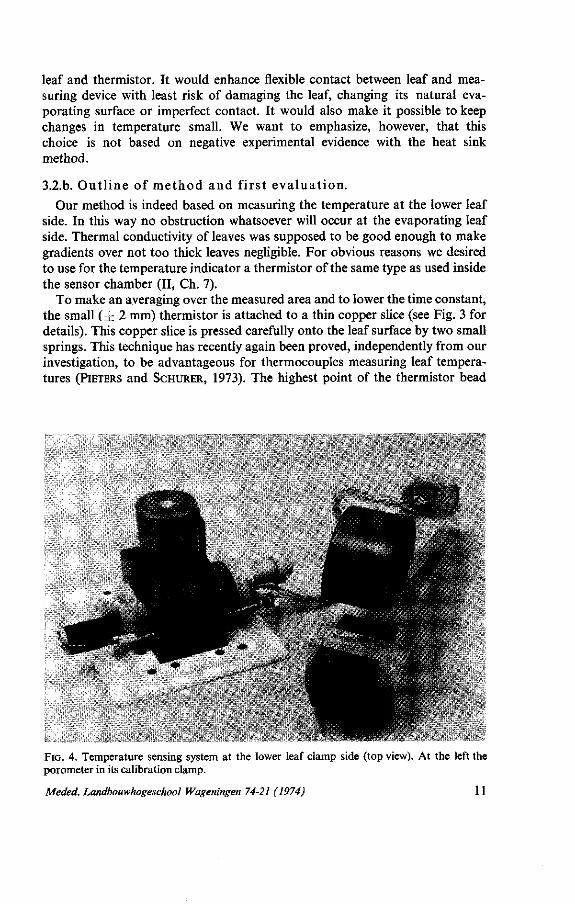
To make an averaging over the measured area and to lower the time constant, the small ( ± 2 mm) thermistor is attached to a thin copper slice (see Fig. 3 for details). This copper slice is pressed carefully onto the leaf surface by two small springs. This technique has recently again been proved, independently from our investigation, to be advantageous for thermocouples measuring leaf temperatures (PIETERS and SCHURER, 1973). The highest point of the thermistor bead

FIG. 4. Temperature sensing system at the lower leaf clamp side (top view). At the left the porometer in its calibration clamp.


surface lays a few tenths of a millimeter above the copper surface, which enhances contact between leaf and thermistor (Fig. 4). During measurements on artificial leaves, bean and corn leaves it was often observed that a minute mark was left at the place (lower side) of the temperature measurement, without any damage of the surface as such. We observed an equilibrium error of 0.3 °C when the wires were not under the copper slice but came straight through the tempex block. We observed also an increased time constant (difference after 15 seconds still 0.5 °C) when the wires were between the copper slice and the lower leaf surface (thus causing poor contact).

The construction as given in Fig. 3 and 4 yielded accurate results. It was firstly tried on artificial leaves made up from a sheet of 0.2 mm polyethylene supporting two wet filter papers between which a rolled thermoelement (STIG-

TER, 1968) was used for temperature indication (Fig. 5). Our choice of polyethylene is based on its relatively high thermal conductivity and heat capacity, compared to other related materials. Thermal conductivity of polyethylene is between 0.35 and 0.5 W/m°C (UNDERWOOD and MC.TAGGART, 1960; KLEIN and KLEIN, 1970) and water at room temperature has a thermal conductivity of 0.6 W/m°C. Heat capacity of polyethylene is ca. 60% of that of water (KOHL-

RAUSCH, 1968; KLEIN and KLEIN, 1970). We therefore believe that the artificial leaf so constructed, with a thickness of 0.5 mm, is a good substitute, for our purpose, for real leaves. This thickness is about 2 to 3 times that of normal non-succulent leaves (e.g. TURRELL, 1965).

From measurements on this artificial leaf we found the time constant of our construction to be about 4 seconds under the conditions described. The thermoelement did even reach the same final value (within 0.2 °C) in less than half the time needed by the thermistor. This latter observation is of importance because it means that eventual changes of the thermistor over the short transient time will be mainly due to adaptation of the thermistor to the already nearly constant leaf temperature (Comp. Ch. 4.2).

We found also that with original temperature differences, measured with the thermoelement and the thermistor, of 3.5 to 4 degrees between the evaporating surface and the air (thermistor) in the room, the leaf part measured changed by 1.2 to 1.5 °C after clamping of the device. So the thermistor bead made two third of the original difference and the leaf part one third.

The original temperature difference between leaf and air may vary between a leaf of 6 degrees cooler to a leaf of even something as between 10 and 20 degrees warmer than the air (e.g. LINACRE, 1964; DRAKE et al., 1970; STOUTJESDIJK,

1970). In view of what has been derived in (I, Ch. 4.3) we can disregard in this connection differences between the two leaf surfaces. Of course the new temperature to which the leaf part to be measured approaches is a result of a complex change in its energy balance. Outdoors a source of radiation energy is withdrawn, the boundary layer and the vapour pressure gradient at the side measured by the porometer are changed. Contact is made with the copper slice and the thermistor, with the clamp and the sealing rubber, preventing evaporation at these very places. At the side measured by the porometer the difference in


FIG. 5. Arrangement for measurements on an artificial leaf.

evaporation conditions depends on two things, apart from the obvious change in the vapour pressure to which it is evaporating. Firstly difference in boundary layer resistance is involved between the situation with the apparatus (1.8 s/cm) and without. The latter depends on wind speed, so outdoors on the height inside the crop, determining the original boundary layer (I, Ch. 4.1). Secondly a new (equilibrium) temperature determines the vapour pressure inside the leaf.

This will all influence the complex time constant of the measured leaf part in our temperature measuring situation. By the way the 'time constant' of the measuring procedure itself may not be constant. We are convinced from our observations that this does not violate our conclusion that time constant effects may be overcome. Although presumably the check we made above is fair under most climatic conditions occurring in the Netherlands, it is difficult to forecast whether the situation measured with the artificial leaf is representative enough for all occurring situations. Therefore we have taken the possibility for measuring a long and a short transient time as a method for checking temperature measurements. This method can also be used in the field. Examples are given in Appendix 4 and Chapter 4. For discussions on the mechanical influences of the temperature measuring device on leaves and further considerations to the effective leaf surface measured by the porometer we refer the reader on Appendix 4.


3.3. INFLUENCES OF THE DEVICE.

Regarding other influences of clamping the device onto the leaf we first repeat what has been derived for this purpose in (I, Ch. 4.4). Because of high internal resistances (vertically and laterally) changes in evaporation conditions of the leaf do normally not influence partitioning of strength of evaporation sources within the leaf in a measurable way. An exception can be expected under stress conditions, as described at the end of (I, Ch. 3.2, see also a remark in MEIDNER

and MANSFIELD, 1968, Appendix A3), but in the case of changing conditions we will in our method again be warned by comparing results of short and long transient times (quotient check, see below, or resitance calculations). This same check can also be used to see whether stomatal opening has changed. If MOR

ROW and SLATYER (1971) are right in stating that stomata are not likely to react 'mechanically' in a very rapid way under most stress conditions, these two causes for a deviation from a constant quotient may be expected to manifest themselves separately (Comp. 3.4).

In general not much detailed information is available on the dynamic behaviour of stomata in plants growing outdoors with their roots in soil (COWAN,

1973). Reasons for stomatal opening to increase or decrease relatively rapidly have normally to be found in changes in light conditions or C02-conditions induced by the device. This is apart from reported effects by responses of stomata to changes in humidity conditions in some species (LANG et al., 1971), which are supposed to be due to peristomatal transpiration. However, these effects have an observed time lag of two minutes before onset. Care must be taken in interpreting observed changes in the quotient, Q, of long and short transient times. The occurrence of natural shadow, from clouds or neighbouring leaves, prior to the measurement on a certain part of the leaf, can also be a cause for a different Q. Especially indoors also the existence or inducement of short period stomatal oscillations (I, p. 10; HOPMANS, 1971) may influence Q. However, in the field such oscillations with periods shorter than two hours have not been reported (HOPMANS, 1971).

As our device darkens the leaf part to be measured, the photosynthesis process will stop. This reaction of the photosynthesis processes is so rapid that eventual reaction of the stomata on a change in the C02-conditions by exhaustion of the porometer C0 2 will not occur (e.g. GAASTRA, 1959). The latter reaction will be developed especially if no light exclusion will take place (perspex sensor chamber) and with a high porometer opening over chamber volume ratio. Drying by internal pellets in stead of sweeping with external dry air may enhance low C02-concentrations under such conditions. Such a lack of C0 2 may produce a wider opening of the stomata (e.g. MEIDNER and MANSFIELD, 1968; contradicting information in HOPMANS, 1971). This will decrease Q relative to its value at constant opening. Bringing the leaf part in darkness may result in closing of the stomata, leading to an increase in Q (Comp. 3.4).

The decisive factor for disturbance of the resistance measurement is the rate of reaction of the stomata on a change in the environmental conditions. A


change in stomatal opening due to a change in C02-conditions, under no stress conditions and without oscillations, seems to take at least several minutes to reach half its new final value (e.g. GAASTRA, 1959; GLINKA and MEIDNER, 1968). Measurements on several different species by MANSFIELD and MEIDNER (1966), MORROW and SLATYER (1971) and WOODS and TURNER (1971) suggest that this is also valid for the response on shading.

On the contrary, this does not apply to well known extremely rapid reactions on sudden changes in water conduction to transpiring leaves (MEIDNER, 1965). This latter effect was hold responsible by SHIMSHI (1967) for immediate changes in leaf permeability observed after clamping of a pressure drop (viscous flow) field porometer on leaves. In this case the external pressure of the gasket rings are curtailing water supply to the enclosed leaf parts. Such reactions have not been observed with our instrument.

Not much is known, regarding C02-effects or effects on changes in illumination, on duration of the lag between stimulus and the first onset of change. Moreover, the reactions on the same stimulus seem to be dependent on external conditions prior to the observation (MEIDNER and MANSFIELD, 1968). Also the endogeneous rhythms may influence susceptibility to stimuli. Oscillations may be quite confusing in the laboratory if one is interested in a momentaneous value. It seems therefore unlikely to be able to exclude or forecast changes of stomatal opening after application of the device. Collection of information regarding the behaviour of stomatal opening during measurements is therefore highly desirable.

3.4. THE QUOTIENT OF LONG AND SHORT TRANSIENT TIMES.

The ratio of long and short transient times, observed over dummy resistances under constant environmental conditions, is theoretically a function of sensor behaviour only. Using (II, eq. 4; see this article eq. 27) it is easily derived that Q may be written as :

(At)i0„g _ „ _ Vf, longjRl, long + Rp) _ , . . .

( L\t)short Kt> short (Jii, short + Rp)

with

l n g| - ep (h)

(-., e l ~ ep (h. long) ,„ U ~lne,-e,(tt)

U)

el - ep (h, short)

For a constant (ratio of) Vt (II, p. 23, 25) for long and short transient times, Q is, for (dummy) resistances with a constant Rt, determined by Q' only (6, 7).


Q' contains the equilibrium water vapour pressures at the evaporating surface and at the fixed electrical resistance points. So at each surface temperature, combined with a fixed sensor temperature, Q' must be a constant.

One may calculate for our sensors that theoretically Q' is hardly temperature dependent. For a sensor at 25 °C and a surface temperature of 25°C the ratio, from (7), is 4.13. Increasing surface temperature to 30 °C, but with a sensor remaining at 25 °C, this becomes 4.09. Both being at 30°C one has to expect a ratio of 4.11.

An example of real experimental values for Q, as measured on dummy resistances, with porometer and heating source at nearly equal temperature, is given in Table 3. Measurements QA1 and QA2 are made on the day after the one on which QB1 and QB2 were taken. Accuracy within each series is between 1 and 2 %. The accuracy of Qmean is better than 1 %. We will deal with deviations from the ideal picture outlined above in Appendix 5. We will show there that the trend of Q with resistance, and a trend we observed in the course of time, might be explained from slight deviations from obeying Fick's law of the porometer itself.

These trends in no way prevent us from using the fixed quotient values for indication of constant stomatal opening in the field. From (6) we see at once that Q is modified as soon as Ri,short and Ri,long are no longer equal. If other sources for a change in Q, such as changing temperatures (influencing Q') or occurring internal resistances under stress conditions, may be disregarded, a quotient value that is not equal to the one forecasted by calibration forms an indication for variations in stomatal opening conditions. Of course from one deviating Q only, we do not know whether this change did occur after the end of the short transient period or already earlier. We will deal with this problem in Chapter 4. Of course the same information as contained in Q is supplied by calculating resistances via calibration V,s and Rps for long and short transient times. Its main advantage, however, is the more direct indication which makes it possible to have immediate information on changing stomatal conditions at hand during measurements.

A check on the forecasting capability of measured Q in calibration series

TABLE 3. Representative measurements for dummy resistances of the quotient Q of long and short transient times for different measuring series at different temperatures. The measurements belong to the series with which the second column of Table 1 was determined.

Approximate Rtm (s/cm) QA1 QA2 QB1 QB2

(21°) (27°) (23.5°) (24°)

2.5 3.0-3.5 3.5-4.0 4.5-5.0 7.0-8.0

12.0

4.13 4.15 4.19 4.18 4.25 4.27

4.00 4.05 4.08 4.16 4.20 4.29

4.05 4.06 4.11 4.15 4.20 4.28

4.00 4.03 4.05 4.12 4.20 4.29

4.05 4.07 4.11 4.15 4.22 4.28


TABLE 4. Check on forecasting capability of the quotient Q of long and short transient times from calibrations before the day of a measurement (Qi and g2) and after that day (ß3 and ß4). The mean of this four calibration series (Qcaiur) is compared with the mean of three measuring series on the "measuring day", Qmeas- The measurements belong to the series with which the values in Table 2 have been determined.

Approximate Rtot (s/cm) Qt Q2 Qi 6* Qcaitbr QmeaS

(21°) (26°) (22°) (25°) (23.5°) (23°)

2.5 3.0-3.5 3.5-4.0 4.5-5.0 7.0-8.0

4.10 4.11 4.19 4.21 4.26

4.02 4.06 4.10 4.17 4.25

4.04 4.08 4.07 4.13 4.18

4.07 4.16 4.16 4.20 4.28

4.06 4.10 4.13 4.18 4.24

4.07 4.10 4.12 4.18 4.25

before and after a measuring day is given in Table 4, using our dummy resistances. The accuracy within the series gi to g 4 is again between 1 and 2 %. The accuracy of the means is better than 1 %.

Finally it must be held in mind, in general, that the fixed starting point chosen (II, Appendix 3), the porometer resistance and the changing properties of a certain sensor in the course of time (II, Appendix 4) do all influence Q and its behaviour. It will be dealt with in Appendix 5 that eventual differences in Rp

obtained from long and short transient time measurements, Vt remaining almost constant, form no problem. We may use separately the respective indications of Vt and Rp as calibration values.

We have added a guide to users of porometers, summarizing the most important points that follow from our investigations, as Appendix 6.


4. F I E L D M E A S U R E M E N T S IN I N D I A N CORN

4.1. GENERAL REMARKS.

The reported field experiments were carried out in the summers of 1972 and 1973, respectively in a 5 ha and a 10 ha field of Indian corn (Zea mays L., variety Caldera 535). The planting pattern was nearly uniform with a row distance of 40 cm and three plants on 1 m within the rows. The experiments formed part of a measuring project set up for experimental checking, by our laboratory, of a climatological submodel within the growth models constructed by the Department of Theoretical Production Ecology, also of Wageningen Agricultural University (I, Ch. 1.3; II, Ch. 1). The results of these checks will be published elsewhere. We will deal here only with the results on exploring crop diffusional resistance.

The experimental fields were situated near Swifterbant in Eastern Flevoland, one of the newly reclaimed polder areas of the former Lake IJselmeer. The corn fields formed part of the 250 ha mixed experimental farm in that area, belonging to the university. A routine meteorological observational station, set up by this laboratory, is situated ca. 1 km from the experimental fields.

4.2. TEMPERATURE MEASUREMENTS.

An important point is the check on the temperature measuring system under the field conditions concerned, as stated earlier. For all our measurements we can describe a general behaviour of the leaf thermistor. Immediately after the moment of clamping the thermistor onto the leaf, temperature decreased, but within 5 seconds or less the trend was reversed, slowing down appreciably after about 10 seconds. This behaviour can be explained from the fact that the original leaf temperature must have been lower than clamp temperature but became influenced by changes in the energy balance that increased leaf temperature.

A quantitative check for correctness of our temperature measurements, under field conditions, could be made by the same method as mentioned in Appendix 4. For a series of field measurements of somewhat more than one hour on corn leaves (Table 5), resistance calculations have been made with short and long transient times respectively. The short transient times were the shortests ever measured in the field, in the order of 5 seconds. This depends on the value of Vt and the opening condition of the stomata. The starting up period, prior to the passage of the first fixed electrical resistance, could under our conditions, as a very good rule of thumb, be taken as slightly longer than the short transient times involved. This means that the second fixed electrical resistance was passed from 10 to 12 seconds after clamping. The first temperature reading made after this passage has to be almost representative for the true leaf temperature


at that moment. Indeed temperatures measured again about 15 seconds later, after passing the third fixed electrical resistance, were as a mean only 0.3 °C higher.

Now we recalculated the resistances with a temperature 0.3 CC higher than the one measured directly after the short transient times. The resistances became on the average only 0.1 s/cm ( < 5 %) lower. These latter values being compared in Table 5 with the calculations over the long transient times, we find a mean difference of only 0.05 s/cm. This is within the existing accuracy limits. Therefore we may conclude, in connection with Appendix 4, that also in the field the leaf must have been earlier at temperature equilibrium than the thermistor. Changes in the readings during and after the short transient times can be mainly attributed to the time lag of the thermistor.

We may now draw the conclusion from the above that under our field conditions the leaf temperature can be measured correctly. For short transient times of about 10 seconds temperature can be determined, within 0.2 °C, directly after passage of the second fixed electrical resistance. For short transient times between 5 and 10 seconds the error made in this way remains small. It may be made even less by comeasuring the long transient time and determining the

TABLE 5. Twenty subsequent measurements on comparable places of corn leaves, used for checking the temperature readings in the field. Leaf resistances calculated from short transient times and long transient times respectively are compared. It is also an example used for showing the forecasting capability of the quotient of long and short transient times under ideal conditions. For elaboration on this see Ch. 4.3. The averages given are arithmetic means.

Short time(s)

5.34 5.64 5.90 5.70 5.61 6.64 6.35 5.08 4.93 7.57 6.22 5.46 5.15 4.80 4.57 4.47 5.20 5.04 4.69 5.10

Averages

Q

3.60 3.57 3.64 3.64 3.61 3.65 3.60 3.59 3.61 3.60 3.60 3.65 3.55 3.59 3.56 3.60 3.62 3.63 3.60 3.64

3.61

Leaf side

U L U L U L U L L U U L U L U L U L U L

Calculated leaf resistances (s/cm)

Short time

2.05 2.20 2.65 2.45 2.20 3.20 2.85 1.95 1.60 3.70 2.80 2.65 2.05 1.85 1.70 1.65 2.30 2.15 1.80 2.15

2.30

Long time

2.00 2.15 2.65 2.45 2.20 3.15 2.75 1.90 1.65 3.50 2.70 2.65 1.95 1.85 1.65 1.65 2.25 2.15 1.70 2.10

2.25


temperature once more thereafter. If still shorter transient times do occur, the long transient times can be used for calculation of the resistances if the same starting up period before the passage of the first fixed electrical resistance has to be maintained.

We used for the measurements of Table 5 measuring places ca. 20 cm from the top of big leaves, near the leaf central vein, in a 1 m high crop. All places were fully sunlit leaf parts. The difference between final leaf temperature and (higher) porometer temperature was as a mean about 2 °C. The variation was mainly due to variation in porometer temperature. The latter hardly changed during a measurement, because of our construction with the anti-convection membrane. It changed, however, somewhat in the waiting periods prior to each measurement. This was due to different environmental influences, although the porometer was protected by a radiation shield from direct solar radiation.

It is interesting to note here in passing that the mean resistance for upper and lower leaf side respectively was 2.3 and 2.2 s/cm (for the twenty measurements quoted). The values in Table 5 therefore give also a first idea of the variability of the diffusion resistance of identical places of different leaves, here under fully constant and most ideal radiation conditions (Comp. 4.4.b).

4.3. CHANGES IN THE OPENING STATUS OF THE STOMATA.

4.3.a. Genera l r emarks .

The forecasting capability of the quotient Q was checked under these constant field conditions by the use of the same measuring results (Table 5). Ratios between long and short transient times were determined from calibrations the day before and the day after the measuring day. They forecasted a ratio of 3.64 ± 0.04. This value is valid for the mean resistance of the subsequent measurements of Table 5, at the mean cup temperature of 27.5 °C. According to Table 5, we measured 3.61 ± 0.04. This means that also for the relatively very low short transient times and low resistances this ratio, which is much lower than the theoretical one (Appendix 5), can be excellently used for checking changes in the opening status of the stomata. The results of Table 5 show that at least within the first half a minute no significant changes were detected.

It must be noted that a quotient Q higher than the one forecasted from calibrations does not necessarily give rise to the conclusion that the short transient time has been measured incorrectly. It may only be concluded that at least after the short transient time something happened to the stomata. We need a large number of measurements to have a more quantitative indication relating device influence on stomatal opening. Only in the cases of naturally changing light conditions one can expect a priori that certain opening or closing trends may be present over the short transient times. As no possibility whatsoever did exist, with other methods in use, to study these points quantitatively, we have paid special attention to them in the following subchapters.

It is useful to notice that in the short calibration method, with one or two


dummy resistances only (II, p. 26), the use of Q as a forecaster remains possible. Its behaviour with changing Rtot must be reconstructed using (6) and by doing one or two measurements over a high dummy resistance for a check on the existing limit.

To collect information on the changing of the opening status of the stomata it is of special interest to measure on days with changing light conditions. It makes measuring however much more difficult since the variability becomes almost unmanagable. This is the more true because of the fact that comeasu-ring of long transient times, under relatively high resistance conditions, does lower the number of measurements which can be made per unit of time with more than a factor two. Suppression of long transient times is permitted with our measuring strategy and in that case measuring time mainly depends on the required waiting periods. The maximum number of about 25 measurements per hour of short times only is decreased to ca. 10 per hour if long transient times are comeasured. The measuring results reported below are therefore in the first instance used for investigation of device influence on stomatal opening. The absolute resistance values have only a very relative meaning as such if not averaged over a large amount of data.

4.3.b. The measu remen t s of 4. VI I I .72 : v a r i ab i l i ty and the r a t i o Q at the t op of the canopy.

A first series of 27 field measurements was done in about two and a half hour in the course of the morning. The light conditions during a few minutes, including the waiting time, prior to each measurement, could visually be divided roughly in three classes. Class 1 with relatively high light, creating clear shadows. An intermediate class 2 'with transparant sunshine' and characterized by the appearance of weak shadows. Class 3 with overcast condition in the sense that no shadows were visible. The measurements were done at a height of between 1.75 m and 2 m on arbitrarily chosen sunlit places (for light class 1 and 2) of large corn leaves in a crop at the end or just over its vegetative period (SHAW and THOM, 1951a) on a moist soil. Measuring places in class 3 were, as far as possible, chosen such that they would have been in full sunshine if the radiation would have been available. The results are shown, again as an example of natural variation, in Table 6. Temperature difference, during the measurements, between measured leaf part and (warmer) porometer was 1.2 °C on the average.

We wanted to use the calibration-g as an indicator for eventual influence of the porometer on stomatal opening. The forecasted Q for this sensor, with a high Vt, was from 4.08 at an Rtot = Rt + Rp of 2.5 s/cm to a maximum of 4.14, at the temperature of 22 °C. This means an expected value at the average resistance observed of 4.12 i t 0.04.

Studying Table 6 we see that Q is much more variable than in the example of Table 5. This is due to the naturally changing light conditions, which bring the stomata in opening or closing trends. If we cancel the extreme Q of the measurements Nr. 9, 20, 21 and 27, the average field-g becomes 4.1 ± 0.2 in accordance with the forecasting. In this mean of course the much shorter ratios


TABLE 6. Subsequent measurements of 4.VIII.72. Average leaf resistance, Ru is 4.8 s/cm (arithmetic mean).

Nr. Meas.

1 2 3 4 5 6 7 8 9

10 11 12 13 14 15 16 17 18 19 20 21 22 23 24 25 26 27

Short Transient Time

16.44 14.34 15.19 20.64 15.46 19.56 13.39 13.31 10.99 18.64 12.70 14.32 18.66 21.83 15.29 15.10 16.01 24.17 23.58 27.06 19.56 15.13 24.49 24.84 26.64 13.09 18.97

Q

3.94 4.22 3.98 4.07 4.17 4.11 4.05 4.15 4.39 3.97 3.99 4.06 3.98 4.06 4.08 4.04 4.16 4.15 4.07 4.96 4.55 4.23 4.07 4.29 4.07 4.17 4.41

Light class

2 1 2 2 3 2 2

3 3 3 3 2 3 3 2 2 2 3

Leaf side

U

u u u u u u u u u u L L L L L L L L L L U U

u u u u

R,

4.8 3.4 3.7 6.0 3.8 5.5 3.1 2.5 2.5 5.5 2.8 3.5 5.2 6.3 3.6 3.6 4.6 7.1 6.8 8.1 5.0 3.4 7.1 7.3 6.1 2.6 5.1

between 3.9 and 4.1 are also involved. They indicate measurements in which a natural opening trend existed, which was not, or at least hardly, disturbed by application of the device.

It is not known whether such opening trends are promoted by the endogenous opening trend in the morning. The opposite effect, an enhancement of the susceptibility for influence by the apparatus on the opening situation, by the endogeneous closing trend in the late afternoon, has been suggested from observations earlier (WALLIHAN, 1964). We have taken it for granted that in the hours of observation, in the late morning from 10 o'clock to 12.30, such an eventual influence of the endogeneous opening would be very small. As we have argued in Ch. 3.3. that our device itself can not provoke an opening trend, we may take now the values of Q schorter than 4.1 as an indication for the influence on Q by the variability of light conditions. As, on the average, periods with increasing and decreasing light will have occurred with the same frequency, the margin for increased Q due to decreased light may be taken as equal to this margin for decreased Q due to increased light.


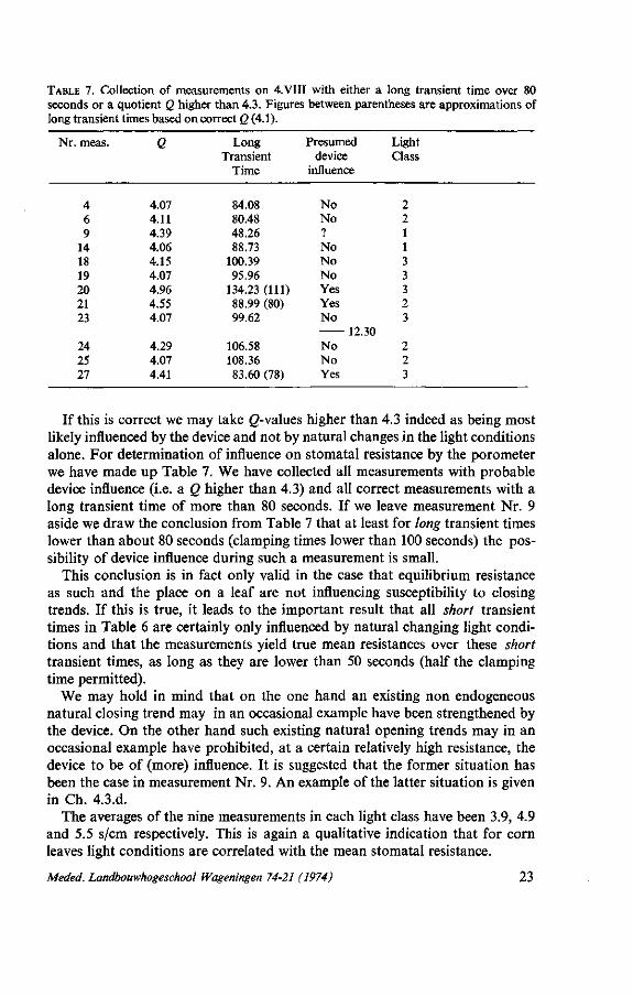
TABLE 7. Collection of measurements on 4.VIII with either a long transient time over 80 seconds or a quotient Q higher than 4.3. Figures between parentheses are approximations of long transient times based on correct Q (4.1).

Nr. meas. Q Long Transient

Time

Presumed device

influence

Light Class

4 6 9

14 18 19 20 21 23

24 25 27

4.07 4.11 4.39 4.06 4.15 4.07 4.96 4.55 4.07

4.29 4.07 4.41

84.08 80.48 48.26 88.73

100.39 95.96

134.23(111) 88.99 (80) 99.62

106.58 108.36 83.60 (78)

No No ?

No No No Yes Yes No

12.30 No No Yes

2 2 1 1 3 3 3 2 3

2 2 3

If this is correct we may take g-values higher than 4.3 indeed as being most likely influenced by the device and not by natural changes in the light conditions alone. For determination of influence on stomatal resistance by the porometer we have made up Table 7. We have collected all measurements with probable device influence (i.e. a Q higher than 4.3) and all correct measurements with a long transient time of more than 80 seconds. If we leave measurement Nr. 9 aside we draw the conclusion from Table 7 that at least for long transient times lower than about 80 seconds (clamping times lower than 100 seconds) the possibility of device influence during such a measurement is small.

This conclusion is in fact only valid in the case that equilibrium resistance as such and the place on a leaf are not influencing susceptibility to closing trends. If this is true, it leads to the important result that all short transient times in Table 6 are certainly only influenced by natural changing light conditions and that the measurements yield true mean resistances over these short transient times, as long as they are lower than 50 seconds (half the clamping time permitted).

We may hold in mind that on the one hand an existing non endogeneous natural closing trend may in an occasional example have been strengthened by the device. On the other hand such existing natural opening trends may in an occasional example have prohibited, at a certain relatively high resistance, the device to be of (more) influence. It is suggested that the former situation has been the case in measurement Nr. 9. An example of the latter situation is given in Ch. 4.3.d.

The averages of the nine measurements in each light class have been 3.9, 4.9 and 5.5 s/cm respectively. This is again a qualitative indication that for corn leaves light conditions are correlated with the mean stomatal resistance.


4.3.C. Measu remen t s of 25. VIII . 72: the r a t i o Q t h r oughou t the c r op . Another 30 field measurements were made mainly in an afternoon, under

comparable conditions as those on 4.VIII, from noon to 12.45 and from 14.00 to 16.30. Results regarding possible device influence are given in Table 8. Again the measurements are on normally sunlit places. Now also height inside the crop, in its reproductive stage (SHAW and THOM, 1951b), was involved.

Forecasted Q was from a mean of 4.19 at 2.5 s/cm to a maximum of 4.23 for the temperature concerned, so with an average of 4.21 ± 0.04. The presumably correct g-measurements taken together yielded, again for the changing natural light conditions, 4.1 ± 0.25. The porometer was on the average 0.9 °C warmer than the measured leaf part, over the short transient time, but for the measurements with a resistance higher than 20 s/cm this was for example only 0.2 °C.

Endogeneous closing trends are again supposed to have small influence. From the results of Table 8 we conclude that with a long time of 90 seconds or lower we can expect to have made correct measurements, which is comparable with the.results on 4.VIII (Table 6 and 7). Only two measurements, with a short transient time higher than 60 seconds (a resistance higher than 20-25 s/cm and a ß > 7), had to be distrusted because of probable device influence on this short transient time. These general statements may be only made, for the time being, if we take it indeed for granted that susceptibility for closing trends induced by the device is again independent of equilibrium resistance and also independent of height in the crop, leaf side and measuring place on the leaf.

The last measurement at the bottom of Table 8 was the first measurement in

TABLE 8. Collection of measurements on 25.VIII with either a long transient time over 80 seconds or a Q higher than 4.35 but lower than 7. Figures between parentheses are approximations of long transient times based on correct Q (4.1). Height classes are: a, from 1.75 m upwards; b, between 1 m and 1.50 m ; c, from 75 cm downwards.

Q

4.17 4.81 4.38 4.24 3.95

4.02 4.62 6.55 6.25 6.13 4.76 4.28 5.12 4.06 3.85

Long Transient

Time

92.90 148.82 (126) 101.27 (95) 126.83 90.92

93.44 128.90(114) 244.57 (153) 261.26 (171) 165.56(111) 108.62 (94) 100.64 187.03 (150) 83.78 83.54

Presumed device

influence

No Yes Hardly No No

12.30 No Yes Yes Yes Yes Yes No Yes No No

Leaf side

L U L U L

U L U L U L U

u u u

Light Class

3 3 3 3 3

2 2 2 2 2 2 2 2 2 1

Height Class

a b b a a

b b c c a b c c a a


a fully sunny period after a long period of light class 2. This immediately shortens markedly the Q concerned, due to an existing natural opening trend. No further comparisons will be made between resistances at several heights and several light classes as the number of measurements in some possible combinations is only 1 or 2. The mean of all measurements (8) in light class 1 was 3.7 s/cm, comparable to the results on 4.VIII. From the measurements on these two days one may conclude that under the conditions concerned influence of the device becomes important only when the device is clipped onto the leaf for more than 1.5 to 2 minutes.

4.3.d. The measurement s of 29 .VI I I , 31 .VIII and l . IX . 72 : again the r a t i o Q.

As remarked earlier, the profile measurements were purposed to serve as part of input, or check of output, of a crop climate simulation model. This model should be tested, in the first stage of the work, under high light conditions. Now 1972 was an awfull summer (BECKER, 1974) with no fully clear sky days. The best days were found in the period from 29.VIII-1.IX. These days were different from the ones reported above and relatively sunny with occasional cloud groups temporarily obscuring the sun fully. The day of the 30th was needed for final preparation of the scanning of micrometeorological data, and 31.VIII and l.IX have been days for the complete measuring program.

We report here again on results regarding the influence of the device on the resistance, now on these relatively sunny days. In the next chapter we return to these measurements, taking them together for a first comparison of resistances throughout the crop.

Table 9 shows, in a special measurement series on 29.VIII, what happens to Q in subsequent measurements on the same leaf in sharply changing light conditions. Forecasted Q for 29.VIII being 4.21 ± 0.04 we found 4.15 ± 0.25 in the field. The sixth measurement in Table 9 is of special interest if compared with

TABLE 9. Comparison of 10 subsequent measurements on the same leaf at the top of the crop under changing light conditions.

Short Transient

Time

16.60 12.90 19.57 13.78 13.32 23.83 45.73 32.34 24.84 18.30

Q

4.24 4.36 4.16 4.18 3.92 5.18 > 7

3.58 4.04 4.64

Leaf side

U L U L U L U L U L

Light class

1 1 1 1 1 3 3 3/1 1 1

Resistances (s/cm)

4.1 2.7 5.2 3.1 3.0 7.1

15.4 9.9 6.9 4.6


TABLE 10. Collection of measurements on 29.VIII with either a long transient time over 60 seconds or with 4.4 < Q < 1. Figures between parentheses are approximations of long transient times based on correct Q (mean value). Light classes are now: 1, sunny place under full sunlight; 3, normally sunny place under clouds; 3(s), naturally shadowed place under full sunlight; 3 + s, naturally shadowed place under clouds, as far as this could be assessed. Measurements after 12.30 are taken as being made in the afternoon. Height class as in Table 8.

Q

4.27 4.06 4.20 5.85 4.34 5.36

4.42 4.51 5.06 6.54 4.63 4.11 4.69 4.21 4.50 4.48 4.36 5.32 4.18 4.16 4.24 5.18 3.58 4.04 4.64

Long Transient

Time

88.41 72.80 75.62

205.10 (145) 75.50

112.52(87)

78.44 (74) 71.86(66)

102.98 (84) 177.08 (112) 103.94 (93) 60.42

119.77 (106) 106.94 61.40 (57) 60.68 (56) 63.65

170.36 (133) 68.88

107.71 70.40

123.44 (99) 115.64 100.40 84.98 (76)

Presumed device

influence

No No No Yes No Yes

1 J

Hardly Hardly Yes Yes Yes No Yes No Hardly Hardly No Yes No No No Yes No No Yes

Leaf side

L L L U U

u Î2.30

L L L U L U L L U L U L U

u u L L U

L

Light Class

1 3(s) 3(s) 1 1 3(s)

3(s) 1 1

3 + s 3+s 3 3 3(s) 1 1 3 3 1 3(s) 1 3 3/1 1 1

Height Class

a b c a a b

c a a b b c c c a a a b c c a a a a a

the ninth. Both yielded the same resistance. In the sixth measurement a closing trend, induced by natural changing light conditions, has presumably been accelerated. This is a situation which was already mentioned as possibly occurring in some cases. In the ninth measurement the presumably almost finished, at least appreciably slowed down, opening trend may have helped the stomata to remain open under the cup. This effect is certainly present in the eighth measurement. Preparing the latter one we observed that less than a minute before clamping of the apparatus on the leaf the full sun did appear after increasing light conditions in the foregoing minutes. The resulting extreme opening trend induced is found back in this lowest ratio Q we ever observed. This is the more striking in view of the high short transient time (i.e. high resistance) involved. It presumably remains true that the resistance measured is a correct indication for the mean resistance which should have existed over the short transient time period without the presence of the device.


In Table 10 we have once more collected long transient times that help us indicating at what time after clamping the apparatus will start to influence the opening status of the stomata. The situation is different from former chapters in the sense that light class 2 (weak shadows) did not exist, but light class 3 could appear in different forms (see heading Table 10). From the measurements concerned we conclude that certainly after long transient times of 50 seconds (about 65 seconds after clamping) or lower, influence is zero. For transient times between 50 and 70 seconds deviations are small.

From these results it followed that only 2 of the 58 measurements on that day could be indicated to yield a too high resistance because of longer short transient times to be attributed to device influence. It schould be noted that long transient times that were going to Q > 7 were not finished. Validity of their

TABLE 11. Collection of measurements on 31.VIII with either a long transient time over 80 seconds or 4.4 < Q < 7. For further information see legend of Table 10.

Q

4.13 4.25 4.49 4.35 4.31 4.23 4.17 4.34 4.71 4.16 4.90 4.21

4.81 4.43 4.69 4.31 4.81 4.22 4.37 3.85 3.96 5.36 4.29 4.20 4.24 5.38 5.91 3.82 4.56 4.01

Long Transient

Time

111.94 88.01

159.68 (148) 117.08 113.73 87.11

100.46 95.18

134.30(118) 101.60 132.38 (112) 122.24

96.14 (83) 97.43

139.99 (124) 101.81 97.51 (84) 89.65 82.07 83.16

101.12 154.22(119) 85.46 88.70 86.18

138.98 (107) 229.40 (161) 112.70 104.23 (95) 85.76

Presumed device

influence

No No Yes No No No No No Yes No Yes No

12.30 Yes Hardly Yes No Yes No No No No Yes No No No Yes Yes No Yes No

Leaf side

U L L L L U U L L U L L

U U L U

u L U L L L L U U L U L U L

Light Class

1 1 3(s) 3(s) 1 1 1 1 1/3 1/3 3 3(s)

1 1 1 3(s) 3(s) 1 1 1 3(s) 1 3(s) 3 3 3 3 1/3 1 1

Height Class

a a b c c c c c b b b c

a a a c a a b b b c c a a b b c c a


TABLE 12. Collection of measurements on l.IX with either a long transient time over 70 seconds or 4.4 < Q < 7. For further information see legend of Table 10.

Q

4.15 4.37 4.34 4.89

4.47 4.24 4.40 4.26 5.57 4.22 4.57 3.61 4.10 4.80 4.75 3.91 5.50 4.81 4.12 4.24 4.16 4.05 4.11 3.82 4.16 4.37

Long Transient

Time

90.58 135.50 100.94 145.04 (123)

89.49 78.65 99.94 76.99

119.80(89) 103.50 79.07 (72) 98.73 73.97

107.12 (93) 151.71 (132) 74.54

141.92 (107) 177.56 (153) 93.49 71.18 71.12 71.84 88.52

103.04 76.64 82.16

Presumed device

influence

No No No Yes

1-) i n I Z . J U

Hardly No No No Yes No Yes No No Yes Yes No Yes Yes No No No No No No No No

Leaf side

L U L L

U L L U L L U L L L L L L U U U L U

u L U L

Light class

3(s) 3(s) 1 3(s)

1 3(s) 1 1/3 3+s 3+s 3 3/1 1 1 3(s) 3(s) 1 3(s) 1 1 1 1 1/3 3/1 1 1

Height class

b c c c

a b a b c c a a a b b b c c a a a b b b a a

short transient times is judged after the results on device influence obtained from other long transient times.

A last question of interest in dealing with Q is whether there is any difference observed between occurring closing trends due to the device for morning and afternoon, as for example suggested by WALLIHAN (1964). One problem regarding this question is that the number of measurements that can be made in the morning of relatively clear days is often reduced by occurrence of dew. Wet leaves make porometer measurements of course meaningless. If we set the end of the morning period at 12.30, the measurements on the relatively cloudy days of 4. VIII and 25. VIII yield no indication of any difference between morning and afternoon. On the relatively sunny days, information on which is collected in Tables 10, 11 and 12, there is indeed a slight indication that closing trends are easier induced in the afternoon than in the morning.

The smallest long transient times in Table 10 are doubtfull regarding proved influence of the device but the largest transient times without device influence are found in Tables 11 and 12 in the morning. For example on 31.VIII (with the


highest number of morning data) the long transient times seem to be correct as far as they are below 100 seconds or even more. This means that clamping times in the order of 2 minutes are permitted under such conditions.

The information contained in Tables 11 and 12 does not add further new conclusions. It confirms what could be derived from Tables 7, 8 and 10 and proves the consistency of our measuring strategy. Transient times between 70 and 80 seconds, for the afternoon, indicating permitted clamping times of about 1.5 minute, are in correspondence with earlier estimates.

Regarding extrapolation of the results obtained above one may think of differences that might rise from inequalities in plant and soil water status. Such differences have presumably not been high in our cases. Quantitative assessment under other conditions is therefore impossible from our measurements. Referring to mechanisms presumably responsible for stomatal reaction (I, Ch. 2) we suggest that such differences may only be striking under really extreme conditions. It is important to note finally that from the data in Tables 7, 8, 10, 11 and 12 indeed no trend whatsoever can be observed in average susceptibility for closing trends, induced by the device, comparing resistances of the same order of magnitude (comparable short transient times) under apparent different light conditions. This statement is applicable to upper and lower sides, to leaves at different heights as well as to places shadowed by higher leaves or clouds.

4.4. RESISTANCE PROFILES WITHIN A CROP STAND.

4.4.a. Genera l r ema rk s .

Two preliminary remarks have already been made regarding the general character of the corn leaf resistances. Firstly we found high variability between our 2 cm2-samples, even under ideal sunny circumstances. Secondly there was clear indication that the leaf resistance was in general strongly correlated with light conditions, in correspondence with existing evidence (TURNER, 1969). In one more example we followed resistance behaviour of the same top of a normally sunlit leaf at a height of 1.75 m, for two periods of one hour, under capriciously changing light conditions over the crop. The crop was at the end of, or just over, the vegetative stage. We found, in the 25 measurements, resistances ranging from 3.6 s/cm to 16.8 s/cm with everything inbetween.

Sampling a dense corn crop as ours, under high light densities, therefore demands a more systematic study of resistances of sunny and shaded parts of the leaves throughout the crop. If it is possible to find more definite relationships of resistance with height, separately for the two categories, knowledge on the partitioning of shaded and sunlit leaf parts, at each height in the stand, would be sufficiënt for drawing accurate resistance profiles. For the crop concerned an unmanagable amount of measuring points can further be avoided in that case. This may for example be important for seasonal all day readings. Our measurements in 1973 were done to collect more knowledge regarding these sample problems.


In first instance we are interested in the variation of actual leaf resistances throughout the crop. The averages made up must give a picture whether or not differences in stomatal geometry and stomatal functioning are on the average depending on side of the leaf, place on the leaf side concerned and height of the leaf within the stand. Our approach has therefore been the following. We have investigated in principle the variability of the resistance on sunlit and shaded places respectively. For this purpose we made up average resistances as the arithmetical mean of measurements, separately for these two classes and for categories within these classes. Variability observed is taken to be brought about by differences in stomatal functioning, because of differences in reaction of the stomatal systems concerned under comparable light conditions, and by differences in these light conditions within the classes. This is apart from obvious but unassessed differences in stomatal and leaf geometry. In this connection one can mention that TURNER (1969) did not measure any correlation between stomatal density and diffusion resistance of corn leaves.

As soon as we want to use the measured resistances for the calculation of resistance profiles, by calculating average diffusion resistance for a certain crop layer (GOUDRIAAN and WAGGONER, 1972), our approach must be different. Now we have to take into consideration that the diffusion from the surfaces takes effectively place as through parallel resistances. To calculate the average flux density we need the average of the reciprocal resistance values. The effective mean resistance is consequently found as the harmonic mean. The harmonic mean is the reciprocal of the arithmetic mean of the reciprocals of the measured resistances. Comparison of the means over a certain period, 'sampling different parts of a leaf, is in first instance only correct if the experimental data are obtained over a period in which no unknown trends of resistance with time do exist.

If trends exist, sampling throughout the crop or crop layer remains valid if for example the means for sun and shade measurements respectively would appear to be not dependent on place on the leaf side concerned, on the leaf side itself and on height of the leaf within the layer concerned. In that case the harmonic mean of a sufficient number of resistance measurements over a certain period of time must in a lot of cases remain, also with existing trends, nearly equal to the arithmetical mean of momentaneous harmonic means existing throughout the period.

In the examples dealt with so far the difference between the arithmetic mean and the harmonic mean is not striking, but of course important for real model calculations. In the example of Table 5 harmonic means become 2.20 and 2.15 respectively. The harmonic mean for resistances such as in Table 6 becomes 4.2 s/cm. We will see at the end of this chapter 4.4 that absolute values of arithmetic means and harmonic means may differ considerably, especially for shaded places throughout the crop, but that the trends in average resistance are not affected at all.

We did not specially investigate during the measurements in 1973 whether the results of the 1972-research (on changes in the opening status due to the device,


as reported above ) were valid for this same crop on the same field under comparable moisture conditions. Because of the very low V, of the sensor we used in the 1973-measurements and the fact that we often measured only short transient times to increase the number of daily measurements, only a few opportunities occurred for checking. These few checks did not indicate any difference with the earlier results.

4.4.b. Again the measu remen t s on 29 .VI I I , 31 .VIII and I . IX.72 : the r es i s tance va lues .

The measurements on 29.VIII, 31.VIII and l.IX in 1972 have been mainly used to check influence of the device on stomatal opening. We reported already that a fair amount of sunny, cloud-shadowed and leaf-shaded places were observed under occasionally drastical changes in light conditions. In our dense crop shadows and sun spots are also moving under wind influence which also enhances variability. Because of these variations, the daily averages of the relatively small amount of measurements in each possible situation will be not completely reliable. To draw some preliminary conclusions we have therefore only collected the arithmetic means for all the measurements on the three days together. Neither the weather situation in general, nor the soil moisture situation, were very different between the days concerned.

In Table 13 we collected information on sunny places. We have to hold in mind that light densities over the crop have been lower and less constant than under fully clear sky condition. The arithmetical means include all measurements with relative much sunshine in the few minutes prior to each measurement.

Apart from the lower side of the lowest leaves, the differences between the means of upper and lower side and over sunny places throughout the crop do not appear to be very high. Only the higher mean resistance of the lowest leaves seems to have some significance.

In Table 14 we collected information on shaded places, without distinguishing whether they were shaded by other leaves or shadowed from clouds. At least for the average of each height class a clear trend to higher resistances

TABLE 13. Averages of resistance measurements on corn leaf parts under high light density on 3 days with occasionally changing light conditions.

Leaf side

U L

U L

U L

Height class

a a

b b

c c

Number of measurements

28 26

14 14

11 12

Mean resistances

3-8l 4.1 4.5)

3 - 1 ) 3 3 3.4)

4-3) 5.7 6.9)


TABLE 14. Averages of resistance measurements on corn leaf parts under low light density on 3 days with occasionally changing light conditions.

Leaf side Height class Number of Mean measurements resistances

u L

U L

U L

a a

b b

c c

6 7

17 16

16 16

6.41 9.01

10.61 9.01

14.91 10.11 12.5

deeper in the canopy does exist. If we distinguish between places where the illumination was less because of clouds and because of leaf shadows under relatively sunny conditions, we find for the top leaves (cloud shadows only) an arithmetical mean of 7.8 s/cm (13 measurements). For the lower layers we find under cloudy conditions 9.7 s/cm (22 measurements) and for shaded conditions 11.9 s/cm (43 measurements).

We may draw the conclusion from these figures that leaf-shaded places have higher resistances than places only obscured by clouds. This may be understood from the somewhat higher mean illumination under the latter conditions. These results suggest that differences with depth between shaded places under high light densities over the crop may be expected to be even higher than those observed in Table 14. Such differences can be understood from changing light conditions with depth as multiple shadowing will occur deeper in the canopy and the overall diffuse light quantity decreases with depth.

The preliminary conclusions formulated above indicate that it is indeed worthwhile to go deeper into the matter of separate sampling of sunlit and shaded leaf parts throughout a crop under high light densities over the stand.

4.4.C. The measu remen t s of 10.VII . 7 3 : sunl i t t op s .

In Table 5 we used twenty subsequent measurements on places 20 cm from the top of big corn leaves, in a 1 m high crop, to demonstrate the usefulness of Q as a forecaster under ideal conditions and the adequacy of the temperature measuring system under the most unfavourable conditions. They were part of a total number of 84 measurements under the same conditions. The arithmetical means of 42 upper side measurements and 42 lower side measurements on the leaf parts mentioned were 2.15 s/cm and 2.30 s/cm respectively.

It is of interest to look at the frequency distribution. We have distributed the readings over 10 resistance classes and the results for upper and lower sides are shown in the histogram of Fig. 6. It shows that even taking samples at the same portions of identical leaves at the top of a crop, appreciable differences do occur in distributions over the two not very different arithmetical averages. This is most striking at the higher resistance part of the distributions


« 15 E c

Î

10

5

°(

-

i .

) f

-—M

.—x-—

I

2

H-... —-X .,

1

3

—ie—«!

—-*—

i H

U

FIG. 6. Histogram of measurements of Rt (s/cm) on 10.VII. Dots indicate numbers of measurements at the upper leaf side. Crosses do so for measurements at the lower leaf side.

concerned. The distributions have equal modes. We feel that from these measurements the conclusion may be drawn that, at least for the tops of the corn leaves in this growth stage, no fundamental difference does exist between upper and lower sides of sunlit leaf parts.

Of course the angle between measured surfaces and the direct solar radiation is a variable included in the measurements. We have nowhere distinguished between leaf parts receiving solar radiation directly or after passage through the leaf.

4.4.d. The measu remen t s of 9 .VII I .73 : sun l i t t ops and base p a r t s .

An additional series of experiments was made as near to the expected dates of the complete measuring program for the simulation model check as was permitted by the weather. A long fair weather spell, lasting several days, at the time the crop had about finished its vegetative period, gave us the opportunity to do this new series of introductory measurements. The first check was made at the beginning of this period, in the afternoon of 9. VIII, investigating existing resistance differences over the leaf. We compared the upper sides of 25 tops and 26 base parts of, at least at these places, sunlit corn leaves at the top of the crop (from 1.75 m upwards). We found as arithmetical means 3.15 s/cm and 3.20 s/cm respectively (Table 15). Taking out the two extremes would make the averages 2.95 and 3.00 s/cm respectively.

A frequency distribution is given in Table 15. Compared with Fig. 6, with only sunlit tops in a low crop, the spread is higher. Therefore frequency distribution tables are preferred to histograms.


TABLE 15. Frequency distributions and arithmetical means for 51 measurements at sunlit tops and sunlit base parts of corn leaves at a height from about 1.75 m upwards.

Resistance class (i?,) Number of measurements

1-2 2-3 3^t 4-5 5-6 >6

Total number

Top

0 16 5 2 1 1

25

Base

4 10 8 1 2 1

26 Average resistance (s/cm) 3.15 3.20

Again we believe that, in spite of differences in the frequency distributions, we may draw the conclusion that no fundamental differences exist on the average between top and base parts of leaves. We suggest that the somewhat more undulated and wrinkled status of the base of the leaves, bringing more variation in light densities and also slight variation in the natural effective evaporative surface and mean vapour path length, is also partly responsible for the differences between the frequency distributions (Comp. Appendix 4).

4.4.e. The measurements of 10.VIII.73: sunlit leaf parts throughout the crop.

To add to the results obtained in the former series we did in one full sunny day 96 measurements throughout the crop on sunlit top, middle and base parts of upper and lower sides of corn leaves. We wanted to compare in this way middle parts of the leaves with top and base parts taken together. We took top and base parts together because we proved their equality at the top of the crop. We hoped to find simultaneously that incorporation of parts of the crop at different height would yield the same kinds of results compared with sampling the top layer only.

We obtained results on 29 places in the layer from 1.75 m upwards, 36 places in the layer between about 1.50 m and 1 m and 31 places from about 75 cm downwards. In Table 16 a frequency distribution is given without taking the distribution over these three layers into consideration.

If we do distinguish between the three layers we find from top to bottom, for all kinds of measurements in each layer taken together, arithmetical means of 2.40 s/cm, again 2.40 s/cm and 2.60 s/cm respectively. This distribution, also divided in upper and lower side observations, is given in Table 17 which may be compared with Table 13.

It is seen from Table 16 that if we take all the measurements on a middle part of a leaf together we find 2.35 s/cm and for top and base parts together we find 2.65 s/cm. The little attention we have to pay to such small differences in these averages is clearly shown by omitting the four extreme values of the 96


TABLE 16. Frequency distributions and arithmetical means (with and without the four extreme values higher than 6 s/cm) for 96 measurements at sunlit places throughout a corn crop.

Resistance class (RJ

0-1 1-2 2-3 3-4 4-5 5-6 >6

Total number Average resistance (s/cm)

Without 4 extremes

Upper

Top + Base

1 10 4 1 2 --

18 2.20 2.20

Number of measurements

• side

Middle

1 17 6 5 1 -1

31 2.35 2.20

Lower side

Top + Base

2 7 1 4 1 -2

17 3.10 2.30

Middle

4 12 8 2 2 1 1

30 2.40 2.05

TABLE 17. Averages (arithmetical means) of the same resistance measurements as grouped together in Table 16, but now distributed over the three crop layers investigated. All measurements are on sunlit places all over the leaves.

Leaf side Height class Number Average Number Average

u L

U L

U L

a a

b b

c c

15 14

19 17

16 15

2.251 2.501

2.001 2.901

2.701 2.501

29

36

31

2.40

2.40

2.60

measurements, as indicated in the last line of Table 16. For the middle parts of the leaves as a whole we find in that case 2.15 s/cm and for top and base parts together 2.25 s/cm.

4.4.f. A balance for the sunlit places. From the measurements reported above one may draw the now more definite

conclusion (Comp. 4.4.b.) that resistance differences of sunlit places all over the leaves and throughout the canopy must on the average be small. The number of measurements to obtain a reliable average is of course determined by the variability as such. This variability is strongly enlarged by the occurrence of a few extreme values, which certainly are no measuring errors but arise presumably from growth deficiencies or other defects in the stomatal system. An additional reason may be that we have accidentally measured places that were intermittently illuminated because of upper leaves moving in the wind. Especially deeper in the canopy this may happen.


If we compare the results of Tables 13 and 17, the difference in leaf resistances all over the stand will for a large part be a matter of better light conditions for the 1973-measurements. It is imaginable that the appreciable differences in the climatic situation under which this same variety was grown, on the same spot under the same fertilizer conditions, did also influence the results in the two years compared (Comp. e.g. SLAVIK, 1973). Neither the soil moisture situation nor the growth stage of the crop have been very different for the measuring days concerned.

The differences between the results on 10.VII and those on 9.VIII and 10.VIII can perhaps partly be explained from possible seasonal trends of increasing resistance, which have recently been reported from a comparable crop as sorghum (SZEICZ et al., 1973). Research on such seasonal trends have not been part of our program. Differences between 9.VIII and 10.VIII are partly due to the differences in observed extremes. They may presumably further be explained from overall differences in light conditions, caused by high clouds on the 9th.

Radiation conditions over the crop were measured by a Kipp solarimeter, automatically integrated by periods of half an hour. It was installed at the Flevoland routine station since the beginning of 1973. Results of mean amount of short wave energy received over the measuring periods on the 1973 measuring days are given in Table 18.

It was not possible to distinguish, for the resistance, between parts of the day. For that purpose the number of measurements involved had to be sensibly larger. We found, however, not the slightest indication that in the measuring time from 9.30 M.E.T. (at the earliest) to 16.30 there was any important trend over the day. Recent reports of diurnal trends on sunlit places (TURNER and BEGG, 1973) were dealing with lower values than at standard noon, but measured at much earlier and much later parts of the day than we did. Indications for slight closing trends have sometimes been received in our shadow measurements in the lowest crop part at the end of the measuring period (after 16.30 until 17.00 at the latest). These trends have been disregarded in search for the daily averages.

TABLE 18. Mean short wave radiation over the crop during the measuring periods for the measuring days in 1973 (global radiation)

Date Short wave radiation over the crop 1973

J/m2s cal/cm2min

10.VII 9.VIII

10.VIII 11. VIII 12. VIII 14.VIII 15.VIII 23. VIII 24.VIII

660 575 625 650 685 675 655 615 425

0.94 0.82 0.89 0.93 0.98 0.96 0.93 0.88 0.61


4.4.g. The measurements on 11 .VIII.73 : shaded leaf parts throughout the crop.

To give proper attention to the shaded leaf parts in our dense crop, we performed on one full sunny day 90 measurements throughout the crop on shaded top, middle and base parts of upper and lower sides of corn leaves. As in the top layer of the crop the number of shaded places is rather small, we compared 18 measurements in that layer with 40 measurements in the middle layer of the crop and 32 measurements in the lowest stand layer. Results are given in the first columns of Tables 19 (arithmetical means) and 24 (harmonic means). It is clear that the variability is again high. No significance can be attached to averages of a few measurements only. To obtain a somewhat reliable average we can only take together all measurements for this day in a certain crop layer. This yields for the arithmetical means: 8.10 s/cm (6.60 upper sides, 9.65 lower sides of the leaves) for the top layer; 14.45 s/cm (13.75 upper sides, 15.15 lower sides) for the middle layer; 31 s/cm (27 upper sides, 35 lower sides) for the lowest crop layer.

It is clear that we have shown now more definitely than was possible from the 1972 results that the resistance of shaded places is becoming higher, on the average, deeper in the canopy. Whether upper and lower side results may give rise to the conclusion that lower sides of shaded leaf parts have a higher resistance, is at least doubtfull. The number of measurements involved is small. We will see trends changing if we are reporting on averages of more measurements. Differences over one side of a leaf could certainly not be assessed reliably by these measurements.

4.4.h. The measurements of 12.VIII, 14.VIII, 15.VIII, 23.VIII and 24. VIII .73: shaded leaf parts throughout the crop.

We have used all other suitable measurements of 1973 to find out, just as for sunlit leaf parts, whether systematical differences over a leaf do occur and to have an idea of the reliability of the averages on 11 .VIII for the different crop layers. We tried out a special sample scheme on 12.VIII, based on our experiences so far. This scheme we used also in the 4 overall (simulation model check) measuring days that followed (14.VIII, 15.VIII, 23.VIII and 24.VIII).

The scheme is outlined in Table 20. It was based on the facts that we had already a lot of information on sunny places and that in the upper layer sunny places are dominant. As in this layer shaded parts are essentially occurring at base parts of the leaf, we have after 11 .VIII no longer distinguished between different leaf parts in this upper layer but sampled at random. In the middle layer we have made about three times as much shadow measurements as readings on sunny leaf parts (Comp. Tables 19 and 22). On the upper leaf sides in this layer we wanted, after 11.VIII, to find the influence on variability of a double amount (compared with lower sides) of measurements on the same kind of shaded leaf parts (middle parts). On the lower leaf sides we wanted to compare two different places on a leaf. We have chosen the middle parts, heavily measured at the upper sides, and the top parts. The 6 base part measurements


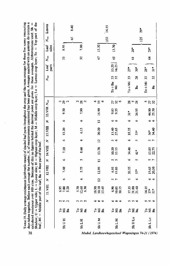
3 tö s ' 3 43 s ? 8 -*•§

«

c/i ç

'S .9 to .2 CS >

S 2 •2£

u ^ bo es

C3

a a o H

a o

ta ta u u g

où en

1 i l S ! > ~

T3

ta M . 2 a a M

S 8 2 O ,£> t a

J3 ta a " 43 'S

O

3 T3 o 2

1 » É a a 8^

2 2 3 S

rs 13 fc!

ta

I s a «S;!-« o < O

§ "e 'S

.a a *° I ü 8

• - . M u 3 gm

JS hH

"S 2 » ta

a <u S3 a

i-J ta

->£ c 5 ta ffl

c s (1> w > <D ta j 3

0 a w

à » S _< en "3

o

tu a a u a>s3

H T3

IS ta <s

co .S

38

> ta

-J 3

•sa s

o

£ t 4 - <2 t a u » 3 »J a

o

> e n CS

^

h-1 > »ri

^ l-H h-(

>

^

> es —H

^

>

^

o 0 0

i n VO

i n

°! 0 0

en

M o \ r ) es

O •n o\

vo

o es i n

VO

o

t~

vo

o r-°

VO

m O O

vo' r»' »n

es v-> es

£ § *

t o

o 0 0

(S

N w N es

O <3\

t ~

vo

i n

VO

VO

s od

V~)

»n

^O

o o o t ^ ^D m >o r j \D

M " O M

E2S ^

te

CO

i n i n

es en

O en i n —H

r-VO

i n

o

y j

f S

o es Ö

rs

O t-; f n

5

oi

rs

O O m 0 \ « * oo' Ö e'i

\ 0 oo \ D

o * M ta

CO

o rn

O i o r s r s

r i r s c r i m

ta

H

<~ r s *o r s rn

>n v-i oo rn «K CT\

vo ^o

O >^l

en r- « rs

VI v o

O " ^

Ó «n

v - i V - l

os o vo «

un r^

O v n v i Ov O » H

vo ö d

vo 00 vo

F2§â

2 -J J3 CO

* rs

r s

# 0 0 rs

vo

* # r- o rs m

(^1 0 0 m r s

ï -

oo t n oo rs rs

in

—i vo m r s

vo vo

m. * oo m - * en

vo m

o • * *

e n T } -

VO v - i

>n

^ * o r~ es en

>n vo

>n o O en oo Tf

m es es

W V I v o

H S pq

o

co

# ON es

vo

* * 0 0 - H rs en

es es en en

! -+ PP o H v i r^ r s

r s en

O O 00 v~± rf in • * es

VO VO

O * • *

vo - * en en

vn r^

i n W1 0 0 I - ;

en rs' - H es

i n t ^

in o VO » H OV Ó - H es

vo vo

i n " î * * T t t - - H ^H m iri

vt »n vo

o M ta

H 2 B

o • J

J3 co

2 H


TABLE 20. Detailed sampling scheme used on measuring days from 12.VIII onwards. Meanings of abbreviations are given in the legends of Tables 19 and 22.

Light Leaf side Crop layer Leaf part

1 2 3 4 5 6 7 8 9

10 11 12 13 14 15 16 17 18 19 20 21 22 23 24 25 26 27 28 29 30 31 32

Sh Sh Sh Sh Sh Su Su Su Su Su Su Sh Sh Sh Sh Sh Sh Sh Sh Sh Sh Su Su Su Su Su Su Sh Sh Sh Sh Sh

U U L U L U U L L U L L U L U L L U L U L L U L U U L U U L U L

H M M Lo Lo Lo M M H H H H M M Lo Lo H M M Lo Lo Lo M M H H H H M M Lo Lo

-Mi Mi To Ba Mi To Ba To Mi Ba -Mi To Ba Mi -Mi Mi To Ba Mi To Ba To Mi Ba -Mi To Ba Mi

of 11 .VIII have been added to the latter. Regarding the lowest layer the amount of sunny places is smallest, which may reduce the number of data to be collected. We have measured between five and six times as much shaded places in this layer. Here we compared top and base parts on the shaded upper sides and middle and base parts on the shaded lower leaf sides.

The scheme of Table 20 gives the detailed sequence. We tried to go three times through the scheme on a measuring day. Only on 14.VIII we missed the last five measurements. The measuring day 24.VIII was not representative enough to use its values, because of frequently occurring clouds (Comp. Table 18). Our experience reported in 4.4.b. regarding leaves shaded by clouds or by other leaves under sunny conditions had made us cautious to include these results.


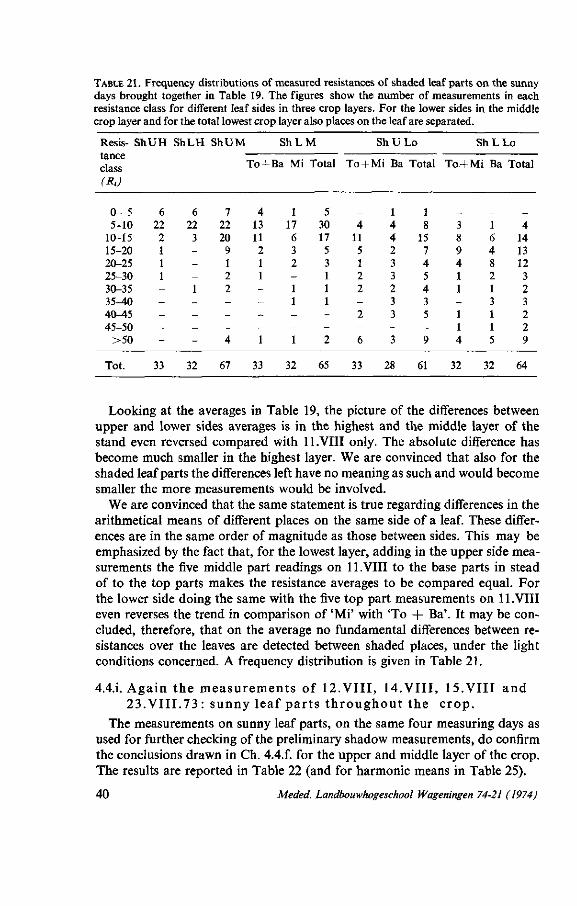
TABLE 21. Frequency distributions of measured resistances of shaded leaf parts on the sunny days brought together in Table 19. The figures show the number of measurements in each resistance class for different leaf sides in three crop layers. For the lower sides in the middle crop layer and for the total lowest crop layer also places on the leaf are separated.

Resis- S

tance class (Ri)

0- 5 5-10

10-15 15-20 20-25 25-30 30-35 35-40 40-45 45-50

>50

Tot.

h U H

6 22 2 1 1 1 -----

33

ShLH

6 22

3

---1 ----

32

ShUM

7 22 20

9 1 2 2

---4

67

S h L M

To + Ba Mi

4 13 11 2 1 1

----1

33

1 17 6 3 2

-1 1

--1

32

Total

5 30 17 5 3 1 1 1

--2

65

S h U L o

To + Mi Ba Total

4 11 5 1 2 2

-2

-6

33

1 4 4 2 3 3 2 3 3

-3

28

1 8

15 7 4 5 4 3 5 -9

61

S h L L o

T o + M i Ba Total

3 8 9 4 1 1 -1 1 4

32

1 6 4 8 2 1 3 1 1 5

32

4 14 13 12 3 2 3 2 2 9

64

Looking at the averages in Table 19, the picture of the differences between upper and lower sides averages is in the highest and the middle layer of the stand even reversed compared with 11.VIII only. The absolute difference has become much smaller in the highest layer. We are convinced that also for the shaded leaf parts the differences left have no meaning as such and would become smaller the more measurements would be involved.

We are convinced that the same statement is true regarding differences in the arithmetical means of different places on the same side of a leaf. These differences are in the same order of magnitude as those between sides. This may be emphasized by the fact that, for the lowest layer, adding in the upper side measurements the five middle part readings on 11 .VIII to the base parts in stead of to the top parts makes the resistance averages to be compared equal. For the lower side doing the same with the five top part measurements on 11.VIII even reverses the trend in comparison of 'Mi' with 'To + Ba'. It may be concluded, therefore, that on the average no fundamental differences between resistances over the leaves are detected between shaded places, under the light conditions concerned. A frequency distribution is given in Table 21.

4.4.i. Again the measurements of 12.VIII, 14.VIII, 15.VIII and 23.VIII.73 : sunny leaf parts throughout the crop.

The measurements on sunny leaf parts, on the same four measuring days as used for further checking of the preliminary shadow measurements, do confirm the conclusions drawn in Ch. 4.4.f. for the upper and middle layer of the crop. The results are reported in Table 22 (and for harmonic means in Table 25).


Ci * '

o o\ V " "

2 Ji X •£> >. «s es H

o L. 3 " O

£ C 3 CD

g J? S <U fa JB >1 w

0 F § 1 t-i +-» 3 Ö

o o ois 4 ^ T 3

50 O

S3 S > >

s -° cd cd

D . T 3 O o

S c *"* cü

3 • £ o M

a c bj} cu 3 (L) o •£> S c«

1 " 03 CL u < - Ü 4 - (U 03 CÎ

Si *-

5 s e o 3 O w « o s

03 s -<U 3 C wi

E o Ä w. " ä <D

se a> C

S 'S

d» cd t - t -

cd * h J S u o > cd t e u

l<2 u ^ " m g

« 1 , " ^ O 3

E/3 0)

cd CL»

- J

fc. £

CS o U T 3

- ) 'S

_ O

ï*

cd t î

" J ft

S

£

_ O

£ ^ HH

> m <N

^

K > vï

%

H > • *

fe;

HH

> t N

%

i n

r-t N

m t ~

. O * o

< s

o m

i n O VO v o

t N t N

T j - t N — i t N

ca PO

t 's o t -

t N t N t N i - i t N

i n O m 0 0

"•cf m '

t N VO

O O i n t N 0 0 Ô

t N - i t N

M >C H

i n i n © i n t N o o

t N t N i -<

V-> T j - - H

O i n t N m

t N t N

e i v o

f - Z c q

a 3 3

t / l

« n CJ\

t N

t -m

O v~i O o o

r ó t N

Tf- f - i — i t N

S 4 - cd

o H

t N t N m « t N

O i n t N o o

• * t N

T t »O

O > n o r ^ t N > o

t N t N t N

m ^ H i r i

O O O n m ^

r n t N en '

t N i - i * C

O O r^ l ^ O

t N t N

r * l ^ o

O M c j

h S f f l

X J 3

t Z l

O t ~

t N

0 0 • *

„

v~,

o t N

> t N

i - i t N - i t N

i n O VO VO

t N • *

•>t t N

e n r n

rn

^D

O o

t N

Ô

i n i n t N • *

t N t N

» n T H

O M cd

H 2 PP

S 3 3

1/3

O • n

t N

• * t N

m ^ H t N

O OV

~H

VD

O M -

t N

Ô

O o I - • *

i - i • *

i - i i n

O v - j l ^ c »

-• "

t N • *

i2s«g

s j

3 VI

i n » n

e n

tn t N

. « n > n

e n

m

^

t N i - i i—l

i n m

t '

m

i n t N

i n '

m

vt o m m

t N t N

t N — i

x n Ô

t N

•tf

O M cd F- 2 PP

o -J 3 3

1/5

O v o

t n

o *

o ^

• n 0 0

t N

t N

i n r~

t N

m

• n

•* • n '

m

i n O N

t N

t N

O M cd

H 2 eq

o

J 3

C/3


TABLE 23. Frequency distributions of measured resistances of sunlit leaf parts on the sunny days taken together in Table 22. The figures show the number of measurements in each resistance class for different leaf sides in three crop layers. For the highest crop layer also different leaf parts are distinguished.

Resistance

class (Ri)

0-1 1-2 2-3 3 ^ 4-5 5-6 > 6

Total number

S u U H

To+Ba

5 6

-3

--

14

Mi

10 5 3 3 1 -

22

1

Total To + M

15 11 3 6 1

-

36

3 7 1 1 2

-

14

Su L H

i Ba

7 6 6 3

-1

23

Total

10 13 7 4 2 1

37

S u U M S u L M S u U L o S u L L o

8 8 2 4 1 1

24

1 11 9 2

--1

24

4 1 5 4 1 2 1 1 1 1 1 1

13 10

Regarding the arithmetical means, the somewhat higher mean value for these days compared with 10.VIII can not be explained from differences in overall light conditions (Comp. Table 18). A trend over the ripening period can hardly be a cause. Comparing, however, the values for upper and lower sides, differences in frequency distributions (Comp. Table 16 and 23), also because of the lower amount of data on 10.VIII, are most likely to be again the most important reason.

A trend for higher resistances in the lowest crop layer, for which there was already an indication in the 1972-measurements but a too slight indication on 10.VIII, is stronger in this case. The most obvious reason is that sunny places lower in the canopy are hardly constant sunny places, due to wind induced movements of many shadowing leaves. This effect indeed becomes much more important deeper in the canopy (Comp. DESJARDIN et al., 1973). Light intensity differences because of the penumbra effect may enhance the effect mentioned (MILLER and NORMAN 1971). Differences in wind effects or occasional measurements in more open spots here and there occurring in the crop may explain differences in influence of the mentioned effects between measuring days. We have not studied more closely leaf parts in higher layers that were submitted to intermittent light because of plant movements in the wind. In these layers intermittently illuminated leaf surface occurs much less frequently.

4.4.j. Some conc lus ions and the way of use of the r esu l t s ob ta ined in the c rop c l imate s imula t ion mode l .

Our final conclusions can be formulated shortly. It is clear from the results of arithmetical means reported above that for the corn crop under research a separation of sunny and shaded leaf parts in the determination of resistance profiles is useful. Sampling them separately and taking into account, with the choice of the number of measurements of each kind, that the resistance of shaded


places changes appreciably more with depth than the resistance of sunny places, seems to be the best approach. It is extremely important that in this way on the average no indications were detected for fundamental differences between different measuring places over the leaves.

Using the values in a crop climate simulation model, it is of interest to compare the absence of principal trends over parts of the leaves as observed in arithmetical means with the outcome of harmonic means (Tables 19 with 24 and 22 with 25). A good measure for comparison is formed by the differences for upper and lower side averages with the total averages for the layer concerned. Regarding shaded places for the highest crop layer and the middle crop layer harmonic means lay closer to each other than arithmetic means. For the lowest layer the reverse is true. Looking at different places over the leaf the arithmetic means are closer to each other.

The restricted value of these differences becomes clear if we look at the base parts measured on 12.VIII (Table 24). In the harmonic mean 6.30 s/cm there is one measurement of 1.25 s/cm, presumably a place which had been accidentally in sunlight before measurement. Cancelling this measurement we bring the harmonic mean on this day to 33.60 s/cm (!). For the now 27 base parts we find a harmonic average of 19.85 in stead of 13.00 s/cm and for the now 60 upper side measurements we get 17.30 s/cm in stead of 14.30. The overall harmonic mean for the layer becomes 18.10 s/cm. Again we have been troubled by an extreme value within the frequency distribution concerned.

Regarding sunlit places (Tables 22 and 25) only differences in the absolute values are worth mentioning. Trends appear to be of the same order of magnitude for arithmetic and harmonic means.

We therefore want to draw the conclusion that sampling methods do not need to be different in obtaining reliable harmonic means. One is inclined to conclude from all the tables with our measuring results that the absolute minimum amount of measurements, under our conditions, is somewhere between 25 and 75. In this way a reliable average, within about 10% of the true mean, can be expected. For sunlit places only the lowest layer possibly needs separate sampling. Within these rough boundaries the number of measurements depends of course on frequency distributions and occurring extremes within the distributions. The final number of measurements, to be chosen in each class of measurements needed, ultimately depends on the expected relative importance in the harmonic mean resistance of the layer concerned and on the accuracy wanted.

It is somewhat surprising that measurements on 50-150 cm2 (porometer opening is 2 cm2) leaf surface could be representative. However, this does not mean that a leaf surface of between 50 and 150 cm2 of one leaf would be representative for the crop as a whole. A random sampling procedure at different leaves and different places on a leaf remains necessary. One has to be aware, for instance, on differences in illumination or stomatal geometry averaged out by our sampling technique to see the truth of this statement.

Having estimated the needed number of random measurements, necessary for


co "

ï o i N

60 ÜJ U S » 1 •* H .S .S <*- _ ~ O SS £ <* " & T 3 • -JS g M

T3 « u . 60 i ->J U « G ~~ -»-C <U cd 3 J3 J= tfl * J *•*

».SS

•- § 2

T3 S «5

ft O

U .a o

3 „ O S

ja A M JO 3 cd O

cd

"g 3

u 1 -o O ja * S

s ^ sS g. ü?53

cd M O Ja a * •a g -o •o o « » ä *-< ca vi •S J5 g is i~r "o «2^ § 'S1'S » ^

e

H S M

0\ ,_,

e s H -

S E S

u 5 S?J5

S

S e 1 3

* u « i j J3 6 ' 3 " J3 D D !3

. cd J

ï S « U > -a cd a

H g.S

44

Vi

cd

2

* 4 - SO

H4 '35

o

£

•J ft

£

> rr,

^

> i n

^

>

fe;

>

^

>

fe:

o VO

vo

i n OV

vd

m m

>n 0 0 0 0

vo

o

av

VO

O

vd

vo

o I N p ^

vo

m

i n

ov

O M cd H 2 m

X O J3

m

vo'

m

•* l ~

VO

S VC

VO

i n

0 0

m

•n

i n

VC

o

vö

OV

O ~ cd

H S PQ

ac - i J 3 CO

O

OV

vo

O

OV

CN

m

" ( S

o OV

S

m

Ö

? t ~

S

S U S

s D J = c«

i n

00*

e n

oô

VO

' •

O VT) 0 0 CN

r~ ov

m CM m m cd

03

+ 's O

f -

m en

oô p

VO VO

»ri S r i ri-'

m VO

O O e n m

i o Ö

• o > o

m est

vo ' OV

v o r ^

o o

oô K

<N oo

H PQ S

S -J J 3 CO

O

•*

VO

.—-—. vo p «ri m'

m oo

o w

f n o o

^O v o

OO ^ H

» ' r

o «n

O O r<1 f N

^O m

«o o

Ó ^6

V I v o

S 8 vd vo

O vo

O M cd

o - J

D JS CO

i n <N

vd

«n es

O

«n vo oô

VO

.—-—. i n ' n i n m vd «

rs CM

_ i _ ed ^ CQ O ^

H

V I o 0\ 0\

tri Ö

\Q \o

v~i » r i * 0 r ^

*n t~-

yr> o

^H v~i

» n ( ^

T t 00*

VO v o

i n o

^6 CÂ

O vo

Sa o

hJ hJ JS CO


Zei o <N T3

Ä

c«

8 • " 23 M ° S <» T3 'S ?? « 9

ca S -o

1 1 II? tri cd d g.H

s 3 a* u

>> cd •

S e s o 2 '•S . « ca ta

1 O > T3

O fc- j -

*j ca <a 9 T 3 T 3 2 8 o •â!=> 2 s . 2 o e u 'S > a w M 3 ï r. «

's-0 § t) « a

•2 g H

d Ö o cl - R § .a ë

1 Ë s rf O G ,^' S -5 v) Ç2 .tS 8 cä LH

ä * i Ë ^ U -O %

2 I-s O d d

«ï

> •

C3 U

i-l

ï*

ca l-l

£

(/) 0)

T ï tyj

N ca

tN

S s *a .22

o

'<

r4

• *

C3 pq

+ 0 H

>/-i

CN

CN CN

S

V }

CN

•*

S + O H

o

m

ca

o »n rn I-H

• *

IT) 5 CN'

o

E-H

;> ' t

o o CN

0\

«

i n • *

Ol

o r~ tN CN

O cd ' « PO 2

O H Sffl

3 od

ä-s«s H so Meded. Landbouwhogeschool Wageningen 74-21 (1974)

X • J

3 &0

S i s *

p 3

05

CN

o M ca H S PQ

o

3 CO

o

CN

o M ca H S PQ

o

45

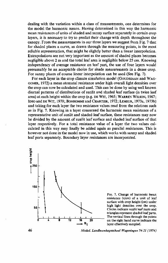
dealing with the variation within a class of measurements, one determines for the model the harmonic means. Having determined in this way the harmonic mean resistances of units of shaded and sunny surface separately in certain crop layers, it is necessary to try to predict their change with depth throughout the canopy. From the measurements in our three layers we suggest from Fig. 7 that for shaded places a curve, as drawn through the measuring points, is the most reliable representation, that might be slightly better than a linear interpolation. Extrapolations are not very important as the amount of shaded places becomes negligible above 2 m and the total leaf area is negligible below 25 cm. Knowing independency of average resistance on leaf part, the use of four layers would presumably be an acceptable choice for shade measurements in a dense crop. For sunny places of course linear interpolation can be used (See Fig. 7).

For each layer in the crop climate simulation model (GOUDRIAAN and WAG

GONER, 1972) a mean stomatal resistance under high overall light densities over the crop can now be calculated and used. This can be done by using well known diurnal patterns of distributions of sunlit and shaded leaf surface (is twice leaf area) at each height within the crop (e.g. DE WIT, 1965; WARREN WILSON, 1967; IDSO and DE WIT, 1970; BONHOMME and CHARTIER, 1972; LEMEUR, 1973a, 1973b) and taking for each layer the two resistance values read from the relations such as in Fig. 7. Knowing in a layer concerned the harmonic mean resistance of a representative unit of sunlit and shaded leaf surface, these resistances may now be divided by the amount of sunlit leaf surface and shaded leaf surface of that layer respectively. For a total resistance value of a layer the two values calculated in this way may finally be added again as parallel resistances. This is however not done in the model now in use, which works with sunny and shaded leaf parts separately. Boundary layer resistances are incorporated.

,250

150

50

J I I L 12 16

J l_ 20

«I

FIG. 7. Change of harmonic mean resistance (s/cm) of a unit of leaf surface with crop height (cm) under high light densities over the crop. Circles indicate sunlit leaf parts and triangles represent shaded leaf parts. The vertical lines through the points on the right hand curve indicate the layer effectively sampled.


Our results obtained with this method will be published elsewhere in cooperation with the Department of Theoretical Production Ecology of this University.

We feel to have improved considerably with our sampling method the former method of introduction of stomatal resistance change with depth in the canopy (GOUDRIAAN and WAGGONER, 1972). Firstly the latter method was based on extinction curves of mean observed visible radiation within a corn crop. This averages out incorrectly the differences between shaded and sunlit places. Further three points were used of a questionable curve, relating stomatal resistance change to illumination measured by a silicon cell. Between these points linear extrapolation was practiced. The curve was taken from literature on an other corn crop.

Because linear relations of stomatal resistance with absorbed light are unlikely to exist, this procedure may give rise to appreciable errors, even apart from the problems of spectral quality of the light concerned. Trying to average out for a certain crop layer the influence of differences in illumination within the classes of sunlit and shaded leaf parts, by sampling, must necessarily be a more promising approach. Other factors are now also included.

Using one curve as in Fig. 7 for the change of resistance with depth in the canopy is implicitly based on an assumed equality of the extinction of diffuse light over the day. Regarding diffuse sky radiation this seems to be valid. A proof that the assumption is also valid for radiation diffusely scattered by the leaves comes, for a corn crop, from the almost constant albedo over most of the day (IDSO and DE WIT, 1970).


5. S U M M A R Y

We report in this closing publication, in the series on leaf diffusion resistance to water vapour, on experiences regarding the use of the improved diffusion porometer. Its detailed description was given in the foregoing article.

We firstly deal with an improved evaporation measuring method to determine independently the diffusion resistance of the nickel perforated membranes used as calibration resistances. The results of these measurements are compared with values from a calculation method, estimating resistances of membranes with funnel shaped holes, as given by PENMAN and SCHOFIELD. Their approximation for the pure pore resistance, without the end effects, is excellently confirmed by a new mathematical approach adapted to the shape of our holes. The nickel dummy resistances are finally used for checking the validity of our porometer measuring strategy.

Further we deal with problems encountered in measuring leaf epidermal resistance with our porometer. We report firstly on growth chamber and preliminary field checks of the leaf temperature measuring system on artificial and real leaves. Secondly we demonstrate in an introductory field check, in Indian corn under ideal climatological conditions, the use of the ratio of long and short transient times, measured by the porometer. This ratio indicates the absence or occurrence of device influence on the state of opening of the stomata.

No possibilities have been reported so far for this latter investigation on a routine basis. Therefore we report here on research regarding influence of the porometer on the opening state of the stomata. For this purpose we performed a number of field experiments in Indian corn under relatively constant and under changing natural light conditions. Results for the corn under study indicate that during the morning clamping times from about 2 minutes are permitted without influencing stomatal opening. In the results for the afternoons indications are found that these values are lowered somewhat to about 1.5 minute. No influence could be detected of the actual measuring place in the crop or of the given steady light condition prior to the measurement.

From the same series of measurements preliminary conclusions were drawn regarding the leaf resistance of sunlit leaf parts and shaded leaf parts throughout the corn crop. From the results obtained it appeared worthwhile to go deeper into the problem of determining stand resistance profiles by crop sampling systems for sunlit and shaded leaf parts separately.

The results obtained by several sampling systems indicate that in the crop as a whole no fundamental differences do exist in arithmetic and harmonic mean resistances for sunlit leaf parts. For the times of the day involved in our measuring sequences this appears to be true for different leaf sides and for different places on one leaf side at the same height in the crop. Regarding the relationship with height only in the lowest crop layer investigated, below 75 cm, there was an indication for somewhat higher mean resistances of sunlit leaf parts than


in the rest of the crop. This is presumably due to the higter contribution of intermittently illuminated leaf parts and occuring intensity gradients due to pe-numbral effects.

Regarding shaded leaf parts, again we found that no fundamental differences appeared to exist in arithmetic and harmonic means at any height of whatever places on a leaf chosen. By taking enough samples on the same kind of leaf part in a certain crop layer the influence on leaf resistance of different illumination, and of differences in stomatal functioning and geometry, seem to be averaged out. The change of the arithmetic as well as the harmonic mean with depth is shown to be appreciable for shaded leaf parts, due to changes in mean diffuse illumination with depth.

The harmonic means for sunlit and shaded units of leaf surface respectively, determined by a correct sampling system in each layer, and the determined relationships with depth in the canopy, can now be used in combination with known distributions of sunlit and shaded leaf parts. This is an appreciable improvement for the determination of crop resistance profiles to be used in crop climate simulation models.

It may finally be emphasized that the reliability of the improved porometer used has been felt to contribute appreciably to the validity of the conclusions drawn from our leaf diffusion resistance measurements throughout the crop concerned.


6. ACKNOWLEDGEMENTS

The authors are again highly indebted to Prof. Dr. Ir. J. Schenk and Prof. Dr. Ir. C. T. de Wit, heads of Wageningen University departments of physics and meteorology and of theoretical production ecology respectively. During preparation of the publication of our results they have commented and highly improved our presentation.

Again much valuable help was given at many occasions by Mr. A. E. Jansen and his cooperators Mr. W. C. A. M. Hillen and Mr. T. Jansen of our mechanical workshop. During preparation, carrying out and working out of field measurements with the porometer, enthousiastic cooperation of staff members of our laboratory was never called upon in vain. This applies especially to Messrs. P. Jansen, A. Verhaaf and A. D. Welgraven and equally to the undergraduate students H. B. M. v. d. Ham, L. v. d. Neut and D. Verwaart.

We are grateful to the staff of the Agricultural University Experiment Station at Swifterbant (Flevoland), headed by Dr. Ir. E. G. Kloosterman, for giving us the possibility to carry out the work reported in specially prepared corn fields. For doing preliminary instrument checks we were able to make use of corn fields at the experimental farm Sinderhoeve (Renkum) and at the experimental terrains near the department of horticulture of this University. We are most thankful for these possibilities and for the cooperation in this respect of the Institute for Land and Water Management (I.C.W.), notably to ing. C. Ploegman, and to Dr. Ir. P. A. M. Hopmans of the horticultural department, respectively. It was a pleasure to cooperate with Drs. H. Lof of the theoretical production ecology department in the reported experiments in the I.B.S. growth rooms.VECO-Zeefplatenfabriek N.V. (Eerbeek) advised us skillfully regarding the nickel membranes.

The manuscript was again made ready for printing by the fine assistance of Miss S. v. d. Brink (typing), Mr. J. v. d. Brink (photographing) and Mr. P. v. Espelo (drawing).


7. REFERENCES

ABRAMOWITZ, M. and STEGUN, I. A. (Editors), 1965. Handbook of mathematical functions. Dover Publ., New York, 1046 pp.

BECKER, W. R., 1974. Warmtesommen voor maïsteelt als basis vooreen zone-indeling van Nederland. Landbk. Tijdschr. 86: 120-121.

BONHOMME, R. and CHARTIER, P., 1972. The interpretation and automatic measurement of hemispherical photographs to obtain sunlit foliage area and gap frequency. Isr. J. agric. Res. 22 (2): 53-61.

CARSLAW, H. S. and JAEGER, J. C , 1959 (2nd Ed.). Conduction of heat in solids, Clarendon Press, Oxford, 510 pp.

COWAN, J. R., 1972. Oscillations in stomatal conductance and plant functioning associated with stomatal conductance: observations and a model. Planta (Berl.) 106: 185-219.

DESJARDINS, R. L., SINCLAIR, T. R. and LEMON, E. R., 1973. Light fluctuations in corn. Agron. 7.65:904-908.

DRAKE, B. G., RASCHKE, K. and SALISBURY, F . B., 1970. Temperatures and transpiration re

sistances of Xanthium leaves as affected by air temperature, humidity and wind speed. Plant Physiol. 46: 324-330.

GAASTRA, P., 1959. Photosynthesis of crop plants as influenced by light, carbon dioxide, temperature, and stomatal diffusion resistance. Meded. Landb. Hogesch. Wageningen 59-13: 1-68.

GALE, J., MANES, A. and POLJAKOFF-MAYBER, A., 1970. A rapidly equilibrating thermocouple contact thermometer for measurement of leaf-surface temperatures. Ecology 51 : 521-525.

GLINKA, Z. and MEIDNER, H., 1968. The measurement of stomatal responses to stimuli in leaves and leaf discs. J. exp. Bot. 19 (58): 152-166.

GOUDRIAAN, J. and WAGGONER, P. E., 1972. Simulating both aerial microclimate and soil temperature from observations above the foliar canopy. Neth. J. agric. Sc. 20: 104-124.

GRIGULL, U., 1963. Die Grundgesetze der Wärmeübertragung. (3e Auflage des Buches H. Gröber/S. Erk) Springer Verlag, Berlin usw., 436 pp.

HOPMANS, P. A. M., 1971. Rhythms in stomatal opening of bean leaves. Meded. Landb. Hogesch. Wageningen 71-3: 1-86.

IDSO, S. B. and D E WIT , C T., 1970. Light relations in plant canopies. Appl. Opties 9 (1) : 177-184.

KLEIN, R. M. and KLEIN, P. T., 1970. Research methods in plant sciecne. The Natural History Press, New York, p. 715.

KOHLRAUSCH, F., 1969. Praktische Physik, Band 3 : Tafeln. 22ste Auflage, B. G. Teubner, Stuttgart, p . 57.

LANGE, O. L., 1965. Leaf temperatures and methods of measurement. UNESCO Arid Zone Res. Series, Nr. 25: 203-209.

LANGE, O. L., LÖSCH, R., SCHULZE, E.-D. and KAPPEN, L., 1971. Responses of stomata to

changes in humidity. Planta (Berl.) 100: 76-86. LEE, R. and GATES, D . A., 1964. Diffusion resistances in leaves as related to their stomatal

anatomy and micro-structure. Amer. J. Bot. 51 (9): 963-975. LEE, R., 1967. The hydrologie importance of transpiration control by stomata. Water Resour.

Res. 3 (3): 737-752. LEMEUR, R., 1973a. Effects of spatial leaf distribution on penetration and interception of

direct radiation. In: R. O. Slatyer (Ed.), Plant response to climatic factors. Proceed. Uppsala Symp. Ecology and conservation V, UNESCO, Paris: 349-356.

LEMEUR, R., 1973b. A method for simulating the direct solar radiation regime in sunflower, Jerusalem artichoke, corn and soybean canopies using actual stand structure data. Agric. Meteor. 12(2): 229-247.

LINACRE, E. T., 1964. A note on a feature of leaf and air temperatures. Agric. Meteor. 1: 66-72.


LiNACRE, E. T. and HARRIS, W. J., 1970. A thermistor leaf thermometer. Plant Physiol. 46: 190-193.

LOMAS, J., SCHLESINGER, E. and ISRAELI, A., 1971. Leaf temperature measurement techniques. Bound.-Layer Meteor. 1: 458-465.

MANSFIELD, T. A. and MEIDNER, H., 1966. Stomatal opening in light of different wavelengths: effects of blue light independent of carbon dioxide concentration. / . exp. Bot. 17: 510-521.

MEIDNER, H., 1965. Stomatal control of transpirational water loss. In: The state and movement of water in living organisms. Symp. Soc. Exp. Biol. 19: 185-203.

MEIDNER, H. and MANSFIELD, T. A., 1968. Physiology of stomata. McGraw-Hill, London; 179 pp.

MEIDNER, H., 1970. A critical study of sensor element diffusion porometers. J. exp. Bot. 21: 1060-1066.

MILLER, E. E. and NORMAN, J. M., 1971. A sunfleck theory for plant canopies. II Penumbra effect: intensity distributions along sunfleck segments. Agron. J. 63: 739-743.

MONTEITH, J. L., 1973. Principles of environmental physics. Edward Arnold, London, 241 pp. MORROW, P. A. and SLATYER, R. O., 1971. Leaf temperature effects on measurements of dif

fusive resistance to water vapor transfer. Plant Physiol. 47: 559-561. PARLANGE, J.-Y. and WAGGONER, P. E., 1970. Stomatal dimensions and resistances to dif

fusion. Plant Physiol. 46: 337-342. PENMAN, H. L. and SCHOFIELD, R. K., 1951. Some physical aspects of assimilation and

transpiration. In : Symp. Soc. Exp. Biol. 5 : 115-129. PERRIER, A., 1971. Leaf temperature measurement. Ch. 17. in: Z.Sestâk et al. (editors), Plant

photosynthetic production, manual of methods. Dr. W. Junk N.V., Den Haag, 818 pp. PIETERS, G. A., 1972. Measurements of leaf temperature by thermocouples or infrared ther

mometry in connection with exchange phenomena and temperature distribution. Meded. Landb. Hogesch. 72-34: 1-20.

PIETERS, G. A. and SCHURER, K., 1973. Leaf temperature measurement. I. Thermocouples. Acta Bot. Need. 22 (5): 569-580.

PISEK, A., KNAPP, H. und DITTERSTORFER, J., 1970 Maximale Öffnungsweite und Bau der

Stomata, mit Angaben über ihre Grösse und Zahl. Flora 159: 459-479. SENGERS, J. V., 1965. Thermal conductivity measurements at elevated gas densities including

the critical region. Thesis (Ph. Dr.) University of Amsterdam. Van Gorcum & Comp., Assen, 126 pp.

SHAW, R. H. and THOM, H. C. S., 1951a. On the phenology of field corn, the vegetative period. Agron. ƒ . 43 : 9-15.

SHAW, R. H. and THOM, H . C. S., 1951b. On the phenology of field corn, silking to maturity. Agron. J. 43: 541-546.

SHIMSHI, D. , 1967. Some aspects of stomatal behaviour, as observed by means of an improved pressure-drop porometer. Israel J. Bot. 16: 19-28.

SLATYER, R. O., 1971. Effect of errors in measuring leaf temperature and ambient gas concentration on calculated resistances to C 0 2 and water vapor exchanges in plant leaves. Plant Physiol. 47: 269-274.

SLAVIK, B., 1973. Transpiration resistances in leaves of maize grown in humid and dry air. In : R. O. Slatyer (Ed.), Plant response fo climatic factors. Proceed. Uppsala Symp. Ecology and conservation V, UNESCO, Paris: 267-269.

STIGTER, C. J., 1966. Een meetmethode voor de dichtheidsafhankelijkheid van de warmte-geleiding van edelgassen bij gematigde druk over een groot temperatuurgebied. Unpubl. Thesis (Ph. Drs.) University of Amsterdam: 1-44.

STIGTER, C. J., 1968. On the possibility of determining thermal properties from contact-surface temperatures. Physica 39: 229-236.

STIGTER, C. J., 1972. Leaf diffusion resistance to water vapour and its direct measurement. I. Introduction and review concerning relevant factors and methods. Meded. Landb. Hogesch. Wageningen ll-i: 1-47.

STIGTER, C. J., BIRNIE, J. and LAMMERS, B., 1973. Leaf diffusion resistance to water vapour and its direct measurement. II. Design, calibration and pertinent theory of an improved


leaf diffusion resistance meter. Meded. Landb. Hogesch. Wageningen 73-15: 1-55. STIGTER, C. J., 1974. Water vapour diffusion porometry for leaf epidermal resistance mea

surement in the field. In: Proceedings of the International Seminar on Heat and Mass Transfer in the Environment of Vegetation (Dubrovnik): D . A. de Vries (Ed.), Heat and Mass Transfer in the Biosphere. Scripta Publ. Comp., New York,in press.

STILES, W., 1970. A diffusive resistance porometer for field use. I : Construction. J. appl. Ecol. 7: 617-622.

STOUTJESDIJK, Ph., 1970. Some measurements of leaf temperatures of tropical and temperate plants and their interpretation. Acta Bot. Need. 19: 373-384.

SZEICZ, G., VAN BAVEL, C. H. M. and TAKAMI, S., 1973. Stomatal factor in the water use and dry matter production by sorghum. Agric. Meteor. 12 (3): 361-389.

TURNER, N . C , 1969. Stomatal resistance to transpiration in three contrasting canopies. Crop Science 9: 303-307.

TURNER, N . C. and BEGG, J. E., 1973. Stomatal behaviour and water status of maize, sorghum and tobacco under field conditions. I. At high soil water potential. Plant Physiol. 51 : 31-36.

TURRELL, F . M., 1965. Internal surface-intercellular space relationships and the dynamics of humidity maintenance in leaves. In: A. Wexler (Ed.), Humidity and moisture I I : 39-53.

UNDERWOOD, W. M. and MCTAGGART, R. B., 1960. The thermal conductivity of several plastics, measured by an unsteady state method. In: Heat transfer (Storrs), Chem. Eng. Progr. Symp. Series Nr. 30, vol. 56: 261-268.

WALLIHAN, E. F. , 1964. Modification and use of an electric hygrometer for estimating relative stomatal apertures. Plant Physiol. 39: 86-90.

WARREN WILSON, J., 1967. Stand structure and light penetration. III. Sunlit foliage area. / . appl. Ecol. 4 (1967): 159-165.

WARTENA, L., 1959. Het klimaat en de verdamping van een meer in Centraal Irak. Meded. Landb. Hogesch. Wageningen 59-9: 1-90.

WEAST, R. C. (Editor), 1970. Handbook of chemistry and physics. 51ste Ed., Chem. Publ. Comp., Cleveland.

WIT , C. T. DE, 1965. Photosynthesis of leaf canopies. Versl. Landbouwk. Onderz. 663: 1-57. WOODS, D . B. and TURNER, N . C , 1971. Stomatal response to changing light by four tree

species of varying shade tolerance. New Phytol. 70: 77-84.


8. APPENDIX 1

D A T A OF T H E P O R O U S MEMBRANES USED.

In Table App. 1.1. we have collected relevant data on the nickel membranes we used. The following remarks have to be made: 1) As indicated by the manufacturer, and for example executed by LEE (1967),

the number of holes per unit of surface can be calculated from the type number (first column). The reciprocal of this type number indicates the number of holes per inch. We found it, however, more accurate to calculate the number of holes from the interstomatal distance i, which was found by us to be far within 1 % of the given value for all membranes. This means that, given the hexagonal configuration of equidistant holes, we can use :

" = T V 3 (8)

obtaining in this way the number of holes per cm2 if we use i from Table App. 1.1. 2) We have given three values for hole length and throat diameter each. Com

parison of the VECO-catalogue values (first/ and d, columns) with the averages of our microscope measurements by a high number of samples over the whole membrane (third columns) gives an idea on differences to be expected between membranes manufactured at different times. Comparison of the latter values with the average of a few accurate measurements, by VECO, on the same membranes (second columns) gives an idea of the necessity to take inhomo-geneity of the membranes into account, dependent on the accuracy wanted. 3) The approximation for the mouth diameter of our holes as given in (5) is

exact for many membranes, but not for all. Due to the process of manufacturing, for all membranes in one class of values for interstomatal distance (one type number), the parameter /= i — dm (Fig. 1) is in principle a class constant, so we have:

dm = i-f (9)

As long as (5) is valid ideally shaped holes do exist and ƒ is indeed a constant. In that case the equations (5) and (9) give identical results. Small deviations from the exact circular wall shape do, however, occur for thick membranes in combination with a low d,/£ ratio. In such cases it becomes much more difficult to obtain, either from manufacturing or otherwise, information on the best dm-va\ue. Still using (5) we will find a too high value for dm. A lower boundary can be obtained holding ƒ at the value for thin membranes in the same type class and using (9). We have therefore calculated for all membranes Rm via (4) with both ^-approximations. The difference between these two approximations was of the order of the accuracy limits for the high resistance membranes


g E •* 1 •2 o

§"§

? o 'S s S S 2 u

<4_t (4 -1

.S °

s .S tJ U W t l

g o -S çj M u

T3 . 2 5

s . l | J2 * «

'•sis W . S -s +j ri o M U S S * £ U

«O "«v ' O

o Q rt

» 4 5 . M 5

o a &; . "o -*-»

•o d H w ÏJ3 3 S u

2 S S

1^1 • M « J -S •£

u « e g o c £ 43 3 * -

O » «J-.

•S 43 a!

u u e 43

2 S

a .0

+1

~ = ni

>—^ T3 _!> "E.

•x? S c3

5 <U r-

- •S S g

T3

"E.

43 t „ • S o

25

es Ö

o Ö

o Ö

o Ö

o oi « > H o

o Ö

H

S W3 in T—1

H 0 en

H

5 Pi 0 en

H 0 0

H 0 00

0

ö

ON NO 0

NO NO

6

00 t—

ö NO

Ö NO

Ö

NO

Ó

<N

Ö

ON Ol

NO

O

tS

Ö

NO 00 « o Ó Ö

es Ö

Ó

O Ö

es Ö

«- rt —, O o 6 ö

o Ö

o o 6 ö

o Ö

o Ö

o Ö

o 6

o 6

o o

o ö

o ö

o Ö

(S CS o o 6 ö

,_, Tf 00 vo 1 — t

*H ON <N

00 vo f—t

S 'S u

£ ° 43 S-S-g « « S

Q H C3

OH O C/1

H Un 43


O

> H

H H H o

H «ai

-H O m (N O O Ö O

8 S 8 Ö Ö Ó

00 i - i r -

8 S 8 Ö ö o

00 o r-8 S 8 d 0 0

-H -H (N

o

Pi Pi

0 00 Ö

es

6

O N

r» Ö ö

( S NO

ö 6

y* Pi Pi

ó

vi O O (S (N tN O O O Ö O Ö

8 8 8

o\ \o r~

8 8 8 Ö Ö Ö

00 ^D 00 8 8 8 0 0 0

8 8 8 Ó © Ö

vc> vo \r\

8 8 8 Ö Ó Ö

P- vo i n

8 8 8 0 0 0

o t— t— V I 00 00 00 00 00 « es es

55

15 T, 20 T, 20 T-VERO and 20 W. For the other membranes differences were appreciably less or non-existent. The results given in Table 2 of the main text are the averages of the two calculations. 4) The values given in the last two columns are calculated via the PENMAN/

SCHOFIELD approximations. They indicate respectively the relatively high importance of the end effects (30-60%) in the overall membrane resistances and the ratio of these two end effects (ca. 0.75).


9. A P P E N D I X 2

A MATHEMATICAL APPROXIMATION FOR THE DIFFUSION RESISTANCE OF

MEMBRANES WITH HOLES HAVING CIRCULAR AXIAL CROSS SECTION.

The holes in our membranes have walls that form, at least in very near approximation, two quarters of a circle in axial cross section. PENMAN and SCHO-

FIELD (1951) suggest a formula for the diffusion resistance of holes (without end effects) that approximately applies to holes with hyperbolic axial cross section. Here we develop a formula for our geometry that will be compared with the more easily workable formula of Penman and Schofield.

We suppose the stomatal pore as consisting of small slabs perpendicular to the vertical axis (Fig. App. 2.1). The total resistance of the pore is constructed as the sum of the partial resistances of these slabs. Of course the supposition of flat equipotential planes is not correct. Nevertheless it is sufficiently accurate for our purpose. Turning from n slabs of thickness Az (pore length I = nAz) and radius at{z) to the integral representation (Az^O for n-»oo) we obtain:

R pore

n Az i àz C ,.f,^Yzj^CJ?7z/ (10)

From (1) and (4) it is clear that C = 1/nD and a(z) = \ d(z), variable from a = a„ = d,/2 to a — a0 + / (Fig. App. 2.1).

A useful expression for a(z) is obtained if we introduce the angle 6 as given in Fig. App. 2.1. Doing so we have :

a(z) = a0 + / - / c o s 6 (11) and

z = t sin O (12) Introduction of (11) and (12) in (10) yields :

Rn

it/2

c ƒ o

£ cos6 do

[a0+£(\-cosQ)]2 (13)

FIG. A P P . 2.1. Parameters used in the mathematical model of the diffusion resistance of the membrane holes. Compare also Fig. 1 of the main text.


Substituting^ = a0/£ + land C' = C//we may write : n'2 cos6

The solution to integral A can be found using the general solution (WEAST, 1970) : nl2 cosö asinö nl2 b "'2 d6

o (a

which gives :

J (a+b cosOJ2 d 6 (a2-b2) (a+bcosQ) [ a2-b2 J a+b cos6 ( 1 5 )

2 , n + J T 7 ^ - (16) 1 '12 do

/? -1 0 /?-cosb

The latter integral can be solved for p2 > 1, i.e. for a2 > b2 (WEAST, 1970;

ABRAMOWITZ and STEGUN, 1965):

'I2 d6 2 Va2-b2 tg 6/2 H2

f = , arctg 5_!_ (17) o fl+écosO v V - £ 2 a + 6 o

which finally yields :

1 2 Vp+Ï />2-l V ^ M V / M

Substituting/> again we finally have :

p. 2P A = aj+2aj + (a0

2+2a0£J^ ^ V ^ + 2 ^ ' ^

For comparison of the solution making use of (19) with the choice of PENMAN

and SCHOFIELD (1951) we have to compare C'A with:

4/ £ Rpore = C'A' = = 7 = (20)

n(d')2D nDa0Vïjfa+£) which we obtained using in the first term of (4) (with n = 1) the expressions (2) and (5) (with dt = 2a0). So we have:

£2

A' = (21) a0 Va0 (a0+£)

In Table App. 2.1 the numerical results of (19) and (21) may be compared for several values of the ratio a0j£. For large values of a0\l our pore model, as well as that of PENMAN and SCHOFIELD, turns to the simple tube for which formula (1) is correct. It may be seen from Table App. 2.1 that at a ratio of a0/£ = 10 this situation is nearly obtained. The shape of the curvature of the walls is now no longer of influence and the (low) resistance values of the two solutions approach each other. For the values of a0/£ of our membranes (Table App. 1.1) the differences between the two solutions go from a maximum of 8 % (aj£ = 0.11) to a minimum of 4% (aj£ = 0.7).


TABLE APP. 2.1. Comparison of numerical values for the integral approximation (A) and the PENMAN/SCHOFIELD approximation (/!'), which, both multiplied by \\izW, give the resistance of a single pore (end effects not included) of our special form. Difference in percentage is given in the last column.

a.H A A' A(%)

0.1 0.2 0.5 0.7 1.0

32.8 11.0 2.44 1.37 0.736

30.2 10.2 2.31 1.31 0.707

8 7 5 4 4

10.0 0.00959 0.00954 0.5

To appreciate the influence of these differences on the overall membrane resistance, we have to combine them with the data on the relative values of the resistances of the tubes proper and the end effects. It follows from the data in Table App. 1.1. that the most unfavourable combination for the difference in the overall resistance exists for 20 W, with its error of 8 % and its relative contribution of about 70 % to total resistance. This means that the two approaches differ somewhat more than 5 % in this case. The most favourable combinations yield (for 125 P, 125 R, 125 T, 100 R, 30 R and 15 S) only a difference in Rm between 1.5 and 2.5%. As most error limits for the PENMAN/SCHOFIELD approximation are between 4 and 6 %, it has no sense for these membranes to use the integral approximation, as the difference is not of importance. Regarding for example 20 W it has to be hold also in mind that deviations from the pure circular wall formula, dm = d, + 2£, yielded resistance uncertainties of the same order (Appendix 1).

Therefore we believe to have shown that within the given accuracy limits the PENMAN/SCHOFIELD approximation forms an excellent guess in our case.


10. APPENDIX 3

A N IMPROVED METHOD FOR DETERMINING DIFFUSION RESISTANCE OF

POROUS MEMBRANES BY SIMPLE EVAPORATION EXPERIMENTS.

Introduction. For calibration purposes a set of dummy resistances, correctly imitating the

epidermal diffusion process, was needed. We obtained such a set using nickel sieves, formed by electrolytic processes (VECO-Zeefplatenfabriek N.V., Eerbeek). Two types existed which could be used as realistic models of leaves with stomata : a VECO-type with semi-conical holes and a VERO-type with double conical holes. We finally used a set of 13 VECO-membranes and 1 VERO-mem-brane, preferring the VECO-type for easier checking by calculations from geometry.

To determine the diffusion resistance of such membranes, a classical type of evaporation experiments is most suitable. In his discussion provoking article LEE (1967) stated rightly that in such experiments on multipore membranes a sufficient degree of control of the environmental conditions was often lacking. We based our set up on his better controled experiments but made some further useful improvements.

Materials and methods. a. The measur ing chamber .

The evaporation experiments were done in an all sides tempex isolated growth chamber of 2 m X 2 m x 1.85 m (height). A constant low relative humidity was established inside the chamber by circulation of the room air alternately through two monoadsorber (Silica gel) air drying installations (Droogtechniek en Luchtbehandeling, Rotterdam, type 'Little Giant'). These installations were mounted outside the room and the air inlets to the apparatus were in the middle of the wall opposite to the chamber side where the experiments took place. The needed suction force was exerted parallel to the chamber wall. The dry air outlets were at the same wall as the inlets but near the floor of the chamber. The capacity of each installation was 25 m3/h which means that on average the total chamber volume was recirculated about 3 times per hour. The two drying installations were connected to a time switch. As soon as after some hours the silica gel of one dryer needed to be regenerated (built in regeneration process) the other one automatically took over the job.

Air humidity and temperature near the place and at the height of the evaporation measurements were registrated by a thermohygrograph from which the humidity element was of the 'PERNIX' type (Wilh. Lambrecht KG, Göttingen), specially prepared for measurements at low relative humidities. Once per day the hygrograph was checked within the measuring chamber against a calibrated Aßman psychrometer. A small influence of the observer on the humidity during this check was corrected for by studying the hygrograph registration made after entrance of the observer, taking the time constant into account. The ther-


mograph was also checked every day, having a low time constant high accuracy mercury thermometer permanently installed near the sensing element. Investigations in the horizontal plane where the evaporation measurements took place showed that no temperature or humidity gradients of any importance did exist. This permitted to have the six evaporation receptacles actually in use distributed over a 1 m X 0.5 m accurately levelled surface.

Over the four months of measurement in the chamber the temperature altered slowly with the temperature of the building in which it was located. We registrated minima near 23 °C (as a mean over a 10 hours period) and maxima near 30°C within that four months. The bulk of the measurements was done within the region of 25 ° ± 2 °C. Relative humidity varied from minima near 18 % to maxima near 27 %, the bulk of the measurements being done within 22.5 ± 2.5 %. Main light sources were only switched on during weighing periods of the receptacles.

b. The r eceptac les used. LEE (1967) used for his evaporation measurements open receptacles and re

ceptacles closed on top by porous membranes, all with a width of 4 cm. Our objections against the open receptacles will be dealt with below. We used only sealed cylindrical receptacles, with a width of 8 cm and a height of 2.5 cm, made from perspex, with an accurately levelled bottom (Kathetometer controlled). Sealing was done with thick membranes ( > 100 \j.m) by glueing the outer edge of a circular piece of the membrane within the inner part of the rim of the receptacles. The rim was partly grinded out to have the membrane flush with the remainder of this perspex rim. With the very thin membranes (50-100 [im) the outer part of the perspex rim was grinded out and the membrane tightly and flatly clamped and glued over the remaining part of the rim by an aluminium ring (Fig. App. 3.1).

Weighing receptacles before and after an evaporation experiment gives the amount of water vapour lost. Moreover the mean layer of air between the membrane and the water surface, through which the vapour has to diffuse, can be calculated from the same data, provided the total internal volume and the surface are accurately known. This total volume may be found by filling the receptacles with water of known density and weighing, subtracting the dry weight value. (Long term water absorption by the perspex forced us to redeterminate periodically this dry weight value). This method was also used by LEE (1967), be it that we determined the receptacle capacity after sealing with the membranes concerned. We made use of the fact that filling the receptacle through a small inlet pipe (Fig. App. 3.1), we could fill up the volume of the receptacles completely. The water could not escape through the upper narrower side of the semi-conical holes in the membranes, but finally filled up the inlet pipe. Making small corrections for the part of the inlet pipe filled and for the volume of the holes in the membranes (approximating a hole as a cylinder minus a quarter of a torus volume), the volume of the receptacle could be easily determined from weighing.


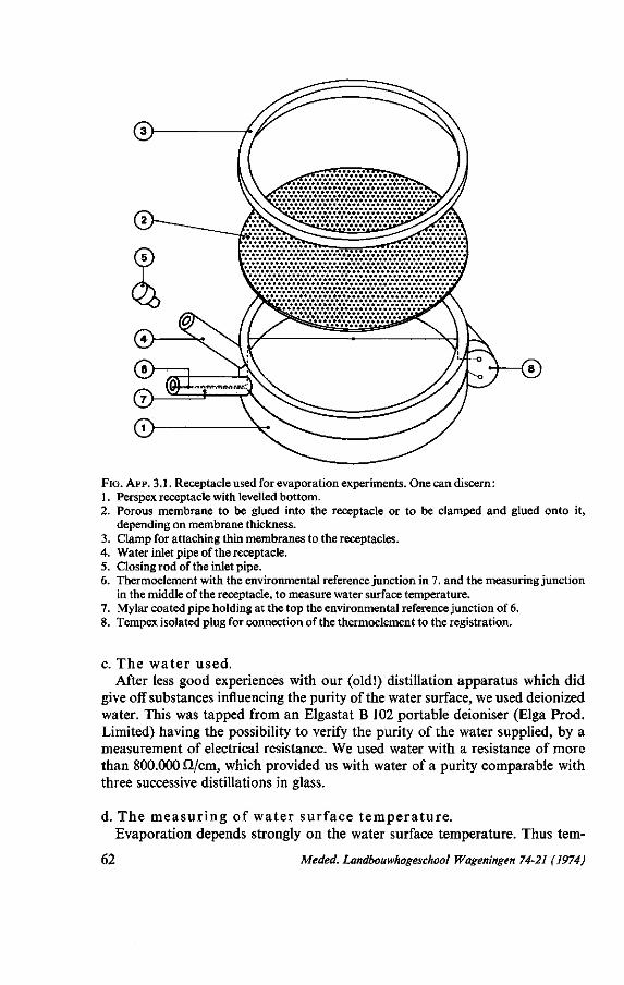
FIG. APP. 3.1. Receptacle used for evaporation experiments. One can discern: 1. Perspex receptacle with levelled bottom. 2. Porous membrane to be glued into the receptacle or to be clamped and glued onto it,

depending on membrane thickness. 3. Clamp for attaching thin membranes to the receptacles. 4. Water inlet pipe of the receptacle. 5. Closing rod of the inlet pipe. 6. Thermoelement with the environmental reference junction in 7. and the measuring junction

in the middle of the receptacle, to measure water surface temperature. 7. Mylar coated pipe holding at the top the environmental reference junction of 6. 8. Tempex isolated plug for connection of the thermoelement to the registration.

c. The water used. After less good experiences with our (old!) distillation apparatus which did

give off substances influencing the purity of the water surface, we used deionized water. This was tapped from an Elgastat B 102 portable deioniser (Elga Prod. Limited) having the possibility to verify the purity of the water supplied, by a measurement of electrical resistance. We used water with a resistance of more than 800.000 O/cm, which provided us with water of a purity comparable with three successive distillations in glass.

d. The measuring of water surface temperature. Evaporation depends strongly on the water surface temperature. Thus tem-


perature measurement of the water surface forms an important point. We started with observing the temperature difference between thermojuntions near (in) the evaporating surface and at deeper places. It is known that such differences are not too high. WARTENA (1959) for example found, in his temperature investigations in a class-A evaporation pan, that differences between surface and deeper layers were 0.1 °C at maximum. We found for our receptacle type, evaporating to a dry environment, the difference to be 0.3 °C at maximum for the lowest resistance type. Therefore measuring as near to the surface as possible was necessary. A second problem was that we wanted to measure with different water heights to be able to check experimentally any influence of air movement in the air below the membrane. This because of the fact that con-vectional contributions are strongly dependent on the thickness of the gas layer (Comp. SENGERS, 1965; STIGTER, 1966).

To be able to fulfill both requirements, measuring temperature near to the surface and changing water height, we constructed two receptacles for each type of membrane. One receptacle had a thermocouple with a junction in the middle of the metal wires stretched over the diameter of the receptacle, about 4 mm from the lower surface of the membranes (Fig. App. 3.1). The hot junction was at the top of a small tube of 3 cm long, attached to the receptacle and covered with Mylar (coated aluminium) for protection against the (low level) radiation. The wire ends terminated in an isolated plug which could be connected to the recording system outside the room. The second receptacle for each type of membrane was constructed without thermocouple and the water level could be freely chosen and could be permitted to become lower during subsequent measuring periods of 10 hours with only a weighing between such periods. (The lowering during one such a period being less than 1 mm, water level change can as a good approximation be taken linear with time).

We started our experiments with the receptacles provided with a thermocouple, having a junction in or near the water surface. From these measurements we calculated a first approximation of the boundary layer resistance of the air layer above the membranes as indicated below. Further we constructed a graph of surface temperature depression against total resistance (using the calculated values), going from 1.5°C at 13.5 s/cm to 4.1 °C at 4 s/cm. These values were now used and gradually improved during the measurements (where necessary) in which we worked at one and the same time with the two types of receptacle (for three different membranes). From the (improved) temperature against resistance curve we could now read the surface temperature of the receptacles without thermocouples, using the resistance calculations outlined below.

Calculations, measurements and results. The total diffusion resistance Rtot for water vapour diffusion from the water

surface inside the receptacle to the bulk chamber air is given by :

Rtot = Rr + Rm + Rb (22)


with as in (4)

Rm = Rend, 1 r Rpores T~ Rend, 2 (23)

In (22) i?r is the resistance to diffusion of the air layer from the water surface onwards up to the boundary of the lower end effect layer, Rm is the total membrane resistance, end effects included, and Rb is the resistance of the overall boundary layer above the membrane from the boundary of the upper end effect layer onwards.

Having the membranes mounted with the mouth end at the lower side, Renä,i is the end effect at this lower side. The isopsychres are here (and within the holes) different in form compared with the end effect Re„d,2 at the upper side, which was pictured schematically earlier (I, Fig. 3). The isopsychres have to depart with an angle of 90° from the walls. From the PENMAN/SCHOFIELD calculations used in the main text one finds (see Table App. 1.1) that the end effect at the conical side, Rend,i, should as a mean be taken as 75 % of the end effect of the nonconical side, Rend,2-

The thickness, m, of the layer in which the effective end effect Reni,2 takes place can be approximated by (Appendix 2 of PARLANGE and WAGGONER, 1970, their Fig. 1):

m = iz X i/8 (24)

with i the 'interstomatal' distance. For the effective layer in which Rendfl takes place we consequently use m' = 0.75 m.

We need to approximate a value for the thickness of the latter layer, because if the resistance Rr is taken from the water surface to the membrane surface onwards, as done in LEE'S experiments, this layer is figuring twice in the calculations. One time in the end effect calculation and one time (with a higher value) in Rr. We need to approximate the thickness of the layer in which Rend,2 occurs because of the fact that we will make use below of elimination of Rb by using an effective Rb not completely identical for different membranes. This inequality arises from the fact that the end effect layers protrude into the boundary layer as defined for a flat plate. This will be taken into account below. Omitting the two effects outlined above would result in errors between 3% (20 W) and 12% (125 P,R) in the final resistance values measured, which is just equal to or higher than the error limits given.

Our second improvement stems from the elimination of a second series of problems encountered in determining Rr + Rb. LEE used open receptacles to determine Rb + Rr. He took it for granted that the air within the receptacle above the water surface was absolutely in rest (so Rr identical) under a membrane and without a membrane, and he assumed air movement over the receptacles to be also identical under these two conditions (identical Rb). Now at least in one of LEE'S evaporation chambers air speed was higher than 1 m/s, in the other it seems at least unlikely that the air was completely at rest. We investigated the existence of air movement within an open receptacle indirectly


by having a 0.2 mm junction of a thermocouple in the water of a half filled receptacle. The other junction was held a few mm above the water surface. No artificial ventilation whatsoever was present in the chamber. The type of registration of this low time constant junction was clearly different when the receptacle was closed on top by a membrane in comparison with the situation when it was open. Air movement highly influenced the signal, fluctuating around the long term mean, in the latter case, being an indirect proof for the air in the open receptacle being not at rest. The registration for the closed receptacle was calm.

This information may be supplemented by the following reasoning regarding the air below the membrane. Free convection flow comes into existence only if there exists a certain angle between density gradients and the acceleration of gravity vector. The evaporating surface is in our case certainly cooler than the ambient air or membrane. So the air near the water surface is cooler, inducing a stable situation. This situation is of course different from the one described in the earlier mentioned paper by PENMAN and SCHOFIELD (1951), who argue that such density gradients, existing at a horizontal evaporating surface, do provoke marked air currents (Comp. (I), p. 20). In their case no side wall is present and horizontal air density gradients do exist at the edges of the surface. These gradients do make an angle with the vertical, and it is for that reason (and not from the vertical gradient) that air movement occurs.

The only situation to be regarded in our case is the evaporation inhomoge-neity at the wall of the receptacle, which may introduce temperature gradients in (and over) the water. Firstly the effect is partly compensated for by a small influence of surface tension forces, increasing the evaporating surface per unit of horizontal surface near the wall. Secondly the good thermal conductivity of the water will make the wall influence small. Moreover the influence of the effect becomes smaller the higher the surface/circumference ratio, which was the reason to use fairly large receptacles. On the ground of the above and being sure that air flow over the membrane did not influence air below the membrane it is also to be expected theoretically that the air under the membrane is at rest. Changing Rr (water level) during measurements with the same membrane did not influence in any systematic way the values measured for Rm. As the influence of convection has to be highly dependent on Rr this finally formed the experimental evidence that the method to calculate Rr from the (corrected) air layer thickness is sound in practice.

Regarding Rb LEE'S suppositions are doubtfull for the same reason (difference in air flow over an open and a closed receptacle) as given above. However, calculations for this resistance are not easy to make in low wind speeds (Comp. (I), p. 20, 21). One might suggest to enhance air movement in the room to lower the influence of Rb, but enhancing air flow increases intollerably spatial in-homogeneity of air flow in the chamber. This makes comparison of Rb over different receptacles, for the sake of elimination, impossible.

We solved the problem by using at all measurements for the determination of Rb alternately one or two of four receptacles closed at the top by membranes

Meded. Landbouwhogeschool Wageningen 74-21 (1974) 6 5

with very low resistances, ranging from 0.3 to 0.5 s/cm (125 P, 125 R, 100 R, 125 T). These membrane resistances were originally calculated by the PENMAN

and SCHOFIELD formula. Even in the case that the approximation should have been in error by 20 %, the absolute error would have been less than 0.1 s/cm. This may be compared with the mean value of Rb, 3 s/cm, calculated from (22) using

Rtot = àe/I (25)

The Ae value is the difference between the saturated vapour concentration at surface temperature concerned and the ambient air vapour concentration in the chamber. The quantity I is the vapour loss per unit of time and surface measured by weighing. Rtot was for these low resistance receptacles found to range from 5 s/cm to 9 s/cm (depending on Rr), yielding a mean value for Rb in the neighbourhood of 3 s/cm. This value indicated that the air movement over the receptacles was very low (Comp. I, p. 20). Values at different places of the leveled surface over which the receptacles were distributed yielded no systematical differences, indicating mean homogeneity of air flow over the periods of measurement.

Before applying now the value found for Rb over the low resistance membranes to the evaporation measurements with the other membranes, taking/?,, over all membranes to be almost identical, we have to make still one small correction, as already indicated above. The real boundary layer over a flat plate, in the form of our receptacle upper surface, can be interpreted, for each type of air flow over it, as a layer of stagnant air of a certain mean thickness, taking edge effects into account in the value of this mean (I, p. 11, 13). This layer will be the same over a plate with holes if no roughness elements increase the turbulence of air flow. This again means that the end effects of the membranes do occupy a different part of this layer, which part is again figuring twice in the calculations if not corrected for. The calculation of an effective Rb (I, p. 12, 13) over each membrane is done, using (24), from :

meff " mref Rb = Rb, eff = Rb, ref yj (26)

in wich equation Rb,ref is the boundary layer value measured above the low resistance receptacles and mref and meff are the thicknesses of the air layers above the low resistance receptacles and the other receptacles concerned respectively. In practice meff and mref do not differ more than 0.6 mm.

Knowing the effective Rb, the unknown membrane resistances follow from (25), (22) and (23). During the measurements either one receptacle with unknown membrane resistance was placed on the table between two of the four receptacles with known low resistances (early in the investigations to crosscheck results with different known membranes at different places) either one receptacle with a known resistance was placed between two receptacles with membranes to be measured. Opposite to each type provided with a thermocouple a receptacle of the same type (with the same membrane) without a thermocouple


TABLE APP. 3.1. Results of the measurements of unknown membranes with the improved evaporation method. Error limits given are estimated from the deviations of the averages.

80 T

0.6 s/cm 0.7 0.6 0.4 0.4 0.7 0.6 0.7 0.3 0.4

0.55±0.15

15 S

2.5 2.9 3.1 3.0 3.2 2.5 2.7 2.5 2.4 2.5

2.75 ±0.25

100 T

0.5 0.8 0.5 0.8 1.2 1.0 0.9 0.8 0.7 0.8

0.80±0.15

20 T

5.2 5.0 5.0 4.8 4.9 4.9 5.0 4.9 4.9 4.9

4.95±0.10

30 R

1.2 1.5 1.2 1.7 1.7 1.4 1.3 1.5 1.3 1.4

1.40±0.15

15 T

5.3 5.4 5.4 5.5 6.1 5.6 5.6 5.3 5.3 5.4

5.50±0.15

40 T

2.5 2.3 2.4 2.3 2.5 2.5 2.3 2.4 1.9 2.1

2.30±0.15

20 T-VERO

5.7 5.8 5.9 5.8 5.8 5.9 5.7 5.9 5.9 5.7

5.80±0.10

30 T

2.6 2.9 2.6 3.2 3.1 2.7 2.6 2.7 2.4 2.3

2.70±0.20

20 W

9.9 10.5 9.9

10.0 9.8

10.3 9.9 9.9

10.0±0.20

was placed. The latter were brought one by one within the Mettler B5-mg balance next to the levelled surface. This was repeated after each of 3 to 5 periods of about 10 hours. At the beginning of each new period some water was supplied to the receptacles holding the thermocouples to keep the junction in or just below the surface. As indicated earlier, the temperatures were continuously measured, to incorporate the influence of low trend changes in the environmental conditions, introducing for example small deviations from the resistance/surface temperature depression diagram constructed. Each membrane (except accidentally 20 W) was tested over 10 periods as mentioned, the accuracy being ± 0.3 to 0.5 s/cm, for each individual measurement, depending among other things on the value of Rlot. Results are given in Table App. 3.1.

After having proved the factual non-existence of convection influence it is not longer necessary to work with the two-receptacles method with the thermocouple as near to the lower membrane surface as compatible with the experiment and as near to the water surface as possible. A method with closed receptacles with a thermojunction at about half its height, filled up in the beginning to for example 1 cm above the junction, may be used in the future.


Correction has to be made for small differences in temperature between surface and deeper layers but this can be done without much trouble. Especially for diffusion resistances to which calculations such as the PENMAN/SCHOFIELD calculations do not easily apply, such a method will yield excellent results.


11. APPENDIX 4

A CHECK ON INFLUENCES OF THE TEMPERATURE MEASURING SYSTEM IN

GROWTH CHAMBER EXPERIMENTS ON LEAVES

A first series of experiments was done in a growth room of the Institute for Biological and Chemical research on Field Crops and Herbage (I.B.S.), on an artificial leaf as described in the main text (but without a thermocouple) and on bean leaves (Phaseolus Vulgaris). The latter ones in combination with an other experiment on these leaves (H. LOF, unpubl. results). The day before and after the measuring day we yielded an Rp of 1.85 ± 0 . 1 s/cm in the way indicated in (II) and Chapter 2 of this article. Measurements on the wet artificial leaf, with R, = 0, yielded Rp = 1.70 ± 0.05 s/cm (Table App. 4.1). A repetition in a second and third series of experiments on a wet artificial leaf, in a laboratory environment, revealed again a difference of 0.15 and 0.10 respectively between the lower Rp measured on these wet leaves and the calibrated Rp. An important observation related to this question was that the effect was not significant (difference 0.05 s/cm) in series of measurements on wet filter paper on our calibration heating source (II, Fig. 6). Such measurements were for example made in the same series as reported in Table 2.

Although the error limits touch each other it is of interest to look for existing sources of systematical errors. Differences between the situation at the heating source and at the artificial leaves may be found either in factors regarding the temperature indication or in the fact that the instrument is in different clamps during calibration and measuring (II, Fig. 3-8).

During calibration the rubber sealing fringe is just touching the surface, the clamp being put on the filter paper. During the measurements reported in Table App. 4.1, the sensor chamber is in its field clamp (this article Fig. 5). Now in a special experiment we exerted pressure on the calibration clamp, apart from the weight normally used on top (e.g. II, Fig. 6). We found the transient times becoming shorter, so Rp becoming smaller. The same phenomenon we observed when exerting extra pressure on the field clamp on the artificial leaf, bringing the difference in Rp even to 0.2 s/cm. Therefore an explanation of lower Rp as measured on the artificial leaf has to be sought in water at the rubber sealing fringe, coming out of the filter paper by the normal clamp force. This could be confirmed visually. It increases the effective evaporating surface and shortens the diffusion path.

Regarding the supposed absence of influence of temperature factors one may state : 1) The thermistor and the thermoelement have been calibrated against each

other. Therefore differences between them can not explain systematical errors. 2) The important existence of a near equilibrium temperature situation of the

leaf, over the measuring period of the short transient times, was checked by


also calculating the i?p-values from calibration and measurement via the long transient times (II, p. 22, 23). The differences between Rps found in this way remained the same, which is a direct indication for sufficient temperature equilibrium over this short transient time period. 3) The equilibrium temperature of the leaf indicated by the thermistor in equi

librium with the leaf must have been the correct one. This may be shown taking into account our observations at the artificial leaf and eventual gradients to be expected over the measured leaf parts not touched by the copper slice.

As may be observed from Table App. 4.1, measurements on wetted bean leaves yielded a resistance of even 1.6 ± 0.1 s/cm and measurements on bean leaves from which the epidermis was roughly scoured away did give the same result. Again it could be proved that with the short transient times involved (ca. 7 seconds) the time constant was, also on these natural leaves, short enough to produce temperature equilibrium over the short measuring period. Short and long transient times yielded the same results.

Two effects can be mentioned that are influencing at the real leaves Rp in comparison to its value measured at a smooth filter paper surface at the heat sink. Both effects increase the effective evaporating surface.

Firstly the natural surface of a leaf is rarely as flat as a free water surface. Therefore wetting or scouring this natural surface will increase S in (see II, eq. 4):

4 , = | w + ^ i „ j ^ (27)

compared with the free water surface measurement on heat sink filter paper. So Rp becomes lower if we use the porometer opening, 2 cm2, for S. Assessing the effect quantitatively is more difficult but an effect of 10% seems far within the existing possibilities. Such an effect of course forms no error under dry surface conditions as long as it is representing in a natural way a leaf area of

TABLE APP. 4.1. /{„-measurements on wet artificial leaves and bean leaves with a calibrated Äp-valueof 1.85 ± 0.1 s/cm.

Wet artificial leaf

1.70 1.71 1.69 1.69

1.70±0.05

Wetted bean leaves

1.60 1.57 1.49 1.78 1.72 1.62

1.6±0.1

Scoured bean leaves

1.51 1.75 1.46 1.46 1.70 1.56 1.79 1.55

1.6±0.1


2 cm2. We will only be in error in the case that clamping the device onto the leaf deforms the surface.

Secondly of course a good contact between leaf and temperature measuring system, induced by exerting slight pressure on the measured leaf part, runs somewhat counter to the requirement of a completely undeformed surface. It was observed visually that for the rigid artificial leaf this deformation, increasing the area evaporating into the sensor chamber (and shortening somewhat the mean diffusion path) did not take place. The same applies to the rigid corn leaves. With the bean leaves, which surfaces are more easily transformable, such visual observations were more difficult to make, but there was no indication for an appreciable effect. Only the impression of the thermistor was always visible here at the side measured by the porometer. The error was estimated, however, to be only in the neighbourhood of 2 to 3 %.


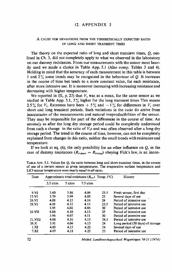
12. APPENDIX 5

A CAUSE FOR DEVIATIONS FROM THE THEORETICALLY EXPECTED RATIO

OF LONG AND SHORT TRANSIENT TIMES

The theory on the expected ratio of long and short transient times, Q, outlined in Ch. 3, did not completely apply to what we observed in the laboratory on our dummy resistances. From our measurements with the sensor most heavily used we made a choice in Table App. 5.1 (Also comp. Tables 3 and 4). Holding in mind that the accuracy of each measurement in this table is between 1 and 2 % some trends may be recognized in the behaviour of Q. It increases in the course of time but tends to a more constant value, for each resistance, after more intensive use. It is moreover increasing with increasing resistance and decreasing with higher temperature.

We reported in (II, p. 23) that Vs was as a mean, for the same sensor as we studied in Table App. 5.1, 3% higher for the long transient times This means 2.5% for Vt. Extremes have been + 5% and —1 % for differences in Vt over short and long transient periods. Such variations in the ratio do arrive from inaccuracies of the measurements and natural irreproducibilities of the sensor. They may be responsible for part of the differences in the course of time. An anomaly as after the long dry storage period could be completely understood from such a change in the ratio of Vts and was often observed after a long dry storage period. The trend in the course of time, however, can not be completely explained from changes in this ratio, neither the small trends with resistance and temperature.

If we look at eq. (6), the only possibility for an other influence on Q, in the case of dummy resistances (Ri,short = Ri,iong) obeying Fick's law, is an incon-

TABLE A P P . 5.1. Values for Q, the ratio between long and short transient times, in the course of use of a certain sensor at given temperatures. The evaporative surface temperature and LiCl-sensor temperature were nearly equal in all cases.

Date

9.VI 13.VI 26.VI 28.VI

24.VII

21 .VIII 26.X

l .XI 7.XI

Approximate

2.5 s/cm

3.60 3.79 4.08 4.08 3.95 4.04 3.96 4.08 3.91 4.05 4.07

: total resistance (Rtùt

5 s/cm

3.88 3.99 4.13 4.12 4.02 4.10 4.07 4.10 4.04 4.15 4.18

7.5 s/cm

4.04 4.05 4.16 4.13 4.06 4.13 4.11 4.15 4.13 4.22 4.25

) Temp. (°C) History

23.5 23 24 23.5 30 25 30 24.5 24 24 23

Fresh sensor, first day Several days of use Period of intensive use Period of intensive use Period of intensive use Period of intensive use Period of intensive use Period of intensive use Long period (50 days) of storage Several days of use Period of intensive use


sistency in Rp. We reported in (II, p. 25) that as a mean a lower R„ was found for the long transient times, differing about 0.1 s/cm from the corrected mean value of the short periods (1.8 s/cm). Now from Table App. 5.1 one gets the impression that the change in Q is becoming smaller at higher resistances. This is confirmed by the example of Qmean in Table 3, pictured in Fig. App. 5.1. If we add that for the mean of this measurement the V, was about 4 % higher for longer transient times compared with the short ones, Q calculated via (6) and (7) becomes about 4.30 for Rt > Rp. This is in accordance, within the possible accuracies, with Fig. App. 5.1. It suggests indeed an influence of R„ on Q, as in (6) for dummy resistances i?j,i0„9 = Ri,sh0rf RP must be higher for the denominator in (6) than for the numerator. The influence of a higher Rp diminishes as Rt

increases. The above yields a slight deviation from the theory that Rp can be calculated definitely, under all circumstances, from equilibrium transport processes only (II, Ch. 5).

A difference between Rps of short and long transient times might be explained from a not complete obeying to Fick's law. The acceptance of full obeyance to this law formed the basis for the derivation of (27) and (6). We suggest here that we are meeting consequences from the fact that adding the two volumes Vs and Vp is not fully permitted in and just after the starting up period. Between the porometer volume and the sensor volume we have the small diffusion resistance of the boundary layer surrounding the sensor (II, Ch. 5). This means that there is a delay between the concentration changes taking place in

4.30

4.25

(.20

1.05

£.00

3.95 10 11 12 13 14 15 • Rtot

FIG. APP. 5.1. Change of Qmea„ of Table 3 with R,ot ( = R, + Rp) in s/cm.


Vs and in Vp. It lowers, notably in the first part of the dynamical process, the apparent change of concentration in Vs compared with the situation that this apparent concentration change should take place completely simultaneously with the change in Vp. This effect is found back in higher short transient times. The situation is comparible with a second order system reaction on a step function entrance concentration change. Therefore the effect is also higher when Vs

is more comparable in value with Vp. For high Vs the lead in Vp becomes negligible relative to the time scale of the processes taking place in Vs.

It is clear that the effect on the long transient times may be expected to be about a quarter of the effect on the short transient times. For the influence of the effect on Q, via (6), of say at maximum about 12 % for the total resistance of 2.5 s/cm, we must therefore countwith a 16% influence on (&t)short and a 4% influence on (A?),0„9 by the same effect. This means, however, that the maximum error for the long transient times will be only 0.1 s/cm in Rp, and by the way normally much lower than the error limits involved. As a consequence Fig. App. 5.1 pictures the effect on short transient times mainly.

It is surprising, at first glance, that we measured, also for very fresh sensors with low Vt, that Rp was different for short and long transient times, without influencing Vt. We found even differences of at maximum ca. 0.3 s/cm, Vt remaining constant within the limits given earlier. We have here, however, again to do with the sensor property described earlier (II, p. 23, 24). Vt remains under all conditions independent of the rate of change of external concentrations.


13. APPENDIX 6

A GUIDE TO USERS OF POROMETERS

It is useful to draw from the experience gained in the research described in this publication and the foregoing ones a certain set of rules, with all proper reserve, for users of porometers. One has to hold in mind that these rules are checked to be valid on small Hygrodynamics LiCl-sensors and that some of them may be different for other sensors, either LiCl-ones or other types.

1) One should use a porometer chamber as simple as possible but with suppression of convectional influences and with an easy access of the entering

water vapour to the total sensor surface.

2) Drying of the porometer air should be done with the least possibility of entering of hygroscopic dust, but supply of fresh C 0 2 should be possible

if consumption of porometer-C02 is expected.

3) Construction materials should be used which have as low water absorption and adsorption as the polypropylene or the teflon tested by us.

4) Flat thin perforated membranes, from materials with low water absorption and adsorption, with not too complicated types of holes, should be used for

calibration purposes. A choice should preferably, although not necessarily, be made in accordance with the expected values of the resistances to be measured. Mutual influence of neighbouring pores should be avoided.

5) A waiting time, depending in principle on the drying speed and the time constant of the sensor, should be applied prior to any measurement. During

this time the sensor should be held at a fixed indication of electrical resistance, to be used in all following measurements as a starting point.

6) It might be useful, to promote easy handling of results, to do some dummy calibrations after very long dry storage periods, as anomalies have been ob

served directly after such periods.

7) For calibration purposes at each sensor temperature the values of a volume Vt and a porometer resistance Rp should be determined. One should use the

solution of the equation for the change of water vapour concentration with time in the apparent calibration volume Vt. This should be done using two or more calibration membranes, depending on the accuracies with which the true membrane resistances are known, of which one may be zero(i?,=0).

8) Calibration can be done for one transient time between two fixed electrical sensor resistances either for two (or even more) transient times. This depends

on whether a check on stomatal behaviour during the measurements, on the temperature measuring system or on stress phenomena is wanted.

Meded, Landbouwhogeschool Wageningen 74-21 (1974) 7 5

9) In the case of two transient times, for using their ratio in forecasting, a check should be made on the behaviour of this ratio up till the limit determined

theoretically from the equations mentioned in 7). For this purpose a relatively high resistance membrane should be used.

10) The definite choice made for the fixed starting point of the starting up period may depend on an experienced Vt of the sensor. It is recommended

to prevent too high an influence of a starting up effect and to prevent too short transient times in relation to the time constant of the temperature measuring system.

11) The fixed electrical resistance to be passed as a lower limit should be preferably, although not necessarily, at the bottom of the log-linear sensor

calibration diagram. The upper limit should still be on the log-linear part of the diagram. The choice of the latter depends on the used opening, S, in relation to permitted clamping times. The values of V, and i?,, the resistances to be measured, can also be taken into consideration.

12) The ratio of long and short transient times, if using this modification of the method, will lay preferably between 3 and 5. This determines the con

ditioning of the second and third electrical resistance points serving as limits. Again such limits can be changed depending on the fact whether relatively high or low diffusion resistances will have to be measured, whether a large or small S is used and whether V, is large or small.

13) The same values as found for Vt and Rp in calibrations with fixed starting points and limits should be used for (field) measurements. This should be

done either averaged for the day before and the day after a measuring day or determined on the measuring day itself, directly prior to the measurements concerned.

14) The behaviour of the temperature dependence of Vt should be checked occasionally in a special calibration series.

15) The only case in which a sensor should no longer be used is in the case that momentaneous reproducibility under fixed conditions does no longer

occur.

16) When not in use sensors and porometers should be stored over silica gel and be transported in containers holding silica gel.

17) The field temperature measuring system should be built in a way that the necessary equilibrium leaf temperature over the (short) transient times is

at least indicated by the temperature sensor after that time. Influence on the natural effective evaporating surface must be prevented.


leaf diffusion resistance to water vapour and its …

Documents