leaning against the wind when credit bites back - ijcb · leaning against the wind when credit...

Leaning Against the Wind WhenCredit Bites Back∗

Karsten R. Gerdrup, Frank Hansen,Tord Krogh, and Junior Maih

Norges Bank

This paper analyzes the cost-benefit trade-off of leaningagainst the wind (LAW) in monetary policy. Our starting pointis a New Keynesian regime-switching model where the econ-omy can be in a normal state or in a crisis state. The setupenables us to weigh benefits against costs for different system-atic LAW policies. We find that the benefits of LAW in termsof a lower frequency of severe financial recessions exceed costsin terms of higher volatility in normal times when the severityof a crisis is endogenous (when “credit bites back”). Our qual-itative results are robust to alternative specifications for theprobability of a crisis. Our results hinge on the endogeneity ofcrisis severity. When the severity of a crisis is exogenous, wefind that, if anything, it is optimal to lean with the wind.

JEL Codes: E12, E52, G01.

1. Introduction

Since the global financial crisis, attention has been devoted to poli-cies that promote financial stability. Empirical literature has foundthat periods of high credit growth can lead to deeper and more

∗This paper should not be reported as representing the views of Norges Bank.The views expressed are those of the authors and do not necessarily reflect thoseof Norges Bank. The paper was presented at the Riksbank-BIS Workshop “Inte-grating Financial Stability into Monetary Policy Decision-making—The Model-ling Challenges,” November 2015; the Annual International Journal of CentralBanking Research Conference at the Federal Reserve Bank of San Francisco,November 2016; and at various seminars and workshops in Norges Bank. Weare grateful to the participants at the various seminars and workshops, andLars Svensson, Carl Walsh, Mikael Juselius, Ragna Alstadheim, Andrew Filardo,Phurichai Rungcharoenkitkul, Leif Brubakk, Drago Bergholt, Steinar Holden,Helle Snellingen, and Veronica Harrington for useful comments.

287

288 International Journal of Central Banking September 2017

protracted recessions, i.e., “credit bites back” (Jorda, Schularick,and Taylor 2013). Macroprudential policy measures have been intro-duced in many countries to prevent and mitigate systemic risksrelated to high growth in credit and asset prices, and can be con-sidered the first line of defense against financial instability sincesuch tools can be both more granular and targeted to the sourceof risk. However, there is great uncertainty regarding the effective-ness of macroprudential policy tools and the appropriateness of legalframeworks. Monetary policy can still play a powerful role by “lean-ing against the wind” (LAW), as it is transmitted more broadly toall sectors in the economy and also to shadow banks1; see Smets(2014) for a broader discussion.

Financial crises are rare events and have historically occurredevery fifteen to twenty years on average; see Taylor (2015). LAWpolicies can potentially lead to a loss of central bank credibility sincesuch events are hard to predict. Justifying tight monetary policy canbe difficult since we cannot observe the possible gains in terms ofa lower frequency and severity of crises. If interest rates are sys-tematically kept higher than those implied by price stability, infla-tion expectations can fall and the inflation-targeting regime couldlose credibility. Many authors have furthermore shown that withlong-term debt contracts, raising monetary policy rates to reducethe credit-to-GDP level can have perverse effects since GDP growthfalls faster and stronger than credit; see Svensson (2014) and Gelain,Lansing, and Natvik (2015). However, gains can be high if leaningagainst excessive financial stability risks can reduce the probabil-ity and severity of crises longer down the road. The recent finan-cial crisis showed that monetary policy, or economic policy in gen-eral, has limitations when it comes to cleaning up after a crisis hasoccurred.

This paper will investigate to what extent monetary policyshould react to financial stability risks and deviate from the pol-icy it would have chosen in the absence of such risks. The ques-tion of LAW is only relevant insofar as financial stability risk and

1Or “it gets in all of the cracks,” as Jeremy Stein put it in a speech at the“Restoring Household Financial Stability after the Great Recession: Why House-hold Balance Sheets Matter,” a research symposium sponsored by the FederalReserve Bank of St. Louis, February 7, 2013.

Vol. 13 No. 3 Leaning Against the Wind 289

inflation are not perfectly correlated. Negative shocks to inflationmay give rise to a trade-off in monetary policy because bringinginflation back to target may have to be achieved at the expense ofa buildup of financial imbalances. Small open economies are facedwith such trade-offs when international interest rates fall, and thecentral bank has to reduce domestic interest rates to reduce thedegree of currency appreciation and lower imported inflation. Theopen-economy dimension also gives rise to a trade-off between sta-bilizing inflation and output when the economy is hit by a shock toaggregate demand (no divine coincidence between stabilizing infla-tion and output). This means that a central bank cannot clean upafter a crisis has erupted by reducing interest rates without payingattention to inflation. For the setup to be relevant for small openeconomies, we use the estimated model of Justiniano and Preston(2010a) as the core model.

In our framework, LAW is motivated by agents underestimat-ing financial stability risks. When aggregate credit is accumulatedin the economy, agents do not incorporate the risk this poses toeconomic developments. We introduce regime switching into an oth-erwise standard open-economy New Keynesian model. This proce-dure enables us to analyze economic developments for an economythat occasionally experiences financial headwinds using a relativelyparsimonious model. While the financial system and its interactionwith economic developments is extremely complex, we simplify themechanisms to highlight some important policy trade-offs. We modelcredit developments as a separate block “outside” the core model.Credit, which will serve as a proxy for financial imbalances in themodel, only affects the probability of a crisis and the severity of acrisis and does not affect economic developments in normal times.Parameters controlling the probability of crises and the severityof financial recessions are calibrated based on a sample of OECDcountries.

When the economy makes the transition from a normal regimeto a crisis regime, aggregate demand is reduced abruptly. The mech-anisms behind this aggregate demand shock can be numerous. InCurdia and Woodford (2009, 2010) and Woodford (2012) a similarterm can be interpreted as credit spreads, the difference in equilib-rium yield between long-term bonds issued by risky private borrow-ers and those issued by the government. Higher credit spreads make


financial conditions worse for borrowers, reducing overall welfare.Aggregate demand can also fall as a result of strained balance sheets.When leverage is high, households, non-financial companies, andfinancial institutions are at higher risk of defaulting. When agentstry to de-lever, assets may be sold at fire-sale prices, creating debt-deflation type spirals; see, e.g., Lorenzoni (2008), Bianchi (2011),and Bianchi and Mendoza (2013). Consumers reduce consumptionin order to strengthen their balance sheets; see Mian and Sufi (2011)and Dynan (2012). The underlying idea is the same as in Woodford(2012):

The idea of the positive dependence on leverage is that themore highly levered financial institutions are, the smaller theunexpected decline in asset values required to tip institutionsinto insolvency—or into a situation where there may be doubtsabout their solvency—and hence the smaller the exogenousshock required to trigger a crisis. Given some distribution func-tion for the exogenous shocks, the lower the threshold for ashock to trigger a crisis, the larger the probability that a crisiswill occur over a given time interval.

This paper is close in spirit to Ajello et al. (2015). They study theintertemporal trade-off between stabilizing current real activity andinflation in normal times and mitigating the possibility of a futurefinancial crisis within a simple New Keynesian model with two statesand an endogenously time-varying crisis probability. While they usea two-period setup, we use an infinite time horizon. Using a longerhorizon can reduce the benefits of leaning, since credit growth even-tually picks up after a monetary policy tightening aimed at miti-gating financial stability risk. This point has been highlighted bySvensson (2016) and reflects that real credit, which determines theprobability of a crisis, is assumed to return to a specific steady-statelevel in his application. We calibrate the effect of an interest rateincrease on credit growth to reflect SVAR evidence for Norway. LikeAjello et al. (2015), we assume that the crisis probability is a func-tion of credit growth over a five-year period. We follow Alpandaand Ueberfeldt (2016), Pescatori and Laseen (2016), and Svensson(2016) in assuming that a crisis can occur at any point in time.Unlike Ajello et al. (2015) and Alpanda and Ueberfeldt (2016), weassume that the crisis severity is endogenous. This will increase the


benefit of leaning in monetary policy. Similar to Ajello et al. (2015),we will assume that private agents underestimate the probability ofa crisis. This is in contrast to Alpanda and Ueberfeldt (2016), whereagents are rational and perceive aggregate risks correctly, but nottheir own contribution to that risk.

We contribute to the literature by investigating systematic LAWpolicies. We find that the benefits of LAW in terms of a lower fre-quency of severe financial recessions exceed costs in terms of highervolatility in normal times when the severity of crisis is endogenous(when “credit bites back”). The LAW policy can be implementedby responding relatively more to fluctuations in output and/or byresponding directly to household credit growth. Compared with apolicy that does not take into account that a crisis can happen, a“benign neglect” policy, the LAW policy contributes to a lower lossand reduced tail risk in the economy. The costs are paid in termsof higher inflation volatility. Our qualitative results are robust toalternative calibrations of the probability of crisis. If, however, theseverity of crisis is exogenous, or the effect of credit on crisis severityis very small, the optimal response is to lean with the wind. Thisnests the results found in the literature, e.g., Ajello et al. (2015),Alpanda and Ueberfeldt (2016), Pescatori and Laseen (2016), andSvensson (2016), who find no (or very small) net benefits of LAWpolicies, and typically assume either no or a very small effect fromcredit to crisis severity.

The rest of the paper is organized as follows. We begin by estab-lishing empirical evidence to inform us about the link between creditand crisis probability and severity in section 2. This is used whenwe set up a model for analyzing LAW (section 3) and calibratingit (section 4). In section 5 we present some properties of the cali-brated model, while the results of our LAW analysis are in section6. We end with a section on sensitivity (section 7) and conclusions(section 8).

2. Can LAW Policies Make Sense?

We interpret LAW as monetary policy adjustments where the cen-tral bank reacts to financial stability risks and deviates from thepolicy it would have chosen in the absence of such risks. Two centralassumptions must be fulfilled for LAW to be able to bring benefits.


Table 1. Estimated Effects of a Monetary Policy Shock onReal Credit in VAR Studies

Peak Effect ofPaper Country MP Shock (%)

Goodhart and Hofmann (2008)a Panel Approx. −1.25Assenmacher-Wesche and Gerlach (2008)b Panel Approx. −0.8Musso, Neri, and Stracca (2011)c US Approx. −3Musso, Neri, and Stracca (2011)c EA Approx. −2Laseen and Strid (2013)c SWE Approx. −0.8Robstad (2014)c NOR Approx. −0.8Pescatori and Laseen (2016)c CAN Approx. −0.8

aBased on bank loans to the private sector.bBased on total loans to private non-bank residents.cBased on credit to households.

First, monetary policy must be able to affect the relevant financialvariables. Second, financial crises cannot be purely exogenous events.The probability of a crisis and/or the severity of a crisis must belinked to financial imbalances. In this section, we evaluate to whatextent these necessary conditions are fulfilled, both based on theexisting empirical literature and estimates based on a sample oftwenty OECD countries. In our setup, we use the five-year growthrate in real household credit as a measure of financial imbalances(similar to, e.g., Ajello et al. 2015).

2.1 The Effect of Monetary Policy on Credit

The empirical literature has established a clear link from monetarypolicy to credit. Table 1 provides an overview of VAR estimates ofthe peak effect on the level of real credit following a 1 percentagepoint increase in the nominal interest rate.

The peak effect of monetary policy on real credit is similar inmagnitude across the different studies. This indicates that mone-tary policy may play a role in affecting credit developments. Papersfocusing on (small) open economies (e.g., Laseen and Strid 2013,Robstad 2014, and Pescatori and Laseen 2016) suggest that the peakeffect on real household credit following a monetary policy shock that


raises the nominal interest rate by 1 percentage point is around 0.8percent. The effect is estimated to be larger when considering theUnited States or the euro area as a whole (Musso, Neri, and Stracca2011). In our paper, we will make use of the estimates in Robstad(2014), which are in the lower end of the estimates.

2.2 The Effect of Credit on the Probability of a Crisis

There is a general consensus in the literature that excessive creditaccumulation is one of the main drivers of financial crisis (see, e.g.,Reinhart and Rogoff 2008, Schularick and Taylor 2012, Anundsen etal. 2016, and Jorda, Schularick, and Taylor 2016). We estimate theprobability of a crisis based on a panel of twenty OECD countriesover the period 1975:Q1–2014:Q2.2 These are the same data used inAnundsen et al. (2016). In contrast to Anundsen et al. (2016), whoestimate the probability of being in a pre-crisis period, we reformu-late the model and estimate the probability of a crisis start directly(similar to, e.g., Schularick and Taylor 2012). Our dependent vari-able takes the value of 1 if there was a crisis start in country i atquarter t and zero otherwise.3 The probability of a crisis start isassumed to depend on the five-year growth in real household credit(L). Using the logit specification, the probability of a crisis start incountry i in quarter t is given by

pi,t =exp(μi + μLLi,t)

1 + exp(μi + μLLi,t), (1)

where μi are country fixed effects and μL is the coefficient on thecumulative credit growth. The estimates we get are shown in table 2.

The estimates suggest that the steady-state (annual) probabilityof a crisis is approximately 3.3 percent. Further, there is a posi-tive effect of credit growth on the probability of a crisis. A plot ofthe estimated logit function as a function of cumulative real creditgrowth can be found in figure 8.

2Countries included are Australia, Austria, Belgium, Canada, Denmark, Fin-land, France, Germany, Greece, Italy, Japan, Korea, Netherlands, Norway, Por-tugal, Spain, Sweden, Switzerland, the United Kingdom, and the United States.

3To avoid post-crisis biases, as discussed in, e.g., Bussiere and Fratzscher(2006), we omit observations for when a given country was in a crisis.


Table 2. Estimated Parameters in the Logit Model

(1)

Five-Year Real Credit Growth 2.232∗∗

(1.099)Constant −4.792∗∗∗

(1.026)Country Fixed Effects Yes

Pseudo R-Squared 0.0424AUROC 0.725Observations 1,832

Note: Clustered standard errors are reported in parentheses below the point esti-mates, and the asterisks denote significance levels: ∗ = 10 percent, ∗∗ = 5 percent,and ∗∗∗ = 1 percent.

2.3 The Effect of Credit on the Severity of a Crisis

The empirical literature has found that credit accumulation in aboom is important for economic activity during the bust (see, e.g.,Jorda, Schularick, and Taylor 2013, 2016 and Hansen and Torstensen2016). In our framework we are interested in how credit accumula-tion in the boom affects the path for the output gap during busts.To this end, we use local projection methods (Jorda 2005) to esti-mate how the five-year growth in real household credit affects thepath for the unemployment rate during a financial crisis. We add theunemployment rate to the data used in Anundsen et al. (2016).4 Tokeep things simple, we estimate paths only for the unemploymentrate during financial recessions (defined as recessions that coincidewith a financial crisis within a two-year window).5 The correspond-ing effects on the output gap are then calculated based on Okun’slaw.

4Data on unemployment rates were gathered from FRED (Federal ReserveEconomic Data). To get as long quarterly series on unemployment rates as possi-ble, the definition of the unemployment rate differs somewhat between countries.For some countries, registered unemployment was used; for others, we have usedharmonized rates. Some include the entire population, while some include onlythe working-age population.

5Recession dates are based on Hansen and Torstensen (2016).


Figure 1. Change in Unemployment Rate from the Startof the Crisis (percentage points)

0 2 4 6 8 10 12 14 160

1

2

3

4

5

6

Number of quarters from start of crisis

Per

cent

age

poin

ts

Pre−crisis debt growth on averagePre−crisis debt growth 1 standard deviation higher

Notes: The solid line is the path for the unemployment rate conditional on thefive-year growth in household real credit at the peak of financial recessions. Thedashed line illustrates the path when the five-year growth in real household creditis one standard deviation higher at the peak.

Figure 1 and table 3 show the local projection results for theunemployment rate during a financial crisis conditional on pre-crisiscumulative credit growth. In figure 1, the solid black line shows theincrease in unemployment during a financial crisis conditional on theaverage five-year growth in real credit at the peak of the cycle. Thedashed line shows the corresponding path for the unemployment ratewhen the five-year growth in household real credit is one standarddeviation higher at the peak.6 The increase in the unemploymentrate during a crisis is both higher and more protracted in this case.The difference between the two paths is also significant; see table3. Our results are in line with the results in Jorda, Schularick, andTaylor (2013) and suggest that “credit bites back.”7

6The average cumulative growth in real household credit at the peak is 11percent in the data. The standard deviation is about 17 percent.

7The magnitude of this effect is, naturally, uncertain. Estimates may differdepending on the number of countries analyzed, the sample period, and the empir-ical approach used. For example, Jorda, Schularick, and Taylor (2016) documentthat the buildup of mortgage credit in the boom has become more important forreal economic activity during recessions post–World War II.


Tab

le3.

Loca

lP

roje

ctio

nfo

rth

eU

nem

plo

ym

ent

Rat

eduri

ng

Fin

anci

alC

rise

s

Hor

izon

(1)

(2)

(3)

(4)

(5)

(6)

(7)

(8)

Con

stan

t0.

00.

30.

71.

12.

5∗∗

3.5∗

∗∗3.

8∗∗∗

4.1∗

∗∗

(0.2

)(0

.3)

(0.5

)(0

.8)

(1.0

)(0

.9)

(0.9

)(0

.9)

Fiv

e-Y

ear

Gro

wth

inR

ealC

redi

t0.

7∗∗

1.5∗

∗3.

5∗∗∗

5.9∗

∗∗6.

0∗∗∗

6.0∗

∗∗6.

2∗∗∗

6.6∗

∗∗

(0.3

)(0

.5)

(0.9

)(1

.5)

(1.6

)(1

.5)

(1.5

)(1

.6)

Hor

izon

(9)

(10)

(11)

(12)

(13)

(14)

(15)

(16)

Con

stan

t3.

9∗∗∗

3.7∗

∗∗3.

6∗∗

3.6∗

3.1

3.0

2.8

2.4

(1.0

)(1

.1)

(1.4

)(1

.7)

(1.9

)(2

.0)

(2.1

)(2

.1)

Fiv

e-Y

ear

Gro

wth

inR

ealC

redi

t7.

1∗∗∗

7.3∗

∗∗6.

9∗∗

7.2∗

∗7.

4∗∗

8.1∗

∗8.

8∗∗

9.0∗

∗

(1.8

)(2

.0)

(2.4

)(2

.9)

(3.2

)(3

.4)

(3.6

)(3

.6)

Obs

erva

tion

s31

3131

3131

3131

31

Note

s:C

lust

er-r

obus

tst

anda

rder

rors

are

inpa

rent

hese

s.A

ster

isks

deno

tesi

gnifi

canc

e:∗

=10

per

cent

,∗∗

=5

per

cent

,an

d∗∗

∗=

1per

cent

.


3. Model for Analyzing LAW

The previous section shows that LAW may bring benefits: monetarypolicy can affect credit, and credit has an impact on both the prob-ability and the severity of a financial crisis. We therefore introducea parsimonious framework in order to analyze to what extent mone-tary policy should conduct LAW policies within a flexible inflation-targeting regime. To achieve this, we add the possibility of largeshocks (interpreted as financial stress) to household consumptiondemand controlled by a Markov process in an otherwise standardNew Keynesian open-economy model. In line with the empirical evi-dence in the previous section, we will make both the probability andthe severity of crises endogenous.

3.1 Core Model

As our core model, we will use the small open-economy model inJustiniano and Preston (2010a). The model builds on Galı andMonacelli (2005), Monacelli (2005), and Justiniano and Preston(2010b) and allows for habit formation, indexation of prices,labor market imperfections, and incomplete markets. The reader isreferred to Justiniano and Preston (2010a, 2010b) for a detaileddescription of the model.

3.2 Financial Imbalances

Credit developments play no role in the model of Justiniano andPreston (2010a). Credit is, however, a key variable in our framework,so we add it alongside the core model.

Credit is meant to proxy for financial imbalances, and it willserve two purposes: it will determine endogenously (i) the probabilityand (ii) the severity of a financial crisis. We will assume that creditis “frictionless” in normal times, which means that there are nodirect feedback effects from developments in credit to real economicactivity in normal times.

Following Ajello et al. (2015), we let the five-year growth rate inreal household credit represent the level of financial imbalances inthe model. We denote it Lt, and it is given by


Lt =19∑

s=0

(Δcrt−s − πt−s), (2)

where Δcrt is household credit growth and πt is the inflation rate.We assume that the growth rate in household credit depends on

a vector of endogenous variables (Xt):

Δcrt = ωXXt + εΔcr,t, (3)

where ωX is a vector of parameters. εΔcr,t captures shocks to credit.

3.3 Financial Crises

We introduce the possibility of financial crises in the model throughMarkov switching. A financial crisis is here interpreted as a large,but low-probability, shock to domestic consumption demand. Moreformally, let εg,t be a shock in the consumption Euler equation (seeJustiniano and Preston 2010a for derivations):

ct − hct−1 = Et(ct+1 − hct) − σ−1(1 − h)(it − Etπt+1)

+ σ−1(εg,t − Etεg,t+1), (4)

where ct is consumption and it is the nominal interest rate. Theparameter σ > 0 is the intertemporal elasticity of substitution andh ≥ 0 measures the degree of habit in consumption. We will assumethat the demand shock consists of two elements: εg,t = εg,t − zt.εg,t is a standard autoregressive demand shock, while zt representsa financial shock:

zt = ρzzt−1 + Ωκt. (5)

The parameter Ω is controlled by a Markov process. In normal times,Ω = 0 and zt = 0. In crisis times, Ω = 1 and the crisis impulse κt

matters for aggregate demand. The crisis impulse is modeled as afunction of financial imbalances (Lt):

κt = (1 − Ω)(γ + γLLt) + ρκΩκt−1. (6)


The parameter γ controls a constant effect on output during a cri-sis, while the parameter γL controls the effect of the initial level offinancial imbalances on the severity of a crisis. When the economyis in normal times (Ω = 0), the first term on the right-hand side inequation (6) measures the potential size of the crisis shock, whichdepends endogenously on developments in financial imbalances (Lt).The probability of switching from normal times to the crisis regimeis endogenous and given by pC,t, defined as

pC,t =exp[μ + μLLt]

1 + exp[μ + μLLt]. (7)

The probability of returning to normal times is exogenous and equalto pN .

3.4 Monetary Policy

The monetary authority has the following loss function:

W0 = E0

∞∑

t=0

βt(π2t + λyy2

t + λi(it − it−1)2), (8)

where 0 < β < 1 is the household’s discount factor. λy and λi are theweights on the output gap and the change in the nominal interestrate (annualized), respectively.8 We set λy = 2/3 and λi = 1/4.9

We restrict the central bank’s interest rate policy to follow opti-mal simple Taylor-type rules. The exact form of the rules will bespelled out at the relevant stages.

4. Calibration

For calibration, we use the estimates of the parameter values inJustiniano and Preston (2010a).10 Table 4 shows the calibrated

8Interest rate changes in the loss function are mainly included to make thedynamics of the interest rate under the optimized policy rules more in line withthe interest dynamics under estimated Taylor rules. This term was not includedin Gerdrup et al. (2016).

9These weights have been used by Norges Bank (see, e.g., Norges Bank 2012).10We have used the median of the posterior in table 2 in their paper.


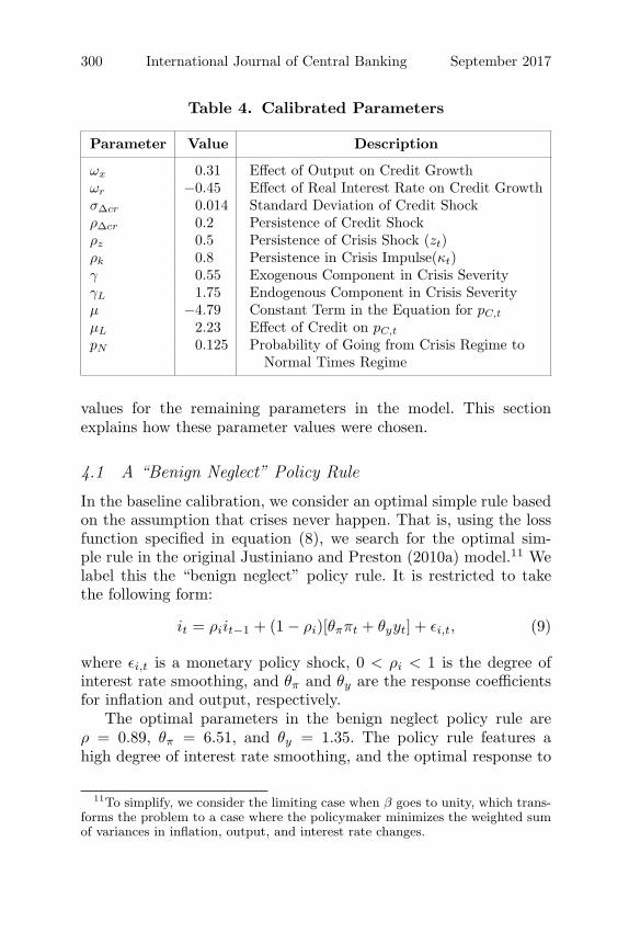
Table 4. Calibrated Parameters

Parameter Value Description

ωx 0.31 Effect of Output on Credit Growthωr −0.45 Effect of Real Interest Rate on Credit GrowthσΔcr 0.014 Standard Deviation of Credit ShockρΔcr 0.2 Persistence of Credit Shockρz 0.5 Persistence of Crisis Shock (zt)ρk 0.8 Persistence in Crisis Impulse(κt)γ 0.55 Exogenous Component in Crisis SeverityγL 1.75 Endogenous Component in Crisis Severityμ −4.79 Constant Term in the Equation for pC,t

μL 2.23 Effect of Credit on pC,t

pN 0.125 Probability of Going from Crisis Regime toNormal Times Regime

values for the remaining parameters in the model. This sectionexplains how these parameter values were chosen.

4.1 A “Benign Neglect” Policy Rule

In the baseline calibration, we consider an optimal simple rule basedon the assumption that crises never happen. That is, using the lossfunction specified in equation (8), we search for the optimal sim-ple rule in the original Justiniano and Preston (2010a) model.11 Welabel this the “benign neglect” policy rule. It is restricted to takethe following form:

it = ρiit−1 + (1 − ρi)[θππt + θyyt] + εi,t, (9)

where εi,t is a monetary policy shock, 0 < ρi < 1 is the degree ofinterest rate smoothing, and θπ and θy are the response coefficientsfor inflation and output, respectively.

The optimal parameters in the benign neglect policy rule areρ = 0.89, θπ = 6.51, and θy = 1.35. The policy rule features ahigh degree of interest rate smoothing, and the optimal response to

11To simplify, we consider the limiting case when β goes to unity, which trans-forms the problem to a case where the policymaker minimizes the weighted sumof variances in inflation, output, and interest rate changes.


inflation is relatively higher than the response to output. This rulewill serve as a benchmark when we later evaluate policy rules thattake the risk of financial crises into account.12

4.2 Credit Dynamics

The quarterly rate of household credit growth is assumed to dependon the output gap and the real interest rate. The effect of outputand the real interest rate on credit are calibrated in two steps. Wefirst calibrate the effect of output on credit by estimating a sim-ple reduced-form equation for household credit growth.13 The pointestimate of the effect of the output gap on credit growth is reportedin table 4. Next, the effect of the real interest rate on credit growthis calibrated to match the response of a monetary policy shock fromthe structural VAR model in Robstad (2014),14 given the calibratedeffect of output on credit. This ensures that real credit declines about0.7–0.8 percent in response to a monetary policy shock that raisesthe nominal interest rate by 1 percentage point at impact.

The credit shock εΔcr,t in equation (3) is assumed to follow anAR(1) process with standard deviation σΔcr and persistence ρΔcr.We calibrate σΔcr and ρΔcr to match (i) the standard deviation inhousehold credit growth and (ii) the correlation between householdcredit growth and output in Norway.15

4.3 The Probability of a Crisis

The probability of a transition from normal times to crisis times(pC,t) is assumed to depend on the five-year real growth in householdcredit (Lt) and is given by (7). We use the estimates documented insection 2.2 to calibrate the parameters μ and μL. The probability

12The benign neglect rule can be thought of as how policymakers saw the worldprior to the global financial crisis from 2007/08.

13We regress household credit growth (C2 households) on the output gap (HP-filtered real GDP for mainland Norway using λ = 3, 000). We estimate the modelwith 2SLS using two lags of the output gap as instruments for the current outputgap.

14Figure 7 in this paper.15The standard deviation of household credit growth and the correlation with

the output gap is empirically (in the model) 1.54 (1.54) and 0.33 (0.38), respec-tively.


of going from a crisis regime to normal times, pN , is assumed to beexogenous and calibrated to give an average duration of crisis of twoyears, requiring pN = 0.125.

4.4 The Severity of a Crisis

In order to calibrate the effect on the output gap in a crisis and howit varies with the pre-crisis credit accumulation, we use the resultsestablished in section 2.3. These results indicate that the unemploy-ment rate on average increases by about 5 percentage points duringa crisis, while a one standard deviation higher credit accumulationbefore the crisis increases the unemployment rate by 0.75 percentagepoints the first two years of the crisis.

We use Okun’s law with a parameter of −2 to map the unem-ployment rate to the output gap. Our results then suggest that theaverage fall in the output gap during a crisis should be approxi-mately 10 percentage points, while one standard deviation highercredit accumulation before the crisis should make output fall byabout 1.5 percentage points more over the first two years of a crisis.With a standard deviation in the five-year growth in real credit of17 percent, this implies that output falls by 1.5/17 = 0.09 percent-age points more on average during a crisis if the five-year growthin real credit is 1 percentage point higher before the crisis, all elseequal. This is in line with the effects of Jorda, Schularick, and Taylor(2013); see the discussion in Svensson (2016, appendix D).

To make the model match the empirical results, we perform localprojections on simulated data from the model. The parameters γ andγL in equation (6) are then selected to match the results from theempirical projections.16 The results are shown in figure 2.

16Since the output dynamics during a crisis in the model may differ fromthe implied dynamics illustrated in figure 1, we match the average differencebetween the output paths over horizon h = 1, . . . , H in order to capture thatthe severity of a crisis is both deeper and more protracted when credit growthis high in the boom preceding a crisis. Formally, we let yh and yL

h be theimplied output paths based on the local projection in figure 1 when creditgrowth at the peak is on average and one standard deviation higher, respec-tively, and we let yh and yL

h be the counterparts based on simulations of themodel. We choose γ and γL to minimize the following loss function: L(γ, γL) =(minh yh −minh yh)2 + 1

H(∑H

h=1 (yLh − yh)−

∑Hh=1 (yL

h − yh))2. We use H = 8 tobe consistent with the assumption of an average duration of crisis of two years.


Figure 2. Output Dynamics during Crises in the Model

1 2 3 4 5 6 7 8−14

−12

−10

−8

−6

−4

−2

0

2

4

Number of quarters from start of crisis

Per

cent

Average depth of crisis+ effect of a 1 std. higher 5−year credit growth before crises

Figure 2 shows that, in the model, the output gap falls by approx-imately 10 percentage points during a crisis if the five-year real creditgrowth prior to the crisis is at its average level. Compared with theempirical results in figure 1, the model generates an output paththat returns relatively quickly to the pre-crisis level. The averagedifference between the two paths illustrated in figure 2 is approxi-mately 1.3 percent, somewhat lower than the calibration target of1.5 percent.

5. Properties of the Calibrated Model

Before we turn to the analysis of policy rules that take the risk of afinancial crisis into account, it is useful to consider some propertiesof the model under the benign neglect policy rule. We ask two ques-tions. First, are there any potential benefits from LAW policies inthis economy? Second, how strong is the impact of monetary policyon key variables?

To help answer the first question, table 5 shows statistics fromsimulations of two versions of the model. First we simulate thebenchmark calibrated version, and then a version where crises neverhappen. The latter simulation can be interpreted as the case wheremacro stabilization policies have managed to remove crisis risk com-pletely with no side effects to the rest of the economy.


Table 5. Simulations under the Benign Neglect Policywith and without the Possibility of Crises

If CrisesBenchmark Never Happen

Std. Annual Inflation 1.66 1.59Std. Output Gap 2.16 1.67Std. Interest Rate (Ann. %) 3.96 3.17Std. Real Exchange Rate 8.43 8.19Std. Credit Growth 1.64 1.58

Loss 100 79.10Frequency of Crisis (Ann. %) 3.23 0.00

Note: Model standard deviations and the frequency of financial crises are computedby generating 1,000 replications of length 1,000 quarters.

In the benchmark case, the average frequency of crises is about3.2 percent. The volatility (measured by the standard deviation) ofthe output gap is reduced by almost one-quarter when crises areremoved. The central bank loss is reduced by one-fifth. This impliesthat crisis risk is an important source of losses for the central bank,and worthy of further analysis. The next section analyzes whetherLAW policies can reap any of the benefits from lower crisis risk.

In order to shed light on the second question, we start by plottingthe impulse response function (IRF) for key variables to a monetarypolicy shock; see figure 3.

A monetary policy tightening makes the output gap decline byalmost 0.4 percent. Inflation also falls, but it increases in laterperiods due to the depreciation of the real exchange rate. The five-year real credit growth declines gradually, and the response is muchmore persistent than for the other variables. The peak impact isat almost –0.8, which was reported as the calibration target insection 4.2.

We also include the IRF for the probability of a crisis. Since thisis a non-linear function of credit, the IRF depends on the initialsituation of the economy when the monetary policy shock hits.17

17Here we have simulated the IRF from 50,000 model-generated initial states.


Figure 3. Impulse Response Functions under a BenignNeglect Policy Rule

10 20 30 40−0.2

0

0.2

0.4

0.6

0.8

1

1.2Nominal interest rate

Per

cent

age

poin

ts

10 20 30 40−0.15

−0.1

−0.05

0

0.05Annual CPI inflation

Per

cent

10 20 30 40−0.4

−0.3

−0.2

−0.1

0Output gap

Per

cent

10 20 30 40−0.8

−0.6

−0.4

−0.2

0Real exchange rate

Per

cent

10 20 30 40−0.8

−0.6

−0.4

−0.2

05−year real credit growth

Per

cent

10 20 30 40−0.1

−0.08

−0.06

−0.04

−0.02

0

Per

cent

age

poin

ts

Annualized probability of crisis

Median95th percentile

Naturally, the shape of the IRF for the crisis probability resemblesthe shape of the IRF for the five-year real credit growth. An increasein the policy rate by 1 percentage point leads to a decline in the prob-ability of a crisis of about 0.05 percentage points. This amounts toa decline in pC from, e.g., 3.2 to 3.15 percent. A larger response canbe expected when credit is initially at a higher level. The lower areaof the 95th percentile gives a decline of more than 0.08 percentagepoints.

It is also relevant to check how monetary policy shocks can affectcrisis outcomes. Figure 4 shows how a positive monetary shock isexpected to affect the output gap if a crisis was to happen sometimein the two-year period after the shock. This also depends on the ini-tial situation of the economy, so it has a distribution across differentinitial states. The median response tells us that a contractionary


Figure 4. The Effect of a Positive Interest Rate Shock onthe Output Gap during a Crisis (percentage points)

0 1 2 3 4 5 6 7−0.4

−0.3

−0.2

−0.1

0

0.1

Per

cent

age

poin

ts

Periods since start of crisis

Median75th percentile95th percentile

Note: Distribution of crisis outcomes from simulations are based on 50,000different initial states.

monetary policy shock, through reducing credit, will increase thelevel of the output gap during crises, i.e., reduce the severity. Thelargest effect comes in the third period of the crisis, where output isincreased by almost 0.1 percentage point. Hence, if the typical fallin output in the third period of the crisis is 10 percentage points,the monetary policy shock lowers it to 9.9 percentage points.

Sometimes the sign shifts, implying that monetary policy makesthe output gap even more negative during crises, explaining whythe 95th percentile covers area below zero. That happens if a crisisoccurs shortly after the monetary policy shock. In such cases theeconomy is initially weaker due to the monetary policy shock, whilethe effect of the shock on credit is still quite small.

In summary, monetary policy has the potential to reduce theexpected cost of crises, both through a reduction in the probabilityof a crisis and the potential severity. There will, however, also bea cost associated with such a policy through increased volatility innormal times, especially when there is a trade-off between stabilizingtraditional target variables and financial stability.


6. Systematic LAW with Simple Interest Rate Rules

We will now use the model extended with credit and crisis risk toevaluate whether it can be beneficial for the central bank to con-duct systematic LAW policies. In particular, we will compare theoutcomes under the benign neglect rule and a LAW specification ofthe following form:

it = ρiit−1 + (1 − ρi)[θππt + θyyt + (1 − Ω)1Δcrt>0θL(Δcrt − πt)]

+ εi,t. (10)

θL is the response coefficient on real credit growth. We assume anasymmetric response to credit, where 1 = 1 if real credit growth ispositive and zero otherwise. Furthermore, we assume that the cen-tral bank does not respond directly to credit growth during crises.The other coefficients have the same interpretation as those in (9).

The motivation for analyzing an asymmetric policy rule is that,in practice, it is natural to think about LAW policies in the contextof high credit growth.18 This means that the interest rate will bekept higher than what is justified by the (medium-term) outlook forinflation and output when credit growth is higher than some thresh-old. To be pragmatic, we set this threshold to zero (i.e., when realcredit growth is above trend).

Table 6 compares the benign neglect policy rule established insection 4 with three different (optimized) policy rules that take therisk of a financial crisis into account.

The first policy rule we consider is labeled LAW. In this case,we optimize with respect to all the coefficients in the Taylor rule(10). Introducing endogenous financial crises changes the optimizedparameters in several ways. First, the response to output rela-tive to inflation increases and the degree of interest rate smooth-ing is reduced. Second, the coefficient on credit growth is positive,meaning that monetary policy should react systematically to creditgrowth.

18For example, Norges Bank (2016) states the following: Conditions that implyan increased risk of particularly adverse economic outcomes should be taken intoaccount when setting the key policy rate. This suggests, among other things,that monetary policy should therefore seek to mitigate the buildup of financialimbalances.


Table 6. Optimal Parameters in SimpleMonetary Policy Rules

BenignParameter Neglect LAW C-LAW I C-LAW II

ρi 0.89 0.88 0.89 0.86θπ 6.51 5.80 6.51 4.60θy 1.35 1.45 1.35 1.24θL — 0.51 0.64 —

Notes: The optimal coefficients are obtained by minimizing the weighted sum ofvariances in (annualized) inflation, output, and the change in the nominal interestrate (annualized). The weight on the output gap and the change in the nominalinterest rate is λy = 2/3 and λi = 1/4, respectively.

The two remaining policy rules we consider are constrained ver-sions of the LAW policy rule. In the first version, we fix the param-eters on the lagged interest rate, inflation, and output in the benignneglect policy rule and reoptimize with respect to credit growth only.We label this policy rule C-LAW I. In the second version, we setthe coefficient on credit growth to zero and reoptimize with respectinflation, output, and the lagged interest rate (C-LAW II ). Theseconstrained versions of the LAW policy are meant to illustrate therelative importance of introducing credit growth as an additionalelement in the Taylor rule and changing the relative response to tra-ditional target variables. While the first constrained version of theLAW policy responds relatively more to credit growth, the secondversion compensates for the inability to respond directly to creditby increasing the relative response to output. It also features a lowerdegree of interest rate smoothing.

Table 7 evaluates the different policy rules with regard to thevariation in some key variables, the total central bank loss, and thefrequency of crises (the unconditional crisis probability). First, com-paring the benign neglect policy rule with the different LAW rules,the latter lead to reduced volatility in output but increased costsin terms of higher inflation volatility. The unconstrained LAW pol-icy reduces the total loss by approximately 3.8 percent, and theunconditional probability of a crisis is reduced by 6 basis points.Comparing the two constrained versions of the LAW policy, the


Table 7. Standard Deviations of Endogenous Variables,Loss, and the Frequency of Crisis under

Different Policy Rules

BenignNeglect LAW C-LAW I C-LAW II

Std. Annual Inflation 1.66 1.74 1.69 1.75Std. Output 2.16 1.83 2.01 1.84Std. Interest Rate (Ann. %) 3.96 3.94 3.90 3.97Std. Real Exchange Rate 8.43 8.44 8.41 8.45Std. Credit Growth 1.64 1.56 1.58 1.58

Loss Relative to Benign Neglect 100.00 96.23 97.62 96.88Frequency of Crises (Ann. %) 3.23 3.17 3.16 3.21

Note: Model standard deviations and the frequency of financial crisis are computed bygenerating 1,000 replications of length 1,000 quarters.

results may suggest that taking financial stability considerationsinto account by changing the relative response to traditional targetvariables generates a relatively large share of the benefits.

Figure 5 shows the distribution of losses under the different pol-icy rules. While the difference in losses between the alternative LAWpolicies is small, it is clear that taking crisis risk into account whensetting the policy rate reduces the magnitude and frequency of tail-risk events.

In order to illustrate the magnitude of the “degree of leaning”under the alternative LAW policies, we simulate the model underthe benign neglect rule, while including the different LAW rules as“cross-checks.” Table 8 shows the difference in the nominal interestrate implied by the respective LAW policies and the actual policyrule (benign neglect) for different states of the economy. Consideringall states of the economy, the LAW policy implies an interest ratethat is approximately 18 basis points higher on average. In periodswith elevated financial stability risks (i.e., when L > 0), the LAWpolicy implies a 26 basis points higher interest rate on average. Theinterest rate is even higher (around 50 basis points) when the realeconomy is strong at the outset (i.e., y > 0). In periods when finan-cial stability risks are elevated but the real economy is weak, theLAW policy implies a somewhat more expansionary policy than the


Figure 5. Distribution of Losses under DifferentPolicy Rules

6 7 8 9 10 11 12 13 14 15 160

0.05

0.1

0.15

0.2

0.25

0.3

0.35

0.4

0.45

Loss (πt2 + λ

y y

t2 + λ

i (Δ i

t)2)

Den

sity

Benign neglectLAWConstrained LAW IConstrained LAW II

Note: The figure shows the distribution of losses under the alternative policyrules.

Table 8. Difference between the Interest Rate underAlternative LAW Policies and the Benign Neglect Policy

Rule for Different States of the Economy(percentage points)

State Frequency* LAW C-LAW I C-LAW II

All States 1.00 0.18 0.20 0.00L > 0 0.49 0.26 0.25 0.05L, y > 0 0.28 0.48 0.35 0.27L > 0, y < 0 0.21 −0.05 0.12 −0.23L < 0 0.51 0.10 0.16 −0.05L, y < 0 0.29 −0.11 0.08 −0.26L < 0, y > 0 0.21 0.38 0.26 0.23

∗The share of time spent in each state.

benign neglect policy. When financial stability risks are relativelylow (L < 0), the LAW policy implies a 10 basis points higher inter-est rate. When both financial stability risks are low and the realeconomy is weak, the interest rate should be 11 basis points lower


in the LAW case. The LAW policy rule calls for a higher interestrate (38 basis points) when the real economy is strong (y > 0), eventhough financial stability risks are low.

6.1 A Persistent Decline in Foreign Interest Rates andFinancial Stability

The persistent decline in foreign interest rates in recent years hascaused a trade-off for many small open economies. In this section weillustrate the dynamics of the economy in normal times and in crisistimes when the central bank reacts to the decline in foreign inter-est rates using the benign neglect rule or the LAW rule. To counterthe effects of lower foreign interest rates on the real exchange rate,inflation, and output, a central bank will respond by reducing thedomestic policy rate. Lower interest rates might in turn fuel thehousing market and increase the accumulation of household credit.This may increase the risk of a financial crisis. In such a scenario, aLAW rule that reduces the interest rate less than what is justifiedonly by the medium-term outlook for inflation and output mightdeliver better outcomes over time.

Figure 6 shows IRFs of a large and persistent negative shock tothe foreign interest rate under the benign neglect rule and the LAWrule. Both policy rules imply a big reduction in the nominal interestrate, but the LAW rule keeps the rate slightly higher. The apprecia-tion of the real exchange rate is greater under the LAW rule and thedrop in the inflation rate is larger. On the other hand, the LAW rulestabilizes output more than the benign neglect rule. Together withthe higher interest rate, this dampens growth in household credit andreduces both the probability and the potential severity of a financialcrisis. Following the negative shock to the foreign interest rate, weimpose a crisis after eight quarters (illustrated by the shaded area infigure 6). The LAW policy reduces the severity of a crisis in terms ofoutput. First, it contributes by restraining credit growth prior to thecrisis. Second, it responds relatively more to the decline in outputand features a lower degree of interest rate smoothing.

The IRFs show what happens when the crisis occurs on a pre-specified date. Figure 7 shows the entire distribution for GDP underthe two policy rules following the negative shock to the foreigninterest rate. The width of the distribution is caused by both (i)


Figure 6. Impulse Responses of a Large and PersistentNegative Shock to Foreign Interest Rates

2 4 6 8 10 12−15

−10

−5

0

5Nominal interest rate

Per

cent

age

poin

ts

2 4 6 8 10 12−4

−2

0

2

4Annual CPI inflation

Per

cent

2 4 6 8 10 12−8

−6

−4

−2

0

2Output gap

Per

cent

2 4 6 8 10 12−10

−5

0

5Real exchange rate

Per

cent

2 4 6 8 10 12−2

0

2

4

65−year real credit growth

Per

cent

2 4 6 8 10 12−0.2

−0.1

0

0.1

0.2

0.3

0.4

0.5

0.6Annualized probability of a crisis

Per

cent

age

poin

ts

Benign neglect LAW Crisis periods

Note: Shaded area indicates a crisis (exogenously imposed after eight quarters).

uncertainty about when the crisis hits and (ii) uncertainty about theseverity of the crisis. By following the LAW policy, one reduces thenegative tail risk in output by dampening the effect of lower inter-national interest rates on the probability and the potential severityof a crisis.

7. Sensitivity

The parameters governing the probability and the effect of creditaccumulation on the severity of a crisis estimated in section 2 arehighly uncertain. In this section, we examine how sensitive theoptimized response to credit growth in the Taylor rule is to thesekey parameters.


Figure 7. Distribution of the Output Gap Following aLarge, Persistent Negative Shock to Foreign Interest

Rate, when Crisis Risk Is the Only Source of Uncertaintyafter the Interest Rate Shock

1 5 9 13 17

−10

−8

−6

−4

−2

0

2

4

−10

−8

−6

−4

−2

0

2

4Benign neglect

Per

cen

t

1 5 9 13 17

−10

−8

−6

−4

−2

0

2

4

−10

−8

−6

−4

−2

0

2

4LAW

Per

cen

t

Note: The dark gray area shows the 95th percentile, while the light grey areashows the 99th percentile of the distribution.

7.1 LAW Policies and the Effect of Crediton the Probability of a Crisis

Figure 8 compares the logit function used in this paper with Ajelloet al. (2015) and estimates of the effect of mortgage credit on theprobability of a crisis for different sample periods reported in Jorda,Schularick, and Taylor (2016).19 While the steady-state probabil-ity used in this paper and the one in Ajello et al. (2015) are sim-ilar, the effect of credit on the probability of a crisis is higher in

19When plotting the probability functions reported in Jorda, Schularick, andTaylor (2016) (table 4, column 2) we have set the constant term equal to theone used in Ajello et al. (2015). The regressions in Jorda, Schularick, and Taylor(2016) are based on the five-year moving average growth rate in mortgage credit,and not the cumulative growth. This has also been corrected for when plottingthe probability functions.


Figure 8. Relationship between Five-Year Real CreditGrowth (L) and the Probability of a Crisis Start

0 5 10 15 20 25 30 35 40 45 500.8

1

1.2

1.4

1.6

1.8

2

2.2

2.4

2.6

Lt

Qua

rter

ly p

roba

bilit

y of

cris

is s

tart

(%

)This paperAjello et al. (2015)Jorda et al (2016) − Full sampleJorda et al. (2016) − Pre−WW2Jorda et al. (2016) − Post−WW2

our paper. However, Jorda, Schularick, and Taylor (2016) documentthat the effect of mortgage credit on the probability of a crisis hasincreased substantially over time. Estimates used in other papersanalyzing LAW policies have typically been based on the long-runhistorical data in Schularick and Taylor (2012) (e.g., Ajello et al.2015 and Svensson 2016), which starts in 1870, while we use datafrom the 1970s. As seen in figure 8, the effect of mortgage crediton the probability used in our paper is close to the effect estimatedon the post–World War II sample in Jorda, Schularick, and Taylor(2016).

To illustrate how sensitive the optimized response to creditgrowth in the Taylor rule is to the underlying assumption aboutthe probability of crisis, table 9 shows optimized parameters for dif-ferent specifications of the crisis probability. We use the specificationreported in Ajello et al. (2015) which features a lower effect of crediton the probability of a crisis. We also examine two cases when theprobability of crisis is exogenous: one where the steady-state proba-bility is relatively high (approximately 3.2 percent annually20) andone where the probability is relatively low (1 percent).

20We have used the steady-state probability reported in Ajello et al. (2015) tofacilitate comparison.


Table 9. Optimal Simple Rules for DifferentCrisis Probabilities

Ajello et al. Exogenous ExogenousLAW (2015) (3.2% Ann.) (1% Ann.)

ρi 0.88 0.87 0.88 0.91θπ 5.80 5.17 5.31 6.48θy 1.45 1.30 1.30 1.46θL 0.51 0.28 0.21 −0.03

Loss* 96.23 96.92 98.13 99.77

∗Relative to the loss simulated under the benign neglect policy rule (using the sameparameters in the logit function for the probability of a crisis).

It is clear that the optimal response to credit growth (and thepotential benefit of LAW) depends on the assumed process for theprobability of a crisis. First, it depends on the crisis probability level.The coefficient on credit growth is low when the crisis probability islow, both in the case of an endogenous and exogenous crisis probabil-ity. In the case of a 1 percent annual exogenous probability of a crisis,the coefficient on credit growth is slightly negative. However, even inthis case the relative coefficient on output is somewhat higher thanin the benign neglect rule. Second, the steepness of the logit func-tion matters. In Ajello et al. (2015), the crisis probability increasesless with accumulated credit growth than in our paper. This isreflected in the coefficient on credit being higher in our benchmarkcalibration (LAW rule) than that implied by Ajello et al. (2015);see table 9.

While the logit function in our benchmark calibration and thealternative functions shown in this section are linear, or close tolinear, introducing more non-linearities may increase the benefitsof leaning against the wind to the extent that monetary policy caninfluence these imbalances. For example, Anundsen et al. (2016) doc-ument that the effect of household credit on the likelihood of a crisisincreases substantially when it coincides with extreme imbalances(or bubble-like behavior) in the housing market. While such non-linearities (or threshold effects) might be very important, they aredifficult to incorporate in the model in a simple way.


Figure 9. The Relationship between the Marginal Effecton GDP during Crisis of a One Standard Deviation Higher

Five-Year Growth in Household Real Credit and theOptimal Response to Credit Growth in the Taylor Rule

−3 −2.5 −2 −1.5 −1 −0.5 0−0.4

−0.2

0

0.2

0.4

0.6

0.8

1

Res

pons

e to

cre

dit g

row

th in

the

Tay

lor

rule

(θL)

Effect of higher debt accumulation on GDP during crisis (percent)

Note: The optimal policy rules are found by searching over an interval of themarginal effect of credit on GDP during a crisis (in steps of –0.25 percent).

7.2 LAW Policies and the Effect of Crediton the Severity of Crisis

The effect of credit accumulation on the decline in GDP duringa crisis was calibrated to match the empirical results established insection 2.3. More precisely, our calibration implies that GDP declinesby approximately 1.5 percentage points more on average during acrisis if the five-year growth in real household credit before the crisisis one standard deviation higher. In order to illustrate the sensitivityof our results regarding this calibration, figure 9 plots the relation-ship between the effect of a one standard deviation higher cumulativereal credit growth on GDP during crisis (horizontal axis) and theoptimal response to credit growth in the Taylor rule.21 The optimalresponse to credit is an increasing function of the effect of crediton GDP during a crisis. If we assume that the severity of a crisis is

21The other coefficients in the Taylor rule are also reoptimized in this exercise.


exogenous (this implies that the effect of pre-crisis credit growth onGDP during a crisis equals zero), the optimal coefficient on creditgrowth is negative instead of positive, implying that monetary pol-icy should, if anything, lean with the wind. Thus, in a case where theseverity of a crisis is exogenous or the effect of credit on GDP duringa crisis is sufficiently small, we find no role for monetary policy torespond countercyclically to credit growth.

8. Conclusion

Whether to use monetary policy to curb high growth in credit andasset prices to contain the risk of financial instability, i.e., to “leanagainst the wind” (LAW), has been the subject of a contentiousdebate. In this paper we have investigated to what extent monetarypolicy should actively aim at mitigating the buildup of financialimbalances. LAW is motivated by agents underestimating financialstability risks. We introduce regime switching into an otherwise stan-dard open-economy New Keynesian model to highlight some impor-tant policy trade-offs. Credit affects the probability of switching to acrisis and the severity of a crisis, but does not affect economic activ-ity in normal times. Credit is in this sense frictionless in normaltimes. A transition from a normal regime to a crisis regime involvesan abrupt reduction in aggregate demand.

We find that the benefits of LAW in terms of a lower frequencyof severe financial recessions exceed costs in terms of higher volatil-ity in normal times when the severity of crisis is endogenous (i.e.,“when credit bites back”). The LAW policy can be implemented byresponding relatively more to fluctuations in output and by respond-ing directly to household credit growth. Compared with a benignneglect policy, the LAW policy rules contribute to a lower loss andreduced tail risk in the economy. The costs are paid in terms ofsomewhat higher inflation volatility and interest rate volatility. Ourqualitative results are robust to alternative specifications for theprobability of a crisis. We also show that the optimal interest rateresponse to credit growth is higher when the severity of a crisis issensitive to changes in accumulated credit growth. When the sever-ity of a crisis is exogenous, then it is, if anything, optimal to leanwith the wind. This nests the results found in the literature, e.g.,Ajello et al. (2015), Alpanda and Ueberfeldt (2016), Pescatori and


Laseen (2016), and Svensson (2016), who find no (or very small) netbenefits of LAW policies, and typically assume either no or a verysmall effect from credit to crisis severity. This difference underlinesthe importance of the assumptions concerning the process whichdetermines the severity of a crisis.

References

Ajello, A., T. Laubach, D. Lopez-Salido, and T. Nakate. 2015.“Financial Stability and Optimal Interest-Rate Policy.” WorkingPaper, Federal Reserve Board (February).

Alpanda, S., and A. Ueberfeldt. 2016. “Should Monetary Policy LeanAgainst Housing Market Booms?” Working Paper No. 2016/19,Bank of Canada.

Anundsen, A. K., K. Gerdrup, F. Hansen, and K. Kragh-Sørensen.2016. “Bubbles and Crises: The Role of House Prices and Credit.”Journal of Applied Econometrics 31 (7): 1291–1311.

Assenmacher-Wesche, K., and S. Gerlach. 2008. “Monetary Pol-icy, Asset Prices and Macroeconomic Conditions: A Panel-VARStudy.” Working Paper No. 149, National Bank of Belgium.

Bianchi, J. 2011. “Overborrowing and Systemic Externalities in theBusiness Cycle.” American Economic Review 101 (7): 3400–3426.

Bianchi, J., and E. G. Mendoza. 2013. “Optimal Time-ConsistentMacroprudential Policy.” NBER Working Paper No. 19704.

Bussiere, M., and M. Fratzscher. 2006. “Towards a New Early Warn-ing System of Financial Crises.” Journal of International Moneyand Finance 25 (6): 953–73.

Curdia, V., and M. Woodford. 2009. “Credit Frictions and OptimalMonetary Policy.” BIS Working Paper No. 278.

———. 2010. “Credit Spreads and Monetary Policy.” Journal ofMoney, Credit and Banking 42 (s1): 3–35.

Dynan, K. 2012. “Is a Household Debt Overhang Holding BackConsumption?” Brookings Papers on Economic Activity 44 (1,Spring): 299–362.

Galı, J., and T. Monacelli. 2005. “Monetary Policy and ExchangeRate Volatility in a Small Open Economy.” Review of EconomicStudies 72 (3): 707–34.


Gelain, P., K. J. Lansing, and G. J. Natvik. 2015. “Leaning Againstthe Credit Cycle.” Working Paper No. 4/2015, Norges Bank(February).

Gerdrup, K., F. Hansen, T. Krogh, and J. Maih. 2016. “LeaningAgainst the Wind When Credit Bites Back.” Working Paper No.9/2016, Norges Bank.

Goodhart, C., and B. Hofmann. 2008. “House Prices, Money, Credit,and the Macroeconomy.” Oxford Review of Economic Policy 24(1): 180–205.

Hansen, F., and K. N. Torstensen. 2016. “Does High Debt Growthin Upturns Lead to a More Pronounced Fall in Consumption inDownturns?” Economic Commentaries No. 8/2016, Norges Bank.

Jorda, O. 2005. “Estimation and Inference of Impulse Responses byLocal Projections.” American Economic Review 95 (1): 161–82.

Jorda, O., M. Schularick, and A. M. Taylor. 2013. “When CreditBites Back.” Journal of Money, Credit and Banking 45 (s2):3–28.

———. 2016. “The Great Mortgaging: Housing Finance, Crises andBusiness Cycles.” Economic Policy 31 (85): 107–52.

Justiniano, A., and B. Preston. 2010a. “Can Structural Small Open-Economy Models Account for the Influence of Foreign Distur-bances?” Journal of International Economics 81 (1): 61–74.

———. 2010b. “Monetary Policy and Uncertainty in an EmpiricalSmall Open-Economy Model.” Journal of Applied Econometrics25 (1): 93–128.

Laseen, S., and I. Strid. 2013. “Debt Dynamics and Monetary Policy:A Note.” Working Paper No. 283, Sveriges Riksbank.

Lorenzoni, G. 2008. “Inefficient Credit Booms.” Review of EconomicStudies 75 (3): 809–33.

Mian, A., and A. Sufi. 2011. “House Prices, Home Equity-BasedBorrowing, and the US Household Leverage Crisis.” AmericanEconomic Review 101 (5): 2132–56.

Monacelli, T. 2005. “Monetary Policy in a Low Pass-Through Envi-ronment.” Journal of Money, Credit and Banking 37 (6): 1047–66.

Musso, A., S. Neri, and L. Stracca. 2011. “Housing, Consumptionand Monetary Policy: How Different Are the US and the EuroArea?” Journal of Banking and Finance 35 (11): 3019–41.


Norges Bank. 2012. “Monetary Policy Report 3/12.” TechnicalReport No. 3.

———. 2016. “Monetary Policy Report with Financial StabilityAssessment 3/16.” Technical Report No. 3.

Pescatori, A., and S. Laseen. 2016. “Financial Stability and Interest-Rate Policy: A Quantitative Assessment of Costs and Benefits.”IMF Working Paper No. 16/73 (March).

Reinhart, C. M., and K. S. Rogoff. 2008. “Is the 2007 US Sub-prime Financial Crisis So Different? An International HistoricalComparison.” American Economic Review 98 (2): 339–44.

Robstad, Ø. 2014. “House Prices, Credit and the Effect of Mone-tary Policy in Norway: Evidence from Structural VAR Models.”Working Paper No. 5/2014, Norges Bank.

Schularick, M., and A. M. Taylor. 2012. “Credit Booms Gone Bust:Monetary Policy, Leverage Cycles, and Financial Crises, 1870–2008.” American Economic Review 102 (2): 1029–61.

Smets, F. 2014. “Financial Stability and Monetary Policy: HowClosely Interlinked?” International Journal of Central Banking10 (2): 263–300.

Svensson, L. E. O. 2014. “Inflation Targeting and ‘Leaning Againstthe Wind’.” International Journal of Central Banking 10 (2):103–14.

———. 2016. “Cost-benefit Analysis of Leaning Against the Wind:Are Costs Larger Also with Less Effective Macroprudential Pol-icy?” NBER Working Paper No. 21902 (January).

Taylor, A. M. 2015. “Credit, Financial Stability, and the Macroecon-omy.” NBER Working Paper No. 21039 (March).

Woodford, M. 2012. “Inflation Targeting and Financial Stability.”NBER Working Paper No. 17967 (April).

leaning against the wind when credit bites back - ijcb · leaning against the wind when credit...

Documents